A new partition identity coming from complex dynamics

Abstract

We present a new identity involving compositions (i.e. ordered partitions of natural numbers). The Formula has its origin in complex dynamical systems and appears when counting, in the polynomial family $\{f_{c}:z\mapsto z^{d}+c\}$, periodic critical orbits with equivalent itineraries. We give two different proofs of the identity; one following the original approach in dynamics and another with purely combinatorial methods.

1 Introduction

The field of dynamical systems takes frequent advantage of combinatorial techniques to classify all sorts of dynamic phenomena. Often the tools borrowed are classic, so there are few opportunities for feedback. In this note, we introduce a previously unknown identity in the theory of partitions, which arose from dynamical considerations. We will give two different proofs of the formula; one that illustrates the original approach in dynamics and a second one using the more traditional methods of enumerative combinatorics.

Definitions:  Let $n\in\mathbb{N}$. A composition of $n$ in $r$ parts is a partition $P:=[a_{1}+\ldots+a_{r}=n]$ that takes into account the order of the parts $a_{j}.$ An H-composition is a composition satisfying $a_{1}\geq a_{j}$ for all $j\leq r$. We use $\mathcal{H}(n)$ to denote the collection of H-compositions of $n.$

The multiplicity $\omega$ of $P\in\mathcal{H}(n)$ is defined as the number of parts other than $a_{1}$, equal to $a_{1};$ that is, $\omega(P)=\#\{j>1\mid a_{j}=a_{1}\}$.

Theorem 1.1

For all $n,d\in\mathbb{N}$ the following identity holds

$$\sum_{P\in\mathcal{H}(n)}\varphi(a_{1})\cdot(d-1)^{r-\omega(P)}\cdot d^{\omega(P)}=d^{n}-1$$ (1.1)

where $\varphi$ represents Euler’s totient function.

Example:  $\mathcal{H}(5)=\{5,4+1,3+2,3+1+1,2+2+1,2+1+2,2+1+1+1,1+1+1+1+1\}$. For degree $d=3$, the formula yields:

$$(4\cdot 2\cdot 1)+(2\cdot 2^{2}\cdot 1)+(2\cdot 2^{2}\cdot 1)+(2\cdot 2^{3}\cdot 1)+(1\cdot 2^{2}\cdot 3)+$$

$$+(1\cdot 2^{2}\cdot 3)+(1\cdot 2^{4}\cdot 1)+(1\cdot 2\cdot 3^{4})=242=3^{5}-1$$

Formula 1.1 was first detected in an effort to list the possible combinatorial behaviors of critically periodic orbits in the family of complex polynomials $\{f_{c}:z\mapsto z^{d}+c\mid c\in\mathbb{C}\}$ of fixed degree $d$. Every polynomial function $f:\mathbb{C}\longrightarrow\mathbb{C}$ has associated a compact set $K$, its filled Julia set, that is invariant under $f$. When the critical point is periodic, $f$ is described by a finite amount of data that encodes the location in $K$ of points in the orbit of 0. Theorem 1.1 is proved by counting polynomials with equivalent descriptions.

In Section 2 we provide a condensed review of the relevant concepts from complex dynamics. This will furnish a language to describe the dynamical picture and give some intuition on the behavior of critical orbits. Admittedly, the statements that we need to quote far exceed our limitations of space, and the consequence is a constant referral to the literature. We would like to call attention to [E] and [P]. These works deserve more publicity as they clarify the status of many folk results that had no prior reference.

Section 3 uses the material introduced before to prove Theorem 1.1 from the viewpoint of complex dynamics. Even though the proof of several supporting claims is deferred to the references, the inclusion of this method is justified by its potential to uncover similar identities. This is briefly mentioned at the end of the Section, where a few remarks are made on the combinatorial structure of Formula (1.1).

A self-contained proof of the Formula, relying exclusively on enumerative combinatorics, is presented in Section 4.

2 Basics in Complex Dynamics

In this section we sketch the basic material in dynamics of polynomials in one complex variable. Proofs of the results stated and further information can be found in [DH1], [M1] and [E]. The focus here will be on binomials of the form $f_{c}(z)=z^{d}+c.$ This family covers all affine conjugacy classes of polynomials with exactly one critical point. For any point $z$, the sequence $\big{\{}z,f_{c}(z),f_{c}^{2}(z),\ldots\big{\}}$ of $z$ is called the orbit of $f_{c}$ and is denoted $\mathcal{O}(z)$.

The filled Julia set associated to $f_{c}$ is

$$K_{c}=\big{\{}z\in\mathbb{C}\mid\mathcal{O}(z)\text{ is bounded}\big{\}}.$$ (2.2)

$K_{c}$ is a perfect set; i.e. it contains all its accumulation points. It is totally invariant under $f_{c}$; that is, $f_{c}(K_{c})=f_{c}^{-1}(K_{c})=K_{c}.$ Depending on whether the critical point belongs to the filled Julia set or not, $K_{c}$ is simply connected or a Cantor set. Moreover, since $f_{c}$ is a $d$ to 1 cover of $\mathbb{C}$ branched only at the critical point, $K_{c}$ has $d$-fold rotational symmetry around 0.

A point $z$ is called periodic if $f_{c}^{n}(z)=z$ for some $n\geq 1$. The least such $n$ is called the period of $z$ and the value $\lambda=\left(f_{c}^{n}\right)^{\prime}(z)$ associated to $\mathcal{O}(z)$ is the multiplier of the orbit. When $n=1,$ $z$ is a fixed point. A periodic orbit is called attracting, indifferent or repelling depending on whether $|\lambda|$ is less than, equal or greater than 1. Note that when the critical point belongs to a periodic orbit, the multiplier is 0; we speak then of an superattracting orbit or say that the map $f_{c}$ has periodic critical orbit.

With the exception of $z^{2}-\frac{3}{4},$ every binomial $z^{d}+c$ has at least one periodic orbit of every period. In particular, by the Fundamental Theorem of Algebra, $f_{c}$ always has $d$ fixed points counted with multiplicity.

Most elementary dynamical properties can be deduced from the behavior of critical points and their relation to periodic orbits. The pioneering work of P. Fatou and G. Julia around 1918 produced the following results (valid for arbitrary complex polynomials; see [DH1] or [M1]):

1. To every attracting orbit $\mathcal{O}(z)$ corresponds at least one critical point $c_{0}$ such that $\mathcal{O}(c_{0})$ is captured in a neighborhood of $\mathcal{O}(z)$ and eventually converges to this orbit.

2. Attracting orbits are contained in the interior of the filled Julia set $K,$ whereas repelling orbits belong to $\partial K.$ Moreover, $\partial K$ is the closure of the union of all repelling orbits.

In the case that we study, the only critical point of $f_{c}(z)=z^{d}+c$ is 0, so statement J1 implies that $f_{c}$ can have at most one attracting orbit $\mathcal{O}_{\text{attr}}$. If this orbit exists, the iterates of 0 converge to $\mathcal{O}_{\text{attr}}$; then, $\mathcal{O}(0)$ is bounded and it follows from (2.2) that $K_{c}$ is simply connected.

In the remainder of this Section $c$ is chosen so that $\mathcal{O}_{\text{attr}}$ exists and has period at least 2. Then all fixed points will be repelling and in particular, belong to $\partial K_{c}$. To understand better the geometry of $K_{c}$ consider the left picture in Figure 1. Of the $d$ fixed points, exactly one, denoted $\alpha,$ has the property that $K_{c}\setminus\alpha$ splits into several disjoint components. The component that contains 0 will contain also the remaining $d-1$ fixed points.

Notice that $K_{c}$ has a ”fractal structure”. This is illustrated for instance by the fact that all $n$-fold preimages of $\alpha$ separate $K_{c}$ into as many components as $\alpha$ does. Moreover, such preimages are dense in $\partial K_{c}$.

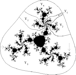
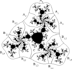
Figure 1: Let $c=(.387848...)+i(.6853...).$ The left picture shows the filled Julia set $K_{c}$ of the cubic map $z^{3}+c,$ covered by level 0 of the puzzle. The center of symmetry is at 0, the point where the rays converge is $\alpha$ and the other fixed points are marked by dotted arrows. In this example the rotation number around $\alpha$ is $\rho_{\alpha}=\frac{2}{5}$ and the ray angles are $\frac{5}{121}\mapsto\frac{15}{121}\mapsto\frac{45}{121}\mapsto\frac{14}{121}\mapsto\frac{42}{121}\mapsto\frac{5}{121}$. The right picture illustrates level 1 of the puzzle for the same map.

Let $\phi_{c}:\widehat{\mathbb{C}}\setminus K_{c}\longrightarrow\widehat{\mathbb{C}}\setminus\mathbb{D}$ be the Riemann map between the complements of $K_{c}$ and the unit disk, normalized to have derivative 1 at $\infty.$ The pull-back by $\phi_{c}$ of concentric circles ($|\zeta|=r,$ with $\zeta\in\mathbb{C}$) yields a family of equipotential curves enclosing $K_{c}.$ Similarly, the pull-back of radial lines ($\arg\zeta=\theta$) results in a family of exterior rays emanating from $K_{c}.$ These two families of curves form mutually orthogonal foliations of $\mathbb{C}\setminus K_{c}.$ The equipotential curve of radius $r>1$ and the external ray of angle $\theta$ will be denoted by $e_{r}$ and $r_{\theta}$ respectively.

The appeal of working with foliations by equipotentials and external rays lies in the fact that they are invariant under the action of $f_{c};$ more precisely, we have the relations

$$f_{c}(e_{r})=e_{(r^{d})}\hskip 21.68121ptf_{c}(r_{\theta})=r_{(d\theta)}$$ (2.3)

It is important to point out that the normalization of $\phi_{c}$ determines the branch of $f_{c}^{-1}(r_{(d\theta)})$ that corresponds to $r_{\theta}$. Property (2.3) of the equipotential and ray foliations is the basis for the definition of the Yoccoz puzzle: Fix the neighborhood $U$ of $K_{c}$ bounded by the equipotential of radius 2 (any other radius $>1$ will do) and consider the collection $\mathcal{R}_{\alpha}$ of rays landing at $\alpha$; refer to Figure 1.

$\mathcal{R}_{\alpha}$ is a finite set and it is known that $f_{c}$ acts on it by a cyclic permutation. If each ray is sent counterclockwise to the ray $p$ positions ahead, the rotation number around $\alpha$ is given by $\rho_{\alpha}=\frac{p}{q}$ where $q=|\mathcal{R}_{\alpha}|,$ $p<q$ and $\text{gcd}(p,q)=1.$ The rays in $\mathcal{R}_{\alpha}$ have rational angles that depend on the values $\rho_{\alpha}$ and $d$; they split the region $U$ into $q$ connected components whose closures will be called the puzzle pieces of level $0$ and denoted $Y_{0},Y_{1},\ldots,Y_{q-1}.$ Here the subindices are residues modulo $q$ and are chosen so that $0\in Y_{0}$ and $f_{c}\left(K_{c}\cap Y_{j}\right)=K_{c}\cap Y_{j+1}$ for $j=1,\ldots,q-1$; in particular, the critical value $c$ is in $Y_{1}$. The combinatorial richness hidden in this picture follows from the fact that

$$f_{c}\left(K_{c}\cap Y_{0}\right)=K_{c},$$ (2.4)

creating multiple overlappings; we expand on this situation below, where level 1 of the puzzle is discussed in more detail.

The puzzle pieces of level $m$ are defined as the closures of the connected components of $f_{c}^{-m}\big{(}\bigcup\text{ int\,}Y_{j}\big{)}$ for $j=0\ldots q-1.$ The resulting family $\mathcal{Y}_{c}$ of puzzle pieces of all levels has the following properties:

1. Each piece is a closed topological disk whose boundary is formed by segments of rays landing at preimages of $\alpha$ and segments of an equipotential curve. To each level of the puzzle there corresponds one equipotential.

2. There are $(q-1)d^{m}+1$ pieces of level $m$ and they form a covering of $K_{c}.$ The unique piece that contains the critical point is called the critical piece of level $m$.

3. Any two puzzle pieces either are nested (with the piece of higher level contained in the piece of lower level), or have disjoint interiors.

4. The image of any piece $Y$ of level $m\geq 1$ is a piece $Y^{\prime}$ of level $m-1$. The restricted map $f_{c}:\text{int\,}Y\longrightarrow\text{int}Y^{\prime}$ is a $d$ to 1 branched covering or a conformal homeomorphism, depending on whether $Y$ is critical or not.

Next, we will give names to the pieces of level 1 and describe briefly their adjacencies and behavior under $f_{c}$; consult the right side of Figure 1 for reference and [E], [S] for information on the case $d>2$. Let $C$ be the critical piece of level 1. $C$ has $d$-fold symmetry and the intersection of its boundary with $K_{c}$ consists of all the points in $f_{c}^{-1}(\alpha)$, including $\alpha$ itself (see Property Y1). We label these points $\alpha,\alpha_{1},\alpha_{2},\ldots,\alpha_{d-1}$ as they are located clockwise on $\partial C.$

Besides $C$, there is a fan of pieces around $\alpha$; we call them $A_{1},\ldots,A_{q-1}$. Here, labels are chosen so that $K_{c}\cap A_{j}=K_{c}\cap Y_{j}$. Thus, $f_{c}(A_{j})=Y_{j+1}$ ($j=1,\ldots,q-1$) is 1 to 1, while $f(C)=Y_{1}$ is a $d$ to 1 branched cover; compare Property Y4.

The picture is similar around all $\alpha_{k}$. There are $q$ pieces $C,\,B_{k,1},\,\ldots,\,B_{k,q-1}$, but here $f_{c}$ does not permute the pieces around $\alpha_{k}$; instead $f_{c}(B_{k,j})=Y_{j+1}$. In short, each $Y_{j}\,(j\neq 1)$ has $d$ preimages $A_{j-1},B_{1,j-1},\ldots,B_{d-1,j-1}$, while $f_{c}^{-1}(Y_{1})=C$. Here again the indices are residues modulo $q$ so $f_{c}(B_{k,q-1})=Y_{0}$ for any $1\leq q\leq d-1$.

As a consequence, consider a point $z\in A_{j}\cap K_{c}$. Its orbit is forced to cyclically follow the rest of the fan $A_{j+1},A_{j+2},\ldots$ around $\alpha$ until $f^{q-j-1}(z)\in A_{q-1}\cap K_{c}$ and, one step later, $f^{q-j}(z)\in Y_{0}\cap K_{c}$. Because of (2.4), the next iterate could be located anywhere in $K_{c}$ depending on the exact position of $f^{q-j}(z)$ within $Y_{0}$.

3 Counting Hyperbolic Components

When the critical orbit $\mathcal{O}(0)$ of $f_{c}$ is periodic, its behavior can be classified according to the disposition within $K_{c}$ of the points in $\mathcal{O}(0)$.

The first proof of Formula (1.1) will be based on a careful study of the different patterns attainable by the critical orbits of critically periodic binomials.

Definition:  A $d$-center is a parameter $c$ such that the map $f_{c}(z)=z^{d}+c$ has periodic critical orbit. We will refer to any $n$ for which $f_{c}^{n}(0)=0$ as a period of the $d$-center.

Lemma 3.1

The number of different $d$-centers with period $n$ is $d^{n-1}$.

Proof (Gleason [DH1, exposé XIX]):  Given $n$ we want to count all the solutions $c$ of the equation $f_{c}^{n}(0)=0$. Since $f_{c}(0)=c$, this is equivalent to count the solutions of $f_{c}^{n-1}(c)=0$. This is a polynomial of degree $d^{n-1}$ in $c$; hence we only need to show that all its solutions are different.

Define the family of polynomials $\big{\{}h_{r}\in\mathbb{Z}[z]\big{\}}$ by the recursion $h_{0}(z)=z$, $h_{r}(z)=\big{(}h_{r-1}(z)\big{)}^{d}+z$, so that the critical orbit of $f_{c}$ returns to 0 after $n$ iterations if and only ifthat our condition reads $h_{n-1}(c)=0$. Each $h_{r}(z)$ is a monic polynomial with integer coefficients, showing that $c$ belongs to the ring $\mathbb{A}$ of algebraic integers.

Suppose $c$ is a multiple root of $h_{n}(z)$; that is, $h_{n}^{\prime}(c)=0$. From $h_{n}^{\prime}(z)=d\big{(}h_{n-1}(z)\big{)}^{d-1}\cdot h_{n-1}^{\prime}(z)+1$ we conclude that $\big{(}h_{n-1}(c)\big{)}^{d-1}\cdot h_{n-1}^{\prime}(c)=\frac{-1}{d}$. By the additive/multiplicative closure of $\mathbb{A}$, the left hand expression is again an algebraic integer; thus $\frac{-1}{d}\in\mathbb{Q}\cap\mathbb{A}=\mathbb{Z}$ ! (refer for instance to [D]). This contradiction shows that $c$ must be a simple root of $h_{n}(z)$ and the result follows. $\square$

Definitions:  Choose a $d$-center $c$ with period $n$ and let $\text{Crit}_{0}$ be the ordered set $\big{\{}z_{0},z_{1},\ldots,z_{n}\big{\}}$ where $z_{j}=f_{c}^{j}(0),\,j=1,\ldots,n$ describes one period of the critical orbit $\mathcal{O}(0)$. Let $Z_{j}$ be the puzzle piece of level $n-j$ that contains $z_{j}$; in particular, $Z_{n}$ is the critical piece $Y_{0}$. It is convenient to think of the family $Z_{n},\ldots,Z_{0}$ as defined in descending order of indices by the finite recursion $Z_{n}=Y_{0},\,f_{c}(Z_{j-1})=Z_{j}\,(j=n,\ldots,1)$. Accordingly we will say that $(Z_{j-1},z_{j-1})$ is the pull-back of $(Z_{j},z_{j})$ along $\text{Crit}_{0}$. By Property Y4, either $Z_{j}$ contains the critical value $c$ and $Z_{j-1}=f_{c}^{-1}(Z_{j})$ or $Z_{j-1}$ is one of the $d$ pieces that constitute $f_{c}^{-1}(Z_{j})$.

We will associate to $c$ an itinerary $\big{(}(a_{1},b_{1}),\ldots,(a_{r},b_{r})\big{)}$ as follows. Consider the subsequence $\zeta_{0},\ldots,\zeta_{r}$ of those points in $\text{Crit}_{0}$ that lie in $Y_{0}$. In particular $\zeta_{0}=0$, $\zeta_{1}=z_{q}$ and $\zeta_{r}=0$ again. The numbers $a_{i}$ are defined by the relation $f_{c}^{a_{i}}(\zeta_{i-1})=\zeta_{i}$. Observe that $a_{i}=q$ exactly when $\zeta_{i-1}\in C$ (this includes the case $\zeta_{0}=0\,\,\Rightarrow\,\,a_{1}=q$). When $a_{i}=q$ we let $b_{i}=0$. Otherwise $a_{i}<q$, and then $\zeta_{i-1}\in B_{k,q-a_{i}}$ for some $k$. The term $q-a_{i}$ appears simply because $f_{c}(\zeta_{i-1})\in f_{c}(B_{k,q-a_{i}})=A_{q-a_{i}+1}$ as required by the definition of $a_{i}$ (compare with the discussion at the end of Section 2). In this situation we let $b_{i}=k$. Every pair $(a_{i},b_{i})$ will be called a leg of the itinerary.

From the definition of the $a_{i}$ it is immediate that $f_{c}^{n}(0)=f_{c}^{a_{r}}\circ\ldots\circ f_{c}^{a_{1}}(0)$ and therefore $a_{1}+\ldots+a_{r}=n$. Since $a_{1}=q\geq a_{j}$ ($1<j\leq r$), it follows that $a_{1}+\ldots+a_{r}=n$ is an H-composition of $n$ with $r$ parts and we denote it by $P(c)$.

The above definitions afford us the means to describe critical orbits. The distribution of elements of $\text{Crit}_{0}$ within $K_{c}$ is well conveyed by its itinerary, even though theses objects are not in 1 to 1 correspondence. The core result in this Section makes precise just how much extra information is required to single out a particular $d$-center:

Proposition 3.2

Let $P$ denote an H-composition $a_{1}+\ldots+a_{r}=n$ with $a_{1}>1$ and multiplicity $\omega(P)=w$. Then the total number of $d$-centers $c$ having $n$ as a period and such that $P(c)=P$ is

$$\#\big{\{}c\text{ \rm is a $d$-center }\mid P(c)=P\big{\}}=\varphi(a_{1})\cdot(d-1)^{r-w}\cdot d^{w}.$$ (3.5)

Theorem 1.1 follows from the previous results. Lemma 3.1 determines the total number of $d$-centers with period $n$, while Proposition 3.2 sorts them by combinatorial type.

Proof of Theorem 1.1:  Note that the binomial $f_{0}(z)=z^{d}$ is the only one with 0 as a fixed point. Thus, the H-composition $1+1+\ldots+1=n$ can be associated to the single $d$-center $c=0$, regardless of the value of $n$. The other $d$-centers are classified in Proposition 3.2 according to their associated H-composition, so by Lemma 3.1 the total of $d$-centers is

$$\text{\Large 1}\hskip 14.45377pt+\sum_{\begin{subarray}{c}P\in\mathcal{H}(n)\\ a_{1}>1\end{subarray}}\varphi(a_{1})(d-1)^{r-\omega(P)}p^{\omega(P)}=d^{n-1}.$$

Since $\omega(1+1+\ldots+1)=n-1$, the LHS can be modified to incorporate this particular case under the sum symbol to coincide with the sum in Formula (1.1). The adjusted value on the RHS becomes $d^{n-1}-1+(d-1)d^{n-1}=d^{n}-1$ as claimed. $\square$

Proof of Proposition 3.2:  The proof will be divided in 2 parts according to the structure of the given H-composition $P$. Essentially we have to handle apart the possibility that $P$ admits $d$-centers with period smaller than $n$. Let us describe first the situation of period less than $n$ in order to present an outline of the proof.

Suppose that for some $z^{d}+c$ and $j\leq n-1$, the piece $Z_{n-j}$ contains 0 as well as $z_{n-j}\in\text{Crit}_{0}$. Since $z_{n}=0$ and $Z_{n-j}\subsetneq Z_{n}$ (by Property Y3), it follows that $Z_{n-2j}$ contains $z_{n}=0,\,z_{n-j}$ and $z_{n-2j}$. By the same argument, every $Z_{n-kj}$ contains $0,z_{n-j},z_{n-2j},\ldots,z_{n-kj}$ as long as $n\geq kj$. More generally, the index $i:=\gcd(j,n)$ has the property that

$$0,z_{i},z_{2i},\ldots,z_{n-2i},z_{n-i}\in Z_{0}\subsetneq Z_{i}\subsetneq Z_{2i}\subsetneq\ldots\subsetneq Z_{n-i}\subsetneq Y_{0}$$

and $f_{c}^{i}$ maps $Z_{0}\mapsto Z_{i}\mapsto\ldots\mapsto Z_{n-i}\mapsto Y_{0}$. Hence, $i<n$ is a period of the $d$-center $c$. Moreover, since any 2 points $z_{ki},z_{(k+1)i}$ are in $Z_{0}$, they must follow for $i$ consecutive steps the same itinerary. As a consequence the full itinerary has the following form

$$\left(\overbrace{(a_{1},b_{1}),\ldots,(a_{i},b_{i})\hskip 7.22743pt,\hskip 18.06749pt.\hskip 18.06749pt.\hskip 18.06749pt.\hskip 18.06749pt,\hskip 7.22743pt(a_{1},b_{1}),\ldots,(a_{i},b_{i})}^{\text{repeated $\frac{r}{i}$ times}}\right).$$ (3.6)

When this happens we say that the underlying H-composition is renormalizable. Any itinerary with the structure of (3.6) is said to be renormalizing. Observe that a renormalizable H-composition may give rise to a non-renormalizing itinerary; it is enough that one of the $b_{j}$ does not match the pattern in (3.6). Additionally, for a renormalizing itinerary any of its associated $d$-centers has period $i<n$. In order to deal with these deterrents, the case of renormalizable H-compositions will be treated last.

Our strategy is to show that every itinerary associated to the given H-composition $P$ corresponds to a fixed number of $d$-centers. The outline of the proof is as follows. If an itinerary is non-renormalizing, we count all pairs of angles $\eta^{-},\eta^{+}$ such that the rays $r_{\eta^{-}},\,r_{\eta^{+}}$ can delimit a pull-back piece $Z_{1}$. By results of Goldberg and Milnor ([G], [M2]), $d$-centers are in 1 to 1 correspondence with such pairs of angles. If $P$ is not renormalizable, every itinerary is non-renormalizing and the result follows.

In the case of renormalizable H-compositions we separate the different itineraries in renormalizing and non-renormalizing. Reducing every renormalizing itinerary to the non-renormalizing itinerary of a higher degree binomial, we get again the count $\varphi(a_{1})\cdot(d-1)^{r-w}\cdot d^{w}$.

Non-renormalizing itineraries: Let $c$ be a $d$-center such that $P(c)=P$. The rotation number around $\alpha$ will be $\frac{p}{a_{1}}$ for some $1\leq p<a_{1}$ with $(p,a_{1})=1$ so there are $\varphi(a_{1})$ choices for $\rho_{\alpha}$. The angles of the rays $\mathcal{R}_{\alpha}$ landing at $\alpha$ form a rotation set in the sense of [G]; that is, they form a finite subset of $\mathbb{R}/\mathbb{Z}$ that permutes cyclically under the circle map $\theta\mapsto d\theta(\text{mod }1)$. In [G] it is shown that for given degree $d$ and rotation number $\rho_{\alpha}$ there are exactly $d-1$ disjoint rotation sets, distinguished by the relative position of their elements with respect to the $(d-1)^{\text{st}}$ roots of unity. Therefore, given the H-composition $P$ with initial part $a_{1}$, there is a total of

$$\varphi(a_{1})\cdot(d-1)$$ (3.7)

choices for the set of angles of the rays $\mathcal{R}_{\alpha}$. By [M2], the widest angular gap between consecutive rays in $\mathcal{R}_{\alpha}$ corresponds to the 2 rays that delimit $Y_{0}$. Let us call these angles $\tau^{-},\tau^{+}$.

By the Douady-Hubbard theory, the ray $r_{0}$ with angle 0 lands at a fixed point $\beta\in Y_{0}$ different from $\alpha$. Choose a simple curve $\gamma\subset K_{c}$ joining the critical point 0 to $\beta$; then, the union of $\gamma$ and $r_{0}$ splits $Y_{0}$ in two parts. It is easy to see that the invariance relations (2.3), together with the normal form of $\phi_{c}$, force a well defined correspondence between the preimages of a ray $r_{\theta}$ under the $d$ branches of ${f_{c}^{-1}}_{|_{\mathbb{C}\setminus(\gamma\cup r_{0})}}$, and the preimages of the angle $\theta$ under the $d$ inverse branches of the circle map $\theta\mapsto d\theta\,(\text{mod }1)$.

Each inverse branch of $\theta\mapsto d\theta\,(\text{mod }1)$ has the form $\frac{\theta+\kappa d}{d}$ with $0\leq\kappa\leq d-1$. As a consequence, if we select $n-1$ consecutive branches of $f_{c}^{-1}$, the $(n-1)^{\text{st}}$ preimages of the angles $\tau^{-}$ and $\tau^{+}$ can be computed explicitly in terms of $\tau^{-},\tau^{+}$:

$$\eta^{\pm}:=\frac{\tau^{\pm}+\big{(}\kappa_{1}^{\pm}\cdot d\big{)}+\big{(}\kappa_{2}^{\pm}\cdot d^{2}\big{)}+\ldots+\big{(}\kappa_{n-2}^{\pm}\cdot d^{n-2}\big{)}}{d^{n-1}}=\frac{\tau^{\pm}+X^{\pm}}{d^{n-1}},$$ (3.8)

where each coefficient $\kappa$ ranges between 0 and $d-1$ and is determined by the choice of branch. When a piece intersects the slit $\gamma\cup r_{0}$, its 2 rays are transformed by 2 different inverse branches of $\theta\mapsto d\theta\,(\text{mod }1)$. In particular, $\gamma\subset Y_{0}$ implies that the first coefficients $\kappa_{1}^{-}$ and $\kappa_{1}^{+}$ are different, so $X^{-}\neq X^{+}$.

It should be emphasized that the expressions to the right of $\tau_{\pm}$ can be read as numbers written in base $d$. Then it is clear that every choice of inverse branches determines a different pair of angles $(\eta^{-},\eta^{+})$, because different itineraries encode different pairs $(X^{-},\,X^{+})$.

Suppose $c$ is such that its itinerary is non-renormalizing (whether $P$ is renormalizable or not); then all pull-back pieces $Z_{j}$ are delimited by 2 rays. In particular, $Z_{1}$ is delimited by the pair of rays $r_{\eta^{-}},\,r_{\eta^{+}}$. The particular sequence of inverse branches of $f_{c}^{-1}$ that is obtained by way of the pull-backs along $\text{Crit}_{0}$, is described next in terms of $P$.

Recall that $\text{Crit}_{0}$ follows several circuits around the fixed point $\alpha$. Thus, among the components of $f_{c}^{-1}(Z_{j})$, the unique candidate for $Z_{j-1}$ is the component that precedes $Z_{j}$ in the fan of pieces around $\alpha$. The only exception is, of course, when $Z_{j}$ is at the beginning of the current circuit around $\alpha$; i.e. when $Z_{j-1}$ is meant to be found somewhere in $Y_{0}$. In that case, $\zeta_{k}\in Z_{j-1}$ for some $k$ and the number of candidate locations for $Z_{j-1}$ within $Y_{0}$ is either $d$ or $d-1$. The exact number of choices is determined by the value of $a_{k}$.

Specifically, if $a_{k}=q$, then $Z_{j}\subset Y_{1}$ so all the $d$ components of $f_{c}^{-1}(Z_{j})$ lie in $C\subset Y_{0}$ and satisfy the itinerary data, whereas if $a_{k}<q$ then $Z_{j}\subset Y_{q-a_{k+1}}$, and one component of $f_{c}^{-1}(Z_{j})$ is in $Y_{q-a_{k}}\not\subset Y_{0}$. The other $d-1$ components of $f_{c}^{-1}(Z_{j})$ are located in $B_{(1,q-a_{k})},B_{(2,q-a_{k})},\ldots,B_{(d-1,q-a_{k})}\subset Y_{0}$ so the location of $Z_{j-1}$ (and the current choice of inverse branch of $f_{c}^{-1}$) can be encoded by the value $1\leq b_{k}\leq d-1$.

In the end, each value $a_{k}<q$ allows $d-1$ choices for $b_{k}$, translating into $d-1$ admissible inverse branches of $\theta\mapsto d\theta\,(\text{mod }1)$ at that step. If the itinerary is non-renormalizing, then each $a_{k}=q\,(k>1)$ results in a choice of $d$ possible branches since all components of $f_{c}^{-1}$ at that step lie in $C\subset Y_{0}$. The location of any other $Z_{j}$ is uniquely prescribed by $\rho_{\alpha}$.

By definition, $\#\{a_{k}=q\mid k>1\}=\omega(P)=w$, so we can write $\#\{a_{k}<q\}=r-1-w$, where $r$ is the length of the H-composition $P$. The above discussion shows that

$$\#\big{\{}\text{itineraries associated to }P\big{\}}=(d-1)^{r-1-w}\,\text{ and}$$ (3.9)

$$\#\big{\{}\text{pairs }(\eta^{-},\,\eta^{+})\text{ associated to a non-renormalizing itinerary}\big{\}}=d^{w}.$$ (3.10)

$P$ is non-renormalizable: When the H-composition is not renormalizable, no itinerary can be renormalizing. It follows that if there is a $d$-center $c$ that satisfies $P(c)=P$, then the corresponding piece $Z_{1}$ is delimited by a pair of rays $(\eta^{-},\,\eta^{+})$ whose angles must belong to a collection of

$$\left[\varphi(a_{1})(d-1)\right]\cdot\left[(d-1)^{r-1-w}\right]\cdot\left[d^{w}\right]$$ (3.11)

possible pairs. The first factor is given by an initial selection of rays to delimit $Y_{0}$, while the other 2 factors are consequence of (3.9), (3.10) and the structure of $P$.

It only remains to show that each admissible pair of angles $(\eta^{-},\,\eta^{+})$ will indeed contribute one $d$-center.

Fix the pair $(\eta^{-},\,\eta^{+})$ described by a candidate sequence of pull-back choices. Recall that these choices include the selection of a pair $(\tau^{-},\,\tau^{+})$. By Formula (3.8), there are 2 distinct linear functions that satisfy

$$\tau^{-}\mapsto\frac{\eta^{-}+X^{-}}{d^{n-1}}\hskip 10.84006pt\text{and}\hskip 10.84006pt\tau^{+}\mapsto\frac{\eta^{+}+X^{+}}{d^{n-1}}.$$

respectively. Let $(\theta^{-},\,\theta^{+})$ be the pair of fixed points of these functions:

$$\frac{\theta^{\pm}+X^{\pm}}{d^{n-1}}=\theta^{\pm}.$$

Then, relative to the circle map $\theta\mapsto d\theta\,(\text{mod }1)$, the angles $\theta^{-},\,\theta^{+}$ are periodic with period $n$, and have the required itinerary. Let $\Theta_{0}=\{\theta^{-},\,\theta^{+}\}$ and define recursively $\Theta_{j}$ as the images under $\theta\mapsto d\theta\,(\text{mod }1)$ of the 2 angles in $\Theta_{j-1}$ (for $j=1,\ldots,n-1$). By construction, the family $\big{\{}\Theta_{0},\ldots,\Theta_{n-1}\big{\}}$ is a formal orbit portrait in the sense of [M2]. That is,

1. Each $\Theta_{j}$ is a finite subset of $\mathbb{R}/\mathbb{Z}$.

2. For all $j\text{ mod }p$, $\theta\mapsto d\theta\,(\text{mod }1)$ maps $\Theta_{j-1}$ bijectively onto $\Theta_{j}$.

3. All angles in $\Theta_{0}\cup\Theta_{1}\cup\ldots\cup\Theta_{n-1}$ are periodic, with common period $kn$.

4. The sets $\Theta_{0},\,\Theta_{1},\,\ldots,\,\Theta_{n-1}$ are pairwise unlinked; i.e. for $i\neq j$, $\Theta_{i}$ and $\Theta_{j}$ are contained in disjoint intervals of $\mathbb{R}/\mathbb{Z}$ (by property Y3).

We have established that every non-renormalizing itinerary has associated a fixed number of formal orbit portraits. By Corollaries 5.4 and 5.5 of [M2], in the case $d=2$ there is a unique parameter $c_{0}$ with a parabolic periodic orbit $\mathcal{O}$ that follows the chosen itinerary, and such that each pair of rays $\Theta_{j}$ land at a common point of $\mathcal{O}$. Then, by Lemma 4.5 of [M2], there is a unique parameter $c$ associated to $c_{0}$ such that the critical orbit is periodic and has the chosen itinerary.

This settles the case $d=2$; the description of orbit portraits for the general case $d\geq 2$ has never been explicitly written. However, as mentioned in the introduction of [M2], the case $d\geq 2$ does follow from assorted results in [E] and [S] that are equivalent to the treatment in [M2]. Then the above discussion holds similarly for general $d$.

$P$ is renormalizable: In the case of a renormalizable H-composition, some itineraries are renormalizing and some are not. The argument presented above shows that a single non-renormalizing itinerary has associated

$$\left[\varphi(a_{1})(d-1)\right]\cdot\left[d^{w}\right]$$

$d$-centers. We will show that this count applies also for renormalizing itineraries. The reason for dealing with this case apart is that the piece $Z_{0}$ may contain points of $\text{Crit}_{0}$ other than 0. This would mean that the itinerary and related pull-back information are not enough to differentiate the behavior of similar critical orbits. This invalidates the previous counting argument.

Recall that a renormalizing itinerary satisfies (3.6) for some index $i<n$. Let us restrict attention to the smallest such index and call it $r^{\prime}$. This has the effect that the H-subcomposition $P^{\prime}:=[a_{1}+\ldots+a_{r^{\prime}}=\frac{r^{\prime}n}{r}]$ cannot be further decomposed in the manner of (3.6). For notational consistency, define $w^{\prime}:=\omega(P^{\prime})$ (recall that $w:=\omega(P)$) and $n^{\prime}:=\frac{r^{\prime}n}{r}$. Observe that $w=\frac{r(w^{\prime}+1)}{r^{\prime}}-1$.

Since $P^{\prime}$ is not renormalizable, we already know that there are $\big{[}\varphi(a_{1})\cdot d^{w^{\prime}}\big{]}$ parameters satisfying $f^{(n^{\prime})}(0)=0$. Let us choose one and call it $c_{0}$. In [DH2], it is shown that there is a neighborhood $N$ of $c_{0}$, such that for every $c\in N$, $f_{c}$ follows the same itinerary as $f_{c_{0}}$ for $n^{\prime}$ iterates and the polynomial $F_{c}(z):=f_{c}^{(n^{\prime})}(z)$ maps $Z_{0}\mapsto Z_{r^{\prime}}\mapsto\ldots\mapsto Z_{n-r^{\prime}}\mapsto Y_{0}$, in a $d^{w^{\prime}+1}$ to 1 manner at every step. In fact, $F_{c}(z)$ is polynomial-like in the sense of [DH2]; i.e. it maps the region $Z_{0}\subset Z_{r^{\prime}}$ onto the larger region $Z_{r^{\prime}}$ as a $(d^{w^{\prime}+1})$-branched cover. In other words, ${F_{c}}_{|_{\mathbb{C}}}$ has global degree $d^{r^{\prime}}$ but, when restricted to $Z_{0}$, it behaves like a degree $d^{w^{\prime}+1}$ polynomial. The fundamental result of [DH2] is

The Straightening Theorem: Let $Z^{\prime}\Subset Z$ be two open regions in $\mathbb{C}$ and $F:Z^{\prime}\longrightarrow Z$ a polynomial-like map of degree $\delta$. Then $F$ is hybrid equivalent (quasi-conformally conjugate) to a polynomial $Q(z)$ of degree $\delta$. Moreover, if the filled Julia set of $Q$ is connected, then $Q$ is unique up to conjugation by an affine map.

Thus, there exists a degree $d^{w^{\prime}+1}$ polynomial $Q_{c}$ associated to $F_{c}$, such that $Q_{c}$ has the same dynamics as ${F_{c}}_{|{Z_{0}}}$; i.e. the same behavior of critical orbits. Since ${F_{c}}_{|{Z_{0}}}$ has only one critical point, we can assume that the straightening $Q_{c}$ is the unique binomial $z^{(d^{w^{\prime}+1})}+\hat{c}$ in the affine conjugacy class of $Q_{c}$.

It follows from [DH1]-[DH2] that $\{f_{c}\mid c\in N\}$ is a full analytic family of polynomial-like maps. As a consequence, any binomial $Q(z)=z^{(d^{w^{\prime}+1})}+\hat{c}$ is the straightening of $F_{c}(z)$ for a unique $c\in N$.

Now, we are interested in parameters $c$ such that $f_{c}^{n}(0)=0$ or equivalently, $F_{c}^{(r/r^{\prime})}(0)=0$. Clearly, any $(d^{w^{\prime}+1})$-center $\hat{c}$ with period $\frac{r}{r^{\prime}}$ represents the straightening $Q_{c}$ of some $F_{c}$ that satisfies $F_{c}^{(r/r^{\prime})}(0)=0$. Moreover, since the critical point is periodic, the filled Julia set of $Q_{c}$ is connected. Then, by the Straightening Theorem the correspondence between $Q_{c}$ and $F_{c}$ is bijective.

It only remains to count how many $d$-centers follow the given renormalizing itinerary. First, there is a choice among $\varphi(a_{1})(d-1)$ rotation sets for the initial angles around $\alpha$. Next, since $f_{c}$ must follow the non-renormalizing H-subitinerary $P^{\prime}$, there are $d^{w^{\prime}}$ choices for the map $F_{c_{0}}$ (only those steps where $a_{j}=a_{1}$ admit choices since the value of the $b_{j}$’s is prescribed by $P^{\prime}$). Finally, the neighborhood $N$ of $c_{0}$ contains one parameter $c$ for every $\big{(}d^{w^{\prime}+1}\big{)}$-center $\hat{c}$ with period $\frac{r}{r^{\prime}}$; meaning that $f_{c}$ will satisfy $f_{c}^{n}(0)=f_{c}^{\big{(}\frac{n^{\prime}r}{r^{\prime}}\big{)}}(0)=F_{c}^{\big{(}\frac{r}{r^{\prime}}\big{)}}(0)=0$. By Lemma 3.1 there are $\big{(}d^{w^{\prime}+1}\big{)}^{\frac{r}{r^{\prime}}+1}$ such parameters $\hat{c}$; since $(w^{\prime}+1)(\frac{r}{r^{\prime}}-1)=\frac{r(w^{\prime}+1)}{r^{\prime}}-1-w^{\prime}=w-w^{\prime}$, the total of $d$-centers associated to the renormalizing itinerary is

$$\left[\varphi(a_{1})(d-1)\right]\cdot\left[d^{w^{\prime}}\right]\cdot\left[(d^{w^{\prime}+1})^{\frac{r}{r^{\prime}}-1}\right]=$$

$$\left[\varphi(a_{1})(d-1)\right]\cdot\left[d^{w}\right].$$

$\square$

Besides providing an intuitive frame for Formula (1.1), the above proof emphasizes the difference between renormalizable and non-renormalizable H-compositions. The Formula should reflect interesting number-theoretical properties related to the renormalization phenomenon; a feature that is not immediately apparent in the proof of Section 4. This line of investigation, along with the search for similar identities in other classes of parameters are the subject of forthcoming research announcements by the second author.

4 A Combinatorial Proof

We give now a self-contained proof of Theorem 1.1 based on the more usual tools of partition theory. First we establish three elementary identities.

Lemma 4.1

Let $\mathcal{C}(n,b,s)$ denote the number of compositions of $n$ into $b$ parts, each less than or equal to $s$. Then

1. The following formal power series identity holds:

   $$\sum_{m=1}^{\infty}\frac{\varphi(m)z^{m}}{1-z^{m}}=\frac{z}{(1-z)^{2}}.$$

2. The generating function of $\mathcal{C}(n,b,s)$ with index $n$ is

   $$\sum_{n=0}^{\infty}\mathcal{C}(n,b,s)z^{n}=(1-z)^{-b}z^{b}(1-z^{s})^{b}.$$

3. The number of H-compositions $P$ with first part $m$, multiplicity $\omega(P)=w$ and with a total of $r$ parts is

   $${r-1\choose w}\mathcal{C}\big{(}n-(w+1)m,r-w-1,m-1\big{)}.$$

Proofs: 

1. This is a well known result on Lambert series; see Theorem 309 of [HW]. It is proved by expanding $\frac{1}{1-z^{m}}$ as a formal geometric series:

   $$\sum_{m=1}^{\infty}\frac{\varphi(m)z^{m}}{1-z^{m}}=\sum_{m=1}^{\infty}\sum_{n=1}^{\infty}\varphi(m)z^{mn}.$$

   Since $m$ divides $mn,$ this double sum can be rearranged as

   $$\sum_{N=1}^{\infty}\Big{(}\sum_{m\mid N}\varphi(m)\Big{)}z^{N}=\sum_{N=1}^{\infty}Nz^{N}=\frac{z}{(1-z)^{2}}.$$

2. To each composition of $n$ in $b$ parts, $n=a_{1}+\ldots+a_{b}$ with every part $a_{j}\leq s,$ corresponds a monomial $z^{n}=z^{a_{1}}\ldots z^{a_{b}}$ in the expansion of the product $(z+z^{2}+\ldots+z^{s})^{b}.$The coefficient of $z^{n}$ in $(z+z^{2}+\ldots+z^{s})^{b}$ is clearly $\mathcal{C}(n,b,s),$ so

   $$\sum_{n=0}^{\infty}\mathcal{C}(n,b,s)z^{n}=(z+z^{2}+\ldots+z^{s})^{b}=\left(\frac{z-z^{s+1}}{1-z}\right)^{b}=(1-z)^{-b}z^{b}(1-z^{s})^{b}.$$

3. Since $\omega(P)=w,$ there are $w+1$ parts $a_{1},a_{s_{1}},\ldots,a_{s_{w}}$ equal to $m$. The remaining parts are all smaller or equal than $m-1$ and form a composition of $n-(w+1)m$. Naturally, there are ${r-1\choose w}$ possible places to put the $a_{s_{j}}$. Hence the total number of prescribed compositions is ${r-1\choose w}\mathcal{C}\big{(}n-(w+1)m,r-w-1,m-1\big{)}$ as stated. $\square$

Backed by these results, we can proceed to prove the identity.

Proof of Theorem 1.1:  We will show that the generating function

$$G(z)=\sum_{n=1}^{\infty}\left(\sum_{\begin{subarray}{c}P\in\mathcal{H}(n)\\ a_{1}+\ldots+a_{r}=n\end{subarray}}\varphi(a_{1})\cdot(d-1)^{r-\omega(P)}\cdot d^{\omega(P)}\right)z^{n}$$

coincides with the power series $\sum_{n=1}^{\infty}(d^{n}-1)z^{n}=\frac{(d-1)z}{(1-dz)(1-z)}.$ Then, a term by term comparison of the coefficients in both series yields the result. Start by representing $G(z)$ as follows:

$$\sum_{n=1}^{\infty}\left(\sum_{m=1}^{n}\sum_{\begin{subarray}{c}w\geq 0\text{ s.t.}\\ (w+1)m\leq n\end{subarray}}\sum_{r\geq w+1}{r-1\choose w}\mathcal{C}\big{(}n-(w+1)m,r-w-1,m-1\big{)}\cdot\varphi(m)(d-1)^{r-w}d^{w}\right)z^{n}$$

where the index $m$ represents all possible values of $a_{1}$ in a H-composition of $n;$ $w$ runs over the possible multiplicities of such compositions and $r$ stands for the lengths of compositions with the given $m$ and $w.$ Note that for every choice of parameters we count a total of ${r-1\choose w}\mathcal{C}\big{(}n-(w+1)m,r-w-1,m-1\big{)}$ compositions according to point 3 of Lemma 4.1.

Replace the innermost index $r$ with $r+w+1.$ Also, observe that $m>n$ or $w>\frac{n}{m}-1$ allow no valid H-compositions, so we are free to let the indices $m$ and $w$ run to $\infty$ and interchange the summation order:

$$\sum_{m=1}^{\infty}\sum_{w=0}^{\infty}\sum_{n=1}^{\infty}\sum_{r=0}^{\infty}{r+w\choose w}\mathcal{C}\big{(}n-(w+1)m,r,m-1\big{)}\cdot\varphi(m)(d-1)^{r+1}d^{w}\cdot z^{m}.$$

A similar simplification occurs when we replace $n$ by $n+(w+1)m.$ Since there are no compositions of negative numbers, we can let the sum over $n$ start at $n=0:$

$$\sum_{m=1}^{\infty}\sum_{w=0}^{\infty}\sum_{n=0}^{\infty}\sum_{r=0}^{\infty}{r+w\choose w}\mathcal{C}\big{(}n,r,m-1\big{)}\cdot\varphi(m)(d-1)^{r+1}d^{w}\cdot z^{n+(w+1)m}.$$

Now we proceed to eliminate the interior sums. First, by point 2 of Lemma 4.1 we get:

$$\sum_{m=1}^{\infty}\sum_{w=0}^{\infty}\sum_{r=0}^{\infty}{r+w\choose w}\left((1-z)^{-r}z^{r}(1-z^{m-1})^{r}\right)\cdot\varphi(m)(d-1)^{r+1}d^{w}\cdot z^{(w+1)m}.$$

Then, since $\sum{r+w\choose w}q^{w}=(1-q)^{-r-1}\,,$

$$\sum_{m=1}^{\infty}\sum_{r=0}^{\infty}\left((1-z)^{-r}z^{r}(1-z^{m-1})^{r}\right)\cdot\varphi(m)(d-1)^{r+1}z^{m}(1-dz^{m})^{-r-1}.$$

Gathering powers of $$r$$ together:

$$\sum_{m=1}^{\infty}\sum_{r=0}^{\infty}\left(\frac{(d-1)z(1-z^{m-1})}{(1-dz^{m})(1-z)}\right)^{r}\cdot\frac{\varphi(m)(d-1)z^{m}}{(1-dz^{m})}=$$

$$\sum_{m=1}^{\infty}\frac{1}{1-\frac{(d-1)z(1-z^{m-1})}{(1-dz^{m})(1-z)}}\cdot\frac{\varphi(m)(d-1)z^{m}}{(1-dz^{m})}=$$

$$\sum_{m=1}^{\infty}\frac{\varphi(m)(d-1)z^{m}}{(1-dz^{m})-\frac{(d-1)z(1-z^{m-1})}{(1-z)}}=$$

$$(d-1)(1-z)\sum_{m=1}^{\infty}\frac{\varphi(m)z^{m}}{(1-dz^{m})(1-z)-(d-1)z(1-z^{m-1})}.$$

The denominator simplifies to $$1-z-dz^{m}+dz^{m+1}-dz+dz^{m}+z-z^{m}=(1-dz)(1-z^{m}),$$ so the expression becomes:

$$\frac{(d-1)(1-z)}{(1-dz)}\sum_{m=1}^{\infty}\frac{\varphi(m)z^{m}}{1-z^{m}}.$$

Finally, the first point of Lemma 4.1 gives:

$$G(z)=\frac{(d-1)(1-z)}{(1-dz)}\left(\frac{z}{(1-z)^{2}}\right)=$$

$$\frac{(d-1)z}{(1-dz)(1-z)}.$$

$\square$

References

- [A] G. E. Andrews, The Theory of Partitions. (Cambridge University Press, 1984).
- [D] R. Dedekind, Theory of Algebraic Integers. (Cambridge University Press, 1996).
- [DH1] A. Douady & J. H. Hubbard, Étude dynamique des polynômes complexes I & II. Publ. Math. Orsay, 1984-85.
- [DH2] A. Douady & J. H. Hubbard, On the dynamics of polynomial-like maps. Ann. Sci. Éc. Norm. Sup., 18 (1985), 287-343.
-
[E]
D. Eberlein,
Rational parameter rays of Multibrot sets.
Diploma Thesis. Technische Universität München.
Available at: ftp://ftp.math.sunysb.edu/theses/thesis99-2/part1.ps.gz - [G] L. Goldberg, Fixed points of polynomial maps, I. Ann. Sci. Éc. Norm. Sup., 25 (1992), 679-685.
- [GM] L. Goldberg & J. Milnor, Fixed points of polynomial maps, II. Ann. Sci. Éc. Norm. Sup., 26 (1992), 51-98.
- [HW] G. H. Hardy & E. M. Wright An introduction to the theory of numbers. (Oxford University Press, 1979, edition).
- [HY] J. H. Hubbard, Local connectivity of Julia sets and bifurcation loci: Three theorems of J.-C. Yoccoz. In: Topological Methods in Modern Mathematics pp. 467-511 (ed. L. Goldberg & A. Phillips), (Publish or Perish, 1993).
- [LS] E. Lau & D. Schleicher, Internal addresses in the Mandelbrot set and irreducibility of polynomials. Preprint # 1994/19 IMS, Stony Brook.
- [M1] J. W. Milnor, Dynamics in One Complex Variable. (Vieweg, 1999).
- [M2] J. W. Milnor, Periodic orbits, external rays and the Mandelbrot set: An expository account. In: Asterisque 261 ‘Geometrie Complexe et Systemes Dynamiques’, pp. 277-333, (SMF 2000).
- [P] A. Poirier, On the realization of Fixed point portraits. (An addendum to “Fixed point portraits” by Goldberg and Milnor). Preprint # 1991/20 IMS, Stony Brook.
- [S] D. Schleicher, On fibers and local connectivity of Mandelbrot and Multibrot sets. Preprint # 1998/13(a) IMS, Stony Brook.