An Algebraic Perspective of Group Relaxations
1. Introduction
Group relaxations of integer programs were introduced by Ralph Gomory in the 1960s [13], [15]. Given a general integer program of the form
| (1) |
its group relaxation is obtained by dropping non-negativity restrictions on all the basic variables in the optimal solution of its linear relaxation. In this paper, we survey recent results on group relaxations obtained from the algebraic study of integer programming using Gröbner bases of toric ideals [36]. No knowledge of these methods is assumed, and the exposition is self-contained and hopefully accessible to a person familiar with the traditional methods of integer programming. Periodic comments on the algebraic origins, motivations and counterparts of many of the described results — which the reader may pursue if desired — offer a more complete picture of the theory.
For the sake of brevity, we will bypass a detailed account of the classical theory of group relaxations. A short expository account can be found in [33, §24.2], and a detailed set of lecture notes on this topic in [25]. We give a brief synopsis of the essentials based on the recent survey article by Aardal et. al [3] and refer the reader to any of the above sources for further details and references on the classical theory of group relaxations.
Assuming that all data in (1) are integral and that is the optimal basis of the linear relaxation of (1), Gomory’s group relaxation of (1) is the problem
| (2) |
Here and are the index sets for the basic and non-basic columns of corresponding to the optimal solution of the linear relaxation of (1). The vector denotes the non-basic variables and the cost vector where is partitioned according to and . The notation indicates that is a vector of integers. Problem (2) is called a “group relaxation” of (1) since it can be written in the canonical form
| (3) |
where is a finite abelian group and . Problem (3) can be viewed as a shortest path problem in a graph on nodes which immediately furnishes algorithms for solving it. Once the optimal solution of (2) is found, it can be uniquely lifted to a vector such that . If then is the optimal solution of (1). Otherwise, is a lower bound for the optimal value of (1). Several strategies are possible when the group relaxation fails to solve the integer program. See [4],[17], [31] and [43] for work in this direction. A particular idea due to Wolsey [42] that is very relevant for this paper is to consider the extended group relaxations of (1). These are all the possible group relaxations of (1) obtained by dropping non-negativity restrictions on all possible subsets of the basic variables in the optimum of the linear relaxation of (1). Gomory’s group relaxation (2) of (1) and (1) itself are therefore among these extended group relaxations. If (2) does not solve (1), then one could resort to other extended relaxations to solve the problem. At least one of these extended group relaxations (in the worst case (1) itself) is guaranteed to solve the integer program (1).
The convex hull of the feasible solutions to (2) is called the corner polyhedron [14]. A major focus of Gomory and others who worked on group relaxations was to understand the polyhedral structure of the corner polyhedron. This was achieved via the master polyhedron of the group [15] which is the convex hull of the set of points
Facet-defining inequalities for the master polyhedron provide facet inequalities of the corner polyhedron [15]. As remarked in [3], this landmark paper [15] introduced several of the now standard ideas in polyhedral combinatorics like projection onto faces, subadditivity, master polytopes, using automorphisms to generate one facet from another, lifting techniques and so on. See [16] for further results on generating facet inequalities.
In the algebraic approach to integer programming, one considers the entire family of integer programs of the form (1) as the right hand side vector varies. Definition 2.6 defines a set of group relaxations for each program in this family. Each relaxation is indexed by a face of a simplicial complex called a regular triangulation (Definition 2.1). This complex encodes all the optimal bases of the linear programs arising from the coefficient matrix and cost vector (Lemma 2.3). The main result of Section 2 is Theorem 2.8 which states that the group relaxations in Definition 2.6 are precisely all the bounded group relaxations of all programs in the family. In particular, they include all the extended group relaxations of all programs in the family and typically contain more relaxations for each program. This theorem is proved via a particular reformulation of group relaxations which is crucial for the rest of the paper. This and other reformulations are described in Section 2.
The most useful group relaxations of an integer program are the “least strict” ones among all those that solve the program. By this we mean that any further relaxation of non-negativity restrictions will result in group relaxations that do not solve the problem. The faces of the regular triangulation indexing all these special relaxations for all programs in the family are called the associated sets of the family (Definition 3.1). In Section 3 we develop tools to study associated sets. This leads to Theorem 3.10 which characterizes associated sets in terms of standard pairs and standard polytopes. Theorem 3.11 shows that one can “read off” the “least strict” group relaxations that solve a given integer program in the family from these standard pairs.
The results in Section 3 lead to an important invariant of the family of integer programs being studied called its arithmetic degree. In Section 4 we discuss the relevance of this invariant and give a bound for it based on a result of Ravi Kannan (Theorem 4.8). His result builds a bridge between our methods and those of Kannan, Lenstra, Lovasz, Scarf and others that use geometry of numbers in integer programming.
Section 5 examines the structure of the poset of associated sets. The main result in this section is the chain theorem (Theorem 5.2) which shows that associated sets occur in saturated chains. Theorem 5.4 bounds the length of a maximal chain.
In Section 6 we define a particular family of integer programs called a Gomory family, for which all associated sets are maximal faces of the regular triangulation. Theorem 6.2 gives several characterizations of Gomory families. We show that this notion generalizes the classical notion of total dual integrality in integer programming [33, §22]. We conclude in Section 7 with constructions of Gomory families from matrices whose columns form a Hilbert basis. In particular, we recast the existence of a Gomory family as a Hilbert cover problem. This builds a connection to the work of Sebö [34], Bruns & Gubeladze [7] and Firla & Ziegler [11] on Hilbert partitions and covers of polyhedral cones. We describe the notions of super and -normality both of which give rise to Gomory families (Theorems 7.7 and 7.14).
The majority of the material in this paper is a translation of algebraic results from [21], [22], [23], [36, §8 and §12.D], [38] and [39]. The translation has sometimes required new definitions and proofs. Kannan’s theorem in Section 4 has not appeared elsewhere.
We will use the letter to denote the set of non-negative integers, to denote the real numbers and for the integers. The symbol denotes that is a subset of , possibly equal to , while denotes that is a proper subset of .
2. Group Relaxations
Throughout this paper, we fix a matrix of rank , a cost vector and consider the family of all integer programs
as varies in the semigroup . This family is precisely the set of all feasible integer programs with coefficient matrix and cost vector . The semigroup lies in the intersection of the -dimensional polyhedral cone and the -dimensional lattice . For simplicity, we will assume that is pointed and that , the kernel of , intersects the non-negative orthant of only at the origin. This guarantees that all programs in are bounded. In addition, the cost vector will be assumed to be generic in the sense that each program in has a unique optimal solution.
The linear relaxation of is the linear program
We denote by the family of all linear programs of the form as varies in . These are all the feasible linear programs with coefficient matrix and cost vector . Since all data are integral and all programs in are bounded, all programs in are bounded as well.
In the classical definitions of group relaxations of , one assumes knowledge of the optimal basis of the linear relaxation . In the algebraic set up, we define group relaxations for all members of at one shot and, analogously to the classical setting, assume that the optimal bases of all programs in are known. This information is carried by a polyhedral complex called the regular triangulation of with respect to .
A polyhedral complex is a collection of
polyhedra called cells (or faces) of such that:
(i) every face of a cell of is again a cell of and,
(ii) the intersection of any two cells of is a common face of
both.
The set-theoretic union of the cells of is called the support of . If is not empty, then the empty set is a
cell of since it is a face of every polyhedron. If all the
faces of are cones, we call a cone
complex.
For , let be the submatrix of whose columns are indexed by , and let denote the cone generated by the columns of . The regular subdivision of is a cone complex with support defined as follows.
Definition 2.1.
For , is a face of the regular subdivision of if and only if there exists a vector such that for all and for all .
The regular subdivision can be constructed geometrically as follows. Consider the cone in generated by the lifted vectors where is the th column of and is the th component of . The lower facets of this lifted cone are all those facets whose normal vectors have a negative th component. Projecting these lower facets back onto induces the regular subdivision of (see [5]). Note that if the columns of span an affine hyperplane in , then can also be seen as a subdivision of , the -dimensional convex hull of the columns of .
The genericity assumption on implies that is in fact a triangulation of (see [37]). We call the regular triangulation of with respect to . For brevity, we may also refer to as the regular triangulation of with respect to . Using to label , is usually denoted as a set of subsets of . Since is a complex of simplicial cones, it suffices to list just the maximal elements (with respect to inclusion) in this set of sets. By definition, every one dimensional face of is of the form for some column of . However, not all cones of the form , a column of , need appear as a one dimensional cell of .
Example 2.2.
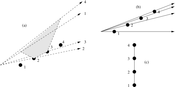
(i) Let and . The four columns of are the four dark points in Figure 1 labeled by their column indices . Figure 1 (a) shows the cone generated by the lifted vectors . The rays generated by the lifted vectors have the same labels as the points that were lifted. Projecting the lower facets of this lifted cone back onto , we get the regular triangulation of shown in Figure 1 (b). The same triangulation is shown as a triangulation of in Figure 1 (c). The faces of the triangulation are and . Using only the maximal faces, we may write .
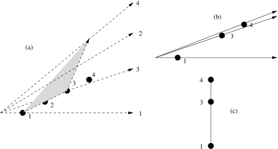
(ii) For the in (i), has four distinct regular triangulations as varies. For instance, the cost vector induces the regular triangulation shown in Figure 2 (b) and (c). Notice that is not a face of .
(iii) If and , then However, in this case, can only be seen as a triangulation of and not of . ∎
For a vector , let denote the support of . The significance of regular triangulations for linear programming is summarized in the following proposition.
Proposition 2.3.
[37, Lemma 1.4] An optimal solution of is any feasible solution such that where is the smallest face of the regular triangulation such that .
Proposition 2.3 implies that is a maximal face of if and only if is an optimal basis for all with in . For instance, in Example 2.2 (i), if then the optimal basis of is where as if , then the optimal solution of is degenerate and either or could be the optimal basis of the linear program. (Recall that is the th column of .) All programs in have one of or as its optimal basis.
Given a polyhedron and a face of , the normal cone of at is the cone . The normal cones of all faces of form a cone complex in called the normal fan of .
Proposition 2.4.
The regular triangulation of is the normal fan of the polyhedron .
Proof.
The polyhedron is the feasible region of , the dual program to . The support of the normal fan of is , since this is the polar cone of the recession cone of . Suppose is any vector in the interior of a maximal face of . Then by Proposition 2.3, has an optimal solution with support . By complementary slackness, the optimal solution to the dual of satisfies for all and otherwise. Since is a maximal face of , for all . Thus is unique, and is contained in the normal cone of at the vertex . If lies in the interior of another maximal face then , (the dual optimal solution to ) satisfies and where . As a result, is distinct from , and each maximal cone in lies in a distinct maximal cone in the normal fan of . Since and the normal fan of are both cone complexes with the same support, they must therefore coincide. ∎
Example 2.2 continued.
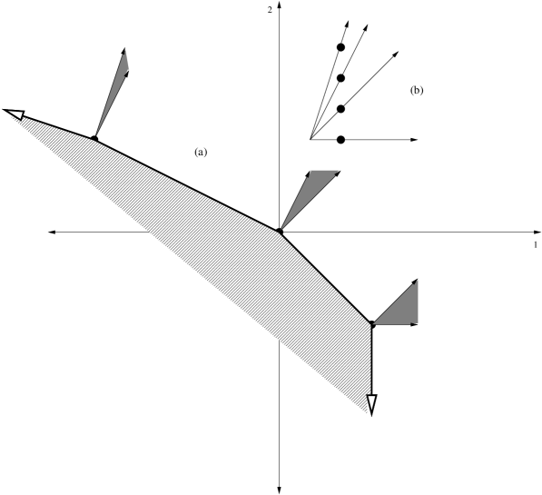
Figure 3 (a) shows the polyhedron for
Example 2.2 (i) with all its normal cones. The normal
fan of is drawn in Figure 3 (b). Compare this fan with
that in Figure 1 (b). ∎
Corollary 2.5.
The polyhedron is simple if and only if the regular subdivision is a triangulation of .
Regular triangulations were introduced by Gel’fand, Kapranov and Zelevinsky [12] and have various applications. They have played a central role in the algebraic study of integer programming ([36], [37]), and we use them now to define group relaxations of .
A subset of partitions as and where consists of the variables indexed by and the variables indexed by the complementary set . Similarly, the matrix is partitioned as and the cost vector as . If is a maximal face of , then is nonsingular and can be written as . Then . Let and, for any face of , let be the extension of to a vector in by adding zeros.
We now define a group relaxation of with respect to each face of .
Definition 2.6.
The group relaxation of the integer program with respect to the face of is the program:
Equivalently, where is the lattice generated by the columns of . Suppose is an optimal solution to the latter formulation. Since is a face of , the columns of are linearly independent, and therefore the linear system has a unique solution. Solving this system for , the optimal solution of can be uniquely lifted to the solution of . The formulation of in Definition 2.6 shows that is an integer vector. The group relaxation solves if and only if is also non-negative.
The group relaxations of from Definition 2.6 contain among them the classical group relaxations of found in the literature. The program , where is the optimal basis of the linear relaxation , is precisely Gomory’s group relaxation of [13]. The set of relaxations as varies among the subsets of this are the extended group relaxations of defined by Wolsey [42]. Since , is a group relaxation of , and hence will certainly be solved by one of its extended group relaxations. However, it is possible to construct examples where a group relaxation solves , but is neither Gomory’s group relaxation of nor one of its nontrivial extended Wolsey relaxations (see Example 4.2). Thus, Definition 2.6 typically creates more group relaxations for each program in than in the classical situation. This has the obvious advantage that it increases the chance that will be solved by some non-trivial relaxation, although one may have to keep track of many more relaxations for each program. In Theorem 2.8, we will prove that Definition 2.6 is the best possible in the sense that the relaxations of defined there are precisely all the bounded group relaxations of the program.
The goal in the rest of this section is to describe a useful reformulation of the group problem which is needed in the rest of the paper and in the proof of Theorem 2.8. Given a sublattice of , a cost vector and a vector , the lattice program defined by this data is
Let denote the -dimensional saturated lattice and be a feasible solution of the integer program . Since can be rewritten as , is equivalent to the lattice program
For , let be the
projection map from
that kills all coordinates indexed by . Then is a sublattice of that is isomorphic to : Clearly, is a surjection. If
for , then
, implies that . Then since the columns of
are linearly independent. Using this fact,
can also be reformulated as a lattice program:
Lattice programs were shown to be solved by Gröbner bases in [39]. Theorem 5.3 in [39] gives a geometric interpretation of these Gröbner bases in terms of corner polyhedra. This paper was the first to make a connection between the theory of group relaxations and commutative algebra (see [39, §6]). Special results are possible when the sublattice is of finite index. In particular, the associated Gröbner bases are easier to compute.
Since the -dimensional lattice is isomorphic to for , is of finite index if and only if is a maximal face of . Hence the group relaxations as varies over the maximal faces of are the easiest to solve among all group relaxations of . They contain among them Gomory’s group relaxation of . We give them a collective name in the following definition.
Definition 2.7.
The group relaxations of , as varies among the maximal faces of , are called the Gomory relaxations of .
It is useful to reformulate once again as follows. Let
be any matrix such that the columns
of generate the lattice , and let be a feasible
solution of as before. Then
The last problem is equivalent to and, therefore
is equivalent to the problem
| (4) |
There is a bijection between the set of feasible solutions of (4) and the set of feasible solutions of via the isomorphism . In particular, is feasible for (4) and it is the pre-image of under this map.
If denotes the submatrix of obtained by deleting the rows indexed by , then . Using the same techniques as above, can be reformulated as
Since for any maximal face of containing and the support of is contained in , since . Hence is equivalent to
| (5) |
The feasible solutions to (4) are the lattice points in the rational polyhedron , and the feasible solutions to (5) are the lattice points in the relaxation of obtained by deleting the inequalities indexed by . In theory, one could define group relaxations of with respect to any . The following theorem illustrates the completeness of Definition 2.6.
Theorem 2.8.
The group relaxation of has a finite optimal solution if and only if is a face of .
Proof.
Since all data are integral it suffices to prove that the linear relaxation
is bounded if and only if .
If is a face of then there exists such that and . Using the fact that we see that . This implies that is a positive linear combination of the rows of since . Hence lies in the polar of which is the recession cone of proving that the linear program is bounded.
The linear program is feasible since is a feasible solution. If it is bounded as well then is feasible and bounded. As a result, the dual of the latter program is feasible. This shows that a superset of is a face of which implies that since is a triangulation. ∎
3. Associated Sets
The group relaxation (seen as (5)) solves the integer program (seen as (4)) if and only if both programs have the same optimal solution . If solves then also solves for every since is a stricter relaxation of than . For the same reason, one would expect that is easier to solve than . Therefore, the most useful group relaxations of are those indexed by the maximal elements in the subcomplex of consisting of all faces such that solves . The following definition isolates such relaxations.
Definition 3.1.
A face of the regular triangulation is an associated set of (or is associated to ) if for some , solves but does not for all faces of such that .
The associated sets of carry all the information about all the group relaxations needed to solve the programs in . In this section we will develop tools to understand these sets. We start by considering the set of all the optimal solutions of all programs in . A basic result in the algebraic study of integer programming is that is an order ideal or down set in , i.e., if and , then . One way to prove this is to show that the complement has the property that if then . Every lattice point in is a feasible solution to a unique program in ( is feasible for ). Hence, is the set of all non-optimal solutions of all programs in . A set with the property that whenever has a finite set of minimal elements. Hence there exists such that
As a result, is completely specified by the finitely many “generators” of its complement . See [40] for proofs of these assertions.
Example 3.2.
Consider the family of knapsack problems:
as varies in the semigroup . The set is generated by the vectors
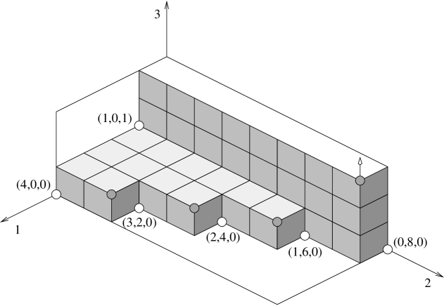
which means that Figure 4 is a picture of (created by Ezra Miller). The white points are its generators. One can see that consists of finitely many points of the form where and the eight “lattice lines” of points , .
∎
For the purpose of computations, it is most effective to think of and algebraically. A monomial in the polynomial ring is a product where . We assume that is a field, say the set of rational numbers. For a scalar and a monomial in , we call a term of . A polynomial in is a combination of finitely many terms in . A subset of is an ideal of if (1) is closed under addition, i.e., and (2) if and then . We say that is generated by the polynomials , denoted as , if . By Hilbert’s basis theorem, every ideal in has a finite generating set. An ideal in is called a monomial ideal if it is generated by monomials, i.e., for monomials in . The monomials that do not lie in are called the standard monomials of . The cost of a term with respect to a vector is the dot product . The initial term of a polynomial with respect to , denoted as , is the sum of all terms in of maximal cost. For any ideal , the initial ideal of with respect to , denoted as , is the ideal generated by all the initial terms of all polynomials in . These concepts come from the theory of Gröbner bases for polynomial ideals. See [9] for an introduction.
The toric ideal of the matrix , denoted as , is the binomial ideal in defined as:
Toric ideals provide the link between integer programming and Gröbner basis theory. See [36] and [41] for an introduction to this area of research. This connection yields the following basic facts that we state without proofs. (Recall that the cost vector of was assumed to be generic in the sense that each program in has a unique optimal solution.)
Lemma 3.3.
[36]
(i) If is generic, then the initial ideal is a
monomial ideal.
(ii) A lattice point is non-optimal for the integer program
, or equivalently, , if and only
if lies in the initial ideal . In other words, a
lattice point lies in if and only if is a
standard monomial of .
(iii) The reduced Gröbner basis of with
respect to is the unique minimal test set for the family of
integer programs .
(iv) If is a feasible solution of , and
is the unique normal form of with respect
to , then is the optimal solution of
.
We do not elaborate on parts (iii) and (iv) of
Lemma 3.3. They are not needed for what follows and are
included for completeness. Since is generic,
Lemma 3.3 (ii) implies that there is a bijection
between the lattice points of and the semigroup
via the map such that . The inverse of sends a vector to the optimal solution of .
Example 3.2 continued. In this example, the toric ideal and its initial ideal with respect to the cost vector is
Note that
the exponent vectors of the generators of are
the generators of . ∎
We will now describe a certain decomposition of the set which in turn will shed light on the associated sets of . For , consider and its relaxation where are as in (4) and (5) and . By Theorem 2.8, both and are polytopes. Notice that if for two distinct vectors , then .
Lemma 3.4.
(i) A lattice point is in if and only
if .
(ii) If , then the group relaxation
solves the integer program if and only if .
Proof.
(i) The lattice point belongs to if and only if is the optimal solution to which is equivalent to being the optimal solution to the reformulation (4) of . Since is generic, the last statement is equivalent to . The second statement follows from (i) and the fact that (5) solves (4) if and only if they have the same optimal solution. ∎
In order to state the coming results, it is convenient to assume that the vector in (4) and (5) is the optimal solution to . For an element and a face of let be the affine semigroup where denotes the th unit vector of . Note that is not a semigroup if (since ), but is a translation of the semigroup . We use the adjective affine here as in an affine subspace which is not a subspace but the translation of one. Note that if , then .
Lemma 3.5.
For and a face of , the affine semigroup is contained in if and only if solves .
Proof.
Suppose . Then by Lemma 3.4 (i), for all ,
Since can be any vector in , . Hence, by Lemma 3.4 (ii), solves .
If , then , and hence . Therefore, if solves , then for all . Since is a relaxation of , for all and hence by Lemma 3.4 (i), . ∎
Lemma 3.6.
For and a face of , solves if and only if solves for all .
Proof.
If and solves , then as seen before, for all . By Lemma 3.4 (ii), solves for all . The converse holds for the trivial reason that . ∎
Corollary 3.7.
For and a face of , the affine semigroup is contained in if and only if solves for all .
Definition 3.8.
For and ,
is called an admissible pair of if
(i) the support of is contained in , and
(ii) or equivalently,
solves for all .
An admissible pair is a standard pair of if the affine semigroup is not properly contained
in where is another admissible pair of
.
Definition 3.9.
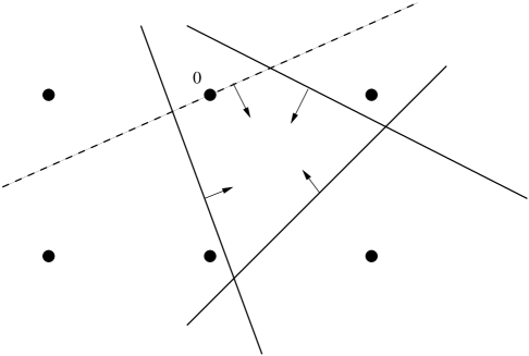
For a face of and a lattice point , we say that the polytope is a standard polytope of if and every relaxation of obtained by removing an inequality in contains a non-zero lattice point.
Figure 5 is a diagram of a standard polytope . The dashed line is the boundary of the half space while the other lines are the boundaries of the halfspaces given by the inequalities in . The origin is the only lattice point in the polytope and if any inequality in is removed, a lattice point will enter the relaxation.
We re-emphasize that if is a standard polytope, then is the same standard polytope if . Hence the same standard polytope can be indexed by infinitely many . We now state the main result of this section which characterizes associated sets in terms of standard pairs and standard polytopes.
Theorem 3.10.
The following statements are equivalent:
(i) The admissible pair is a standard pair of .
(ii) The polytope is a standard polytope of
.
(iii) The face of is associated to .
Proof.
: The admissible pair is standard if and only if for every , there
exists some positive integer and a vector such
that . (If this condition did not hold
for some , then would be an
admissible pair of such that
contains where is obtained from by setting the
th component of to zero. Conversely, if the condition holds for
an admissible pair then the pair is standard.) Equivalently, for each
, there exists a positive integer and a such that contains at least two lattice points. In other words, the
removal of the inequality indexed by from the inequalities in
will bring an extra lattice point
into the corresponding relaxation of . This is
equivalent to saying that is a standard polytope of
.
: Suppose is a standard pair of . Then and solves by Lemma 3.5. Suppose solves for some face such that . Lemma 3.5 then implies that lies in . This contradicts the fact that was a standard pair of since is properly contained in corresponding to the admissible pair where is obtained from by setting for all .
To prove the converse, suppose is associated to . Then there exists some such that solves but does not for all faces of containing . Let be the unique optimal solution of . By Lemma 3.5, . Let be obtained from by setting for all . Then solves since . Hence and is an admissible pair of . Suppose there exists another admissible pair such that . Then . If then and are both orthogonal translates of and hence cannot be properly contained in . Therefore, is a proper subset of which implies that . Then, by Lemma 3.5, solves which contradicts that was an associated set of . ∎
Example 3.2 continued. In Example 3.2 we can choose to be the matrix
The standard polytope defined by the standard pair is hence
while the standard polytope defined by the standard pair is
The associated sets of in this example are and
. There are twelve quadrangular and eight triangular
standard polytopes for this family of knapsack problems. ∎
Standard polytopes were introduced in [22], and the equivalence of parts (i) and (ii) of Theorem 3.10 was proved in [22, Theorem 2.5]. Under the linear map where , the affine semigroup where is a standard pair of maps to the affine semigroup in . Since every integer program in is solved by one of its group relaxations, is covered by the affine semigroups corresponding to its standard pairs. We call this cover and its image in under the standard pair decompositions of and , respectively. Since standard pairs of are determined by the standard polytopes of , the standard pair decomposition of is unique. The terminology used above has its origins in [38] which introduced the standard pair decomposition of a monomial ideal. The specialization to integer programming appear in [22], [23] and [36, §12.D]. The following theorem shows how the standard pair decomposition of dictates which group relaxations solve which programs in .
Theorem 3.11.
Let be the optimal solution of the integer program . Then the group relaxation solves if and only if there is some standard pair of with such that belongs to the affine semigroup .
Proof.
Suppose lies in corresponding to the standard pair of . Then which implies that solves by Lemma 3.5. Hence also solves for all .
To prove the converse, suppose is a maximal element in the subcomplex of all faces of such that solves . Then is an associated set of . In the proof of in Theorem 3.10, we showed that is a standard pair of where is obtained from by setting for all . Then . ∎
Example 3.2 continued. The eight standard pairs of of the form , map to the eight affine semigroups:
contained in . For all right hand side vectors in the union of these sets, the integer program can be solved by the group relaxation . The twelve standard pairs of the from map to the remaining finitely many points
of . If is one of these points, then can
only be solved as the full integer program. In this example, the
regular triangulation . Hence is
a Gomory relaxation of . ∎
For most , the program is solved by one of its Gomory relaxations, or equivalently, by Theorem 3.11, the optimal solution of lies in for some standard pair where is a maximal face of . For mathematical versions of this informal statement, see [36, Proposition 12.16] and [13, Theorems 1 and 2]. Roughly speaking, these right hand sides are away from the boundary of . (This was seen in Example 3.2 above, where for all but twelve right hand sides, was solvable by the Gomory relaxation . Further, these right hand sides were toward the boundary of , the origin in this one-dimensional case.) For the remaining right hand sides, can only be solved by where is a lower dimensional face of - possibly even the empty face. An important contribution of the algebraic approach here is the identification of the minimal set of group relaxations needed to solve all programs in the family and of the particular relaxations necessary to solve any given program in the family.
4. Arithmetic Degree
For an associated set of there are only finitely many standard pairs of indexed by since there are only finitely many standard polytopes of the form . Borrowing terminology from [38], we call the number of standard pairs of the form the multiplicity of in (abbreviated as ). The total number of standard pairs of is called the arithmetic degree of . Our main goal in this section is to provide bounds for these invariants of the the family and discuss their relevance. We will need the following interpretation from Section 3.
Corollary 4.1.
The multiplicity of the face of in is the number of distinct standard polytopes of indexed by , and the arithmetic degree of is the total number of standard polytopes of .
Proof.
This result follows from Theorem 3.10. ∎
Example 3.2 continued.
The multiplicity of the associated set is eight while the
empty set has multiplicity twelve. The arithmetic degree of is hence twenty. ∎
If the standard pair decomposition of is known, then we can solve all programs in by solving (arithmetic degree)-many linear systems as follows. For a given and a standard pair , consider the linear system
| (6) |
As is a face of , this linear system can be solved uniquely for . Since the optimal solution of lies in for some standard pair of , at least one non-negative and integral solution for will be found as we solve the linear systems (6) obtained by varying over all the standard pairs of . If the standard pair yields such a solution , then is the optimal solution of . This pre-processing of has the same flavor as [27]. The main result in [27] is that given a coefficient matrix and cost vector , there exists floor functions such that for a right hand side vector , the optimal solution of the corresponding integer program is the one among that is feasible and attains the best objective function value. The crucial point is that this algorithm runs in time bounded above by a polynomial in the length of the data for fixed and , where is the affine dimension of the space of right hand sides. Given this result, it is interesting to bound arithmetic degree.
The second equation in (6) suggests that one could think of the first arguments in the standard pairs of as “correction vectors” that need to be applied to find the optimal solutions of programs in . Thus the arithmetic degree of is the total number of correction vectors that are needed to solve all programs in . The multiplicities of associated sets give a finer count of these correction vectors, organized by faces of . If the optimal solution of lies in the affine semigroup given by the standard pair of , then is a correction vector for this as well as all other ’s in . One obtains all correction vectors for by solving the (arithmetic degree)-many integer programs with right hand sides for all standard pairs of . See [44] for a similar result from the classical theory of group relaxations.
In Example 3.2, and both its faces and are associated to . In general, not all faces of need be associated sets of and the poset of associated sets can be quite complicated. (We will study this poset in Section 5.) Hence, for , unless is an associated set of . We will now prove that all maximal faces of are associated sets of . Further, if is a maximal face of then is the absolute value of divided by the g.c.d. of the maximal minors of . This g.c.d is non-zero since has full row rank. If the columns of span an affine hyperplane, then the absolute value of divided by the g.c.d. of the maximal minors of is called the normalized volume of the face in . We first give a non-trivial example.
Example 4.2.
Consider the rank three matrix
and the generic cost vector . The first three columns of generate which is simplicial. The regular triangulation
is shown in Figure 6 as a triangulation of . The six columns of have been labeled by their column indices. The arithmetic degree of in this example is . The following table shows all the standard pairs organized by associated sets and the multiplicity of each associated set. Note that all maximal faces of are associated to . The g.c.d. of the maximal minors of is five. Check that is the normalized volume of whenever is a maximal face of .

Observe that the integer program where is solved by with .
By Proposition 2.3, Gomory’s relaxation of is
indexed by since lies in the interior of the
face of . However, neither this
relaxation nor any nontrivial extended relaxation solves
since the optimal solution is not covered by any
standard pair where is a non-empty subset of
.
∎
Theorem 4.3.
For a set , is a standard pair of if and only if is a maximal face of .
Proof.
If is a maximal face of , then by Definition 2.1, there exists such that and . Then and Hence there is a positive dependence relation among and the rows of . Since is a maximal face of , . However, which implies that . Therefore, and the rows of span positively. This implies that is a polytope consisting of just the origin. If any inequality defining this simplex is dropped, the resulting relaxation is unbounded as only inequalities would remain. Hence is a standard polytope of and by Theorem 3.10, is a standard pair of .
Conversely, if is a standard pair of then is a standard polytope of . Since every inequality in the definition of gives a halfspace containing the origin and is a polytope, . Hence there is a positive linear dependence relation among and the rows of . If , then would coincide with the relaxation obtained by dropping some inequality from those in . This would contradict that was a standard polytope and hence and is a maximal face of . ∎
Corollary 4.4.
Every maximal face of is an associated set of .
For Theorem 4.5 and Corollary 4.6 below we assume that the g.c.d. of the maximal minors of is one which implies that .
Theorem 4.5.
If is a maximal face of then the multiplicity of in is .
Proof.
Consider the full dimensional lattice in . Since the g.c.d. of the maximal minors of is assumed to be one, the lattice has index in . Since is full dimensional, it has a strictly positive element which guarantees that each equivalence class of modulo has a non-negative member. This implies that there are distinct equivalence classes of modulo . Recall that if is a feasible solution to then
Since there are equivalence classes of modulo , there are distinct group relaxations indexed by . The optimal solution of each program becomes the right hand side vector of a standard polytope (simplex) of indexed by . Since no two optimal solutions are the same (as they come from different equivalence classes of modulo ), there are precisely standard polytopes of indexed by . ∎
Corollary 4.6.
The arithmetic degree of is bounded below by the sum of the absolute values of as varies among the maximal faces of .
A primary ideal in is a proper ideal such that implies either or for some positive integer . A prime ideal of is a proper ideal such that implies that either or . A primary decomposition of an ideal in is an expression of as a finite intersection of primary ideals in . Lemma 3.3 in [38] shows that every monomial ideal in admits a primary decomposition into irreducible primary ideals that are indexed by the standard pairs of . The radical of an ideal is the ideal . Radicals of primary ideals are prime. The radicals of the primary ideals in a minimal primary decomposition of an ideal are called the associated primes of . This list of prime ideals is independent of the primary decomposition of the ideal. The minimal elements among the associated primes of are called the minimal primes of while the others are called the embedded primes of . The minimal primes of are precisely the defining ideals of the isolated components of the zero-set or variety of while the embedded primes cut out embedded subvarieties in the isolated components. See a textbook in commutative algebra like [10] for more details.
A face of is an associated set of if and only if the monomial prime ideal is an associated prime of the ideal . Further, is a minimal prime of if and only if is a maximal face of . Hence the lower dimensional associated sets of index the embedded primes of . The standard pair decomposition of a monomial ideal was introduced in [38] to study its associated primes. The multiplicity of an associated prime of is an algebraic invariant of , and [38] shows that this is exactly the number of standard pairs indexed by . Similarly, the arithmetic degree of is a refinement of the geometric notion of degree and [38] shows that this number is the total number of standard pairs of . These connections explain our choice of terminology. Theorem 4.3 is a translation of the specialization of Lemma 3.5 in [38] to toric initial ideals. We refer the interested reader to [36, §8 and §12.D] and [38, §3] for the algebraic connections. Theorem 4.5 is a staple result of toric geometry and also follows from [13, Theorem 1]. It is proved via the algebraic technique of localization in [36, Theorem 8.8].
Theorem 4.5 gives a precise bound on the multiplicity of a maximal associated set of , which in turn provides a lower bound for the arithmetic degree of in Corollary 4.6. No exact result like Theorem 4.5 is known when is a lower dimensional associated set of . Such bounds would provide a bound for the arithmetic degree of . Bounds on the arithmetic degree of a general monomial ideal in terms of its dimension and minimal generators can be found in [38, Theorem 3.1]. One hopes that stronger bounds are possible for toric initial ideals. We close with a first attempt at bounding the arithmetic degree of (under certain non-degeneracy assumptions). This result is due to Ravi Kannan, and its simple arguments are along the lines of proofs in [26] and [28].
Suppose and are fixed and is such that and the removal of any inequality defining will bring in a non-zero lattice point into the relaxation. Let denote the th row of , and and be the maximum and minimum absolute values of the subdeterminants of . We will assume that which is a non-degeneracy condition on the data. We assume this set up in Theorem 4.8 and Lemmas 4.9 and 4.10.
Definition 4.7.
If is a convex set and a non-zero vector in , the width of along , denoted as is .
Note that is invariant under translations of .
Theorem 4.8.
If is as above then
Lemma 4.9.
If is as above then for some , ,
Proof.
Clearly, is bounded since otherwise there would be a non-zero lattice point on an unbounded edge of due to the integrality of all data. Suppose for all rows of . Let be the center of gravity of . Then by a property of the center of gravity, for any , th of the vector from to the reflection of about is also in , i.e., . Fix , and let minimize over . By the definition of width, we then have which implies that
| (7) |
Now implies that
| (8) |
| (9) |
Let be the vector obtained by rounding down all components of . Then where for all , and by (9), which leads to . Since ,
| (10) |
and hence, . Repeating this argument for all rows of , we get that . Similarly, if is the vector obtained by rounding up all components of , then where for all . Then (9) implies that which leads to . Again by (10), and hence . Since , at least one of them is non-zero which contradicts that . ∎
Lemma 4.10.
For any two rows of , .
Proof.
Without loss of generality we may assume that . Since is bounded, is finite. Suppose the minimum of over is attained at . Since translations leave the quantities in the lemma invariant, we may prove the lemma for the body obtained by translating by . Now is minimized over at the origin. By LP duality, there are linearly independent constraints among the defining such that the minimum of subject to just these constraints is attained at 0. After renumbering the inequalities if necessary, assume these constraints are the first . Let
where of course . Then by the above, is a bounded simplex.
Since contains , it suffices to show that for each ,
| (11) |
We show that for each vertex of , which will prove (11). This is clearly true for . Without loss of generality assume that vertex satisfies for . Since the determinant of the submatrix of consisting of the rows is not zero, for any there exists rationals such that . By Cramer’s rule, . Therefore, since for . This proves that
∎
Proof of Theorem 4.8.
From Lemmas 4.9 and 4.10 it follows that for any , , . Since , while . Therefore, and hence, for all .
∎
Reverting back to our set up, let . Suppose is the standard polytope . By Theorem 4.8, .
Corollary 4.11.
If no maximal minor of is zero, then the arithmetic degree of is at most .
The above arguments do not use the condition that the removal of an inequality from will bring in a lattice point into the relaxation. Further, the bound is independent of the number of facets of , and Corollary 4.11 is straightforward. Thus, further improvements may be possible with more effort. However, apart from providing a bound for arithmetic degree, these proofs have the nice feature that they build a bridge to techniques from the geometry of numbers that have played a central role in theoretical integer programming as seen in the work of Kannan, Lenstra, Lovász, Scarf and others. See [29] for a survey.
5. The Chain Theorem
We now examine the structure of the poset of associated sets of which we denote as . All elements of are faces of the regular triangulation and the partial order is set inclusion. Theorem 4.3 provides a first result.
Corollary 5.1.
The maximal elements of are the maximal faces of .
Example 4.2 continued.
The lower dimensional associated sets of this example (except the
empty set) are the thick faces of shown in Figure 7.
∎

Despite the seemingly chaotic structure of beyond its maximal elements, it has an important structural property that we now explain.
Theorem 5.2.
[The Chain Theorem] If is an associated set of and then there exists a face that is also an associated set of with the property that and .
Proof.
Since is an associated set of , by Theorem 3.10, has a standard pair of the form and is a standard polytope of . Since , is not a maximal face of and hence by Theorem 4.3, . For each , let be the relaxation of obtained by removing the th inequality from , i.e.,
Let . Clearly, , and, since the removal of introduces at least one lattice point into , . Let be the optimal solution to if the program is bounded. This integer program is always feasible since , but it may not have a finite optimal value. However, there exists at least one for which the above integer program is bounded. To see this, pick a maximal simplex such that . The polytope is a simplex and hence bounded. This polytope contains all for , and hence all these are bounded and have finite optima with respect to . We may assume that the inequalities in are labeled so that the finite optimal values are ordered as where .
Claim: Let . Then is the unique lattice point in and the removal of any inequality from will bring in a new lattice point into the relaxation.
Proof. Since lies in , . However, since otherwise,
both and would be optimal solutions to contradicting that is
generic. Therefore,
Since is generic, is the unique lattice point in the
first polytope and the second polytope is free of lattice points.
Hence is the unique lattice point in . The relaxation
of got by removing is the polyhedron
for and .
Either this is unbounded, in which case there is a lattice point
in this relaxation such that ,
or (if ) we have and lies in this relaxation.
Translating by we get where since is feasible for all inequalities except the first one. Now , and hence is a standard pair of . ∎
Example 4.2 continued.
The empty set is associated to and is a saturated chain in
that starts at the empty set. ∎
In algebraic language, the chain theorem says that the associated primes of occur in saturated chains. This was proved in [22, Theorem 3.1]. When the cost vector is not generic, is no longer a monomial ideal, and its associated primes need not come in saturated chains. See [22, Remark 3.3] for such an example. An important open question in the algebraic study of integer programming is to characterize all monomial ideals that can appear as the initial ideal (with respect to some generic cost vector) of a toric ideal. In our set up this amounts to characterizing all down sets in that can appear as the set of optimal solutions to a family , where and satisfy the assumptions from Section 2. Theorem 5.2 imposes the necessary condition that the poset of sets indexing the standard pairs of the down set have the chain property. Unfortunately, this is not sufficient to characterize down sets of the form . See [30] for another class of monomial ideals that also have the chain property.
Since the elements of are faces of , a maximal face of which is a -element set, the length of a maximal chain in is at most . We denote the maximal length of a chain in by . When (the corank of ) is small compared to , has a stronger upper bound than . We use the following result of Bell and Scarf to prove the bound.
Theorem 5.3.
[33, Corollary 16.5 a] Let be a system of linear inequalities in variables, and let . If max is a finite number, then max = max for some subsystem of with at most inequalities.
Theorem 5.4.
The length of a maximal chain in the poset of associated sets of is at most .
Proof.
As seen earlier, . If lies in , then the origin is the optimal solution to the integer program By Theorem 5.3, we need at most inequalities to describe the same integer program which means that we can remove at least inequalities from without changing the optimum. Assuming that the inequalities removed are indexed by , will be a standard polytope of . Therefore, . This implies that the maximal length of a chain in is at most . ∎
Corollary 5.5.
The cardinality of an associated set of is at least .
Corollary 5.6.
If , then .
Proof.
In this situation, . ∎
We conclude this section with a family of examples for which . This is adapted from [22, Proposition 3.9] which was modeled on a family of examples from [32].
Proposition 5.7.
For each , there is an integer matrix of corank and a cost vector where such that .
Proof.
Given , let be the matrix whose rows are all the -vectors in except . Let be obtained by stacking on top of where is the identity matrix. Set , and . By construction, the columns of span the lattice . We may assume that the first row of is . Adding this row to all other rows of we get with the same row space as . Hence the columns of are also a basis for the lattice . Since the rows of span as a lattice, we can find a cost vector such that .
For each row of set , and let be the vector of all s. By construction, the polytope has no lattice points in its interior, and each of its facets has exactly one vertex of the unit cube in in its relative interior. If we let , then the polytope is a standard polytope of where and . Since a maximal face of is a -element set and , Theorem 5.2 implies that . However, by Theorem 5.4, since by assumption. ∎
6. Gomory Integer Programs
Recall from Definition 2.7 that a group relaxation of is called a Gomory relaxation if is a maximal face of . As discussed in Section 2, these relaxations are the easiest to solve among all relaxations of . Hence it is natural to ask under what conditions on and would all programs in be solvable by Gomory relaxations. We study this question in this section. The majority of the results here are taken from [21].
Definition 6.1.
The family of integer programs is a Gomory family if, for every , is solved by a group relaxation where is a maximal face of the regular triangulation .
Theorem 6.2.
The following conditions are equivalent:
(i) is a Gomory family.
(ii) The associated sets of are precisely the maximal
faces of .
(iii) is a standard pair of if and only
if is a maximal face of .
(iv) All standard polytopes of are simplices.
Proof.
By Definition 6.1, is a Gomory family if and only if for all , can be solved by one of its Gomory relaxations. By Theorem 3.11, this is equivalent to saying that every lies in some where is a maximal face of and a standard pair of . Definition 3.1 then implies that all associated sets of are maximal faces of . By Theorem 4.3, every maximal face of is an associated set of and hence . The equivalence of statements (ii), (iii) and (iv) follow from Theorem 3.10. ∎
If is a generic cost vector such that for a triangulation of , , then we say that supports the order ideal and the family of integer programs . No regular triangulation of the matrix in Example 4.2 supports a Gomory family. Here is a matrix with a Gomory family.
Example 6.3.
Consider the matrix
In this case, has 14 distinct regular triangulations and 48 distinct sets as varies among all generic cost vectors. Ten of these triangulations support Gomory families; one for each triangulation. For instance, if , then
and is a Gomory family since the standard pairs of are:
∎
Algebraically, is a Gomory family if and only if the initial ideal has no embedded primes and hence Theorem 6.2 is a characterization of toric initial ideals without embedded primes. A sufficient condition for an ideal in to not have embedded primes is that it is Cohen-Macaulay [10]. In general, Cohen-Macaulayness is not necessary for an ideal to be free of embedded primes. However, empirical evidence seemed to suggest for a while that for toric initial ideals, Cohen-Macaulayness might be equivalent to being free of embedded primes. A counterexample to this was found recently by Laura Matusevich. The algebraic approach to integer programming allows one to compute all down sets of a fixed matrix as varies among the set of generic cost vectors. See [24], [36] and [37] for details. The software package TiGERS [2] is custom-tailored for this purpose.
We now compare the notion of a Gomory family to the classical notion of total dual integrality [33, §22]. It will be convenient to assume that for these results.
Definition 6.4.
The system is totally dual integral (TDI) if has an integral optimal solution for each .
Definition 6.5.
The regular triangulation is unimodular if for every maximal face .
Example 6.6.
Lemma 6.7.
The system is TDI if and only if the regular triangulation is unimodular.
Proof.
Corollary 8.4 in [36] shows that is unimodular if and only if the monomial ideal is generated by square-free monomials. Hence, by computing , one can determine whether is TDI. Such computations can be carried out on computer algebra systems like CoCoA [1] or MACAULAY 2 [18] for moderately sized examples. See [36] for algorithms. Standard pair decompositions of monomial ideals can be computed with MACAULAY 2 [20].
Theorem 6.8.
If is TDI then is a Gomory family.
Proof.
By Theorem 4.3, is a standard pair of for every maximal face of . Lemma 6.7 implies that is unimodular (i.e., ), and therefore for every maximal face of . Hence the semigroups arising from the standard pairs as varies over the maximal faces of cover . Therefore the only standard pairs of are as varies over the maximal faces of . The result then follows from Theorem 6.2. ∎
When is TDI, the multiplicity of a maximal face of in is one (from Theorem 4.5). By Theorem 6.8, no lower dimensional face of is associated to . While this is sufficient for to be a Gomory family, it is far from necessary. TDI-ness guarantees local integrality in the sense that has an integral optimum for every integral in . In contrast, if is a Gomory family, the linear optima of the programs in may not be integral.
If is unimodular (i.e., for every nonsingular maximal submatrix of ), then the feasible regions of the linear programs in have integral vertices for each , and is TDI for all . Hence if is unimodular, then is a Gomory family for all generic cost vectors . However, just as integrality of the optimal solutions of programs in is not necessary for to be a Gomory family, unimodularity of is not necessary for to be a Gomory family for all .
Example 6.9.
Consider the seven by twelve integer matrix
of rank seven. The maximal minors of have absolute values zero,
one and two and hence is not unimodular. This matrix has
distinct regular triangulations supporting distinct order ideals
(computed using TiGERS). In each case, the standard pairs
of are indexed by just the maximal simplices of the
regular triangulation that supports it. Hence is
a Gomory family for all generic . ∎
The above discussion shows that being a Gomory family is more general than being TDI. Similarly, being a Gomory family for all generic is more general than being a unimodular matrix.
7. Gomory Families and Hilbert Bases
As we just saw, unimodular matrices or more generally, unimodular regular triangulations lead to Gomory families. A common property of unimodular matrices and matrices such that has a unimodular triangulation is that the columns of form a Hilbert basis for , i.e., (assuming ).
Definition 7.1.
A integer matrix is normal if the semigroup equals .
The reason for this (highly over used) terminology here is that if the columns of form a Hilbert basis, then the zero set of the toric ideal (called a toric variety) is a normal variety. See [36, Chapter 14] for more details. We first note that if is not normal, then need not be a Gomory family for any cost vector .
Example 7.2.
The matrix is not normal since which lies in cannot be written as a non-negative integer combination of the columns of . This matrix gives rise to 10 distinct order ideals supported on its four regular triangulations and . Each has at least one standard pair that is indexed by a lower dimensional face of .
The matrix in Example 4.2 is also not normal and has no Gomory families. While we do not know whether normality of is sufficient for the existence of a generic cost vector such that is a Gomory family, we will now show that under certain additional conditions, normal matrices do give rise to Gomory families.
Definition 7.3.
A integer matrix is -normal if has a triangulation such that for every maximal face , the columns of in form a Hilbert basis.
Remark 7.4.
If is -normal for some triangulation , then it is normal. To see this note that every lattice point in lies in for some maximal face . Since is -normal, this lattice point also lies in the semigroup generated by the columns of in and hence in .
Observe that is -normal with respect to all the unimodular triangulations of . Hence triangulations with respect to which is -normal generalize unimodular triangulations of .
Examples 7.5 and 7.6 show that the set of matrices where has a unimodular triangulation is a proper subset of the set of -normal matrices which in turn is a proper subset of the set of normal matrices.
Example 7.5.
Examples of normal matrices with no unimodular triangulations can be found in [6] and [11]. If is simplicial for such a matrix, will be -normal with respect to its coarsest (regular) triangulation consisting of the single maximal face with support . For instance, consider the following example taken from [11]:
Here has regular triangulations and no unimodular triangulations. Since is simplicial, is -normal with respect to its coarsest regular triangulation .
Example 7.6.
There are normal matrices that are not -normal with respect to any triangulation of . To see such an example, consider the following modification of the matrix in Example 7.5 that appears in [36, Example 13.17] :
This matrix is again normal and each of its nine columns generate an extreme ray of . Hence the only way for this matrix to be -normal for some would be if is a unimodular triangulation of . However, there are no unimodular triangulations in this example.
Theorem 7.7.
If is -normal for some regular triangulation then there exists a generic cost vector such that and is a Gomory family.
Proof.
Without loss of generality we can assume that the columns of in form a minimal Hilbert basis for every maximal face of . If there were a redundant element, the smaller matrix obtained by removing this column from would still be -normal.
For a maximal face , let be the set of indices of all columns of lying in that are different from the columns of . Suppose are the columns of that generate the one dimensional faces of , and a cost vector such that . We modify to obtain a new cost vector such that as follows. For , let . If for some maximal face , then , and we define . Hence, for all , lies in which was a facet of . If is a vector as in Definition 2.1 showing that is a maximal face of then for all and otherwise. Since , we conclude that is a maximal face of .
If lies in for a maximal face , then has at least one feasible solution with support in since is -normal. Further, lies in and all feasible solutions of with support in have the same cost value by construction. Suppose is any feasible solution of with support not in . Then since if and only if and is a lower facet of . Hence the optimal solutions of are precisely those feasible solutions with support in . The vector can be expressed as where are unique and is also unique. The vector where . Setting for all , for all and otherwise, we obtain all feasible solutions of with support in .
If there is more than one such feasible solution, then is not generic. In this case, we can perturb to a generic cost vector by choosing , whenever and otherwise. Suppose are the optimal solutions of the integer programs where . (Note that is the index of in .) The support of each such is contained in . For any , the optimal solution of is hence for some and with support in . This shows that is covered by the affine semigroups where is a maximal face of and as above for each . By construction, the corresponding admissible pairs are all standard for . Since all data is integral, and hence can be scaled to lie in . Renaming as , we conclude that is a Gomory family. ∎
Corollary 7.8.
Let be a normal matrix such that is simplicial, and let be the coarsest triangulation whose single maximal face has support . Then there exists a cost vector such that and is a Gomory family.
Example 7.9.
Consider the normal matrix in Example 6.3. Here is generated by the first, second and sixth columns of and hence is -normal with respect to the regular triangulation . There are 13 distinct sets supported on . Among the 13 corresponding families of integer programs, only one is a Gomory family. A representative cost vector for this is . The standard pair decomposition of is the one constructed in Theorem 7.7. The affine semigroups from this decomposition are:
Note that is not -normal
with respect to the regular triangulation supporting the Gomory family
in Example 6.3. The columns of
in are the columns of and .
The vector is in the minimal Hilbert basis of
but is not a column of . This example shows
that a regular triangulation of can support a
Gomory family even if is not -normal. The Gomory families
in Theorem 7.7 have a very special standard pair
decomposition. ∎
Problem 7.10.
If is a normal matrix, does there exist a generic cost vector such that is a Gomory family?
While we do not know the answer to this question, we will now show that stronger results are possible for small values of .
Theorem 7.11.
If is a normal matrix and , then there exists a generic cost vector such that is a Gomory family.
Proof.
Before we proceed, we rephrase Problem 7.10 in terms of covering properties of and along the lines of [6], [7], [8], [11] and [34]. To obtain the same set up as in these papers we assume in this section that is normal and the columns of form the unique minimal Hilbert basis of . Using the terminology in [7], the free Hilbert cover problem asks whether there exists a covering of by semigroups where the columns of are linearly independent. The unimodular Hilbert cover problem asks whether can be covered by full dimensional unimodular subcones (i.e., ), while the stronger unimodular Hilbert partition problem asks whether has a unimodular triangulation. (Note that if has a unimodular Hilbert cover or partition using subcones , then is covered by the semigroups .) All these problems have positive answers if since admits a unimodular Hilbert partition in this case [6], [34]. Normal matrices (with ) such that has no unimodular Hilbert partition can be found in [6] and [11]. Examples (with ) that admit no free Hilbert cover and hence no unimodular Hilbert cover can be found in [7] and [8].
When is TDI, the standard pair decomposition of induced by gives a unimodular Hilbert partition of by Theorem 6.7. An important difference between Problem 7.10 and the Hilbert cover problems is that affine semigroups cannot be used in Hilbert covers. Moreover, affine semigroups that are allowed in standard pair decompositions come from integer programming. If there are no restrictions on the affine semigroups that can be used in a cover, can always be covered by full dimensional affine semigroups: for any triangulation of with maximal subcones , the affine semigroups cover as varies in and varies among the maximal faces of the triangulation. A partition of derived from this idea can be found in [35, Theorem 5.2]. We recall the notion of supernormality introduced in [19].
Definition 7.12.
A matrix is supernormal if for every submatrix of , the columns of that lie in form a Hilbert basis for .
Proposition 7.13.
For , the following are equivalent:
-
(i)
is supernormal,
-
(ii)
is -normal for every regular triangulation of ,
-
(iii)
Every triangulation of in which all columns of generate one dimensional faces is unimodular.
Proof.
The equivalence of (i) and (iii) was established in [19, Proposition 3.1]. Definition 7.12 shows that (i) (ii). Hence we just need to show that (ii) (i). Suppose that is -normal for every regular triangulation of . In order to show that is supernormal we only need to check submatrices where the dimension of is . Choose a cost vector with if the th column of does not generate an extreme ray of , and otherwise. This gives a polyhedral subdivision of in which is a maximal face. There are standard procedures that will refine this subdivision to a regular triangulation of . Let be the set of maximal faces of such that lies in . Since is -normal, the columns of that lie in form a Hilbert basis for for each . However, since their union is the set of columns of that lie in , this union forms a Hilbert basis for . ∎
It is easy to catalog all -normal and supernormal matrices, of the type considered in this paper, for small values of . We say that the matrix is graded if its columns span an affine hyperplane in . If , has triangulations each of which has the unique maximal subcone whose support is . If we assume that , then is normal if and only if either , or . Also, is normal if and only if it is supernormal. If and the columns of are ordered counterclockwise around the origin, then is normal if and only if for all . Such an is supernormal since it is -normal for every triangulation — the Hilbert basis of a maximal subcone of is precisely the set of columns of in that subcone. If then as mentioned before, has a unimodular triangulation with respect to which is -normal. However, not every such needs to be supernormal: the matrix in Example 6.3 is not -normal for the supporting the Gomory family in that example. If and is graded, then without loss of generality we can assume that the columns of span the hyperplane . If is normal as well, then its columns are precisely all the lattice points in the convex hull of . Conversely, every graded normal with arises this way — its columns are all the lattice points in a polygon in with integer vertices. In particular, every triangulation of that uses all the columns of is unimodular. Hence, by Proposition 7.13, is supernormal, and therefore -normal for any triangulation of .
Theorem 7.14.
Let be a normal matrix of rank .
-
(i)
If or is graded and , every regular triangulation of supports at least one Gomory family.
-
(ii)
If and is graded, every regular triangulation of supports exactly one Gomory family.
-
(iii)
If and is not graded, or if and is graded, then not all regular triangulations of may support a Gomory family. In particular, may not be -normal with respect to every regular triangulation.
Proof.
(i) If or is graded and , is supernormal and hence by Proposition 7.13 and Theorem 7.7, every regular triangulation of supports at least one Gomory family.
(ii) If and is graded, then we may assume that
In this case, is supernormal and hence every regular triangulation of supports a Gomory family by Theorem 7.7. Suppose the maximal cones of , in counter-clockwise order, are . Assume the columns of are labeled such that for , and the columns of in the interior of are labeled in counter-clockwise order as . Hence the columns of from left to right are:
Indexing the columns of by their labels, the maximal faces of are for . Let be the unit vector of indexed by the true column index of in and be the unit vector of indexed by the true column index of in . Since the columns of form a minimal Hilbert basis of , is the unique solution to for all and is the unique solution to for all . Hence the standard pairs of Theorem 7.7 are and for and .
Suppose supports a second Gomory family . Then every standard pair of is also of the form for , and of them are for . The remaining standard pairs are of the form . To see this, consider the semigroups in arising from the standard pairs of . The total number of standard pairs of and are the same. Since the columns of all lie on , no two s can be covered by a semigroup coming from the same standard pair and none of them are covered by a semigroup . We show that if is a standard pair of then and thus .
If , the standard pairs of are as in Theorem 7.7. If , consider the last cone . If is the second to last column of , then is unimodular and the semigroup from covers . The subcomplex comprised of is a regular triangulation of where is obtained by dropping the last column of . Since is a normal graded matrix with and has less than maximal cones, the standard pairs supported on are as in Theorem 7.7 by induction. If is not the second to last column of then , the second to last column of is in the Hilbert basis of but is not a generator of . So has a standard pair of the form . If , then the lattice point cannot be covered by the semigroup from this or any other standard pair of . Hence . By a similar argument, the remaining standard pairs indexed by are along with . These are precisely the standard pairs of indexed by . Again we are reduced to considering the subcomplex comprised of and by induction, the remaining standard pairs of are as in Theorem 7.7.
(iii) The normal matrix of Example 6.3 has 10 distinct Gomory families supported on 10 out of the 14 regular triangulations of . Furthermore, the normal matrix
has 11 distinct Gomory families supported on 11 out of its 19 regular triangulations. ∎
References
- [1] Cocoa 4.1. Available from ftp://cocoa.dima.unige.it/cocoa.
- [2] TiGERS. Available from http://www.math.washington.edu/thomas/programs.html.
- [3] K. Aardal, R. Weismantel, and L. Wolsey. Non-standard approaches to integer programming. Report UU-CS-1999-41, Department of Computer Science, Utrecht University, 1999.
- [4] D. Bell and J. Shapiro. A convergent duality theory for integer programming. Journal of Operations Research, 25:419–434, 1977.
- [5] L. J. Billera, P. Filliman, and B. Sturmfels. Constructions and complexity of secondary polytopes. Advances in Mathematics, 83:155–179, 1990.
- [6] C. Bouvier and G. Gonzalez-Springberg. Système generateurs minimal, diviseurs essentiels et G-dèsingularizations de vari’et’es toriques. Tôhoku Math. Journal, 46:125–149, 1994.
- [7] W. Bruns and J. Gubeladze. Normality and covering properties of affine semigroups. Journal für die reine und angewandte Mathematik, 510:161–178, 1999.
- [8] W. Bruns, J. Gubeladze, M. Henk, A. Martin, and R. Weismantel. A counterexample to an integer analogue of caratheodory’s theorem. Journal für die reine und angewandte Mathematik, 510:179–185, 1999.
- [9] D. Cox, J. Little, and D. O’Shea. Ideals, Varieties, and Algorithms. Springer-Verlag, New York, 1996. Second edition.
- [10] D. Eisenbud. Commutative Algebra with a View Towards Algebraic Geometry. Springer Graduate Texts in Mathematics, 1994.
- [11] R. Firla and G. Ziegler. Hilbert bases, unimodular triangulations, and binary covers of rational polyhedral cones. Discrete and Computational Geometry, 21:205–216, 1999.
- [12] I. M. Gel’fand, M. Kapranov, and A. Zelevinsky. Multidimensional Determinants, Discriminants and Resultants. Birkhäuser, Boston, 1994.
- [13] R. E. Gomory. On the relation between integer and noninteger solutions to linear programs. Proceedings of the National Academy of Sciences, 53:260–265, 1965.
- [14] R. E. Gomory. Faces of an integer polyhedron. Proceedings of the National Academy of Sciences, 57:16–18, 1967.
- [15] R. E. Gomory. Some polyhedra related to combinatorial problems. Linear Algebra and its Applications, 2:451–558, 1969.
- [16] R. E. Gomory and E.L. Johnson. Some continuous functions related to corner polyhedra. Mathematical Programming, 3:23–85, 1972.
- [17] G. Gorry, W. Northup, and J. Shapiro. Computational experience with a group theoretic integer programming algorithm. Mathematical Programming, 4:171–192, 1973.
- [18] D. Grayson and M. Stillman. Macaulay 2, a software system for research in algebraic geometry. Available at http://www.math.uiuc.edu/Macaulay2.
- [19] S. Hoşten, D. Maclagan, and B. Sturmfels. Supernormal vector configurations. math.CO/0105036.
- [20] S. Hoşten and G. Smith. Monomial ideals. In D. Eisenbud, D. Grayson, M. Stillman, and B. Sturmfels, editors, Mathematical Computations with Macaulay 2. Springer Verlag. To appear.
- [21] S. Hoşten and R.R. Thomas. Gomory integer programs. math.OC/0106031.
- [22] S. Hoşten and R.R. Thomas. The associated primes of initial ideals of lattice ideals. Mathematical Research Letters, 6:83–97, 1999.
- [23] S. Hoşten and R.R. Thomas. Standard pairs and group relaxations in integer programming. Journal of Pure and Applied Algebra, 139:133–157, 1999.
- [24] B. Huber and R.R. Thomas. Computing Gröbner fans of toric ideals. Experimental Mathematics, 9:321–331, 2000.
- [25] E.L. Johnson. Integer Programming: Facets, Subadditivity, and Duality for Group and Semi-group Problems. SIAM CBMS Regional Conference Series in Applied Mathematics No. 32, Philadelphia, 1980.
- [26] R. Kannan. Lattice translates of a polytope and the Frobenius problem. Combinatorica, 12:161–177, 1992.
- [27] R. Kannan. Optimal solution and value of parametric integer programs. In G. Rinaldi and L.Wolsey, editors, Proceedings of the Third IPCO conference, pages 11–21, 1993.
- [28] R. Kannan, L. Lovász, and H.E. Scarf. Shapes of polyhedra. Mathematics of Operations Research, 15:364–380, 1990.
- [29] L. Lovász. Geometry of numbers and integer programming. In M. Iri and K. Tanebe, editors, Mathematical Programming: Recent Developments and Applications, pages 177–210. Kluwer Academic Press, 1989.
- [30] E.N. Miller, B. Sturmfels, and K. Yanagawa. Generic and cogeneric monomial ideals. Journal of Symbolic Computation, 29:691–708, 2000.
- [31] G. Nemhauser and L. Wolsey. Integer and Combinatorial Optimization. Wiley, New York, 1988.
- [32] I. Peeva and B. Sturmfels. Syzygies of codimension 2 lattice ideals. Mathematische Zeitschrift, 229:163–194, 1998.
- [33] A. Schrijver. Theory of Linear and Integer Programming. Wiley-Interscience Series in Discrete Mathematics and Optimization, New York, 1986.
- [34] A. Sebö. Hilbert bases, Caratheodory’s theorem and combinatorial optimization. In R. Kannan and W. Pulleyblank, editors, Integer Programming and Combinatorial Optimization, pages 431–456. University of Waterloo Press, Waterloo, 1990. Mathematical Programming Society.
- [35] R. P. Stanley. Linear diophantine equations and local cohomology. Inventiones Math., 68:175–193, 1982.
- [36] B. Sturmfels. Gröbner Bases and Convex Polytopes. American Mathematical Society, Providence, RI, 1995.
- [37] B. Sturmfels and R. R. Thomas. Variation of cost functions in integer programming. Mathematical Programming, 77:357–387, 1997.
- [38] B. Sturmfels, N. Trung, and W. Vogel. Bounds on projective schemes. Mathematische Annalen, 302:417–432, 1995.
- [39] B. Sturmfels, R. Weismantel, and G. Ziegler. Gröbner bases of lattices, corner polyhedra and integer programming. Beiträge zur Algebra und Geometrie, 36:281–298, 1995.
- [40] R. R. Thomas. A geometric Buchberger algorithm for integer programming. Mathematics of Operations Research, 20:864–884, 1995.
- [41] R. R. Thomas. Applications to integer programming. In D. Cox and B. Sturmfels, editors, Applications of Computational Algebraic Geometry, volume 53, pages 119–142. AMS Proceedings of Symposia in Applied Mathematics, 1997.
- [42] L. Wolsey. Extensions of the group theoretic approach in integer programming. Management Science, 18:74–83, 1971.
- [43] L. Wolsey. Generalized dynamic programming methods in integer programming. Mathematical Programming, 4:222–232, 1973.
- [44] L. Wolsey. The b-hull of an integer program. Discrete Applied Mathematics, 3:193–201, 1981.