Shock-capturing with natural high frequency oscillations

Abstract

This paper explores the potential of a newly developed conjugate filter oscillation reduction (CFOR) scheme for shock-capturing under the influence of natural high-frequency oscillations. The conjugate low-pass and high-pass filters are constructed based on the principle of the discrete singular convolution. Two Euler systems, the advection of an isentropy vortex flow and the interaction of shock-entropy wave are considered to demonstrate the utility of the CFOR scheme. Computational accuracy and order of approximation are examined and compared with the literature. Some of the best numerical results are obtained for the shock-entropy wave interaction. Numerical experiments indicate that the proposed scheme is stable, conservative and reliable for the numerical simulation of hyperbolic conservation laws.

I Introduction

Scientists and engineers often face challenging problems in scientific and engineering computing. Some of typical problems include numerically induced chaos due to initial value being close to homoclinic manifold singularity in nonlinear Hamiltonian systems. Numerical instability in the prediction of higher-order eigenvalues is a long standing obstacle for the progress in the optimization of space structures. In aerodynamics and fluid dynamics, one of major difficulties is to attain solutions that are free of spurious oscillations for compressible Euler equations involving steep gradient at discontinuities. In particular, to construct a high-accuracy and high-resolution solution for a system involving the interaction of shock-turbulent boundary layer is a severe challenge due to its natural high-frequency components. Traditional schemes such as upwind, Riemann solver, approximate Riemann solver, random choice method, artificial viscosity, are usually of low order in nature. More sophisticated approaches, such as total variation diminishing (TVD), essentially non-oscillatory (ENO)[1], weighted essentially non-oscillatory (WENO), characteristic-based-split (CBS)[2] and discontinuous Galerkin schemes[3] are proposed in the past two decades. Generally, these shock-capturing schemes are shown to be very successful in many applications.

Recently, it has been pointed out[4] that the use of a sixth order accurate ENO scheme in the entire computational domain leads to a significant damping of turbulent fluctuations. Garnier et al[5] found that in the framework of freely decaying turbulence, the numerical dissipation of high-order accurate shock-capturing schemes masks the effect of the subgrid-scale model. Therefore, alternative approaches are of pressing desirable for many practical applications. The use of post-processing based filtering is one of important alternative approaches which can overcome the problem of excessive numerical dissipation in many sophisticated shock-capturing schemes. Engquist et al[6] proposed a set of nonlinear filters which discriminate and eliminate the dispersive wiggles in the basic solution. Recently, Garnier et al[7] have reported the use of the nonlinear dissipation components in some high-order shock-capturing schemes, such as the ENO and WENO, as filters. With appropriate sensors, these ENO filters are shown to effectively improve the resolution of density waves, entropy waves and stochastic turbulent fluctuations. Indeed, in the case of direct simulation of turbulence, typical successful numerical approaches are spectral methods for their capability of resolving multiscale features in turbulent fluctuations. However, spectral methods are notorious for their Gibbs’ oscillations at the discontinuity. Therefore, it is highly desirable to have methods that are of (arbitrary) high accuracy for resolving high-frequency waves and stochastic turbulent fluctuations, and are capable of shock-capturing without excessive numerical dissipation.

Conjugate filter oscillation reduction (CFOR)[8, 9] is one of such schemes newly developed for solving practical problems. The CFOR scheme is constructed based on the discrete singular convolution (DSC) algorithm[10, 11, 12], a new approach for the numerical computation of singular convolutions. The theoretical foundation of the DSC algorithm is the theory of distributions and the theory of wavelet analyses. The DSC algorithm provides a unified approach to conventional local and global methods and has controllable accuracy for numerical solution of differential equations. The essential idea in the CFOR scheme is to use conjugate (DSC) low-pass filters to remove the spurious oscillation generated by conjugate (DSC) high-pass filters which are implemented for the numerical approximation of differentiation operators. Conjugate filters are constructed by using DSC kernels and are optimal in the sense that they have similar order of regularity, accuracy, frequency bandwidth and computational supports. The CFOR scheme has been successfully applied to shock-capturing in association with Burgers’ equation, one- and two-dimensional (2D) Euler systems including the Sod and Lax problems, and the Mach 3 flow past a wind tunnel with a step. The most promising feature of the CFOR scheme is that, the approach has controllable order of approximation for shock-capturing under practical situations. The objective of the present work is to explore the utility and limitation of the CFOR scheme in dealing with the problem of shock-high frequency entropy wave interaction, which is very challenging because conventional methods encounter the difficulty of either insufficient accuracy or excessive numerical damping. It is believed that a better understanding of the CFOR scheme is of importance to the development of high-accuracy and low-dissipation schemes for the numerical solution of more challenging problems, such as shock-turbulence interaction.

This paper is organized as follows. A brief retrospection is given to the DSC algorithm and the CFOR scheme in Section II. Section III is devoted to the numerical experiments of 1D and 2D Euler systems, an isentropic vortex flow and the interaction of shock-entropy wave. The latter is designed to test the capability of resolving shock from high-frequency entropy waves. A conclusion ends the paper.

II The DSC algorithm and CFOR scheme

A DSC filters

Singular convolutions occur commonly in science and engineering. Discrete singular convolution (DSC) is an effective approach for the numerical realization of singular convolutions. There are many detailed descriptions about the discrete singular convolution in the literature[10, 11, 12]. The introduction in Ref. [10] is recommended for its theoretical underpinning and approximation philosophy. For the sake of integrity and convenience, a brief review of the DSC algorithm is given before describing the CFOR scheme.

In the context of distribution theory, a singular convolution can be defined by

$$F(t)=(T*\eta)(t)=\int_{-\infty}^{\infty}T(t-x)\eta(x)dx,$$ (1)

where $T$ is a singular kernel and $\eta(x)$ is an element of the space of test functions. Interesting examples include singular kernels of Hilbert (and Abel) type and delta type. The former plays an important role in the theory of analytical functions, processing of analytical signals, theory of linear responses and Radon transform. Since delta type kernels are the key element in the theory of approximation and the numerical solution of differential equations, we focus on the singular kernels of delta type

$$T(x)=\delta^{(q)}(x),~{}~{}~{}~{}(q=0,1,2,\cdots),$$ (2)

where superscript $(q)$ denotes the $q$th-order “derivative” of the delta distribution, $\delta(x)$, with respect to $x$, which should be understood as generalized derivatives of distributions. When $q=0$, the kernel, $T(x)=\delta(x)$, is important for the interpolation of surfaces and curves, including applications to the design of engineering structures. For hyperbolic conservation law and Euler systems, two special cases, $q=0$ and $q=1$ are involved, whereas for the full Navier-Stokes equations, the case of $q=2$ will be also invoked. Because of its singular nature, the singular convolution of Eq. (1) cannot be directly used for numerical computations. In addition, the restriction to the test function is too strict for most practical applications. To avoid the difficulty of using singular expressions directly in numerical computations, we consider a discrete singular convolution which provides appropriate approximations to the original distribution

$$f^{(q)}(x)\approx\sum_{k}\delta^{(q)}_{\Delta}(x-x_{k})f(x_{k}),$$ (3)

where $\delta^{(q)}_{\Delta}(x-x_{k})$ are approximations to $\delta^{(q)}(x-x_{k})$ and are designed for being used in (discrete) summations. Here, $\{x_{k}\}$ is an appropriate set of discrete points centered around the point $x$ and $\Delta$ is the grid spacing. Depending on the mathematical properties of the kernel, $\delta_{\Delta}$, the restriction on the $f(x_{k})$ can be relaxed to include many common-occurring functions. A variety of candidates are available for $\delta_{\Delta}$ in the literature. In these examples, Shannon’s delta kernel is of particularly interesting

$$\delta_{\Delta}(x)=\text{sin}(\alpha x)/\pi x.$$ (4)

Shannon’s kernel is a delta sequence and thus provides an approximation to the delta distribution

$$\lim_{\alpha\rightarrow 0}<\frac{\text{sin}(\pi x/\Delta)}{\pi x},\eta(x)>=\eta(0).$$ (5)

Shannon’s kernel has been widely used in information theory, signal and image processing because the Fourier transform of Shannon’s kernel is an ideal low-pass filter. However, the use of Shannon’s kernel is limited by the fact that it has a slow-decaying oscillatory tail proportional to $\frac{1}{x}$ in the coordinate domain. For signal processing, Shannon’s kernel is an infinite impulse response (IIR) low-pass filter. Therefore, when truncated in computational applications, its Fourier transform contains evident oscillations. A cure to this problem is to regularize Shannon’s kernel with a Gaussian

$$\delta_{\sigma,\Delta}(x)=\frac{\text{sin}(\pi x/\Delta)}{\pi x}e^{-\frac{x^{2}}{2\sigma^{2}}},\quad\sigma>0.$$ (6)

Since $e^{-\frac{x^{2}}{2\sigma^{2}}}$ is a Schwarz class function, it makes the regularized Shannon’s kernel applicable to tempered distributions. Moreover, as the regularized kernels decay very fast in the space domain, they can be utilized as finite impulse response (FIR) low-pass filters. Their oscillation in the Fourier domain is dramatically reduced and effectively controlled.

For sequences of the delta type, an interpolating algorithm sampling at the Nyquist frequency, $r=\pi/\Delta$, has an advantage over a non-interpolating discretization. Therefore, on a uniform grid, the regularized Shannon’s kernel is discretized as

$$\delta_{\sigma,\Delta}(x-x_{k})=\frac{\sin\frac{\pi}{\Delta}(x-x_{k})}{\frac{\pi}{\Delta}(x-x_{k})}e^{-\frac{(x-x_{k})^{2}}{2\sigma^{2}}}.$$ (7)

The regularized kernel $\delta_{\sigma,\Delta}(x)$ corresponds to a family of FIR low-pass filters, each with a different compact support, according to $\frac{\sigma}{\Delta}$, in the coordinate domain. Its $q$th order derivative is given by analytical differentiation

$$\delta^{(q)}_{\sigma,\Delta}(x-x_{k})=\left(\frac{d}{dx}\right)^{(q)}\frac{\sin\frac{\pi}{\Delta}(x-x_{k})}{\frac{\pi}{\Delta}(x-x_{k})}e^{-\frac{(x-x_{k})^{2}}{2\sigma^{2}}}.$$ (8)

In this work, $\delta^{(q)}_{\sigma,\Delta}(x),~{}(q=0,1,\cdots)$ are referred as a family of “conjugate filters”, as they are derived from one generating function and consequently have similar degree of regularity, smoothness, time-frequency localization, effective support and bandwidth.

In application, optimal results are usually obtained if the window size $\sigma$ varies as a function of the central frequency $\pi/\Delta$, such that $r=\sigma/\Delta$ is a parameter chosen in computations. Both interpolation and differentiation are realized by the following convolution algorithm

$$f^{(q)}(x)\approx\sum_{k=-W}^{k=W}\delta^{(q)}_{\sigma,\Delta}(x-x_{k})f(x_{k}),\quad(q=0,1,2,\cdots),$$ (9)

where $2W+1$ is the computational bandwidth, or effective kernel support, which is usually smaller than the entire computational domain, [a,b]. Expressions of $\delta^{(q)}_{\sigma,\Delta}(x)$ with $q=0,1$ are given as

$$\delta_{\sigma,\Delta}(x)=\left\{\begin{array}[]{ll}\frac{\sin\left(\frac{\pi x}{\Delta}\right)\exp\left(-\frac{x^{2}}{2\sigma^{2}}\right)}{\frac{\pi x}{\Delta}}&~{}~{}~{}(x\neq 0)\\ 1&~{}~{}~{}(x=0),\end{array}\right.$$ (12)

$$\delta_{\sigma,\Delta}^{(1)}(x)=\left\{\begin{array}[]{ll}\frac{\cos\left(\frac{\pi x}{\Delta}\right)\exp\left(-\frac{x^{2}}{2\sigma^{2}}\right)}{x}-\frac{\sin\left(\frac{\pi x}{\Delta}\right)\exp\left(-\frac{x^{2}}{2\sigma^{2}}\right)}{\frac{\pi x^{2}}{\Delta}}\\ -\frac{\sin\left(\frac{\pi x}{\Delta}\right)\exp\left(-\frac{x^{2}}{2\sigma^{2}}\right)}{\frac{\pi\sigma^{2}}{\Delta}}&~{}~{}~{}(x\neq 0)\\ 0&~{}~{}~{}(x=0).\end{array}\right.$$ (16)

Expressions of higher-order derivatives for $\delta_{\sigma,\Delta}(x)$ can be found elsewhere[12].

B The CFOR scheme

Consider 2D Euler equations for gas dynamics in a vector notation having the conservation form of

$$U_{t}+F(U)_{x}+G(U)_{y}=0$$ (17)

with

$$U=\left(\begin{array}[]{c}\rho\\ \rho u\\ \rho v\\ E\\ \end{array}\right);\quad F(U)=\left(\begin{array}[]{c}\rho u\\ \rho u^{2}+p\\ \rho uv\\ u(E+p)\\ \end{array}\right);\quad G(U)=\left(\begin{array}[]{c}\rho v\\ \rho uv\\ \rho v^{2}+p\\ v(E+p)\\ \end{array}\right),$$ (30)

where, $\rho,u,v,p$ and $E$ denote the density, the velocities in $x$- and $y$-directions, the pressure and the total energy per unit mass $E=\rho(e+(u^{2}+v^{2})/2)$, respectively. Here, $e$ is the specific internal energy. For an ideal gas with constant specific heat ratio ($\gamma=1.4$) considered here, one has $e=\frac{p}{(\gamma-1)\rho}$.

Let denote spatial discretizations of $F(U)$ and $G(U)$ at a grid point $(i,j)$, as $F(U_{i,j})$ and $G(U_{i,j})$. Their spatial derivatives $F(U)_{x}$ and $G(U)_{y}$ are approximated by the DSC high-pass filters according to Eq. (3), i.e.

$$F(U_{i,j})_{x}=\sum_{k=i-W}^{i+W}\delta_{\sigma,\Delta}^{(1)}(x_{i}-x_{k})F(U_{k,j})$$ (31)

$$G(U_{i,j})_{y}=\sum_{k=j-W}^{j+W}\delta_{\sigma,\Delta}^{(1)}(y_{j}-y_{k})G(U_{i,k}).$$ (32)

The accuracy of the DSC algorithm is controllable[12].

Although there is no rigorous proof about whether the standard forth-order Runge-Kutta (RK-4) scheme is TVD, it is still one of the most widely used temporal scheme for hyperbolic conservation laws. The RK-4 is adopted in the present work and it takes the following form in our problems

$$k_{1} = -F(U^{n}_{i,j})_{x}-G(U^{n}_{i,j})_{y}$$ (33)

$$k_{2} = -F(U^{n}_{i,j}+\frac{\Delta t}{2}k_{1})_{x}-G(U^{n}_{i,j}+\frac{\Delta t}{2}k_{1})_{y}$$ (34)

$$k_{3} = -F(U^{n}_{i,j}+\frac{\Delta t}{2}k_{2})_{x}-G(U^{n}_{i,j}+\frac{\Delta t}{2}k_{2})_{y}$$ (35)

$$k_{4} = -F(U^{n}_{i,j}+\Delta tk_{3})_{x}-G(U^{n}_{i,j}+\Delta tk_{3})_{y}$$ (36)

$$U^{n+1}_{i,j} = U^{n}_{i,j}+\frac{\Delta t}{6}[k_{1}+2k_{2}+2k_{3}+k_{4}].$$ (37)

The approximation of $F(U)$ and $G(U)$ by using the DSC high-pass filters in Eq. (32), together with the RK-4 scheme (37), provides a basic scheme for the numerical integration of the Euler system, Eq. (17). No additional effort is required if the problem under consideration does not involve discontinuity. Otherwise, an additional filtering can be implemented to prevent spurious oscillations.

As aforementioned, the conjugate filters are constructed from the same generating function (7). The frequency responses of conjugate low-pass and high-pass filters are illustrated in Fig. 1. It can be seen that below $0.7\pi/\Delta$, all the conjugate filters are highly accurate. However, in the high-frequency region, the frequency responses of both the low-pass filter and first-order high-pass filter are serious under estimating, whereas the frequency response of the second-order high-pass filter is over estimating. The error in the high-frequency response is harmless for numerical problems involving only low frequency components. However, in the case of shock and discontinuity, the solution contains much high-frequency component, the error in the high-frequency response will be accumulated and amplified during the time integration, and leads to spurious oscillations. This observation motivates us to use the conjugate low-pass filter to appropriately eliminate most of the high frequency response produced by the conjugate high-pass filters. As a result, the solution generated by conjugate filters is reliable for the frequency below the effective bandwidth of the filters. The effective bandwidth or frequency cut-off is controlled by the choice of the DSC parameter $r=\sigma/\Delta$, for a given $\Delta$. The CFOR scheme is implemented via the following two-step procedure

$$\hat{U}^{n+1}_{i,j} = H(U^{n}_{i,j})$$ (38)

$$U^{n+1}_{i,j} = L(\hat{U}^{n+1}_{i,j}),$$ (39)

where $H(U^{n}_{i,j})$ is the high-pass filtering process given by $U^{n}_{i,j}+\frac{\Delta t}{6}[k_{1}+2k_{2}+2k_{3}+k_{4}]$, i.e., the intermediate result obtained by using the scheme (37). Here, $L$ is the DSC low-pass filtering as shown in Eq. (3) with $q=0$. This interpolative low-pass filter is implemented through prediction (in which the variables on the grid are interpolated to the middle points of the cells) and restoration (in which the variables on the grid are restored from their values at the middle points of the cells)[9].

In the above two-step procedure, the second step, i.e. the low-pass conjugate filtering is controlled (turned on or turned off) by a sensor. There are a number of such sensors which can be used in the present scheme. Among them, the TVD switch seems to be the simplest one. In this work, we defined a high-frequency measure $W$. Upon the increment $\delta W$ exceeding a prescribed threshold $\zeta$, the low-pass filter process is carried out and $U^{n+1}_{i,j}$ is the solution in the new time step $n+1$. Otherwise, no low-pass filter will be exerted to $\hat{U}^{n+1}$ and the latter is taken as the result at the $n+1$ time step. The high-frequency measure $W$ is defined via a multiscale wavelet transform of a set of discrete function values at time $t_{n}$ as

$$||W^{n}||=\sum_{m}||W^{n}_{m}||,$$ (40)

where $||W^{n}_{m}||$ is given by a convolution with a wavelet $\psi_{mj}$ of scale $m$

$$||W^{n}_{m}||=\sum_{k}|\sum_{j}\psi_{mj}(x_{k})u^{n}(x_{j})|.$$ (41)

Such a definition can be further illustrated by one of its special case - the TVD sensor, which can be obtained by restricting to the Haar wavelet with a single scale. The choice of the threshold $\zeta$ for the high-frequency measure $\delta W=||W^{n+1}||-||W^{n}||$ depends on the nature of the problem under study and is in the range from $0.001$ to $0.002$.

III Results and discussions

In this section, we examine the utility and explore limitation of the proposed CFOR scheme by using two benchmark numerical problems, the 2D advection of an isentropic vortex[1, 7] and the interaction of shock-entropy wave[1]. The first example is designed to quantitatively access the phase and amplitude errors of the CFOR scheme in handling 2D Euler problems. To maintain a small error in both phase and amplitude is particularly desirable for a scheme to handle shock-entropy wave interaction and many other aerodynamic problems. Moreover, extensive numerical data are available for this problem and a comparison with many other shock-capturing schemes, such as the ENO and WENO, is readily possible. The second problem is a standard test for the numerical ability of treating high-frequency entropy wave-shock interaction. It is a severe challenge for most existing shock-capturing methods due to its high-frequency nature. Numerical results can be objectively evaluated by a quantitative criterion obtained from a linear analysis. Parameters $W=32$ and $r=3.2$ are used for all the high-pass filtering and low-pass prediction. For the low-pass restoration, $r=3.2$ is used in the evolution of isentropic vortex, while $r$ values of $1.9\sim 2.1$ are used in the interaction of shock and high-frequency entropy waves.

A Isentropic vortex

To quantitatively analyze the performance of the proposed CFOR scheme, the advection of an isentropy vortex in a free stream is computed. As the exact solution of the problem is available, it is an excellent benchmark for accessing the accuracy and stability of shock-capturing schemes and has been previous considered by many researchers[1, 7].

Consider a mean flow of $(\rho_{\infty},u_{\infty},v_{\infty},P_{\infty},T_{\infty})=(1,1,1,1,1)$ with a periodic boundary condition in both directions. At $t_{0}$, the flow is perturbed by an isentropic vortex $(u^{\prime},v^{\prime},T^{\prime})$ centered at $(x_{0},y_{0})$, having the form of

$$u^{\prime} = -\frac{\lambda}{2\pi}(y-y_{0})e^{\eta(1-r^{2})},$$ (42)

$$v^{\prime} = ~{}~{}\frac{\lambda}{2\pi}(x-x_{0})e^{\eta(1-r^{2})},$$ (43)

$$T^{\prime} = -\frac{(\gamma-1)\lambda^{2}}{16\eta\gamma\pi^{2}}e^{2\eta(1-r^{2})}.$$ (44)

Here, $r=\sqrt{(x-x_{0})^{2}+(y-y_{0})^{2}}$ is the distance to the vortex center; $\lambda$ is the strength of the vortex and $\eta$ is a parameter determining the gradient of the solution, and is unity in this study. Note that for an isentropic flow, relations $p=\rho^{\gamma}$ and $T=p/\rho$ are valid. Therefore, the perturbation in $\rho$ is required to be

$$\rho=(T_{\infty}+T^{\prime})^{1/(\gamma-1)}=\left[1-\frac{(\gamma-1)\lambda^{2}}{16\eta\gamma\pi^{2}}e^{2\eta(1-r^{2})}\right]^{1/(\gamma-1)}.$$ (45)

For a comparison with the existing literature[7], the computational domain is chosen as $[0,10]\times[0,10]$ with the center of the vortex being initially located at $(x_{0},y_{0})=(5,5)$, the geometrical center of the computational domain. Two experiments are performed in this study. One is to examine the accuracy of the CFOR scheme and to compare with the available literature. The other is to investigate the stability and performance of the CFOR scheme for long-time integration. For the first experiment, we compute the density profile up to $t=2$ using five sets of meshes ($N=20,40,80,160,320$) which are selected by Garnier et al[7]. In the present computations, the CFL number is chosen as $0.5$ for a comparison with previous results[7].

Two error measures, $L_{1}$ and $L_{2}$, are used in this study. To be consistent with the literature[7], two errors used in this paper are defined as

$$L_{1} = {1\over(N+1)^{2}}\sum_{i=0}^{N}\sum_{j=0}^{N}|f_{i,j}-\bar{f}_{i,j}|$$ (46)

$$L_{2} = {1\over(N+1)}\sqrt{\sum_{i=0}^{N}\sum_{j=0}^{N}|f_{i,j}-\bar{f}_{i,j}|^{2}},$$ (47)

where $f$ is the numerical result and $\bar{f}$ the exact solution (Note that they are not the standard definitions). The CFOR errors for the density with respect to the exact solution are listed in Tables III and III. Highly accurate results are obtained, as shown by the tables. Obviously, the proposed scheme is much more accurate than any other scheme listed in the tables, which are reported by Garnier et al[7]. Remarkably, the CFOR scheme is from 4 to 5 orders more accurate than other schemes when $N=80$.

As the spatial discretization of the CFOR scheme is extremely accurate, some of the present results computed at CFL=0.5 might be limited by the CFL number, which was optimized according to various schemes given in Ref. [7]. This is indeed the case. The CFOR results computed at CFL=0.01 are generally more accurate than those obtained at CFL=0.5 as shown in Tables III and III. Note that the accuracy of the CFOR scheme increases dramatically when the mesh is refined from 40 grid points to 80 grid points, with the numerically computed approximation order being more than 15. Therefore, the CFOR scheme has the feature of spectral-like methods. Obvious, due to its extremely high accuracy, the CFOR can be used for large scale simulations without resorting to a very large mesh as required by low order schemes.

Our second numerical experiment concerns the performance of the CFOR scheme for the long-time integration, which poses a severe challenge to the stability and conservation of the discretization scheme[1]. The solution of $\rho$ is sampled at $t=2,10,50$ and $100$, with the grid spacing of $\Delta x=\Delta y=0.125$ and CFL=0.5. In Fig. 2, we show the horizontal line cut through the center of the vortex for density $\rho$. Obviously, there is no visual deviation between the computed result and exact result. Errors listed in Table III further confirm that the present scheme is extreme accuracy, free of excessive dissipation and reliable.

Since there is no presence of shock in this case, the low-pass filter originally designed to suppress dispersive wiggles might appear useless. In this experiment, it is found that the DSC algorithm on its own can already provide excellent results if the integration time is small enough. Thus, the conjugate low-pass filter does not need to be activated during an initial time period. However, as the time progresses, errors would accumulate rapidly and the computation could become unstable if the low-pass filter were not used to effectively control the dramatical nonlinear growth of the errors. Therefore, the CFOR scheme is very robust for the treatment of this problem. As shown in Table III and Fig. 2 ($t=100$), the long time simulation results are very stable. The vortex core is well conserved and the accuracy is extremely high. These results indicate that the CFOR scheme is highly accurate, stable and conservative for the long-time integration of Euler systems. It is a potential approach for the numerical integration of hyperbolic conservation laws. Its ability for shock-capturing is examined in the next subsection.

B Interaction of shock and high-frequency entropy wave

The interaction of shock and high frequency entropy wave is a standard test problem for benchmarking potential high-order shock-capturing methods. The problem is significant due to its relevant to the interaction of shock-turbulence. A Mach 3 right-moving shock interacts with a small amplitude entropy wave. The computation domain is taken as $[0,5]$ and the flow field is initialized with

$$(\rho,u,p)=\left\{\begin{array}[]{lccl}(3.85714,&2.629369,&10.33333);&x\leq 0.5\\ (e^{-\epsilon\sin(\kappa x)},&0,&1.0);&x>0.5\\ \end{array}\right.,$$ (50)

where $\epsilon$ and $\kappa$ are the amplitude and the wave number of the entropy wave before the shock. The amplitude and the wave number of amplified wave after the shock can be obtained from a linear analysis[13]. In our numerical experiments, we vary the wave number of the pre-shock entropy wave while keep its amplitude unchanged. As a results, the amplitude of the post-shock entropy wave will also be a constant, i.e. 0.08690716 and the corresponding amplitude of pre-shock entropy wave is $\epsilon$=0.01.

In this problem, a large-amplitude high-frequency entropy wave is mixed with spurious oscillations. It is difficult to distinguish them clearly in numerical simulations. Potential methods designed for suppressing the spurious oscillation might also smear the high-frequency post-shock entropy wave. As the wave number $\kappa$ increases, the problem becomes extremely challenging[1]. Low-order shock-capturing schemes and even some popular high-order schemes encounter the difficulty in preserving the amplitude of the entropy wave due to excessive dissipation with a given mesh size. Therefore, a success shock capturing method should be able to eliminate Gibbs’ oscillation, capture the shock and preserve the entropy wave.

The computational domain is deployed with 800 grid points, and such a mesh is used in all the numerical tests except for further specified. First, we consider the case of $\kappa$=13. This is a good test case for a basic scheme as there are 20 grid points per entropy wavelength, which is sufficient for describing the wave if there is no shock. Such a case was found being slightly difficult for the fifth order WENO scheme[1]. A significant amplitude damping occurs and the mesh of $N=1200$ has to be used to maintain the amplitude of the entropy wave[1]. The result of the CFOR scheme is depicted in Fig. 3(a). It is seen that the generated entropy wave spans fully over the strip bounded by two solid lines, showing excellent agreement with the linear analysis. The shock is exactly captured with a small frequency mismatch locates at the shock front. Such mismatch also occurs to the ENO and WENO schemes[1] due to nature of discontinuity. The performance of the CFOR scheme is really remarkable for this case.

Next, we double the wave number, i.e. $\kappa$=26. The number of supporting grid points per generated entropy wavelength is 10. It is a quite difficult case for low-order shock-capturing schemes and no available result is reported in the literature, to our knowledge. The CFOR result is plotted in Fig. 3(b). Obviously, the compressed entropy wave is excellently resolved in the post-shock regime. There is no visible trace of excessive dissipation as the amplitude of the entropy wave reaches its full strength in the whole post-shock regime. As expected, the frequency mismatch near the shock front becomes more obvious because there is an enlarged difference in the wave frequencies before and after the shock.

We further increase the wave number $\kappa$ to 39 and plot the CFOR result in Fig. 3(c). It is interesting to note that the compressed entropy wave peaks span to it full amplitude for only about half of its extrema over the post-shock regime. Analysis indicates that the presence of the under developed peaks is not due to excessive dissipation. Instead, it is due to the insufficient resolution in the plot. With a total of 800 grid points in the domain, there is less than 7 grid points per wavelength. Such a grid is not large enough to fully resolve all the extrema in the compressed entropy wave. This explains the suppressed extrema in the plot. Obviously, it is extremely difficult to capture shock on such a grid for any potential scheme. However, the CFOR scheme performs extremely well as shown in Fig. 3(d), which is obtained by interpolating the CFOR result in Fig. 3(c) to a denser grid $(N=1600)$. The interpolation is carried out by using the DSC interpolation scheme, i.e., the conjugate low-pass filter as given in Eq. (3) with $q=0$. Apparently, the quality of this result is comparable with the case of $\kappa$=26. This confirms that the CFOR scheme works well for shock-capturing under a very small ratio of grid points and wavelength.

Finally, we consider two large wave numbers, $\kappa=52$ and 65, to further test the performance of the CFOR scheme. A mesh of 800 grid points means a ratio of less than 5 grid points per wavelength, which is too few for simultaneous shock capturing and high-frequency wave resolving. The CFOR scheme generates some small amplitude damping for $\kappa=52$ (which is not shown). Therefore, we increase the mesh size to $N=1600$ for these computations. With this mesh, there are 10 grid points in each generated wavelength for $\kappa=52$. The resolution in the post-shock regime is excellent as shown in Fig. 3(e). As shown in Fig. 3(f), results for $\kappa=65$ are also very good. However, there is a visible amplitude damping in the generated entropy waves. We noticed that the conjugate low-pass filter is activated more often in this computation than in previous cases. With the increase of wave number $\kappa$, the $r$ should also be increased to broaden the effective bandwidth so that high-frequency wave shall not suffer from too much numerical damping. Obviously, the present scheme is capable of distinguishing the spurious oscillations from the high frequency oscillation of the entropy wave, so as to attain high resolution for normal physical properties and capture the shock. It is believed that the potential of proposed CFOR scheme has been sufficiently demonstrated by these experiments.

IV Conclusion

The potential utility of a newly developed conjugate filter oscillation reduction (CFOR) scheme[8, 9] for the treatment of shock and high-frequency wave interaction is explored. The CFOR scheme is constructed based on the discrete singular convolution (DSC) algorithm, which is a practical approach for the numerical realization of singular convolutions. The essential idea of the CFOR scheme is to employ a conjugate low-pass filter to effectively remove the high-frequency errors (spurious oscillations) created by a set of high-pass filters, which are employed to discretize the spatial derivatives in the hyperbolic conservation laws or partial differential equations. The conjugate low-pass and high-pass filters are optimal for shock-capturing and spurious oscillation suppressing in the sense that they are generated from the same expression and consequently have similar order of regularity and approximation, effective frequency band and compact support.

The separation of the basic spatial discretization (the high-pass filtering) and the post-processing (low-pass filtering) in the proposed shock-capturing scheme makes it possible to focus on the design of a set of versatile and efficient filters. Such an approach has a few advantages. First, the basic DSC algorithm is a local method but it can be as accurate as a spectral method. Therefore, the CFOR scheme has controllable accuracy via the choice of filter parameters. Secondly, the post-processing applies at most once per iteration circle, comparing with pointwise treatment at each grid point in many other schemes. Therefore, there is a potential increase in the computational efficiency by a mature CFOR code. Finally, the implementation of the conjugate low-pass filter and filter parameters are easily controlled. Hence, physical high frequency can be effectively distinguished from the shock induced spurious oscillations in the present approach.

The performance of the proposed scheme is examined by using two benchmark Euler systems, the free evolution of a 2D isentropic vortex[1, 7] and the interaction of shock-entropy wave[1]. The first example has an exact solution and its long-time evolution is a non-trivial task. The CFOR scheme provides higher-order accuracy for solving the problem and its performance is compared with many other schemes in the literature[1, 7]. The system of shock-entropy wave interaction is a difficult case due to its natural high frequency oscillations in the compressed entropy wave, which is easily damped by the excessive numerical dissipation in most existing shock-capturing schemes. The problem becomes a severe challenge as the wave frequency increases. It is demonstrated that the CFOR provides some of the best solution even available for this problem. The application of the CFOR scheme to more complicated problems and the adaptive optimization of the control parameters for conjugate filters are under consideration.

Acknowledgment

This work was supported by the National University of Singapore. The authors thank Pierre Sagaut and Eric Garnier for useful corresponding.

N		CFOR1	CFOR2	C4	ENO	MUSCL	WENO	ENOACM	MUSCLACM	WENOACM
20	error	1.27E-3	1.27E-3	1.08E-2	7.83E-3	9.33E-3	6.12E-3	5.63E-3	6.18E-3	4.61E-3
40	error	7.14E-6	3.76E-6	1.13E-3	1.28E-3	2.39E-3	9.39E-4	7.81E-4	1.29E-3	6.11E-4
	order	7.47	8.10	3.26	2.61	1.96	2.70	2.85	2.26	2.91
80	error	4.57E-9	9.12E-11	5.78E-5	2.08E-4	5.99E-4	7.07E-5	6.68E-5	2.81E-4	4.58E-4
	order	10.61	15.33	4.29	2.62	1.99	3.73	3.55	2.19	3.74
160	error	3.23E-10	3.68E-11	3.79E-6	3.01E-5	1.26E-4	2.46E-6	7.84E-6	5.31E-5	2.95E-6
	order	3.82	1.31	3.93	2.79	2.25	4.84	3.09	2.40	3.97
320	error	5.09E-11	3.14E-11	2.41E-7	4.07E-6	2.26E-5	8.52E-8	6.82E-7	8.61E-6	2.13E-7
	order	2.67	0.23	3.97	2.89	2.47	4.85	3.52	2.62	3.79

TABLE I.: $L_{1}$ error for the density at t=2; The CFL number is 0.01 for CFOR² and for all the other schemes, the CFL number is 0.5; C4: fourth-order accurate, conservative centered scheme; ENO: third-order; MUSCL: third-order; WENO: fifth-order; XXX^ACM denotes that the C4 scheme is used as the basic scheme with the XXX being a characteristic-based filter, while Harten’s artificial compression method is used as a sensor to indicate the local numerical dissipation, see Ref. [7].

N		CFOR1	CFOR2	C4	ENO	MUSCL	WENO	ENOACM	MUSCLACM	WENOACM
20	error	3.28E-3	3.28E-3	1.93E-2	2.45E-2	2.90E-2	1.90E-2	1.77E-2	1.97E-2	1.45E-2
40	error	2.03E-5	1.74E-5	2.92E-3	4.09E-3	8.29E-3	3.16E-3	2.47E-3	4.05E-3	2.08E-3
	order	7.33	7.56	2.72	2.58	1.81	2.59	2.84	2.28	2.80
80	error	1.47E-8	6.57E-10	1.90E-4	6.75E-4	2.26E-3	2.64E-4	2.08E-4	1.14E-3	1.48E-4
	order	10.43	14.69	3.94	2.60	1.88	3.58	3.57	1.83	3.81
160	error	1.05E-9	4.76E-10	1.23E-5	8.69E-5	5.91E-4	1.10E-5	2.51E-5	3.12E-4	9.44E-6
	order	3.81	0.46	3.95	2.96	1.94	4.58	3.05	1.87	3.97
320	error	4.17E-10	4.10E-10	7.84E-7	1.33E-5	1.31E-4	2.93E-7	2.19E-6	6.07E-5	6.85E-7
	order	1.33	0.21	3.97	2.71	2.17	5.23	3.52	2.36	3.78

TABLE II.: $L_{2}$ error for the density at t=2. See Table III for captions.

Time	2	10	50	100
$L_{1}$	4.56E-9	1.77E-8	4.27E-8	8.90E-8
$L_{2}$	1.47E-8	4.95E-8	1.44E-7	3.01E-7

TABLE III.: Errors for the density at different times (CFL=0.5, N=80).

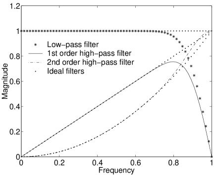
FIG. 1.: Frequency responses of the conjugate DSC filters (in the unit of $\pi/\Delta$), The maximum amplitude of the filters is normalized to the unit.

(a) t=2

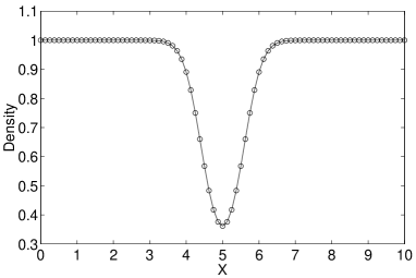
(b) t=10

(c) t=50

(d) t=100

FIG. 2.: Density profiles in horizontal cutting at four times. Solid line is the exact profile and the circle dots denote the numerical results.

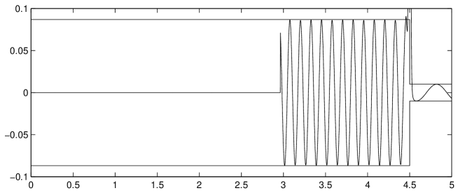
(a) $\kappa=13$, N=800

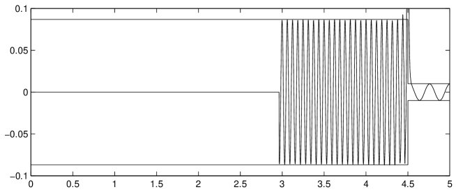
(b) $\kappa=26$, N=800

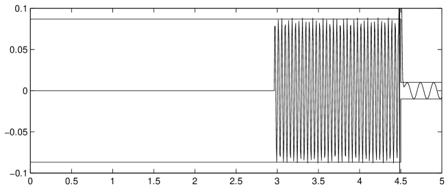
(c) $\kappa=39$, N=800, before the interpolation

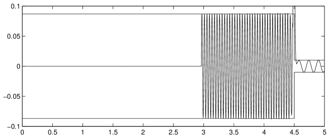
(d) $\kappa=39$, N=800, after the interpolation

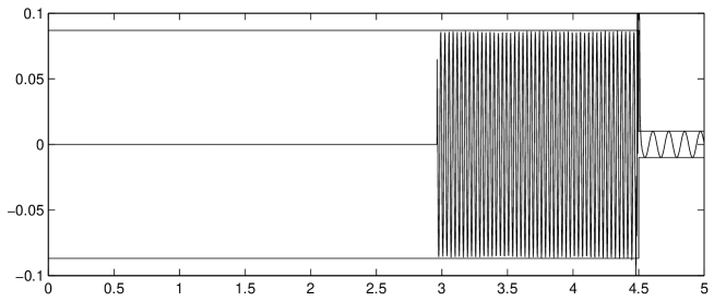
(e) $\kappa=52$, N=1600

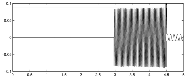
(f) $\kappa=65$, N=1600

FIG. 3.: Shock entropy wave interaction.

REFERENCES

- [1] Chi-Wang Shu, ‘Essentially non-oscillatory and weighted essentially non-oscillatory schemes for hyperbolic conservation laws’, ICASE Report, No. 97-65, (1997).
- [2] O. C. Zienkiewicz, P. Nithiarasu, R. Codina, M. Vazquez and P. Ortiz, ‘The characteristic-based-split procedure: an efficient and accurate algorithm for fluid problems’, Int. J. Numer. Meth. Fluids, 31, 359-392 (1999).
- [3] C. E. Baumann and J. T. Oden, ‘An adaptive-order discontinuous Galerkin method for the solution of the Euler equations of gas dynamics’, Int. J. Numer. Meth. Engng, 47, 61-73 (2000).
- [4] S. Lee, S. K. Lele and P. Moin, ‘Interaction of isotropic turbulence with shock waves: Effect of shock strength’, J. Fluid Mech., 340, 225 (1997).
- [5] E. Garnier, M. Mossi, P. Sagaut, P. Comet and M. Deville, ‘On the use of shock-capturing scheme for large-eddy simulation’, J. Comput. Phys. 153, 273 (2001).
- [6] B. Engquist, P. Lötstedt and B. Sjögreen, ‘Nonlinear filters for efficient shock computation’, Mathematics of Computation., 54, 509-537 (1989).
- [7] E. Garnier, P. Sagaut and M. Deville, ‘A class of explicit ENO filters with application to unsteady flows’, J. Comput. Phys., 170, 184-204 (2001).
- [8] G. W. Wei, and Y. Gu, ‘Conjugated filter approach for solving Burgers’ equation’, arXiv:math.SC/0009125, Sept. 13, (2000).
- [9] Y. Gu and G. W. Wei, ‘Conjugated filter approach for shock capturing’, submitted.
- [10] G. W. Wei, ‘Discrete singular convolution for the solution for the Fokker-Planck equations’, J. Chem. Phys., 110, 8930-8942 (1999).
- [11] G. W. Wei, ‘Wavelets generated by using discrete singular convolution kernels’, J. Phys. A, Mathematical and General, 33, 8577-8596 (2000).
- [12] G. W. Wei, ‘A new algorithm for solving some mechanical problems’, Comput. Methods Appl. Mech. Engng., 190, 2017-2030 (2001).
- [13] J. F. McKenzie and K. O. Westphal, ‘Interaction of linear waves with oblique shock waves’, Phys. Fluids, 11, 2350-2362 (1968).