Numerical Computations of Viscous, Incompressible Flow Problems Using a Two-Level Finite Element Method

Abstract

We consider two-level finite element discretization methods for the stream function formulation of the Navier-Stokes equations. The two-level method consists of solving a small nonlinear system on the coarse mesh, then solving a linear system on the fine mesh. The basic result states that the errors between the coarse and fine meshes are related superlinearly. This paper demonstrates that the two-level method can be implemented to approximate efficiently solutions to the Navier-Stokes equations. Two fluid flow calculations are considered to test problems which have a known solution and the driven cavity problem. Stream function contours are displayed showing the main features of the flow.

1 Introduction

The numerical treatment of nonlinear problems that arise in areas such as fluid mechanics often requires solving large systems of nonlinear equations. Many methods have been proposed that attempt to solve these systems efficiently; one such class of methods are two-level methods that reduce the computational time. The computational attractions of the methods are that they require the solution of only a small system of nonlinear equations on coarse mesh and one linear system of equations on fine mesh. Apparently, the two-level method was proposed first in [17, 16, 15] and used for semilinear elliptic problems. The method was implemented for the velocity-pressure formulation of the Navier-Stokes equations in [11, 12, 13] and for the stream function formulation of the Navier-Stokes equations in [8, 18, 7].

The Navier-Stokes equations may be solved using either the primitive variable or stream function formulation. Here we use the stream function formulation. The attractions of the stream function formulation are that the incompressibility constraint is automatically satisfied, the pressure is not present in the weak form, and there is only one scalar unknown to solve for. The standard weak formulation of the stream function version first appeared in 1979 in [10]. In this direction, Cayco and Nicolaides [5, 4, 3] studied a general analysis of convergence for this standard weak formulation.

The goal of this paper is to demonstrate that the two-level method can be implemented to approximate solutions for incompressible viscous flow problems with high Reynolds number.

2 Governing Equations

Consider the Navier-Stokes equations describing the flow of an incompressible fluid

$$-{\rm Re}^{-1}\bigtriangleup\vec{u}+(\vec{u}\cdot\bigtriangledown)\vec{u}+\bigtriangledown p =\vec{f} \qquad\Omega,$$ in (1)

$$\bigtriangledown\cdot\vec{u} =0 \qquad\Omega,$$ in (2)

$$\vec{u} =0 \qquad\partial\Omega,$$ on (3)

where $\vec{u}=(u_{1},u_{2})$ and $p$ denotes the unknown velocity and pressure field, respectively, in a bounded,simply connected polygonal domain $\Omega\subseteq R^{2}$. $\vec{f}$ is a given body force and Re is the Reynolds number.

The introduction of a stream function $\psi(x,y)$ defined by

$$u_{1}=-\frac{\partial\psi}{\partial y},\qquad u_{2}=\frac{\partial\psi}{\partial x},$$

means that the continuity equation (2) is satisfied identically. The pressure may then be eliminated from (1) to give

$$\mbox{Re}^{-1}\triangle^{2}\psi-\psi_{y}\triangle\psi_{x}+\psi_{x}\triangle\psi_{y} = ~{}\vec{{\rm curl}}\vec{f}\mbox{ in }\Omega,$$ (4)

$$\psi = 0\mbox{ on }\partial\Omega,$$ (5)

$$\frac{\partial\psi}{\partial\hat{n}} = 0\mbox{ on }\partial\Omega,$$ (6)

where $\hat{n}$ represents the outward unit normal to $\Omega$. In order to write (4)-(6) in a variational form, we define the Sobolev spaces

$$H^{1}(\Omega) =\{v:v\in L^{2}(\Omega),Dv\in L^{2}(\Omega)\},$$ (7)

$$H^{1}_{0}(\Omega) =\{v:v\in H^{1}(\Omega),v=0\mbox{ on }\partial\Omega\},$$ (8)

$$H^{2}(\Omega) =\{v:v\in L^{2}(\Omega),Dv\in L^{2}(\Omega),D^{2}v\in L^{2}(\Omega)\},$$ (9)

$$H^{2}_{0}(\Omega) =\{v\in H^{2}(\Omega):v=\frac{\partial v}{\partial n}=0,\mbox{ on }\partial\Omega\},$$ (10)

where $L^{2}(\Omega)$ is the space of square integrable functions on $\Omega$ and $D$ represents differentiation with respect to $x$ or $y$. For each $\phi\in H^{1}(\Omega)$, define $\vec{{\rm curl}}\;\phi=\left(\begin{array}[]{c}\phi_{y}\\ -\phi_{x}\end{array}\right)$. The standard weak form of equations (4)-(6) is:

$$\begin{split}\mbox{Find }\psi\in H_{0}^{2}(\Omega)\mbox{ such that, for all }\phi\in H_{0}^{2}(\Omega),\\ a(\psi,\phi)+b(\psi;\psi,\phi)=l(\phi),\end{split}$$ (11)

where

$$\begin{split}a(\psi,\phi)&=Re^{-1}\int_{\Omega}\bigtriangleup\psi\cdot\bigtriangleup\phi~{}d\Omega,\\ b(\xi;\psi,\phi)&=\int_{\Omega}\bigtriangleup\xi(\psi_{y}\phi_{x}-\psi_{x}\phi_{y})~{}d\Omega,\\ l(\phi)&=(\vec{f},\vec{\mbox{curl}\phi})=\int_{\Omega}\vec{f}\cdot\vec{\mbox{curl}}\phi~{}d\Omega.\end{split}$$

3 Finite Element Discretization

For the standard finite element discretization of (11) we choose subspace $X^{H}\subset H^{2}_{0}(\Omega)$. We then

$$\begin{split}\mbox{seek }\psi^{H}\in X^{H}\mbox{ such that, for all }\phi^{H}\in X^{H},\\ a(\psi^{H},\phi^{H})+b(\psi^{H};\psi^{H},\phi^{H})=l(\phi^{H}).\end{split}$$ (12)

One can prove existence and uniqueness for the solution of the discrete problem (12) ; see [5] for low Reynolds numbers and see [8, 7] for high Reynolds numbers.

Once the finite element spaces are prescribed, the discrete problem (12) reduces to solving a system of nonlinear algebraic equations which has a Jacobian which is large, sparse and bounded. Various iterative methods can be used to solve the nonlinear problem (12). For example, a standard approach is to use Newton’s method to linearize (12) for a fixed mesh of size $h$. Since only one fixed mesh spacing is used, we will refer to this approach as a one-level approach. In the next section we will describe a two-level method for solving the discrete problem (12).

4 Two-level Method

We consider the approximate solution of (4) by a two-level, finite-element procedure. Let $X^{h},X^{H}\subset H^{2}_{0}(\Omega)$ denote two conforming finite-element meshes with $H\gg h$. The method we consider computes an approximate solution $\psi^{h}$ in the finite-element space $X^{h}$ by solving one linear system for the degrees of freedom on $X^{h}$. This particular linear problem requires the construction of a finite-element space $X^{H}$ upon a very coarse mesh of width ’$H\gg h$’, and then the solution of a much smaller system of nonlinear equations for an approximation in $X^{H}$. The solution procedure is then given in Algorithm 1.

Algorithm 1 The Two-Level Algorithm

Step 1. Solve the nonlinear system on coarse mesh for $\psi^{H}\in X^{H}$:

$$a\left(\psi^{H},\phi^{H}\right)+b\left(\psi^{H},\psi^{H},\phi^{H}\right)=\left(\vec{f},\vec{{\rm curl}}\;\phi^{H}\right),\hskip 19.91692pt\mbox{ for all }~{}\phi^{H}\in X^{H}.$$ (13)

Step 2. Solve the linear system on fine mesh for $\psi^{h}\in X^{h}$:

$$a\left(\psi^{h},\phi^{h}\right)+b\left(\psi^{H},\psi^{h},\phi^{h}\right)=\left(\vec{f},\vec{{\rm curl}}\;\phi^{h}\right),\hskip 19.91692pt\mbox{ for all }~{}\phi^{h}\in X^{h}.$$ (14)

The inclusion $X^{H}\subset H^{2}_{0}(\Omega)$ requires the use of finite-element functions that are continuously differentiable over $\Omega$. We shall give some examples of finite-element spaces for the stream function formulation  (see  [6, 3]). We will impose boundary conditions by setting all the degrees of freedom at the boundary nodes to be zero and the normal derivative equal to zero at all vertices and nodes on the boundary.

Argyis Triangle. The functions are quintic polynomials within each triangle and the 21 degrees of freedom are chosen to be the function value, the first and second derivatives at the vertices, and the normal derivative at the midsides.

Clough-Tocher Triangle. Here we subdivide each triangle into three triangles by joining the vertices to the centroid. In each of the smaller triangles, the functions are cubic polynomials. There are then 30 degrees of freedom needed to determine the three different cubic polynomials associated with the three triangles. Eighteen of these are used to ensure that, within the big triangle, the functions are continuously differentiable. The remaining 12 degrees of freedom are chosen to be the function values and the first derivatives at the vertices and the normal derivative at the midsides.

Bogner-Fox-Schmit Rectangle. The functions are bicubic polynomials within each rectangle. The degrees of freedom are chosen to be the function value, the first derivatives, and the mixed second derivative at the vertices. We set the function and the normal derivative values equal to zero at all vertices on the boundary.

Bicubic Spline Rectangle. The functions are the product of cubic splines. These functions are bicubic polynomials within each rectangle, are twice continuously differentiable over $\Omega$, and their degrees of freedom are the function values at the nodes (plus some additional ones on the boundary).

The question which automatically arises is how to choose $X^{H}$ and $X^{h}$ so that we obtain optimal accuracy. This question was addressed from a theoretical standpoint in [8] and the results are summarized below. In [8], it was proven that the algorithm produces an approximate solution which satisfies the error bound

$$\left|\psi-\psi^{h}\right|_{2}\leq C\left\{\inf_{w^{h}\in X^{h}}\left|\psi-w^{h}\right|_{2}+\left|\ln h\right|^{1/2}\cdot\left|\psi-\psi^{H}\right|_{1}\right\}.$$ (15)

As an example, consider the case of the Clough-Tocher triangle. For this element we have the following inequalities:

$$\left|\psi-\psi^{h}\right|_{j}\leq Ch^{4-j}\hskip 19.91692pt(j=0,1,2),$$

$$\left|\psi-\psi^{H}\right|_{j}\leq CH^{4-j}\hskip 19.91692pt(j=0,1,2).$$

Thus, if we seek an approximate solution $\psi^{h}$ with the same asymptotic accuracy as $\psi^{h}$ in $|\cdot|_{2}$, the above error bound shows that the superlinear scaling, between coarse and fine meshes,

$$h=O\left(H^{3/2}|\ln H|^{1/4}\right),$$ (16)

suffices. Analogous scalings between coarse and fine meshes can be calculated from (15) by balancing error terms on the right-hand side of (15) in the same way. For each of the elements described above, we give, in Table 1, the scaling between coarse and fine meshes.

Element	$\mid\psi-\psi^{H}\mid_{2}$	$\mid\psi-\psi^{H}\mid_{1}$	Scaling
Argyris triangle	$H^{4}$	$H^{5}$	$h\mid\ln h\mid^{-1/4}=O(H^{5/2})$
Clough-Tocher triangle	$H^{2}$	$H^{3}$	$h\mid\ln h\mid^{-1/4}=O(H^{3/2})$
Bogner-Fox-Schmit rectangle	$H^{2}$	$H^{3}$	$h\mid\ln h\mid^{-1/4}=O(H^{3/2})$
Bicubic spline rectangle	$H^{2}$	$H^{3}$	$h\mid\ln h\mid^{-1/4}=O(H^{3/2})$

Table 1: Scaling between coarse and fine meshes

5 Numerical Examples

In this section we describe some numerical results obtained by implementing the two-level algorithm for which we have an exact solution and the second is the well-known driven cavity problem. We chose the later problem because there are numerous results in the literature with which to compare.

For both examples, the region $\Omega$ is the unit square $\{0<x<1,\;0<y<1\}$ and for the finite element discretization we use the Bogner-Fox-Schmit elements. In order to compare the efficiency of the proposed method all linear and nonlinear systems were solved in the same way. All nonlinear problems were solved by Newton’s method until the norm of the difference in successive iterates and the norm of residual were within a fixed tolerance. In each Newton’s iteration, we need to solve a linear system. The resulting linear system is non-symmetric whose symmetric part is positive definite. Moreover, the resulting matrix is sparse matrix. We choose the Bi-Conjugate Gradient Stabilized method (BICGSTAB) which requires two matrix-vector products and four inner products in each iteration. BICGSTAB is given and discussed in [2]. When solving the linearized problem with a mesh spacing $h$ we need the solution $u^{H}$ generated on a mesh with spacing $H$. To do this we interpolate the solution $u^{H}$ onto the grid with spacing $h$.

Example 1

We consider as a test example the 2D Navier-Stokes equations (1)- (3) on the unit square $\Omega=(0,1)^{2}$ where we define the right hand side by $f:=-Re^{-1}\bigtriangleup\vec{u}+(\vec{u}\cdot{\bf\bigtriangledown})\vec{u}+\bigtriangledown p$ with the following prescribed exact solution

$$u = \left(\begin{array}[]{c}\psi_{y}\\ -\psi_{x}\end{array}\right)\hskip 19.91692pt\mbox{with }\;\psi(x,y)=x^{2}(x-1)^{2}y^{2}(y-1)^{2},$$

$$p = x^{3}+y^{3}-0.5.$$

For this test problem, all requirements of the theory concerning the geometry of the domain and the smoothness of the data are satisfied. Moreover, the stream function $\psi(x,y)$ satisfies the boundary conditions of the stream function equation of the Navier-Stokes equations.

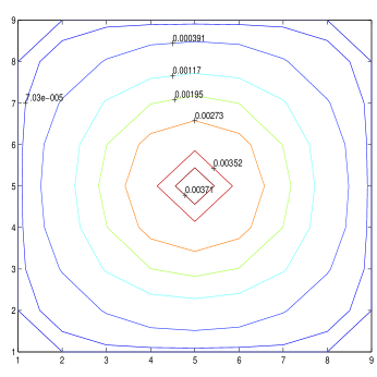
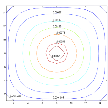
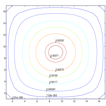
Fig. 1: Left-side: streamlines for $h=\frac{1}{8},\frac{1}{14},\frac{1}{16}$ with Re = 10 using the one-level method. Right-side: streamlines for $(H,h)=\left(\frac{1}{4},\frac{1}{8}\right),\left(\frac{1}{7},\frac{1}{14}\right),\left(\frac{1}{8},\frac{1}{16}\right)$ with Re = 10 using the two-level method.

Our goal in this test is to validate the code and the properties and merits of the two-level method as compared with the one-level method. In all numerical calculations in this example we have used the Bogner-Fox-Schmit elements with $\mbox{Re}=10$ and $\mbox{tol}=10^{-3}$. We pick three values of $h$. They are $\frac{1}{8},\frac{1}{14}$ and $\frac{1}{16}$. The cpu-time, number of Newton’s iterations, number of Bicgstab iterations, the $L^{2}$-error and $H^{2}$-error of the stream function $\psi$ for the one-level method for different values of $h$ are tabulated in Table LABEL:table2. Table LABEL:table3 shows cup-time, number of Newton’s iterations and the number of Bicgstab’s iterations for each linear solver for the two-level method. Figure 1 shows, for fixed $\mbox{Re}=10$ using the one-level and two-level method, the streamlines for $h=\frac{1}{8};\frac{1}{14};\frac{1}{16}$.

Remarks

1. From Tables LABEL:table2 and LABEL:table3, the cpu-time for the two-level method is much smaller than the corresponding cpu-time for the one-level method. For $h=\frac{1}{8},\frac{1}{14}$, we save about 57%. For example, in $h=\frac{1}{16}$ we save about 73%. For example, in $h=\frac{1}{16}$ we need to solve a nonlinear system of 1156 equations which requires solving three linear systems of equations of order 1156. The corresponding two-level method requires solving a nonlinear system of 324 equations and a linear system of 1156 equations. We anticipate the savings to increase as the mesh is further refined.

2. From Figures 1 , both columns are exactly the same, which means that the two-level method produces a solution with the same quality as the one-level method.

3. From Tables LABEL:table2 and LABEL:table3, both $H^{1}$-error and $H^{2}$-error are of the same order, which means that the velocity field is of the same error and quality in both methods since $u=\psi_{y}$ and $v=-\psi_{x}$.

Table 2: One level method. where ni = number of Newton’s iteration, nb = number of Bicgstab iterations

$h$	cpu time	ni	nb	$\parallel\psi-\psi^{h}\parallel_{0,h}$	$\parallel\psi-\psi^{h}\parallel_{1,h}$	$\parallel\psi-\psi^{h}\parallel_{2,h}$
$\frac{1}{8}$	69.74	3	26,30,24	3.94$\times 10^{-5}$	4.23$\times 10^{-2}$	1.41$\times 10^{-1}$
$\frac{1}{14}$	294.35	3	50,56,55	2.41$\times 10^{-5}$	1.74$\times 10^{-2}$	8.87$\times 10^{-2}$
$\frac{1}{16}$	992.23	3	63,75,67	3.55$\times 10^{-5}$	1.41$\times 10^{-2}$	8.08$\times 10^{-2}$

Table 3: Two level method. where noc = number of Bicgstab iterations in coarse, nof = number of Bicgstab iterations in fine

$H,h$	cpu time	noc	nof	$\parallel\psi-\psi^{h}\parallel_{0,h}$	$\parallel\psi-\psi^{h}\parallel_{1,h}$	$\parallel\psi-\psi^{h}\parallel_{2,h}$
$\frac{1}{4},\frac{1}{8}$	29.91	10,18,15	50	1.40$\times 10^{-3}$	4.09$\times 10^{-2}$	1.42$\times 10^{-1}$
$\frac{1}{7},\frac{1}{14}$	128.28	22,24,21	118	2.31$\times 10^{-4}$	1.73$\times 10^{-2}$	8.70$\times 10^{-2}$
$\frac{1}{8},\frac{1}{16}$	267.33	26,30,24	169	1.70$\times 10^{-4}$	1.41$\times 10^{-2}$	7.94$\times 10^{-2}$

Example 2

In this example, we consider the problem which was described in Example 1. The exact solution is very smooth and does not depend on the Reynolds number. The point of these tests is to increase the Reynolds number with $h$ fixed and test the robustness of the method. Our goal in this test is to determine the validation of the code and the norm behavior when Re is varying. Schieweck [14] tested his code with this problem. He used two nonconforming finite element approximations of upwind type for the velocity-pressure formulation.

The numerical computations of this example were obtained using a Sun Ultra 2 with 2 200 Mhz ultrasparc processor running Solaris 2.5.1. In all numerical calculations, we used the Bogner-Fox-Schmit rectangles. The streamlines for Re = 100, 1000 and 2000 were obtained with $17\times 17$ grid points on the coarse mesh and $33\times 33$ grid on the fine mesh. Hence, a mesh of 256 elements and a mesh of 1024 elements were used in this test for the case of Bgner-Fox-Schmit rectangles.

Table LABEL:table4 represents the $L^{2}$-error, $H^{1}$-error and $H^{2}$-error. The streamlines are plotted in Figure 2 for Re = 100, 1000, 2000. Figure  2 shows that an increase in the Reynolds number will affect the streamlines and increase the number of corner contours.
Example 3
Cavity flows have been a subject of study for some time. These flows have been widely used as test cases for validating incompressible fluid dynamics algorithm. Corner singularities for two-dimensional fluid flows are very important since most examples of physical interest have corners. For example, singularities of most elliptic problems develop when the boundary contour is not smooth. In this example, we consider the driven flow in a rectangular cavity when the top surface moves with a constant velocity along its length. The upper corners where the moving surface meets the stationary walls are singular points of the flow at which the horizontal velocity is multi-valued. The lower corners are also weakly singular points.

We consider a domain $\Omega=[0,1]\times[0,1]$ with no-slip boundary conditions, i.e., $u=v=0$ in all boundaries except $y=1$, where $u=1$. This problem has been studied and addressed by many researchers including Ghia, Ghia, Shin [9], and J.E. Akin [1]. The numerical computation of this example was obtained using a Sun Ultra 2 with 2 200 MHz ultrasparc processor running Solaris 2.5.1. Bogner-Fox-Schmit elements are used with $17\times 17$ grid points on the coarse mesh and $33\times 33$ grid points on the fine mesh. The streamlines for Re = 1, 10, 50, 100 are plotted in Figure 3. Figure 4 shows the $u$-velocity lines through the vertical line $x=0.5$ and $v$-velocity lines through the horizontal line $y=0.5$.

Table 4: Two level for test problem. where noc = number of Bicgstab iterations in coarse , nof = number of Bicgstab iteration in fine

$Re$	(H,h)	noc	nof	$\parallel\psi-\psi^{h}\parallel_{0,h}$	$\parallel\psi-\psi^{h}\parallel_{1,h}$	$\parallel\psi-\psi^{h}\parallel_{2,h}$
10	$(\frac{1}{16},\frac{1}{32})$	61,66,43	576	4.21$\times 10^{-5}$	4.84$\times 10^{-3}$	5.27$\times 10^{-2}$
50	$(\frac{1}{16},\frac{1}{32})$	54,83,173,	1676	1.11$\times 10^{-4}$	4.82$\times 10^{-3}$	5.19$\times 10^{-2}$
		292,82
100	$(\frac{1}{16},\frac{1}{32})$	53,254,421,	4356	4.44$\times 10^{-4}$	5.00$\times 10^{-3}$	5.11$\times 10^{-2}$
		668,1287
200	$(\frac{1}{16},\frac{1}{32})$	53,254,421,	4356	3.06$\times 10^{-4}$	4.52$\times 10^{-3}$	5.07$\times 10^{-2}$
		668,1287,454
1000	$(\frac{1}{16},\frac{1}{32})$	53,254,421,	4356	9.62$\times 10^{-4}$	1.08 $\times 10^{-2}$	1.83 $\times 10^{-1}$
		668,1287,1156
2000	$(\frac{1}{16},\frac{1}{32})$	53,254,421,	4356	1.93 $\times 10^{-3}$	2.59 $\times 10^{-2}$	4.93 $\times 10^{-1}$
		668,1287,1156,
		1156,1156

   

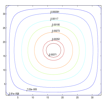
(a) Exact

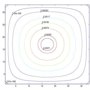
(b) Re=100

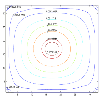
(c) Re=1000

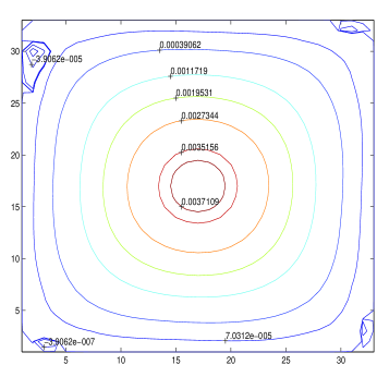
(d) Re=2000

Fig. 2: Streamlines for $H=\frac{1}{16},h=\frac{1}{32}$ using Bogner-Fox-Schmit element.

   

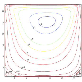
(a) Re=1

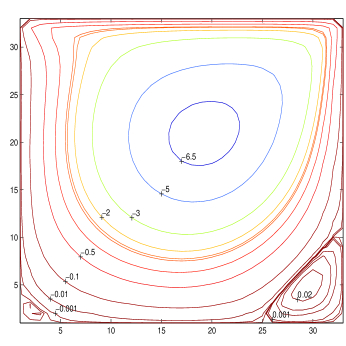
(b) Re=10

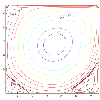
(c) Re=50

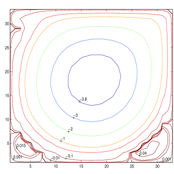
(d) Re=100

Fig. 3: Cavity Problem : Streamlines for $H=\frac{1}{16},h=\frac{1}{32}$ with different values of Re numbers using two level method

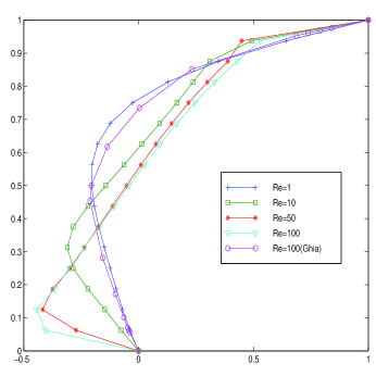
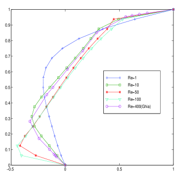
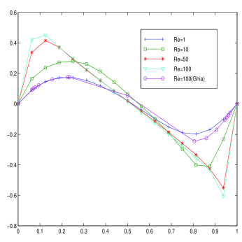
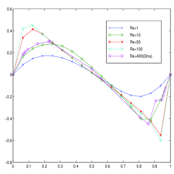
Fig. 4: Cavity Problem :(above)$u$-velocity lines through the vertical line $x=0.5$ for different Reynolds number and Ghia lines for Re=400, (below) $v$-velocity lines through the horizontal line $y=0.5$ for different Reynolds number and Ghia lines for Re=400. (courtesy U. Ghia [9])

References

- [1] J. Akin. finite element for analysis and design. Academic Press, San Diego, 1994.
- [2] R. Barrett, M. Berry T. Chan J. Demmel J. Donator J. Doncarra V. Eijkhout R. Pozo C. Romine and H. Van dev Vorst, Templates: for the solution of linear systems: building blocks for iterative methods. e-mail : templates@cs.utk.edu.
- [3] M. Cayco. Finite Element Methods for the Stream Function Formulation of the Navier-Stokes Equations. PhD thesis, CMU, Pittsburgh, PA., 1985.
- [4] M. Cayco and R.A. Nicolaides. Analysis of nonconforming stream function and pressure finite element spaces of the Navier-Stokes equations. Comp. and Math. Appl., (8): 745–760, 1989.
- [5] M. Cayco and R.A. Nicolaides. Finite element technique for optimal pressure recovery from stream function formulation of viscous flows. Math. Comp., (56): 371–377, 1986.
- [6] Ph. G. Ciarlet, the finite element method for elliptic problems, North Holland, Amsterdam, 1978
- [7] F. Fairag. A Two-Level Discretization Method For The Streamfunction Form of The Navier-Stokes Equations. PhD thesis, University of Pittsburgh, Pittsburgh, PA., 1998.
- [8] F. Fairag. Two-level finite element method for the stream function formulation of the Navier-Stokes equations. Computers Math. Applic., 36(2): 117–127, 1998.
- [9] K.N. Ghia U. Ghia and C.T. Shin. High Re solutions for incompressible flow using the Navier-Stokes equations and a multigrid method. J. Comput. Phys., 48: 387–411, 1982.
- [10] V. Girault and P. A. Raviart. Finite Element Approximation of the Navier-Stokes Equations, volume 749. Springer, Berlin, 1979.
- [11] W. Layton. A two-level discretization method for the Navier-Stokes equations. Computers Math. Applic., 26:33–38, 1993.
- [12] W. Layton and W. Lenferink. Two-level Picard-defect corrections for the Navier-Stokes equations at high Reynolds number. Applied Math. and Computing, 1995.
- [13] W. Layton and W. Lenferink, A multilevel mesh independence principle for the Navier-Stokes equations, SIAM J. N. A. (1996)
- [14] F. Schieweck. On the order of two noncomforming finite element approximations of upwind type for the Navier-Stokes equations. To be published in: Proceeding of the international Workshop on Numerical Methods for the Navier-Stokes Equations, Heidelberg, October 25-28, 1993, to appear in the series Notes on Numerical Fluid Mechanics, Vieweg-Verlag.
- [15] J. Xu. A novel two-grid method for semilinear elliptic equations. SIAM J. Sci. Comput. 15(1): 231–237, 1994.
- [16] J. Xu, Some Two-Grid Finite Element Methods, chapter 157, pages 79–87. Number 157 in In Domain Decomposition Methods in Science and Engineering. Amer. Math. Soc., Providence, RI, 1994.
- [17] J. Xu. Some two-grid finite element methods. Technical report, P. S.U., 1992.
- [18] X. Ye. Two-level discretizations of the stream function form of the Navier-Stokes equations. University of Pittsburgh.