The Rank and Minimal Border Strip
Decompositions of a Skew Partition
Richard P. Stanley
Department of Mathematics
Massachusetts Institute of Technology
Cambridge, MA 02139
e-mail: rstan@math.mit.edu
version of 13 September 2001

1 Introduction.

Let $\lambda=(\lambda_{1},\lambda_{2},\dots)$ be a partition of the integer $n$, i.e., $\lambda_{1}\geq\lambda_{2}\geq\cdots\geq 0$ and $\sum\lambda_{i}=n$. The (Durfee or Frobenius) rank of $\lambda$, denoted rank$(\lambda)$, is the length of the main diagonal of the diagram of $\lambda$, or equivalently, the largest integer $i$ for which $\lambda_{i}\geq i$ [11, p. 289]. We will assume familiarity with the notation and terminology involving partitions and symmetric functions found in [7] and [11]. Nazarov and Tarasov [9, §1], in connection with tensor products of Yangian modules $Y(\mathfrak{gl}_{n})$, defined a generalization of rank to skew partitions (or skew diagrams) $\lambda/\mu$. There are several simple equivalent definitions of rank$(\lambda/\mu)$ which we summarize in Proposition 3. In particular, rank$(\lambda/\mu)$ is the least integer $r$ such that $\lambda/\mu$ is a disjoint union of $r$ border strips (also called ribbons or rim hooks). In Section 4 we consider the structure of the decompositions of $\lambda/\mu$ into this minimal number $r$ of border strips. For instance, we show that the number of ways to write $\lambda/\mu$ as a disjoint union of $r$ border strips is a perfect square. A consequence of our results will be that if $\chi^{\lambda/\mu}$ is the skew character of the symmetric group $\mathfrak{S}_{n}$ indexed by $\lambda/\mu$ and if $w$ is a permutation in $\mathfrak{S}_{n}$ with $\mathrm{rank}(\lambda/\mu)$ cycles (in its disjoint cycle decomposition) for which exactly $m_{i}$ cycles have length $i$, then $\chi^{\lambda/\mu}(w)$ is divisible by $m_{1}(w)!m_{2}(w)!\cdots$.

In addition to the various characterizations of rank$(\lambda/\mu)$ given by Proposition 3 we have a further possible characterization which we have been unable to prove or disprove. Namely, let $s_{\lambda/\mu}(1^{t})$ denote the skew Schur function $s_{\lambda/\mu}$ evaluated at $x_{1}=\cdots=x_{t}=1$, $x_{i}=0$ for $i>t$. For fixed $\lambda/\mu$, $s_{\lambda/\mu}(1^{t})$ is a polynomial in $t$. Let zrank$(\lambda/\mu)$ denote the exponent of the largest power of $t$ dividing $s_{\lambda/\mu}(1^{t})$ (as a polynomial in $t$). It is easy to see (Proposition 3) that zrank$(\lambda/\mu)\geq\mathrm{rank}(\lambda/\mu)$, and we ask whether equality always holds. We know of two main cases where the answer is affirmative: (1) when $\lambda/\mu$ is an ordinary partition (i.e., $\mu=\emptyset$), a trivial consequence of known results on Schur functions (Theorem 3(a)), and (2) when every row of the Jacobi-Trudi matrix for $\lambda/\mu$ which contains an entry equal to 0 also contains an entry equal to 1 (Theorem 3(b)).

2 Characterizations of Frobenius rank.

Let $\lambda/\mu$ be a skew shape, which we identify with its Young diagram $\{(i,j)\,:\,\mu_{i}<j\leq\lambda_{i}\}$. We regard the points $(i,j)$ of the Young diagram as squares. An outside top corner of $\lambda/\mu$ is a square $(i,j)\in\lambda/\mu$ such that $(i-1,j),(i,j-1)\not\in\lambda/\mu$. An outside diagonal of $\lambda/\mu$ consists of all squares $(i+p,j+p)\in\lambda/\mu$ for which $(i,j)$ is a fixed outside top corner. Similarly an inside top corner of $\lambda/\mu$ is a square $(i,j)\in\lambda/\mu$ such that $(i-1,j),(i,j-1)\in\lambda/\mu$ but $(i-1,j-1)\not\in\lambda/\mu$. An inside diagonal of $\lambda/\mu$ consists of all squares $(i+p,j+p)\in\lambda/\mu$ for which $(i,j)$ is a fixed inside top corner. If $\mu=\emptyset$, then $\lambda/\mu$ has one outside diagonal (the main diagonal) and no inside diagonals. Figure 1 shows the skew shape $8874/411$, with outside diagonal squares marked by + and inside diagonal squares by $-$.

Figure 1: Outside and inside diagonals of the skew shape $8874/411$

Let $d^{+}(\lambda/\mu)$ (respectively, $d^{-}(\lambda/\mu)$) denote the total number of outside diagonal squares (respectively, inside diagonal squares) of $\lambda/\mu$. Following Nazarov and Tazarov [9, §1], we define the (Durfee or Frobenius) rank of $\lambda/\mu$, denoted $\mathrm{rank}(\lambda/\mu)$, to be $d^{+}(\lambda/\mu)-d^{-}(\lambda/\mu)$. Clearly when $\mu=\emptyset$ this reduces to the usual definition of $\mathrm{rank}(\lambda)$ mentioned in the introduction. We see, for instance, from Figure 1 that $\mathrm{rank}(8874/411)=4$.

We wish to give several equivalent definitions of $\mathrm{rank}(\lambda/\mu)$. First we discuss the necessary background. A skew shape $\lambda/\mu$ is connected if the interior of the Young diagram of $\lambda/\mu$, regarded as a union of solid squares, is a connected (open) set. A border strip [11, p. 345] is a connected skew shape with no $2\times 2$ square. (The empty diagram $\emptyset$ is not a border strip.) A border strip is uniquely determined, up to translation, by its row lengths; there are exactly $2^{n-1}$ border strips with $n$ squares (up to translation). We say that a border strip $B\subseteq\lambda/\mu$ is a border strip of $\lambda/\mu$ if $\lambda/\mu-B$ is a skew shape $\nu/\mu$ (so $B=\lambda/\nu$). Equivalently, we say that $B$ can be removed from $\lambda/\mu$. A border strip $B$ of $\lambda/\mu$ is determined by its lower left-hand square init$(B)$ and upper right-hand square fin$(B)$. A border strip decomposition [11, p. 470] of $\lambda/\mu$ is a partitioning of the squares of $\lambda/\mu$ into (pairwise disjoint) border strips. Let $N=|\lambda/\mu|:=\sum\lambda_{i}-\sum\mu_{i}$ and $\sigma=(\sigma_{1},\dots,\sigma_{\ell})\vdash N$, where $\sigma_{\ell}>0$. We say that a border strip decomposition $D$ has type $\sigma\vdash N$ if the sizes (number of squares) of the border strips appearing in $D$ are $\sigma_{1},\dots,\sigma_{\ell}$. A border strip decomposition of $\lambda/\mu$ is minimal if the number of border strips is minimized, i.e., there does not exist a border strip decomposition with fewer border strips. Figure 2 shows a minimal border strip decomposition of the skew shape $8874/411$.

Figure 2: A minimal border strip decomposition of the skew shape $8874/411$

A concept closely related to border strip decompositions is that of border strip tableaux [11, p. 346]. Let $\lambda/\mu\vdash N$. Let $\alpha=(\alpha_{1},\alpha_{2},\dots,\alpha_{m})$ be a composition of $N$, i.e., $\alpha_{i}\in\mathbb{P}=\{1,2,\dots\}$ and $\sum\alpha_{i}=N$. A border strip tableau of (shape) $\lambda/\mu$ and type $\alpha$ is a sequence

$$\mu=\lambda^{0}\subset\lambda^{1}\subset\cdots\subset\lambda^{r}=\lambda$$ (1)

such that $\lambda^{i}/\lambda^{i-1}$ is a border strip of size $\alpha_{i}$. (Note that the type of a border strip decomposition is a partition but of a border strip tableau is a composition.) Every border strip tableau $T$ of shape $\lambda/\mu$ defines a border strip decomposition $D$ of $\lambda/\mu$, viz., the border strips $\lambda^{i}/\lambda^{i-1}\neq\emptyset$ of $T$ are just the border strips of $D$. We say that $D$ corresponds to $T$ and conversely that $T$ corresponds to $D$. Of course given $T$, the corresponding $D$ is unique, but not conversely. If $T$ corresponds to a minimal border strip decomposition $D$, then we call $T$ a minimal border strip tableau.

Now suppose that $\ell(\lambda)\leq n$, where $\ell(\lambda)$ denotes the number of (nonzero) parts of $\lambda$. Recall that the Jacobi-Trudi identity for the skew Schur function $s_{\lambda/\mu}$ [11, Thm. 7.16.1] asserts that

$$s_{\lambda/\mu}=\det\left(h_{\lambda_{i}-\mu_{j}-i+j}\right)_{i,j=1}^{n},$$

where $h_{k}$ denotes the complete homogeneous symmetric function of degree $k$, with the convention $h_{0}=1$ and $h_{k}=0$ for $k<0$. Denote the matrix $\left(h_{\lambda_{i}-\mu_{j}-i+j}\right)$ appearing in the Jacobi-Trudi identity by JT_λ/μ, called the Jacobi-Trudi matrix of the skew shape $\lambda/\mu$. Let jrank$(\lambda/\mu)$ denote the number of rows of JT_λ/μ that don’t contain a 1. Note that JT_λ/μ implicitly depends on $n$, but jrank$(\lambda/\mu)$ does not depend on the choice of $n$.

Our final piece of background material concerns the (Comét) code of a shape $\lambda$ [11, Exer. 7.59], generalized to skew shapes $\lambda/\mu$. Let $\lambda/\mu$ be a skew shape, with its left-hand edge and upper edge extended to infinity, as shown in Figure 3 for $\lambda/\mu=8874/411$. Put a 0 next to each vertical edge and a 1 next to each horizontal edge of the “lower envelope” and “upper envelope” of $\lambda/\mu$ (whose definition should be clear from Figure 3). If we read these numbers as we move north and east along the lower envelope we obtain an infinite binary sequence $C_{\lambda/\mu}=\cdots c_{-2}c_{-1}c_{0}c_{1}c_{2}\cdots$ beginning with infinitely many 0’s and ending with infinitely many 1’s. Similarly if read these numbers as we move north and east along the upper envelope we obtain another such binary sequence $D_{\lambda/\mu}=\cdots d_{-2}d_{-1}d_{0}d_{1}d_{2}\cdots$. The indexing of the terms of $C_{\lambda/\mu}$ and $D_{\lambda/\mu}$ is arbitrary (it doesn’t affect the sequences themselves), but we require them to “line up” in the sense that common steps in the two envelopes should have common indices. We call the resulting two-line array

$$\mathrm{code}(\lambda/\mu)=\begin{array}[]{cccccccc}\cdots&c_{-2}&c_{-1}&c_{0}&c_{1}&c_{2}&\cdots\\ \cdots&d_{-2}&d_{-1}&d_{0}&d_{1}&d_{2}&\cdots\end{array},$$ (2)

the (Comét) code of $\lambda/\mu$ (also known as the partition sequence of $\lambda$ [1][2]). If we omit the infinitely many initial columns ${0\atop 0}$ and final columns ${1\atop 1}$ from $\mathrm{code}(\lambda/\mu)$, then we call the resulting array the reduced code of $\lambda/\mu$, denoted $\overline{\mathrm{code}}(\lambda/\mu)$. Thus for instance from Figure 3 we see that

$$\overline{\mathrm{code}}(8874/411)=\begin{array}[]{cccccccccccc}1&1&1&1&0&1&1&1&0&1&0&0\\ 0&1&0&0&1&1&1&0&1&1&1&1\end{array}.$$

A two-line array (2) with infinitely many initial columns ${0\atop 0}$ and final columns ${1\atop 1}$ is the code of some $\lambda/\mu$ if and only if for all $i$,

$$\#\{j\leq i\,:\,(c_{j},d_{j})=(1,0)\}\geq\#\{j\leq i\,:\,(c_{j},d_{j})=(0,1)\},$$ (3)

and if

$$\#\{j\in\mathbb{Z}\,:\,(c_{j},d_{j})=(1,0)\}=\#\{j\in\mathbb{Z}\,:\,(c_{j},d_{j})=(0,1)\}.$$ (4)

If $\mu=\emptyset$ then the second row of code$(\lambda/\mu)$ is redundant, so we define code$(\lambda)$ to be the first row of code$(\lambda/\mu)$. If $\mathrm{code}(\lambda/\mu)$ is given by (2) then we write $s(c_{i})$ (respectively, $s(d_{i})$) for the (unique) square of $\lambda/\mu$ that contains the edge of the lower envelope (respectively, upper envelope) of $\lambda/\mu$ corresponding to $c_{i}$ (respectively, $d_{i}$). The following fundamental property of code$(\lambda/\mu)$ appears e.g. in [11, Exer. 7.59(b)] for ordinary shapes and carries over directly to skew shapes.

Figure 3: Constructing the code of $8874/411$

2.1 Proposition.   Let $\mathrm{code}(\lambda/\mu)$ be given by (2). Then removing a border strip of size $p$ from $\lambda/\mu$ is equivalent to choosing $i$ with $c_{i}=1$ and $c_{i+p}=0$, and then replacing $c_{i}$ with 0 and $c_{i+p}$ with 1, provided that (3) continues to hold. Specifically, such a pair $(i,i+p)$ corresponds to the border strip $B$ of size $p$ defined by

$$\mathrm{init}(B)=s(c_{i}),\quad\mathrm{fin}(B)=s(c_{i+p}).$$

Moreover, code$(\lambda/\mu-B)$ is obtained from code$(\lambda/\mu)$ by setting $c_{i}=0$ and $c_{i+p}=1$.

We can now state several characterizations of $\mathrm{rank}(\lambda/\mu)$.

2.2 Proposition.   For any skew shape $\lambda/\mu$, the following numbers are equal.

1. rank$(\lambda/\mu)$

2. the number of border strips in a minimal border strip decomposition of $\lambda/\mu$

3. jrank$(\lambda/\mu)$

4. the number of columns of $\mathrm{code}(\lambda/\mu)$ equal to ${0\atop 1}$ (or to ${1\atop 0}$)

Proof. By equations (3) and (4) there exists a bijection

$$\vartheta:\{i\,:\,(c_{i},d_{i})=(1,0)\}\rightarrow\{i\,:\,(c_{i},d_{i})=(0,1)\}$$

such that $\vartheta(i)>i$ for all $i$ in the domain of $\vartheta$. By Proposition 3, as we successively remove border strips from $\lambda/\mu$ the bottom line $\cdots d_{-1}d_{0}d_{1}\cdots$ of code$(\lambda/\mu)$ remains the same, while the top line $\cdots c_{-1}c_{0}c_{1}\cdots$ interchanges a 0 and 1. We will exhaust all of $\lambda/\mu$ when the top line becomes equal to the bottom. Hence the number of border strips appearing in a border strip decomposition of $\lambda/\mu$ is at least the number of columns ${0\atop 1}$ of code$(\lambda/\mu)$. On the other hand, we can achieve exactly this number by interchanging $c_{i}$ with $c_{\vartheta(i)}$ for all $i$ such that $(c_{i},d_{i})=(0,1)$. It follows that (b) and (d) are equal.

Let $B$ be the (unique) largest border strip of $\lambda/\mu$ such that init$(B)$ is the bottom square of the leftmost column of $\lambda/\mu$. $B$ will intersect each diagonal (running from upper-left to lower-right) of its connected component $\sigma$ of $\lambda/\mu$ exactly once. The number of outside diagonals of $\sigma$ is one more than the number of inside diagonals. Hence rank$(\lambda/\mu)=\mathrm{rank}(\lambda/\mu-B)+1$. Continuing to remove the largest border strip results in a minimal border strip decomposition of $\lambda/\mu$. (Minimality is an easy consequence of Proposition 3.) Since each border strip removal reduces the rank by one, it follows that (a) and (b) are equal.

Finally consider the Jacobi-Trudi matrix JT_λ/μ. We prove by induction on the number of rows of JT_λ/μ that (b) and (c) are equal. The assertion is clear when JT_λ/μ has one row, so assume that JT_λ/μ has more than one row. We may assume that $\lambda/\mu$ has no empty rows, since “compressing” $\lambda/\mu$ by removing all empty rows does not change (c). Let JT${}^{\prime}_{\lambda/\mu}$ denote JT_λ/μ with the first row and last column removed. Let $\nu$ be the shape obtained by removing a maximal border strip from each connected component of $\lambda/\mu$ and deleting the bottom (empty) row. If $\lambda/\mu$ has $c$ connected components, then $\mathrm{rank}(\nu/\mu)=\mathrm{rank}(\lambda/\mu)-c$. Now the $(i,j)$-entry $h_{\lambda_{i+1}-\mu_{j}-i+j-1}$ of the matrix JT${}^{\prime}_{\lambda/\mu}$ satisfies

$$h_{\lambda_{i+1}-\mu_{j}-i+j-1}=\left\{\begin{array}[]{rl}h_{\nu_{i}-\mu_{j}-i+j},&\mbox{if row $i$ of $\lambda/\mu$ is not the last row of a}\\ &\mbox{ connected component of $\lambda/\mu$}\\ h_{\nu_{i}-\mu_{j}-i+j+1},&\mbox{otherwise.}\end{array}\right.$$

Moreover, if row $i$ is the last row of a connected component of $\lambda/\mu$ (other than the bottom row of $\lambda/\mu$) then the $(i,i)$-entry of JT_ν/μ is 1, while the $i$th row of JT_λ/μ does not contain a 1. It follows that jrank$(\nu/\mu)=\mathrm{jrank}(\lambda/\mu)-c$, and the equality of (b) and (c) follows by induction. $\ \Box$

The equivalence of (a) and (c) in Proposition 3 is also an immediate consequence of [9, Prop. 1.32].

The following corollary was first proved by Nazarov and Tarasov [9, Thm. 1.4] using the definition rank$(\lambda/\mu)=d^{+}(\lambda/\mu)-d^{-}(\lambda/\mu)$. The result is not obvious (even for nonskew shapes $\lambda$) using this definition, but it is an immediate consequence of parts (b) or (d) of Proposition 3.

2.3 Corollary.   Let $(\lambda/\mu)^{\natural}$ denote the skew shape obtained by rotating the diagram of $\lambda/\mu$ $180^{\circ}$, i.e, replacing $(i,j)\in\lambda/\mu$ with $(h-i,k-i)$ for some $h$ and $k$. Then rank$(\lambda/\mu)=\mathrm{rank}((\lambda/\mu)^{\natural})$.

3 An open characterization of rank$(\lambda/\mu)$

Recall that in Section 1 we defined zrank$(\lambda/\mu)$ to be the largest power of $t$ dividing the polynomial $s_{\lambda/\mu}(1^{t})$.

Open problem. Is it true that

$$\mathrm{rank}(\lambda/\mu)=\mathrm{zrank}(\lambda/\mu)$$ (5)

for all $\lambda/\mu$?

3.1 Proposition.   For all $\lambda/\mu$ we have rank$(\lambda/\mu)\leq\mathrm{zrank}(\lambda/\mu)$.

Proof. We have (see [11, Prop. 7.8.3])

$$h_{i}(1^{t})={t+i-1\choose i}=\frac{t(t+1)\cdots(t+i-1)}{i!}.$$

Hence by the Jacobi-Trudi identity,

$$s_{\lambda/\mu}(1^{t})=\det\left({t+\lambda_{i}-\mu_{j}-i+j-1\choose\lambda_{i}-\mu_{j}-i+j}\right)_{i,j=1}^{n}.$$ (6)

By Proposition 3 exactly rank$(\lambda/\mu)$ rows of this matrix have every entry equal either to 0 or a polynomial divisible by $t$. Hence $s_{\lambda/\mu}(1^{t})$ is divisible by $t^{\mathrm{rank}(\lambda/\mu)}$, so rank$(\lambda/\mu)\leq\mathrm{zrank}(\lambda/\mu)$ as desired.

Alternatively, we can expand $s_{\lambda/\mu}$ in terms of power sums $p_{\nu}$ instead of complete symmetric functions $h_{\nu}$. If

$$s_{\lambda/\mu}=\sum_{\nu}z_{\nu}^{-1}\chi^{\lambda/\mu}(\nu)p_{\nu},$$ (7)

then by the Murnaghan-Nakayama rule [11, Cor. 7.17.5] $\chi^{\lambda/\mu}(\nu)=0$ unless there exists a border strip tableau of $\lambda/\mu$ of type $\nu$. By Proposition 3 it follows that $\chi^{\lambda/\mu}(\nu)=0$ unless $\ell(\nu)\geq\mathrm{rank}(\lambda/\mu)$. Since $p_{\nu}(1^{t})=t^{\ell(\nu)}$, it again follows that $s_{\lambda/\mu}(1^{t})$ is divisible by $t^{\mathrm{rank}(\lambda/\mu)}$. $\ \Box$

The next result establishes that $\mathrm{rank}(\lambda/\mu)=\mathrm{zrank}(\lambda/\mu)$ in two special cases.

3.2 Theorem.   (a) If $\mu=\emptyset$ (so $\lambda/\mu=\lambda$) then $\mathrm{rank}(\lambda)=\mathrm{zrank}(\lambda)$.

(b) If every row of JT_λ/μ that contains a 0 also contains a 1, then $\mathrm{rank}(\lambda/\mu)=\mathrm{zrank}(\lambda/\mu)$.

Proof. (a) A basic formula in the theory of symmetric functions [11, Cor. 7.21.4] asserts that

$$s_{\lambda}(1^{t})=\prod_{(i,j)\in\lambda}\frac{t-i+j}{h(i,j)},$$

where $h(i,j)=\lambda_{i}+\lambda^{\prime}_{j}-i-j+1$, the hook length of $\lambda$ at $(i,j)$. Hence

$$\mathrm{zrank}(\lambda)=\#\{i\,:\,(i,i)\in\lambda\}=\mathrm{rank}(\lambda).$$

(b) Let

$$y(\lambda/\mu)=\left(t^{-\mathrm{rank}(\lambda/\mu)}s_{\lambda/\mu}(1^{t})\right)_{t=0}.$$

By Proposition 3 $y(\lambda/\mu)$ is finite (and in fact is just the coefficient of $t^{\mathrm{rank}(\lambda/\mu)}$ in $s_{\lambda/\mu}(1^{t})$), and the assertion that rank$(\lambda/\mu)=\mathrm{zrank}(\lambda/\mu)$ is equivalent to $y(\lambda/\mu)\neq 0$. Now factor out $t$ from every row not containing a 1 of the matrix on the right-hand side of equation (6). By Proposition 3 the number of such rows is rank$(\lambda/\mu)$. Divide by $t^{\mathrm{rank}(\lambda/\mu)}$ and set $t=0$. Denote the resulting matrix by $R_{\lambda/\mu}$, so

$$y(\lambda/\mu)=\left.\det R_{\lambda/\mu}\right|_{t=0}.$$

Note that

$$\left(t^{-1}h_{i}(1^{t})\right)_{t=0}=\frac{1}{i},\quad i\geq 1.$$ (8)

If row $i$ of JT_λ/μ contains a 1, say in column $j$, then row $i$ of $R_{\lambda/\mu}$ has all entries equal to 0 except for a 1 in column $j$. Hence we can remove row $i$ and column $j$ from $R_{\lambda/\mu}$ without changing the determinant $\det R_{\lambda/\mu}$, except possibly for the sign. When we do this for all rows $i$ of JT_λ/μ containing a 1, then using (8) we obtain a matrix of the form

$$R^{\prime}_{\lambda/\mu}=\left(\frac{1}{a_{i}+b_{j}}\right)_{i,j=1}^{r},$$ (9)

where $a_{1}>a_{2}>\cdots>a_{r}>0$ and $0=b_{1}<b_{2}<\cdots<b_{r}$. In particular, the denominators $a_{i}+b_{j}$ are never 0. But it was shown by Cauchy (e.g., [8, §353]) that

$$\det R^{\prime}_{\lambda/\mu}=\frac{\prod_{i<j}(a_{i}-a_{j})(b_{i}-b_{j})}{\prod_{i,j}(a_{i}+b_{j})}\neq 0,$$

as was to be shown. $\ \Box$

4 Minimal border strip decompositions of $\lambda/\mu$

In the proof of Proposition 3 we mentioned the Murnaghan-Nakayama rule [11, Cor. 7.17.5] in connection with the expansion of $s_{\lambda/\mu}$ in terms of power sums. This rule asserts that if $\chi^{\lambda/\mu}(\nu)$ is defined by equation (7), then

$$\chi^{\lambda/\mu}(\nu)=\sum_{{\mbox{\scriptsize\boldmath$T$}}}(-1)^{\mathrm{ht}({\mbox{\scriptsize\boldmath$T$}})},$$ (10)

summed over all border-strip tableaux $T$ of shape $\lambda/\mu$ and type $\nu$. Here

$$\mathrm{ht}({\mbox{\boldmath$T$}})=\sum_{B}\mathrm{ht}(B),$$

where $B$ ranges over all border strips in $T$ and ht$(B)$ is one less than the number of rows of $B$. In fact, in equation (10) $\nu$ can be composition rather than just a partition. In other words, let $\alpha=(\alpha_{1},\dots,\alpha_{m})$ be a composition of $N=|\lambda/\mu|$ and let

$$\chi^{\lambda/\mu}(\alpha)=\sum_{{\mbox{\scriptsize\boldmath$T$}}}(-1)^{\mathrm{ht}({\mbox{\scriptsize\boldmath$T$}})},$$

summed over all border strip tableaux $T$ of shape $\lambda/\mu$ and type $\alpha$. Then $\chi^{\lambda/\mu}(\alpha)=\chi^{\lambda/\mu}(\nu)$, where $\nu$ is the decreasing rearrangement of $\alpha$. The second proof of Proposition 3 showed that $s_{\lambda/\mu}$ has minimal degree $r=\mathrm{rank}(\lambda/\mu)$ as a polynomial in the $p_{i}$’s (with $\deg p_{i}=1$ for $i\geq 1$). Since $p_{\alpha}(1^{t})=t^{\ell(\alpha)}$ we see that the coefficient $y(\lambda/\mu)$ of $t^{\mathrm{rank}(\lambda/\mu)}$ in $s_{\lambda/\mu}(1^{t})$ is given by

$$y(\lambda/\mu)=\sum_{{\nu\vdash N\atop\ell(\nu)=r}}z_{\nu}^{-1}\chi^{\lambda/\mu}(\nu).$$ (11)

As mentioned above, an affirmative answer to (5) is equivalent to $y(\lambda/\mu)\neq 0$. Although we are unable to resolve this question here, we will show that there is some interesting combinatorics associated with minimal border strip decompositions and border tableaux of shape $\lambda/\mu$. In particular, a more combinatorial version of equation (11) is given by (30).

Let $e$ be an edge of the lower envelope of $\lambda/\mu$, i.e., no square of $\lambda/\mu$ has $e$ as its upper or left-hand edge. We will define a certain subset $S_{e}$ of squares of $\lambda/\mu$, called a snake. If $e$ is also an edge of the upper envelope of $\lambda/\mu$, then set $S_{e}=\emptyset$. Otherwise, if $e$ is horizontal and $(i,j)$ is the square of $\lambda/\mu$ having $e$ as its lower edge, then define

$$S_{e}=(\lambda/\mu)\cap\{(i,j),(i-1,j),(i-1,j-1),(i-2,j-1),(i-2,j-2),\dots\}.$$ (12)

Finally if $e$ is vertical and $(i,j)$ is the square of $\lambda/\mu$ having $e$ as its right-hand edge, then define

$$S_{e}=(\lambda/\mu)\cap\{(i,j),(i,j-1),(i-1,j-1),(i-1,j-2),(i-2,j-2),\dots\}.$$ (13)

In Figure 4 the nonempty snakes of the skew shape $8744/411$ are shown with dashed paths through their squares, with a single bullet in the two snakes with just one square. The length $\ell(S)$ of a snake $S$ is one fewer than its number of squares; a snake of length $k+1$ (so with $k$ squares) is called a $k$-snake. In particular, if $S_{e}=\emptyset$ then $\ell(S_{e})=-1$. Call a snake of even length a right snake if it has the form (12) and a left snake if it has the form (13). (We could just as well make the same definitions for snakes of odd length, but we only need the definitions for those of even length.) It is clear that the snakes are linearly ordered from lower left to upper right. In this linear ordering replace a left snake of length $2k$ with the symbol $L_{k}$, a right snake of length $2k$ with $R_{k}$, and a snake of odd length with $O$. The resulting sequence (which does not determine $\lambda/\mu$), with infinitely many initial and final $O$’s removed, is called the snake sequence of $\lambda/\mu$, denoted SS$(\lambda/\mu)$. For instance, from Figure 4 we see that

$$\mathrm{SS}(8874/411)=L_{0}OL_{1}L_{2}R_{2}OOL_{2}R_{2}OR_{1}R_{0}.$$

Figure 4: Snakes for the skew shape $8874/411$

Snakes (though not with that name) appear in the solution to [11, Exercise 7.66]. Call two consecutive squares of a snake $S$ (i.e., two squares with a common edge) a link of $S$. Thus a $k$-snake has $k-1$ links. A link of a left snake is called a left link, and similarly a link of a right snake is called a right link. Two links $l_{1}$ and $l_{2}$ are said to be consecutive if they have a square in common. We say that a border strip $B$ uses a link $l$ of some snake if $B$ contains the two squares of $l$. Similarly a border strip decomposition $D$ or border strip tableau $T$ uses $l$ if some border strip in $D$ or $T$ uses $l$. The exercise cited above shows the following.

4.1 Lemma.   Let ${\cal D}$ be a border strip decomposition of $\lambda/\mu$. Then no $B\in{\cal D}$ uses two consecutive links of a snake. Conversely, if we choose a set ${\cal L}$ of links from the snakes of $\lambda/\mu$ such that no two of these links are consecutive, then there is a unique border strip decomposition ${\cal D}$ of $\lambda/\mu$ that uses precisely the links in ${\cal L}$ (and no other links).

Lemma 4 sets up a bijection between border strip decompositions of $\lambda/\mu$ and sets ${\cal L}$ of links of the snakes of $\lambda/\mu$ such that no two links are consecutive. In particular, if $F_{n}$ denotes a Fibonacci number ($F_{1}=F_{2}=1$, $F_{n+1}=F_{n}+F_{n-1}$ for $n>1$), then there are $F_{k+1}$ ways to choose a subset ${\cal L}$ of links of a $k$-snake such that no two links are consecutive. Hence if the snakes of $\lambda/\mu$ have sizes $a_{1},\dots,a_{r}$, then the number of border strip decompositions of $\lambda/\mu$ is $F_{a_{1}+1}\cdots F_{a_{r}+1}$ (as is clear from the solution to [11, Exer. 7.66]). Moreover, the size (number of border strips) of the border strip decomposition ${\cal D}$ is given by

$$\#{\cal D}=|\lambda/\mu|-\#{\cal L}.$$ (14)

Consider now the minimal border strip decompositions ${\cal D}$ of $\lambda/\mu$, i.e., $\#{\cal D}$ is minimized. Thus by Proposition 3 we have $\#{\cal D}=\mathrm{rank}(\lambda/\mu)$. By equation (14) we wish to maximize the number of links, no two consecutive. For snakes with an odd number $2m-1$ of links we have no choice — there is a unique way to choose $m$ links, no two consecutive, and this is the maximum number possible. For snakes with an even number $2m$ of links there are $m+1$ ways to choose the maximum number $m$ of links. Thus if mbsd$(\lambda/\mu)$ denotes the number of minimal border strip decompositions of $\lambda/\mu$, then we have proved the following result (which will be improved in Theorem 8).

4.2 Proposition.   We have

$$\mathrm{mbsd}(\lambda/\mu)=\prod_{S}\left(1+\frac{\ell(S)}{2}\right),$$

where $S$ ranges over all snakes of $\lambda/\mu$ of even length.

To proceed further with the structure of the minimal border strip decompositions of $\lambda/\mu$, we will develop their connection with code$(\lambda/\mu)$. Let $p$ be the bottom-leftmost point of (the diagram of) $\lambda/\mu$, and let $q$ be the top-rightmost point. We regard the boundary of $\lambda/\mu$ as consisting of two lattice paths from $p$ to $q$ with steps $(1,0)$ or $(0,1)$, or in other words, the restriction of the upper and lower envelopes of $\lambda/\mu$ between $p$ and $q$. The top-left path (regarded as a sequence of edges $e_{1},\dots,e_{k}$) is denoted $\Lambda_{1}(\lambda/\mu)$, and the bottom-right path $f_{1},\dots,f_{k}$ by $\Lambda_{2}(\lambda/\mu)$. Note that if in the two-line array

$$\begin{array}[]{cccc}f_{1}&f_{2}&\cdots&f_{k}\\ e_{1}&e_{2}&\cdots&e_{k}\end{array}$$

we replace each vertical edge by 1 and each horizontal edge by 0, then we obtain $\overline{\mathrm{code}}(\lambda/\mu)$.

Continue the zigzag pattern of the links of each snake of $\lambda/\mu$ one further step in each direction, as illustrated in Figure 5 for $\lambda/\mu=8874/411$. These steps will cross an edge on the boundary of $\lambda/\mu$. Denote the top-left boundary edge crossed by the extended link of the snake $S$ by $\tau(S)$, called the top edge of $S$. Similary denote the bottom-right boundary edge crossed by the extended link of the snake $S$ by $\beta(S)$, called the bottom edge of the snake $S$. (In fact, the snake $S_{e}$ has $\beta(S_{e})=e$.) When $S_{e}=\emptyset$ we have $\tau(S_{e})=\beta(S_{e})=e$. See Figure 6 for the case $\lambda/\mu=43111/2211$, which has three edges $e$ for which $S_{e}=\emptyset$.

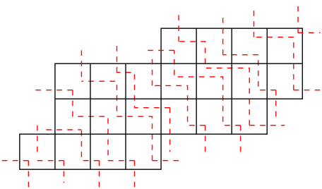
Figure 5: Extended links for the skew shape $8874/411$

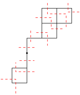
Figure 6: Extended links for the skew shape $43111/2211$

We thus have the following situation. Write $S_{i}$ as short for $S_{f_{i}}$, so $\tau(S_{i})=e_{i}$ and $\beta(S_{i})=f_{i}$. Let

$$\overline{\mathrm{code}}(\lambda/\mu)=\left(\begin{array}[]{cccc}c_{1}&c_{2}&\cdots&c_{k}\\ d_{1}&d_{2}&\cdots&d_{k}\end{array}\right).$$ (15)

It is easy to see that $S_{i}$ is a left snake if and only if $(c_{i},d_{i})=(1,0)$. In this case, if $S_{i}$ has length $2m$ then

$$m+1=\#\{j>i\,:\,(c_{j},d_{j})=(0,1)\}-\#\{j>i\,:\,(c_{j},d_{j})=(1,0)\}.$$ (16)

Similarly $S_{i}$ is a right snake if and only if $(c_{i},d_{i})=(0,1)$; and if $S_{i}$ has length $2m$ then

$$m+1=\#\{j<i\,:\,(c_{j},d_{j})=(1,0)\}-\#\{j<i\,:\,(c_{j},d_{j})=(0,1)\}.$$ (17)

4.3 Proposition.   The snake sequence $\mathrm{SS}(\lambda/\mu)=q_{1}q_{2}\cdots q_{k}$ is “well-parenthesized” in the following sense. There exists a (unique) set ${\cal P}(\lambda/\mu)=\{(u_{1},v_{1}),\dots,(u_{r},v_{r})\}$, where $r=\mathrm{rank}(\lambda/\mu)$, such that:

1. The $u_{i}$’s and $v_{i}$’s are distinct integers.

2. $1\leq u_{i}<v_{i}\leq k$

3. $q_{u_{i}}=L_{t}$ and $q_{v_{i}}=R_{t}$ for some $t$ (depending on $i$)

4. For no $i$ and $j$ do we have $u_{i}<u_{j}<v_{i}<v_{j}$.

Proof. Equations (3) and (4) assert that for any $1\leq i\leq k$ we have

$$\#\{j\,:\,1\leq j\leq i,\ q_{j}=L_{s}\ \mbox{for some}\ s\}\geq\#\{j\,:\,1\leq j\leq i,\ q_{j}=R_{s}\ \mbox{for some}\ s\},$$ (18)

and that the total number of $L$’s in $\mathrm{SS}(\lambda/\mu)$ equals the total number of $R$’s. It now follows from a standard bijection (e.g., [11, solution to Exer. 6.19(n) and (o)]) that there is a unique set ${\cal P}(\lambda/\mu)$ satisfying (a), (b), and (d). But (c) is then a consequence of equations (16) and (17). $\ \Box$

We can depict the set ${\cal P}(\lambda/\mu)$ by drawing arcs above the terms of $\mathrm{SS}(\lambda/\mu)$, such that the left and right endpoints of an arc are some $L_{t}$ and $R_{t}$, and such that the arcs are noncrossing. For instance,

$${\cal P}(8874/411)=\{(1,12),(3,11),(4,5),(8,9)\},$$

as illustrated in Figure 7.

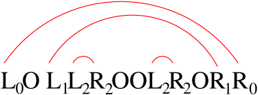
Figure 7: Parenthesization of the snake sequence $\mathrm{SS}(8874/411)$

Let $\mathrm{SS}(\lambda/\mu)=q_{1}q_{2}\cdots q_{k}$ as in Proposition 6, and define an interval set of $\lambda/\mu$ to be collection ${\cal I}$ of $r$ ordered pairs,

$${\cal I}=\{(u_{1},v_{1}),\dots,(u_{r},v_{r})\},$$

satisfying the following conditions:

• The $u_{i}$’s and $v_{i}$’s are distinct integers.

• $1\leq u_{i}<v_{i}\leq k$

• $q_{u_{i}}=L_{s}$ and $q_{v_{i}}=R_{t}$ for some $s$ and $t$ (depending on $i$)

Thus ${\cal P}(\lambda/\mu)$ is itself an interval set. Figure 8 illustrates the interval set $\{(1,5),(3,12),(4,9),(8,11)\}$ of the skew shape $8874/411$. Let is$(\lambda/\mu)$ denote the number of interval sets of $\lambda/\mu$.

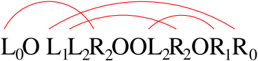
Figure 8: An interval set of the skew shape $8874/411$

4.4 Theorem.   Let $T_{1},\dots,T_{r}$ be the left snakes (or right snakes) of $\lambda/\mu$. Then

$$\mathrm{is}(\lambda/\mu)=\prod_{i=1}^{r}\left(1+\frac{\ell(T_{i})}{2}\right).$$

Proof. Let $\mathrm{SS}(\lambda/\mu)=q_{1}q_{2}\cdots q_{k}$. Let $q_{u_{1}},\dots,q_{u_{r}}$ be the positions of the terms $L_{s}$, with $u_{1}<\cdots<u_{r}$. Let $q_{u_{i}}=L_{m_{i}}$. We can obtain an interval set by pairing $q_{u_{r}}$ with some $R_{s}$ to the right of $q_{u_{r}}$, then pairing $q_{u_{r-1}}$ with some $R_{s}$ to the right of $q_{u_{r-1}}$ not already paired, etc. By equation (16) the number of choices for pairing $q_{u_{i}}$ is just $m_{i}+1$, and the proof follows. $\ \Box$

We are now in a position to count the number of minimal border strip decompositions and minimal border strip tableaux of shape $\lambda/\mu$. Let us denote this latter number by mbst$(\lambda/\mu)$.

4.5 Theorem.   Let $\mathrm{rank}(\lambda/\mu)=r$. Then

$$\mathrm{mbsd}(\lambda/\mu) = \mathrm{is}(\lambda/\mu)^{2}$$ (19)

$$\mathrm{mbst}(\lambda/\mu) = r!\,\mathrm{is}(\lambda/\mu).$$ (20)

Proof. Equation (19) is an immediate consequence of Proposition 4 and Theorem 8 (using that in Theorem 8 we can take $T_{1},\cdots,T_{r}$ to consist of either all left snakes or all right snakes).

To prove equation (20) we use Proposition 3. Let

$$\overline{\mathrm{code}}(\lambda/\mu)=\begin{array}[]{cccc}c_{1}&c_{2}&\cdots&c_{k}\\ d_{1}&d_{2}&\cdots&d_{k}\end{array}$$

and let $r=\mathrm{rank}(\lambda/\mu)$. It follows from Proposition 3 that a minimal border strip tableau of shape $\lambda/\mu$ is equivalent to choosing a sequence $(u_{1},v_{1}),\dots$, $(u_{r},v_{r})$ where $1\leq u_{i}<v_{i}\leq k$, $c_{u_{i}}=1$, $c_{v_{i}}=0$, the $u_{i}$’s and $v_{i}$’s are distinct, and then successively changing $(u_{i},v_{i})$ from $(1,0)$ to $(0,1)$, so that at the end we obtain the sequence $d_{1},\dots,d_{k}$. Since there are exactly $r$ pairs $(c_{i},d_{i})$ equal to $(0,1)$ and $r$ pairs equal to $(1,0)$, the condition that we end up with $d_{1},\dots,d_{k}$ is equivalent to $d_{u_{i}}=0$ and $d_{v_{i}}=1$. Hence the possible sets $\{(u_{1},v_{1}),\dots,(u_{r},v_{r})\}$ are just the interval sets of $\lambda/\mu$. There are is$(\lambda/\mu)$ ways to choose an interval set and $r!$ ways to linearly order its elements, so the proof follows. $\ \Box$

As discussed in the above proof, every interval set ${\cal I}$ of $\lambda/\mu$ gives rise to $r!$ minimal border strip tableaux $T$ of shape $\lambda/\mu$. The set of border strips appearing in such a tableau is a border strip decomposition $D$ of $\lambda/\mu$. Extending our terminology that $T$ and $D$ correspond to each other, we will say that ${\cal I}$, $D$, and $T$ all correspond to each other.

How many of the above $r!$ border strip decompositions corresponding to ${\cal I}$ are distinct? Rather remarkably, the number is is$(\lambda/\mu)$, independent of the interval set ${\cal I}$. This is a consequence of Theorem 8 below. Our proof of this result is best understood in the context of posets. Let $P$ be a finite poset with $p$ elements $x_{1},\dots,x_{p}$. A bijection $f:P\rightarrow[p]=\{1,2,\dots,p\}$ is called a dropless labeling of $P$ if we never have $f^{-1}(i+1)<f^{-1}(i)$. Let inc$(P)$ denote the incomparability graph of $P$, i.e, the vertex set of inc$(P)$ is $\{x_{1},\dots,x_{p}\}$, with an edge between $x_{i}$ and $x_{j}$ if and only if $x_{i}$ and $x_{j}$ are incomparable in $P$. The next result is implicit in [5, Thm. 2] and [3, Theorem on p. 322] (namely, in [5, Th. 2] put $x=-1$ and in [3, Theorem on p. 322] put $\lambda=-1$, and use (22) below) and explicit in [12, Thm. 4.12]. For the sake of completeness we repeat the essence of the proof in [12].

4.6 Lemma.   The number dl$(P)$ of dropless labelings of $P$ is equal to the number ao$(P)$ of acyclic orientations of inc$(P)$.

Proof. Given the dropless labeling $f:P\rightarrow[p]$, define an acyclic orientation $\mathfrak{o}=\mathfrak{o}(f)$ as follows. If $x_{i}x_{j}$ is an edge of inc$(P)$, then let $x_{i}\rightarrow x_{j}$ in $\mathfrak{o}$ if $f(x_{i})<f(x_{j})$, and let $x_{j}\rightarrow x_{i}$ otherwise. Clearly $\mathfrak{o}$ is an acyclic orientation of inc$(P)$. Conversely, let $\mathfrak{o}$ be an acyclic orientation of inc$(P)$. The set of sources (i.e., vertices with no arrows into them) form a chain in $P$ since otherwise two are incomparable, so there is an arrow between them that must point into one of them. Let $x$ be the minimal element of this chain, i.e., the unique minimal source. If $f$ is a dropless labeling of $P$ with $\mathfrak{o}=\mathfrak{o}(f)$, then we claim $f(x)=1$. Suppose to the contrary that $f(x)=i>1$. Let $j$ be the largest integer satisfying $j<i$ and $y:=f^{-1}(j)\not<x$. Note that $j$ exists since $f^{-1}(1)>x$. We must have $y>x$ since $x$ is a source. But then $f^{-1}(j+1)\leq x<y=f^{-1}(j)$, contradicting the fact that $f$ is dropless. Thus we can set $f(x)=1$, remove $x$ from inc$(P)$, and proceed inductively to construct a unique $f$ satisfying $\mathfrak{o}=\mathfrak{o}(f)$. $\ \Box$

Now given any set

$${\cal I}=\{(u_{1},v_{1}),\dots,(u_{r},v_{r})\}$$ (21)

with $u_{i}<v_{i}$, define a partial order $P_{{\cal I}}$ on ${\cal I}$ by setting $(u_{i},v_{i})<(u_{j},v_{j})$ if $v_{i}<u_{j}$. If we regard the pairs $(u_{i},v_{i})$ as closed intervals $[u_{i},v_{i}]$ in $\mathbb{R}$, then $P_{{\cal I}}$ is just the interval order corresponding to these intervals (e.g., [4][13]).

4.7 Lemma.   Let ${\cal I}$ be as in equation (21). For $1\leq i\leq r$ let

$$\varphi(i)=\#\{j\,:\,v_{j}>v_{i}\}-\#\{j\,:\,u_{j}>v_{i}\}.$$

Then

$$\mathrm{dl}(P_{{\cal I}})=(\varphi(1)+1)(\varphi(2)+1)\cdots(\varphi(r)+1).$$

Proof. Let $\chi_{{\cal I}}(q)$ denote the chromatic polynomial of the graph inc$(P_{{\cal I}})$. We may suppose that the elements of ${\cal I}$ are indexed so that $v_{1}>v_{2}>\cdots>v_{r}$. We can properly color the vertices of inc$(P_{{\cal I}})$ (i.e., adjacent vertices have different colors) in $q$ colors as follows. First color vertex $(u_{1},v_{1})$ in $q$ ways. Suppose that vertices $(u_{1},v_{1}),\dots,(u_{i},v_{i})$ have been colored, where $i<r$. Now for $1\leq j\leq i$, $(u_{i+1},v_{i+1})$ is incomparable in $P_{{\cal I}}$ to $(u_{j},v_{j})$ if and only $v_{i+1}>u_{j}$. These vertices $(u_{j},v_{j})$ form an antichain in $P_{{\cal I}}$; else either some $v_{j}<v_{i+1}$ or some $u_{j}>v_{i+1}$. The number of these vertices is $\varphi(i+1)$. Since they form a a clique in inc$(P_{{\cal I}})$ there are exactly $q-\varphi(i+1)$ ways to color vertex $(u_{i+1},v_{i+1})$, independent of the colors previously assigned. It follows that

$$\chi_{{\cal I}}(q)=\prod_{i=1}^{r}(q-\varphi(i+1)).$$

For any graph $G$ with $r$ vertices it is known [10] that

$$\mathrm{ao}(G)=(-1)^{r}\chi_{G}(-1).$$ (22)

Hence

$$\mathrm{ao}(\mathrm{inc}(P_{{\cal I}}))=\prod_{i=1}^{r}(\varphi(i)+1).$$

The proof follows from Lemmas 8 and 8. $\ \Box$

Note. The fact (shown in the above proof) that we can order the vertices of inc$(P_{{\cal I}})$ so that each vertex is adjacent to a set of previous vertices forming a clique is equivalent to the statement that the incomparability graph of an interval order is chordal. Note that the above proof shows that for any interval order $P$ coming from intervals $[u_{1},v_{1}],\dots,[u_{r},v_{r}]$, the chromatic polynomial of inc$(P)$ depends only on the sets $\{u_{1},\dots,u_{r}\}$ and $\{v_{1},\dots,v_{r}\}$.

We now come to the result mentioned in the paragraph before Lemma 8.

4.8 Theorem.   Let ${\cal I}$ be an interval set of $\lambda/\mu$, thus giving rise to $r!$ minimal border strip tableaux of shape $\lambda/\mu$. Then the number of distinct border strip decompositions that correspond to these $r!$ border strip tableaux is is$(\lambda/\mu)$.

Proof. Let $(u_{i},v_{i}),(u_{j},v_{j})\in{\cal I}$. We say that $(u_{i},v_{i})$ and $(u_{j},v_{j})$ overlap if $[u_{i},v_{i}]\cap[u_{j},v_{j}]\neq\emptyset$, where $[a,b]=\{u_{i},u_{i}+1,\dots,v_{i}\}$. Two linear orderings $\pi$ and $\sigma$ of ${\cal I}$ correspond to the same border strip decomposition if and only if any two overlapping elements $(u_{i},v_{i})$ and $(u_{j},v_{j})$ appear in the same order in $\pi$ and $\sigma$. Suppose that $\pi$ is given by the linear ordering

$$\pi=[(u_{i_{1}},v_{i_{1}}),\dots,(u_{i_{r}},v_{i_{r}})].$$ (23)

If $(u_{i_{m}},v_{i_{m}})$ and $(u_{i_{m+1}},v_{i_{m+1}})$ are consecutive terms of $\pi$ which do not overlap and if $i_{m}>i_{m+1}$, then we can transpose the two terms without affecting the border strip decomposition defined by $\pi$. By a series of such transpositions we can put $\pi$ in the “canonical form” where consecutive nonoverlapping pairs appear in increasing order of their subscripts. The number of distinct border strip decompositions that correspond to the $r!$ permutations $\pi$ is the number of $\pi$ that are in canonical form. Let $\pi$ be given by (23), and define $f:P_{{\cal I}}\rightarrow[r]$ by $f(u_{i_{m}},v_{i_{m}})=m$. Then $\pi$ is in canonical form if and only if $f$ is dropless. Comparing equation (16), Theorem 8, and Lemma 8 completes the proof. $\ \Box$

Note that Theorem 8 gives a refinement of equation (19), since we have partitioned the is$(\lambda/\mu)^{2}$ minimal border strip decompositions of $\lambda/\mu$ into is$(\lambda/\mu)$ blocks, each of size is$(\lambda/\mu)$.

Now let ${\cal I}=\{(u_{1},v_{1}),\dots,(u_{i},v_{i})\}$ be an interval set of $\lambda/\mu$. Define the type of ${\cal I}$ to be the partition $\sigma$ whose parts are the integers $v_{1}-u_{1},\dots,v_{r}-u_{r}$. Hence by Proposition 3 $\sigma$ is also the type of any of the border strip decompositions corresponding to ${\cal I}$. Let is${}_{\sigma}(\lambda/\mu)$ denote the number of interval sets of $\lambda/\mu$ of type $\sigma$, and let mbsd${}_{\sigma}(\lambda/\mu)$ denote the number of minimal border strip decompositions of $\lambda/\mu$ of type $\sigma$. The following result is a refinement of equation (19).

4.9 Corollary.   Let $N=|\lambda/\mu|$. For any partition $\sigma\vdash N$, we have

$$\mathrm{mbsd}_{\sigma}(\lambda/\mu)=\mathrm{is}_{\sigma}(\lambda/\mu)\mathrm{is}(\lambda/\mu).$$

Proof. Immediate consequence of Theorem 8 and the observation above that type$({\cal I})=\mathrm{type}({\mbox{\boldmath$D$}})$ for any interval set ${\cal I}$ and border strip decomposition $D$ corresponding to ${\cal I}$. $\ \Box$

We can improve the above corollary by explicitly partitioning the minimal border strip decompositions of $\lambda/\mu$ into is$(\lambda/\mu)$ blocks, each of which contains exactly mbsd${}_{\sigma}(\lambda/\mu)$ border strip decompositions of type $\sigma$.

4.10 Theorem.   For each right snake $S$ of $\lambda/\mu$ fix a set $F_{S}$ of $\ell(S)/2$ links of $S$, no two consecutive, and let $F=\bigcup_{S}F_{S}$. Let $Q_{F}$ be the set of all minimal border strip decompositions $D$ of $\lambda/\mu$ which use the links in $Q_{F}$. Then for each $\sigma\vdash N=|\lambda/\mu|$, $Q_{F}$ contains exactly is${}_{\sigma}(\lambda/\mu)$ minimal border strip decompositions of type $\sigma$.

Figure 9 illustrates Theorem 8 for the case $\lambda/\mu=332/1$. We are using dots rather than squares in the diagram of $\lambda/\mu$. The first column shows the right snakes, with the choice of links as a solid line and the remaining links as dashed lines. The first row shows the same for the left snakes. The remaining 16 entries are the minimal border strip decompositions of $\lambda/\mu$ using the right snake links for that row and the left snake links for that column. Theorem 8 asserts that each row (and hence by symmetry each column) contains the same number of minimal border strip decompositions of each type, viz., one of type $(5,1,1)$, two of type $(4,2,1)$, and one of type $(3,2,2)$. For general $\lambda/\mu$ there will also be snakes of odd length $2m-1$ yielding $m$ links that must be used in every minimal border strip decomposition.

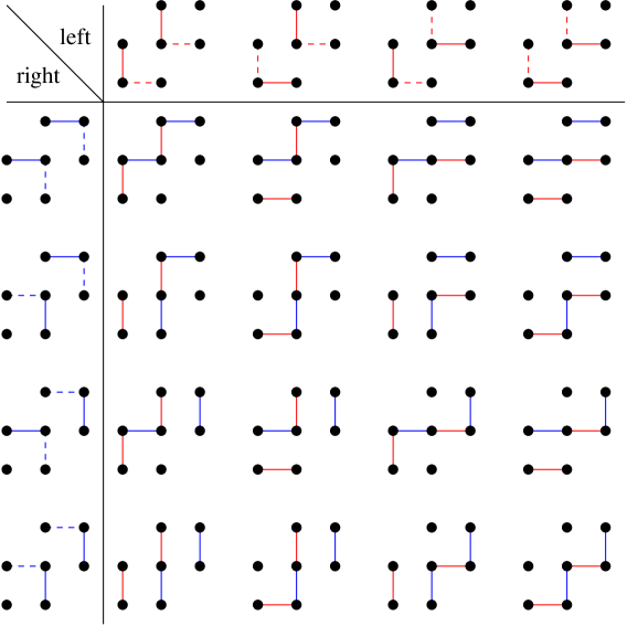
Figure 9: Minimal border strip decompositions of the skew shape $332/1$

Proof of Theorem 8. Let ${\cal I}$ be an interval set of $\lambda/\mu$ of type $\sigma$. By Theorem 8 there are exactly is$(\lambda/\mu)$ border strip decompositions (all of type $\sigma$) corresponding to ${\cal I}$.

Claim. Any two of the above is$(\lambda/\mu)$ border strip decompositions $D$ have a different set of left links and a different set of right links.

By symmetry it suffices to show that any two, say $D$ and ${\mbox{\boldmath$D$}}^{\prime}$, have a different set of left links. Let $\overline{\mathrm{code}}(\lambda/\mu)$ be given by (15), and let $S_{i}=S_{f_{i}}$ as defined just before (15). Thus $S_{i}$ is a left snake if and only if $(c_{i},d_{i})=(0,1)$. Moreover, if $S_{i}$ is a left snake and ${\cal I}=\{(u_{1},v_{1}),\dots,(u_{r},v_{r})\}$ is any interval set for $\lambda/\mu$, then it follows from (16) that $\ell(S_{i})=2m$ where

$$m=\#\{j\,:\,u_{j}<i<v_{j}\}.$$

Let $j_{1},\dots,j_{m}$ be those $j$ for which $u_{j}<i<v_{j}$. In a linear ordering $\pi$ of ${\cal I}$ there are $m+1$ choices for how many of the pairs $(u_{j_{s}},v_{j_{s}})$ precede $(u_{i},v_{i})$. The linear ordering $\pi$ defines a border strip tableau with corresponding border strip decomposition $D$. In turn $D$ is defined by a choice of a maximum number of links, no two consecutive, from each left and right snake. The choices of links from the snake $S_{i}$ are equivalent to choosing the number of pairs $(u_{j_{s}},v_{j_{s}})$ preceding $(u_{i},v_{i})$ in $\pi$, since $S_{i}$ intersects precisely the border strips $B_{i}$ and $B_{j_{s}}$ corresponding to $(u_{i},v_{i})$ and the $(u_{j_{s}},v_{j_{s}})$’s, and the position of $B_{i}$ within the snake determines the unique two consecutive unused links of the snake $S_{i}$ extended by adding one square in each direction. Moreover, $B_{i}$ will be the unique border strip whose initial square (reading from lower-left to upper-right) begins on $S_{i}$. As an example see Figure 10, which shows the skew shape $\lambda/\mu=66554/1$ with the left snake $S_{6}$ shaded. There are four border strips intersecting $S_{6}$, and the third one (reading from bottom-right to upper-left) begins on the square $(2,3)$ of $S_{6}$. The two links of $S_{6}$ involving this square are not used in the border strip decomposition $D$.

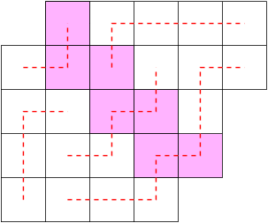
Figure 10: Intersection of border strips with a left snake

A dropless labeling of ${\cal I}$ is uniquely determined by specifying for each left snake $S_{i}$ how many of the $(u_{j_{s}},v_{j_{s}})$’s, as defined above, precede $(u_{i},v_{i})$; for we can inductively determine, preceding from left-to-right in $\overline{\mathrm{code}}(\lambda/\mu)$, the relative order of any pair $(u_{i},v_{i})$ and $(u_{j},v_{j})$ of elements which cross, while all remaining ambiguities in the labeling are resolved by the dropless condition. Thus the is$(\lambda/\mu)$ dropless labelings of ${\cal I}$ define border strip tableaux of shape $\lambda/\mu$ and type $\sigma$, no two of which have the same left links. Since these border strip tableaux correspond to different border strip decompositions (by the proof of Theorem 8), the proof of the claim follows.

By the claim, for each interval set ${\cal I}$ the is$(\lambda/\mu)$ border strip decompositions corresponding to ${\cal I}$ all have the same type and belong to different $Q_{F}$’s. Since there are is$(\lambda/\mu)$ different $Q_{F}$’s it follows that each $Q_{F}$ contains exactly is${}_{\sigma}(\lambda/\mu)$ minimal border strip decompositions of type $\sigma$, as was to be proved. $\ \Box$

Another way to state Theorem 8 is as follows. Let $A$ be the square matrix whose columns (respectively, rows) are indexed by the maximum size sets $G$ (respectively, $F$) of links, no two consecutive, of right snakes (respectively, left snakes) of $\lambda/\mu$. The entry $A_{FG}$ is defined to be the minimal border strip decomposition of $\lambda/\mu$ using the links $F$ and $G$. Figure 9 shows this matrix for $\lambda/\mu=332/1$. Let $t=\mathrm{is}(\lambda/\mu)$ and let ${\cal I}_{1},\dots,{\cal I}_{t}$ be the interval sets of $\lambda/\mu$. If the border strip decomposition $A_{FG}$ corresponds to ${\cal I}_{j}$, then let $L$ be the matrix obtained by replacing $A_{FG}$ with the integer $j$. Then the matrix $L$ is a Latin square, i.e., every row and every column is a permutation of $1,2,\dots,t$. For instance, when $\lambda/\mu=332/1$ the interval sets are

$$\begin{array}[]{ll}{\cal I}_{1}=\{(1,6),(2,3),(4,5)\},&{\cal I}_{2}=\{(1,3),(2,6),(4,5)\}\\ {\cal I}_{3}=\{(1,5),(2,3),(4,6)\},&{\cal I}_{4}=\{(1,3),(2,5),(4,6)\}.\end{array}$$

The matrix $A$ of Figure 9 becomes the Latin square

$$L=\left[\begin{array}[]{cccc}1&2&3&4\\ 2&1&4&3\\ 3&4&1&2\\ 4&3&2&1\end{array}\right].$$

5 An application to the characters of $\mathfrak{S}_{n}$.

Expand the skew Schur function $s_{\lambda/\mu}$ in terms of power sums as in equation (7). Define deg$(p_{i})=1$, so deg$(p_{\nu})=\ell(\nu)$. As mentioned after (7), the Murnaghan-Nakayama rule (10) implies that if $p_{\nu}$ appears in $s_{\lambda/\mu}$ then deg$(p_{\nu})\geq r=\mathrm{rank}(\lambda/\mu)$. In fact, at least one such $p_{\nu}$ actually appears in $s_{\lambda/\mu}$, viz., let $\nu_{1}$ be the length of the longest border strip $B_{1}$ of $\lambda/\mu$, then $\nu_{2}$ the length of the longest border strip $B_{2}$ of $\lambda/\mu-B_{1}$, etc. All border strip tableaux of $\lambda/\mu$ of type $\nu$ involve the same set of border strips, so there is no cancellation in the right-hand side of (10). Hence the coefficient of $p_{\nu}$ in $s_{\lambda/\mu}$ in nonzero. (See [11, Exer. 7.52] for the case $\mu=\emptyset$.) Let us write $\hat{s}_{\lambda/\mu}$ for the lowest degree part of $s_{\lambda/\mu}$, so

$$\hat{s}_{\lambda/\mu}=\sum_{\nu\,:\,\ell(\nu)=r}z_{\nu}^{-1}\chi^{\lambda/\mu}(\nu)p_{\nu},$$ (24)

where $r=\mathrm{rank}(\lambda/\mu)$. Also write For instance,

$$s_{332/1}=\frac{1}{120}p_{1}^{7}-\frac{1}{12}p_{1}^{4}p_{3}+\frac{1}{24}p_{1}^{3}p_{2}^{2}+\frac{1}{5}p_{1}^{2}p_{5}-\frac{1}{4}p_{1}p_{2}p_{4}+\frac{1}{12}p_{2}^{2}p_{3}.$$

Hence

$$\hat{s}_{332/1} = \frac{1}{5}p_{1}^{2}p_{5}-\frac{1}{4}p_{1}p_{2}p_{4}+\frac{1}{12}p_{2}^{2}p_{3}$$

$$= \tilde{p}_{1}^{2}\tilde{p}_{5}-2\tilde{p}_{1}\tilde{p}_{2}\tilde{p}_{4}+\tilde{p}_{2}^{2}\tilde{p}_{3}.$$

If ${\cal I}=\{(w_{1},y_{1}),\dots,(w_{r},y_{r})\}$ is an interval set, then let $c({\cal I})$ denote the number of crossings of ${\cal I}$, i.e., the number of pairs $(i,j)$ for which $w_{i}<w_{j}<y_{i}<y_{j}$. Moreover, let ${\cal P}(\lambda/\mu)=\{(u_{1},v_{1}),\dots,(u_{r},v_{r})\}$ be as in Proposition 6, and let

$$\overline{\mathrm{code}}(\lambda/\mu)=\begin{array}[]{cccc}c_{1}&c_{2}&\cdots&c_{k}\\ d_{1}&d_{2}&\cdots&d_{k}\end{array}.$$

For $1\leq i\leq r$ define

$$z(i) = \#\{j\,:\,u_{i}<j<v_{i},\ c_{j}=0\}$$

$$z(\lambda/\mu) = z(1)+z(2)+\cdots+z(r).$$

It is easy to see (see the proof of Theorem 5 for more details) that $z(\lambda/\mu)$ is just the height $\mathrm{ht}({\mbox{\boldmath$T$}})$ of a “greedy border strip tableau” $T$ of shape $\lambda/\mu$ obtained by starting with $\lambda/\mu$ and successively removing the largest possible border strip. (Although $T$ may not be unique, the set of border strips appearing in $T$ are unique, so ht$({\mbox{\boldmath$T$}})$ is well-defined.)

5.1 Lemma.   Let ${\cal I}$ be an interval set of $\lambda/\mu$. If $T$ and $T^{\prime}$ are two border strip tableaux corresponding to ${\cal I}$, then $\mathrm{ht}({\mbox{\boldmath$T$}})\equiv\mathrm{ht}({\mbox{\boldmath$T$}}^{\prime})\ (\mathrm{mod}\ 2)$.

Proof. When we remove a border strip $B$ of size $p$ from a skew shape $\alpha/\beta$ with $\mathrm{code}(\alpha)=\cdots c_{0}c_{1}c_{2}\cdots$, then by Proposition 3 we replace some $(c_{i},c_{i+p})=(1,0)$ with $(0,1)$. It is easy to check (and is also equivalent to the discussion in [1, top of p. 3]) that

$$\mathrm{ht}(B)=\#\{h\,:\,i<h<i+p,\ c_{h}=0\}.$$ (25)

Suppose we have $(c_{i},c_{i+p})=(c_{j},c_{j+q})=(1,0)$, where the four numbers $c_{i},c_{i+p},c_{j},c_{j+q}$ are all distinct. Let $B_{1}$ be the the border strip corresponding to $(i,i+p)$ and $B_{2}$ the border strip corresponding to $(j,j+q)$ after $B_{1}$ has been removed. Similarly let $B^{\prime}_{1}$ correspond to $(j,j+q)$ and $B^{\prime}_{2}$ to $(i,i+p)$ after $B^{\prime}_{1}$ has been removed. If $i+p<j$ or $j+q<i$ then $B_{1}=B^{\prime}_{2}$ and $B_{2}=B^{\prime}_{1}$, so $\mathrm{ht}(B_{1})+\mathrm{ht}(B_{2})=\mathrm{ht}(B^{\prime}_{1})+\mathrm{ht}(B^{\prime}_{2})$. In particular,

$$\mathrm{ht}(B_{1})+\mathrm{ht}(B_{2})\equiv\mathrm{ht}(B^{\prime}_{1})+\mathrm{ht}(B^{\prime}_{2})\ (\mathrm{mod}\ 2).$$ (26)

If $c_{i}<c_{j}<c_{i+p}<c_{j+q}$, then using (25) we see that $\mathrm{ht}(B_{1})=\mathrm{ht}(B^{\prime}_{2})-1$ and $\mathrm{ht}(B_{2})=\mathrm{ht}(B^{\prime}_{1})-1$ so again (26) holds. Similarly it is easy to check (26) in all remaining cases.

Iterating the above argument and using the fact that every permutation is a product of adjacent transpositions completes the proof. $\ \Box$

5.2 Theorem.   For any skew shape $\lambda/\mu$ of rank $r$ we have

$$\hat{s}_{\lambda/\mu}=(-1)^{z(\lambda/\mu)}\sum_{{\cal I}=\{(u_{1},v_{1}),\dots,(u_{r},v_{r})\}}(-1)^{c({\cal I})}\prod_{i=1}^{r}\tilde{p}_{v_{i}-u_{i}},$$ (27)

where ${\cal I}$ ranges over all interval sets of $\lambda/\mu$.

Proof. Let $\cal{I}$ be an interval set of $\lambda/\mu$, and let $T$ be a border strip tableau corresponding to ${\cal I}$. We claim that

$$\mathrm{ht}({\mbox{\boldmath$T$}})\equiv z(\lambda/\mu)+c({\cal I})\ (\mathrm{mod}\ 2).$$ (28)

The proof of the claim is by induction on $c({\cal I})$.

First note that by Lemma 5, it suffices to prove the claim for some $T$ corresponding to each ${\cal I}$. Suppose that $c({\cal I})=0$, so ${\cal I}={\cal P}$. Let $T$ be a greedy border strip tableau as defined before Lemma 5. The corresponding interval set is just ${\cal P}$, the unique interval set without crossings, since if $u_{i}<u_{j}<v_{i}<v_{j}$ we would pick the border strip corresponding to $(u_{i},v_{j})$ rather than $(u_{i},v_{i})$ or $(u_{j},v_{j})$. Since by (25) we have $z(\lambda/\mu)=\mathrm{ht}({\mbox{\boldmath$T$}})$, equation (28) holds when $c({\cal I})=0$.

Now let $c({\cal I})>0$. Suppose that $(u_{i},v_{i})$ and $(u_{j},v_{j})$ define a crossing in ${\cal I}$, say $u_{i}<u_{j}<v_{i}<v_{j}$. Let ${\cal I}^{\prime}$ be obtained from ${\cal I}$ by replacing $(u_{i},v_{i})$ and $(u_{j},v_{j})$ with $(u_{i},v_{j})$ and $(u_{j},v_{i})$. It is easy to see that $c({\cal I})-c({\cal I}^{\prime})$ is an odd positive integer. By the induction hypothesis we may assume that (28) holds for ${\cal I}^{\prime}$. Let ${\mbox{\boldmath$T$}}^{\prime}$ be a border strip tableau corresponding to ${\cal I}^{\prime}$ such that the border strips $B_{1}$ and $B_{2}$ indexed by $(u_{1},v_{1})$ and $(u_{2},v_{2})$ are removed first (say in the order $B_{1},B_{2}$). Let $T$ be the border strip tableau that differs from ${\mbox{\boldmath$T$}}^{\prime}$ by replacing $B_{1},B_{2}$ with the border strips indexed by $(u_{j},v_{i})$ and $(u_{i},v_{j})$. It is straightforward to verify, using (25) or a direct argument, that $\mathrm{ht}({\mbox{\boldmath$T$}})$ and $\mathrm{ht}({\mbox{\boldmath$T$}}^{\prime})$ differ by an odd integer. Hence (28) holds for ${\cal I}$, and the proof of the claim follows by induction.

Now let $\ell(\nu)=r$ and $m_{i}(\nu)=\#\{j\,:\,\nu_{j}=i\}$, the number of parts of $\nu$ equal to $i$. Since $z_{\nu}=1^{\nu_{1}}\nu_{1}!\,2^{\nu_{2}}\nu_{2}!\cdots$, we have

$$\hat{s}_{\lambda/\mu} = \sum_{\ell(\nu)=r}z_{\nu}^{-1}\chi^{\lambda/\mu}(\nu)p_{\nu}$$

$$= \sum_{\ell(\nu)=r}\frac{1}{m_{1}(\nu)!\,m_{2}(\nu)!\cdots}\chi^{\lambda/\mu}(\nu)\tilde{p}_{\nu}.$$

Now by the Murnaghan-Nakayama rule we have

$$\chi^{\lambda/\mu}(\nu)=\sum_{{\mbox{\scriptsize\boldmath$T$}}}(-1)^{\mathrm{ht}({\mbox{\scriptsize\boldmath$T$}})},$$

where $T$ ranges over all border strip tableaux of shape $\lambda/\mu$ and some fixed type $\alpha=(\alpha_{1},\dots,\alpha_{r})$ whose decreasing rearrangement is $\nu$. Since there are $r!/m_{1}(\nu)!m_{2}(\nu)!\cdots$ different permutations $\alpha$ of the entries of $\nu$, we have

$$\chi^{\lambda/\mu}(\nu)=\frac{m_{1}(\nu)!\,m_{2}(\nu)!\cdots}{r!}\sum_{{\mbox{\scriptsize\boldmath$T$}}}(-1)^{\mathrm{ht}({\mbox{\scriptsize\boldmath$T$}})},$$

where $T$ now ranges over all border strip tableaux of shape $\lambda/\mu$ whose type is some permutation $\alpha$ of $\nu$. By Theorem 8, Proposition 3, and equation (28) we then have

$$\chi^{\lambda/\mu}(\nu)=\frac{m_{1}(\nu)!\,m_{2}(\nu)!\cdots}{r!}\left(r!\sum_{{\cal I}\,:\,\mathrm{type}({\cal I})=\nu}(-1)^{z(\lambda/\mu)+c({\cal I})}\right),$$ (29)

where ${\cal I}$ ranges over all interval sets of $\lambda/\mu$ of type $\nu$, and the proof follows. $\ \Box$

Let us remark that just as in the Murnaghan-Nakayama rule, cancellation can occur in the sum on the right-hand side of (27). For instance, if $\lambda/\mu=4442/11$ then there is one interval set of type $(6,3,2,1)$ with one crossing and one with two crossings.

The following corollary follows immediately from equation (29).

5.3 Corollary.   Let $\lambda/\mu$ be a skew shape of rank $r$ and let $\ell(\nu)=r$. Then $\chi^{\lambda/\mu}(\nu)$ is divisible by $m_{1}(\nu)!\,m_{2}(\nu)!\cdots$.

Let $A=(a_{ij})$ be an array of real numbers with $1\leq i<j\leq 2r$. Recall that the Pfaffian Pf$(A)$ may be defined by (e.g. [6, p. 616])

$$\mathrm{Pf}(A)=\sum_{\pi}(-1)^{c(\pi)}a_{i_{1}j_{1}}\cdots a_{i_{r}j_{r}},$$

where the sum is over all partitions $\pi$ of $\{1,2,\dots,2r\}$ into two element blocks $i_{k}<j_{k}$, and where $c(\pi)$ is the number of crossings of $\pi$, i.e., the number of pairs $h<k$ for which $i_{h}<i_{k}<j_{h}<j_{k}$. Comparing with Theorem 5 gives the following alternative way of writing (27). Let $\mathrm{SS}(\lambda/\mu)=q_{1}q_{2}\cdots q_{k}$; let $u_{1}<u_{2}<\cdots<u_{r}$ be those indices for which $q_{u_{i}}=L_{s}$ for some $s$; and let $v_{1}<v_{2}<\cdots<v_{r}$ be those indices for which $q_{v_{i}}=R_{s}$ for some $s$. Let $w_{1}<w_{2}<\cdots<w_{2r}$ consist of the $u_{i}$’s and $v_{i}$’s arranged in increasing order. Then

$$\hat{s}_{\lambda/\mu}=(-1)^{z(\lambda/\mu)}\mathrm{Pf}(a_{ij}),$$

where

$$a_{ij}=\left\{\begin{array}[]{rl}\tilde{p}_{w_{j}-w_{i}},&\mathrm{if}\ w_{i}=u_{s}\ \mathrm{and}\ w_{j}=v_{t}\ \mbox{for some}\ s<t\\ 0,&\mbox{otherwise.}\end{array}\right.$$

For instance, $\mathrm{SS}(443/2)=L_{0}L_{1}OR_{1}L_{1}R_{1}R_{0}$ and $z(443/2)=2$, whence

$$\hat{s}_{443/2}=\mathrm{Pf}\left(\begin{array}[]{cccccc}&0&\tilde{p}_{3}&0&\tilde{p}_{5}&\tilde{p}_{6}\\ &&\tilde{p}_{2}&0&\tilde{p}_{4}&\tilde{p}_{5}\\ &&&0&0&0\\ &&&&\tilde{p}_{1}&\tilde{p}_{2}\\ &&&&&0\\ &&&&&\end{array}\right).$$

Note that from (11) or (24) we get the following Pfaffianic formula for the coefficient $y(\lambda/\mu)$ of $t^{\mathrm{rank}(\lambda/\mu)}$ in $s_{\lambda/\mu}(1^{t})$:

$$y(\lambda/\mu)=(-1)^{z(\lambda/\mu)}\mathrm{Pf}(b_{ij}),$$

where

$$b_{ij}=\left\{\begin{array}[]{rl}1/(w_{j}-w_{i}),&\mathrm{if}\ w_{i}=u_{s}\ \mathrm{and}\ w_{j}=v_{t}\ \mbox{for some}\ s<t\\ 0,&\mbox{otherwise.}\end{array}\right.$$

Similarly from Theorem 5 there follows

$$y(\lambda/\mu)=(-1)^{z(\lambda/\mu)}\sum_{{\cal I}=\{(u_{1},v_{1}),\dots,(u_{r},v_{r})\}}\frac{(-1)^{c({\cal I})}}{\prod_{i=1}^{r}(v_{i}-u_{i})},$$ (30)

summed over all interval sets ${\cal I}$ of $\lambda/\mu$.

Acknowledgement. I am grateful to Christine Bessenrodt for suggesting the use of Comét codes in the context of skew partitions and for supplying part (d) of Proposition 3, as well as for her careful reading of the original manuscript.

References

- [1] C. Bessenrodt, On hooks of Young diagrams, Ann. Combin. 2 (1998), 103–110.
- [2] C. Bessenrodt, On hooks of skew Young diagrams and bars, Ann. Combin. 5 (2001), 37–49.
- [3] J. P. Buhler and R. L. Graham, A note on the binomial drop polynomial of a poset, J. Combinatorial Theory (A) 66 (1994), 321–326.
- [4] P. C. Fishburn, Interval Orders and Interval Graphs, Wiley, New York, 1985.
- [5] J. R. Goldman, J. T. Joichi, and D. White, Rook theory III. Rook polynomials and the chromatic structure of graphs, J. Combinatorial Theory (B) 25 (1978), 135–142.
- [6] L. Lovász, Combinatorial Problems and Exercises, second ed., North-Holland, Amsterdam, 1993.
- [7] I. G. Macdonald, Symmetric Functions and Hall Polynomials, second ed., Oxford University Press, Oxford, 1995.
- [8] T. Muir, A Treatise on the Theory of Determinants, revised and enlarged by W. H. Metzler, Dover, New York, 1960.
- [9] M. Nazarov and V. Tarasov, On irreducibility of tensor products of Yangian modules associated with skew Young diagrams, preprint, math.QA/0012039.
- [10] R. Stanley, Acyclic orientations of graphs, Discrete Math. 5 (1973), 171–178.
- [11] R. Stanley, Enumerative Combinatorics, vol. 2, Cambridge University Press, New York/Cambridge, 1999.
- [12] E. Steingrimsson, Permutation statistics of indexed and poset permutations, Ph.D. thesis, M.I.T., 1991.
- [13] W. T. Trotter, Combinatorics and Partially Ordered Sets, Johns Hopkins University Press, Baltimore, 1992.