Verification Theorems for Hamilton-Jacobi-Bellman equations

Abstract

We study an optimal control problem in Bolza form and we consider the value function associated to this problem. We prove two verification theorems which ensure that, if a function $W$ satisfies some suitable weak continuity assumptions and a Hamilton-Jacobi-Bellman inequality outside a countably $\mathcal{H}^{n}$-rectifiable set, then it is lower or equal to the value function. These results can be used for optimal synthesis approach.

Key Words: verification theorem, optimal control, HJB equation, value function, viscosity solution.
AMS subject classification: 49K15, 93C15, 49L25.

1. Introduction.

In this paper we consider a control system of the type:

$$\dot{x}=f(t,x,u),\qquad u\in U$$ (1.1)

where $x\in\mathbb{R}^{n}$ is the state, $U\subset\mathbb{R}^{q}$ is the control space and $f$ is the controlled dynamic. Given a target $S\subset\mathbb{R}^{n}$, a running cost $L(t,x,u)$, a final cost $\psi(t,x)$ and an initial condition $(t_{0},x_{0})$, we consider the optimal control problem in Bolza form consisting in minimizing the integral of $L$ summed with the value of $\psi$ at final points for trajectories that start at $x_{0}$ at time $t_{0}$ and reach the target $S$. We define in the usual way the value function $V(t_{0},x_{0})$ to be the infimum of the problem with initial condition $(t_{0},x_{0})$. It is well known that, under special conditions, $V$ satisfies the Hamilton-Jacobi-Bellman equation in viscosity sense [1] and it is the unique solution. Part of the proof is based on the Dynamic Programming Principle.

Therefore given a function $W$ with suitable properties, it is possible to determine if $W$ coincide with the value function, checking if it is a viscosity solution to the HJB equation. This type of theorems, called verification theorems, are useful, for example, when a candidate value function is produced by means of the construction of a synthesis [18]. It is then natural to ask for minimal conditions under which a function $W$ coincides with the value function. If we know that $W$ was obtained via a synthesis then the inequality $W\geq V$ is granted by construction, thus we take this assumption. Then, for $W$ to coincide with the value function, we prove it is sufficient that, outside a rectifiable set of codimension one, both $W$ is differentiable and it satisfies a Hamilton-Jacobi-Bellman inequality in classical sense. Moreover, we make use of only some weak continuity assumptions, already used in [18] to prove optimality of a regular extremal synthesis, see Theorem 5.1 and Theorem 6.1 for details. A first result in this direction can be found in [11], where the HJB inequality is asked outside a locally finite collection of regular manifolds of positive codimension (under more restrictive continuity assumptions). Notice that, for an optimal control problem, if the value function is also semiconcave, it is differentiable outside a countably $\mathcal{H}^{n}$-rectifiable set, see [8].

We start considering the main assumptions for the problem and presenting two technical lemmas, one of which dealing with the cardinality of the intersections between admissible trajectories and a countably $\mathcal{H}^{n}$-rectifiable set, while the other giving some conditions to assure the monotonicity of a real valued function. Also we state, without proofs, two propositions dealing with the properties of the solution to (1.1) and in particular dealing with existence, uniqueness and continuous dependence by data.

Then, in Section 3.​​, we recall briefly the synthesis approach and various results available in the literature for comparison. Some examples of regular optimal synthesis, to which our main results are applicable, are given.

The first case we treat is the problem of finite time. We define a value function as the infimum, over all admissible trajectories reaching the target in finite time. The main result of this part is Theorem 5.1 which permits to verify if the function $W$ is lower or equal than the value function.

Next, we consider the infinite time problem. In this case the value function (6.1) is defined as the infimum of the cost functional over all admissible trajectories reaching the target in infinite time. The main result of this section is Theorem 6.1 which gives sufficient conditions on the function $W$ to ensure the inequality $W\leqslant V$, where $V$ is the value function. In this case, for a technical reason, we consider a suitable neighborhood $S_{1}$ of the target $S$ and we suppose that the final cost $\psi$ is defined on $S_{1}$ in order to give sense to the limit in the definition of the value function (6.1). As a corollary of Theorem 5.1 and Theorem 6.1 we can treat a mixed case (see also [17]), considering at the same time the trajectories reaching the target both in finite time and in infinite time.

A key ingredient for Theorem 5.1 and Theorem 6.1 is the positiveness of the Lagrangian $L$, in order to prevent some bad phenomena such as the permanence of the system for an arbitrary interval of times in a region where $L$ is negative making the value function equal to $-\infty$ as we see in Example 5.1. More precisely, it is not necessary to suppose $L$ positive in the whole space, but some relaxed assumptions can be taken, as we see in Remark 5.4.

This paper ends with an appendix, where we give the definition of a non continuous viscosity solution as in [1] and we state Theorem A.1, which ensures that, under suitable assumptions, the value functions (2.4) and (6.1) are viscosity solutions to the Hamilton-Jacobi-Bellman equation.

Acknowledgments

The author wishes to thank Prof. B. Piccoli, for having proposed him the study of this problem and for his useful advice, and the referees, for their improving suggestions.

2. Preliminaries.

We consider a control system:

$$\dot{x}(t)=f(t,x(t),u(t)),\quad(t,x)\in\Omega,\quad u(t)\in U$$ (2.1)

where

1. $\Omega$ is an open and connected subset of $\mathbb{R}\times\mathbb{R}^{n}$.

2. $U$ is a non-empty subset of $\mathbb{R}^{q}$, for some $q\geqslant 1$, $q\in\mathbb{N}$.

3. $\mathcal{U}=L^{p}(\mathbb{R};U)$ with $1\leqslant p<+\infty$ is the set of admissible controls.

4. $f:\Omega\times U\to\mathbb{R}^{n}$ is measurable in $t$, continuous in $(x,u)$, differentiable in $x$ and, for each $u\in U$, $D_{x}f(\cdot,\cdot,u)$ is bounded on compact sets. Moreover there exists $\varphi_{1}:\mathbb{R}\to\mathbb{R}^{+}$ integrable and for every $K$, compact subset of $\Omega$, there exist a modulus of continuity $\omega_{K}$ and a constant $L_{K}>0$ such that, if $(t,x)\in K$ and $(t,y)\in K$, then for all $u$

   $$\begin{cases}\left|f(t,x,u)-f(t,y,u)\right|\leqslant\omega_{K}(\left|x-y\right|)\\ \left(f(t,x,u)-f(t,y,u)\right)\cdot(x-y)\leqslant L_{K}\left|x-y\right|^{2}\\ \left|f(t,x,u)\right|\leqslant L_{K}(\varphi_{1}(t)+\left|u\right|^{p}).\end{cases}$$ (2.2)

We consider a function $L:\Omega\times U\to\mathbb{R}$ and assume:

1. $L$ is measurable in $t$ and continuous in $(x,u)$. Moreover, there exist $\varphi_{2}:\mathbb{R}\to\mathbb{R}^{+}$ integrable and, for every $R\geqslant 0$, $C_{R}\geqslant 0$ such that

   $$\left|L(t,x,u)\right|\leqslant C_{R}(\varphi_{2}(t)+\left|u\right|^{p}),\quad\left|(t,x)\right|\leqslant R.$$ (2.3)

In this paper we indicate with $x(\,\cdot\,;u,t_{0},x_{0})$ the solution to (2.1) such that $x(t_{0};u,t_{0},x_{0})=x_{0}$. Define the value function:

$$V(t_{0},x_{0}):=\!\!\!\inf_{\begin{subarray}{c}u\in\mathcal{U}\vspace{3pt}\\ (T,x(T;u,t_{0},x_{0}))\in S\end{subarray}}\!\!\!\left\{\int_{t_{0}}^{T}\!\!\!\!\!\!L(s,x(s;u,t_{0},x_{0}),u(s))ds\!+\!\psi(T,x(T;u,t_{0},x_{0}))\right\}$$ (2.4)

where $S$ - the target - is a closed subset of $\mathbb{R}\times\mathbb{R}^{n}$ contained in $\Omega$, $\psi:S\to\mathbb{R}$ is the final cost. We recall the following definition:

Definition 2.1

A subset $A$ of $\Omega$ is a countably $\mathcal{H}^{n}$-rectifiable set if there exist $A_{1}$ and $A_{2}$ such that $A=A_{1}\cup A_{2}$, $A_{1}$ is a finite or countable union of connected $\mathcal{C}^{1}$ submanifolds of positive codimension, and $\mathcal{H}^{n}(A_{2})=0$, where $\mathcal{H}^{k}$ is the $k$-dimensional Hausdorff measure.

3. Examples of syntheses.

In next sections we give sufficient conditions for a candidate value function $W$ to coincide with $V$. Beside some regularity conditions, we ask a HJB inequality outside a countably $\mathcal{H}^{n}$-rectifiable set. This regularity is shared by every function $W$ obtained from a regular synthesis, thus it can be used to prove the optimality of the synthesis itself. In this section we give various examples to which Theorem 5.1 is applicable. First of all, we need some definitions.

Definition 3.1

A synthesis $\Gamma$ is a collection $\{(x_{(\bar{t},\bar{y})}(\cdot),u_{(\bar{t},\bar{y})})\}_{(\bar{t},\bar{y})\in\Omega}$ such that $x_{(\bar{t},\bar{y})}(\cdot)=x(\cdot;u_{(\bar{t},\bar{y})},\bar{t},\bar{y}):[\bar{t},\tau(\bar{t},\bar{y})]\to\mathbb{R}^{n}$, $u_{(\bar{t},\bar{y})}\in\mathcal{U}$ for every $(\bar{t},\bar{y})\in\Omega$, $x_{(\bar{t},\bar{y})}(\tau(\bar{t},\bar{y}))\in S$ and for every $t\in[\bar{t},\tau(\bar{t},\bar{y})]$

$$u_{(t,x_{(\bar{t},\bar{y})}(t))}(s)=u_{(\bar{t},\bar{y})}(s+t)\quad\textrm{a.e.}$$

and

$$x_{(t,x_{(\bar{t},\bar{y})}(t))}(\cdot)=x_{(\bar{t},\bar{y})}(\cdot+t)$$

Definition 3.2

A synthesis $\Gamma$ is optimal if every $u_{(\bar{t},\bar{y})}$ is an optimal control.

There is a standard method in geometric control theory to construct an optimal synthesis, see [3]. This consists of four steps: 1) using Pontryagin Maximum Principle and other geometric tools to study the properties of optimal trajectories, 2) derive a sufficient family of extremal trajectories (i.e. trajectories satisfying PMP), 3) construct a synthesis formed by extremal trajectories and 4) prove its optimality. In many cases, for autonomous systems, it happens that the extremal synthesis is associated to a feedback $u:\mathbb{R}^{n}\to U$ that is smooth on each stratum of a stratification, see [18] for details. Roughly speaking a stratification is a locally finite collection of disjoint regular submanifolds, of various dimensions, that is a partition and such that the boundary of each manifold is union of manifolds of higher codimensions. In this case the synthesis is called regular in the sense of Boltyanskii-Brunovský, see [2, 7, 18].

Step 4) of the geometric control approach can thus be obtained in essentially two ways: either using the regularity of the synthesis, see [18], or proving that the candidate value function $W$ associated to the synthesis coincides with $V$. The latter is exploited in [11] for a continuous $W$, defined on a subset of $\mathbb{R}^{n}$, that is differentiable and satisfies the HJB equation outside a locally finite union of smooth submanifolds of positive codimension. Then the optimality is granted for initial points for which all admissible trajectories remains in the domain of $W$. A mild generalization is obtained in [4], where trajectories can exit the domain of $W$, but the boundary of the domain of $W$ is a level set of $W$ itself. Another approach is the one of nonsmooth analysis, using which various verification theorems can be proved, see for example [19].

Our main results, see Theorems 5.1 and 6.1, generalize previous results in the following way:

1. As in [4] we assume that $W$ can be defined on a subset and the boundary of its domain is a level curve of $W$.

2. We ask $W$ to be differentiable and satisfy HJB only outside a countably ${\mathcal{H}}^{n}$-rectifiable set.

3. $W$ is only lower semicontinuous (satisfying other weak continuity assumptions).

A direct comparison with results of nonsmooth analysis is difficult. However, we point out that the value function fails in general to be locally Lipschitz continuous, see Example 3.1, for regular synthesis. In case of locally Lipschitz regularity, our result is consequence of those obtained by nonsmooth analysis methods, see for example [9, 19].

We give now some examples to illustrate the applicability of our results. A whole class of examples can be find in [5, 16]. The first example shows a typical regular synthesis with a non locally Lipschitz continuous value function. In the second, the value function is not continuous and it is differentiable only outside a countably ${\mathcal{H}}^{n}$-rectifiable set. Last example shows the well known Fuller phenomenon. In this case optimal trajectories have an infinite number of switchings and the methods of Boltyanskii-Brunovský do not work (while it does the result of [18]).

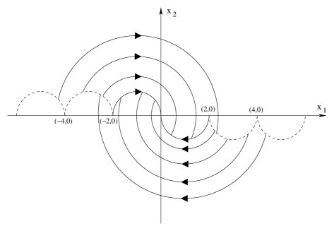
Example 3.1. Let $x\in\mathbb{R}$ and $u\in[-1,1]$. Consider the control system

$$\ddot{x}+x=u$$

and the problem of reaching the origin in minimum time. If we define $x_{1}=x$ and $x_{2}=\dot{x}$ we obtain the following first-order system:

$$\left\{\begin{array}[]{l}\dot{x}_{1}=x_{2}\\ \dot{x}_{2}=-x_{1}+u.\end{array}\right.$$ (3.1)

Every optimal trajectory is a bang-bang trajectory, i.e. formed by arcs corresponding to control $+1$ or $-1$. The synthesis is illustrated in Figure 1. There are some ”switching curves”:

• all semi-circles of radius $1$ contained in $\{(x_{1},x_{2}):x_{2}\leqslant 0\}$ and centered at $(2n+1,0)$, with $n\in\mathbb{N}\setminus\{0\}$;

• all semi-circles of radius $1$ contained in $\{(x_{1},x_{2}):x_{2}\geqslant 0\}$ and centered at $(-2n-1,0)$, with $n\in\mathbb{N}\setminus\{0\}$.

Optimal trajectories switch along these curves, i.e. change control from $+1$ to $-1$ or viceversa. Let $\gamma^{\pm}$ be the trajectory that switches at points $(\pm 2,0)$ (defined say on $[-\infty,0]$). Then the value function is not locally Lipschitz continuous at any point of supp $(\gamma^{\pm})$, but however it satisfies all the hypotheses of Theorem 5.1.

Figure 1: Synthesis of system (3.1).

$\hfill\blacktriangleleft$

Example 3.2. Let $\Omega=\mathbb{R}^{2}$, $f\equiv 0$, $L\equiv 1$. Consider the target:

$$S=\left\{(t,x):x\neq 0,t=\sin(1/x)\right\}\cup\left\{x=0,-1\leqslant t\leqslant 1\right\}\cup\left\{t\geqslant 1\right\}$$

and the final cost $\psi$ constantly equal to $0$. The value function for this problem is given by:

$$V(t,x)=\left\{\begin{array}[]{lrl}\sin(1/x)-t&\textrm{if}&x\neq 0,t\leqslant\sin(1/x)\\ 1-t&\textrm{if}&x\neq 0,\sin(1/x)<t<1\\ 0&\textrm{if}&t\geqslant 1\\ -1-t&\textrm{if}&x=0,t\leqslant-1\\ 0&\textrm{if}&x=0,-1<t<1.\end{array}\right.$$

This function satisfies all the hypotheses of Theorem 5.1 and clearly it is not continuous. Moreover it is differentiable outside a countably $\mathcal{H}^{n}$-rectifiable set $A$, which is not a locally finite union of regular manifolds. $\hfill\blacktriangleleft$

Example 3.3. (Fuller phenomenon). Let us consider the system

$$\left\{\begin{array}[]{l}\dot{x}_{1}=x_{2}\\ \dot{x}_{2}=u\end{array}\right.$$

with

Figure 2: Synthesis of Fuller phenomenon.

$\left|u\right|\leqslant 1$, $\Omega=\mathbb{R}\times\mathbb{R}^{2}$, $S=\mathbb{R}\times\{0\}$, $\psi\equiv 0$, $L(t,x_{1},x_{2},u)=x_{1}^{2}$. This problem is well-known in the literature, see for example [20]. Every optimal trajectory is composed by an infinite number of bang-bang arcs, while the time for reaching the origin of $\mathbb{R}^{2}$ is finite. There are two switching curves $\zeta^{+}$ and $\zeta^{-}$ which separate $\mathbb{R}^{2}$ into two regions $Z^{+}$ and $Z^{-}$ where the optimal trajectory uses respectively the control $u=+1$ and $u=-1$, see Figure 2. The value function of this problem satisfies all the hypotheses of Theorem 5.1. $\hfill\blacktriangleleft$

4. Some useful results.

We start by recalling without proofs some classical results about ODEs.

Proposition 4.1

(Local existence and uniqueness of the trajectory). Assume (A-1)-(A-4). Fixed $u\in\mathcal{U}$ and $(t_{0},x_{0})\in\Omega$, there exist $\delta>0$ and a unique absolutely continuous function $x(\cdot;u,t_{0},x_{0}):[t_{0},t_{0}+\delta]\to\mathbb{R}^{n}$ solution to (2.1).

Proposition 4.2

(Continuous dependence by data). Assume (A-1)-(A-4). Let $(t_{0},x_{0})\in\Omega$, $(t_{0},x_{n})\in\Omega$ for every $n\in\mathbb{N}$ and $u\in\mathcal{U}$, $u_{n}\in\mathcal{U}$ for every $n\in\mathbb{N}$. Let us suppose that there exists a time $T>t_{0}$ such that $x(\cdot;u,t_{0},x_{0})$ and $x(\cdot;u_{n},t_{0},x_{n})$ are defined in $[t_{0},T]$. If $x_{n}\to x_{0}$ and $u_{n}\to u$ in the strong topology of $L^{p}([t_{0},T];U)$ as $n\to+\infty$, then $x(\cdot;u_{n},t_{0},x_{n})\to x(\cdot;u,t_{0},x_{0})$ uniformly in $[t_{0},T]$ as $n\to+\infty$.

Now, we present two technical lemmas used to prove the theorems of the next sections.

Lemma 4.1

Fix an element $\omega\in U$, $t^{\prime}<t^{\prime\prime}$ and $x\in\mathbb{R}^{n}$ with $(t^{\prime\prime},x)\in\Omega$. Assume that there exists $\mathcal{W}$, an open neighborhood of $x$ in $\mathbb{R}^{n}$, such that $\zeta^{y}(\cdot)$, the solution to $\dot{\zeta}^{y}(t)=f(t,\zeta^{y}(t),\omega)$ with $\zeta^{y}(t^{\prime\prime})=y$, is defined on $[t^{\prime},t^{\prime\prime}]$ for any $y\in\mathcal{W}$ and $(t,\zeta^{y}(t))\in\Omega\,\,\,\,\forall t\in[t^{\prime},t^{\prime\prime}]$. Let $A$ be a countable $\mathcal{H}^{n}$-rectifiable set.
Then for a.e. $y\in\mathcal{W}$ the set $B^{y}:=\left\{t\in[t^{\prime},t^{\prime\prime}]:(t,\zeta^{y}(t))\in A\right\}$ is finite or countable.

This lemma is a slight generalization of a result proved in Theorem 2.14 of [18], since here we consider the trajectory coupled with time.

Proof. We can write $A=A_{1}\cup A_{2}$, where $A_{1}=\cup_{j}M_{j}$ and $\{M_{j}\}_{j\in J}$ is a finite or countable family of connected submanifolds of $\mathbb{R}^{n+1}$ of codimension $d_{j}>0$, and $\mathcal{H}^{n}(A_{2})=0$. After replacing each $M_{j}$ by a finite or countable family of open submanifolds of $M_{j}$, we may assume that the $M_{j}$ are embedded. Define $\widetilde{\mathcal{W}}:=]t^{\prime},t^{\prime\prime}[\times\mathcal{W}$ and let $\Phi$ be the map $\widetilde{\mathcal{W}}\ni(t,y)\mapsto(t,\zeta^{y}(t))\in\Omega$. The Jacobian of $\Phi$ is

$${\bf J}\Phi\,=\,\left(\!\begin{array}[]{l|c}1&0\,\,\cdots\cdots\,\,0\\ \hline\cr{\bf b}&\begin{matrix}\,&&\,\\[0.1pt] &{\bf V}^{\zeta}(t;t^{\prime},{\bf Id})&\\ &&\end{matrix}\end{array}\right)\!$$ (4.1)

where ${\bf b}$ is the column vector $f(t,\zeta^{y}(t),\omega)$ and ${\bf V}^{\zeta}(t;t^{\prime},{\bf Id})$ is the fundamental matrix solution to the linear system

$$\dot{v}(t)=-D_{x}f(t,\zeta^{y}(-t+t^{\prime}+t^{\prime\prime}),w)\cdot v(t)$$ (4.2)

such that ${\bf V}^{\zeta}(t^{\prime};t^{\prime},{\bf Id})={\bf Id}$. So the determinant of ${\bf J}\Phi$ is equal to the determinant of ${\bf V}^{\zeta}(t;t^{\prime},{\bf Id})$, which is equal to $exp\int_{t^{\prime}}^{t}tr(-D_{x}f(s,\zeta^{y}(-s+t^{\prime}+t^{\prime\prime}),\omega))ds$, by Liouville’s theorem (see [13]). In particular $det({\bf J}\Phi)$ is strictly positive for any $t\in[t^{\prime},t^{\prime\prime}]$. Moreover, by (A-4) $tr(-D_{x}f)$ is bounded on compact sets and then there exist $c>0$, $C>0$ such that $0<c\leqslant det({\bf J}\Phi)\leqslant C$.
So $\Phi$ is a Lipschitz diffeomorphism. In particular we have $\mathcal{H}^{n}(\Phi^{-1}(A_{2}))=0$. Now for each $j$ consider $\widetilde{M}_{j}:=\Phi^{-1}(M_{j})$. It is an embedded submanifold of codimension $d_{j}>0$. Let $\Pi:\widetilde{\mathcal{W}}\to\mathcal{W}$ be the canonical projection. Consider the set $S_{j}$ consisting of the points $s\in\widetilde{M}_{j}$ such that $\Pi{\hbox{\lower 2.5pt\hbox{$|$}}}_{\widetilde{M}_{j}}$ is not regular. Thus, by Sard’s theorem, $\mathcal{L}^{n}(\Pi(S_{j}))=0$. Moreover $\mathcal{H}^{n}(\Pi(\Phi^{-1}(A_{2})))=0$. So the set $\mathcal{B}:=\Pi(\Phi^{-1}(A_{2}))\cup(\bigcup_{j}\Pi(S_{j}))$ has Lebesgue measure $0$ in $\mathbb{R}^{n}$.
Let $y\in\mathcal{W}\setminus\mathcal{B}$. Then $(t,\zeta^{y}(t))\not\in A_{2}$ if $t^{\prime}<t<t^{\prime\prime}$. To obtain the thesis, it is sufficient to show that, for each $j$, the set $E_{j}=\left\{t\in]t^{\prime},t^{\prime\prime}[:(t,\zeta^{y}(t))\in M_{j}\right\}$ is at most countable. Fix $j$ and suppose $t\in E_{j}$. $\widetilde{M}_{j}$ has codimension $d_{j}>0$, so the dimension $\nu_{j}$ of $\widetilde{M}_{j}$ is less or equal to $n$. Since $y\not\in\mathcal{B}$, the map $d\Pi(t,y):T_{(t,y)}\widetilde{M}_{j}\to\mathbb{R}^{n}$ is onto, thus $\nu_{j}=n$ and $d\Pi(t,y)$ is injective. Obviously $d\Pi(t,y)(\frac{\partial}{\partial t})=0$, so $\frac{\partial}{\partial t}\not\in T_{(t,y)}\widetilde{M}_{j}$ and, consequently, $(\tilde{t},y)\not\in\widetilde{M}_{j}$ if $0<\left|\tilde{t}-t\right|\leqslant\varepsilon$ for $\varepsilon>0$ sufficiently small. Therefore $t$ is an isolated point of $E_{j}$ and so the lemma is proved. $\hfill\square$

Lemma 4.2

Let $g$ be a real-valued function on a compact interval $[a,b]$. Assume that there exists a finite or countable subset $E$ of $[a,b]$ with the following properties:

1. $\liminf_{h\downarrow 0}\frac{g(x+h)-g(x)}{h}\geqslant 0$ for all $x\in[a,b[\setminus E$,

2. $\liminf_{h\downarrow 0}g(x+h)\geqslant g(x)$ for all $x\in[a,b[$,

3. $\liminf_{h\downarrow 0}g(x-h)\leqslant g(x)$ for all $x\in]a,b]$.

Then $g(b)\geqslant g(a)$.

For a proof of this lemma see [18, Lemma B.1].

5. Problem with finite time.

We indicate with $\partial Q$ the topological boundary of an arbitrary $Q\subseteq\mathbb{R}\times\mathbb{R}^{n}$. Before stating the theorem we need the following definition

Definition 5.1

Suppose that we have a time-varying Lipschitz-continuous vector field $X$ on $\mathbb{R}^{n}$ and $W:\Omega\to\mathbb{R}\cup\{\pm\infty\}$. We say that $W$ has the no downward jumps property (NDJ) along $X$ if for any $[a,b]\ni t\mapsto\gamma(t)$, solution to $\dot{\gamma}(t)=X(t,\gamma(t))$ such that $(t,\gamma(t))\in\Omega$ $\forall t\in[a,b]$, we have $\liminf_{h\downarrow 0}W(t-h,\gamma(t-h))\leqslant W(t,\gamma(t))$, whenever $t\in]a,b]$.

Theorem 5.1

Suppose (A-1)-(A-5) hold. Let $Q\subseteq\Omega$ be an open subset containing $S$. Let $W:\overline{Q}\to\mathbb{R}$ be a lower semicontinuous function such that:

1. $W$ has the NDJ property along every time-varying vector field of the type $f(t,x,u)$ with $u\in U$ fixed and for each $t$

   $${\textrm{ess-liminf}}_{y\to x}W(t,y)\leqslant W(t,x).$$

2. $W\leqslant\psi$ on $S$.

3. At every point $(t,x)\in\partial Q$ one has

   $$W(t,x)=\sup_{(s,y)\in Q}W(s,y).$$

4. There exists a countably $\mathcal{H}^{n}$-rectifiable set $A\subseteq\Omega$ such that $W$ is differentiable on $Q\setminus A$ and satisfies

   $$W_{s}(s,y)+\inf_{\omega\in U}\left\{W_{y}(s,y)\cdot f(s,y,\omega)+L(s,y,\omega)\right\}\geqslant 0\quad\textrm{on }Q\setminus A.$$

5. $L\geqslant 0$.

Then $W\leqslant V$ on $Q$. If $Q=\Omega$ we can drop hypotheses iii) and v).

Proof. Suppose by contradiction that there exists $(t_{0},x_{0})\in Q$ such that $W(t_{0},x_{0})>V(t_{0},x_{0})$. In particular $V(t_{0},x_{0})<+\infty$. First of all, let us consider the case $V(t_{0},x_{0})>-\infty$. So we can find $\varepsilon>0$, $\delta>0$ such that

$$V(t_{0},x_{0})\leqslant W(t_{0},x_{0})-2\varepsilon$$ (5.1)

and, by the lower semicontinuity of $W$,

$$\left|x-x_{0}\right|<\delta\quad\Rightarrow\quad W(t_{0},x)>V(t_{0},x_{0})+\varepsilon.$$ (5.2)

We can find $u^{\ast}\in\mathcal{U}$ such that $x^{\ast}(\cdot):=x(\cdot;u^{\ast},t_{0},x_{0})$ satisfies $(T,x^{\ast}(T))\in S$ and

$$\int_{t_{0}}^{T}L(s,x^{\ast}(s),u^{\ast}(s))ds+\psi(T,x^{\ast}(T))\leqslant V(t_{0},x_{0})+\frac{\varepsilon}{2}\,\,.$$ (5.3)

Moreover, for every $l\in\mathbb{N}$ there exists $u_{l}\in\mathcal{U}$ such that $\|u_{l}-u^{\ast}\|_{L^{p}([t_{0},T])}\leqslant\frac{1}{l}$, $u_{l}$ piecewise constant and left continuous. By [6, Théorèm IV.9], there exists a subsequence of $(u_{l})_{l}$, denoted again by $(u_{l})_{l}$, and a function $h\in L^{p}([t_{0},T])$ such that $|u_{l}|\leqslant h$ a.e. and $u_{l}$ converges to $u^{\ast}$ a.e. as $l\to+\infty$. Hence, if we denote by $x_{l}(\cdot)$ the trajectory $x(\cdot;u_{l},T,x^{\ast}(T))$, for $l$ sufficiently big, we have (see Proposition 4.2),

$$\left|x_{l}(t)-x^{\ast}(t)\right|<\frac{\delta}{2}\quad\quad\forall t\in[t_{0},T]$$ (5.4)

and

$$\left|\int_{t_{0}}^{T}[L(s,x_{l}(s),u_{l}(s))-L(s,x^{\ast}(s),u^{\ast}(s))]ds\right|\leqslant\frac{\varepsilon}{2}.$$ (5.5)

Fix $l$ such that (5.4) and (5.5) hold and an interval $]t^{\prime},t^{\prime\prime}]$ such that $u_{l}(t)\equiv\omega$ on $]t^{\prime},t^{\prime\prime}]$. Suppose that $(t,x_{l}(t))\in Q\,\,\,\forall t\in[t^{\prime},t^{\prime\prime}]$. Let $\zeta^{y}(t)$ be the trajectory associated to the constant control $\omega$ such that $\zeta^{y}(t^{\prime\prime})=y$. By the fact that $d(\partial Q,\{(t,x_{l}(t)):t\in[t^{\prime},t^{\prime\prime}]\})>0$, we can find an open neighborhood $\mathcal{W}$ of $x_{l}(t^{\prime\prime})$ in $\mathbb{R}^{n}$ such that $(t^{\prime\prime},y)\in Q\,\,\,\forall y\in\mathcal{W}$ and $\left\{(t,\zeta^{y}(t)):t\in[t^{\prime},t^{\prime\prime}]\right\}\subseteq Q\,\,\,\forall y\in\mathcal{W}$. By Lemma 4.1, we have that for a.e. $y\in\mathcal{W}$ the set $B^{y}:=\left\{t\in[t^{\prime},t^{\prime\prime}]:(t,\zeta^{y}(t))\in A\right\}$ is at most countable.
Therefore,since for every fixed $t$ $\textrm{ess-liminf}_{y\to x}W(t,y)\leqslant W(t,x)$, then for every $\delta_{j}\to 0$, $\delta_{j}>0$ there exists a sequence $(y_{j}^{l})_{j}\in\mathbb{N}$ such that $y_{j}^{l}\to x_{l}(t^{\prime\prime})$, $W(t^{\prime\prime},y_{j}^{l})\leqslant W(t^{\prime\prime},x_{l}(t^{\prime\prime}))+\delta_{j}$ and $B^{y_{j}^{l}}$ is at most countable. Consider the following function defined on $[t^{\prime},t^{\prime\prime}]$:

$$\varphi^{l}_{j}(t):=W(t,\zeta^{y_{j}^{l}}(t))+\int_{t^{\prime}}^{t}L(s,\zeta^{y_{j}^{l}}(s),\omega)ds.$$

By the choice of $y_{j}^{l}$ and the hypotheses $\ref{i4})$, $\varphi_{j}^{l}$ is differentiable a.e. with a nonnegative derivative. By the lower semicontinuity of $W$ and the NDJ condition, it follows that $\varphi^{l}_{j}$ verifies the hypotheses of Lemma 4.2 and so $\varphi^{l}_{j}(t^{\prime})\leqslant\varphi^{l}_{j}(t^{\prime\prime})$. Thus

$$W(t^{\prime},\zeta^{y_{j}^{l}}(t^{\prime}))\leqslant W(t^{\prime\prime},\zeta^{y_{j}^{l}}(t^{\prime\prime}))+\int_{t^{\prime}}^{t^{\prime\prime}}L(s,\zeta^{y_{j}^{l}}(s),\omega)ds.$$ (5.6)

Now, using the fact that $\zeta^{y_{j}^{l}}(t^{\prime\prime})=y_{j}^{l}$ we obtain

$$W(t^{\prime},\zeta^{y_{j}^{l}}(t^{\prime})) \leqslant W(t^{\prime\prime},y_{j}^{l})+\int_{t^{\prime}}^{t^{\prime\prime}}L(s,\zeta^{y_{j}^{l}}(s),\omega)ds$$ (5.7)

$$\leqslant W(t^{\prime\prime},x_{l}(t^{\prime\prime}))+\delta_{j}+\int_{t^{\prime}}^{t^{\prime\prime}}L(s,\zeta^{y_{j}^{l}}(s),\omega)ds.$$

By Proposition 4.2, $\zeta^{y_{j}^{l}}(\cdot)\to x_{l}(\cdot)$ as $j\to+\infty$ and so by the Lebesgue theorem and the lower semicontinuity of $W$, passing to the limit as $j\to+\infty$ we obtain:

$$W(t^{\prime},x_{l}(t^{\prime}))\leqslant W(t^{\prime\prime},x_{l}(t^{\prime\prime}))+\int_{t^{\prime}}^{t^{\prime\prime}}L(s,x_{l}(s),\omega)ds.$$ (5.8)

First consider the case $\left\{(t,x_{l}(t)):t\in[t_{0},T]\right\}\subseteq Q$. Summing (5.8) over each interval on which $u_{l}$ is constant we have

$$W(t_{0},x_{l}(t_{0}))\leqslant W(T,x_{l}(T))+\int_{t_{0}}^{T}L(s,x_{l}(s),u_{l}(s))ds.$$ (5.9)

Now, $x_{l}(T)=x^{\ast}(T)$ by definition and so, using (5.2-5.5) and ii)

$$W(t_{0},x_{l}(t_{0})) \leqslant W(T,x^{\ast}(T))+\int_{t_{0}}^{T}L(s,x_{l}(s),u_{l}(s))ds$$

$$\leqslant \psi(T,x^{\ast}(T))+\int_{t_{0}}^{T}L(s,x_{l}(s),u_{l}(s))ds$$

$$\leqslant V(t_{0},x_{0})+\frac{\varepsilon}{2}-\int_{t_{0}}^{T}L(s,x^{\ast}(s),u^{\ast}(s))ds$$

$$+\int_{t_{0}}^{T}L(s,x_{l}(s),u_{l}(s))ds$$

$$\leqslant V(t_{0},x_{0})+\varepsilon<W(t_{0},x_{l}(t_{0})).$$

This is a contradiction.
Suppose now $\left\{(t,x_{l}(t)):t\in[t_{0},T]\right\}\not\subseteq Q$. Define

$$\hat{\tau}:=\inf\left\{t\leqslant T:(s,x_{l}(s))\in Q\quad\forall s\in[t,T]\right\}.$$ (5.10)

In particular $(\hat{\tau},x_{l}(\hat{\tau}))\in\partial Q$. Using the same argument to pass from (5.8) to (5.9), we obtain that for every $\tau>\hat{\tau}$

$$W(\tau,x_{l}(\tau))\leqslant W(T,x^{\ast}(T))+\int_{\tau}^{T}L(s,x_{l}(s),u_{l}(s))ds$$ (5.11)

and so, using ii) and (5.3)

$$W(\tau,x_{l}(\tau)) \leqslant \psi(T,x^{\ast}(T))+\int_{\tau}^{T}L(s,x_{l}(s),u_{l}(s))ds$$ (5.12)

$$\leqslant V(t_{0},x_{0})+\frac{\varepsilon}{2}-\int_{t_{0}}^{T}L(s,x^{\ast}(s),u^{\ast}(s))ds$$

$$+\int_{\tau}^{T}L(s,x_{l}(s),u_{l}(s))ds.$$

Using (5.1), (5.5) and v), we obtain for all $\tau>\hat{\tau}$

$$W(\tau,x_{l}(\tau))\leqslant V(t_{0},x_{0})+\varepsilon\leqslant W(t_{0},x_{0})-\varepsilon.$$ (5.13)

Passing to the liminf as $\tau\to\hat{\tau}$ and using the lower semicontinuity of $W$, we conclude

$$W(\hat{\tau},x_{l}(\hat{\tau}))\leqslant W(t_{0},x_{0})-\varepsilon$$ (5.14)

and so by $\ref{i3})$

$$W(t_{0},x_{0})\leqslant\sup_{(t,x)\in Q}W(t,x)\leqslant W(t_{0},x_{0})-\varepsilon$$ (5.15)

which is a contradiction.

Now, we have to treat the case $V(t_{0},x_{0})=-\infty$. Since $W(t_{0},x_{0})>-\infty$ and $W$ is lower semicontinuous, we may find two constants $M>1$ and $\delta>0$ such that:

$$W(t_{0},x)>-M$$

for every $x$ so that $\left|x-x_{0}\right|<\delta$. Moreover we can find $u^{\ast}\in\mathcal{U}$ such that $x^{\ast}(\cdot):=x(\cdot;u^{\ast},t_{0},x_{0})$ satisfies $(T,x^{\ast}(T))\in S$ and

$$\int_{t_{0}}^{T}L(s,x^{\ast}(s),u^{\ast}(s))ds+\psi(T,x^{\ast}(T))\leqslant-2M.$$

With the same arguments of the first part of the proof we may find a control $u_{l}\in\mathcal{U}$ piecewise constant and left continuous such that, if $x_{l}(\cdot)$ is the trajectory $x(\cdot;u_{l},T,x^{\ast}(T))$,

$$\left|x_{l}(t)-x^{\ast}(t)\right|<\frac{\delta}{2}\quad\forall t\in[t_{0},T]$$

and

$$\left|\int_{t_{0}}^{T}[L(s,x_{l}(s),u_{l}(s))-L(s,x^{\ast}(s),u^{\ast}(s))]ds\right|\leqslant 1.$$

Repeating the same calculations as before, we obtain that

$$-M \leqslant W(T,x^{\ast}(T))+\int_{t_{0}}^{T}L(s,x_{l}(s),u_{l}(s))ds$$

$$\leqslant \psi(T,x^{\ast}(T))+\int_{t_{0}}^{T}L(s,x^{\ast}(s),u^{\ast}(s))ds+1$$

$$\leqslant -2M+1$$

which gives $M\leqslant 1$, a contradiction.

This concludes the proof of the theorem. $\hfill\square$

Corollary 5.1

Let us suppose that $W$ satisfies all the hypotheses of the previous theorem. If moreover $W\geqslant V$ then $W=V$.

Remark 5.1. If $W$ is produced by a synthesis procedure, the inequality $W\geqslant V$ always holds and so if $W$ satisfies all the hypotheses of Theorem 5.1 then $W$ coincides with the value function. $\hfill\lhd$

Using the same techniques of the previous theorem, we can prove a corollary for value functions generated by approximated syntheses, and give a bound of the error thus produced.

Corollary 5.2

Suppose (A1)-(A5) hold. Let $Q\subseteq\Omega$ be an open subset containing $S$. Let $W:\overline{Q}\to\mathbb{R}$ be a lower semicontinuous function verifying the NDJ property along every time-varying vector field of the type $f(t,x,u)$ with $u\in U$ fixed. Moreover we assume that, for each $t$, ${\textrm{ess-liminf}}_{y\to x}W(t,y)\leqslant W(t,x)$ and that there exist $\varepsilon>0$ and $g\in L^{1}(\mathbb{R})$, $g\geqslant 0$, such that:

1. $W\leqslant\psi+\varepsilon$ on $S$.

2. At every point $(t,x)\in\partial Q$ one has

   $$W(t,x)=\sup_{(s,y)\in Q}W(s,y).$$

3. There exists a countably $\mathcal{H}^{n}$-rectifiable set $A\subseteq\Omega$ such that $W$ is differentiable on $Q\setminus A$ and satisfies

   $$W_{s}(s,y)+\inf_{\omega\in U}\left\{W_{y}(s,y)\cdot f(s,y,\omega)+L(s,y,\omega)\right\}\geqslant-\varepsilon g(s)\quad\textrm{on }Q\setminus A.$$

4. $L\geqslant-\varepsilon g$.

Then $W\leqslant V+\varepsilon(1+\|g\|_{1})$ on $Q$.

Proof. Note that $L(t,x,u)+\varepsilon g(t)\geqslant 0$ and so

$$W(t_{0},x_{0}) \leqslant \!\!\!\!\!\!\!\!\!\!\!\!\inf_{\begin{subarray}{c}u\in\mathcal{U}\vspace{3pt}\\ (T,x(T;u,t_{0},x_{0}))\in S\end{subarray}}\!\!\!\left\{\int_{t_{0}}^{T}\!\!\!\!\!\!L(s,x(s;u,t_{0},x_{0}),u(s))ds\!+\!\psi(T,x(T;u,t_{0},x_{0}))\right\}$$

$$\leqslant V(t_{0},x_{0})+\varepsilon(1+\|g\|_{L^{1}}).$$

$\hfill\square$

Remark 5.2. Notice that the value function of an optimal control problem has the NDJ property along every possible direction as a consequence of the Dynamic Programming Principle. Indeed, for every $(t,y)\in\Omega\setminus S$ and for every admissible control $u\in\mathcal{U}$ (in particular for every control $\omega\chi_{I}$, where $\omega\in U$ and $I$ bounded interval), the function

$$h\mapsto\int_{t}^{t+h}L(s,x(s;u,t,y),u(s))ds+V(t+h,x(t+h;u,t,y))$$

is non decreasing for $h\in[0,\delta]$ and $\delta$ small enough.

Instead, the hypothesis

$$\textrm{ess-liminf}_{y\to x}W(t,y)\leqslant W(t,x)$$

for each $t$ fixed, says that, for every $\varepsilon>0$ there exists a subset $V\subseteq\{y\in\mathbb{R}^{n}:\left|y-x\right|\leqslant\varepsilon\}$ of strictly positive Lebesgue measure such that

$$\inf_{y\in V}W(t,y)\leqslant W(t,x).$$

So, if we consider a set $V_{1}\subseteq\mathbb{R}^{n}$ of zero Lebesgue measure with $x$ as a cluster point, the set $V\setminus V_{1}$ has a strictly positive Lebesgue measure. In the proof of Theorem 5.1 this fact is used to avoid the points $y$ for which $B^{y}$ is not countable. Moreover this hypothesis, coupled with the lower semicontinuity of $W$, gives the following:

• for each $t$,

  $$W(t,x)=\liminf_{y\to x}W(t,y)=\textrm{ess-liminf}_{y\to x}W(t,y).$$

$\hfill\lhd$

Remark 5.3. Hypothesis iii) of Theorem 5.1 says that, in the case $Q\neq\Omega$, the boundary of $Q$ must be a level set of the function $W$. We can relax the same hypothesis in the following way:

• At every point $(t,x)\in\partial Q$ one has

  $$\liminf_{\begin{subarray}{c}\tau\to t,y\to x\\ (\tau,y)\in Q\end{subarray}}W(\tau,y)\geqslant\sup_{(s,y)\in Q}W(s,y)$$

and the conclusion of the theorem remains valid. Moreover if we define with $R(t,x)$ the set of point reachable with an admissible control from $(t,x)$, the previous condition can be replaced by

$$\inf_{(s,y)\in R(t,x)\cap\partial Q}W(s,y)\geqslant W(t,x)$$

and the conclusion still holds. $\hfill\lhd$

The hypotheses of the positiveness of $L$ is almost optimal as the next example shows. However, the Lagrangian $L$ may be negative on some region if trajectories can not stay for too long in such a region and one can relax the assumption v) as shown in Remark 5.4.
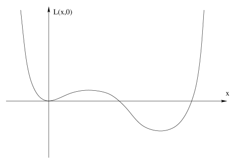
Example 5.1.

Figure 3: $L(x,0)$ of Example 5.1.

Consider the system $\dot{x}=u$, $U=[-1,1]\,$ and $\,\mathcal{U}=L^{1}(\mathbb{R};U)$, $\Omega=\mathbb{R}^{2}$, $S=\mathbb{R}\times\{0\}$, $Q=\mathbb{R}\times]-1,1[$ with the Lagrangian $L(t,x,u)=u^{2}+x^{4}-6x^{3}+7x^{2}$ (see Figure 3) and $\psi\equiv 0$ on $S$. Since the Lagrangian is negative in a region where the system can stay for an arbitrary interval of times, clearly the value function for this problem is equal to $-\infty$. If $W\equiv C$ on $\overline{Q}$ with $C$ negative constant, then $W$ verifies all the hypotheses of the Theorem 5.1, but v). In fact i), ii), iii) are obvious, while iv) holds because $L$ is positive on $Q$ and $W$ is differentiable on $Q$. So there exist infinitely many functions $W$ defined on $\overline{Q}$ verifying the hypotheses of Theorem 5.1, but v), which are not lower or equal to the value function $V$. $\hfill\blacktriangleleft$

Remark 5.4. If one wants to eliminate hypothesis v) from the previous theorem, one may assume one of the following conditions:

1. Fix $\varepsilon>0$ and $(\bar{t},\bar{x})\in Q$. We call $x_{\varepsilon}:[\bar{t},T]\to\mathbb{R}^{n}$ an $\varepsilon$-quasi optimal trajectory ($\varepsilon$-q.o.t.) for $(\bar{t},\bar{x})$ if:

   1. $\exists\,u_{\varepsilon}\in\mathcal{U}$ such that $\dot{x}_{\varepsilon}(s)=f(s,x_{\varepsilon}(s),u_{\varepsilon}(s))$ for a.e. $s\in[\bar{t},T]$,

   2. $x_{\varepsilon}(\bar{t})=\bar{x}$,

   3. $(T,x_{\varepsilon}(T))\in S$,

   4. $V(\bar{t},\bar{x})+\varepsilon\geqslant\int_{\bar{t}}^{T}L(s,x_{\varepsilon}(s),u_{\varepsilon}(s))ds+\psi(T,x_{\varepsilon}(T))$.

   Now define $Q_{1}$ as the set of point $(\bar{t},\bar{x})\in Q$ such that, for every $\varepsilon>0$, there exists $x_{\varepsilon}$, an $\varepsilon$-q.o.t. for $(\bar{t},\bar{x})$, satisfying $(s,x_{\varepsilon}(s))\in Q$ for any $s\in[\bar{t},T]$. What we need is that $L\geqslant 0$ in $\Omega\setminus Q_{1}$. In fact, under this assumption, we may suppose that $(s,x(s))\in\Omega\setminus Q_{1}$ for every $s\in[t_{0},\hat{\tau}[$, where $x$ is the trajectory defined in the proof of Theorem 5.1 and the time $\hat{\tau}$ is defined in (5.10). So the integral $\int_{t_{0}}^{\hat{\tau}}L(s,x(s),u(s))ds$ is positive. Otherwise we can assume $Q_{1}=Q$.

2. We can also use an hypothesis similar to one given in [14]. For any $(\bar{t},\bar{x})\in\Omega$ and $u\in\mathcal{U}$, let $x_{\bar{t},\bar{x}}(\cdot;u):=x(\cdot;u,\bar{t},\bar{x})$ be the solution to (2.1) associated to the control $u$. Consider the set $P$ consisting of those points $(\bar{t},\bar{x})$ of $Q$ such that

   $$\int_{\bar{t}}^{T}L(s,x_{\bar{t},\bar{x}}(s;u),u(s))ds\geqslant 0\qquad\forall T>t\quad\forall u\in\mathcal{U}.$$

   We have to suppose that, if $(\bar{t},\bar{x})\in Q\setminus[P\cup S]$, there exist a bounded and open set $B$, $(\bar{t},\bar{x})\in B\subseteq Q$, $B\cap S=\emptyset$, so that $\partial B\subseteq Q$, and a positive number $M$ strictly less than

   $$\inf_{u\in\mathcal{U}}\left\{T>0:d((\bar{t}+T,x_{\bar{t},\bar{x}}(\bar{t}+T;u)),\partial B)\leqslant d((\bar{t},\bar{x}),\partial B)/2\right\}$$

   such that, for all $u\in\mathcal{U}$, $(M+\bar{t},x_{\bar{t},\bar{x}}(M+\bar{t};u))\in Q\cap P$ and

   $$\int_{\bar{t}}^{\bar{t}+M}L(s,x_{\bar{t},\bar{x}}(s),u(s))ds\geqslant 0,$$

   and this allow to conclude the proof of Theorem 5.1 without using $L\geqslant 0$ on the whole space.

$\hfill\lhd$

Example 5.2. Consider the system $\dot{x}=u$, $U=[-1,1]$, $\mathcal{U}=L^{1}(\mathbb{R};U)$, $\Omega=\mathbb{R}^{+}\times\mathbb{R}$, $S=\mathbb{R}^{+}\times\{0\}$, $Q=\mathbb{R}^{+}\times]-1,1[$, $\psi=0$ on $S$ and the Lagrangian defined by

$$L(t,x,u):=\left\{\begin{array}[]{lrl}u^{2}+x^{2}&\textrm{if}&x\leqslant 1\\ (u^{2}+1)(2-x)+(x-1)(u^{2}+Ct)&\textrm{if}&1<x<2\\ u^{2}+x^{2}-6x+8+Ct&\textrm{if}&x\geqslant 2\end{array}\right.$$

It is clear that this Lagrangian, for $C$ sufficiently big, satisfies the conditions a) and b) of the previous remark, even if it is not positive outside $Q$. $\hfill\blacktriangleleft$

Remark 5.5. We can relax hypotheses iii) and v) with the following:

iii’)

the boundary $\partial Q$ is a level set of $W$;

v’)

$L\geqslant 0$ on $\Omega\setminus Q$.

With these hypotheses, we can obtain an inequality of type (5.8) for each interval where the couple time-trajectory is in $Q$ and then, using $iii^{\prime})$, $v^{\prime})$, the lower semicontinuity of $W$ and the NDJ property we can obtain (5.9). $\hfill\lhd$

6. Problem with infinite time.

In this section we consider the control system (2.1) and assume that (A-1)-(A-5) hold with $0\leq C_{R}\leq C$ for some $C>0$ and every $R>0$. Moreover we suppose that the target $S$ is a closed subset of $\mathbb{R}\times\mathbb{R}^{n}$ which satisfies the structural property:

$(\ast)$

For any $T>0$, there exists $(t,x)\in S$ with $t\geqslant T$.

Let $S_{1}$ be an open neighborhood of $S$ contained in $\Omega$. Assume that the final cost $\psi$ is defined on $S_{1}$ and, if $d((t,x(t;u,t_{0},x_{0})),S)\to 0$ as $t\to+\infty$, then the trajectory $x(\cdot;u,t_{0},x_{0})$ is definitively in $S_{1}$, that is:

$(\ast\ast)$

$\!\!\!\exists\,T>t$ such that $(s,x(s;u,t_{0},x_{0}))\in S_{1}$ for all $s\geqslant T$.

Define the value function:

$$V(t_{0},x_{0}):=\!\!\!\!\!\!\!\!\!\!\!\!\!\!\!\inf_{\begin{subarray}{c}u\in\mathcal{U}\\[5.0pt] d((t,x(t;u,t_{0},x_{0})),S)\to 0\\ \text{as }t\to+\infty\end{subarray}}\!\!\!\!\!\!\!\!\!\!\!\!\!\left\{\!\int_{t_{0}}^{+\infty}\!\!\!\!\!\!\!\!\!\!\!L(s,x(s;u,t_{0},x_{0}),u(s))ds\!+\!\limsup_{t\to+\infty}\psi(t,x(t;u,t_{0},x_{0}))\right\}$$ (6.1)

In other words, we consider only the trajectories that approach the target $S$ in infinite time. Notice that this condition does not imply that $(T,x(T))\not\in S$ for any $T\geqslant t_{0}$.

Remark 6.1. The introduction of an open neighborhood of the target $S$ is due to a technical reason and precisely to the fact that it is necessary to compare the candidate value function to the final cost near the target. Notice that in the following theorem the set $Q$ must contain $S_{1}$. For example we consider $\Omega=\mathbb{R}^{+}\times\mathbb{R}$, $S=\mathbb{R}^{+}\times\{0\}$, $Q=\{(t,x):t>0,x<1/t\}$ and $S_{1}=\{(t,x):t>0,x<3/t\}$. If $(t,2/t)$, with $t>0$, is a trajectory, then it is definitely in $S_{1}$, but it is never in $Q$. $\hfill\lhd$

Theorem 6.1

Let $Q\subseteq\Omega$ be an open subset containing $S_{1}$. Let $W:\overline{Q}\to\mathbb{R}$ be a lower semicontinuous function such that

1. $W$ has the NDJ property along every time-varying vector field of the type $f(t,x,u)$ with $u\in U$ fixed and for each $t$,

   $$\textrm{ess-liminf}_{y\to x}W(t,y)\leqslant W(t,x).$$

2. $W\leqslant\psi$ on $S_{1}$.

3. At every point $(t,x)\in\partial Q$ one has

   $$W(t,x)=\sup_{(s,y)\in Q}W(s,y).$$

4. There exists a countable $\mathcal{H}^{n}$-rectifiable set $A\subseteq\Omega$ such that $W$ is differentiable in $Q\setminus A$ and satisfies

   $$W_{s}(s,y)+\inf_{\omega\in U}\left\{W_{y}(s,y)\cdot f(s,y,\omega)+L(s,y,\omega)\right\}\geqslant 0\quad\textrm{in }Q\setminus A.$$

5. $L\geqslant 0$.

Then $W\leqslant V$ on $Q$. If $Q=\Omega$ we can drop hypotheses iii) and v).

Proof. Suppose by contradiction that there exists $(t_{0},x_{0})\in Q$ such that $W(t_{0},x_{0})>V(t_{0},x_{0})$. In particular $V(t_{0},x_{0})<+\infty$. First of all, let us consider the case $V(t_{0},x_{0})>-\infty$. As in the first part of the proof of Theorem 5.1, we can find $\varepsilon>0$ and $\delta>0$ such that the following holds:

$$V(t_{0},x_{0})\leqslant W(t_{0},x_{0})-2\varepsilon$$ (6.2)

$$\left|x-x_{0}\right|<\delta\quad\Rightarrow\quad W(t_{0},x)>V(t_{0},x_{0})+\frac{3\varepsilon}{2}\,\,.$$ (6.3)

We can choose $u^{\ast}\in\mathcal{U}$, with the property that the trajectory $(t,x^{\ast}(t))$ approaches the target when $t\to+\infty$, and such that

$$\int_{t_{0}}^{+\infty}L(s,x^{\ast}(s),u^{\ast}(s))ds+\limsup_{t\to+\infty}\psi(t,x^{\ast}(t))\leqslant V(t_{0},x_{0})+\frac{\varepsilon}{2}\,\,,$$ (6.4)

where $x^{\ast}(\cdot)$ is the trajectory corresponding to the control $u^{\ast}$ such that $x^{\ast}(t_{0})=x_{0}$.
Consider, now, a strictly increasing sequence of times $T_{j}>t_{0}$ converging to $+\infty$. We may suppose that $(t,x^{\ast}(t))\in Q$ for every $t\geqslant T_{1}$. Fix $j\in\mathbb{N}$. For every $l\in\mathbb{N}$, there exists $u_{j}^{l}\in\mathcal{U}$ piecewise constant and left continuous such that $\|u_{j}^{l}-u^{\ast}\|_{L^{p}([t_{0},T_{j}])}\leqslant\frac{1}{l}$. So, by [6, Théorèm IV.9], we can extract a subsequence of $(u_{j}^{l})_{l}$, denoted again with $(u_{j}^{l})_{l}$, and we can find a function $h_{j}\in L^{p}([t_{0},T_{j}])$ such that $|u_{j}^{l}|\leqslant h_{j}$ a.e. for every $l\in\mathbb{N}$ and $u_{j}^{l}\to u^{\ast}$ for a.e. $t\in[t_{0},T_{j}]$ as $l\to+\infty$. Thus denoting with $x_{j}^{l}(\cdot)$ the trajectory $x(\cdot;u_{j}^{l},T_{j},x^{\ast}(T_{j}))$, for $l$ sufficiently big we have (see Proposition 3.2)

$$\left|x_{j}^{l}(t)-x^{\ast}(t)\right|\leqslant\frac{\delta}{2}\qquad\forall t\in[t_{0},T_{j}]$$ (6.5)

and then

$$\left|\int_{t_{0}}^{T_{j}}\left[L(s,x_{j}^{l}(s),u_{j}^{l}(s))-L(s,x^{\ast}(s),u^{\ast}(s))\right]ds\right|\leqslant\frac{\varepsilon}{2}\,\,.$$ (6.6)

Now, fix $l\in\mathbb{N}$ such that (6.5) and (6.6) hold. First, let us suppose that $\{(t,x_{j}^{l}(t)):t\in[t_{0},T_{j}]\}\subseteq Q$. So, using Lemma 4.1, Lemma 4.2, the same arguments as in the proof of Theorem 5.1 and (6.6) we conclude

$$W(t_{0},x_{j}^{l}(t_{0})) \leqslant W(T_{j},x_{j}^{l}(T_{j}))+\int_{t_{0}}^{T_{j}}L(s,x_{j}^{l}(s),u_{j}^{l}(s))ds$$

$$\leqslant W(T_{j},x^{\ast}(T_{j}))+\int_{t_{0}}^{T_{j}}L(s,x^{\ast}(s),u^{\ast}(s))ds+\frac{\varepsilon}{2}\,\,.$$

Using (6.3) and (6.5) we have

$$V(t_{0},x_{0})+\frac{3\varepsilon}{2}<W(T_{j},x^{\ast}(T_{j}))+\int_{t_{0}}^{T_{j}}L(s,x^{\ast}(s),u^{\ast}(s))ds+\frac{\varepsilon}{2}\,\,.$$ (6.7)

Now consider the other case and precisely $\{(t,x_{j}^{l}(t)):t\in[t_{0},T_{j}]\}\not\subseteq Q$. Define

$$\tau_{j}^{l}:=\inf\left\{t\geqslant t_{0}:(s,x_{j}^{l}(s))\in Q\,\,\,\,\forall s\in[t,T_{j}]\right\}.$$ (6.8)

Given $\tau_{j}^{l}<t<T_{j}$

$$W(t,x_{j}^{l}(t))\leqslant W(T_{j},x_{j}^{l}(T_{j}))+\int_{t}^{T_{j}}L(s,x_{j}^{l}(s),u_{j}^{l}(s))ds.$$ (6.9)

Considering the fact that $(t,x_{j}^{l}(t))\to(\tau_{j}^{l},x_{j}^{l}(\tau_{j}^{l}))$ as $t\to\tau_{j}^{l}$, $(\tau_{j}^{l},x_{j}^{l}(\tau_{j}^{l}))\in\partial Q$ and (iii) we obtain

$$W(t_{0},x_{0})\leqslant W(T_{j},x^{\ast}(T_{j}))+\int_{\tau_{j}^{l}}^{T_{j}}L(s,x_{j}^{l}(s),u_{j}^{l}(s))ds.$$ (6.10)

We can now use the hypothesis $\ref{ii5})$, (6.3) and (6.6) in order to have

$$V(t_{0},x_{0})+\frac{3\varepsilon}{2}<W(t_{0},x_{0})\leqslant$$

$$\leqslant W(T_{j},x^{\ast}(T_{j}))+\int_{t_{0}}^{T_{j}}L(s,x^{\ast}(s),u^{\ast}(s))ds+\frac{\varepsilon}{2}\,\,.$$ (6.11)

In all cases we have that, for every $j\in\mathbb{N}$,

$$V(t_{0},x_{0})+\frac{3\varepsilon}{2}<W(T_{j},x^{\ast}(T_{j}))+\int_{t_{0}}^{T_{j}}L(s,x^{\ast}(s),u^{\ast}(s))ds+\frac{\varepsilon}{2}\,\,.$$ (6.12)

So, applying the limsup as $j\to+\infty$ we get

$$V(t_{0},x_{0})+\frac{3\varepsilon}{2} \leqslant \limsup_{j\to+\infty}W(T_{j},x^{\ast}(T_{j}))+\int_{t_{0}}^{+\infty}\!\!\!L(s,x^{\ast}(s),u^{\ast}(s))ds+\frac{\varepsilon}{2}$$

$$\leqslant \limsup_{t\to+\infty}W(t,x^{\ast}(t))+\int_{t_{0}}^{+\infty}\!\!\!L(s,x^{\ast}(s),u^{\ast}(s))ds+\frac{\varepsilon}{2}\,\,.$$

For $t$ sufficiently big, $(t,x^{\ast}(t))\in S_{1}$ and so, using (ii) and (6.4),

$$V(t_{0},x_{0})+\frac{3\varepsilon}{2} \leqslant \limsup_{t\to+\infty}\psi(t,x^{\ast}(t))+\int_{t_{0}}^{+\infty}L(s,x^{\ast}(s),u^{\ast}(s))ds+\frac{\varepsilon}{2}$$

$$\leqslant V(t_{0},x_{0})+\varepsilon$$

which implies

$$V(t_{0},x_{0})\leqslant V(t_{0},x_{0})-\frac{\varepsilon}{2}$$

which is a contradiction.

It remains the case $V(t_{0},x_{0})=-\infty$. Since $W(t_{0},x_{0})>-\infty$ and $W$ is lower semicontinuous, we may find two constants $M>1$ and $\delta>0$ such that

$$W(t_{0},x)>-M$$

for every $x$ so that $\left|x-x_{0}\right|<\delta$. Moreover we can find $u^{\ast}\in\mathcal{U}$ such that $x^{\ast}(\cdot):=x(\cdot;u^{\ast},t_{0},x_{0})$ approaches the target when $t\to+\infty$ and

$$\int_{t_{0}}^{+\infty}L(s,x^{\ast}(s),u^{\ast}(s))ds+\limsup_{t\to+\infty}\psi(t,x^{\ast}(t))\leqslant-2M.$$

Consider a strictly increasing sequence of times $T_{j}>t_{0}$ converging to $+\infty$ and repeat the previous arguments in order to find a control $u_{j}^{l}\in\mathcal{U}$ piecewise constant, left continuous and such that, if $x_{j}^{l}(\cdot):=x(\cdot;u_{j}^{l},T_{j},x^{\ast}(T_{j}))$,

$$\left|x_{j}^{l}(t)-x^{\ast}(t)\right|\leqslant\frac{\delta}{2}\quad\forall t\in[t_{0},T_{j}]$$

and

$$\left|\int_{t_{0}}^{T_{j}}[L(s,x_{j}^{l}(s),u_{j}^{l}(s))-L(s,x^{\ast}(s),u^{\ast}(s))]ds\right|\leqslant 1.$$

Proceeding as before we obtain that

$$-M \leqslant W(T_{j},x^{\ast}(T_{j}))+\int_{t_{0}}^{T_{j}}L(s,x_{j}^{l}(s),u_{j}^{l}(s))ds$$

$$\leqslant W(T_{j},x^{\ast}(T_{j}))+\int_{t_{0}}^{T_{j}}L(s,x^{\ast}(s),u^{\ast}(s))ds+1$$

for every $j\in\mathbb{N}$. Passing to the limit we have:

$$-M \leqslant \limsup_{j\to+\infty}W(T_{j},x^{\ast}(T_{j}))+\int_{t_{0}}^{+\infty}L(s,x^{\ast}(s),u^{\ast}(s))ds+1$$

$$\leqslant \limsup_{t\to+\infty}W(t,x^{\ast}(t))+\int_{t_{0}}^{+\infty}L(s,x^{\ast}(s),u^{\ast}(s))ds+1$$

$$\leqslant \limsup_{t\to+\infty}\psi(t,x^{\ast}(t))+\int_{t_{0}}^{+\infty}L(s,x^{\ast}(s),u^{\ast}(s))ds+1$$

$$\leqslant -2M+1$$

which gives $M\leqslant 1$, a contradiction.

So the theorem is proved. $\hfill\square$

Corollary 6.1

Let $W$ satisfies all the hypotheses of the previous theorem and moreover $W\geqslant V$ where $V$ is defined in (6.1). Then $W$ coincides with the value function.

Remark 6.2. In theorem 6.1 the condition ii) can be relaxed in the following way:

$$\limsup_{t\to+\infty}W(t,x(t))\leqslant\limsup_{t\to+\infty}\psi(t,x(t))$$

for every $x(\cdot)$ solution to (2.1) such that $d((t,x(t)),S)\to 0$ as $t\to+\infty$.

So, if one wants to minimize a Lagrangian cost without final cost, the condition becomes

$$\limsup_{t\to+\infty}W(t,x(t))\leqslant 0$$

for every $x(\cdot)$ with the above property. $\hfill\lhd$

Remark 6.3. If we assume that there exists $\eta>0$ such that $S+B(0,\eta)\subseteq S_{1}$, where $B(0,\eta)$ is the ball in $\mathbb{R}^{n+1}$ centered in $0$ with radius $\eta$, then hypothesis $(\ast\ast)$ obviously holds. In fact suppose $d((t,x(t;u,t_{0},x_{0})),S)\to 0$ as $t\to+\infty$. Then there exists $T>0$ such that $d((s,x(s;u,t_{0},x_{0})),S)<\frac{\eta}{2}$ for all $s\geqslant T$. So we can choose an element $(t(s),y(s))\in S$ in order to have $d((s,x(s;u,t_{0},x_{0})),(t(s),y(s)))<\frac{\eta}{2}$ for all $s\geqslant T$. So the points $(s,x(s;u,t_{0},x_{0}))\in S+B(0,\eta)\subseteq S_{1}$ for every $s\geqslant T$. $\hfill\lhd$
Remark 6.4. We obtain a generalization of Theorems 5.1 and 6.1 considering the same problem (2.1) with assumptions (A-1)-(A-4), but we accept at the same time all the trajectories that hit the target in finite time or that tend to the target in infinite time. Obviously an analogous theorem as 5.1 and 6.1 holds. $\hfill\lhd$

Remark 6.5. Also in this case we can substitute hypothesis $\ref{ii3})$ of Theorem 6.1 in an analogous way as in Remark 5.3. Moreover we can eliminate hypothesis v) of Theorem 6.1 in the same way as in Remark 5.4. $\hfill\lhd$

Appendix A. Viscosity solutions and value functions.

This appendix is intended to recall the notion of viscosity sub- and super-solution and to state some known properties of the value function. Proof are analogous to those of [1].

Let $\Omega_{1}$ be an open subset of $\mathbb{R}\times\mathbb{R}^{n}$. We need the following definitions:

Definition A.1

Let $f:A\to\overline{\mathbb{R}}$ be a function where $A$ is an open subset of $\mathbb{R}^{l}$, for some $l\in\mathbb{N}\setminus\{0\}$. The lower semicontinuous envelope $f_{\ast}$ and the upper semicontinuous envelope $f^{\ast}$ of $f$ are defined by:

$$f_{\ast}(x):=\lim_{r\to 0^{+}}\inf\left\{f(y):y\in A,\left|y-x\right|\leqslant r\right\},$$

$$f^{\ast}(x):=\lim_{r\to 0^{+}}\sup\left\{f(y):y\in A,\left|y-x\right|\leqslant r\right\}.$$

Proposition A.1

The lower semicontinuous (resp. upper semicontinuous) envelope of a function $f$ is a lower semicontinuous (resp. upper semicontinuous) function. More precisely, it is the greatest (resp. least) lower semicontinuous (resp. upper semicontinuous) function less or equal (resp. greater or equal) to $f$. Moreover $f$ is continuous if and only if $f_{\ast}=f^{\ast}$.

Definition A.2

We say that a lower semicontinuous function $V:\Omega_{1}\to\overline{\mathbb{R}}$ is a viscosity super-solution to $F(t,x,D_{t}V,D_{x}V)=0$ in $\Omega_{1}$ if, for any $\varphi\in\mathcal{C}^{1}(\Omega_{1})$ and for any $(t_{0},x_{0})\in\Omega_{1}$ point of local minimum for $V-\varphi$, one has $F^{\ast}(t_{0},x_{0},D_{t}\varphi(t_{0},x_{0}),D_{x}\varphi(t_{0},x_{0}))\geqslant 0$.

Definition A.3

We say that an upper semicontinuous function $V:\Omega_{1}\to\overline{\mathbb{R}}$ is a viscosity sub-solution to $F(t,x,D_{t}V,D_{x}V)=0$ in $\Omega_{1}$ if, for any $\varphi\in\mathcal{C}^{1}(\Omega_{1})$ and for any $(t_{0},x_{0})\in\Omega_{1}$ point of local maximum for $V-\varphi$, one has $F_{\ast}(t_{0},x_{0},D_{t}\varphi(t_{0},x_{0}),D_{x}\varphi(t_{0},x_{0}))\leqslant 0$.

Definition A.4

We say that a function $V:\Omega_{1}\to\overline{\mathbb{R}}$ is a viscosity solution to $F(t,x,D_{t}V,D_{x}V)=0$ in $\Omega_{1}$ if $V_{\ast}$ is a viscosity super-solution and $V^{\ast}$ is a viscosity sub-solution to the equation.

Remark A.1. Note that the notion of viscosity solution is not bilateral, in the sense that the set of viscosity solution to $F=0$ and $-F=0$ in general are different. $\hfill\lhd$

Let us consider the following hypotheses:

(H-1)

The functions $f$ and $L$ are continuous in all the variables.

(H-2)

$U$ is a bounded set.

We have the following:

Proposition A.2

Let us assume (A-1)-(A-5) and (H-1)-(H-2). Then the value function $V$ defined in (2.4) satisfies the dynamic programming principle, that is

$$V(t_{0},x_{0})=\!\!\!\!\!\!\!\inf_{\begin{subarray}{c}u\in\mathcal{U}\vspace{3pt}\\ (T,x(T;u,t_{0},x_{0}))\in S\end{subarray}}\!\!\!\!\!\left\{\int_{t_{0}}^{T_{1}}\!\!\!\!\!\!L(s,x(s;u,t_{0},x_{0}),u(s))ds\!+\!V(T_{1},x(T_{1};u,t_{0},x_{0}))\right\}$$

for every $(t_{0},x_{0})\in\Omega\setminus S$ and for every $T_{1}$ less than the minimum time to reach the target.

An analogous proposition holds for the value function $V$ defined in (6.1).

Let us now state without proof the result that ensure that the value function is a viscosity solution to a Hamilton-Jacobi-Bellman equation.

Theorem A.1

Let us assume (A-1)-(A-5) and (H-1)-(H-2). Then the value functions (2.4) and (6.1) are viscosity solutions of

$$-V_{s}(t,x)-\inf_{\omega\in U}\left\{f(t,x,\omega)\cdot V_{y}(t,x)+L(t,x,\omega)\right\}=0\quad\text{in }\Omega\setminus S.$$

References

[1] M. Bardi, I. Capuzzo-Dolcetta, Optimal Control and Viscosity Solutions of Hamilton-Jacobi-Bellman Equations, Birkhäuser, 1997.
[2] V. G. Boltyanskii, Sufficient conditions for
optimality and the justification of the dynamic programming principle,
SIAM J. Control Optim. 4 (1966), pp. 326-361.
[3] U. Boscain, B. Piccoli, Geometric control approach
to synthesis theory. Control theory and its applications,
Rend. Sem. Mat. Univ. Politec. Torino 56 (1998), pp. 53-68.
[4] A. Bressan, Lecture Notes on The Mathematical Theory
of Control, S.I.S.S.A., Trieste, 1994.
[5] A. Bressan, B. Piccoli, A generic
classification of time-optimal planar stabilizing feedbacks, SIAM
J. Control Optim. 36 (1998), pp. 12-32.
[6] H. Brezis, Analyse fonctionnelle: Théorie et
applications, Masson, 1987.
[7] P. Brunovský, Existence of regular syntheses
for general problems, J. Differential Equations 38 (1980), pp. 317-343.
[8] P. Cannarsa, A. Mennucci, C. Sinestrari, Regularity
results for Solutions of a Class of Hamilton-Jacobi Equations, Arch. Rational
Mech. Anal., 140 (1997), pp. 197-223.
[9] F. H. Clarke, Optimization and nonsmooth analysis,
Canadian Mathematical Society series of monographs
and advanced texts [Wiley], 1983.
[10] L. C. Evans, R. F. Gariepy, Measure Theory and Fine
Properties of Functions, Studies in Advanced Mathematics, CRC press.
[11] W. H. Fleming, R. W. Rishel, Deterministic and
Stochastic Optimal Control, Springer-Verlag, 1975.
[12] G. B. Folland, Real Analysis: Modern Techniques and
their Applications, J. Wiley and sons, 1984.
[13] P. Hartman, Ordinary Differential Equations, S. H.
Hartman, Baltimore, 1973.
[14] M. Malisoff, On the Bellman equation for control
problems with exit times and unbounded cost functionals, Proceedings of the
Conference on Decision & Control, Phoenix, Arizona USA, December
1999.
[15] M. Malisoff, H. J. Sussmann, Further Results on the
Bellman Equation for Optimal Control Problems with Exit Times and Nonnegative
Instantaneous Costs, to appear.
[16] B. Piccoli, Classification of Generic Singularities
for the Planar Time-Optimal Synthesis, SIAM J. Control Optim., 34 (1996), pp.
1914-1946.
[17] B. Piccoli, Infinite time regular synthesis,
ESAIM, Control Optim. Calc. Var. 3, (1998), pp. 381-405.
[18] B.
Piccoli, H. J. Sussmann, Regular Synthesis and Sufficient Conditions
for Optimality, SIAM J. Control Optim., 39 (2000), pp. 359-410.
[19] R. Vinter, Optimal Control, Birkhäuser, Boston,
2000.
[20] M. I. Zelikin, V. F. Borisov, Theory of Chattering
Control with Applications to Astronautics, Robotics, Economics and
Engineering, Birkhäuser, Boston, 1994.