Structure of Large Random Hypergraphs
R.W.R. Darling 111National Security Agency, P.O. Box 535, Annapolis Junction, Maryland, 20701-0535, USA. Email: rwrd@afterlife.ncsc.mil and J.R. Norris 222Statistical Laboratory, Centre for Mathematical Sciences, Wilberforce Road,Cambridge, CB3 0WB, UK. Email: j.r.norris@statslab.cam.ac.uk
Abstract
The theme of this paper is the derivation of analytic formulae for certain large combinatorial structures. The formulae are obtained via fluid limits of pure jump type Markov processes, established under simple conditions on the Laplace transforms of their Lévy kernels. Furthermore, a related Gaussian approximation allows us to describe the randomness which may persist in the limit when certain parameters take critical values. Our method is quite general, but is applied here to vertex identifiability in random hypergraphs. A vertex is identifiable in steps if there is a hyperedge containing all of whose other vertices are identifiable in fewer steps. We say that a hyperedge is identifiable if every one of its vertices is identifiable. Our analytic formulae describe the asymptotics of the number of identifiable vertices and the number of identifiable hyperedges for a Poisson() random hypergraph on a set of vertices, in the limit as . Here is a formal power series with non-negative coefficients , and are independent Poisson random variables such that , the number of hyperedges on , has mean whenever .
Keywords hypergraph, component, cluster, Markov process, random graph
AMS (2000) Mathematics Subject Classification: Primary 05C65; Scondary 60J75, 05C80
1 Introduction
1.1 Motivation
We are interested in the evolution of certain statistically symmetric random structures, extended over a large finite set of points, when points are progressively removed in a way which depends on the structure. The initial condition of the structure may allow few possibilities for the removal of points, indeed it may be that, once a small proportion of points are removed, the process terminates. On the other hand, the removal of points may cause the structure to ripen, eventually yielding a large proportion of the initial points. Our analysis will enable us to demonstrate a sharp transition between these two sorts of behaviour as certain parameters pass through critical values.
Let us illustrate this phenomenon by a simple special case. Consider the complete graph on vertices and declare each vertex to be open with probability , each edge to be open with probability . Suppose that we are allowed to select an open vertex, remove it, and declare open any other vertices sharing an open edge with the selected vertex. If we continue in this way until no open vertices remain, we eventually remove every vertex connected to an open vertex by open edges. We shall see that the proportion of vertices thus removed converges in probability as and that the limit is the unique root in of the equation
Thus, for small values of , there is a dramatic change in behaviour as passes through 1. As , for ,
but for
Of course this is a reflection of well known connectivity properties of random graphs, discovered by Erdős and Rényi [8], and discussed, for example, in [3].
The class of models considered in this paper is a natural generalization of some classical models of random graphs and hypergraphs, which may be further motivated as follows. Phase transitions in combinatorial problems constitute an area of active research among computer scientists. Many “hard” combinatorial problems can be cast as satisfiability problems, which seek to assign a truth value to each of a set of Boolean variables, such that a collection of logical conjunctions are simultaneously satisfied. Phase transitions for random satisfiability (“random k-SAT”) problems have been studied by researchers at Microsoft [1], [2], [15] and IBM [4], but difficult questions remain unanswered. The random hypergraph model herein may be viewed as a simplification of the random satisfiability model: a vertex corresponds to a Boolean variable, and a hyperedge to the set of variables appearing in a specific logical conjunction, neglecting the truth or falsehood assigned to those variables. Under this simplification, definitive critical parameters are obtained which shed light on the random satisfiability model, and whose derivation may serve as a template for analysis of mixed satisfiability problems.
1.2 Hypergraphs
Let be a finite set of vertices. By a hypergraph on we mean any map
Here denotes the set of non-negative integers. The reader may consult [7] for an overview of the theory of hypergraphs: however the direction pursued here is largely independent of previous work. We emphasise that, in distinction to much of the combinatorial literature on hypergraphs, we allow the possibility that more than one edge is assigned to a given subset, thus we are considering multi-hypergraphs. Moreover we do not insist that all hyperedges have the same number number of vertices. Much of the literature is restricted to this uniform case. Our methods allow a significant broadening of the class of models for which asymptotic computations are feasible. Hyperedges over vertices are called patches (loops in [7]) and hyperedges over are called debris. The total number of hyperedges is
1.3 Accessibility and Identifiability
Interest in large random graphs has often focused on the sizes of their connected components. If there is given also, as in the example above, a set of distinguished vertices , then it is natural to seek to determine the proportion of all vertices connected to .
In the more general context of hypergraphs there is more than one interesting counterpart of connectivity. Given a hypergraph on a set , we say that a vertex is accessible in step or, equivalently, identifiable in step if . We say, for , that a vertex is accessible in steps if it belongs to some subset with , some other element of which is accessible in less than steps. A vertex is accessible if it is accessible in steps for some .
On the other hand, we say that a vertex is identifiable in steps if it belongs to some subset with , all of whose other elements are identifiable in less than steps. A vertex is identifiable if it is identifiable in steps for some .
The notion of accessibility may be appropriate to some physical models similar to percolation, whereas identifiability is more relevant to knowledge-based structures. We shall examine only the notion of identifiability.
Given a hypergraph without patches and a distinguished vertex , we say that a vertex is accessible from if it is accessible in the hypergraph , that is, in the hypergraph obtained from by adding a single patch at . Identifiability from is defined similarly. The set of vertices accessible from is the component of , as studied in [7, 11, 12, 14]. The set of vertices identifiable from is the domain of , as studied by Levin and the current authors [5]. We shall not consider further in this paper these vertex-based notions.
The process of identification is dual to the process leading to the 2-core of a graph or hypergraph, that is to say, the maximal subgraph in which every non-isolated vertex has degree at least 2. In the former process one removes vertices having a 1-hyperedge, in the latter one removes edges containing a vertex of degree one. In this duality, non-identifiable vertices correspond to the 2-core. Thus our results may be interpreted as giving the asymptotic size of the 2-core for a certain class of random hypergraphs.
1.4 Hypergraph Collapse
It will be helpful to think of the identification of vertices as a progressive activity. Once a vertex is identified, it is removed or deleted from the vertex set, in a manner which is explained below. Thus, we shall consider an evolution of hypergraphs by the removal of vertices over which there is a patch. A hypergraph with no patches will therefore be stable. Given a hypergraph and a vertex , we can arrive at a new hypergraph by removing from each of the hyperedges of . Thus
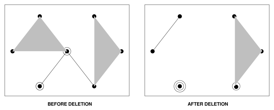
For example, in Figure 1, the patch on the central vertex is selected, and that vertex is removed; this causes a triangular face to collapse to an edge, and two edges incident to the vertex to collapse to patches on the vertices at the other ends. Note that this leaves two patches on the lower left vertex.
If then we say that is obtained from by a (permitted) collapse. Starting from , we can obtain, by a finite sequence of collapses, a stable hypergraph . Denote by the set of vertices removed in passing from to . The elements of are the identifiable vertices. We write for the identifiable hypergraph, given by
We note that , and hence and , do not depend on the particular sequence of collapses chosen. For, if and are two such sequences, and if for all , then we can take minimal and find such that ; then, with an obvious notation, , so must, after all, appear in the terminating sequence , a contradiction. We note also that increases with .
1.5 Purpose of This Paper
The main question we shall address is to determine the asymptotic sizes of and for certain generic random hypergraphs, as the number of vertices becomes large. We note that, since the number of hyperedges is conserved in each collapse, all the identifiable hyperedges eventually turn to debris:
Note that depends only on . In the case where for , the hypergraph min may be considered as a graph on equipped with a number of distinguished vertices. Then is precisely the set of vertices connected in the graph to one of these distinguished vertices.
1.6 Poisson Random Hypergraphs
Let be a probability space. A random hypergraph on is a measurable map
An introduction to random hypergraphs may be found in [11], though we shall pursue rather different questions here. We shall consider a class of random hypergraphs whose distribution is determined by a sequence of non-negative parameters. Say that a random hypergraph on is Poisson if
-
•
The random variables , are independent,
-
•
The distribution of depends only on ,
-
•
Poisson, .
A consequence of these assumptions is that has mean whenever . Note that, when is large, for , only a small fraction of the subsets of size have any hyperedges, and those that do usually have just . Also the ratio of -edges to vertices tends to . Our assumption of Poisson distributions is a convenient exact framework reflecting behaviour which holds asymptotically as under more generic conditions.
1.7 Generating Function
A key role is played by the power series
| (1) |
and by the derived series
Let have radius of convergence . The function may have zeros in but these can accumulate only at 1. Set
| (2) |
and denote by the set of zeros of in . Note that if is a polynomial, or indeed if , then . Also, the generic and simplest case is where is empty.
2 Results
We state our principal result first in the generic case.
2.1 Hypergraph Collapse - Generic Case
Theorem 2.1.
Assume that and . For , let be a set of vertices and let be a Poisson hypergraph on . Then, as , the numbers of identifiable vertices and identifiable hyperedges satisfy the following limits in probability :
Example 2.1.
The random graph with distinguished vertices, described in the introduction corresponds to a Poisson hypergraph , where
and for . Note that and as , where and . Theorem 2.1 extends easily to cases where depends on in such a mild way: one just has to check that Lemma 6.1 remains valid and note that this is the only place that enters the calculations. We have so
Then is the unique such that
and is empty, so in probability as , as stated above.
Example 2.2.
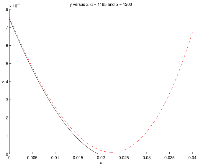
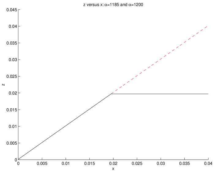
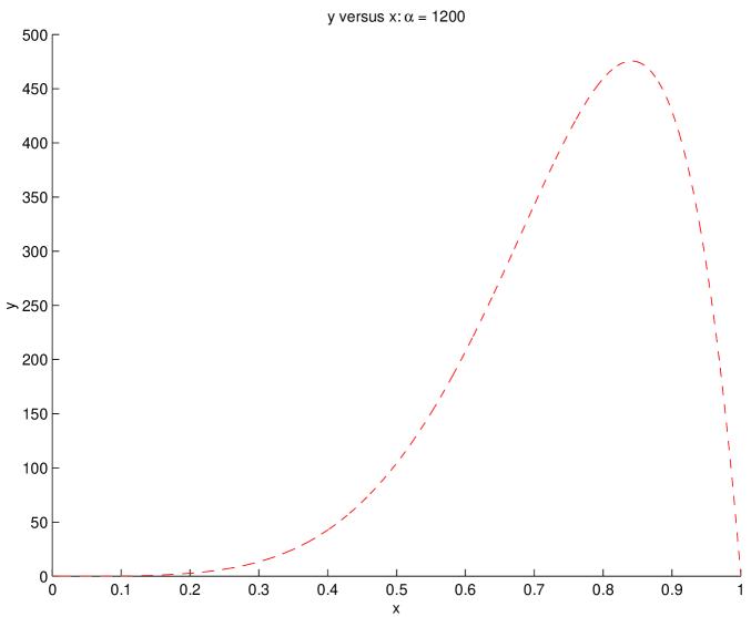
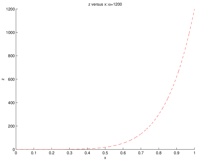
To illustrate critical phenomena, let . Let , , and refer to the re-scaled number of vertices eliminated, the number of patches, and the amount of debris, respectively; here “re-scaled” means after division by the number of vertices. Plots of and versus are shown in Figure 2, for the choices (solid) and (dashed). In the case , hits zero when , and so remains stuck at about 0.02. A very small increase in , from to , causes a dramatic change in the outcome: after narrowly avoiding extinction (Figure 2), the number of patches explodes (Figure 3) as increases towards 1.
Consider what the Figures tell us about the supercritical case : during the first 4% of patch selections, there is rarely any other patch covering the same vertex as the one selected; Figure 3 shows that, during the last 10% of patch selections, an average of other patches cover the same vertex as the one selected. [Read the labels on the -axes carefully: Figure 2 is a close-up of the left-most 4% of the scale of Figure 3.]
|
|
|
|
2.2 Hypergraph Collapse - General Case
In order to describe an extension of Theorem 2.1 to the case where is non-empty, we introduce the random variable
where is a Brownian motion.
Theorem 2.2.
Assume that . Then, for and as in Theorem 2.1, the following limits exist in distribution:
In the case where has only a single point , then is equal to with probability and equal to with probability . We do not know what happens when . Proofs will be given in Section 6.
3 Randomized Collapse
We introduce here a particular random rule for choosing the sequence of moves by which a hypergraph is collapsed, which has the desirable feature that certain key statistics of the evolving hypergraph behave as Markov chains. It is by analysis of the asymptotics of these Markov chains as that we are able to prove our main results.
3.1 Induced Hypergraph
Let be a Poisson hypergraph. For with , let be the hypergraph obtained from by removing all vertices in . Thus, for with ,
where the Poisson parameter is computed as follows: there are ways to choose such that , and the Poisson parameter of is , so
Moreover the random variables , , are independent.
3.2 Rule for Randomized Collapse
Recall that the sequence of vertices chosen to collapse a hypergraph is unimportant, provided we keep going until there are no more patches. However we shall use a specific randomized rule which turns out to admit a description in terms of a finite-dimensional Markov chain. This leads to a randomized process of collapsing hypergraphs . This will prove to be an effective means to compute the numbers of identifiable vertices and identifiable hyperedges for .
The process , together with a sequence of sets such that , is constructed as follows. Let and . Suppose that and have been defined. If there are no patches in , then and . If there are patches in , select one uniformly at random and denote by the corresponding vertex; then set and .
3.3 An embedded Markov chain
Let denote the number of patches and the amount of debris in . Then and for . Also . Let denote the number of other patches at time sharing the same vertex as the st selected patch, and let denote the number of -edges at time containing the st selected vertex . Our analysis will rest on the observation that is a Markov chain, where, conditional on and , we have
and where and with and independent.
To see this, introduce the filtration
Lemma 3.1.
Let
Then
Equivalently, for all so that ,
The claimed Markov structure for follows easily.
Proof.
The identity is obvious for . Suppose it holds for . Let . Take , and . Set and . It will suffice to show, for all hypergraphs having patches and amount of debris , that
where denotes equality up to a constant independent of . But
where the sum is over all hypergraphs which collapse to on removing the vertex . Let denote the number of patches, amount of debris in respectively. Since and are conditionally independent of given and ,
as desired. ∎
4 Exponential Martingales for Jump Processes
We recall here some standard notions for pure jump Markov processes in and their associated martingales. These will be used to study the fluid limit of a sequence of such jump processes in Section 5.
4.1 Laplace Transforms
Let be a pure jump Markov process taking values in a subset of , with Lévy kernel . Consider the Laplace transform
and assume that, for some ,
| (3) |
The distribution of the time and displacement of the first jump of is given by
Introduce random measures and on , given by
where denotes the unit mass at ; is thus the compensator of the random measure , in the sense of [10], p. 422.
4.2 Martingales Associated with Jump Processes
The fact that is a compensator implies that, for any previsible process satisfying
the following process is a martingale
In particular, (3) allows us to take , which gives the martingale
Fix . Then there exists such that
| (4) |
where ′ denotes differentation in . Define for
Then and, for , by the second-order mean value theorem,
so
Let be a previsible process in with for all . Set
| (5) |
Then is locally bounded, and by the Doléans formula ([10], p. 440),
Hence is a non-negative local martingale, so for all . Hence
so is a martingale.
Proposition 4.1.
For all
Proof.
Fix with and consider the stopping time
For , taking for all above, we know that is a martingale. On the set we have . By optional stopping
Hence,
When we can take to obtain
Finally, if , then for one of . ∎
5 Fluid Limit for Stopped Processes
In this section we develop some general criteria for the convergence of a sequence of Markov chains in to the solution of a differential equation, paying particular attention to the case where the chain may stop abruptly on leaving a given open set.
5.1 Fluid Limits
It is possible to give criteria for the convergence of Markov processes in terms of the limiting behaviour of their infinitesimal characteristics. This is a powerful technique which has been intensively studied by probabilists. The book of Ethier and Kurtz [6] is a key reference. Further results are given in Chapter 17 of [10] and in Theorems IX.4.21 and IX.4.26 of [9]. A particular case with many applications is where the limiting process is deterministic and is given by a differential equation, sometimes called a fluid limit. The relevant probabilistic literature, though well developed, may not be readily accessible to non-specialists seeking to apply the results in other fields. One field where fluid limits of Markov processes are beginning to find interesting applications is random combinatorics. Wormald [16] and co-workers have put forward a set of criteria which is specially adapted to this application. The material in this section may be considered as an alternative framework, somewhat more rigid but, we hope, easy to use, developed with the same applications in mind.
Let be a sequence of pure jump Markov processes in . It may be that takes values in some discrete subset of and that its Lévy kernel is given naturally only for . So let us suppose that is measurable, that takes values in , and that the Lévy kernel is given for . Let be an open set in and set . We shall study, under certain hypotheses, the limiting behaviour of as , on compact time intervals, up to the first time the process leaves . In applications, the set will be chosen as the intersection of two open sets and . Our sequence of processes may all stop abruptly on leaving some open set , so that for . If this sort of behaviour does not occur, we simply take . We choose so that the conjectured fluid limit path does not leave in the relevant compact time interval. Subject to this restriction we are free to take as small as we like to facilitate the checking of convergence and regularity conditions, which are required only on .
The scope of our study is motivated by the particular model which occupies the remainder of this paper: so we are willing to impose a relatively strong, large deviations-type, hypothesis on the Lévy kernels , see (6) below, and we are interested to find that strong conclusions may be drawn using rather direct arguments. On the other hand, in certain cases of our model, the fluid limit path grazes the boundary of the set : this calls for a refinement of the usual fluid limit results to determine the limiting distribution of the exit time.
5.2 Assumptions
Consider the Laplace transform
We assume that, for some ,
| (6) |
Set , where ′ denotes the derivative in . We assume that, for some Lipschitz vector field on ,
| (7) |
We write for some Lipschitz vector field on extending . (Such a is given, for example, by where is the Lipschitz constant for .) Fix a point in the closure of and denote by the unique solution to starting from . We assume finally that, for all ,
| (8) |
Whilst these are not the weakest conditions for the fluid limit, they are readily verified in many examples of interest. In particular we will be able to verify them for the Markov chains associated with hypergraph collapse in Section 3.
5.3 Exponential convergence to the fluid limit
Fix and set
Proof.
The following argument is widely known but we have not found a convenient reference. Set and define by
Note that corresponds to the martingale we identified in Proposition 4.1. Fix . Assumption (6) implies that there exists such that, for all ,
Compare this estimate with (4). By applying Proposition 4.1 to the stopped process , we find constants and , depending only on and such that, for all and all ,
| (10) |
Given , set , where is the Lipschitz constant of . Let
Then (8) and (10) together imply that
On the other hand, by (7), there exists such that for all and all . We note that
so, for , on , for ,
which implies, by Gronwall’s lemma, that . ∎
5.4 Limiting Distribution of the Exit Time
The remainder of this section is concerned with the question, left open by Proposition 5.1, of determining the limiting distribution of . Set
It is straightforward to deduce from (9) that, for all ,
| (11) |
In particular, if is empty, then in probability and, for all ,
The reader who wishes only to know the proof of Theorem 2.1 may skip to Section 6 as the remaining results of this section are needed only for the more general case considered in Theorem 2.2.
5.5 Fluctuations
We assume here that
| (12) |
In this case the limiting distribution of may be obtained from that of the fluctuations . We assume that there exists a limit kernel , defined for such that for all and , where
For convergence of the fluctuations we assume
| (13) |
| (14) |
| (15) |
| (16) |
where and . Of course (14) will force .
5.6 Limiting Stochastic Differential Equation
Consider the process given by the linear stochastic differential equation
| (17) |
and starting from , where is a Brownian motion and . The distribution of does not depend on the choice of . For convergence of we assume, in addition,
| (18) |
Theorem 5.1.
Proof.
Let and write the positive elements of as . Define, for ,
where is some cemetery state. We will show by induction, for , that
| (19) |
Given (11), this implies that in distribution, as required.
Note that both and may be considered as time-dependent Markov processes. Hence, by a conditioning argument, it suffices to deal with the case where is non-random. By (18), if , we can assume that is at and . Moreover, for the inductive step, it suffices to consider the case where is non-random, not , and to show that, if in probability, then in distribution. We lose no generality in considering only the case .
We have assumed that in distribution. Note that if and only if and . On the other hand, since , we have if and only if and . Hence in distribution, that is, (19) holds for .
We remark that the same proof applies when the Lévy kernels have a measurable dependence on the time parameter , subject to obvious modifications and to each hypothesis holding uniformly in .
For the remainder of this section, the assumptions of Theorem 5.1 are in force and is non-random.
Lemma 5.2.
For all there exists such that, for all
Proof.
Lemma 5.3.
For all there exists such that, for all , there exists such that, for all and all ,
Proof.
Consider first the case . Given , choose such that, for all , there exists such that, for and
and, with probability exceeding ,
This is possible by (10) and (15). These three inequalities imply
so by Gronwall’s lemma
The case follows by the same sort of argument, using Lemma 5.2 to get the necessary tightness of . ∎
Lemma 5.4.
Suppose either , or and . Then as for some .
Proof.
The case follows from (11). Suppose then that and . Then, since is at , for all , there exists such that, for all with , and all ,
| (20) |
Since , by Lemma 5.3, given there exist and such that, for all and ,
with probability exceeding . Choose so that and whenever . Set , then, for and ,
| (21) |
with probability exceeding . By (20), (21) implies . Hence for all . ∎
For the rest of this section we assume that . (The next result holds with replaced when , by the same argument, but we do not need this.)
Lemma 5.5.
Suppose either , or and . Then in distribution as .
Proof.
By Lemma 5.3, given , we can find such that, for all ,
Hence it suffices to show in distribution for all .
Define in by
Fix and set . Then
so
On the other hand, for as in the proof of Proposition 5.1,
where
By (15),
By (16), given , there exists such that, for all , for ,
Hence and imply
Combining this with Lemma 5.2, we deduce that
Hence it suffices to show, for all and all ,
Indeed, it suffices to show, for all and , that as , where
Set , and
By (14), for all , we have
Note that
so, for all ,
| (22) |
Write , where
Lemma 5.6.
Suppose either , or and . Then, as ,
Proof.
By Lemma 5.5, given , there exists and such that, for all
with probability exceeding . Then by Lemma 5.3, there exists and such that, for all , with probability exceeding , either
| (23) |
or
| (24) |
Since is at , there exists such that
and
Choose such that and whenever . Set . Then, for , since on , (23) implies for all or , and (24) implies or . We know by Lemma 5.4 and (11) that as . Hence, with high probability, as , implies (23) and then , and implies (24) and then . ∎
6 Fluid Limit of Collapsing Hypergraphs
We now apply the general theory from the preceding sections to prove our main results Theorems 2.1 and 2.2.
6.1 Lévy Kernel for Collapse of Random Hypergraphs
In Section 3 we introduced a Markov process of collapsing hypergraphs, starting from Poisson and stopping when , the number of identifiable vertices in . The process of patches and debris in was found itself to be Markov. We now view this process as a function of the initial number of vertices and obtain a fluid limit result when .
It will be convenient to embed our process in continuous time, by removing vertices according to a Poisson process of rate which stops when . Set
and note that takes values in
| (25) |
The Lévy kernel for is naturally defined for . If then . If , then is a probability measure; by Lemma 3.1, it is the law of the random variable , where
with and independent.
Recall that denotes the radius of convergence of the power series , given by (1). We assume, until further notice, that and fix and .
Lemma 6.1.
There is a constant such that
for all and .
Proof.
Recall that
Set where . Then, for ,
where
and
Note that, for and ,
so, making use of the inequality for , we obtain
Hence
and . ∎
6.2 Fluid Limit
The main result of this section is to obtain the limiting behaviour of as , which we deduce from Proposition 5.1 and Theorem 5.1. We present first the calculations by which the limit was discovered.
Note that, as , for , we have and in distribution, where
Set . Note also that in distribution, where , , with and independent. Thus, subject to certain technical conditions, to be checked later, at least up to the first time that or , the limit path is given by , starting from , where
Fix and set
| (26) |
then is Lipschitz on and, for sufficiently large, the maximal solution on to in starting from is given by , where
and
6.3 Limiting Fluctuations
Set . A convenient choice of such that is , where
Note that is a Lipschitz and is on . The limiting fluctuations are given by
starting from , where is a Brownian motion in independent of . Note that
In cases where is non-empty, the limiting behaviour of depends on the signs of the component of the fluctuations normal to the boundary, that is, on .
Note that satisfies
This is the part of the fluctuations which reflects our Poissonization of the time-scale. Since for all , it does not affect . So consider . Then
Note that and , so for all . Also and . Also and . The sign of is the same as that of . We have
so we can write , where is a Brownian motion and
We have shown that has the same distribution as In particular for all .
Recall that is defined by
Set
and put , .
Theorem 6.1.
For all we have
Moreover, in distribution as .
Proof.
We defined , the state-space of , in (25), and in (26). Set . For we have
so
where, for , we write and . So, by Lemma 6.1,
as , for all , where
Set
then, by Lemma 7.1,
Recall that
and . By standard exponential estimates, for all
We have now checked the validity of (7), (8), (12), (13), (14), (15), (16), (18) in this context, so Proposition 5.1 and Theorem 5.1 apply to give the desired conclusions. ∎
6.4 Proof of Theorem 2.2
Proof.
Recall that
Let . If , then so, by choosing in Theorem 5.1, we obtain
| (27) |
for all sufficiently small
It remains to deal with the case . Note that and . Now so in probability as . It therefore suffices to show, for all and ,
When combined with (27) this completes the proof as we have exhausted the possible values of .
We consider first the case . We can find such that . Note that implies
By Theorem 6.1
so we are done.
Consider next the case . Fix and set if and otherwise. Then, with obvious notation, we can choose so that , and . Hence
We can couple and so that . Then and , so this is enough.
There remains the case . In this case is finite. We have assumed that . So we can find and such that, with obvious notation,
where , is defined by
Consider the collapsing hypergraph which evolves as up to , at which time all hyperedges having at least two vertices and originally having more than vertices are removed, so that . After evolves by selection of patches as before. Denote by the set of identifiable vertices in and by the corresponding identifiable hypergraph. Then
A modification of Theorem 5.1 shows that
with and with
All that changes in the proof is that, for the Lévy kernel is modified by replacing by given by
The argument of Lemma 6.1 shows that for all there is a constant such that
for all and . Everything else is the same.
Now implies
so
as required. ∎
Acknowledgments. The authors thank the Mathematisches Forschungsinstitut Oberwolfach for the invitation to the meeting in 2000 at which this collaboration began, and Brad Lackey for his interest in this project. David Levin helped us to articulate some of the concepts presented herein.
References
- [1] Achlioptas, Dimitris, Lower bounds for random 3-SAT via differential equations. Phase transitions in combinatorial problems (Trieste, 1999). Theoret. Comput. Sci. 265 (2001), no. 1-2, 159–185. MR1848217
- [2] Achlioptas, Dimitris; Kirousis, Lefteris M.; Kranakis, Evangelos; Krizanc, Danny Rigorous results for random -SAT Phase transitions in combinatorial problems (Trieste, 1999). Theoret. Comput. Sci. 265 (2001), no. 1-2, 109–129. MR1848214
- [3] Bollobás, B., Random graphs. Academic Press, London, 1985.
- [4] Coppersmith, Don; Gamarnik, David; Hajiaghayi, Mohammad; Sorkin, Gregory B. Random MAX SAT, random MAX CUT, and their phase transitions. Proceedings of the Fourteenth Annual ACM-SIAM Symposium on Discrete Algorithms (Baltimore, MD, 2003), 364–373, ACM, New York, 2003. MR1974940
- [5] Darling, R.W.R.; Levin, D.A.; Norris, J. R., Continuous and discontinuous phase transitions in hypergraph processes. Preprint. http://xxx.lanl.gov/abs/math.PR/0312451
- [6] Ethier, S. N.; Kurtz, T. K., Markov processes: characterization and convergence. Wiley Series in Probability and Mathematical Statistics. Wiley, New York, 1986.
- [7] Duchet, Pierre, Hypergraphs. Handbook of Combinatorics, edited by R. Graham, M Grötschel, L. Lovász, Elsevier Science B.V., 1995
- [8] Erdős, P.; Rényi, A., On the evolution of random graphs. Magyar Tud. Akad. Mat. Kutató Int. Közl., 5, (1960), 17–61.
- [9] Jacod, J.; Shiryaev, A. N., Limit Theorems for Stochastic Processes. Springer, Berlin, 1987
- [10] Kallenberg, O., Foundations of Modern Probability. Springer, New York, 1997.
- [11] Karoński, M.; Łuczak, T., Random hypergraphs. Combinatorics, Paul Erdös is eighty, Vol. 2 (Keszthely, 1993), 283–293, Bolyai Soc. Math. Stud., 2, János Bolyai Math. Soc., Budapest, 1996. [97m:05232]
- [12] Kordecki, Wojciech, On the connectedness of random hypergraphs. Comment. Math. Prace Mat. 25 (1985), no. 2, 265–283. [87k:05140]
- [13] Norris, J.R., Cluster coagulation. Commun. Math. Phys. 209 (2000), 407–435.
- [14] Schmidt-Pruzan, Jeanette; Shamir, Eli, Component structure in the evolution of random hypergraphs. Combinatorica 5 (1985), no. 1, 81–94. [86j:05106]
- [15] Wilson, David B. On the critical exponents of random -SAT. Random Structures and Algorithms 21 (2002), no. 2, 182–195. MR1917357
- [16] Wormald, Nicholas C., Differential equations for random processes and random graphs. Annals of Applied Probability 5 (1995), no. 4, 1217–1235. [97c:05139]