The Goda-Teragaito conjecture: an overview

Abstract.

We give an overview of the proof ([Sc]) that the only knots that are both tunnel number one and genus one are those that are already known: $2$-bridge knots obtained by plumbing together two unknotted annuli and the satellite examples classified by Eudave-Muñoz and by Morimoto-Sakuma.

1. Preliminaries

Definition 1.1.

A graph $\mbox{$\Gamma$}\subset S^{3}$ is a Heegaard spine if it has a regular neighborhood $H\subset S^{3}$ so that $S^{3}-interior(H)$ is a handlebody.

Note that $\Gamma$ is a Heegaard spine if and only if the decomposition $S^{3}=H\cup_{\mbox{$\partial$}H}(S^{3}-\mbox{${\rm interior}$}(H))$ is a Heegaard splitting of $S^{3}$.

Definition 1.2.

A theta-graph $\theta\subset S^{3}$ is an embedded graph consisting of two vertices and three edges, each edge incident to both vertices. A knot $K\subset S^{3}$ has tunnel number one if there is a theta-graph $\theta\subset S^{3}$ so that

• $\theta$ is a Heegaard spine

• for some edge $\tau\subset\theta$, $K=(\theta-\mbox{${\rm interior}$}(\tau))$

The edge $\tau$ is called the unknotting tunnel for $K$.

Definition 1.3.

A knot $K$ has genus one if there is a PL once-punctured torus $F\subset S^{3}$ so that $K=\mbox{$\partial$}F$. That is, $K$ has a Seifert surface $F$ of genus one.

Both sorts of knots, those of tunnel number one and those of genus one, have pleasant and useful properties. Although each type can be quite complicated (as measured, for example, by crossing number), each is in some sense the first and easiest collection of knots under one natural index of complexity (the tunnel number or the genus). It’s therefore of interest to determine which knots are simple in both senses. That is, which knots have both tunnel number one and genus one.

The answer, as earlier conjectured by Goda and Teragaito [GT] is this:

Theorem 1.4.

[Sc] Suppose $K\subset S^{3}$ has tunnel number one and genus one. Then either

1. $K$ is a satellite knot or

2. $K$ is a $2$-bridge knot.

This theorem is useful because of the historical background: $2$-bridge knots all have tunnel number one and those of genus one are easily described (cf [BZ, Proposition 12.25]) and, indeed, they are easily pictured: see Figure 1.

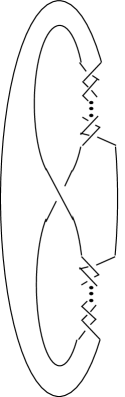
Figure 1.

On the other hand, Morimoto and Sakuma [MS] and independently Eudave-Muñoz [EM] classified all satellite knots which have tunnel number one. These knots have a concrete description and can be naturally indexed by a $4$-tuple of integers. In [GT], Goda and Teragaito determined which of these satellite knots have genus one and made the conjecture that these knots complete the list of knots that have both genus one and tunnel number one. In other words, they conjectured that Theorem 1.4 is true.

The proof that the conjecture is true, as given in [Sc], is long and intricate but much of the energy and length is required by arguments that are in some sense technical. The intention here is to give an overview of the proof that focuses on general strategy. The hope is that the reader will understand how the proof follows a rather natural course, not one that is as contrived as it might first appear.

2. The mathematical background

Matsuda had verified the Goda-Teragaito conjecture (Theorem 1.4) for an important class of knots, and we will need his result. A useful way to state it for our purposes is this:

Theorem 2.1.

[Ma] Suppose that $\tau$ is an unknotting tunnel for the genus one knot $K$ and one of the cycles in the theta-graph $K\cup\tau$ is the unknot. Then $K$ is either a satellite knot or a $2$-bridge knot.

This special case is more general than it might seem. Suppose, for example, that $H$ is a regular neighborhood of a theta-curve Heegaard spine $\theta$, so $H$ is a genus two handlebody. Associated to each edge $e$ in $\theta$ is a meridian disk $\mu_{e}\subset H$ that intersects $e$ in a single point. We have this corollary of Matsuda’s theorem:

Corollary 2.2.

Suppose that $K$ is a genus one knot lying on $\mbox{$\partial$}H$ that intersects $\mu_{e}$ in a single point. Suppose further that $\theta-\int(e)$ is the unknot. Then $K$ is either a satellite knot or a $2$-bridge knot.

Proof.

Apply the “vacuum cleaner trick” to the $1$-handle in $H$ corresponding to the edge $e$. That is, think of $K$ as the union of two arcs: one arc $\alpha$ runs exactly once over the $1$-handle, and the other arc $\beta$ lies on the boundary of the unknotted solid torus $W=H-(1$-$handle)$ and $\beta$ connects the ends of $\alpha$ in $\mbox{$\partial$}W$. Slide the ends of the $1$-handle along the arc $\beta$, vacuuming it up onto the $1$-handle until $K$ has been made disjoint from a meridian disk $\mu$ of $W$. At this point, $H$ can be viewed as the regular neighborhood of another $\theta$-graph, namely $K\cup\tau$, where $\tau$ is an edge intersecting $\mu$ in a single point (i. e. $\mu=\mu_{\tau}$). Since $W$ is an unknotted torus, the corresponding cycle in $\theta$ is unknotted and Theorem 2.1 applies. ∎

An unexpected application of Corollary 2.2 arises from work of Eudave-Muñoz and Uchida. Suppose that $H$ is a regular neighborhood of a theta curve $\theta$ that is a Heegaard spine. Let $X=S^{3}-\mbox{${\rm interior}$}(H)$, a genus two handlebody. Suppose that $F$ is a properly imbedded incompressible genus one surface in $X$ with $\mbox{$\partial$}F=K=F\cap\mbox{$\partial$}H$.

Proposition 2.3.

Let $A\subset X$ be an incompressible annulus obtained from $F$ by $\partial$-compressing $F$ to $\mbox{$\partial$}H=\mbox{$\partial$}X$. Suppose there is an edge $e$ of $\theta$ so that $|\mu_{e}\cap\mbox{$\partial$}A|=1=|\mu_{e}\cap K|$. Then $K$ is either a satellite knot or a $2$-bridge knot.

Proof.

$\mbox{$\partial$}A$ has two components which we denote $\mbox{$\partial$}_{\pm}A$ and we take $\mbox{$\partial$}_{-}A$ to be the component that intersects $\mu_{e}$. Take two parallel copies of $\mu_{e}$ and band them together along the part of $\mbox{$\partial$}_{-}A$ that does not lie between them. The result is a disk $E\subset H$ that is disjoint from $\mbox{$\partial$}A$ and separates $H$, leaving one of $\mbox{$\partial$}_{\pm}A$ in the boundary of each of the solid tori components of $H-E$. Label these solid tori correspondingly $L_{\pm}$ and denote by $L$ the link whose core circles are $L_{-}\cup L_{+}$. Note that $\mbox{$\partial$}_{-}A$ is a longitude of $L_{-}$ and $\mbox{$\partial$}_{+}A$ is a $(p,q)$ cable of $L_{+}$, for some $(p,q)$.

The link $L$ visibly has an incompressible annulus (namely $A$) in its complement. Moreover, $L$ has tunnel number one: attaching to $L$ an edge dual to $E$ gives a graph $\Gamma$ whose regular neighborhood is $H$, so $\Gamma$ is a Heegaard spine. Tunnel number one links with essential annuli in their complement have been classified by Eudave-Muñoz and Uchida (cf. [EU]). In particular, $L_{+}$ is the unknot. But $L_{+}$ can also be viewed as the cycle in $\theta$ obtained by removing $e$ (equivalently, the core of the torus obtained by removing $\mu_{e}$). Since $|\mu_{e}\cap K|=1$, the result follows from Corollary 2.2. ∎

A special case of this proposition is independently useful:

Corollary 2.4.

Suppose $\tau$ is an unknotting tunnel for $K$ and $\tau$ lies on a genus one Seifert surface $F$ for $K$. Then $K$ is either a satellite knot or a $2$-bridge knot.

Proof.

$\tau$ can’t be parallel to a subarc of $K$, else $K$ would itself be unknotted. So $\tau$ is an essential arc in $F$, and so $F-\eta(\tau)$ is an annulus. Let $H$ be a regular neighborhood of the theta-graph $K\cup\tau$ and $\mu$ be a meridian disk for $K$, considered also as a meridian dual to an edge of the graph $K\cup\tau$. Then $F-\mbox{${\rm interior}$}(H)$ is an incompressible annulus $A$ that satisfies the hypotheses of Proposition 2.3. ∎

The last proposition and its corollary begin to suggest a strategy for trying to prove the conjecture: Let $\theta=K\cup\tau$. Try to arrange that $\tau$ is disjoint from a genus one Seifert surface $F$ for $K$, so that we can think of $F$ as lying in the closed complement $X$ of $H=\eta(\theta)$ in $S^{3}$. This makes $F\cap\mbox{$\partial$}H$ a useful copy of $K$ lying on $\mbox{$\partial$}H$. Try to show that some boundary-compressing disk for $F$ in $X$ crosses a meridian of $\tau$ exactly once or, alternatively, is disjoint from a meridian corresponding to one of the two edges $K-\tau\subset\theta$. If the former happens then, with some work, $\tau$ can be isotoped onto $F$ and Corollary 2.4 applies. If the latter happens then we can invoke Proposition 2.3.

Such a strategy requires an understanding of potential boundary-compressing disks for $F$ in $X$, once $\tau$ is made disjoint from $F$. A natural source for such disks are the outermost disks cut off by $F$ from meridians of the handlebody $X$. That is, if $E$ is a meridian disk of $X$, then an outermost arc of $E\cap F$ in $E$ cuts off a disk $E_{0}$. Moreover, $E_{0}$ lies on one side of $F$, so the arc $\omega=E_{0}\cap\mbox{$\partial$}H$ has both ends incident to the same side of $K$. Consider the meridians $\mu_{\pm}$ of $H$ corresponding to the two edges of $\theta=K\cup\tau$ coming from $K$ and the meridian $\mu^{t}$ coming from the edge $\tau$. If $\omega$ is disjoint from either of the meridians $\mu_{\pm}$ then we are done by Proposition 2.3. If $\omega$ intersects both these meridians, then some subarc $\omega_{0}$ of $\omega$ cut off by $\mu_{\pm}$ is an arc in the $4$-punctured sphere $\mbox{$\partial$}H-\mu_{\pm}$ running from a copy of $\mu_{-}$ to $\mu_{+}$. Arcs in a $4$-punctured sphere are easy to understand – each roughly corresponds to a rational number given by its slope, viewing the $4$-punctured sphere as a pillowcase with holes in the corners. See Figure 2 Since $\omega_{0}$ is disjoint from the vertical (i. e. slope $\infty$) arcs $K\cap\mbox{$\Sigma$}$, it determines a non-zero integral slope which (by appropriate choice of slope $0$) we may take to be $1$. In other words, we are done unless the meridian disks of $X$ intersect the $4$-punctured sphere $\mbox{$\partial$}H-\mu_{\pm}$ in arcs of one particular slope.

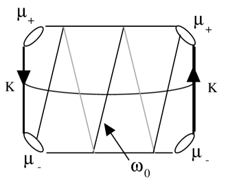
Figure 2.

Of course the genus two handlebody $X$ has many meridians, so it seems that it would be difficult to say much about the slopes of arcs determined by these meridians. But it is a remarkable fact (see [ST1]) that, if we restrict to simple closed curves in $\mbox{$\partial$}H$ that bound meridians in both $H$ and $X$, the slope is determined (up to only a small ambiguity) by $K$ and $\tau$, as long as $K$ is not $2$-bridge. We are done anyway if $K$ is $2$-bridge, so the upshot is that right from the beginning there is only one troublesome case to deal with – when the slope given by a meridian of $X$, a meridian whose boundary also bounds a meridian of $E$, is simply $1$. The argument here is more rigorously presented in [ST1] (where what we here call the “slope” is there the invariant $\mbox{$\rho$}\in\mathbb{Q}/2\mathbb{Z}$).

This completes the proof of the Goda-Teragaito conjecture for all but the case $\mbox{$\rho$}=1$. But this final case seems to require a substantial broadening of our strategy which we now describe. Roughly, we start with $H=\eta(K\cup\tau)$ but find simpler and simpler spines for $H$, allowing $K$ to appear more complex on $\mbox{$\partial$}H$ with respect to these simpler spines. The hope is to do this in such a controlled manner that much of the argument above can still be applied and, moreover, the process does not stop until one of the cycles in the spine is the unknot.

3. The psychological background - thin position and its successes

The notion of thin position for knots goes back to early work of Gabai ([G]). In outline, the idea is this: Think of $S^{3}$ as swept out by an interval’s worth of $2$-spheres. More concretely, choose a height function $h:S^{3}\mbox{$\rightarrow$}[-1,1]$ with exactly two critical points: a maximum and a minimum at heights $\pm 1$. It is possible to associate a natural number, called the width, to any generic positioning of a knot $K$ in $S^{3}$. This can be done so that the width is unchanged by isotopies of $K$ that do not create or destroy critical points or change the ordering of the heights of the critical points. In fact, width stays unchanged if the height of two adjacent maxima or two adjacent minima are switched. It will go down if a maximum is pushed below a minimum or a maximum and a minimum are cancelled. When the width is minimized, the knot is said to be in thin position.

To illustrate the usefulness of thin position, consider a knot $K\subset S^{3}$ in thin position and suppose $F$ is an incompressible Seifert surface for $K$. Suppose some level $2$-sphere $P$ (ie $P=h^{-1}(t),t\in(-1,1)$) is transverse to $F$ and among the components of $F-P$ are a pair of disks, say cut off by arc components of $P\cap F$, one disk lying above $P$ and one below $P$. Then those disks would describe a way to simultaneously push a maximum of $K$ below $P$ and a minimum of $K$ above $P$, reducing the width. We conclude that no such pair of disks occurs.

On the other hand, as we imagine level spheres $P_{t}=h^{-1}(t)$ sweeping across $F$ from top to bottom, at first there must be a disk cut off from $F$ that lies above $P_{t}$ and just before the end of the sweep there must be a disk from $F$ that lies below $P_{t}$. Since there can’t simultaneously be both types of disks, as we have just seen, there must be some height at which there are no disks of either type, so in fact for $P$ at this height, all components of $P\cap F$ are essential in $F$.

If $F$ is of genus one, then essential $1$-manifolds in $F$ are easy to describe. For example, if all components of the $1$-manifold are arcs then these arcs lie in at most three different parallelism classes.

In [GST] we presented a similar notion of thin position that works well for trivalent graphs in $S^{3}$. That is, just as for knots, it is possible to define the width of a generic positioning of a trivalent graph $\Gamma$ in $S^{3}$ in such a way that the width is unchanged by isotopies of $K$ that do not create or destroy critical points or change the ordering of the heights of the critical points, where here “critical point” is enlarged to include vertices of the graph. Moreover, and this is the delicate point, the width stays unchanged if the height of two adjacent maxima or two adjacent minima are switched. Here the delicacy arises because the maxima (and minima) can be of two different types: one type is the standard maximum of an arc, but the second type is that of a $\lambda$-vertex, i. e. a vertex incident to two ends of edges lying below it and one above. The last crucial property of the width is that, just as in the case of knots, the width of $\Gamma$ will go down if a maximum is pushed below a minimum or a maximum and a minimum are cancelled, or a $\lambda$-vertex and adjacent standard minimum become a $Y$-vertex (or, symmetrically, a $Y$-vertex and adjacent standard maximum become a $\lambda$-vertex). To summarize briefly: If $\Gamma$ is in thin position then, without affecting width, minima can be pushed past other minima and maxima past other maxima but no maximum can be pushed below any minimum.

It turns out that any theta-curve Heegaard spine in $S^{3}$ has a useful property when it is put in thin position.

Definition 3.1.

A trivalent graph $\mbox{$\Gamma$}\subset S^{3}$ is in bridge position with respect to a height function $h:S^{3}\mbox{$\rightarrow$}[-1,+1]$ if there is a level sphere $P\subset S^{3}$ so that all maxima of $\Gamma$ lie above $P$ and all minima lie below. Such a sphere $P$ is called a dividing sphere.

Theorem 3.2.

[ST2] Suppose $\theta\subset S^{3}$ is a theta-curve Heegaard spine that is in thin position in $S^{3}$. Then $\theta$ is in bridge position and some edge of $\Gamma$ is disjoint from a dividing sphere.

With this in mind, we try to extend the application of thin position given above to the following: Suppose $\theta$ is a theta-curve Heegaard spine with regular neighborhood $H$ and the Seifert surface $F$ is properly embedded in $X=S^{3}-\mbox{${\rm interior}$}(H)$. Suppose $\theta$ is in thin position and $K$ doesn’t “back-track” along any edge in $\theta$. That is, $K$ doesn’t intersect twice in a row the meridian corresponding to any one edge of $\theta$. Then, just as in the case for thin position of knots, there is a level sphere $P$ that intersects $F$ only in essential curves. It turns out that the following example of this situation (the motivation will come a bit later) is crucial:

Definition 3.3.

Suppose $\theta$ is a theta-curve in $S^{3}$ with edges $e^{+},e^{-},e^{\bot}$. In $H=\eta(\theta)$, denote the corresponding meridians by $\mbox{$\mu^{+}$},\mbox{$\mu^{-}$},\mbox{$\mu^{\bot}$}$. Suppose $K\subset\mbox{$\partial$}H$ is a primitive curve in $\mbox{$\partial$}H$ (i. e. it intersects some essential disk in $H$ in a single point) and $K$ intersects each of the meridians $\mbox{$\mu^{+}$},\mbox{$\mu^{-}$},\mbox{$\mu^{\bot}$}$ always with the same orientation and so that some minimal genus Seifert surface $F$ for $K$ intersects $H$ only in $K=\mbox{$\partial$}F$. Arrange the labelling and orientations of the edges and meridians so that, geometrically as well as algebraically,

• $K\cap\mbox{$\mu^{-}$}=q\geq 1$

• $K\cap\mbox{$\mu^{+}$}=p\geq q$

• $K\cap\mbox{$\mu^{\bot}$}=p+q$.

Then we say that $K$ (or $(K,F)$) is presented on $\theta$ as a $(p,q)$ quasi-cable.

Our remarks above then show that if $\theta$ is in thin position and $(K,F)$ is presented on $\theta$ as a $(p,q)$ quasi-cable then some level sphere $P$ intersects $F$ in a $1$-manifold that is essential in $F$. If $F$ is of genus one then the components of $F\cap P$ fall into at most three parallelism classes in $F$. It is not obvious, but is not difficult to show, that this greatly constrains the kind of $(p,q)$ quasi-cabling that can give rise to genus one surfaces. Most importantly (see [Sc, Lemma 2.3]) the constraint forces $q=1$. In the context of the strategy outlined above (cf. Corollary 2.2 and Proposition 2.3) establishing that a meridian dual to an edge intersects $K$ exactly once is a promising development indeed. Indeed, this connection alone suggests that thinking about $K$ as a $(p,q)$ quasi-cable could be quite useful.

Next we show why it is not only useful but also perhaps natural to think about $K$ as a $(p,q)$ quasi-cable. For this we go back to the argument of Section 2 and consider how we might try to apply thin position to the only case ($\mbox{$\rho$}=1$) in which the argument of Section 2 fails. Recall that $\mbox{$\rho$}=1$ means that for $E$ any meridian of $X$, there is an arc $\omega_{0}\subset\mbox{$\partial$}E$ running between the pair of meridians $\mu_{\pm}$ such that $\omega_{0}$ is disjoint from $K$. Now suppose the theta-graph $\theta=K\cup\tau$ is put in thin position and, moreover, among all possible ways of sliding $\tau$ on $K$, we’ve picked the one that makes $\theta$ thinnest. We hope to use the thin position argument formerly applied to the Seifert surface $F$ and see what happens if we apply it instead to the meridian disk $E$.

A first observation is that, following [GST], we can assume that $K\cup\tau$ is in bridge position and that a dividing sphere is disjoint from the tunnel $\tau$. Indeed it is shown in [GST] that, with $K$ in bridge position, the tunnel $\tau$ may be made level with its ends at maxima (or minima). If, when $\tau$ made level, the ends of the tunnel are at the same maximum, then the tunnel is unknotted and we can appeal to Theorem 2.1 to complete the argument. If instead the tunnel $\tau$ has its ends at different maxima then the small perturbation that makes $K\cup\tau$ generic will leave it in bridge position, with $\tau$ monotonic and above the dividing sphere.

Figure 3.

Consider now how level spheres would intersect a meridian disk $E$ of $X$ as they sweep across $\theta$. We saw that as they sweep across $F$ there is at least one level at which the intersection with $F$ is an essential collection of curves in $F$. Something must go wrong with this argument when we replace $F$ with $E$, for it is impossible to have essential arcs in a disk like $E$. It’s easy to see what can go wrong: it may be that there is a level sphere $P$ that simultaneously cuts off both lower and upper disks from $E$, but these disks are incident to $H$ in such a complicated way that they can’t be used to make $\theta$ thinner. Such a complicated arc can only arise when some component of $\mbox{$\partial$}H-P$ is itself complicated, eg the $4$-punctured sphere component $\Sigma$ of $\mbox{$\partial$}H-P$ that appears when $P$ is a dividing sphere. (See Figure 3.) In particular, we founder when two conditions occur: some subarc $\omega_{0}$ of $\mbox{$\partial$}E$ is relatively simple in $\Sigma$ (so that $\mbox{$\rho$}=1$), while another subarc (namely the arc on which an upper disk is incident to $\Sigma$) is relatively complex. Since these subarcs are disjoint (for $\mbox{$\partial$}E$ is embedded) the possibilities are few. In fact, and this is not obvious, the most difficult case to handle is one in which the upper disk is so positioned that it defines a way in which $\theta$ can only be made thinner by a Whitney move on the edge $\tau$. This Whitney move has the effect of placing $K$ on $\mbox{$\partial$}H$ as a $(1,1)$-quasi-cable; see [Sc, Lemma 5.5] and Figure 4. So we naturally move to thinking about $K$ as a quasi-cable on some different spine of $H$.

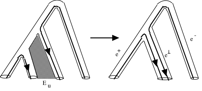
Figure 4.

This Whitney move begins a kind of inductive process. We try to repeat the argument in the more general setting in which $(K,F)$ is presented as a quasi-cable on the neighborhood $H$ of a theta-curve Heegaard spine. The knot $K$ is kept thinly presented thorughout the process and the strategy is to choose the thinnest possible theta-curve for such a presentation. If such a thinnest theta-curve $\theta$ contains an unknotted cycle, then (essentially) Corollary 2.2 can be applied to finish the proof. If it doesn’t, then we try to use a meridian $E$ of $X$ to thin $\theta$ further and observe that it will do so unless, as previously, $\theta$ is in bridge position, some edge of $\theta$ is disjoint from a dividing sphere, and some such dividing sphere $P$ cuts off both an upper disk $E_{u}$ and a lower disk $E_{l}$ from $E$.

We then consider again how $\mbox{$\partial$}E$ intersects the $4$-punctured sphere component $\mbox{$\Sigma$}\subset\mbox{$\partial$}H$ of $\mbox{$\partial$}H-P$. If a $\partial$-compressing disk $E_{0}$ for $F$ in $X$ cut off from $E$ by $F$ is incident to $\mbox{$\partial$}H$ in an arc $\omega$ so short that $\omega$ lies entirely in $\Sigma$, then the annulus $A$ resulting from the $\partial$-compression naturally satisfies the hypothesis of Proposition 2.3, so we would be done. The remaining possibility is that the arc $\omega\subset\mbox{$\partial$}E$ to which $F$ $\partial$-compresses is long. That is, the subarc $\omega$ of $\mbox{$\partial$}E$ is disjoint from $K$, has both its ends on the same side of $K$ but passes through $\Sigma$ perhaps many times. (We can assume that the ends of $\omega$ both lie in $\Sigma$.) The hope would be that this relatively clear picture of $\omega$ would be enough to show that the upper and lower disks $E_{u}$ and $E_{l}$ could either be used to thin $\theta$ further (a contradiction) or at least would describe how to perform a Whitney move that would thinly present $K$ as a (possibly more complicated) quasi-cable on an even thinner theta-graph. If this last step works (as it did in the simple case $\theta=K\cup\tau)$ then when we reach the thinnest possible theta-graph that presents $(K,F)$ as a quasi-cable we will be done. Either a cycle in the theta-graph is unknotted and we are done by a version of Corollary 2.2 or the arc $\omega$ lies entirely in $\Sigma$ and we are done by Proposition 2.3.

4. Refinements and combinatorial arguments

The last step in the program outlined in Section 3 is to exploit upper and lower disks $E_{u}$ and $E_{l}$ cut off from a meridian disk $E$ of $X$ by a level sphere $P$. The hope is that $E_{u}$ and $E_{l}$ can be used either to thin $\theta$, or at least to perform a useful Whitney move on $\theta$. Just about all we know about the disks $E_{u}$ and $E_{l}$ is that they are disjoint from a long arc we’ve called $\omega$ that is itself disjoint from $K$ and has ends incident to $K$ from the same side. We can also assume (from thin position) that $P$ lies below an entire edge of $\theta$, so the corresponding component $\Sigma$ of $\mbox{$\partial$}H-P$ is a $4$-punctured sphere.

Things seems rather hopeless, especially if the edge that is disjoint from $P$ is $e^{\bot}$: The definition of quasi-cable means that no subarc of $K$ goes directly from $e^{+}$ to $e^{-}$. In particular, an arc in $\mbox{$\partial$}H$ can “backtrack” at an end of $e^{\bot}$ without necessarily intersecting $K$. That is, there is an essential arc in $\mbox{$\partial$}H-K$ with both ends on $\mu^{\bot}$ and with interior disjoint from both of the other meridians $\mu^{\pm}$. See Figure 5. This means that, for all we know, the long arc $\omega$ could traverse $\Sigma$ in a complicated way, passing many times across the meridian $\mu^{\bot}$ and still $\omega$ could be disjoint from $K$. If $\omega$ can be this complicated, there is nothing to prevent $\mbox{$\partial$}E_{u}$ from traversing $\Sigma$ in an equally complicated way and so it would be useless either for thinning or for describing a simple Whitney move.

Figure 5.

Here’s an approach to fixing this problem, at least: To ensure that no arc of $\mbox{$\partial$}E$ backtracks at an end of $e^{\bot}$, somehow guarantee that $\mbox{$\partial$}E$ does backtrack at both ends of another edge, one of $e^{\pm}$, for then no backtracking arc at an end of $e^{\bot}$ could be disjoint from $\mbox{$\partial$}E$. Requiring that $\mbox{$\partial$}E$ backtracks on one of the other edges $e^{\pm}$ is more reasonable than it might appear: Recall that $E$ could have been chosen so that its boundary also bounds a disk $D\subset H$. If we consider how $D$ intersects the meridians $\mbox{$\mu^{\pm}$},\mbox{$\mu^{\bot}$}$ of $H$, an outermost arc of intersection on $D$ will precisely cut off a backtracking arc from $\mbox{$\partial$}D=\mbox{$\partial$}E$. So we know that there is a back-tracking arc (called a wave) on exactly one edge. So the refinement needed to avoid backtracking at an end of $e^{\bot}$ is to insist that we will only consider theta-graphs which present $(K,F)$ as a quasi-cable and which also satisfies the wave condition; that is, we require that there is a wave of $\mbox{$\partial$}E$ based at one of the meridians $e^{\pm}$. Of course, this restriction means that the inductive step (i. e. the Whitney move) must be shown to preserve the wave condition at the next stage, including the first stage in which $K\cup\tau$ becomes a theta graph presenting $(K,F)$ as a $(1,1)$ cable. Checking this is a bit technical and we only note here that it is shown in [Sc] that it can be done.

Introducing the wave condition gives unexpectedly useful information about the long arc $\omega$. If, for example, a wave is based at the meridian $\mu^{+}$ of $e^{+}$ then $\omega$ can’t pass directly from an end of $e^{-}$ to an end of $e^{\bot}$ since a wave is in the way, nor can it backtrack on any edge, for even in backtracking at an end of $e^{+}$ it would cross $K$. It follows, for example, that $\omega$ always crosses each meridian $\mbox{$\mu^{\pm}$},\mbox{$\mu^{\bot}$}$ in the same direction. Even more (somewhat technical) information is available about $\omega$ and hence about the boundary of the annulus $A$ that is obtained from $F$ by $\partial$-compressing to $\omega$, but what we’ve described is enough to give an outline of the rest of the argument.

The first observation is that, if $\mbox{$\alpha$}_{u}=E_{u}\cap\mbox{$\partial$}H$ were actually parallel to a segment of $\omega\cap\mbox{$\Sigma$}$ we would be nearly finished: Since $\omega$ doesn’t backtrack along any edge, there are only a few paths it can take through $\Sigma$; if $\mbox{$\alpha$}_{u}$ also took one of these paths, then it’s relatively easy to show that $E_{u}$ and $E_{l}$ describe a way either to thin $\theta$ or to perform an appropriate Whitney move (depending on the path). It turns out that, when the edge of $\theta$ that is disjoint from $P$ is the edge that contains the wave, just knowing that the wave is disjoint from $\omega$ suffices to show there is an appropriate Whitney move. So, for a good representative of the hard cases that remain, we assume that it is the edge $e^{\bot}$ that is disjoint from the dividing sphere $P$.

Now a brief digression. We’ve noted above that if $\mbox{$\alpha$}_{u}$ were parallel to a segment of $\omega\cap\mbox{$\Sigma$}$ we would be finished. This suggests (and one can prove) that there is a dividing sphere $P$ that intersects the annulus $A$ only in essential spanning arcs. Roughly, the argument is the standard thin position argument: if, as $P_{t}$ sweeps across $\theta$, there were always some inessential arc of intersection then at some level there would be a dividing sphere that cut off both an upper and a lower disk from $A$. But $\mbox{$\partial$}A$ does follow (roughly) $\omega$, since $\mbox{$\partial$}A$ is obtained by banding $K$ to itself along $\omega$. Now these two disks could be used, either to thin $\theta$ or to perform an appropriate Whitney move, changing $\theta$ to a thinner graph which still presents $(K,F)$ as a quasi-cable.

In this last hard case it appears to be difficult to complete the argument as planned, using $E_{u}$ and $E_{l}$, simply because the information that we have (i. e. that $\mbox{$\alpha$}_{u}$ is disjoint from $\omega$) doesn’t seem quite enough to describe a good Whitney move. Indeed, this information isn’t even enough to show that $E_{u}$ is disjoint from $K$ so it could hardly be used to describe a Whitney move on $\theta$ that wouldn’t disrupt the presentation of $K$. But in the digression and earlier we have seen that in this hard case the annulus $A$ to which $F$ $\partial$-compresses has some nice properties: Its boundary is “regular” (i. e. there is no back-tracking) and it’s relatively easy to describe the type of path its boundary follows, since each boundary component of $A$ consists of a copy of $\omega$ and part of $K$. Moreover, $A\cap P$ consists exclusively of parallel spanning arcs in $A$. This suggests that a combinatorial approach might be useful, as at the beginning when we used a description of the essential collection of curves $F\cap P\subset F$ to establish that $q=1$.

In fact the same sort of combinatorial argument does allow us to simplify even further the possible paths that $\mbox{$\partial$}A$ can follow in $\mbox{$\partial$}H$, but again the argument seems to stop just short of completing the proof. The exceptional case is quite specific. Each component of $\mbox{$\partial$}A$ can be described as a path in $\mbox{$\partial$}H$ simply by writing down a word in letters $a,b,\mbox{$\overline{a}$},\mbox{$\overline{b}$}$ that describe the order in which the curve intersects $\mu^{+}$ and $\mu^{-}$. If it intersects $\mu^{-}$ with the same orientation that $K$ does, write down $a$; it if intersects $\mu^{+}$ with the opposite orientation that $K$ does, write down $\overline{b}$. Then it turns out that a combinatorial argument, using the parallel arcs of intersection of $A\cap P$ in $A$, eliminates all possibilities for $\omega$ except a word $w$ that is positive in the letters $a$ and $\overline{b}$. It also eliminates all possibilities for $\mbox{$\partial$}A$ except the words

• $\mbox{$\partial$}_{-}A\leftrightarrow wa$

• $\mbox{$\partial$}_{+}A\leftrightarrow w\mbox{$\overline{b}$}^{p}$.

The remarkable regularity of this structure opens another possible way of eliminating this last remaining possibility: use a combinatorial argument in the graph formed in $P$ by the arcs $A\cap P$. That is, consider the graph $\Lambda$ formed in $P$ by letting intersection points of $e^{\pm}$ with $P$ be the vertices and the arc components $A\cap P$ be the edges. (The idea of using such graphs seems to go back at least to [GL].) Remarkable order can be discerned. There are no inessential loops. If we orient the edges in $P$ so that the corresponding orientation in $A$ is from $\mbox{$\partial$}_{+}A$ to $\mbox{$\partial$}_{-}A$, there cannot be two faces of $P-\mbox{$\Lambda$}$ (from the same component of $\Lambda$) that have their boundaries consistently oriented in opposite directions, one clockwise and the other counterclockwise. In any case (suppressing technicalities) the argument now proceeds by showing that such opposite pairs of faces must always arise, first by showing that they arise when $w$ is long, then by successively eliminating all shorter possibilities for $w$.

5. Epilogue - Heegaard spines that are eyeglass graphs

The argument above is only a sketch, but a particularly important possibility has been glossed over to smooth the flow of the argument. This final section gives a brief description of how the case arises and how it is handled.

As the argument has been described, thin position puts $\theta$ in bridge position with an edge disjoint from a dividing sphere. Then a surface in $X$ (e. g. the annulus $A$) is used to find disjoint upper and lower disks. These disks are used to describe a Whitney move on $\theta$, changing it to an even thinner theta-graph which still thinly presents $(K,F)$ as a quasi-cable. What we have suppressed is the possibility that the Whitney move described by the disks changes $\theta$ not to another theta-graph but instead to an “eyeglass” graph – that is, the graph formed by connecting two loops on different vertices with an edge, called the bridge edge. See Figure 6. In this epilogue we briefly describe what to do in this case.

Figure 6.

The first important point is that there is a good theory of thin eyeglass Heegaard spines in $S^{3}$, as there is for theta-graphs, cf [ST2]. In particular, when an eyeglass Heegaard spine $\bowtie$ is put in thin position, either it’s in bridge position with the bridge edge disjoint from a dividing sphere, or at least one of the two loops in $\bowtie$ is unknotted. For our purposes, some further argument is needed to show that the moves used to thin $\bowtie$ would not destroy the thinness of a knot $K$ sitting appropriately on the boundary of its regular neighborhood $H$. The way in which $K$ sits on $\mbox{$\partial$}H=\mbox{$\partial$}\eta(\bowtie)$ is easy to describe (it’s called a $p$-eyeglass presentation in [Sc, Definition 4.1]) and so it is straightforward to verify that the thinning moves on $\bowtie$ do not disrupt the thinness of $K$. If, once $\bowtie$ is thin, one of the loops is the unknot, the argument concludes essentially via Theorem 2.1. If instead all that we know is that the bridge edge is disjoint from a dividing sphere, it’s still easy to verify also that there is an associated embedding of $\theta$ that is no thicker than $\bowtie$.

The upshot is this: If a $p$-eyeglass presentation is needed because the wrong sort of Whitney move is given by the upper and lower disks, then thin position can be applied to the eyeglass curve $\bowtie$ as well, in a way that leads to a contradiction. That is, if a Whitney move converts a theta-graph $\theta$ into a $p$-eyeglass presentation on $\bowtie$, then $\bowtie$, as imbedded, is thinner than $\theta$ was. Now isotope $\bowtie$ so it is in thin position. This can be done without affecting the fact that $K$ is in thin position and, afterwards, $\theta$ itself could be recovered from $\bowtie$ in a way that maintains the same width as $\bowtie$, and so actually leaves $\theta$ thinner than when it begain. This is a contradiction, since $\theta$ was originally supposed to be in thin position. So the role of the $p$-eyeglass is merely “catalytic” in the sense that the eyeglass curve $\bowtie$ appears briefly, and only so that thin position applied to $\bowtie$ carries the original imbedding of $\theta$ to an even thinner imbedding of $\theta$. But it’s appearance is consistent with and indeed reinforces the central theme of the argument: thin position for Heegaard spines is a useful tool to understand the geometry and topology of knots that lie on their corresponding Heegaard surfaces.

References

- [BZ] G. Burde and H. Zieschang, Knots, de Gruyter Studies in Mathematics 5, Walter de Gruyter, Berlin - New York (1985).
- [EM] M. Eudave-Muñoz, On non-simple -manifolds and -handle addition, Topology Appl. 55 (1994) 131-152.
- [EU] M. Eudave-Muñoz and Yoshiaki Uchida, Non-simple links with tunnel number one, Proc. AMS, 124 (1996) 1567–1575.
- [G] D. Gabai, Foliations and the topology of 3-manifolds. III, J. Differential Geom. 26 (1987), 479-536.
- [GST] H. Goda, M. Scharlemann and A. Thompson, Levelling an unknotting tunnel, Geometry and Topology 4 (2000) 243–275.
- [GT] H. Goda, M. Teragaito, Tunnel one genus one non-simple knots, Tokyo J. Math. 22 (1999) 99–103.
- [GL] C. Gordon and R. Litherland, Incompressible planar surfaces in -manifolds, Top. Appl. 18 (1984), 121-144.
- [Ma] H. Matsuda, Genus one knots which admit -decompositions, to appear in Proc. AMS.
- [MS] K. Morimoto, M. Sakuma, On unknotting tunnels for knots, Math. Ann. 289 (1991) 143-167.
- [Sc] M. Scharlemann, There are no unexpected tunnel number one knots of genus one, to appear (cf: http://front.math.ucdavis.edu/math.GT/0106017).
- [ST1] M. Scharlemann and A. Thompson, Unknotting tunnels and Seifert surfaces, preprint (http://front.math.ucdavis.edu/math.GT/0010212).
- [ST2] M. Scharlemann and A. Thompson, Thinning genus two Heegaard spines in , to appear.