Ribbon tilings and multidimensional height functions

Abstract.

We fix $n$ and say a square in the two-dimensional grid indexed by $(x,y)$ has color $c$ if $x+y\equiv c\pmod{n}$. A ribbon tile of order $n$ is a connected polyomino containing exactly one square of each color. We show that the set of order-$n$ ribbon tilings of a simply connected region $R$ is in one-to-one correspondence with a set of height functions from the vertices of $R$ to $\mathbb{Z}^{n}$ satisfying certain difference restrictions. It is also in one-to-one correspondence with the set of acyclic orientations of a certain partially oriented graph.

Using these facts, we describe a linear (in the area of $R$) algorithm for determining whether $R$ can be tiled with ribbon tiles of order $n$ and producing such a tiling when one exists. We also resolve a conjecture of Pak by showing that any pair of order-$n$ ribbon tilings of $R$ can be connected by a sequence of local replacement moves. Some of our results are generalizations of known results for order-$2$ ribbon tilings (a.k.a. domino tilings). We also discuss applications of multidimensional height functions to a broader class of polyomino tiling problems.

1. Introduction

1.1. Ribbon tilings

A square in the two-dimensional grid indexed by integers $(x,y)$ has color $c$ if $x+y\equiv c\pmod{n}$. Two squares in the $\mathbb{Z}^{2}$ lattice are adjacent if they share an edge. A ribbon tile of order $n$ is a connected set of squares containing exactly one square of each color. (See Figure 2.) A ribbon tile can also be defined as a connected sequence of $n$ squares, each of which comes directly above or to the right of its predecessor. A region $R$ is any connected, finite subset of the squares of $\mathbb{Z}^{2}$. Two order-$n$ ribbon tilings of $R$ are connected by a local replacement move (or simply a local move) if one can be obtained from the other by removing a single pair of ribbon tiles and adding another pair in its place.

Figure 1. Eight shapes for order-$4$ ribbon tiles

Labeled ribbon tilings of Young tableaux (also called rim hook tableaux) have connections with symmetric function theory, symmetric group representations, and monochromatic increasing subsequences in colored permutations. (See [1], [6], [8], [20], and [25].) Pak was the first to consider ribbon tilings of more general regions [15].

A ribbon tile of order $n$ has one of $2^{n-1}$ possible shapes. (See Figure 1.) If $\epsilon$ represents one of the $2^{n-1}$ shapes of a ribbon tile of size $n$ and $\alpha$ is an order-$n$ ribbon tiling of a simply connected region, we denote by $a_{\epsilon}(\alpha)$ the number of tiles in $\alpha$ of shape $\epsilon$.

In [15], Pak coined the term tile invariant to describe linear combinations of the $a_{\epsilon}(\alpha)$ whose values were the same for all tilings $\alpha$ of a region $R$. Pak showed that if it were proved that any two order-$n$ ribbon tilings of a region $R$ could be connected by a sequence of local replacement moves, then certain tile invariants of $R$ could be deduced as a trivial consequence [15]. Pak used a version of the Schensted algorithm for rim hook tableaux—a correspondence between rim hook tableau and $n$-tuples of smaller tableaux (known by Nakayama and Robinson [20] [8], rediscovered by Stanton and White [25])—to prove that any two order-$n$ ribbon tilings of a Young diagram could be connected by a sequence of local moves, and that his tile invariants must therefore hold for Young-tableau-shaped regions. Pak used other techniques to extend the tile invariants to row-convex regions and conjectured that both local move connectedness and (consequently) the tile invariants could be extended to arbitrary simply connected regions.

Figure 2. A ribbon tiling of order $6$, rotated $45$ degrees counterclockwise

Without proving local move connectedness, Muchnik and Pak [14] and Moore and Pak [13] extended Pak’s tile invariant results to (respectively) order-$4$ and order-$n$ ribbon tilings of general simply connected regions. Moore and Pak [13] reiterated Pak’s conjecture about local move connectedness for general simply connected regions and cited private communication from Thurston suggesting that the conjecture might be proved if one could find a correspondence between ribbon tilings and so-called height functions mapping the vertices of $R$ to $\mathbb{Z}^{n}$. Using Thurston’s suggestion and a connection with acyclic orientations, we prove the conjecture.

Theorem 1.1.

Any two order-$n$ ribbon tilings of a simply connected region $R$ can be connected by a sequence of local replacement moves.

Here, we say $R$ is simply connected if $s\not\in R$ implies that there is no connected cycle of squares in $R$ that encircles $s$ with a non-zero winding number; unless otherwise specified, we will always assume $R$ is simply connected.

Our main ribbon tiling result relates the order-$n$ ribbon tilings of a given region $R$ to the acyclic orientations extending a certain partial orientation of a graph $G_{R}$. Pak’s original paper [15] on ribbon tilings used a related construction (based on earlier results in [8], [20], and [25]) to prove local replacement move connectedness for ribbon tilings of Young-tableaux. We will not use the results of these papers in our presentation.

Before we can state the main theorem, we need to define several terms. The first is a “left of” relation, denoted $\prec$, defined for both tiles and squares. In our pictures, we generally rotate the set of tiles forty-five degrees so that $x+y$ increases as we move upwards. (See Figure 2.) Let $s_{x,y}$ be the square at position $(x,y)$.

We say $s_{x,y}$ is directly left of $s_{x^{\prime},y^{\prime}}$ if $x+y=x^{\prime}+y^{\prime}$ and $x<x^{\prime}$. We say $s_{x,y}$ is indirectly left of $s_{x^{\prime},y^{\prime}}$ if $|(x+y)-(x^{\prime}+y^{\prime})|=1$ and $x\leq x^{\prime}$ and $y\geq y^{\prime}$. (Equivalently, $s_{x,y}$ is indirectly left of $s_{x^{\prime},y^{\prime}}$ if it is directly left of one of the four neighbors of $s_{x^{\prime},y^{\prime}}$.) If $s_{x,y}$ is directly or indirectly left of $s_{x^{\prime},y^{\prime}}$, we write $s_{x,y}\prec s_{x^{\prime},y^{\prime}}$.

If $t$ is a tile and $s$ is a square, we write $s\prec t$ if $s\prec s^{\prime}$ for some $s^{\prime}\in t$, and $t\prec s$ if $s^{\prime}\prec s$ for some $s^{\prime}\in t$. If $t_{1}$ and $t_{2}$ are two tiles in $\alpha$, we write $t_{1}\prec t_{2}$ if there exist $s_{1}\in t_{1}$ and $s_{2}\in t_{2}$ with $s_{1}\prec s_{2}$. It is easy to verify that if $t_{1}$ and $t_{2}$ are disjoint ribbon tiles, we cannot have both $t_{1}\prec t_{2}$ and $t_{2}\prec t_{1}$.

We will also say a square $s_{x,y}$ is higher (lower) than $s_{x^{\prime},y^{\prime}}$ if $x+y>x^{\prime}+y^{\prime}$ ($x+y<x^{\prime}+y^{\prime}$). We say $x+y$ is a square of level $c$ if $x+y=c$ and a tile $t$ has level $c$ if $c$ is the level of its lowest square. (A square’s color is equal to its level modulo $n$.) An edge has type $(i,i+1)$ if it separates squares of color $i$ and $i+1$, and a tile has type $(i,i+1)$ if its lowest and highest squares have color $i+1$ and $i$ respectively (when defining types, we always add modulo $n$). Also, $a$ and $b$ are comparable by $\prec$ if either $a\prec b$ or $b\prec a$.

Given a tiling $\alpha$, we define $t_{c,i}(\alpha)$ to be the $i$th tile in $\alpha$, from left to right, of level $c$ (when such a tile exists). Clearly $t_{c,i}(\alpha)\prec t_{c,i+1}(\alpha)$ whenever these two tiles are defined.

Let $B_{R}$ be the boundary of $R$, that is, the set of squares that are not contained in $R$ but are adjacent to at least one square in $R$. We define the oriented graph $G_{R}(\alpha)$ to be the graph whose vertices are the tiles in $\alpha$ and the boundary squares of $R$. Two such vertices $a$ and $b$ are adjacent if they are comparable under $\prec$, and we say this edge is oriented from $a$ to $b$ if $a\prec b$.

Some aspects of $G_{R}(\alpha)$ are independent of $\alpha$; using height functions, we will prove the following result:

Lemma 1.2.

Any two tilings $\alpha$ and $\beta$ of $R$ necessarily contain the same number of tiles of each level. Thus, $t_{c,i}(\alpha)$ is defined if and only if $t_{c,i}(\beta)$ is defined. Furthermore, if $c\equiv d\pmod{n}$, then $t_{c,i}(\alpha)\prec t_{d,j}(\alpha)$ if and only if $t_{c,i}(\beta)\prec t_{d,j}(\beta)$. Also, if $b\in B_{R}$, then $t_{c,i}(\alpha)\prec b$ if and only if $t_{c,i}(\beta)\prec b$ . Similarly, $b\prec t_{c,i}(\alpha)$ if and only if $b\prec t_{c,i}(\beta)$.

In other words, the map sending $t_{c,i}(\alpha)$ into $t_{c,i}(\beta)$ is a canonical bijection between the tiles of $\alpha$ and those of $\beta$, and this bijection preserves the relation $\prec$ between tiles of the same type and between tiles and boundary squares.

We define a tiling-independent partially oriented graph $G_{R}$ as follows: all boundary squares in $B_{R}$ are vertices of $G_{R}$ and we include a vertex called $t_{c,i}$ in $G_{R}$ if the tile $t_{c,i}(\alpha)$ is defined for some tiling $\alpha$ (and hence all such tilings) of $R$. An edge is contained in $G_{R}$ if and only if the corresponding edge is included in $G_{R}(\alpha)$ for some tiling $\alpha$ (and hence all such tilings). (Thus, $t_{c,i}$ and $t_{d,j}$ are adjacent in $G_{R}$ if and only if $|c-d|\leq n$; $t_{c,i}$ and $s_{x,y}$ are adjacent in $G_{R}$ if and only if $c-1\leq x+y\leq c+n$; and $s_{x,y}$ and $s_{x^{\prime},y^{\prime}}$ are adjacent in $G_{R}$ if and only $|(x+y)-(x^{\prime}+y^{\prime})|\leq 1$.)

Given a tiling $\alpha$, we can now think of $G_{R}(\alpha)$ as an orientation on the graph $G_{R}$ (i.e., a way of assigning a direction to each edge of $G_{R}$) in the obvious way: that is, an edge $(t_{c,i},t_{d,j})$ is oriented from $t_{c,i}$ to $t_{d,j}$ in $G_{R}(\alpha)$ if and only if $t_{c,i}(\alpha)\prec t_{d,j}(\alpha)$. We define the orientation similarly for edges involving two boundary squares or one tile and one boundary square.

An edge involving two tiles of different types (i.e., some $t_{c,i}$ and $t_{d,j}$ with $c\not\equiv d\pmod{n}$) is called a free edge of $G_{R}$. All other edges are called forced edges of $G_{R}$. By Lemma 1.2, a forced edge $(a,b)$ will be oriented in the same direction as $G_{R}(\alpha)$ for every tiling $\alpha$. Thus, we can think of $G_{R}$ as being endowed with a partial orientation: its forced edges are all oriented. We say $G_{R}(\alpha)$ extends this partial orientation by assigning an orientation to each free edge of $G_{R}$.

Two orientations differ by an edge reversal if they agree on all but exactly one edge. The following is our main structure theorem about the set of order-$n$ ribbon tilings of $R$.

Theorem 1.3.

If $R$ admits at least one order-$n$ ribbon tiling, then there is a one-to-one correspondence between the order-$n$ ribbon tilings of $R$ and the acyclic orientations extending the partial orientation of $G_{R}$. Furthermore, local replacement moves in the space of tilings correspond to edge reversals in the space of orientations. To be precise, we make four assertions:

1. For every order-$n$ ribbon tiling $\alpha$ of $R$, $G_{R}(\alpha)$ is an acyclic orientation extending the partial orientation of $G_{R}$.

2. If $\alpha$ and $\beta$ are order-$n$ ribbon tilings then $\alpha=\beta$ if and only if $G_{R}(\alpha)=G_{R}(\beta)$.

3. Every acyclic orientation $A$ of $G_{R}$ that extends the partial orientation of $G_{R}$ is equal to $G_{R}(\alpha)$ for some tiling $\alpha$.

4. Two order-$n$ ribbon tilings $\alpha$ and $\beta$ differ by a local replacement move if and only if $G_{R}(\alpha)$ and $G_{R}(\beta)$ differ by an edge reversal.

Given Theorem 1.3, we will now deduce the connectedness of ribbon tilings under local replacement moves by citing a corresponding result about acyclic orientations.

Define the distance $d(A,B)$ between orientations $A$ and $B$ of a graph $G$ to be the number of edges on which they differ. Then it is well known that $A$ can be transformed into $B$ with $d(A,B)$ edge reversals in such a way that each intermediate step is also an acyclic orientation. (See [5] for a more general result.) Clearly, each intermediate step agrees with $A$ and $B$ on all edges on which $A$ and $B$ agree. It follows that if $\alpha$ and $\beta$ are tilings, then the intermediate steps of a length $d(G_{R}(\alpha),G_{R}(\beta))$ path of acyclic orientations connecting $G_{R}(\alpha)$ and $G_{R}(\beta)$ must all be extensions of the partial orientation of $G_{R}$. Thus, each of these corresponds to an order-$n$ ribbon tiling of $R$. Assuming Theorem 1.3, we have proved Theorem 1.1.

See [5], [24], [23] and the references therein for more about the structure of the space of acyclic orientations. We will also derive, as another consequence of Theorem 1.3, an existence algorithm.

Theorem 1.4.

There is a linear-time (i.e., linear in the number of squares of $R$) algorithm for determining whether there exists an order-$n$ ribbon tiling of $R$ and producing such a tiling when one exists.

We begin in Section 2 by reviewing the height function theory of Conway-Lagarias and Thurston and showing that it leads naturally to a construction of abelian height functions for a variety of tiling problems. In Section 3, we apply this theory specifically to the ribbon tiling problem and prove our three main results: Lemma 1.2, Theorem 1.3, and Theorem 1.4. In Section 4 we discuss generalizations of our abelian height function constructions to tilings that do not appear to have the same acyclic orientation characterization that ribbon tilings have. Finally, in Section 5 we present a number of open problems in the theory of ribbon tilings and general abelian height functions.

2. Abelian Conway-Lagarias Thurston Height Functions

Our height function construction for ribbon tilings makes use of a general technique developed by Conway and Lagarias [4] and Thurston [27] for analyzing tiling problems. A polyomino is a finite, connected subset of the squares of $\mathbb{Z}^{2}$ whose complement is also connected. For simplicity, we will review the theory only for polyomino tilings, although similar techniques apply if one replaces the squares of the grid with the faces of any planar graph (e.g., the hexagonal lattice). (More general expositions—which invoke the language of Cayley complex homology—can be found in [21], [22], and [7].)

A tile set $T$ is a (usually infinite) set of finite, simply-connected subsets of the squares of $\mathbb{Z}^{2}$. Usually, we assume $T$ is translation invariant (i.e., $t\in T$ implies that $\{s_{x,y}|s_{x+x_{0},y+y_{0}}\in t\}\in T$ for all $x_{0},y_{0}\in\mathbb{Z}$) but this need not be the case. The first step in the Conway-Lagarias construction is to choose a map $\phi$ from the oriented edges of the plane into a group $G$ in such a way that $\phi(a)=-\phi(a^{-1})$ for all oriented edges $a$; here $a^{-1}$ is the same edge as $a$ with opposite orientation, and (since we will eventually restrict our attention to abelian groups) we write the group operation additively. We also require that the sum of $\phi(e)$ over the clockwise-oriented edges $e$ on the boundary of any tile in $T$ (added in clockwise order) be equal to the identity in $G$. These requirements are called tile relations. Once the group is chosen, given any tiling $\alpha$, we can construct a height function $h_{\alpha}$ mapping at least some of the vertices of $R$ into $G$ as follows.

First, choose a reference vertex $v_{0}$ on the boundary of $R$ and require that $h_{\alpha}(v_{0})$ be the identity. Then if $v$ is any other vertex of $R$ that is on the boundary of a tile, $h_{\alpha}(v)$ is the ordered product of the oriented edges along a path from $v_{0}$ to $v$ that does not cross any tiles. (If the tiles are simply connected, such a path will always exist.) Using the tile relations, it is not hard to prove that the value $h_{\alpha}(v)$ is independent of the path chosen.

We can also always assume that the group $G$ is generated by the values of $\phi(e)$ where $e$ is an edge in the $\mathbb{Z}^{2}$ lattice. (Otherwise, replace $G$ by the subgroup generated by these values.) One can obtain the largest possible group $G$ that is generated by $\phi(e)$ as follows: Let $G$ be the group generated by the oriented edges of $\mathbb{Z}^{2}$ modulo the relations $\sum e=0$ for clockwise sums of clockwise-oriented boundary edges of a tile and $e+e^{-1}=0$ for all $e$. Then let $\phi(e)$ be the image of the edge $e$ in the group $G$.

The height function constructed in this way is in a sense “maximally informative” since any other height function is a quotient of this one. Unfortunately, this group is unwieldy in practice and can be difficult to analyze. On the other hand, if one merely seeks the maximally informative abelian group, the analysis becomes much simpler.

Suppose $G$ is an additive abelian group and $\phi$ is a map from the oriented edges of $\mathbb{Z}^{2}$ to $G$. If $t$ is any polyomino tile in $\mathbb{Z}^{2}$, we denote by $\phi(t)$ the sum of the clockwise-oriented edges of $t$. Observe that

$$\phi(t)=\sum_{s\in t}\phi(s),$$

where the sum is over squares $s$ that are contained in the tile $t$.

Now, suppose that $p=(v_{0},v_{1},\ldots,v_{k})$ is a non-self-intersecting path of vertices in $R$ connecting the reference vertex $v_{0}$ to a vertex $v_{k}$ on the boundary of some tile in $\alpha$. We say that $p$ crosses a tile $t$ in $\alpha$ if for some $0\leq i\leq k-1$, the edge $(v_{i},v_{i+1})$ lies between two squares in $t$. If $s$ is a square in $R$ and $0\leq i<j\leq k$, we say $p$ passes $s$ on the left between vertices $i$ and $j$ if:

1. The vertices $v_{i}$ and $v_{j}$ are on the boundary of a tile $t$ and all edges between $v_{i}$ and $v_{j}$ on $p$ are interior edges of the tile $t$.

2. The square $s$ is contained in the polygon formed by the edges in $p$ between $v_{i}$ and $v_{j}$ together with the counter-clockwise half of the boundary of $t$ connecting $v_{i}$ to $v_{j}$.

Note that a long path could pass a square $s$ on the left several times if $s$ belongs to a tile that the path crosses several times.

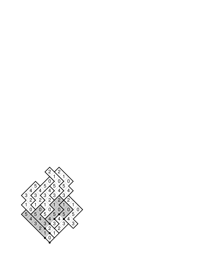
Figure 3. This path of vertices (beginning with the lowest boundary vertex) passes each shaded square on the left once.

We define $\phi(p)=\sum_{i=0}^{k-1}\phi(v_{i},v_{i+1})$ and observe the following:

Proposition 2.1.

The height function value at $v_{k}$ can be written as

$$h_{\alpha}(v_{k})=\phi(p)+\sum\phi(s),$$

where the latter sum is over all squares (counted with multiplicity) that $p$ passes on the left.

To see this, let $p^{\prime}$ be a path from $v_{0}$ to $v_{k}$ that is the same as $p$ except that each interval that crosses a tile $t$ is replaced by the path around the boundary of $t$ on the left side of $p$. The reader may easily check that $\phi(p^{\prime})-\phi(p)$ is equal to the sum of $\phi(s)$ over all squares (counted with multiplicity) that $p$ passes on the left. By definition, $h_{\alpha}(v_{k})=\phi(p^{\prime})$, so the proposition follows.

Since $\phi(p)$ is independent of the particular tiling $\alpha$, we have a simple interpretation of the height function $h_{\alpha}(v)$: it tells us the sum of $\phi(s)$ over the squares $s$ passed on the left by a path from $v_{0}$ to $v$. For our height function to be maximally informative, $G$ must be (or at least contain) the abelian group generated by $\phi(s)$ subject to only the tiling relations. We refer to this group as the canonical abelian height space (also known as the color group) of a set of tiles $T$.

We say two squares $s_{1}$ and $s_{2}$ have the same color if it can be deduced from the tiling relations that $\phi(s_{1})=\phi(s_{2})$. (In other words, $s_{1}-s_{2}$ is zero in the group generated by the squares of $\mathbb{Z}^{2}$ modulo the relations $\sum_{s\in t}s=0$ for all $t\in T$.)

This notion is best illustrated using our primary example: ribbon tiling. Let $s_{x,y}$ denote the square at position $(x,y)$ in the lattice, and consider two overlapping horizontal ribbon tiles of length $n$, one of which has leftmost square $s_{x,y}$ and the other $s_{x+1,y}$. The corresponding tile relations tell us that $\sum_{i=0}^{n-1}\phi(s_{x+i,y})=0$ and $\sum_{i=1}^{n}\phi(s_{x+i,y})=0$. And this implies that $\phi(s_{x,y})=\phi(s_{x+n,y})$. Thus, $s_{x,y}$ and $s_{x+n,y}$ have the same color.

Repeating similar arguments with other pairs of ribbon tiles that overlap on all but one square, one can deduce that squares at $(x_{1},y_{1})$ and $(x_{2},y_{2})$ necessarily have the same color whenever $x_{1}+y_{1}$ and $x_{2}+y_{2}$ are equivalent modulo $n$. Denote by $e_{i}$ the value of $\phi(s_{x,y})$ when $x+y\equiv i\pmod{n}$. Then the relation $\sum_{i=0}^{n-1}e_{i}=0$ is enough to guarantee that $\phi(t)=0$ for any ribbon tile $t$ of length $n$. Thus, if $G$ is the abelian group generated by $e_{0},\ldots,e_{n-1}$ subject to this one relation, $G$ is maximally informative.

At this point, we know the value of $\phi(s)\in G$ for every square $s$. However, we still have to choose a function $\phi$ on the edges of the $\mathbb{Z}^{2}$ lattice in such a way that $\phi(s)$ has the desired values. This is essentially a linear algebra problem, and it is not hard to see that it always has at least one solution. (We return to this issue in the next section.)

This “maximally informative” abelian height function construction is unique up to two obvious transformations. First, change of basis: one can replace $G$ with any group $G^{\prime}$ and the $e_{i}$ with any elements of $G^{\prime}$ satisfying the necessary relations. Second, translation by a tiling-independent function: one can add to $\phi(e)$ any function $\phi^{\prime}$ satisfying $\phi^{\prime}(s)=0$ for all $s$. This amounts to adding a function (independently of $\alpha$) to each height function $h_{\alpha}$.

In particular applications, we try to choose the basis for $G$ and the values of $\phi$ on the edges in $\mathbb{Z}^{2}$ in a way that makes the tiling space easy to understand. In particular, if $T$ is translation invariant, it is usually convenient for $\phi$ to have some translational symmetries as well.

3. Ribbon Tilings

3.1. Height Functions for Ribbon Tilings

Although we determined in the last section that $\phi(s)=e_{i}$ when $s$ is a square of color $i$, we have considerable freedom in choosing the values of $\phi$ on the edges in $\mathbb{Z}^{2}$. We will use this freedom to force $\phi$ to have certain symmetries.

First, we would like $\phi$ to be invariant under color-preserving translations of $\mathbb{Z}^{2}$; this amounts to the requirement that $\phi(e)$ be the same whenever $e$ is a vertical (or similarly, horizontal) edge of type $(i,i+1)$ oriented with color $i+1$ on the left. We would also like $\phi$ at such an edge to have the same value—call it $e_{i,i+1}$—independently of whether the edge is horizontal or vertical.

Let $e_{0,1},e_{1,2},\ldots,e_{n-1,0}$ be basis elements of a height space $G=\mathbb{Z}^{n}$. Summing around a square of color $i$ tells us that $e_{i}$ must be equal to $2e_{i,i+1}-2e_{i-1,i}$. Since this clearly implies $\sum_{i=0}^{n}e_{i}=0$, we need not add any additional relations to $G$. (Although the canonical abelian height function space is the subgroup of $G$ generated by the values $e_{i}=2e_{i,i+1}-2e_{i-1,1}$, it will be notationally convenient to define $\phi$ and our height functions in this larger group.) We can now describe our height function $h_{\alpha}$ for a tiling $\alpha$ with the following rules:

1. Let $h_{\alpha}(v_{0})=0$ for all tilings $\alpha$ of $R$, where $v_{0}$ is a reference vertex on the boundary of $R$.

2. When moving from one vertex to a neighbor along an edge separating $i$ and $i+1$ color squares with color $i+1$ on the left, the height changes by $e_{i,i+1}$ if no tile of $\alpha$ is crossed.

3. When moving from one vertex to a neighbor along an edge separating $i$ and $i+1$ color squares with color $i+1$ on the left, the height changes by $2e_{j,j+1}-e_{i,i+1}$ if the edge crosses a tile in $\alpha$ of type $(j,j+1)$.

We write $h^{i,i+1}_{\alpha}$ to mean the $e_{i,i+1}$ component of the height function $h_{\alpha}$. Of course, there is some redundancy in using an $n$ dimensional height space instead of the canonical $n-1$ dimensional height space; as currently defined, $\sum_{i=0}^{n-1}h^{i,i+1}_{\alpha}$ is a function that does not depend on the tiling $\alpha$. In particular, if $n=2$, the projection sending $ae_{0,1}+be_{1,0}$ to the integer $a-b$ transforms our two-dimensional $h_{\alpha}$ into the standard one-dimensional domino-tiling height function without any loss of information.

3.2. Interpretations of Ribbon Tiling Height Functions

We can understand what the height function means by looking at its behavior along diagonals. We say $p$ is an $(i,i+1)$ diagonal if:

1. The path $p=v_{0},\ldots,v_{k}$ is a connected left-to-right path made solely of edges of type $(i,i+1)$ that are incident to squares in $R$.

2. Both $v_{0}$ and $v_{k}$ are on the boundary of $R$ and the extending edges $(v_{-1},v_{0})$ and $(v_{k},v_{k+1})$ of type $(i,i+1)$ are not incident to squares in $R$.

Note that as one moves from left to right along an $(i,i+1)$ diagonal, $h^{j,j+1}_{\alpha}$ increases by two if we cross a a tile of type $(j,j+1)$ and zero otherwise. Thus, in the diagonal described above, $h^{j,j+1}_{\alpha}(v_{i})$ is equal to $h^{j,j+1}_{\alpha}(v_{0})$ plus twice the total number of times the path $v_{0},\ldots,v_{i}$ crosses a tile of type $(j,j+1)$. In particular, since the value of $h_{\alpha}$ on the boundary of $R$ is independent of $\alpha$, we have the following.

Lemma 3.1.

If $j\not=i$, then the total number of tiles of type $(j,j+1)$ crossed by the portion of an $(i,i+1)$ diagonal between two consecutive boundary vertices $v_{1}$ and $v_{2}$ is equal to $\frac{1}{2}(h_{\alpha}^{j,j+1}(v_{2})-h_{\alpha}^{j,j+1}(v_{1}))$. In particular, since $v_{1}$ and $v_{2}$ are boundary vertices, this number is independent of $\alpha$.

How does $h^{i,i+1}_{\alpha}$ change along an $(i,i+1)$ diagonal? We know that moving from left to right along the diagonal, it decreases by one when we cross a tile, increases by one otherwise. Also, inspection shows that there can never be tiles crossing both of two adjacent edges on a diagonal. Thus, as one moves along the diagonal from left to right, the value of $h^{i,i+1}_{\alpha}$ alternates between sequences of decreasing steps (of length at most one) and sequences of increasing steps (of length one or more). We say $v_{a}$ is a record vertex if $a\geq 1$, and $h^{i,i+1}_{\alpha}(v_{b})<h^{i,i+1}_{\alpha}(v_{a})$ whenever $0\leq b<a$. For notational convenience, we will also consider $v_{k+1}$ (the vertex just right of the vertex $v_{k}$ along an edge of type $(i,i+1)$) to be a record vertex. (See Figure 4.)

Since each decreasing sequence in $h^{i,i+1}_{\alpha}$ along $p$ has length at most one, it is not hard to check that if $2\leq a\leq k$, then $v_{a}$ is a record vertex if and only if $h^{i,i+1}_{\alpha}(v_{a})>h^{i,i+1}_{\alpha}(v_{a-1})>h^{i,i+1}_{\alpha}(v_{a-2})$. Note that the first edge $(v_{0},v_{1})$ and last edge $(v_{k-1},v_{k})$ of a diagonal are always boundary edges of $R$, and hence represent increasing steps. In particular, $v_{1}$ is always a record vertex.

What does it mean for $v_{a}$ to be a record vertex? First of all, it means that the two adjacent edges $(v_{a-2},v_{a-1})$ and $(v_{a-1},v_{a})$ are both not crossed by tiles; this in turn implies that the square $s$ incident to both of them (which we will call a record square) is either a square outside of $R$ or a square in $R$ belonging to a tile of type $(i,i+1)$. Since each of the integers $h^{i,i+1}_{\alpha}(v_{0})+1,h^{i,i+1}_{\alpha}(v_{0})+2,\ldots,h^{i,i+1}_{\alpha}(v_{k})$ must occur as a record value exactly once, the number of record vertices on the diagonal (not counting $v_{k+1}$) is equal to $h^{i,i+1}_{\alpha}(v_{k})-h^{i,i+1}_{\alpha}(v_{0})$, and is hence independent of $\alpha$.

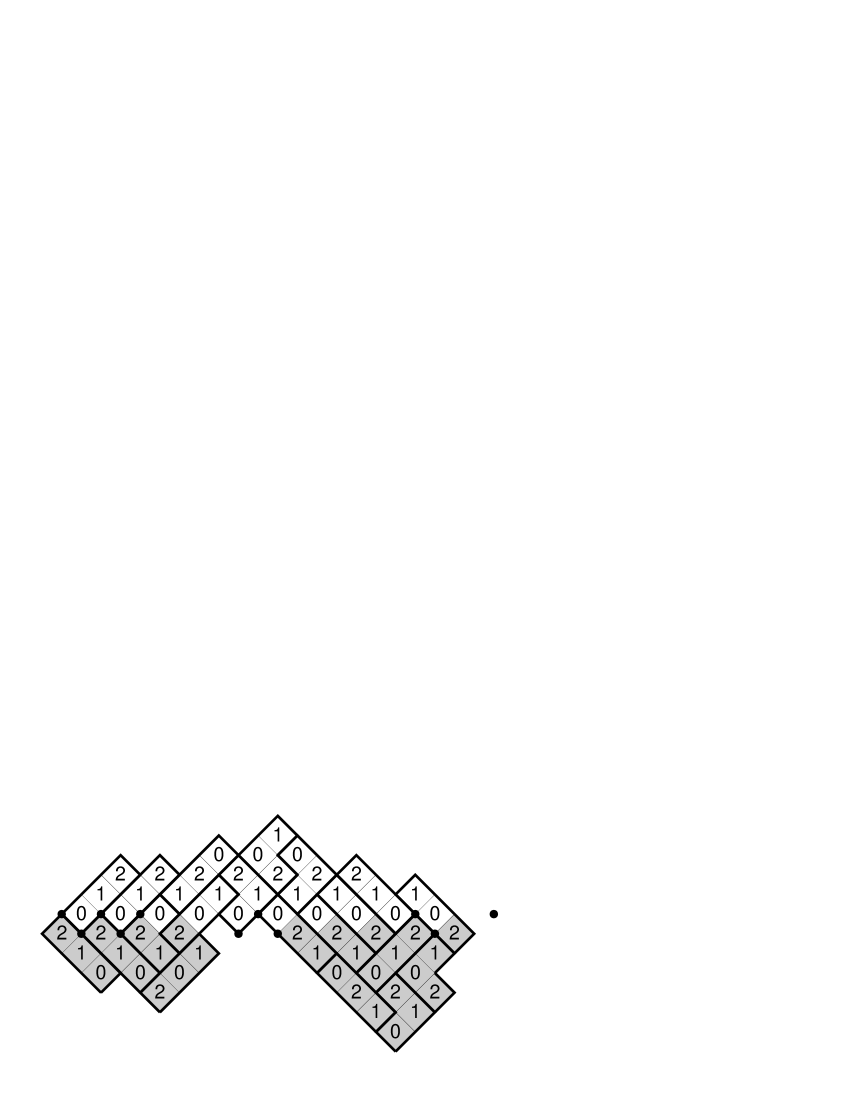
Figure 4. Let $p$ be the diagonal of type $(2,0)$ that separates the shaded squares from the unshaded squares. If $v_{0}$ is the leftmost corner of the figure, then $h^{2,0}_{\alpha}(v_{0})=0$. As one moves from left to right along the diagonal, $h^{2,0}_{\alpha}$ assumes, in order, the values $0,1,2,3,4,5,4,5,4,5,6,7,8,7,8,7,8,7,8,9,10,9,10$. The dots indicate record vertices—one for the first occurrence of each number between $1$ and $10$ and one for the first vertex outside of $R$; the square immediately left of each record vertex is either a boundary square or a square in a tile of type $(2,0)$. The relation $\prec$ induces a total ordering on this set of four boundary squares and seven type $(2,0)$ tiles. Every pair of elements in this set corresponds to a forced edge of $G_{R}(\alpha)$.

Now, if $s$ is a record square outside of $R$ and $v_{a}$ is the corresponding record vertex, the two diagonal edges preceding $v_{a}$ must both be boundary edges of $R$ (unless one is an edge outside of $R$); hence, $s$ will be a record square for every tiling of $R$. If $a\neq k+1$, then the value $h_{\alpha}(v_{a})$ is also independent of the tiling. Whenever $s$ is a record square outside of $R$, the corresponding record vertex is called a boundary record vertex; in particular, $v_{1}$ and $v_{k+1}$ are boundary record vertices.

Between any two consecutive boundary record vertices $v_{a}$ and $v_{b}$, there are exactly $h^{i,i+1}_{\alpha}(v_{b})-h^{i,i+1}_{\alpha}(v_{a})-1$ record vertices whose record squares are squares of tiles of type $(i,i+1)$. Whether the tile lies above or below the diagonal clearly depends on the parity of $a$; since $h^{i,i+1}$ alternates parity along the diagonal, this in turn depends on the parity of the $h^{i,i+1}_{\alpha}$ at the record vertex $v_{a}$. We call $v$ a lower record vertex if the corresponding record square lies below the diagonal and an upper record vertex if it lies above the diagonal. Since for each $\alpha$, the record values $h^{i,i+1}_{\alpha}(v_{0})+1,h^{i,i+1}_{\alpha}(v_{0})+2,\ldots,h^{i,i+1}_{\alpha}(v_{k})$ must be attained in the same order, we have the following lemma:

Lemma 3.2.

Suppose $q$ is the portion of a diagonal $p$ of type $(i,i+1)$ between two consecutive boundary record vertices $v_{a}$ and $v_{b}$. Then the number tiles of type $(i,i+1)$ with squares adjacent to $q$ that lie above or below the diagonal is equal to $h^{i,i+1}_{\alpha}(v_{b})-h^{i,i+1}_{\alpha}(v_{a})-1$. In particular, this value is the same for every tiling of $R$. Furthermore, the order in which the entire diagonal $p$ encounters boundary record vertices, lower record vertices, and upper record vertices is also the same for every tiling of $R$ and can be determined from the value of the height function on the boundary vertices in $p$.

Denote by $S_{\alpha}(p)$ the set of squares adjacent to $p$ that are either members of tiles of type $(i,i+1)$ or squares in $B_{R}$. (See Figure 4.) Note that if $s_{1}$ and $s_{2}$ are two record squares then $s_{1}\prec s_{2}$ if and only if the record vertex for $s_{1}$ occurs before that of $s_{2}$ in the diagonal. Thus, we can restate the previous lemma:

Lemma 3.3.

Given any two tilings $\alpha$ and $\alpha^{\prime}$, $S_{\alpha}(p)$ and $S_{\alpha^{\prime}}(p)$ contain the same number of boundary squares, squares of color $i$ in type $(i,i+1)$ tiles, and squares of color $i+1$ in type $(i,i+1)$ tiles. The relation $\prec$ induces a total ordering on the squares in $S_{\alpha}(p)$ as well as those in $S_{\alpha^{\prime}}(p)$; if the $m$th square in the ordering of $S_{\alpha}(p)$ is a boundary square (or a square of color $i$ in a type $(i,i+1)$ tile, or a square of color $i+1$ in a type $(i,i+1)$ tile), the same is true of $S_{\alpha^{\prime}}(p)$.

Now we are ready to prove Lemma 1.2, which we restate here for convenience.

Lemma 3.4.

Any two tilings $\alpha$ and $\beta$ of $R$ necessarily contain the same number of tiles of each level. Thus, $t_{c,i}(\alpha)$ is defined if and only if $t_{c,i}(\beta)$ is defined. Furthermore, if $c\equiv d\pmod{n}$, then $t_{c,i}(\alpha)\prec t_{d,j}(\alpha)$ if and only if $t_{c,i}(\beta)\prec t_{d,j}(\beta)$. Also, if $b\in B_{R}$, then $t_{c,i}(\alpha)\prec b$ if and only if $t_{c,i}(\beta)\prec b$ . Similarly, $b\prec t_{c,i}(\alpha)$ if and only if $b\prec t_{c,i}(\beta)$.

Proof.

Let $t_{c,1}(\alpha)\prec t_{c,2}(\alpha)\prec\ldots\prec t_{c,k}(\alpha)$ be the tiles of type $(i,i+1)$ in $\alpha$ whose lowest squares lie just above a given diagonal $p$. It is obvious from the definition of $t_{c,i}(\alpha)$ that the ordering of these tiles with respect to each other is independent of $\alpha$. Similarly, let $t_{c-n,1}(\alpha)\prec t_{c-n,2}(\alpha)\prec\ldots\prec t_{c-n,m}(\alpha)$ be the tiles of type $(i,i+1)$ that lie just below the diagonal $p$.

Now, let $a_{1}\prec a_{2}\prec\ldots\prec a_{r}$ be the totally ordered set of all the boundary squares and all of the $k+m$ tiles that are incident to $p$. Since we know that the ordering restricted to the set of tiles of form $t_{c,i}(\alpha)$ (or the set of tiles of form $t_{c-n,i}(\alpha)$, or the set of boundary squares) is independent of $\alpha$, it follows from Lemma 3.3 that the total ordering $a_{1}\prec a_{2}\prec\ldots\prec a_{r}$ is independent of $\alpha$.

Since any two tiles of the same type or any tile and any square that are comparable by $\prec$ must be incident to some common diagonal $p$, Lemma 3.3 covers all possible cases in which the $\prec$ relation occurs between tiles of the same type or between tiles and boundary squares. ∎

The reader may recall from the introduction that we used this lemma used to define the partially oriented graph $G_{R}$ and to justify our interpretation of $G_{R}{\alpha}$ as an extension of the partial orientation of $G_{R}$. This will be the topic of the next section.

3.3. The Acyclic Orientation Correspondence

The purpose of this section is to prove Theorem 1.3; we will state and prove each of its four parts as a separate lemma.

Lemma 3.5.

For every order-$n$ ribbon tiling $\alpha$ of $R$, $G_{R}(\alpha)$ is an acyclic orientation extending the partial orientation of $G_{R}$.

Proof.

We must show that, given a tiling $\alpha$, there exists no sequence

$$a_{0}\prec a_{1}\prec a_{2}\prec\ldots\prec a_{k}\prec a_{0},$$

where each $a_{i}$ is either a tile or a square in $B_{R}$.

Since there can clearly be no cycle containing one or two elements, we may assume $k\geq 2$. Now, suppose a diagonal incident to both $a_{0}$ and $a_{k}$ is also incident to some $a_{i}$ with $0<i<k$. If $a_{k}\prec a_{i}$, then $a_{i}\prec a_{i+1}\prec\ldots\prec a_{k}\prec a_{i}$ is a shorter cycle. If $a_{i}\prec a_{k}$, then $a_{i}\prec a_{0}$ (by transitivity, since $a_{i}$, $a_{k}$, and $a_{0}$ are on the same diagonal and hence totally ordered), and $a_{0}\prec a_{1}\prec\ldots\prec a_{i}\prec a_{0}$ is a shorter cycle.

Thus, if $a_{0}\prec a_{1}\prec a_{2}\prec\ldots\prec a_{k}\prec a_{0}$ is a cycle of minimal length in $G_{R}(\alpha)$, then any infinite diagonal that is incident to both $a_{0}$ and $a_{k}$ can be incident to no other tile or square. Denote by $p_{z}$ the infinite diagonal between square levels $z$ and $z+1$ and let $z^{\prime}$ and $z^{\prime\prime}$ be the lowest and highest values of $z$ for which $p_{z}$ is incident to both $a_{0}$ and $a_{k}$. All tiles and squares other than $a_{0}$ and $a_{k}$ must lie entirely below $p_{z^{\prime}}$ or entirely above $p_{z^{\prime\prime}}$. Since no tile or square below $p_{z^{\prime}}$ can be comparable with any tile or square above $p_{z^{\prime\prime}}$, the sequence $a_{1}\prec a_{2}\prec\ldots\prec a_{k-1}$ must lie entirely above $p_{z^{\prime\prime}}$ or entirely below $p_{z^{\prime}}$. Suppose without loss of generality that the former is the case and that the lowest square in $a_{0}$ is at least as low as the lowest square in $a_{k}$. Then none of the elements $a_{i}$ below $p_{z^{\prime}}$ is comparable with $a_{k}$, and this is a contradiction. ∎

Lemma 3.6.

If $\alpha$ and $\beta$ are order-$n$ ribbon tilings then $\alpha=\beta$ if and only if $G_{R}(\alpha)=G_{R}(\beta)$.

Proof.

Obviously, the first statement implies the second. Now, suppose $G_{R}(\alpha)=G_{R}(\beta)$. Since these orientations are acyclic, there must exist at least one leftmost tile, i.e., there exists a $t_{c,i}$ for which there exists no $t_{d,j}$ with $t_{d,j}(\alpha)\prec t_{c,i}(\alpha)$ or $t_{d,j}(\beta)\prec t_{c,i}(\beta)$. It follows that $t_{c,i}(\alpha)$ and $t_{c,i}(\beta)$ must each contain the leftmost squares in $R$ in the rows of level $c,c+1,\ldots,c+n-1$; thus, their positions are determined and they are equal. Similarly, we can now choose a $t_{d,j}$ that is leftmost among the remaining set of tiles, and its position is also completely determined. Repeating this argument, we conclude that $t_{c,i}(\alpha)=t_{c,i}(\beta)$ for all $c$ and $i$ for which these values are defined. ∎

Lemma 3.7.

Every acyclic orientation $A$ of $G_{R}$ that extends the partial orientation of $G_{R}$ can be written as $G_{R}(\alpha)$ for some tiling $\alpha$.

In the introduction, we defined $G_{R}$ by assuming that $R$ admitted at least one tiling $\alpha$ and restricting the orientation on $G_{R}(\alpha)$ to the forced edges. However, in our later existence proofs, it will be necessary to have a definition of $G_{R}$ and a version of Lemma 3.7 that do not invoke a priori knowledge of the existence of $\alpha$. To do this, we will need some definitions.

We say a tile vertex $t_{c,i}$ crosses level $d$ if $c\leq d\leq c+n-1$. (Note that if $\alpha$ is a tiling, then $t_{c,i}$ crosses level $d$ if and only if $t_{c,i}(\alpha)$ contains a square of level $d$.) We define a partially oriented graph $G$ to be a ribbon tile graph consistent with $R$ if the following hold:

1. The vertices of $G$ come from the set of tile vertices $t_{c,i}$ (with $c,i\in\mathbb{Z}$ and $i>0$) and square vertices $s_{x,y}$ (with $x,y\in\mathbb{Z}$).

2. Two tile vertices $t_{c,i}$ and $t_{d,j}$ are adjacent if and only if $|c-d|\leq n$. A tile $t_{c,i}$ and square $s_{x,y}$ are adjacent if and only if $c-1\leq x+y\leq c+n$. Two squares $s_{x,y}$ and $s_{x^{\prime},y^{\prime}}$ are adjacent if and only if $|(x+y)-(x^{\prime}+y^{\prime})|\leq 1$.

3. The graph $G$ is endowed with an orientation on its forced edges (i.e. all edges involving a square or involving two tile vertices $t_{c,i}$ and $t_{d,j}$ with $c\equiv d\pmod{n}$). No other edges of $G$ are oriented.

4. If $s_{1}$ and $s_{2}$ are square vertices, then the edge $(s_{1},s_{2})$ is oriented toward $s_{2}$ if and only if $s_{1}\prec s_{2}$. Also, whenever $i>0$ and $t_{c,i+1}$ is a tile vertex, $t_{c,i}$ is also a tile vertex. An edge of the form $(t_{c,i},t_{c,j})$ is oriented toward $t_{c,j}$ whenever $i<j$.

5. The set of square vertices of $G$ is precisely the set of boundary squares of $R$.

6. The total number of tiles crossing a given level $c$ is precisely the number of squares in $R$ of level $c$.

7. For every integer $c$ and every pair of boundary squares $b_{1}$ and $b_{2}$ of levels $c-1$, $c$, or $c+1$ satisfying $b_{1}\prec b_{2}$, the number of tile vertices $t_{d,j}$ in $G_{R}$ that cross level $c$ and satisfy $b_{1}\prec t_{d,j}\prec b_{2}$ is precisely the number of squares $s$ in $R$ of level $c$ satisfying $b_{1}\prec s\prec b_{2}$.

Only the last three conditions depend on $R$; we will refer to these as the consistency conditions. Although it involves overloading the symbol $\prec$, we will write $a\prec b$ whenever the edge $(a,b)$ is a forced edge of $G$ oriented toward $b$. If $A$ is an orientation extending the partial orientation on the forced edges of $G$, we write $a\prec_{A}b$ if the edge $(a,b)$ in $G$ is oriented from $a$ to $b$ in $A$.

Note that up to this point, we have defined $\prec$ only on actual tiles, not on the tile vertices $t_{c,i}$, which are abstract place holders for tiles. However, our expanded use of $\prec$ is consistent in the following sense: if $G_{R}(\alpha)$ is the ribbon tiling graph of a tiling $\alpha$ and the edge $(t_{c,i},t_{d,j})$ is forced, then $t_{c,i}(\alpha)\prec t_{d,j}(\beta)$ if and only if $t_{c,i}\prec t_{d,j}$ in $G_{R}$. Similarly, if $A=G_{R}(\alpha)$ and the edge is $(t_{c,i},t_{d,j})$ is not necessarily forced, then $t_{c,i}(\alpha)\prec t_{d,j}(\alpha)$ if and only if $t_{c,i}\prec_{A}t_{d,j}$. Similar results apply to edges involving squares.

If $R$ admits a tiling $\alpha$ then the graph $G_{R}$ as defined in the introduction clearly satisfies the above list of requirements and is consistent with $R$. (In fact, $G_{R}$ is the only ribbon tile graph consistent with $R$ in this case.) Thus, the following is a slightly more general version of Lemma 3.7:

Lemma 3.8.

Suppose $G_{R}$ is any ribbon tile graph that is consistent with $R$. Then every acyclic orientation $A$ of $G_{R}$ that extends the partial orientation on the forced edges of $G_{R}$ is equal to $G_{R}(\alpha)$ for some tiling $\alpha$. (In particular, if $R$ does not admit an order-$n$ ribbon tiling, then no such $G_{R}$ and $A$ exist.)

Proof.

Suppose $t=t_{c,1}$ is a leftmost tile vertex in $G_{R}$. As in the previous proof, we will choose the leftmost squares of each of the levels $c,c+1,\ldots,c+n-1$ and declare them to be our first tile $t_{c,1}(\alpha)$. That there exists at least one square in $R$ on each of these levels follows from the consistency conditions of $G_{R}$. However, we must verify that this set of squares is actually a ribbon tile. Since it contains one square on each of levels $c,c+1,\ldots,c+n-1$, it is sufficient to show that it is connected.

Suppose otherwise; then we can assume without loss of generality that there exists some $i$ such that the leftmost square $s_{i}$ in the row of level $c+i$ is left of the square $s_{i+1}$ in the row of level $c+i+1$ but that these two squares are not adjacent. Now, let $s_{r}$ ($s_{l}$) be the square of level $c+i+1$ that is right of (left of) and adjacent to $s_{i}$. Both $s_{r}$ and $s_{l}$ must be squares in $B_{R}$, since they are adjacent to $s_{i}$ and they are left of $s_{i+1}$, the leftmost square of their level in $R$.

Now, by the consistency conditions, there is exactly one tile $t^{\prime}$ containing a square on level $c+i$ such that $s_{l}\prec t^{\prime}\prec s_{r}$; every other tile with a square on level $c+i$ must be right of $s_{r}$. If $t\not=t^{\prime}$, then $t^{\prime}\prec s_{r}\prec t\prec t^{\prime}$, violating acyclicity. Hence $t=t^{\prime}$. However, since $s_{r}$ is left of every square of level $c+i+1$, one may deduce from the consistency conditions that every tile vertex $t$ of $G_{R}$ that crosses level $c+i+1$ must satisfy $s_{r}\prec t$. Thus $t\prec s_{r}\prec t$, a contradiction, and it follows that the squares chosen do in fact form a tile.

Now we form a new region $R^{\prime}$ by removing the squares in this tile from $R$. We form a new graph $G_{R^{\prime}}$ by removing $t_{c,1}$ from the vertex set of $G_{R}$—along with all boundary squares of $R$ that are not boundary squares of $R^{\prime}$—and adding all the boundary squares of $R^{\prime}$ that were not boundary squares of $R$. (These are necessarily members of our removed tile.) We define the edges of $G_{R^{\prime}}$ and their orientations in a new orientation $A^{\prime}$ in the most natural possible way. Two vertices of $G_{R^{\prime}}$ are adjacent whenever the corresponding edges in $G_{R}$ were adjacent, and $A^{\prime}$ is the orientation induced by $A$ on such edges. Furthermore, if $s$ is one of the new boundary squares and is in a row $c$, we declare it to be adjacent in $G_{R^{\prime}}$ to every tile $t$ that crosses rows $c-1$, $c$, or $c+1$ (with $s\prec t$) and every boundary square $s_{0}$ of those levels (with $s\prec s_{0}$ if and only if $s$ is directly or indirectly left of $s_{0}$ and $s_{0}\prec s$ when the opposite is true). Finally, if $t_{c,j}$ was a vertex of $G_{R}$ with $j>1$, we relabel it $t_{c,j-1}$ in $G_{R^{\prime}}$.

It follows easily from the definition that the $G_{R^{\prime}}$ thus defined—together with the partial orientation on forced edges induced by $A^{\prime}$—is a ribbon tile graph consistent with $R^{\prime}$. If we can further prove that $A^{\prime}$ is necessarily acyclic, then Lemma 3.8 will follow by induction.

Suppose $A^{\prime}$ has a cycle; then this cycle must include a square $s$ of $B_{R^{\prime}}$ that was a member of the tile $t$—otherwise the cycle would also be a cycle in $A$. Also, although the cycle may contain multiple squares from the removed tile, it must contain at least one element that is not a square of $t$, since the squares do not themselves contain any cycles. Suppose the cycle contains a sequence $s_{1}\prec\ldots\prec s_{k}$ of former squares of $t$ but that the elements $a$ immediately preceding this sequence and $b$ immediately following it are not squares of $t$. Then we must have had $a\prec t\prec b$ in $A$, and $A$ too must have had a cycle. ∎

Lemma 3.9.

Two order-$n$ ribbon tilings $\alpha$ and $\beta$ differ by a local replacement move if and only if $G_{R}(\alpha)$ and $G_{R}(\beta)$ differ by an edge reversal.

Figure 5. Two examples of local replacement moves

Proof.

First of all, we can determine whether a local replacement move involving tiles $t_{c,i}(\alpha)$ and $t_{d,j}(\alpha)$ can occur by applying the theory we have already developed to $R^{\prime}$, the region tiled by just these two tiles. Now, if $R^{\prime}$ admits two distinct tilings, then $G_{R^{\prime}}$ must admit two distinct orientations that extend the orientation on the forced edges. In particular, $G_{R^{\prime}}$ must contain at least one free edge, and that can only be the edge $(t_{c,i},t_{d,j})$. For this edge to be free, we must have $0<|c-d|<n$.

Without loss of generality, suppose $c<d$. Notice that if $d\leq e\leq c+n-1$, then $R^{\prime}$ contains two squares of level $e$. Inspection shows that if tile $t_{c,i}(\alpha)$ contains the leftmost square of one of these same-level pairs, it must contain the leftmost square of every such pair. (See Figure 5.) Moreover, if a tile contains one square on a row higher than $c+n-1$ (lower than $d$), it must contain every square with this property. Thus, a local replacement move must consist of swapping the squares in each same-level pair. Such a swap produces a new pair of ribbon tiles if and only if the single square on row $d-1$ (resp., $c+n$) is adjacent to both of the squares in row $d$ (resp., $c+n-1$). Inspection shows that whenever there is no square $s$ with either $t_{c,i}(\alpha)\prec s\prec t_{d,j}(\alpha)$ or $t_{d,j}(\alpha)\prec s\prec t_{c,i}(\alpha)$, then a local move can in fact occur.

Now, if $\beta$ is the tiling obtained by applying such a move to $\alpha$, and $t_{c,i}(\alpha)\prec t_{d,j}(\alpha)$ then inspection shows that we must have $t_{d,j}(\beta)\prec t_{c,i}(\beta)$; it is also easy check that if $a$ is any tile or square outside of $R^{\prime}$, then $a\prec t_{c,i}(\alpha)$ if and only if $a\prec t_{c,i}(\beta)$. Similarly, $t_{c,i}(\alpha)\prec a$ if and only if $t_{c,i}(\beta)\prec a$. It follows that if $\alpha$ and $\beta$ differ by a local replacement move, $G_{R}(\alpha)$ and $G_{R}(\beta)$ do in fact differ by the reversal of exactly one edge: the edge $(t_{c,i},t_{d,j})$.

For the converse, note that if the orientation of an edge $(t_{c,i},t_{d,j})$ of the orientation $G_{R}(\alpha)$ can be reversed without creating a cycle, we know there must be no vertex $a$ of $G_{R}(\alpha)$ with either $t_{c,i}(\alpha)\prec a\prec t_{d,j}(\alpha)$ or $t_{d,j}(\alpha)\prec a\prec t_{c,i}(\alpha)$; we have already shown that this is a sufficient condition for there to exist a local move involving the tiles $t_{c,i}(\alpha)$ and $t_{d,j}(\alpha)$, and so $G_{R}(\beta)$ must be the orientation obtained by reversing the edge. ∎

3.4. The Existence Algorithm

The main result of this section will be a linear-time algorithm for determining whether a simply connected region $R$ has an order-$n$ ribbon tiling and constructing such a tiling when one exists. To determine existence, we will make use of the well-known fact (which we later prove) that there exists an acyclic orientation $A$ of a graph $G$ that extends a given partial orientation of $G$ if and only if the partial orientation is itself acyclic. This implies the following corollary of Lemma 3.8:

Corollary 3.10.

Given $R$, there exists an acyclic partially oriented ribbon tiling graph $G_{R}$ that is consistent with $R$ if and only if $R$ admits an order-$n$ ribbon tiling.

Using this fact, we divide our algorithm into three steps.

1. We either produce an acyclic ribbon tile graph $G_{R}$ that is consistent with $R$ or prove that no such graph exists (and hence $R$ admits no order-$n$ ribbon tiling).

2. If we succeed in producing $G_{R}$ in the previous step, we describe a total ordering on the vertices of $G_{R}$ that induces the partial orientation of $G_{R}$ on the forced edges of $G_{R}$.

3. Given this totally ordering on the vertices of $G_{R}$, we describe a tiling of $R$.

Now, we know that if there is an acyclic ribbon tile graph $G_{R}$ that is consistent with $R$, we can use it to generate $G_{R}(\alpha)$ using the construction of Lemma 3.8, and the partial orientation on $G_{R}$ will thus be the restriction of $G_{R}(\alpha)$ to the forced edges in $G_{R}$. Thus, in the construction that follows, we can make use of lemmas proved earlier in the paper under the assumption that $R$ had a tiling. If $R$ does have a tiling, our assumption will have been correct. If $R$ does not have a tiling, these assumptions will lead to contradictions, and these will enable us to conclude that no tiling exists.

Now we begin to construct $G_{R}$. Let $S(c)$ be the number of squares of level $c$ and let $T(c)$ be the number of tiles whose lowest square is $c$. Clearly $T(c)=S(c)-\sum_{i=1}^{n-1}T(c-i)$, and is thus easily computed for each $c$ in linear time. (If it is not the case that $T(c)\geq 0$ whenever $S(c)\not=0$ and $T(c)=0$ whenever $S(c)=0$, we can conclude that no tiling exists.) For each $c$ for which $T(c)\not=0$, we include $t_{c,i}$ for $1\leq i\leq T(c)$ as tile vertices of $G_{R}$. We also include all the boundary squares of $R$ as square vertices of $G_{R}$. This $G_{R}$ has an edge whenever the corresponding tiles/squares are on levels that would make them comparable by $\prec$, and we require that $t_{c,i}\prec t_{c,i+1}$ whenever both of these vertices are in $G_{R}$.

We would now like to determine an orientation on the forced edges of $G_{R}$ that will make $G_{R}$ a consistent ribbon tiling graph. We will not store in memory all of the edges of $G_{R}$ (as the number of such edges could be quadratic in the size of $R$); instead, we will observe that the partial orientation on $G_{R}$ induces a total ordering $a_{0}\prec a_{1}\prec\ldots\prec a_{k}$ on the set of squares and tiles of a given type that are all incident to a common diagonal. Since every forced edge can be derived from such an ordering on some diagonal, it will thus be sufficient for us to store in memory the actual orderings corresponding to each such type/diagonal pair, and this requires only a linear amount of memory.

Given an infinite diagonal $p$ between square rows of levels $c-1$ and $c$ and some $j\in\{1,2,\ldots,n-1\}$, let $\mathcal{S}_{j,p}$ be the set of tiles in $G_{R}$ of the form $t_{c-j,i}$ together with squares in $G_{R}$ on levels $c-1$ and $c$. Since the elements in $S_{j,p}$ share a common diagonal and all tiles in this set are of the same type, each pair of elements in $S_{j,p}$ is connected by a forced edge and hence $G_{R}$ induces a total ordering on this set. Now, we can compute the height function $h$ on the boundary of $R$, and using $h$, we can deduce this ordering explicitly from Lemma 3.1 as follows. Let $k=c-j-1\pmod{n}$. Given consecutive boundary vertices $v_{1}$ and $v_{2}$ along the diagonal, we know that the number of tiles of the form $t_{c-j,i}$ (and hence of type $(k,k+1)$) that cross $p$ between consecutive boundary vertices $v_{1}$ and $v_{2}$ must be $\frac{1}{2}(h^{k,k+1}(v_{2})-h^{k,k+1}(v_{1}))$. Clearly, if $b_{1}$ is a square incident to the diagonal $p$ immediately before $v_{1}$ and $b_{2}$ is a square incident to $p$ immediately after $v_{2}$, the number of tiles $t$ of the form $t_{c-j,i}$ satisfying $b_{1}\prec t\prec b_{2}$ must be exactly $\frac{1}{2}(h^{k,k+1}(v_{2})-h^{k,k+1}(v_{1}))$. Thus, we can compute the number of tiles of $S_{j,p}$ in between each pair of boundary squares, and this completely determines the ordering.

Similarly, given an infinite diagonal $p$ between square rows $c-1$ and $c$, let $\mathcal{S}_{p,0}$ be the set of tiles in $G_{R}$ of the form $t_{c,i}$ or $t_{c-n,i}$ together with the squares in $G_{R}$ on levels $c-1$ and $c$. Each pair of elements in $\mathcal{S}_{p,0}$ is connected by a forced edge, and thus the partial orientation on $G_{R}$ must induce a total ordering on this set. By Lemma 3.2 and Lemma 3.3, we can deduce this total ordering from the value of the height function on the boundary vertices of $R$ in $p$.

Since every forced edge involves two elements along the same diagonal, we can compute the orientation of each forced edge by repeating this process for each diagonal. Now we check that if $G_{R}$ is acyclic, it is necessarily a consistent ribbon tiling graph. It is enough to check the consistency conditions. By construction, $G_{R}$ contains all boundary squares, and by the definition of $T(c)$, the total number of tiles crossing each level $c$ is the number of squares in $R$ of level $c$. For the final consistency condition, suppose $c$ is given and $b_{1}$ and $b_{2}$ are boundary squares of types $c-1$, $c$, or $c+1$ with $b_{1}\prec b_{2}$.

Then let $p_{1}$ be the diagonal above the row of squares of level $c$ and let $p_{2}$ the diagonal below these squares. One easily checks that both $p_{1}$ and $p_{2}$ contain edges in each of $b_{1}$ and $b_{2}$. It suffices to check the condition under the assumption that there exists no boundary square $b_{3}$ incident to $p$ with $b_{1}\prec b_{3}\prec b_{2}$, since otherwise we can check the condition separately for the pair $(b_{1},b_{3})$ and the pair $(b_{3},b_{2})$. Say a vertex has level $c$ if it is a corner of squares of type $c-1$, $c$, and $c+1$, and let $q$ be the portion of the diagonal connecting the last level $c$ vertex of $b_{1}$ to the first level $c$ vertex of $b_{2}$.

Then it follows by applying Lemma 3.1 to the diagonal $p_{1}$ (or to $p_{2}$ if $p_{1}$ has type $(j,j+1)$) that the number of tile vertices $t$ of type $(j,j+1)$ crossing $c$ and satisfying $b_{1}\prec t\prec b_{2}$ must be equal to $\frac{1}{2}(h^{j,j+1}(v_{2})-h^{j,j+1}(v_{1}))$. Write $\overline{h}=\sum_{j=0}^{n-1}h^{j,j+1}$, and note that the total number of such tile vertices must then be $\frac{1}{2}(\overline{h}(v_{2})-\overline{h}(v_{1}))$. However, this function is tiling-independent and in fact always increases by one as we move between squares of color $j$ and $j+1$ with $j+1$ on the left. It follows that if the vertices of the grid are labeled with coordinates $(u,v)$, then $\overline{h}(u,v)$ will be equal to $u-v$ plus a constant. In particular, this implies that $\frac{1}{2}(\overline{h}(v_{2})-\overline{h}(v_{1}))$ is equal to the number of squares on level $c$ directly between vertices $v_{1}$ and $v_{2}$, and this is easily seen to be the number of level $c$ squares $s$ in $R$ satisfying $b_{1}\prec s\prec b_{2}$.

Figure 6. A graphical representation of $G_{R}$ when $n=3$ and $R$ is the $9\times 9$ grid. Each of the dots represents one of the $27$ tile vertices of $G_{R}$ (square vertices are not shown), and the $15$ horizontal lines correspond to the $15$ levels on which tiles occur. All essential forced edges between tiles of the same type are shown with orientations. Two vertices in this figure are adjacent in $G_{R}$ if and only if the difference between their levels is at most three.

The only remaining step is to determine whether our partial orientation of $G_{R}$ is indeed acyclic. There are many of ways to do this in time linear in the number of edges of $G_{R}$. We say a forced edge $(a,b)$ of $G_{R}$ is essential if $a\prec b$ and there exist no forced edges $(a,c)$ and $(c,b)$ with $a\prec c$ and $c\prec b$—one easily checks that the number of essential forced edges of $G_{R}$ is linear in the size of $R$ and that any acyclic orientation of $G_{R}$ that extends the partial orientation on the essential forced edges must extend the partial orientation on all forced edges. (See Figure 6.) The following algorithm for determining acyclicity (know as the topological sort) is well-known, and we will apply it to the graph formed by the vertices of $G_{R}$ and the essential forced edges of $G_{R}$.

Choose a starting vertex $a_{0}$ from the set of vertices of $G_{R}$ and attempt to construct an increasing path $a_{0}\prec a_{1}\prec a_{2}\ldots$ until we either reach a point we have already visited (and we declare that there exists a cycle) or we reach a vertex $a_{k}$ that is not left of any of its neighbors. Clearly, $a_{k}$ cannot be part of a cycle, so we remove it and begin searching again with $a_{k-1}$ (if $k=0$, we choose a new $a_{0}$ arbitrarily from among the remaining vertices of $V$). We continue this process until we have removed all the vertices of $V$ or we have found a cycle.

In the former case, if we list the elements of $V$ in the order in which they were removed from $V$, we have some ordering $a_{0},a_{1},a_{2},\ldots,a_{k}$ in which $i<j$ implies $a_{i}\not\prec a_{j}$ (since $a_{i}$ could otherwise not have been removed before $a_{j}$). Thus, we can define an acyclic orientation $A$ on $G_{R}$ by simply saying that whenever $(a_{i},a_{j})$ is an edge in $G_{R}$, $a_{j}\prec_{A}a_{i}$. Let $\alpha$ be the tiling for which $G_{R}(\alpha)=A$. Then if $t_{c,i}$ is the last tile that occurs in our ordering, we know that $t_{c,i}(\alpha)$ contains the leftmost squares of rows $c,c+1,\ldots,c+n-1$. We know that the next to last tile $t_{d,j}(\alpha)$ contains the leftmost remaining squares of rows $d,d+1,\ldots,d+n-1$, and so forth. Thus, given our ordering, it is easy to explicitly determine all the tiles of $\alpha$ in linear time. Note also that this algorithm yields an explicit proof of the fact (mentioned earlier) that every acyclic partial ordering of a graph has an acyclic extension.

4. General Tilings And Abelian Height-Functions

4.1. Examples

The constructions in this paper allow us in principle to work out the maximally informative abelian height function for any polyomino tiling problem. The following facts, for example, are simple to verify:

1. Given any coloring of the squares of $R$, a generalized ribbon tiling is a tiling in which each tile contains exactly one square of each color. Suppose, for example, we color the square at position $(x,y)$ one of $mn$ colors according to the values of $x\pmod{m}$ and $y\pmod{n}$. In this case, the canonical abelian height space is $\mathbb{Z}^{mn-1}$. (When $m=n=2$, this is the square/skew-tetromino tiling problem mentioned in [17].)

2. Let $T$ be the set of all polyominos with two black and two white squares in the usual chess board coloring. (These are squares, skew-tetrominos, and length-four vertical and horizontal bars.) The canonical abelian height function space is $\mathbb{Z}\times\mathbb{Z}/2\mathbb{Z}$.

3. If $T$ contains all trominos, then the canonical abelian height space is trivial.

4. Let $T$ be the set of all rectangular $m\times 1$ tiles and $1\times n$ tiles. Then the canonical abelian height space is $\mathbb{Z}^{(m-1)(n-1)}$. (This problem was studied in [9], where connectedness under local moves was proved using a non-abelian height function.)

5. If $T$ contains only horizontal dominos, then the canonical abelian height space is infinite dimensional.

4.2. Defining height functions at all vertices

In general, the height function $h_{\alpha}$ is only defined at the vertices of $R$ that are on the boundary of tiles of $\alpha$. One (admittedly awkward) way around this is to replace each tile with a spanning tree of the squares in that tile, and consider an edge in $t$ to be on the boundary if the squares it divides are not adjacent as members of the tree. (See Figure 7.) That is, if $v_{1}$ and $v_{2}$ are adjacent vertices in $R$, we say $h_{\alpha}(v_{2})-h_{\alpha}(v_{1})$ is equal to $\phi(v_{1},v_{2})$ when the squares incident to $(v_{1},v_{2})$ are either contained in different tiles or are contained in the same tile $t$ but are not adjacent as members of the spanning tree of $t$; this is enough to determine the value of $h_{\alpha}$ at every vertex $v$ in $R$—and this is now true even if we allow $T$ to contain non-simply-connected tiles.

Of course, the height values now depend on the particular choice of spanning tree for each tile; one might even consider each way of choosing a spanning tree of a tile $t$ to be a different tile in its own right. In this perspective, $T$ becomes a set of tile–spanning-tree pairs. Changing the spanning tree corresponding to a given tile is a sort of local replacement move.

Figure 7. Three possible spanning trees for a single tile.

4.3. Can distinct tilings have the same height function?

We saw in the examples that the abelian height function space for tromino-tilings is trivial; in this case, of course, all tilings of $R$ by trominos have the same (trivial) height function mapping all vertices to zero.

We will now describe a condition on tile sets $T$ that will ensure that two distinct tilings do not have the same height function. Given a map $\phi$ from the squares of $R$ to the abelian height group $G$, we say a tile $t$ is admissible by $\phi$ if $\phi(t)=0$. We say $t$ is irreducible with respect to $\phi$ if there is no way to partition $t$ into two or more smaller polyominos each of which is admissible. A tile set $T$ is irreducible if each tile is irreducible with respect to the map $\phi$ from the squares of $R$ to the canonical abelian height space determined by those tiles. Note that these definitions depend only on the (canonically determined) values of $\phi$ on squares $s$; they do not depend on any arbitrary choices we made when choosing the value of $\phi$ on individual edges.

Now, consider two tilings $\alpha$ and $\beta$ of $R$ with the same height function $h$. We claim that each connected component $u$ of the intersection of any tile in $\alpha$ with a tile in $\beta$ satisfies $\phi(u)=0$. To see this, let $v_{0},v_{1},\ldots,v_{k}=v_{0}$ be the vertices of a cycle surrounding $u$. Since each edge in this cycle is a boundary edge of either $\alpha$ or $\beta$, it follows that

$$\phi(u)=\sum_{s\in u}\phi(s)=\sum_{i=1}^{k}\phi(v_{i},v_{i-1})=\sum_{i=1}^{k}h(v_{i})-h(v_{i-1})=0,$$

where the second sum is over clockwise edges on the boundary of $u$. Unless $u$ is a tile in both $\beta$ and $\alpha$, it must be contained in a larger tile $t$ in one of the two tilings, say $\beta$. All the connected components of intersections of $t$ with tiles of $\alpha$ are admissible, and it follows that $t$ is reducible with respect to $\phi$. We can now deduce the following:

Proposition 4.1.

If $T$ is irreducible, then no two tilings of $R$ by tiles in $T$ have the same height function.

This does not mean that height functions for reducible tile sets cannot provide useful information, but if a tile set is reducible, there may be aspects of the tiling that are not captured by the height function. A good example is the tile set $T$ containing all domino tiles and all skew tetromino tiles. The abelian height function for tilings by these tiles is simply the usual domino-tiling height function, where a skew tetromino is treated as a pair of dominos.

4.4. Which functions are height functions of a tiling?

Assume our height functions are defined at every vertex. Then for each oriented edge $e=(v_{1},v_{2})$ we define $\Delta_{e}$ to be the set of all differences $h_{\alpha}(v_{2})-h_{\alpha}(v_{1})$ that can possibly arise for a tiling $\alpha$ of any region $R$. Recall that:

$$h_{\alpha}(v_{2})-h_{\alpha}(v_{1})=\phi(v_{1},v_{2})+\sum\phi(s),$$

where the latter sum ranges over all squares passed on the left by the edge $(v_{1},v_{2})$. Thus the set $\Delta_{e}$ is equal to $\phi(v_{1},v_{2})+L_{e}$ where $L_{e}$ is the set containing $0$ and all possible square sums $\sum\phi(s)$ over sets of squares that can occur in the left side of a tile divided by $e$. Clearly, $\Delta_{e}=-\Delta_{e^{-1}}$.

We say a function $h$ from the vertices of $R$ to $G$ has proper differences with respect to the tile set if

1. $h(v_{2})-h(v_{1})=\phi(v_{1},v_{2})$ whenever $(v_{1},v_{2})$ is a boundary edge of $R$.

2. $h(v_{2})-h(v_{1})\in\Delta_{(v_{1},v_{2})}$ whenever $(v_{1},v_{2})$ is an interior edge of $R$.

3. $h(v_{0})=0$ for some reference vertex $v_{0}$ on the boundary of $R$.

We say a tile set $T$ is complete if it is irreducible and for every simply connected region $R$, every function on $R$ with proper differences is the height function of a tiling of $R$ by tiles in $T$. For this definition, $\phi$ is assumed to be the usual map from edges into a group $G$ containing the canonical abelian height space as a subgroup. Like the definition of irreducibility of $T$, this definition is independent of any arbitrary choices we made in choosing $\phi$. To see this, note that if we add to $\phi$ a function $\phi^{\prime}(e)$ on the edges of $\mathbb{Z}^{2}$ such that $\phi^{\prime}(s)=0$ for any square, this simply amounts to adding a tiling-independent function to each $h_{\alpha}$ and adjusting the $\Delta_{e}$ values accordingly. When a tile set is complete, there is a precise one-to-one correspondence between tilings of $R$ by that tile set and height functions on the vertices of $R$ with proper differences.

The fact that dominos are a complete set of tiles has been very important to the study of domino tilings; it is often easier to work with the space of height functions satisfying difference restrictions than to work directly with domino tilings. Completeness of domino tilings implies that existence algorithms and random sampling algorithms for domino tilings can all be derived from corresponding algorithms for spaces of height functions with proper differences.

4.5. Generalized Ribbon Tiling Completeness

We show here that any set of generalized ribbon tilings is complete. Given a coloring of the squares of $\mathbb{Z}^{2}$ with $n$ colors, recall that a generalized ribbon tile set $T$ consists of all polyominos (together with corresponding spanning trees) that contain exactly one square of each color.

Let $G$ be the canonical abelian height space for the generalized ribbon tile set $T$. Although we do not in general know the structure of $G$, we can determine the structure of $H$, the quotient of $G$ with the relations $\phi(s_{1})-\phi(s_{2})=0$ whenever $s_{1}$ and $s_{2}$ have the same color. Let $\psi$ be the composition of $\phi$ with the quotient map sending $G$ to $H$ and observe that the value of $\psi(s)$ depends only on the color of $s$ (the same is not necessarily true of $\phi(s)$). Let $e_{i}$ be the value of $\psi(s)$ when $s$ has color $i$.

Now $H$ is precisely the group generated by the $e_{i}$ subject to the one relation $\sum_{i=0}^{n-1}e_{i}=0$. (Because this relation is enough to force $\psi(t)$ to be zero for each $t\in T$, no additional relations are required.) It is easy to see that these tiles are irreducible: no nonempty proper subset of the $e_{i}$ sums to zero in $H$, so each sum of $\phi(s)$ over a nonempty proper subset of the squares of a tile has nonzero image in $H$ and is hence a nonzero element of $G$.

Now, to show that $T$ is complete, we must show that every $h$ mapping the vertices of $R$ to $G$ with proper differences is the height function of a tiling $\alpha$. Suppose $h$ has proper differences. Given an edge $e=(v_{1},v_{2})$ in $R$, we define $b(e)=h(v_{2})-h(v_{1})-\phi(e)$. By the definition of proper differences, $b(e)$ is the sum of $\phi(s)$ over some set $S(e)$ of squares $s$—and there exists at least one tile $t\in T$ such that $e$ crosses $t$ and passes those squares on the left. In particular, this implies that $S(e)$ contains at most one square of each color and cannot contain a square of every color. Put differently, the set $C(e)$ of colors that occur in squares of $S(e)$ is a proper subset of $\{1,2,\ldots,n\}$, and the image $\overline{b}(e)$ of $b(e)$ in $H$ is simply $\sum_{j\in C(e)}e_{j}$. We say $e$ has color $j$ on its left if $j\in C(e)$. Note that if $e$ has a square of color $j$ immediately to its right and $h$ has proper differences, then $C(e)$ can never contain $j$.

Now we will construct the tiling $\alpha$ for which $h$ is the height function. Let $a_{1}$, $a_{2}$, $a_{3}$, and $a_{4}$ be the clockwise oriented edges of a square $s$ with color $i$. If $h$ is a function with proper differences and $v_{0},v_{1},v_{2},v_{3},v_{4}=v_{0}$ are a path of vertices surrounding $s$ clockwise, we have:

$$0=\sum_{k=1}^{4}h(v_{k})-h(v_{k-1})=\sum_{k=1}^{4}\phi(a_{k})+b(a_{k})=\phi(s)+\sum_{k=1}^{4}b(a_{k})$$

Taking the image of the latter sum in $H$ gives

$$0=e_{i}+\sum\overline{b}(a_{k})=e_{i}+\sum_{k=1}^{4}\sum_{j\in C(a_{k})}e_{j}$$

Since none of the $C(a_{k})$ can contain $i$; it is easy to see that the only way $\sum\overline{b}(a_{k})$ can be $-e_{i}$ in $H$ is if the sum includes exactly one term of type $e_{j}$ for each $j\not=i$. Thus, for $1\leq k\leq 4$, the $C(a_{k})$ are disjoint, and their union contains all colors except $i$.

Now, we say $s_{1}$ and $s_{2}$ are tile adjacent if they are adjacent and the edge $e$ between them has a nonempty $S(e)$. We define our tiles to be the connected components of the tile-adjacency relation. If we can show that every tile contains exactly one square of each color, we will have proved the completeness of $T$.

Suppose $s_{0}$ has color $i$, and choose some $j\not=i$. We aim to show that $s_{0}$ is in the same tile as a square of color $j$. Observe that at least one edge of the four clockwise edges of $S$ has color $j$ on its left. Let $s_{1}$ be the square adjacent to $s_{0}$ that is incident to the edge $e$ for which this is the case. Clearly, $s_{1}$ does not have color $i$. If it has color $j$, we are done. Otherwise, suppose $a_{1}$, $a_{2}$, and $a_{3}$ are the three other clockwise oriented edges of $s_{1}$. We know that the union of the $C(a_{i})$ and $C(e^{-1})$ contains all colors except the color of $s_{1}$. Since $C(e^{-1})\cup C(e)=\{1,2,\ldots,n\}$, it follows that each of the $C(a_{i})$ is a proper subset of $C(e)$ and that one of them contains $j$. Now, we let $s_{2}$ be the square adjacent to $s_{1}$ and incident to the edge for which this is the case and repeat this process. Since the proper subsets cannot decrease in size indefinitely, we must eventually reach a square of color $j$. A similar argument shows that such a path starting at $s_{0}$ never reaches another square of color $i$. It follows that each tile contains exactly one square of each color and that the adjacency relation describes a spanning tree of that tile.

Using similar arguments, one can show that the tile set containing all $1\times k$ and $m\times 1$ rectangles is complete.

4.6. Completion of a Tile Set

A good example of a tile set that is irreducible but not complete is, when $n\geq 3$, the set of ribbon tiles of order $n$ with all but one of the possible ribbon tile shapes.

When is it possible to add tiles to an incomplete tile set $T$ to make it complete? First, it is clear that we will have to add as a tile every finite region $R$ on which there exists a height function $h$ with proper differences such that the set $S$ of edges $(v_{1},v_{2})$ in $R$ for which $h(v_{2})-h(v_{2})=\phi(v_{1},v_{2})$ does not divide the squares of $R$ into more than one component. (There may be an infinite number of such regions, and they may be arbitrarily large.) Note that since all of these new tiles are already admissible by $\phi$, adding these tiles will not change the canonical abelian height space, and we can use the same $\phi$ to define height functions for the new tiling.

If each of these new tiles is irreducible, the result is a complete set of tiles, called the completion of $T$.

4.7. Non-Existence Proofs for Complete Tile Sets

Conway-Lagarias [4] and Thurston [27] observed that a simple necessary condition for the existence of a tiling on $R$ is that the height function be well-defined on the boundary of $R$. That is, the group-wise sum of $\phi(e)$ around the all the edges $e$ of $R$ must be the identity.

It is not difficult to describe much stronger necessary conditions. If a tile set $T$ is complete and $R$ is a simply-connected region, then (assuming the previous condition is satisfied) the question of whether $R$ can be tiled by $T$ reduces to the question of whether there is a height function on the vertices of $R$ with proper differences. Even if $T$ is not complete, the existence such a function is a necessary condition for the existence of a tiling of $R$. Thus, the following interpolation problem is of interest:

Given a simply connected region $R$, a function $h$ defined on all boundary vertices of $R$, and a set $\Delta_{e}$ for each oriented edge (with $\Delta_{e}=-\Delta_{e^{-1}}$ for all $e$), is it possible to interpolate $h$ to all vertices of $R$ in such a way that $h(v_{2})-h(v_{1})\in\Delta_{(v_{1},v_{2})}$ whenever $(v_{1},v_{2})$ is an edge in $R$?

When the height function space is a rank $n$ free-abelian group, this is a special case of integer programming, which is in general NP-complete. But suppose we embed the height space in $\mathbb{R}^{n}$ and let $\overline{\Delta_{e}}$ be the convex hull of the set of points in $\Delta_{e}$. Then a relaxed version of the problem asks for an interpolation of $h$ to the interior squares of $R$ where $h$ is allowed to assume any values in $\mathbb{R}^{n}$ and the differences are merely required to lie in $\overline{\Delta_{e}}$. Since each $\overline{\Delta_{e}}$ is a convex polyhedron, this is now a linear programming problem that can be solved in polynomial time. If we prove that there is no solution to the relaxed interpolation problem, we know $R$ cannot be tiled by $T$.

4.8. Note on Multiply Connected $R$

Suppose that $R$ is simply connected except for $k$ “islands,” labeled $I_{1},\ldots I_{k}$; we assume that the boundary edge/vertex sets of the boundary of each $I_{k}$ and the outer boundary of $R$ are disjoint, but that each $I_{i}$ is connected.

The problem with defining height functions on $R$ is that as we traverse the boundary of a given $I_{k}$ clockwise and come back to the same place, the height function changes by $\phi(I_{i})$; thus, if $\phi(I_{i})\not=0$, then the height function $h_{\alpha}$ is not well-defined as a single-valued function. There are two ways around this problem. One is simply to accept that $h_{\alpha}$ is a multiple-valued function; only the differential $\nabla h_{\alpha}(v_{1},v_{2})=h_{\alpha}(v_{2})-h_{\alpha}(v_{1})$, is well defined, and this can be integrated to produce a single-valued $h_{\alpha}$ on the vertices of any simply connected subset of $R$—but not all of $R$.

Second, we could choose some replacement $\phi^{\prime}$ for $\phi$ satisfying:

1. $\phi^{\prime}(I_{i})=0$ for each island $I_{i}$.

2. $\phi^{\prime}(s)=\phi(s)$ for each $s$ in $R$.

It is not hard to see that such a $\phi^{\prime}$ always exists. If we define $h_{\alpha}$ using $\phi^{\prime}$ instead of $\phi$, then it is everywhere defined. We require $h_{\alpha}(v_{0})=0$ for some outer boundary vertex $v_{0}$, and we also choose one vertex $v_{i}$ on each island $i$. Clearly, the value of $h_{\alpha}$ on all boundary vertices is determined by its value on the $v_{i}$.

In the special case of ribbon tilings, we define a simple local replacement move on $R$ to be a move that involves removing two tiles $t_{1}$ and $t_{2}$ that together comprise a simply connected two-tile region $R^{\prime}$ and replacing them with another pair of tiles. When $R$ is simply connected, no tiling of $R$ ever contains a pair $t_{1}$ and $t_{2}$ of tiles whose union is connected but not simply connected—otherwise, there would be a hole between them that could not be filled by order-$n$ ribbon tiles. Thus, when $R$ is simply connected, every possible local replacement move is simple. It is not hard to show in general that two order-$n$ ribbon tilings $\alpha$ and $\beta$ on $R$ can be connected by a sequence of simple local replacement moves if and only if $h_{\alpha}(v_{i})=h_{\beta}(v_{i})$ for each $i$. The reader may also check that when $n<4$, every local replacement move is simple.

5. Open Problems

The domino tiling problem is perhaps the most well understood of all tiling problems. Height functions and local replacement moves have played a fundamental role in the proofs of many domino tiling theorems, including the following.

1. Proofs of local-move connectedness.

2. Algorithms for computation of minimal-length local move sequences connecting two tilings.

3. Linear algorithms for determining when a region $R$ has a tiling.

4. Mixing time bounds on random processes based on local moves. [12], [26]

5. Perfect sampling algorithms based on “coupling from the past.” [18]

6. Asymptotic entropy computations for random tilings and descriptions of finite and asymptotic Gibbs measures. [2], [3]

7. Law of large numbers and large deviations principles for asymptotic height function shapes of random tilings. [3]

8. Conformal invariance of certain tiling properties in the asymptotic scaling limit. [11]

These results and references are ridiculously far from exhaustive; there have been numerous papers relating to each of the above topics and many others. We include the references not to assign credit, necessarily, but to provide pointers to papers with more complete bibliographies. Because ribbon tilings are in many ways the simplest polyomino tilings that generalize domino tilings, the following question is very natural:

Question 5.1.

Which of the above results can be generalized to ribbon tilings?

An additional task is to generalize to other tiling spaces with abelian height functions.

Question 5.2.

Can connectedness under local replacement moves be generalized to the other tiling problems in this paper? In particular, is there a local move result for every complete, translation-invariant tile set?

Finally, the author hopes this paper will be a step towards a more thorough understanding of at least the abelian case of the Conway-Lagarias height function theory. The following is a more theoretical question:

Question 5.3.

Is there a simple classification of the complete, translation invariant tile sets with finitely many tile shapes? Given such a tile set $T$, is there always a polynomial algorithm for determining whether a simply connected region can be tiled by $T$?

6. Acknowledgements

Many thanks to Henry Cohn for bringing the problem to my attention, for numerous helpful conversations, and for reviewing early drafts of the paper. Thanks also to László Lovász for helpful conversations and to Igor Pak for suggesting additional references.

References

- [1] Alexei Borodin, Longest Increases Subsequences of Random Colored Permutations, Electronic Journal of Combinatorics 6(1) (1999), R13.
- [2] H. Cohn, N. Elkies, and J. Propp, Local statistics for random domino tilings of the Aztec diamond, Duke Math. J. 85 (1996), 117–166. arXiv:math.CO/0008243
- [3] H. Cohn, R. Kenyon, and J. Propp, A variational principle for domino tilings, J. Amer. Math. Soc. 14 (2001), no. 2, 297–346. arXiv:math.CO/0008220
- [4] J.H. Conway, J.C. Lagarias, Tiling with polyominoes and combinatorial group theory, J. Combin. Theory (Ser. A) 53 (1990), no. 2, 183–208.
- [5] Paul H. Edelman, A partial order on the regions of dissected by hyperplanes, Trans. Amer. Math. Soc. 283 (1984), no. 2, 617–631.
- [6] S. Fomin and D. Stanton, Rim hook lattices, St. Petersburg Math. J. 9 (1998), 1007–1016.
- [7] W. Geller and J. Propp, The projective fundamental group of a -shift, Ergodic Theory and Dynamic Systems 15 (1995), 1091–1118.
- [8] G. James and A. Kerber, The Representation Theory of the Symmetric Group, Addison-Wesley, Reading, MA, 1981.
- [9] C. Kenyon and R. Kenyon, Tiling a polygon with rectangles, Proc. 33rd Symp. Foundations of Computer Science (1992), 610–619.
- [10] R. Kenyon, A note on tiling with integer-sided rectangles, J. Combin. Theory (Ser. A) 74 (1996), no. 2, 321–332.
- [11] by same author, Conformal invariance of domino tiling, Ann. Probab. 28 (2000), no. 2, 759–795.
- [12] Michael Luby, Dana Randall, and Alistair Sinclair, Markov chain algorithms for planar lattice structures, 36th Annual Symposium on Foundations of Computer Science (1995), 150–159.
- [13] C. Moore and I. Pak, Ribbon tile invariants from signed area, Preprint (2000).
- [14] R. Muchnik and I. Pak, On tilings by‘ ribbon tetrominoes, J. Combin. Theory (Ser. A) 88 (1999), no. 1, 188–193.
- [15] I. Pak, Ribbon tile invariants, Trans. Amer. Math. Soc. 352 (2000), no. 12, 5525–5561.
- [16] by same author, Tile Invariants: New Horizons, To appear in Theoretical Computer Science, special issue on tilings.
- [17] J. Propp, A pedestrian approach to a method of Conway, or, A tale of two cities, Math Mag. 70 (1997), 327–340.
- [18] J. Propp and D.B. Wilson, Exact sampling with coupled Markov chains and applications to statistical mechanics, Random Structures and Algorithms 9 (1996), 223–252.
- [19] E. Remila, On the structure of some spaces of tilings, Preprint (2000).
- [20] G. de B. Robinson, Representation Theory of the Symmetric Group, Edinburgh University Press, 1961.
- [21] K. Schmidt, Tilings, fundamental cocycles and fundamental groups of symbolic -actions, Ergodic Theory and Dynamical Systems 18 (1998), 1473–1525.
- [22] Scott Sheffield, Computing and Sampling Restricted Vertex Degree Subgraphs and Hamiltonian Cycles, Preprint (2000). arXiv:math.CO/0008231
- [23] Carla D. Savage and Cun-Quan Zhang, The connectivity of acyclic orientation graphs., Discrete Math. 184 (1998), no. 1-3, 281–287.
- [24] Richard P. Stanley, Acyclic orientations of graphs., Discrete Math. 5 (1973), 171–178.
- [25] D. Stanton and D. White, A Schensted algorithm for rim hook tableaux., J. Comb. Theory, Ser. A 40 (1985), 211–247.
- [26] D. Randall and P. Tetali, Analyzing Glauber dynamics by comparison of Markov Chains, Journal of Mathematical Physics 41 (2000), no. 3, 1598–1615.
- [27] W.P. Thurston, Conway’s tiling groups, Amer. Math. Monthly, vol. 97 (1990), no. 8, 757–773.