Information, complexity and entropy:
a new approach to theory and measurement methods

1 Introduction

In this paper, we present some results on information, complexity and entropy as defined below and we discuss their relations with the Kolmogorov-Sinai entropy which is the most important invariant of a dynamical system. These results have the following features and motivations:

• we give a new computable definition of information and complexity which allows to give a computable characterization of the K-S entropy;

• these definitions make sense even for a single orbit and can be measured by suitable data compression algorithms; hence they can be used in simulations and in the analysis of experimental data;

• the asymptotic behavior of these quantities allows to compute not only the Kolmogorov-Sinai entropy but also other quantities which give a measure of the chaotic behavior of a dynamical system even in the case of null entropy.

1.1 Information, complexity and entropy

Information, complexity and entropy are words which in the mathematical and physical literature are used with different meanings and sometimes even as synonyms (e.g. the Algorithmic Information Content of a string is called Kolmogorov complexity; the Shannon entropy sometimes is confused with Shannon information etc.). For this reason, an intuitive definition of these notions as they will be used in this paper will be given soon. In our approach the notion of information is the basic one. Given a finite string $s$ (namely a finite sequence of symbols taken in a given alphabet), the intuitive meaning of quantity of information $I(s)$ contained in $s$ is the following one:

$I(s)$ is the length of the smallest binary message from which you can reconstruct $s$.

In his pioneering work, Shannon defined the quantity of information as a statistical notion using the tools of probability theory. Thus in Shannon framework, the quantity of information which is contained in a string depends on its context. For example the string ${}^{\prime}the^{\prime}$ contains a certain information when it is considered as a string coming from the English language. The same string ${}^{\prime}the^{\prime}$ contains much more Shannon information when it is considered as a string coming from the Italian language because it is much rarer in the Italian language. Roughly speaking, the Shannon information of a string is the absolute value of the logarithm of its probability.

However there are measures of information which depend intrinsically on the string and not on its probability within a given context. We will adopt this point of view. An example of these measures of information is the Algorithmic Information Content ($AIC$). In order to define it, it is necessary to define the partial recursive functions. We limit ourselves to give an intuitive idea which is very close to the formal definition, so we can consider a partial recursive function as a computer $C$ which takes a program $p$ (namely a binary string) as an input, performs some computations and gives a string $s=C(p)$, written in the given alphabet, as an output. The $AIC$ of a string $s$ is defined as the shortest binary program $p$ which gives $s$ as its output, namely

$$I_{AIC}(s)=\min\{|p|:C(p)=s\}$$

where $|p|$ is the length of the string $p$. From an heuristic point of view, the shortest program $p$ which outputs the string $s$ is a sort of optimal encoding of $s$. The information that is necessary to reconstruct the string is contained in the program.

Another measure of the information content of a finite string can also be defined by a lossless data compression algorithm $Z$ which satisfies suitable properties which will be discussed in Section 2.1. We can define the information content of the string $s$ as the length of the compressed string $Z(s),$ namely

$$I_{Z}\left(s\right)=\left|Z(s)\right|.$$

The advantage of using a Compression Algorithm lies in the fact that, in this way, the information content $I_{Z}\left(s\right)$ turns out to be a computable function. For this reason we will call it Computable Information Content $(CIC)$.

If $\omega$ is an infinite string, in general, its information is infinite; however it is possible to define another notion: the complexity. The complexity $K(\omega)$ of an infinite string $\omega$ is the mean information $I$ contained in a digit of $\omega$, namely

$$K(\omega)=\underset{n\rightarrow\infty}{\limsup}\frac{I(\omega^{n})}{n}$$ (1)

where $\omega^{n}$ is the string obtained taking the first $n$ elements of $\omega.$ If we equip the set of all infinite strings $\Omega$ with a probability measure $\mu,$ then the entropy $h_{\mu}$ of $(\Omega,\mu)$ can be defined as the expectation value of the complexity:

$$h_{\mu}=\int_{\Omega}K(\omega)\;d\mu\ .$$ (2)

If $I\left(\omega\right)=I_{AIC}\left(\omega\right)$ or $I\left(\omega\right)=I_{Z}\left(\omega\right),$ under suitable assumptions on $Z$ and $\mu,$ $h_{\mu}$ turns out to be equal to the Shannon entropy. Notice that, in this approach, the probabilistic aspect does not appear in the definition of information or complexity, but only in the definition of entropy.

1.2 Dynamical systems and chaos

Chaos, unpredictability and instability of the behavior of dynamical systems are strongly related to the notion of information. The Kolmogorov-Sinai entropy can be interpreted as an average measure of information that is necessary to describe a step of the evolution of a dynamical system. The traditional definition of the Kolmogorov-Sinai entropy is given by the methods of probabilistic information theory. It is the translation of the Shannon entropy into the world of dynamical systems.

We have seen that the information content of a string can be defined either with probabilistic methods or using the $AIC$ or the $CIC$. Similarly also the K-S entropy of a dynamical system can be defined in different ways. The probabilistic method is the usual one, the $AIC$ method has been introduced by Brudno [9]; the $CIC$ method has been introduced in [15] and [3]. So, in principle, it is possible to define the entropy of a single orbit of a dynamical system (which we will call, as sometimes it has already been done in the literature, complexity of the orbit). There are different ways to do this (see [9], [14], [17], [7] , [16]). In this paper, we will introduce a method which can be implemented in numerical simulations. Now we will describe it briefly.

Using the usual procedure of symbolic dynamics, given a partition $\alpha$ of the phase space of the dynamical system $\left(X,\mu,T\right)$, it is possible to associate a string $\Phi_{\alpha}\left(x\right)$ to the orbit having $x$ as initial condition. If $\alpha=(A_{1},\dots,A_{l}),$ then $\Phi_{\alpha}\left(x\right)=(s_{0},s_{1},\dots,s_{k},\dots)$ if and only if

$$T^{k}x\in A_{s_{k}}\quad\forall\ k\ .$$

If we perform an experiment, the orbit of a dynamical system can be described only with a given degree of accuracy, described by the partition of the phase space $X$. A more accurate measurement device corresponds to a finer partition of $X.$ The symbolic orbit $\Phi_{\alpha}\left(x\right)$ is a mathematical idealization of these measurements. We can define the complexity $K(x,\alpha)$ of the orbit with initial condition $x$ with respect to the partition $\alpha$ in the following way

$$K(x,\alpha)=\underset{n\rightarrow\infty}{\limsup}\frac{I(x,\alpha,n)}{n}$$

where

$$I(x,\alpha,n):=I(\Phi_{\alpha}\left(x\right)^{n});$$ (3)

here $\Phi_{\alpha}\left(x\right)^{n}$ represents the first $n$ digits of the string $\Phi_{\alpha}\left(x\right).$ Letting $\alpha$ to vary among all the computable partitions (see Section 4.1), we set

$$K(x)=\sup_{\alpha}K(x,\alpha)\ .$$

The number $K(x)$ can be considered as the average amount of information necessary to ”describe” the orbit in the unit time when you use a sufficiently accurate measurement device.

Notice that the complexity of each orbit $K(x)$ is defined independently of the choice of an invariant measure. In the compact case, if $\mu$ is an invariant measure on $X$ then $\int_{X}K(x)\;d\mu$ equals the Kolmogorov-Sinai entropy. In other words, in an ergodic dynamical system, for almost all points $x\in X,\;$and for suitable choice of $\alpha,\;I(x,\alpha,n)\sim h_{\mu}n.$ Notice that this result holds for a large class of Information functions $I$ as for example the $AIC$ and the $CIC.$ Thus we have obtained an alternative way to understand of the meaning of the K-S entropy.

The above construction makes sense also for a non stationary system. Its average over the space $X$ is a generalization of the K-S entropy to the non stationary case. Moreover, the asymptotic behavior of $I(x,\alpha,n)$ gives an invariant of the dynamics which is finer than the K-S entropy and is particularly relevant when the K-S entropy is null.

It is well known that the Kolmogorov-Sinai entropy is related to the instability of the orbits. The exact relations between the K-S entropy and the instability of the system is given by the Ruelle-Pesin theorem ([24]). We will recall this theorem in the one-dimensional case. Suppose that the average rate of separation of nearby starting orbits is exponential, namely

$$\Delta x(n)\simeq\Delta x(0)2^{\lambda n}\;\;\;\text{for }n\ll\infty$$

where $\Delta x(n)$ denotes the distance of these two points. The number $\lambda$ is called Lyapunov exponent; if $\lambda>0$ the system is instable and $\lambda$ can be considered a measure of its instability (or sensibility with respect to the initial conditions). The Ruelle-Pesin theorem implies that, under some regularity assumptions, $\lambda$ equals the K-S entropy.

There are chaotic dynamical systems whose entropy is null: usually they are called weakly chaotic. Weakly chaotic dynamics arises in the study of self organizing systems, anomalous diffusion, long range interactions and many others. In such dynamical systems the amount of information necessary to describe $n$ steps of an orbit is less than linear in $n$, thus the K-S entropy is not sensitive enough to distinguish the various kinds of weakly chaotic dynamics. Nevertheless, using the ideas we presented here, the relation between initial data sensitivity and information content of the orbits can be generalized to these cases.

To give an example of such a generalization, let us consider a dynamical system $([0,1],T)$ where the transition map $T$ is constructive, and the function $I(x,\alpha,n)$ is defined using the $AIC$ in a slightly different way than in Section 3 (see [16]). If the speed of separation of nearby starting orbits goes like $\Delta x(n)\simeq\Delta x(0)f(x,n)$, then for almost all the points $x\in[0,1]$ we have

$$I(x,\alpha,n)\sim\log(f(x,n)).$$

In particular, if we have power law sensitivity ( $\Delta x(n)\simeq\Delta x(0)n^{p}$), the information content of the orbit is $I(x,\alpha,n)\sim p\log(n)$. If we have a stretched exponential sensitivity ( $\Delta x(n)\simeq\Delta x(0)2^{\lambda n^{p}}$, $p<1$) the information content of the orbits will increase with the power law: $I(x,\alpha,n)\sim n^{p}.$

An example of stretched exponential is provided by the Manneville map (see Section 4.1). The Manneville map is a discrete time dynamical system which was introduced by [22] as an extremely simplified model of intermittent turbulence in fluid dynamics. The Manneville map is defined on the unit interval to itself by $T(x)=x+x^{z}\ (\mbox{mod\ 1})$. When $z>2$ the Manneville map is weakly chaotic and non stationary. It can be proved [17], [7], [16] that for almost each $x$ (with respect to the Lebesgue measure)

$$I_{AIC}(x,\alpha,n)\sim n^{\frac{1}{z-1}}\ .$$ (4)

1.3 Analysis of experimental data

By the previous considerations, the analysis of $I(x,\alpha,n)$ gives useful information on the underlying dynamics. Since $I(x,\alpha,n)$ can be defined through the $CIC$, it turns out that it can be used to analyze experimental data using a compression algorithm which satisfies the property required by the theory and which is fast enough to analyze long strings of data. We have implemented a particular compression algorithm we called CASToRe: Compression Algorithm Sensitive To Regularity. CASToRe is a modification of the LZ78 algorithm. Its internal running and the heuristic motivations for such an algorithm are described in the Appendix (see also [3]). We have used CASToRe on the Manneville map and we have checked that the experimental results agree with the theoretical one, namely with equation (4) (Section 4.1; see also [3]). Then we have used it to analyze the behavior of $I(x,\alpha,n)$ for the logistic map at the chaos threshold (Section 4.2, see also [8]).

Finally, we have applied CASToRe and the CIC analysis to DNA sequences (Section 5), following the ideas of [1], [2], [10] for what concerns the study of the randomness of symbolic strings produced by a biological source. The cited authors performed some classical statistical techniques, so we hope that our approach will give rise both to new answers and new questions.

2 Information content and complexity

2.1 Information content of finite strings

We clarify the definition of Algorithmic Information Content that was outlined in the Introduction. For a more precise exposition see for example [12] and [28].

In the following, we will consider a finite alphabet $\mathcal{A}$, $a=\#(\mathcal{A})$ is the cardinality of $\mathcal{A}$, and the set $\Sigma\left(\mathcal{A}\right)$ of finite strings from $\mathcal{A}$, that is $\Sigma\left(\mathcal{A}\right)=\bigcup_{n=1}^{\infty}\mathcal{A}^{n}\cup\left\{\emptyset\right\}$. Finally, let ${\mathcal{A}}=\Omega_{\mathcal{A}}$ be the set of infinite strings $\psi=(\omega_{i})_{i\in}$ with $\omega_{i}\in\mathcal{A}$ for each $i$.

Let

$$C:\Sigma(\{0,1\})\rightarrow\Sigma(\mathcal{A})$$

be a partial recursive function. The intuitive idea of partial recursive function is given in the Introduction. For a formal definition we refer to any textbook of recursion theory.

The Algorithmic Information Content $I_{AIC}(s,C)$ of a string $s$ relative to $C$ is the length of the shortest string $p$ such that $C(p)=s$. The string $p$ can be imagined as a program given to a computing machine and the value $C(p)$ is the output of the computation. We require that our computing machine is universal. Roughly speaking, a computing machine is called universal if it can simulate any other machine (again, for a precise definition see any book of recursion). In particular if $U$ and $U^{\prime}$ are universal then $I_{AIC}(s,U)\leq I_{AIC}(s,U^{\prime})+const$, where the constant depends only on $U$ and $U^{\prime}$. This implies that, if $U$ is universal, the complexity of $s$ with respect to $U$ depends only on $s$ up to a fixed constant and then its asymptotic behavior does not depend on the choice of $U$.

As we said in the introduction, the shortest program which gives a string as its output is a sort of ideal encoding of the string. The information which is necessary to reconstruct the string is contained in the program.

Unfortunately this coding procedure cannot be performed by any algorithm. This is a very deep statement and, in some sense, it is equivalent to the Turing halting problem or to the Gödel incompleteness theorem. Then the Algorithmic Information Content is not computable by any algorithm.

However, suppose we have some lossless (reversible) coding procedure $Z:\Sigma(\mathcal{A})\rightarrow\Sigma(\{0,1\})$ such that from the coded string we can reconstruct the original string (for example the data compression algorithms that are in any personal computer). Since the coded string contains all the information that is necessary to reconstruct the original string, we can consider the length of the coded string as an approximate measure of the quantity of information that is contained in the original string.

Of course not all the coding procedures are equivalent and give the same performances, so some care is necessary in the definition of information content. For this reason we introduce the notion of optimality of an algorithm $Z$, defined by comparing its compression ratio with a statistical measure of information: the empirical entropy. This quantity which is related to Shannon entropy is defined below.

Let $s$ be a finite string of length $n$. We now define $\hat{H}_{l}(s)$, the $l^{th}$ empirical entropy of $s$. We first introduce the empirical frequencies of a word in the string $s$: let us consider $w\in\mathcal{A}^{l}$, a string from the alphabet $\mathcal{A}$ with length $l$; let $s^{(m_{1},m_{2})}\in\mathcal{A}^{m_{2}-m_{1}}$ be the string containing the segment of $s$ starting from the $m_{1}$-th digit up to the $m_{2}$-th digit; let

$$\sigma(s^{(i+1,i+l)},w)=\biggl{\{}\begin{array}[c]{cc}1&if\ s^{(i+1,i+l)}=w\\ 0&otherwise\end{array}(\ 0\leq i\leq n-l).$$

The relative frequency of $w$ (the number of occurrences of the word $w$ divided by the total number of $l$-digit sub words) in $s$ is then

$$P(s,w)=\frac{1}{n-l+1}\sum^{n-l}_{i=0}\sigma(s^{(i+1,i+l)},w).$$

This can be interpreted as the “empirical” probability of $w$ relative to the string $s$. Then the $l$-empirical entropy is defined by

$$\hat{H}_{l}(s)=-\frac{1}{l}\sum_{w\in A^{l}}P(s,w)\log P(s,w).$$

The quantity $l\hat{H}_{l}(s)$ is a statistical measure of the average information content of the $l-$digit long substring of $s$.

The algorithm $Z$ is coarsely optimal if its compression ratio $|Z(s)|/|s|$ tends to be less than or equal to $\hat{H}_{k}(s)$ for each $k$.

Definition 1.

A compression algorithm $Z$ is coarsely optimal if $\forall k$ there is $f_{k}$, with $f_{k}(n)=o(n)$, such that $\forall s$ it holds

$$\left|{Z}(s)\right|\leq|s|\hat{H}_{k}(s)+f_{k}(|s|)\ .$$

Remark 2.

The universal coding algorithms LZ77 and LZ78 [19],[20] satisfies Definition 1. For the proof see [23].

However if the empirical entropy of the string is null (weak chaos) the above definition is not satisfying (see [23]), so we need an algorithm having the same asymptotic behavior of the empirical entropy. In this way even in the weakly chaotic case our algorithm will give a meaningful measure of the information.

Definition 3.

A compression algorithm $Z$ is optimal if there is a constant $\lambda$ such that $\forall k$ there is a $g_{k}$ with $g_{k}(t)=o(t)$ such that $\forall s$ it holds

$$|Z(s)|\leq\lambda|s|\hat{H}_{k}(s)+g_{k}(|Z(s)|).$$

Definition 4.

The information content of $s$ with respect to $Z$ is defined as $I_{Z}(s)=|Z(s)|.$

It is not trivial to construct an optimal algorithm. For instance the well known Lempel-Ziv compression algorithms are not optimal ([23]). However the set of optimal compression algorithms is not empty. In [6] we give an example of optimal compression algorithm that is similar to the the Kolmogorov frequency coding algorithm which is used also in [9]. This compression algorithm is not of practical use because of its computational complexity. To our knowledge the problem of finding a fast optimal compression algorithm is still open.

2.2 Infinite strings and complexity

Now we show how the various definitions of information content of finite strings can be applied to define a notion of orbit complexity for dynamical systems. This idea has already been exploited by Brudno ([9]). However our construction to achieve this goal is different: we use Computable Information Content instead of the Algorithmic Information Content (as it was done in [15]) and computable partitions instead of open covers.

This modifications with respect to the Brudno’s definition have the advantage to give a quantity which is the limit of computable function and hence it can be used in numerical experiments.

The relations we can prove between these notions and the entropy will be useful as a theoretical support for the interpretation of the experimental and numerical results. As in Brudno’s approach, we will obtain that in the ergodic case the orbit complexity has a.e. the same value as the entropy. The reader will notice that the results which we will explain in this section are meaningful in the positive entropy case. The null entropy cases are harder to deal with, and they present many aspects which are not yet well understood. There are some results based on the AIC [16], but there are not theoretical results based on the CIC which, in general, are mathematically more involved. On the other hand, our definitions based on CIC make sense and the relative quantities can be computed numerically; in section 4, we will present some facts based on numerical experiments.

First, let us consider a symbolic dynamical system (a dynamical system on a set of infinite strings). A symbolic dynamical system is given by $(\Omega,\mu,\sigma)$, where $\Omega=\mathcal{A}^{\mathbf{N}}$, that is $\omega\in\Omega$ implies that $\omega$ is an infinite sequence $(\omega_{i})_{i\in\mathbb{N}}$ of symbols in $\mathcal{A}$, $\sigma$ is the shift map

$$\sigma((\omega_{i})_{i\in\mathbf{N}})=(\omega_{i+1})_{i\in\mathbf{N}}$$

and $\mu$ is an invariant probability measure on $\Omega$. A symbolic dynamical system can be also viewed as an information source. For the purposes of this paper the two notions can be considered equivalent.

The complexity of an infinite string $\omega$ is the average (over all the string $\omega$) of the quantity of information which is contained in a single digit of $\omega$ (cfr (1)). The quantity of information of a string can be defined in different ways; by Statistics (empirical entropy), by Computer Science (Algorithmic Information Content) or by compression algorithms. This will give three measures of the complexity of infinite strings; each of them presents different kind of advantages depending on the problem to which it is applied.

Let $\omega$ be an infinite string in $\Omega$. Let $\omega^{n}=(\omega_{1}\dots\omega_{n})$ be the string containing the first $n$ digits of $\omega$.

Definition 5.

If $\omega\in\Omega$ then the algorithmic information complexity of $\omega$ is the average information content per digit

$$K_{AIC}(\omega)=\mathrel{\mathop{limsup}\limits_{n\rightarrow\infty}}\frac{I_{AIC}(\omega^{n})}{n}\ .$$

If $Z$ is a compression algorithm we also define the computable complexity of $\omega$ as the asymptotic compression ratio of $Z$

$$K_{Z}(\omega)=\mathrel{\mathop{limsup}\limits_{n\rightarrow\infty}}\frac{|Z(\omega^{n})|}{n}\ .$$

We also define the quantity $\hat{H}(\omega)$. If $\omega$ is an infinite string, $\hat{H}(\omega)$ is a sort of Shannon entropy of the single string.

Definition 6.

By the definition of empirical entropy we define:

$$\hat{H}_{l}(\omega)=\mathrel{\mathop{limsup}\limits_{n\rightarrow\infty}}\hat{H}_{l}(\omega^{n})$$

and

$$\hat{H}(\omega)=\mathrel{\mathop{lim}\limits_{l\rightarrow\infty}}\hat{H}_{l}(\omega).$$

The existence of this limit is proved in [20].

The following proposition is a direct consequence of ergodicity (for the proof see again [20]).

Proposition 7.

If $(\Omega,\mu,\sigma)$ is ergodic $\hat{H}(\omega)=h_{\mu}(\sigma)$ (where $h_{\mu}$ is the Kolmogorov-Sinai entropy) for $\mu$-almost each $\omega$.

Moreover from the definition of coarse optimality it directly follows that:

Remark 8.

If $Z$ is coarsely optimal then for each $k$

$$K_{Z}(\omega)\leq\hat{H}_{k}(\omega)\ ,$$

so that

$$K_{Z}(\omega)\leq\hat{H}(\omega)\ .$$

Remark 9.

As it is intuitive, the compression ratio of $Z$ cannot be less than the average information per digit of the algorithmic information (see [15]):

$$\forall s\ K_{Z}(s)\geq K_{AIC}(s)\ .$$

Then we have the following result.

Theorem 10.

If $(\Omega,\mu,T)$ is a symbolic dynamical system and $\mu$ is ergodic, then for $\mu$-almost each $\omega$

$$K_{Z}(\omega)=\hat{H}(\omega)=K_{AIC}(\omega)=h_{\mu}(T)\ .$$

Proof. 1) We have that $K_{Z}(\omega)\geq K_{AIC}(\omega)$ and then by the Brudno theorem ([9]) $K_{Z}(\omega)\geq h_{\mu}(T)$ for $\mu$-almost each $\omega$.

2) On the other hand, $K_{Z}(\omega)\leq\hat{H}(\omega)$ and by Proposition 7 $\hat{H}(\omega)=h_{\mu}$ for $\mu$ almost each $\omega\in\Omega$. ∎

3 Dynamical Systems

3.1 Information and the Kolmogorov-Sinai entropy

Now we consider a dynamical system $(X,\mu,T)$, where $X$ is a compact metric space, $T$ is a continuous map $T:X\rightarrow X$ and $\mu$ is a Borel probability measure on $X$ invariant for $T$. If $\alpha=\{A_{1},\dots,A_{n}\}$ is a measurable partition of $X$ (a partition of $X$ where the sets are measurable) then we can associate to $(X,\mu,T)$ a symbolic dynamical system $(\Omega_{\alpha},\mu_{\alpha},\sigma)$ ( called a symbolic model of $(X,T)$). The set $\Omega_{\alpha}$ is a subset of $\{1,\dots,n\}^{\mathbf{N}}$ (the space of infinite strings made of symbols from the alphabet $\{1,\dots,n\}$). To a point $x\in X$ it is associated a string $\omega=(\omega_{i})_{i\in\mathbb{N}}=\Phi_{\alpha}(x)$ defined as

$$\Phi_{\alpha}(x)=\omega\iff\forall j\in,T^{j}(x)\in A_{\omega_{j}}$$

and $\Omega_{\alpha}=\mathrel{\mathop{\cup}\limits_{x\in X}}\Phi_{\alpha}(x)$. The measure $\mu$ on $X$ induces a measure $\mu_{\alpha}$ on the associated symbolic dynamical system. The measure is first defined on the cylinders

$$C(\omega^{(k,n)})=\{\overline{\omega}\in\Omega_{\alpha}:\overline{\omega}_{i}=\omega_{i}\ for\ k\leq i\leq n-1\}$$

by

$$\mu_{\alpha}(C(\omega^{(k,n)}))=\mu(\cap_{k}^{n-1}T^{-i}(A_{\omega_{i}}))$$

and then extended by the classical Kolmogorov theorem to a measure $\mu_{\alpha}$ on $\Omega_{\alpha}$.

Definition 11.

We define the complexity of the orbit of a point $x\in X$, with respect to the partition $\alpha$, as

$$K_{AIC}(x,\alpha)=K_{AIC}(\omega),$$

$$K_{Z}(x,\alpha)=K_{Z}(\omega),$$

where $\omega=\Phi_{\alpha}(x)$.

Theorem 12.

If $Z$ is coarsely optimal, $(X,\mu,T)$ is an ergodic dynamical system and $\alpha$ is a measurable partition of $X$, then for $\mu$-almost all $x$

$$K_{Z}(x,\alpha)=h_{\mu}(T,\alpha)$$

where $h_{\mu}(T,\alpha)$ is the metric entropy of $(X,\mu,T)$ with respect to the measurable partition $\alpha$.

Proof. To a dynamical system $(X,\mu,T)$ and a measurable partition $\alpha$ it is associated a symbolic dynamical system $(\Omega_{\alpha},\mu_{\alpha},\sigma)$ as seen before. If $(X,\mu,T)$ is ergodic then $(\Omega_{\alpha},\mu_{\alpha},\sigma)$ is ergodic and $h_{\mu}(T|\alpha)$ on $X$ equals $h_{\mu_{\alpha}}(\sigma)$ on $\Omega_{\alpha}$ (see e.g.[9]). Now by Theorem 10 for almost all points in $\Omega_{\alpha}$ $K_{Z}(\omega)=h_{\mu_{\alpha}}(\Omega_{\alpha},\sigma)$. If we consider $Q_{\Omega_{\alpha}}:=\{\omega\in\Omega_{\alpha}:K_{Z}(\omega)=h_{\mu_{\alpha}}(\Omega_{\alpha},\sigma)\}$ and $Q:=\Phi_{\alpha}^{-1}(Q_{\Omega_{\alpha}})$ we have

$$\forall x\in Q\quad K_{Z}(x,\alpha)=K_{Z}(\Phi_{\alpha}(x))=h_{\mu_{\alpha}}(\sigma)=h_{\mu}(T|\alpha)\ .$$

According to the way in which the measure $\mu_{\alpha}$ is constructed we have $\mu(Q)=\mu_{\alpha}(Q_{\Omega_{\alpha}})=1$. ∎

Let $\beta_{i}$ be a family of measurable partitions such that $\mathrel{\mathop{\lim}\limits_{i\rightarrow\infty}}\,diam(\beta_{i})=0$. If we consider $\mathrel{\mathop{\lim\sup}\limits_{i\rightarrow\infty}}K_{Z}(x,\beta_{i})$ we have the following

Lemma 13.

If $(X,\mu,T)$ is compact and ergodic, then for $\mu$-almost all points $x\in X$, $\mathrel{\mathop{\lim\sup}\limits_{i\rightarrow\infty}}K_{Z}(x,\beta_{i})=h_{\mu}(T)$.

Proof. The points for which $K_{Z}(x,\beta_{i})\neq h_{\mu}(T|\beta_{i})$ are a set of null measure for each $i$ (Theorem 12). When excluding all these points, we exclude (for each $i$) a zero-measure set. For all the other points we have $K_{Z}(x,\beta_{i})=h_{\mu}(T|\beta_{i})$ and then $\mathrel{\mathop{\lim\sup}\limits_{i\rightarrow\infty}}K_{Z}(x,\beta_{i})=\mathrel{\mathop{\lim\sup}\limits_{i\rightarrow\infty}}h_{\mu}(T,\beta_{i})$. Since the diameter of the partitions $\beta_{i}$ tends to 0, we have that $\mathrel{\mathop{\lim\sup}\limits_{i\rightarrow\infty}}h_{\mu}(T,\beta_{i})=h_{\mu}(T)$ (see e.g. [18] page 170), and the statement is proved.

∎

Remarks. Theorem 12 and the above lemma show that if a system has an invariant measure, its entropy can be found by averaging the complexity of its orbits over the invariant measure. Then, as we saw in the introduction, the entropy may be alternatively defined as the average orbit complexity. However if we fix a single point, its orbit complexity is not yet well defined because it depends on the choice of a partition. It is not possible to get rid of this dependence by taking the supremum over all partitions (as in the construction of Kolmogorov entropy), because this supremum goes to infinity for each orbit that is not eventually periodic (see [4]).

This difficulty may be overcome in two ways:

1) by considering open covers instead of partitions. This approach was proposed by Brudno [9]. Since the sets in an open cover can have non empty intersection, a step of the orbit of $x$ can be contained at time in more than one open set of the cover. This implies that an orbit may have an infinite family of possible symbolic codings, among which we choose the “simplest one”;

2) by considering only a particular class of partitions (that are computable in some sense that will be clarified later) and define the orbit complexity of a point as the supremum of the orbit complexity over that class.

Brudno’s open cover construction is not suitable for computational purposes because the choice of the simplest coding in a big family is not practically feasible.

On the other hand, the computable partition approach is the mathematical formalization of what we do in computer simulations. We consider a dynamical system $(X,T)$ and we choose a partition $\beta$, which is always computable when it is explicitly given (the formal definition will be given in next section). We consider the symbolic orbit of a point $x\in X$ with respect to $\beta$: it is a single string and we measure its information content by some suitable universal coding algorithm.

3.2 Computable partitions

In this section we will give a rigorous definition of computable partition. This notion is based on the idea of computable structure which relates the abstract notion of metric space with computer simulations. Before giving the formal definitions, few words are necessary to describe the intuitive idea about it. Many models of the real words use the notion of real numbers or more in general the notion of complete metric spaces. Even if you consider a very simple complete metric space, as, for example, the interval $\left[0,1\right]$ it contains a continuum of elements. This fact implies that most of these elements (numbers) cannot be described by any finite alphabet. Nevertheless, in general, the mathematics of complete metric spaces is simpler than the ”discrete mathematics” in making models and the relative theorems. On the other hand the discrete mathematics allows to make computer simulations. A first connection between the two worlds is given by the theory of approximation. But this connection becomes more delicate when we need to simulate more sophisticated objects of continuum mathematics. For example an open cover or a measurable partition of $\left[0,1\right]$ is very hard to be simulated by computer; nevertheless, these notions are crucial in the definition of many quantities as e. g. the K-S entropy of a dynamical system or the Brudno complexity of an orbit. For this reason, we have introduced the notion of ”computable structure” which is a new way to relate the world of continuous models with the world of computer simulations.

To simplify notations in the following, we will denote by $\Sigma$ the set of finite binary strings in a finite alphabet. $\Sigma$ is the mathematical abstraction of the world of the ”computer”, or more in general is the mathematical abstraction of the ”things” which can be expressed by any language. We suppose that the real objects which we want to talk about are modeled by the elements of a metric space $(X,d).$ We want to interpret the objects of $\Sigma$ as points of $X.$ Thus, the first definition we need is the following one:

Definition 14.

An interpretation function on $(X,d)$ is a function $\Psi:\Sigma_{0}\rightarrow X$ such that $\Psi(\Sigma)$ is dense in $X$. ($\Sigma_{0}\subset\Sigma\;$is supposed to be a recursive set, namely a set for which there is an algorithm which ”decides” wether a given element belongs to set or not).

For example, if $X=\left[0,1\right],$ a possible choice of $\Psi$ is the following one: if $s=s_{1}\dots s_{n}\in\Sigma=\Sigma_{0}=\Sigma(0,1),$ then

$$\Psi(s)=\sum_{i=1}^{n}s_{i}2^{-i}.$$ (5)

A point $x\in X$ is said to be ideal if it is the image of some string $x=\Psi(s),\;s\in\Sigma$. Clearly almost every point is not ideal; however, it is possible to perform computations on these points since they can be approximated with arbitrary precision by ideal points, provided that the interpretation is consistent with the distance $d.$ This consideration leads us to the notion of ”computable interpretation”: an interpretation is ”computable” if the distance between ideal points is computable with arbitrary precision. The precise definition is the following:

Definition 15.

A computable interpretation function on $(X,d)$ is a function $\Psi:\Sigma_{0}\rightarrow X$ such that $\Psi(\Sigma_{0})$ is dense in $X$ and there exists a total recursive function $D:\Sigma_{0}\times\Sigma_{0}\times\rightarrow$ such that $\forall s_{1},s_{2}\in\Sigma,n\in\mathbf{N}$

$$|d(\Psi(s_{1}),\Psi(s_{2}))-D(s_{1},s_{2},n)|\leq\frac{1}{2^{n}}.$$

If we take again $X=\left[0,1\right]$, we may have a different interpretation considering a string in $\Sigma$ as an ASCII string. In this case $\Sigma_{0}$ is the set of ASCII strings which denote a rational number in $\left[0,1\right].$ In this way we obtain a different computable interpretation $\Psi:\Sigma_{0}\rightarrow X$ which describes the same metric space. For most practical purposes, these two computable interpretations are essentially equivalent: they represent the same computable structure. A computable structure on a separable metric space $(X,d)$ is a class of equivalent computable interpretations;.two interpretations are said to be equivalent if the distance of ideal points is computable up to arbitrary precision.

Definition 16.

Let $\Psi_{1}:\Sigma_{1}\rightarrow X$ and $\Psi_{2}:\Sigma_{2}\rightarrow X$ be two computable interpretations in $(X,d)$; we say that $\Psi_{1}$ and $\Psi_{2}$ are equivalent if there exists a total recursive function $D^{\ast}:\Sigma_{1}\times\Sigma_{2}\times\mathbf{N}\rightarrow\mathbf{R}$, such that $\forall s_{1},s_{2}\in\Sigma_{1}\times\Sigma_{2},\;n{\in}\mathbf{N}$:

$$|d(\Psi_{1}(s_{1}),\Psi_{2}(s_{2}))-D^{\ast}(s_{1},s_{2},n)|\leq\frac{1}{2^{n}}.$$

Proposition 17.

The relation defined by definition 16 is an equivalence relation.

For the proof of this proposition see [14].

Definition 18.

A computable structure $\mathcal{J}$ on $X$ is an equivalence class of computable interpretations in $X$.

Many concrete metric spaces used in analysis or in geometry have a natural choice of a computable structure. The use of computable structures allows to consider algorithms acting over metric spaces and to define constructive functions between metric spaces (see [14] or [16]).

For example if $X=\mathbf{R}$ we can consider the interpretation $\Psi:\Sigma\rightarrow\mathbf{R}$ defined in the following way: if $s=s_{1}\dots s_{n}\in\Sigma$ then

$$\Psi(s)=\sum_{1\leq i\leq n}s_{i}2^{[n/2]-i}.$$ (6)

This is an interpretation of a string as a binary expansion of a number. $\Psi$ is a computable interpretation, the standard computable structure on $\mathbf{R.}$

Definition 19.

Let $X$ be a space with a computable structure $\mathcal{I}$ and $\Psi\in\mathcal{I}$. A partition $\beta=\{B_{i}\}$ is said to be computable if there exists a recursive $Z:\Sigma\rightarrow$ such that for each $s$, $Z(s)=j\Longleftrightarrow\Psi(s)\in B_{j}\ .$

For example let us consider the following partition $\beta_{s_{0},n}=\{B_{s_{0}}^{n},X-B_{s_{0}}^{n}\}$ with

$$B_{s_{0}}^{n}=\overline{\{\Psi(s),D(s_{0},s,n+2)\leq\frac{1}{2^{n}}\}}-\{\Psi(s),D(s_{0},s,n+2)>\frac{1}{2^{n}}\}.$$

We remark that if $n$ goes to infinity, the diameter of the set $B_{s_{0}}^{n}$ goes to 0. Moreover since $X$ is compact, for each $n$ there is a finite set of strings $S_{n}=\{s_{0},\dots,s_{k}\}$ such that $X=\cup_{s\in S_{n}}B_{s}^{n}$. Since the join of a finite family of computable partitions is computable, there is a family of partitions $\alpha_{n}=\vee_{s\in S_{n}}\beta_{s,n}$ such that $\alpha_{n}$ is for each $n$ a finite computable partition and $lim_{n\rightarrow\infty}diam(\alpha_{n})=0$. This will be used in the proof of the next theorem.

3.3 Computable complexity of an orbit

Using the notion of computable partition, it is possible to define the complexity of a single orbit just using notion given by information theory. Since we have to different notions of complexity of a srting (namely $K_{AIC}(s)$ and $K_{Z}(s)$), we get two different notions of complexity of an orbit:

Definition 20.

If $(X,T)$ is a dynamical system over a metric space $(X,d)$ with a computable structure we define the computable complexity of the orbit of $x$ as:

$$K_{AIC}(x)=\sup\{K_{AIC}(x,\beta)\ |\ \beta\ \mbox{computable partition}\}$$

$$K_{Z}(x)=\sup\{K_{Z}(x,\beta)\ |\ \beta\ \mbox{computable partition}\}.$$

Theorem 21.

If $(X,\mu,T)$ is a dynamical system on a compact space and $\mu$ is ergodic, then for $\mu$-almost each $x,$

$$K_{Z}(x)=K_{AIC}(x)=h_{\mu}(T)$$

Proof. By what it is said above we remark that for each $\epsilon$ there is a computable partition with diameter less than $\epsilon$. Since computable partitions are a countable set, by lemma 13 we prove the statement. $\Box$

The above theorem states that $K_{AIC}(x)$ and $K_{Z}(x)$ are the right quantity to be considered; in fact in dynamical systems which are stationary and ergodic they coincide with the K-S entropy for $a.e.$ $x$. However the basic point is that $K_{Z}(x),$in principle, can be computed by a machine with an arbitrary accuracy.

We call the function $K_{Z}(x)$ computable complexity of an orbit. For stationary and ergodic dynamical systems, it is equivalent to the K-S entropy; nevertheless, it has a broader applicability and it presents the following features:

• it is the limit of computable functions and it can be measured in real experiments;

• it is independent of the invariant measure;

• it makes sense even if the space $X$ is not compact;

• it makes sense even if the dynamics is not stationary.

4 Numerical Experiments

Weakly chaotic dynamical systems give symbolic orbits with null entropy. For these systems the behavior of the quantity of information that is contained in $n$ steps of the symbolic orbit is less than linear. However there is a big difference between a periodic dynamical system and a sporadic one (for example the Manneville map, Section 4.1). In fact, the latter can have positive topological entropy and sensitive dependence on initial conditions.

Thus it is important to have a numerical way to detect weak chaos and to classify the various kind of chaotic behavior.

We have implemented a particular compression algorithm which we called CASToRe (Compression Algorithm, Sensitive To Regularity). Here we present some experiments. First we used CASToRe in the study of the Manneville map. The information behavior of the Manneville map is known by the works of [17], [16], (where the $AIC$ has been used), [7] . We will see that our methods, implemented by a computer simulation, give results which coincide with the the theoretical predictions of the mentioned papers. In the second example, CASToRe is used to have a measure of the kind of chaotic behavior of the logistic map at the chaos threshold. Previous numerical works from the physics literature proved that the logistic map has power law data sensitivity to initial conditions, which implies logarithmic growth of the quantity of information. Our numerical results surely suggest that in such a dynamical system the behavior of the quantity of information is below any power law, confirming the previous results.

4.1 The Manneville map

The Manneville map was introduced by Manneville in [22] as an example of a discrete dissipative dynamical system with intermittency, an alternation between long regular phases, called laminar, and short irregular phases, called turbulent. This behavior has been observed in fluid dynamics experiments and in chemical reactions. Manneville introduced his map, defined on the interval $I=[0,1]$ by

$$f(x)=x+x^{z}(\hbox{mod }1)\hskip 14.22636ptz>1,$$ (7)

to have a simple model displaying this complicated behavior (see Figure 1). His work has attracted much attention, and the dynamics of the Manneville map has been found in many other systems. We can find applications of the Manneville map in dynamical approaches to DNA sequences ([1],[2]) and ion channels ([25]), and in non-extensive thermodynamic problems ([11]).

Figure 1: The Manneville map $f$ for $z=2$

Gaspard and Wang ([17]) described the behavior of the algorithmic complexity of the Manneville map, and called such a behavior sporadicity. A mathematical study of this kind of behavior has been done in a more general contest ([7]) and using different methods ([16]).

Let’s consider the following partition of the interval $[0,1]$. Let $x_{0}$ be such that $f(x_{0})=1$ and $x_{0}\not=1$ (see Figure 1), then we call $A_{0}=(x_{0},1]$ and $A_{1}=[0,x_{0}]$. We can now recursively define points $x_{k}$ such that $f(x_{k})=x_{k-1}$ and $x_{k}<x_{k-1}$. Then we consider the partition $\alpha=(A_{k})$ where $A_{k}=(x_{k},x_{k-1})$, for $k\in$. We denote by $I_{AIC}(x,\alpha,n)$ the Algorithmic Information Content of a $n$-long orbit of the Manneville map with initial condition $x$, using the partition $\alpha$. We have that the mean value of $I_{AIC}(x,\alpha,n)$, with respect to the Lebesgue measure $l$, on the initial conditions of the orbit is $E_{l}[I_{AIC}(x,\alpha,n)]\sim n^{p}$, with $p=\frac{1}{z-1}$ for $z\geq 2$, and $E_{l}[I_{AIC}(x,\alpha,n)]\sim n$ for $z<2$.

Experiments which have been performed by using the compression algorithm CASToRe ([3]) confirm the theoretical results and prove that the method related to the computable complexity are experimantally reliable. We considered a set of one hundred initial points, generated $10^{7}$-long orbits, and applied the algorithm to the associated symbolic strings $s$. If we considered the compression algorithm $Z=$CASToRe, we have that $I_{Z}(s)$ is a good approximation of $I_{AIC}(x,\alpha,n)$.

In Table 1 we show the results. The first column is the value of the parameter $z$. The last column gives the results of the theory for the exponent of the asymptotic behavior of $I_{AIC}(x,\alpha,n)$. The second and third column show the experimental results. Given the functions $I_{Z}(s)$, with $Z=$CASToRe, we made a mean of the obtained values for the exponents $p$ using the Lebesgue measure (second column) and the invariant density given by the system (third column) ([17]).

z	uniform distribution	invariant distribution	theoretical value
2.8	0.573	0.551	0.555
3	0.533	0.509	0.5
3.5	0.468	0.449	0.4
4	0.409	0.381	0.333

Table 1: Theoretical and experimental results for the Manneville map

These experiments seem also to show, as it is indicated by the theory ([7]), that the Algorithmic Information Content $I_{AIC}(x,\alpha,n)$ of strings generated by the Manneville map is such that $I_{AIC}(x,\alpha,n)\sim E_{l}[I_{AIC}(x,\alpha,n)]$ for almost any initial condition with respect to the Lebesgue measure $l$. In Figure 2, we show the experimental results for the Manneville map with $z=4$. On the left there are plotted the functions $I_{Z}(s)$, with $Z=$CASToRe, for seven different initial conditions, and on the right there is the mean of the functions and a right line with slope $0.33$, showing the asymptotic behaviour $n^{p}$. Notice that the functions are plotted with logarithmic coordinates, then $p$ is the slope of the lines.

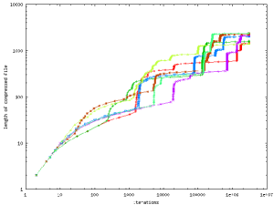
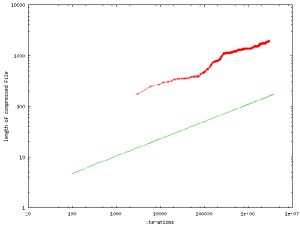
Figure 2: The experimental results for seven different orbits generated by the Manneville map with $z=4$

4.2 The logistic map

We studied the algorithmic complexity also for the logistic map defined by

$$f(x)=\lambda x(1-x)\ ,\quad x\in[0,1]\ ,\quad 1\leq\lambda\leq 4.$$ (8)

The logistic map has been used to simulate the behavior of biological species not in competition with other species. Later the logistic map has also been presented as the first example of a relatively simple map with an extremely rich dynamics. If we let the parameter $\lambda$ vary from $1$ to $4$, we find a sequence of bifurcations of different kinds. For values of $\lambda<\lambda_{\infty}=3.56994567187\dots$, the dynamics is periodic and there is a sequence of period doubling bifurcations which leads to the chaos threshold for $\lambda=\lambda_{\infty}$. The dynamics of the logistic map at the chaos threshold has attracted much attention and many are the applications of theories to the logistic map at this particular value of the parameter $\lambda$. In particular, numerical experiments suggested that at the chaos threshold the logistic map has null K-S entropy, implying that the sensitivity on initial conditions is less than exponential, and there is a power-law sensitivity to initial conditions. These facts have justified the application of generalized entropies to the map ([26],[27]). Moreover, from the relations between initial conditions sensitivity and information content ([16]), we expect to find that the Algorithmic Information Content of the logistic map at the chaos threshold is such that $I_{AIC}(s)\sim\log(n)$ for a $n$-digit long symbolic string $s$ generated by one orbit of the map. We next show how we have experimentally found this result.

From now on $Z$ indicates the compression algorithm CASToRe. It is known that for periodic maps the behavior of the Algorithmic Information Content should be of order $O(\log n)$ for a $n$-long string, and it has been proved that the compression algorithm CASToRe gives for periodic strings $I_{Z}(s)\sim\Pi(n)=\log n\log(\log n)$, where we recall that $I_{Z}(s)$ is the binary length of the compressed string ([8]). In Figure 3, we show the approximation of $I_{Z}(s)$ with $\Pi(n)$ for a $10^{5}$-long periodic string of period 100.

Figure 3: The solid line is the information function for a string $\sigma$ of period 100 compared with $\Pi(N)$ plus a constant term

We have thus used the sequence $\lambda_{n}$ of parameters values where the period doubling bifurcations occur and used a “continuity” argument to obtain the behavior of the information function at the chaos threshold. Another sequence of parameters values $\mu_{k}$ approximating the critic value $\lambda_{\infty}$ from above has been used to confirm the results.

In Figure 4, we plotted the functions $S(n)=\frac{I_{Z}(s)}{\Pi(n)}$ for some values of the two sequences. The starred functions refer to the sequence $\mu_{k}$ and the others to the sequence $\lambda_{n}$. The solid line show the limit function $S_{\infty}(n)$. If we now consider the limit for $n\rightarrow+\infty$, we conjecture that $S_{\infty}(n)$ converges to a constant $S_{\infty}$, whose value is more or less $3.5$. Then we can conclude that, at the chaos threshold, the Algorithmic Information Content of the logistic map is $I_{AIC}(s)\leq I_{Z}(s)\sim S_{\infty}\Pi(n)$. In particular we notice that we obtained an Algorithmic Information Content whose order is smaller than any power law, and we called this behavior mild chaos ([8]).

Figure 4: The solid line is the limit function $S_{\infty}(n)$ and dashed lines are some approximating functions from above (with a star) and below.

5 DNA sequences

We look at genomes as to finite symbolic sequences where the alphabet is the one of nucleotides $\{\mbox{A, C, G, T}\}$ and compute the complexity $K_{Z}$ (where $Z$ is the algorithm CASToRe) of some sequences or part of them.

DNA sequences, in fact, can be roughly divided in different functional regions. First, let us analyze the structure of a Prokaryotic genome: a gene is not directly translated into protein, but is expressed via the production of a messenger RNA. It includes a sequence of nucleotides that corresponds exactly with the sequence of amino acids in the protein (this is the so called colinearity of prokaryotic genes). These parts of the genome are the coding regions. The regions of prokaryotic genome that are not coding are the non coding regions: upstream and downstream regions, if they are proceeding or following the gene.

On the other hand, Eukaryotic DNA sequences have several non coding regions: a gene includes additional sequences that lie within the coding region, interrupting the sequence that represent the protein (this is why these are interrupted genes). The sequences of DNA comprising an interrupted gene are divided into two categories:

• the exons are the sequences represented in the mature RNA and they are the real coding region of the gene, that starts and ends with exons;

• the introns are the intervening sequences which are removed when the first transcription occurs.

So, the non coding regions in Eukaryotic genomes are intron sequences and up/downstream sequences. The last two regions are usually called intergenic regions. In Bacteria and Viruses genomes, coding regions have more extent than in Eukaryotic genomes, where non coding regions prevail.

There is a long-standing interest in understanding the correlation structure between bases in DNA sequences. Statistical heterogeneity has been investigated separately in coding and non coding regions: long-range correlations were proved to exist in intron and even more in intergenic regions, while exons were almost indistinguishable from random sequences ([21],[10]).

Figure 5: On the left, the complexity of coding sequences of Bacterium Escherichia Coli as a function of the length $L$ of the windows are compared to a statistically equivalent random sequence. On the right, the same comparison with respect to the intergenic (non coding) sequence of the same genome.

Figure 6: The analysis of the three functional regions of the genome of Eukaryote Saccharomyces Cerevisiae: the solid line is relative to the coding regions, the dashed line to the intergenic regions, the dotted line to the intron region. The complexities, as functions of length $L$ of the windows, are clearly different from each other. The regions have not similar length so the picture has been drawn according to the shortest region.

Our approach can be applied to look for the non-extensivity of the Information content corresponding to the different regions of the sequences.

We have used a modified version of the algorithm CASToRe, that exploits a window segmentation (see Appendix); let $L$ be the length of a window. We measure the mean complexity of substrings with length $L$ belonging to the sequence that is under analysis. Then, we obtain the Information and the complexity of the sequence as functions of the length $L$ of the windows.

In analogy with physical language, we call a function $f$ extensive if the sum of the evaluations of $f$ on each part of a partition of the domain equals the evaluation of $f$ on the whole domain:

$$\sum_{i\in I}f(A_{i})=f\left(\bigcup_{i\in I}A_{i}\right).$$

In case of a non-extensive function $\tilde{f}$, we have that the average on the different parts underestimates the evaluation on the whole domain:

$$\sum_{i\in I}\tilde{f}(A_{i})\leq\tilde{f}\left(\bigcup_{i\in I}A_{i}\right).$$

Now let us consider the Information Content: each set $A_{i}$ is a window of fixed length $L$ in the genome, so it can be considered as $A_{i}(L)$. Then the related complexity is $\frac{I_{Z}(A_{i}(L))}{L}$.

If a sequence is chaotic or random, then its Information content is extensive, because it has no memory (neither short-range or long range correlations). But if a sequence shows correlations, then the more long-ranged the correlations are the more non-extensive is the related Information content. We have that:

• if the Information content is extensive, the complexity is constant as a linear function of the length $L$;

• if the Information content is non-extensive, the complexity is a decreasing, less than linear function of the length $L$.

From the experimental point of view, we expect our results to show that in coding regions the Information content is extensive, while in non coding regions the extensivity is lost within a certain range $[0,L^{\ast}]$ of window length (the number $L^{\ast}$ depends on the genome). This is also supported by the statistical results exposed above.

In coding sequences, we found that the complexity is almost constant: the compression ratio does not change sensitively with $L$. In non coding sequences, the complexity decreases until some appropriate $L^{\ast}$ is reached and later the compression ratio is almost constant.

This is an information-theoretical proof (alternative to the statistical technique) that coding sequences are more chaotic than non coding ones. Figure 5 shows the complexity of coding (on the left) and non coding (on the right) regions of the genome of Bacterium Escherichia Coli as a function of the length $L$ of the windows and compared with statistically equivalent random sequences. Clearly the compression ratio decreases more in the non coding regions than in the coding ones, where the random sequences show almost constant complexity.

Figure 6 shows the analysis of the three functional regions of the genome of Saccharomyces Cerevisiae which is an eukaryote: the complexities, as functions of length $L$ of the windows, are clearly different from each other. We remark that the lower is the compression ratio, the higher is the aggregation of the words in the genome. This is due to the fact that the algorithm CASToRe recognizes patterns already read, so it is not necessary to introduce new words, but coupling old words to give rise to a new longer one is sufficient to encode the string.

Appendix: CASToRe

The Lempel-Ziv $LZ78$ coding scheme is traditionally used to codify a string according to a so called incremental parsing procedure [20]. The algorithm divides the sequence in words that are all different from each other and whose union is the dictionary. A new word is the longest word in the charstream that is representable as a word already belonging to the dictionary together with one symbol (that is the ending suffix).

We remark that the algorithm $LZ78$ encodes a constant $n$ digits long sequence ${}^{\prime}111\dots^{\prime}$ to a string with length about $const\ +\ n^{\frac{1}{2}}$ bits, while the theoretical Information $I_{AIC}$ is about $const\ +\ \log n$. So, we can not expect that $LZ78$ is able to distinguish a sequence whose Information grows like $n^{\alpha}$ ($\alpha<\frac{1}{2}$) from a constant or periodic one.

This is the main motivation which lead us to create the new algorithm CASToRe. It has been proved in [8] that the Information of a constant sequence, originally with length $n$, is $4+2\log(n+1)[\log(\log(n+1))-1]$, if CASToRe is used. As it has been showed in section 4.1, the new algorithm is also a sensitive device to weak dynamics.

CASToRe is an encoding algorithm based on an adaptive dictionary. Roughly speaking, this means that it translates an input stream of symbols (the file we want to compress) into an output stream of numbers, and that it is possible to reconstruct the input stream knowing the corrispondence between output and input symbols. This unique corrispondence between sequences of symbols (words) and numbers is called the dictionary.

“Adaptive” means that the dictionary depends on the file under compression, in this case the dictionary is created while the symbols are translated.

At the beginning of encoding procedure, the dictionary is empty. In order to explain the principle of encoding, let’s consider a point within the encoding process, when the dictionary already contains some words.

We start analyzing the stream, looking for the longest word W in the dictionary matching the stream. Then we look for the longest word Y in the dictionary where W + Y matches the stream. Suppose that we are compressing an english text, and the stream contains “basketball …”, we may have the words “basket” (number 119) and “ball” (number 12) already in the dictionary, and they would of course match the stream.

The output from this algorithm is a sequence of word-word pairs (W, Y), or better their numbers in the dictionary, in our case (119, 12). The resulting word “basketball” is then added to the dictionary, so each time a pair is output to the codestream, the string from the dictionary corresponding to W is extended with the word Y and the resulting string is added to the dictionary.

A special case occurs if the dictionary doesn’t contain even the starting one-character string (for example, this always happens in the first encoding step). In this case we output a special code word which represents the null symbol, followed by this character and add this character to the dictionary.

Below there is an example of encoding, where the pair (4, 3), is composed from the fourth word ^′AC^′ and the third word ^′G^′.

ACGACACGGAC

word 1: $(0,A)$ –$>$ A

word 2: $(0,C)$ –$>$ C

word 3: $(0,G)$ –$>$ G

word 4: $(1,2)$ –$>$ AC

word 5: $(4,3)$ –$>$ ACG

word 6: $(3,4)$ –$>$ GAC

This algorithm can be used in the study of correlations.

A modified version of the program can be used for study of correlations in the stream: it partition the stream into fixed size segments and proceed to encode them separately. The algorithm takes advantage of replicated parts in the stream. Limiting the encoding to each window separately, could results in longer total encoding. The difference between the length of the whole stream encoded and the sum of the encoding of each window depends on number of correlation between symbols at distance greater than the size of the window. Using different window sizes it is possible to construct a ”spectrum” of correlation.

This has been applied for example on DNA sequences for the study of mid and long-term correlations (see section 5).

Implementation:

The main problem implementing this algorithm is building a structure which allows to efficently search words in the dictionary. To this purpose, the dictionary is stored in a treelike structure where each node is a word X = (W, Y), its parent node being W, and storing a link to the string representing Y. Using this method, in order to find the longest word in the dictionary maching exactly a string, you need only to follow a branching path from the root of the dictionary tree.

References

- [1] Allegrini P., Barbi M., Grigolini P., West B.J., “Dynamical model for DNA sequences”, Phys. Rev. E, 52, 5281-5297 (1995).
- [2] Allegrini P., Grigolini P., West B.J., “A dynamical approach to DNA sequences”, Phys. Lett. A, 211, 217-222 (1996).
- [3] Argenti F., Benci V., Cerrai P., Cordelli A., Galatolo S., Menconi G., “Information and dynamical systems: a concrete measurement on sporadic dynamics”, to appear in Chaos, Solitons and Fractals (2001).
- [4] Batterman R., White H., “Chaos and algorithmic complexity”, Found. Phys. 26, 307-336 (1996).
- [5] Benci V., “Alcune riflessioni su informazione, entropia e complessità”, Modelli matematici nelle scienze biologiche, P.Freguglia ed., QuattroVenti, Urbino (1998).
- [6] Benci V., Bonanno C., Galatolo S., Menconi G., Ponchio F., Work in preparation (2001).
- [7] Bonanno C., “The Manneville map: topological, metric and algorithmic entropy”, work in preparation (2001).
- [8] Bonanno C., Menconi G., “Computational information for the logistic map at the chaos threshold”, arXiv E-print no. nlin.CD/0102034 (2001).
- [9] Brudno A.A., “Entropy and the complexity of the trajectories of a dynamical system”, Trans. Moscow Math. Soc. 2, 127-151 (1983).
- [10] Buiatti M., Acquisti C., Mersi G., Bogani P., Buiatti M., “The biological meaning of DNA correlations”, Mathematics and Biosciences in interaction, Birkhauser ed., in press (2000).
- [11] Buiatti M., Grigolini P., Palatella L., “Nonextensive approach to the entropy of symbolic sequences”, Physica A 268, 214 (1999).
- [12] Chaitin G.J., Information, randomness and incompleteness. Papers on algorithmic information theory., World Scientific, Singapore (1987).
- [13] Galatolo S., “Pointwise information entropy for metric spaces”, Nonlinearity 12, 1289-1298 (1999).
- [14] Galatolo S., “Orbit complexity by computable structures”, Nonlinearity 13, 1531-1546 (2000).
- [15] Galatolo S., “Orbit complexity and data compression”, Discrete and Continuous Dynamical Systems 7, 477-486 (2001).
- [16] Galatolo S., “Orbit complexity, initial data sensitivity and weakly chaotic dynamical systems”, arXiv E-print no. math.DS/0102187 (2001).
- [17] Gaspard P., Wang X.J., “Sporadicity: between periodic and chaotic dynamical behavior”, Proc. Natl. Acad. Sci. USA 85, 4591-4595 (1988).
- [18] Katok A., Hasselblatt B., Introduction to the Modern Theory of Dynamical Systems, Cambridge University Press (1995).
- [19] Lempel A., Ziv A., “A universal algorithm for sequential data compression” IEEE Trans. Information Theory IT 23, 337-343 (1977).
- [20] Lempel A., Ziv J., “Compression of individual sequences via variable-rate coding”, IEEE Transactions on Information Theory IT 24, 530-536 (1978).
- [21] Li W., “The study of DNA correlation structures of DNA sequences: a critical review”, Computers chem. 21, 257-271 (1997).
- [22] Manneville P., “Intermittency, self-similarity and 1/f spectrum in dissipative dynamical systems”, J. Physique 41, 1235-1243 (1980).
- [23] Kosaraju S. Rao, Manzini G., “Compression of low entropy strings with Lempel-Ziv algorithms”, SIAM J. Comput. 29, 893-911 (2000).
- [24] Pesin Y.B., “Characteristic Lyapunov exponents and smooth ergodic theory”, Russ. Math. Surv. 32, PAGINE (1977).
- [25] Toth T.I., Liebovitch L.S., “Models of ion channel kinetics with chaotic subthreshold behaviour” Z. Angew. Math. Mech. 76, Suppl. 5, 523-524 (1996).
- [26] Tsallis C., “Possible generalization of Boltzmann-Gibbs statistics”, J. Stat. Phys. 52, 479 (1988).
- [27] Tsallis C., Plastino A. R., Zheng W.M., “Power-law sensitivity to initial conditions - new entropic representation”, Chaos Solitons Fractals 8, 885-891 (1997).
- [28] Zvorkin A.K., Levin L.A., “The complexity of finite objects and the algorithmic-theoretic foundations of the notion of information and randomness”, Russ. Math. Surv. 25, PAGINE (1970).