Hybrid-Cubic-Rational Semi-Lagrangian Method with the Optimal Mixing

Abstract

A semi-Lagrangian method for advection equation with hybrid cubic-rational interpolation is introduced. In the present method, the spatial profile of physical quantities is interpolated with a combination of a cubic and a rational function. For achieving both high accuracy and convexity preserving of solution, the two functions are mixed in the optimal ratio which is given theoretically. Accuracy and validity of this method is demonstrated with some numerical experiments.

Key Words: Numerical method, Advection, Semi-Lagrangian method, Interpolation, Cubic function, Rational function, Convexity preserving.

I INTRODUCTION

Basically, the CIP method [1, 2] is a numerical method for an advection equation,

$\displaystyle\frac{{\partial f}}{{\partial t}}+u\frac{{\partial f}}{{\partial x}}=0$

whose solution is expressed as

$$f(x,t+\Delta t)=f(X(x,t),t),$$ (1)

where $X$ is the trajectory of fluid particle, which is located at $x$ at the time $t+\Delta t$,

$$X(x,t)=x+\int_{t}^{t-\Delta t}{u(X(x,\tau),\tau)d\tau}.$$ (2)

In a semi-Lagrangian scheme like the CIP, the solution (1) is solved as an interpolation problem [3, 1]. In the CIP scheme, an Hermite cubic expansion function is used to interpolate $f$ at the time $t$. The quantity and its first spatial derivative defined at each grid points are updated as to obey, respectively, eq. (1) and its spatial derivative, i.e.,

$\displaystyle\frac{{\partial f(x,t+\Delta t)}}{{\partial x}}=\frac{{\partial X(x,t)}}{{\partial x}}\frac{{\partial f(X(x,t),t)}}{{\partial X}}$

Generally, the integration in eq. (2) is solved by assuming that $u$ is locally constant as

$$X(x,t) \approx x+u(x,t)\int_{t}^{t-\Delta t}{d\tau}$$ (3)

$$= x-u(x,t)\Delta t.$$ (4)

With this, the solutions (1) and (2) are expressed, respectively, as

$$f(x,t+\Delta t)=f(x-u(x,t)\Delta t,t),$$ (5)

$$\frac{{\partial f(x,t+\Delta t)}}{{\partial x}}=[1-\frac{{\partial u(x,t)}}{{\partial x}}\Delta t]\frac{{\partial f(x-u(x,t)\Delta t,t)}}{{\partial X}}.$$ (6)

In the last decade, various kinds of extension and improvement have been adopted to this method. In 1990, Yabe et al extended this to multidimensions without time-splitting technique by employing a multidimensional cubic expansion function [4]. In 1991, Kondoh extended the 1D CIP to a 5th-order advection method and, furthermore, proposed a solver for parabolic equations by extending the basic concept of the CIP [5]. In the same year, Aoki and Yabe improved the multidimensional one by modifying the multidimensional expansion function and proposed two alternative formulae [6, 7]. In 1994, Kondoh extended his approach to a multidimensional parabolic equation and general hyperbolic equations [8]. In 1995, Ida and Yabe proposed an implicit version of the CIP [9]. This method is CFL free and can be solved directly with a marching procedure although it is a 3rd-order method. In the same year, Utsumi extended the CIP to a solver for the Euler equations of fluid flow without finite-difference technique by employing differential-algebraic and Lagrangian-like concepts [10]. In 1996, Xiao et al proposed a convexity preserving method for the advection equation by replacing the cubic function in the CIP scheme with a cubic-rational function [11, 12]. In the same year, Ida proposed a high accurate solver for free-surface flow problem by coupling the CIP with newly proposed extrapolation scheme [13, 14, 15]. With this method, the density discontinuity at material interface is solved without any numerical dissipation across the interface. In 1997, by extending the Kondoh’s approach [5], Aoki proposed high accurate solver for wave equation, full Euler equations and others [16]. In 1999, Tanaka et al proposed an exactly conservative solver for the continuity equation in non-conservative form by additionally using the local mass of fluid as a dependent variable [17, 18].

In this paper we discuss on the rational method proposed by Xiao et al. As proved theoretically in ref. 11, the rational interpolation method suppresses the numerical oscillation which tends to appear in high-order solution. However, this method sometime provides more diffusive result than that with the classical cubic interpolation. We try to improve its accuracy, without any loss of the convexity preserving property, by mixing with the cubic interpolation function in the optimal ratio. In Sec. 2, the conventional rational method is briefly reviewed and, in Sec. 3, the optimal mixing ratio is given theoretically. In Sec. 4, results of some numerical experiments are shown for demonstrating the accuracy and the validity of the present method.

II CONVEXITY PRESERVING SEMI-LAGRANGIAN METHOD

In the rational method [11], the following cubic-rational interpolation function is used:

$$CR(\xi,\gamma)=\frac{{f_{i}+A1_{i}\xi+A2_{i}\xi^{2}+A3_{i}\xi^{3}}}{{1+\gamma B_{i}\xi}},$$ (7)

where

$$A1_{i} = d_{i}+f_{i}\gamma B_{i},$$ (8)

$$A2_{i} = S_{i}\gamma B_{i}+(S_{i}-d_{i})/h-A3_{i}h,$$ (9)

$$A3_{i} = [d_{i}-S_{i}+(d_{i+1}-S_{i})(1+\gamma B_{i}h)]/h^{2},$$ (10)

$$B_{i} = \left({\frac{{S_{i}-d_{i}}}{{d_{i+1}-S_{i}}}-1}\right)/h,$$ (11)

$$S_{i} = (f_{i+1}-f_{i})/h,$$ (12)

$$\xi = -u_{i}\Delta t,$$ (13)

$f_{i}$ and $d_{i}$ are a physical quantity and its first spatial derivative, respectively, ${u_{i}}$ is the particle velocity at $x_{i}$ assumed as negative here, $\Delta t$ is the time interval, $h$ is the grid width assumed as uniform in this paper for simplicity and $\gamma$ is a parameter for switching the form of the interpolation function. In the case of $\gamma=1$, eq. (7) is reduced to a rational formula of

$$CR(\xi,1)=\frac{{f_{i}+R1_{i}\xi+R2_{i}\xi^{2}}}{{1+B_{i}\xi}},$$ (14)

where

$$R1_{i} = d_{i}+f_{i}B_{i},$$ (15)

$$R2_{i} = S_{i}B_{i}+(S_{i}-d_{i})/h.$$ (16)

Unlike rational functions used in data interpolation technique (See Ref. [19] for example), the above formula is constructed not only with the quantity but also with its derivative. In the case of $\gamma=0$, on the contrary, eq. (7) is reduced to a cubic formula of

$$CR(\xi,0)=f_{i}+C1_{i}\xi+C2_{i}\xi^{2}+C3_{i}\xi^{3},$$ (17)

where

$$C1_{i} = d_{i},$$ (18)

$$C2_{i} = -(2d_{i}+d_{i+1}-3S_{i})/h,$$ (19)

$$C3_{i} = (d_{i}+d_{i+1}-2S_{i})/h^{2}.$$ (20)

Those rational and cubic formulae satisfy a continuity condition at $x_{i}$ and $x_{i+1}$ expressed as

$\displaystyle\left\{{\begin{array}[]{*{20}c}{CR(0,1)=f_{i},\hfill}\\ {CR(h,1)=f_{i+1},\hfill}\\ {\partial_{x}CR(0,1)=d_{i},\hfill}\\ {\partial_{x}CR(h,1)=d_{i+1}.\hfill}\\ \end{array}}\right.$

The rational formula is adapted in a cell where the data is convex or concave, i.e.,

$\displaystyle d_{i}>S_{i}>d_{i+1}$

or

$\displaystyle d_{i}<S_{i}<d_{i+1}.$

This rational interpolation function preserves the convexity of solution. For the other data, interpolation function is switched to the formula of eq. (17) which corresponds to the conventional one of CIP [1] and provides purely 3rd-order solution.

With those interpolation functions, in this paper, we propose a hybrid method of making use only of their superior characteristics by mixing them optimally. In ref. 12, Xiao et al proposed an additional switching technique shown as

$$\gamma=\left\{{\begin{array}[]{*{20}c}{1,\hfill}&{{\rm for}\;d_{i}\cdot d_{i+1}<0,\hfill}\\ {0,\hfill}&{\rm otherwise.\hfill}\\ \end{array}}\right.$$ (21)

This means that the rational function is applied only in the cell which includes a turning point of the gradient. While this procedure modifies the dissipation property of the rational method, this breaks the preserving of convexity as shown in Sec. 4. The optimal mixing technique being proposed in this paper would achieve improvement of accuracy without any loss of the convexity preserving property.

For the convenience of the following discussion, we rearrange eqs. (14) and (17) as

$$R(k)=f_{i}+d_{i}hk+\frac{{P_{i}^{2}k^{2}}}{{Q_{i}+(P_{i}-Q_{i})k}},$$ (22)

and

$$C(k)=f_{i}+d_{i}hk+(2P_{i}-Q_{i})k^{2}+(Q_{i}-P_{i})k^{3},$$ (23)

respectively, where

$$P_{i} = (S_{i}-d_{i})h,$$ (24)

$$Q_{i} = (d_{i+1}-S_{i})h,$$ (25)

and

$\displaystyle k\equiv\xi/h=-u_{i}\Delta t/h$

is the local Courant number and

$\displaystyle k\in[0,1]$

because of the CFL condition.

III HYBRID CUBIC-RATIONAL METHOD WITH THE OPTIMAL MIXING

A The optimal mixing of the two interpolation functions under the convexity-preserving condition

We start from a combination of the rational and the cubic functions shown as

$$F(k)=\alpha R(k)+(1-\alpha)C(k),$$ (26)

where $\alpha$ is a weighting parameter whose range is limited as $\alpha\in[0,1]$. For large $\alpha$, i.e., $\alpha\sim 1$, less oscillatory solution may be expected because the rational function becomes dominant and, for small $\alpha$, i.e., $\alpha\sim 0$, high-order solution may be expected because the cubic one becomes dominant. By determining $\alpha$ properly, convexity-preserving high-accurate method may be produced. We discuss below how to determine the weighting parameter.

While numerous proofs on some characteristics of the rational interpolation method have been done in Ref. [11], the roof of all of them is a property of the rational function. The property is expressed as that, for the convex data, the interpolation function is convex between the given interval and, for the concave data, it is concave. Namely,

$\displaystyle\frac{{\partial^{2}R(k)}}{{\partial x^{2}}}\leq 0,\quad{\rm for}\;k\in[1,0]$

is true for the convex data of

$\displaystyle P_{i}<0\;{\rm and}\;Q_{i}<0,$

and

$\displaystyle\frac{{\partial^{2}R(k)}}{{\partial x^{2}}}\geq 0,\quad{\rm for}\;k\in[1,0]$

is true for the concave data of

$\displaystyle P_{i}>0\;{\rm and}\;Q_{i}>0.$

For achieving both convexity preserving and better resolution, we make the weighting parameter the minimum value which satisfies the above condition. The following discussion will be limited to the case where the data is convex or concave since the rational interpolation is adopted only in the case. For the other data, the cubic interpolation is adopted.

The second spatial derivative of eq. (26) is shown as

$$\frac{\partial^{2}F(k)}{\partial x^{2}} =\alpha\frac{2P_{i}^{2}Q_{i}^{2}}{h^{2}[(P_{i}-Q_{i})k+Q_{i}]^{3}}$$ (28)

$$+(1-\alpha)\frac{2}{h^{2}}[3(Q_{i}-P_{i})k+2P_{i}-Q_{i}].$$

By introducing $H_{i}$ defined as

$\displaystyle H_{i}\equiv\frac{Q_{i}}{P_{i}},$

eq. (28) is rewritten as

$$\frac{{\partial^{2}F(k)}}{{\partial x^{2}}}=\frac{2}{h^{2}}Q_{i}\left\{\alpha\frac{{H_{i}}}{{[(1-H_{i})k+H_{i}]^{3}}}\right.$$ (29)

$$\left.+(1-\alpha)\frac{{3(H_{i}-1)k+2-H_{i}}}{{H_{i}}}\right\}.$$ (30)

For preserving convexity of solution, as mentioned above, the following condition must be satisfied:

$\displaystyle\frac{{\partial^{2}F(k)}}{{\partial x^{2}}}\leq 0,\quad{\rm for}\;P_{i}<0\;{\rm and}\;Q_{i}<0,$

or

$\displaystyle\frac{{\partial^{2}F(k)}}{{\partial x^{2}}}\geq 0,\quad{\rm for}\;P_{i}>0\;{\rm and}\;Q_{i}>0.$

This condition is expressed by an inequality of

$${{\frac{{\partial^{2}F(k)}}{{\partial x^{2}}}}\mathord{\left/{\vphantom{{\frac{\partial^{2}F(k)}{\partial x^{2}}}{\left({\frac{{h^{2}}}{2}Q_{i}}\right)}}}\right.\kern-1.2pt}{\left({\frac{2}{h^{2}}Q_{i}}\right)}}=\alpha\frac{H_{i}}{[(1-H_{i})k+H_{i}]^{3}}$$ (31)

$$+(1-\alpha)\frac{{3(H_{i}-1)k+2-H_{i}}}{{H_{i}}}\geq 0,$$ (32)

because the sigh of ${{\partial^{2}F(k)}\mathord{\left/{\vphantom{{\partial^{2}F(k)}{\partial x^{2}}}}\right.\kern-1.2pt}{\partial x^{2}}}$ and $Q_{i}$ should be the same. Furthermore, the inequality (31) can be rewritten as

$$\alpha H_{i}^{2}+(1-\alpha)G_{i}^{3}[3(H_{i}-1)k+2-H_{i}]\geq 0,$$ (33)

where

$\displaystyle G_{i}\equiv(1-H_{i})k+H_{i},$

because of

$$H_{i}>0$$ (34)

(Remind that the signs of $P_{i}$ and $Q_{i}$ are the same) and

$$G_{i}\geq{\rm min}(1,H_{i})>0,\quad{\rm for}\;k\in[0,1].$$ (35)

Here we introduce $K_{i}(k)$ which is defined as

$\displaystyle K_{i}(k)\equiv G_{i}^{3}[3(H_{i}-1)k+2-H_{i}].$

With this function, eq. (33) is rewritten as

$$\alpha H_{i}^{2}+(1-\alpha)K_{i}(k)\geq 0.$$ (36)

From the inequality (35) and

$$3(H_{i}-1)k+2-H_{i} \geq {\rm min}(2-H_{i},2H_{i}-1),$$ (37)

$${\rm for}\;k \in [0,1],$$ (38)

it is known that the inequality (36) is always true for

$\displaystyle 1/2\leq H_{i}\leq 2$

because of $K_{i}(k)\geq 0$. In this case, we can use $\alpha=0$, i.e., the purely cubic interpolation function which provides high-order solution.

For a while, the following discussion will be limited to the case of

$\displaystyle H_{i}>2.$

The first and the second spatial derivatives of $K_{i}(k)$ respect to $k$ are

$$\frac{{\partial K_{i}(k)}}{{\partial k}}=6(1-H_{i})^{2}G_{i}^{2}(1-k)$$ (39)

and

$$\frac{{\partial^{2}K_{i}(k)}}{{\partial k^{2}}}=6(1-H_{i})^{2}G_{i}(2-3G_{i}),$$ (40)

respectively. From eq. (40) with an inequality of

$\displaystyle G_{i}\geq\min(1,H_{i})=1,\quad{\rm for}\;H_{i}\geq 2\;{\rm and}\;k\in[0,1],$

we know that

$\displaystyle\frac{\partial^{2}K_{i}(k)}{\partial k^{2}}<0,\quad{\rm for}\;k\in[0,1],$

which means that ${{\partial K_{i}(k)}\mathord{\left/{\vphantom{{\partial K_{i}(k)}{\partial k}}}\right.\kern-1.2pt}{\partial k}}$ is monotonicaly decreasing for $k\in[0,1]$. Furthermore, from eq. (39), we know that

$\displaystyle\frac{{\partial K_{i}(0)}}{{\partial k}}=6(1-H_{i})^{2}H_{i}^{2}>0$

and

$\displaystyle\frac{{\partial K_{i}(1)}}{{\partial k}}=0.$

Namely, ${{\partial K_{i}(k)}\mathord{\left/{\vphantom{{\partial K_{i}(k)}{\partial k}}}\right.\kern-1.2pt}{\partial k}}$ has non-negative value for $k\in[0,1]$.

Those results show that $K_{i}(k)$ is monotonicaly increasing for $k\in[0,1]$, and the minimum value of it is

$\displaystyle{\rm min}(K_{i}(k))=K_{i}(0)=H_{i}^{3}(2-H_{i})<0.$

Thus, the inequality (36) is reduced to

$\displaystyle\alpha H_{i}^{2}+(1-\alpha)H_{i}^{3}(2-H_{i})\geq 0.$

From this, we get

$\displaystyle\alpha\geq\frac{{H_{i}(H_{i}-2)}}{{H_{i}(H_{i}-2)+1}}.$

For increasing the dominance of the cubic function as much as possible, we use

$$\alpha=\frac{{H_{i}(H_{i}-2)}}{{H_{i}(H_{i}-2)+1}}.$$ (41)

The proof for the case of

$\displaystyle 0<H_{i}<1/2$

can be done easily as follows. With replacements of

$$\left\{{{\begin{array}[]{*{20}c}{H_{i}\to 1/L_{i},\hfill}\\ {k\to l-1,\hfill}\\ \end{array}}}\right.$$ (42)

the inequality (33) is rewritten as

$\displaystyle\alpha L_{i}^{2}+(1-\alpha)[(1-L_{i})l+L_{i}]^{3}[3(L_{i}-1)l+2-L_{i}]\geq 0.$

This inequality corresponds to that of (33) only with replacements of $L_{i}\to H_{i}$ and $l\to k$. Thus, the solution of this inequality is

$$\alpha\geq\frac{{L_{i}(L_{i}-2)}}{{L_{i}(L_{i}-2)+1}},\quad{\rm for}\;L_{i}>2\;{\rm and}\;l\in[0,1].$$ (43)

From eq. (42), it is known that the result (43) is for $0<H_{i}\;<1/2$ and $k\in[0,1]$. From the same reason as mentioned in leading eq. (41), we use

$$\alpha=\frac{{L_{i}(L_{i}-2)}}{{L_{i}(L_{i}-2)+1}}.$$ (44)

The above results on the determination of $\alpha$ is summarized as

$$\alpha=\frac{{M_{i}(M_{i}-2)}}{{M_{i}(M_{i}-2)+1}},$$ (45)

where

$$M_{i} = \max[2,\;\max(H_{i},\;L_{i})]$$ (46)

$$= \max[2,\;\max(\frac{{Q_{i}}}{{P_{i}}},\;\frac{{P_{i}}}{{Q_{i}}})].$$ (47)

In the case of $1/2\leq H_{i}\leq 2$ and $H_{i}\leq 0$, $M_{i}$ and $\alpha$ are determined with eqs. (46) and (45) as

$$M_{i}=2,$$ (48)

$$\alpha=0,$$ (49)

and the interpolation function is reduced to pure cubic. For $H_{i}\geq 2$, eq. (45) is reduced to eq. (41) and, for $L_{i}\geq 2$, it is reduced to eq. (44).

B Summary of the formula

With a little rearrangement, the formula derived in the last subsection is summarized as

$\displaystyle F(k)=f_{i}+d_{i}hk+(G1_{i}+G2_{i})k^{2},$

$\displaystyle\frac{{\partial F(k)}}{{\partial x}}=d_{i}+[G1_{i}\frac{{Q_{i}+D_{i}}}{{D_{i}}}+2G2_{i}+(1-\alpha)(Q_{i}-D_{i})]\frac{{k}}{{h}},$

where

$$G1_{i} = \alpha P_{i}^{2}/D_{i},$$ (50)

$$G2_{i} = (1-\alpha)(2P_{i}-D_{i}),$$ (51)

$$D_{i} = Q_{i}+(P_{i}-Q_{i})k,$$ (52)

$$\alpha = \frac{{M_{i}(M_{i}-2)}}{{M_{i}(M_{i}-2)+1}},$$ (53)

$$M_{i} = max[2,\;max(\frac{{Q_{i}}}{{P_{i}}},\;\frac{{P_{i}}}{{Q_{i}}})]$$ (54)

with

$$P_{i} = (S_{i}-d_{i})h,$$ (55)

$$Q_{i} = (d_{i+1}-S_{i})h,$$ (56)

$$S_{i} = (f_{i+1}-f_{i})/h.$$ (57)

For the case of $u_{i}>0$, we need replacements of

$\displaystyle i+1\to i-1,\quad h\to-h.$

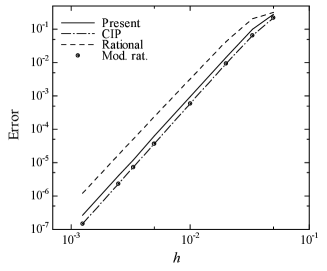
FIG. 1.: Numerical error as a function of the grid width $h$ in the results with the present, the CIP, the conventional rational and the modified rational (with the additional switching technique) methods.

IV NUMERICAL EXPERIMENTS

For demonstrating the validity of the previous discussions and the accuracy of the present scheme, we show some numerical experiments in this section.

The first example is the linear propagation of a sinusoidal wave. The initial condition is

$\displaystyle f(i,0)=0.5\cos(4\pi h\,i),$

where the grid width $h$ is set in this example as

$\displaystyle h=1/N$

and $N$ is the number of grid points. The velocity is set as $u=1$ and is assumed as constant in space and time. The boundary condition at $i=0$ and $N$ is periodic. With this example, we compare the accuracy of the present method with that of the three existing methods, i.e., the CIP, the conventional rational method and that with the additional switching (21). The last one is called below the modified rational method. Here we define numerical error as

$\displaystyle{\rm Error}=\frac{{\sum\limits_{i=1}^{N}{\left|{f_{i}^{n}-{\rm analytical\;value}}\right|}}}{{N}},$

where the superscript $n$ shows the number of time step. In Fig. 1, we plot the error as a function of the grid width $h$ at $n=4000$ with CFL = 0.2. From this result, it is known that the accuracy of the methods except for the conventional rational method are very similar each other on this problem, while that of the present one is inferior a few among them.

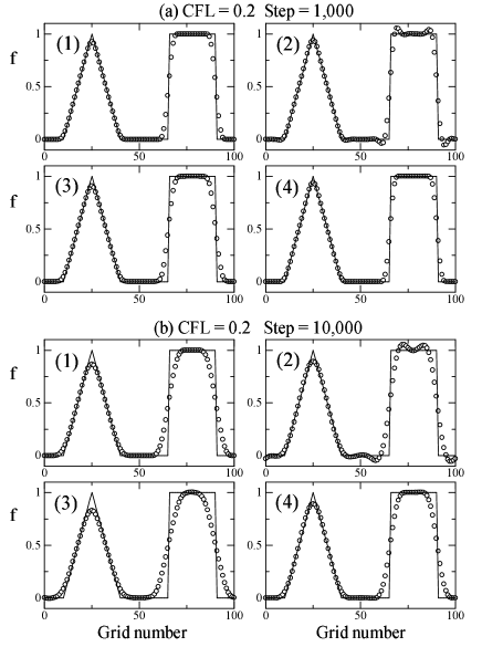
FIG. 2.: Linear propagation of a triangular and a square waves. The figure shows results at $n=1,000$ (the upper group) and $n=10,000$ (the lower group) with the present (1), the CIP (2), the conventional rational (3) and the modified rational (4) methods.

Next we solve the linear propagation of a triangular and a square wave. The pulse widths of the waves are $30h$ and $26h$, respectively, and pulse heights are 1. In Fig. 2, we show results at $n=1,000$ (a) and 10,000 (b) with CFL = 0.2. In the results with the CIP method, overshoots and undershoots are obviously shown around the discontinuities of the square wave. The results with the conventional rational method are more diffusive than other ones. The results with the present and the modified rational method are very similar while the former one is more diffusive quite a little and the latter one has small over- and undershoots.

With the same example of the square wave, we further discuss on the convexity preserving property of those methods. Here we introduce a variable $p$ defined as

$\displaystyle p_{i+1/2}^{n}=\left\{{{\begin{array}[]{*{20}c}{1/2,}&{{\rm if}\;f_{i+1}^{n}-f_{i}^{n}>0,}\\ {0,}&{{\rm if}\;f_{i+1}^{n}-f_{i}^{n}=0,}\\ {-1/2,}&{{\rm if}\;f_{i+1}^{n}-f_{i}^{n}<0.}\\ \end{array}}}\right.$

By observing this variable, we can appreciate the convexity of solution. In Fig. 3, we show $f$ and $p$ at $n=150$ (a) and $10,000$ (b). Analytically, $p$ becomes $1/2$ and $-1/2$ only at the left and right discontinuities, respectively, and $p=0$ elsewhere, namely, only one positive and one negative regions should exist in the spatial profile of $p$ if the convexity of $f$ is preserved. In the results with the present and the conventional rational method, the two regions are clearly seen while the width of the regions is expanded by the numerical diffusion. In the results with the CIP and the modified rational methods, many numbers of leaps are shown in the profile of $p$. This means that the conventional CIP and the modified rational methods are not oscillation free.

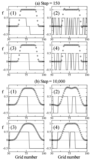
FIG. 3.: Results of the linear propagation of a square wave at $n=150$ (the upper group) and $n=10,000$ (the lower group) with the present (1), the CIP (2), the conventional rational (3) and the modified rational (4) methods. The circles and the solid lines show $f$ and $p$, respectively.

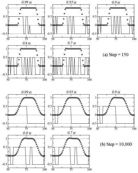
FIG. 4.: Results with the reduced mixing ratio (0.99, 0.95, 0.9, 0.8 and 0.7 times values of the optimal one) at $n=150$ (the upper group) and $n=10,000$ (the lower group).

In order to demonstrate that the determination of $\alpha$ with eq. (45) is the optimal, we show results of the same example with the present method and reduced $\alpha$. In Fig. 4, we show results with 0.99, 0.95, 0.9, 0.8 and 0.7 times smaller value of $\alpha$ than that is determined with eq. (45) and CFL = 0.2. The unphysical oscillation is observed even in the results with 0.99 times value and the oscillation becomes stronger according as $\alpha$ decreases. The numerical oscillation at $n=10,000$ becomes weaker than that at $n=150$ because of numerical diffusion, but still exists. The overshoot around the discontinuity of $f$ can also be seen in those results and it becomes larger as $\alpha$ decreases.

Finally we show results of an extreme example for demonstrating the robustness of the present method and a defect of the modified rational method. The initial profiles of $f$ and $u$, the latter is assumed as constant in time, for this example are shown in Fig. 5. In the initial profile of $f$, there exist two steep gradients which are appropriately smooth but sufficiently sharp. In the velocity distribution, a similar gradient exists, and $u=1$ in the left side of the gradient and $u=0.1$ in the right side. Those mollified profiles are made as follows: First $f$ and $u$ are set as

$\displaystyle f_{i}=\left\{{\begin{array}[]{*{20}c}{1,\hfill}&{{\rm for}\;5\leq i\leq 67,\hfill}\\ {0,\hfill}&{{\rm elsewhere\hfill}}\\ \end{array}}\right.$

and

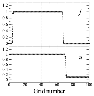
FIG. 5.: Initial condition of the extreme example. The upper and the lower figures show $f$ and $u$, respectively.

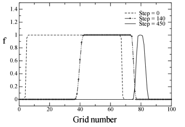
FIG. 6.: A typical result of the extreme example by using the present method. The figure shows results at $n=0$, 140 and 450 with CFL = 0.25.

$\displaystyle u_{i}=\left\{{\begin{array}[]{*{20}c}{1,\hfill}&{{\rm for}\;i\leq 71,\hfill}\\ {0.1,\hfill}&{\rm elsewhere.\hfill}\\ \end{array}}\right.$

Next, those values are smoothed with a conventional 3-point smoother,

$$g_{i}^{(m+1)} = (1-\varepsilon)g_{i}^{(m)}+\varepsilon\frac{{g_{i+1}^{(m)}+g_{i-1}^{(m)}}}{{2}},$$ (58)

$${\rm for} \;m=1,2,\cdots M,$$ (59)

where $g$ is $f$ or $u$, $m$ is the iteration number of the smoothing, $M$ is the maximum of it and $\varepsilon$ is a positive constant smaller than 1.0. For $f$ and $u$, we use $(M,\varepsilon)=(2,0.05)$ and $(2,0.1)$, respectively. The resulting mollified values are used as initial values. Initial value of $d_{i}$ is set as

$\displaystyle d_{i}^{0}=\left\{{\begin{array}[]{*{20}c}{0,\hfill}&{{\rm if}\;f_{i}^{(M)}=0\;{\rm or}\;f_{i}^{(M)}=1,\hfill}\\ {(f_{i+1}^{(M)}-f_{i-1}^{(M)})/2h,\hfill}&{{\rm elsewhere.\hfill}}\\ \end{array}}\right.$

In solving this example, we estimate the velocity gradient appearing in eq. (6) with a conventional second-order centered finite differencing as usually done in the CIP scheme [1].

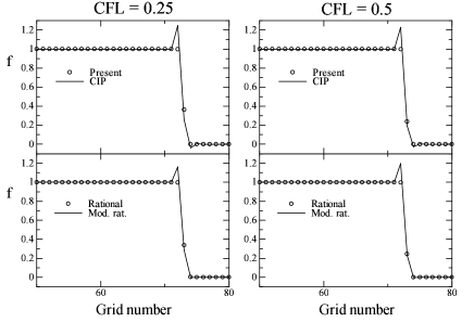
FIG. 7.: Results when the right discontinuity just passes through the velocity gradient (the left group:$n=48$ with CFL = 0.25. the right group: $n=24$ with CFL = 0.5). In the results with the CIP and the modified rational methods, strong overshoot appears.

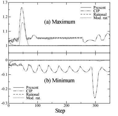
FIG. 8.: The maximum (upper) and the minimum (lower) values in the numerical results of the extreme example as a function of the time step. The maximum and the minimum values calculated with the present and the conventional rational methods keep with 1 and 0, respectively, while those with the CIP and the modified rational method are oscillated.

In the first stage of this problem, the mollified square wave of $f$ propagates to right in $u=1$. Then, after the wave covers the gradient of $u$, the waveform is compressed in horizontal direction and the pulse width is decreased. Finally, after passing through the velocity gradient, the width of the square becomes 1/10 of the initial one, i.e., $\sim 6h$, and the square propagates in $u=0.1$ (See Fig. 6 in which a typical result of this problem by the present method is shown).

In Fig. 7, we show results at $n=48$ with CFL = 0.25 and at $n=24$ with CFL = 0.5. While the results with the present and the conventional rational methods are smooth and oscillation free, strong overshoot is shown in those with the CIP and the modified rational methods. At the time where the gradient of $f$ passes through the gradient of $u$, it is amplified strongly by the velocity gradient. Thus, if the cubic interpolation is adopted in this case, the overshoot should appear. In Fig. 8, we show the maximum and the minimum value of $f$ as a function of the number of time step. The maximums with the CIP and the modified rational methods have strong peak at $n\sim 50$, i.e., when the right gradient of $f$ passes through the velocity gradient and, furthermore, the minimum with the CIP has strong peak at $n\sim 300$, i.e., when the left gradient of $f$ passes through there. This result shows that the additional switching (21) raises inadequate adaptation of the cubic function. The present method does not have such a defect. In Fig. 9, the results at $n=550$, i.e., those after the pulse has passed through the velocity gradient is shown. The result with the modified rational method has weak overshoot and that with the conventional rational method is more diffusive than that with the present one.

The above results prove that the present method has higher accuracy than that of the conventional rational method and is a convexity-preserving method.

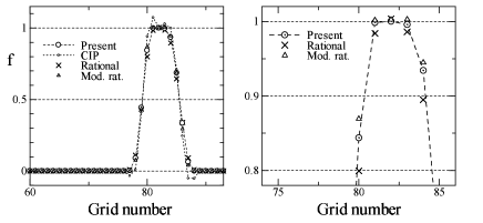
FIG. 9.: Results after the square have passed through the velocity gradient ($n=550$ with CFL = 0.25). The right figure shows an enlarged one of a part of the left one. The result with the CIP is not shown in the right figure. Theoretically the height and the width of the projection should be 1 and about $6h$, respectively.

V CONCLUSION

In this paper we proposed a hybrid semi-Lagrangian method with a cubic and a rational interpolation functions. The optimal ratio for mixing those functions was led theoretically. The present method has higher accuracy than the conventional rational method and is oscillation free. The numerical experiments curried out in the last section demonstrate the validity of the theoretical discussion in Sec. 3 and the accuracy of the present method. However, the results show a limit of the present method as well. Higher accuracy than that of the given results shown, for example, in Figs. 2 and 3 may no longer be expected when one use the cubic and the rational functions under the convexity preserving condition. Extension to a higher-order method may be needed for achieving higher resolution.

The present method may be extended to multidimensions and a conservative method by employing the approaches discussed by Aoki [6, 7] and Tanaka et al [17, 18], respectively.

REFERENCES

• [1] T. Yabe and T. Aoki, A universal solver for hyperbolic equations by cubic-polynomial interpolation I. One-dimensional solver, Comput. Phys. Commun. 60 (1991) pp.219-232.
• [2] T. Yabe, T. Ishikawa, P. Y. Wang, T. Aoki, Y. Kadota and F. Ikeda, A universal solver for hyperbolic equations by cubic-polynomial interpolation II. Two- and three-dimensional solvers, Comput. Phys. Commun. 66 (1991) pp.233-242.
• [3] D. R. Durran, Numerical methods for wave equations in geophysical fluid dynamics, Springer, Sec. 6, p.303.
• [4] T. Yabe, T. Ishikawa and Y. Kadota, A multidimensional cubic-interpolated pseudoparticle (CIP) method without time splitting technique for hyperbolic equations, F. Ikeda, J. Phys. Soc. Japan 59 (1990) pp.2301-2304.
• [5] Y. Kondoh, On thought analysis of numerical scheme for simulation using kernel optimum nearly-analytical discretization (KOND) method, J. Phys. Soc. Japan. 60 (1991) pp.2851-2861.
• [6] T. Aoki and T. Yabe, Multidimensional cubic interpolation for ICF hydrodynamics simulation, NIFS-82, 1991, pp.1-9 (unpublished).
• [7] T. Aoki, Multi-dimensional advection of CIP (Cubic-Interpolated Propagation) scheme, CFD J. 4 (1995) pp.279-292.
• [8] Y. Kondoh, Y. Hosaka and K. Ishii, Kernel optimum nearly-analytical discretization (KOND) algorithm applied to parabolic and hyperbolic equations, Comput. Math. Appl. 27 (1994) pp.59-90.
• [9] M. Ida and T. Yabe, Implicit CIP (cubic interpolated propagation) method in one dimension, Comput. Phys. Commun. 92 (1995) pp.21-26.
• [10] T. Utsumi, Differential algebraic hydrodynamics solver with cubic-polynomial interpolation, CFD J. 4 (1995) pp.225-238.
• [11] F. Xiao, T. Yabe and T. Ito, Constructing oscillation preventing scheme for advection equation by rational function, Comput. Phys. Commun. 93 (1996) pp.1-12.
• [12] F. Xiao, T. Yabe, G. Nizam and T. Ito, Constructing multi-dimensional oscillation preventing scheme for advection equation by rational function, Comput. Phys. Commun. 94 (1996) pp.103-118.
• [13] M. Ida, An improved unified solver for compressible and incompressible fluids involving free surfaces. Part I. Convection, Comput. Phys. Commun. 132 (2000) pp.44-65.
• [14] M. Ida, “Non-smooth solution of density jump at interfaces with discontinuous interpolation and a level set approach”, in: Proc. 10th Symp. on Comput. Fluid. Dynam., Tokyo, Japan, 1996, pp.382-383 (in Japanese. Most all of this content is included in Ref. [13]).
• [15] M. Ida, “Free-surface flow simulation by an interpolation-extrapolation hybrid scheme”, in: Proc. 10th Comput. Mech. Conf., Tokyo, Japan, 1997, pp.17-18 (in Japanese. Most all of this content is included in Ref. [13]).
• [16] T. Aoki, Comput. Phys. Commun. Interpolated differential operator (IDO) scheme for solving partial differential equations, 102 (1997) pp.132-146.
• [17] R. Tanaka, T. Nakamura and T. Yabe, Constructing exactly conservative scheme in anon-conservative form, Comput. Phys. Commun. 126 (2000) pp.232-243.
• [18] R. Tanaka, T. Nakamura and T. Yabe, “Constructing exactly conservative scheme in non-conservative form”, in: Proc. 13th Symp. on Comput. Fluid. Dynam., Tokyo, Japan, 1999, pp.1-5 (in Japanese. unpublished).
• [19] J. C. Clements, Convexity-preserving piecewise rational cubic interpolation, SIAM J. Numer. Anal. 27 (1990) pp.1016-1023.