The honeycomb model of ${{GL_{n}({\mathbb{C}})}}$ tensor products II:
Puzzles determine facets of the Littlewood-Richardson cone

Abstract.

The set of possible spectra $(\lambda,\mu,\nu)$ of zero-sum triples of Hermitian matrices forms a polyhedral cone [H], whose facets have been already studied in [Kl, HR, T, Be] in terms of Schubert calculus on Grassmannians. We give a complete determination of these facets; there is one for each triple of Grassmannian Schubert cycles intersecting in a unique point. In particular, the list of inequalities determined in [Be] to be sufficient is in fact minimal.

We introduce puzzles, which are new combinatorial gadgets to compute Grassmannian Schubert calculus, and seem to have much interest in their own right. As the proofs herein indicate, the Hermitian sum problem is very naturally studied using puzzles directly, and their connection to Schubert calculus is quite incidental to our approach. In particular, we get new, puzzle-theoretic, proofs of the results in [H, Kl, HR, T, Be].

Along the way we give a characterization of “rigid” puzzles, which we use to prove a conjecture of W. Fulton: “if for a triple of dominant weights $\lambda,\mu,\nu$ of ${{GL_{n}({\mathbb{C}})}}$ the irreducible representation $V_{\nu}$ appears exactly once in $V_{\lambda}{\otimes}V_{\mu}$, then for all $N\in{\mathbb{N}}$, $V_{N\lambda}$ appears exactly once in $V_{N\lambda}{\otimes}V_{N\mu}$.”

1. Introduction, and summary of results

We continue from [Hon1] the study of the cone ${\tt BDRY}(n)$, which is the set of triples of weakly decreasing $n$-tuples $(\lambda,\mu,\nu)\in({\mathbb{R}}^{n})^{3}$ satisfying three conditions proved there to be equivalent:

1. regarding $\lambda,\mu,\nu$ as spectra of $n\times n$ Hermitian matrices, there exist three Hermitian matrices with those spectra whose sum is the zero matrix;

2. (if $\lambda,\mu,\nu$ are integral) regarding $\lambda,\mu,\nu$ as dominant weights of ${{GL_{n}({\mathbb{C}})}}$, the tensor product $V_{\lambda}{\otimes}V_{\mu}{\otimes}V_{\nu}$ of the corresponding irreducible representations has an invariant vector;

3. regarding $\lambda,\mu,\nu$ as possible boundary data on a honeycomb, there exist ways to complete it to a honeycomb.

In the present paper we determine the minimal set of inequalities defining this cone, along the way giving new proofs of the results in [HR, T, Kl, Be] which gave a sufficient list of inequalities in terms of Schubert calculus on Grassmannians. We show that this list is in fact minimal (establishing the converse of the result in [Be]). As in [Hon1], our approach to this cone is in the honeycomb formulation. We also replace the use of Schubert calculus by puzzles, defined below.

1.1. Prior work.

Most prior work was stated in terms of the sum-of-Hermitian matrices problem. That was first proved to give a polyhedral cone in [H]. Many necessary inequalities were found (see [F1] for a survey), culminating in the list of Totaro [T], Helmke-Rosenthal [HR], and Klyachko [Kl] – hereafter we call this the H-R/T/K result. Klyachko proved also that this list is sufficient. A recursively defined list of inequalities had been already conjectured in [H]; this conjecture is true, and in fact gives the same list as Klyachko’s – see [Hon1].

One of us (CW) observed that this list is redundant – some of the inequalities given do not determine facets but only lower-dimensional faces of ${\tt BDRY}(n)$ – and proposed a criterion for shortening the list (again in terms of Schubert calculus). That this shorter list is already sufficient was proved by Belkale [Be]. Our primary impetus for the present work was to prove the converse: each of these inequalities is essential, i.e. determines a facet of ${\tt BDRY}(n)$.

1.2. Puzzles.

A puzzle will be a certain kind of diagram in the triangular lattice in the plane. There are three puzzle pieces:

1. unit equilateral triangles with all edges labeled $0$

2. unit equilateral triangles with all edges labeled $1$

3. unit rhombi (two equilateral triangles joined together) with the outer edges labeled $1$ if clockwise of an obtuse angle, $0$ if clockwise of an acute angle.

A puzzle of size $n\in{\mathbb{N}}$ is a decomposition of a lattice triangle of side-length $n$ into lattice polygons, all edges labeled $0$ or $1$, such that each region is a puzzle piece. Some examples are in figure 1.

Figure 1. Some examples of puzzles.

The main result about these puzzles (theorem 1, stated below, proved in section 5) is that they compute Schubert calculus on Grassmannians. While there are many other rules for such computations, e.g. the Littlewood-Richardson rule, this one has the greatest number of manifest symmetries. (A lengthy discussion of this will appear in [KT2].)

Readers only interested in a solution to the Hermitian sum problem can skip the statement of this theorem and, in fact, quit after section 4. A central principle in the current paper is that in determining the facets of ${\tt BDRY}(n)$, the connection to Schubert calculus is quite irrelevant, and it is more natural combinatorially to work with the puzzles directly, which we do until section 5. This nicely complements the principle of [Hon1], in which we worked not with triples of Hermitian matrices but used honeycombs as their combinatorial replacement. We will not in general take space to repeat the honeycomb-related definitions from [Hon1].

We fix first our conventions to describe “Schubert calculus,” which in modern terms is the ring structure on the cohomology of Grassmannians. To an $n$-tuple $\sigma$ like $00101\ldots 110$ of $r$ ones and $n-r$ zeroes, let ${\mathbb{C}}^{\sigma}$ denote the corresponding coordinate $r$-plane in ${\mathbb{C}}^{n}$, and $X_{\sigma}$ the Schubert cycle defined as

$$\big{\{}V_{r}\in{\rm Gr}_{r}({\mathbb{C}}^{n})\quad:\quad\dim(V_{r}\cap F_{i})\geq\dim({\mathbb{C}}^{\sigma}\cap F_{i}),\quad\forall i\in[1,n]\big{\}}$$

where $\{F_{i}\}$ is the standard flag in ${\mathbb{C}}^{n}$. Alternately, $X_{\sigma}$ is the closure of the set of $r$-subspaces $V_{r}\leq{\mathbb{C}}^{n}$ such that $\sigma_{i}=\dim((V_{r}\cap F_{i})/(V_{r}\cap F_{i-1})),i\in[1,n]$. The Schubert class $S_{\sigma}\in H^{*}({\rm Gr}_{r}({\mathbb{C}}^{n}))$ is the Poincaré dual of this cycle. These are well-known to give a basis for the cohomology ring.

Theorem 1.

Let $\pi,\rho,\sigma$ be three $n$-tuples of $r$ ones and $n-r$ zeroes, indexing Schubert classes $S_{\pi},S_{\rho},S_{\sigma}$ in $H^{*}({\rm Gr}_{r}({\mathbb{C}}^{n}))$. Then the following (equivalent) statements hold:

1. The intersection number $\int_{{\rm Gr}_{r}({\mathbb{C}}^{n})}S_{\pi}S_{\rho}S_{\sigma}$ is equal to the number of puzzles whose NW boundary edges are labeled $\pi$, NE are labeled $\rho$, and S are labeled $\sigma$, all read clockwise.

2. $$S_{\pi}\,S_{\rho}=\sum_{\hbox{puzzles $P$ }}S_{\hbox{southern side of $P$, read left to right}}$$

   where the sum is taken over puzzles with NW side labeled $\pi$, NE side labeled $\rho$, both from left to right.

This first is the advertised $Z_{3}$-invariant formulation. The second formulation is very suitable for computations; an example is in figure 2.

Figure 2. The four puzzles $P$ with NW and NE boundaries each labeled $010101$, computing $S_{010101}^{2}=S_{110001}+2S_{101010}+S_{011100}$ in $H^{*}({\rm Gr}_{3}({\mathbb{C}}^{6}))$.

Puzzles have another symmetry, which we call puzzle duality: the dualization of a puzzle is defined to be the left-right mirror reflection, with all $0$s exchanged for $1$s and vice versa. This realizes combinatorially another symmetry of Schubert calculus, coming from the isomorphism of the $r$-Grassmannian in an $n$-dimensional space $V$ with the $(n-r)$-Grassmannian in $V^{*}$. We will use puzzle duality to reduce the number of cases considered in some arguments.

1.3. Organization of this paper.

In sections 2-4 we classify the facets of ${\tt BDRY}(n)$ in terms of puzzles. In sections 5-6 we prove and make use of the connection of puzzles to Schubert calculus. To emphasize again: the reader who is only looking for the minimal list of inequalities determining ${\tt BDRY}(n)$ may completely ignore this connection, and take puzzles as the more relevant concept than Schubert calculus!

Here is a slightly more detailed breakdown of the paper. In section 2 we prove the puzzle-theoretic analogue of the H-R/T/K result: each puzzle gives an inequality on ${\tt BDRY}(n)$.

In section 3 we essentially repeat Horn’s analysis of the facets of ${\tt BDRY}(n)$, but in the honeycomb framework; the analogues of his direct sums turn out to be clockwise overlays. Using these we prove the puzzle-theoretic analogue of Klyachko’s sufficiency result (a converse of H-R/T/K): every facet comes from a puzzle. Easy properties of puzzles (from section 5) then imply Horn’s results (but not his conjecture).

In section 4 we study “gentle loops” in puzzles, and show that the minimal list of inequalities is given by puzzles with no gentle loops. Then comes the only particularly technical part of the paper: showing that puzzles without gentle loops are exactly the rigid ones, meaning those determined by their boundary conditions. That the rigid-puzzle inequalities are a sufficient list is the puzzle analogue of Belkale’s result [Be]; conversely, that every rigid-puzzle inequality determines a facet, is the central new result of this paper.

In section 5 we describe the connection of puzzles to Schubert calculus, and in section 6 give puzzle-free statements of our theorems. This section also serves as a summary of the old and new results in this paper.

Since Schubert calculus is itself related to the tensor product problem (in a lower dimension), this gives a combinatorial way to understand the still-mysterious Horn recursion. We also give an application of the no-gentle-loop characterization of rigid puzzles to prove an unpublished conjecture of W. Fulton.

In the last section we state the corresponding results for sums of $m$ Hermitian matrices. The proofs extend almost without change to the $m\geq 3$ case. In an appendix we give a quick proof of the equivalence between the three definitions of ${\tt BDRY}(n)$, replacing Klyachko’s argument by the Kirwan/Kempf-Ness theorem, which allows for rather stronger results.

Since completing this work, we received the preprint [DW1], which studies representations of general quivers; our results can be seen as concerning the very special case of the “triple flag quiver”. Assuming Fulton’s conjecture as input (see conjecture 30 of [DW1]), their results provide a (completely different) proof of the converse of Belkale’s result. We have been unable to find any generalization of our honeycomb and puzzle machinery to general quivers.

We are most grateful to Anda Degeratu for suggesting the name “puzzle”, and the referee for many useful comments. The once-itinerant first author would like to thank Rutgers, UCLA, MSRI, and especially Dave Ben-Zvi for their gracious hospitality while part of this work was being done.

2. Puzzles give inequalities on ${\tt BDRY}(n)$

In this section we determine a list of inequalities satisfied by ${\tt BDRY}(n)$, which will eventually be seen to be the puzzle-theoretic version of the H-R/T/K result.

Recall from [Hon1] that ${\tt BDRY}(n)$ is defined as the image of the “constant coordinates of boundary edges” map $\partial:{\tt HONEY}_{n}\to({\mathbb{R}}^{n})^{3}$. In proposition 1 of [Hon1] we showed that the nondegenerate honeycombs (those whose edges are all multiplicity 1 and vertices all trivalent) are dense in ${\tt HONEY}_{n}$. So in determining inequalities on ${\tt BDRY}(n)$ one can safely restrict to boundaries of nondegenerate honeycombs. This reduction is not logically necessary for the rest of the section but may make it easier to visualize.

Let $h$ be a nondegenerate $n$-honeycomb, and let $\pi$ be a lattice equilateral triangle of side-length $n$. There is an obvious correspondence between $h$’s vertices and the unit triangles in $\pi$, as in figure 3. More importantly for us, one can also correspond the bounded edges of $h$ (connecting two vertices) and the unit rhombi in $\pi$ (the union of two triangles). Finally, the semiinfinite edges in $h$ correspond to the boundary edges of $\pi$ (to which they are perpendicular).

Figure 3. Vertices of nondegenerate honeycombs correspond to triangles in puzzles. The $n=3$ case is pictured.

Given a puzzle $P$ of side-length $n$, define a linear functional $f_{P}:{\tt HONEY}_{n}\to{\mathbb{R}}$ by

$$f_{P}(h)=\sum_{\hbox{$R$ rhombus in $P$}}\hbox{ the length of the corresponding edge in $h$. }$$

(This does not really use $h$ nondegenerate – in the degenerate case, some of these terms are $0$.) Note that this functional is automatically nonnegative, as it is a sum of nonnegative terms. We define “length” relative to the triangular lattice, i.e. $1/\sqrt{2}$ of the usual Euclidean length.

As defined above, the quantity $f_{P}(h)$ seems to depend on the internal structure of $P$ and $h$. However, there is a “Green’s theorem” which allows us to write $f_{P}(h)$ purely in terms of the boundary labels on $P$ and $h$:

Theorem 2.

Let $P$ be an $n$-puzzle, and $f_{P}$ the corresponding functional on ${\tt HONEY}_{n}$. Then

$$f_{P}(h)=\sum_{\hbox{$P$'s boundary edges labeled $0$}}\hbox{the constant coordinate on the corresponding boundary edge of $h$}$$

and in particular descends to give a nonnegative functional on ${\tt BDRY}(n)$. Put another way, the inequality $f_{P}\geq 0$ is satisfied by ${\tt BDRY}(n)$.

Proof.

We compute what at first seems to be a different functional, in two different ways. Call an edge on a puzzle piece right-side-up if its outward normal is parallel to an outward normal of the entire puzzle, upside-down if the outward normal is antiparallel. So on a right-side-up triangle, all three edges are right-side-up, and vice versa for an upside-down triangle. Whereas on a rhombus, two of the edges are right-side-up, two upside-down.

Define the functional $g_{P}:{\tt HONEY}_{n}\to{\mathbb{R}}$ by

$$g_{P}(h)=\sum_{\hbox{$p$ a piece}}\,\,\sum_{\hbox{$e$ a $0$-edge of $p$}}(\pm 1)\hbox{constant coordinate on the corresponding edge of $h$}$$

where the sign is $+1$ if $e$ right-side-up, $-1$ if $e$ upside-down.

We claim first that $g_{P}=f_{P}$. Consider the contribution a piece $p$ makes to the sum in $g_{P}$: a $1,1,1$-triangle contributes nothing, a $0,0,0$-triangle contributes the three coordinates of a vertex (which sum to zero), and we leave the reader to confirm that a rhombus contributes the length of the corresponding edge in $h$.

To show that $g_{P}$ also matches the conclusion of the theorem, rewrite by switching the order of summation:

$$g_{P}(h)=\sum_{\hbox{$e$ a $0$-edge of $P$}}\,\sum_{\hbox{$p$ containing $e$}}(\pm 1)\hbox{constant coordinate on the corresponding edge of $h$}$$

$$=\sum_{\hbox{$e$ a $0$-edge of $P$}}\hbox{constant coordinate on the corresponding edge of $h$}\sum_{\hbox{$p$ containing $e$}}(\pm 1)$$

For every edge $e$ internal to the puzzle, this latter sum is $+1-1$ which cancels, whereas for every exterior $0$-edge it is $1$. The claim follows.

And as stated before, this functional is a sum of honeycomb edge-lengths, so automatically nonnegative on ${\tt HONEY}_{n}$. ∎

(As we will review in subsection 3.1, these inequalities $f_{P}\geq 0$ are automatically of the sort that Horn predicted in [H] – a sum of $r$ distinct elements from each of $\lambda$, $\mu$, and $\nu$.) In figure 4 we repeat the puzzles from figure 1 and give the corresponding inequalities.

Figure 4. Some puzzles and the corresponding inequalities on ${\tt BDRY}(n)$. The subscripts on $\lambda$ correspond to the locations of the $0$s on the NW side, $\mu$ on the NE, and $\nu$ on the South.

Since the sum of all the boundary coordinates is zero, this inequality can be restated as coming from a nonpositive functional,

$$\sum_{\hbox{ $e$ a boundary edge of P}}\hbox{(label on $e$)}\cdot\hbox{(constant coordinate on $h$'s edge corresponding to $e$)}\leq 0,$$

as it does in some of the literature (e.g. [F1]).

This theorem 2 will in section 6 be seen to be the puzzle analogue of the necessary conditions of H-R/T/K. In the next section we show that every facet (except for some easy, uninteresting ones) does indeed come from a puzzle inequality $f_{P}\geq 0$, which will be the puzzle-theoretic analogue of Klyachko’s sufficiency theorem (a converse of H-R/T/K).

3. Facets come from puzzles, via clockwise overlays

In this section we study the honeycombs that lie over facets of ${\tt BDRY}(n)$. We begin by recalling Horn’s results [H] on triples of Hermitian matrices which sum to zero, to help make intuitive the corresponding results we will find on honeycombs.

3.1. Horn’s results.

Horn considered the function “take eigenvalues in decreasing order” from zero-sum Hermitian triples to $({\mathbb{R}}^{n})^{3}=\{(\lambda,\mu,\nu)\}$. By definition, the image satisfies the chamber inequalities, i.e. that $\lambda_{i}\geq\lambda_{i+1}\,\forall i$ (similarly $\mu,\nu$). The remaining facets we call regular facets.

Away from the chamber walls, the “take eigenvalues” map is differentiable, and one can use calculus to find its extrema: Horn did this, and found that the critical points occur exactly when the zero-sum Hermitian triple is a direct sum of two smaller ones. (This is nowadays a standard calculation in Hamiltonian geometry – see [K] for an exposition of this viewpoint.) Since that implies that the traces of each subtriple sum to zero, one sees that the equation of the facet so determined says that the sum of a certain $r$ eigenvalues from $\lambda$, another $r$ from $\mu$, and another $r$ from $\nu$ add to zero.

Also, the Hessian is definite at an extremal point, which gives another condition on these three $r$-element subsets $I,J,K$ of $\{1,\ldots,n\}$. Define an inversion of such a subset $S$ as a pair $(a<b)\subseteq\{1,\ldots,n\}$ such that $a\in S,b\notin S$. Then Horn shows that definiteness of the Hessian implies that the total number of inversions, over the three subsets $I,J,K,$ is $r(n-r)$. (Both of these conditions are automatic for puzzles, as shown later in proposition 4; in particular this will give combinatorial proofs of Horn’s results.)

We now undertake the same extremal analysis on honeycombs, rather than zero-sum Hermitian triples. We will need the following lemma, whose proof is immediate, to recognize inequalities from individual boundary points. Recall that a facet of a polyhedron is a codimension-1 face.

Lemma 1.

Let $P$ be a polyhedron (convex, but not necessarily compact), $p$ a point on a facet $\Phi$ of $P$, and $f$ a nonzero affine-linear function vanishing at $p$. If $\Phi$ contains a neighborhood of $p$ in $f^{-1}(0)$, then $p$ is an interior point of $\Phi$, the equation of $\Phi$ is $f=0$, and the inequality determining $\Phi$ is either $f\geq 0$ or $f\leq 0$.

To apply this to ${\tt BDRY}(n)$, we will need to know its dimension; via the Hermitian picture, this is well known to be $3n-1$ (it is cut down from $3n$ by the fact that the sum of the traces must be zero). We give a honeycomb-theoretic proof in proposition 1, mainly in order to introduce the construction by which we will vary the boundary of a honeycomb.

Define the natural sign of an oriented edge in a honeycomb to be $+1$ if the edge points Northwest, Northeast, or South and $-1$ if it points North, Southwest, or Southeast. (By these six compass directions we of course really mean directions that are at $60^{\circ}$ angles from one another, not $45^{\circ}$ and $90^{\circ}$.) Observe that a path in a nondegenerate honeycomb must alternate natural sign (orienting the edges to follow the path). In particular, a path coming in from infinity on one boundary edge (natural sign $-1$) and going out on another (natural sign $+1$) must be of odd length.

Proposition 1.

The cone ${\tt BDRY}(n)$ is $(3n-1)$-dimensional.

Proof.

This is certainly an upper bound: by lemma 1 of [Hon1], the sum of all the constant coordinates of boundary edges is zero.

Let $h$ be a nondegenerate honeycomb, $\epsilon$ a (possibly negative) real number such that $2|\epsilon|$ is smaller than the length of any of $h$’s edges, and $e,f$ two boundary edges. Then there exists a path $\gamma$ in the honeycomb tinkertoy $\tau_{n}$ connecting $e$ and $f$ (which we can ask be non-self-intersecting). We can add $\epsilon$ times the natural sign to the constant coordinates of $h$’s edges along $\gamma$ and get a new honeycomb.

This changes $e$’s coordinate by $-\epsilon$, and $f$’s by $+\epsilon$. By repeating this with other pairs, we can achieve arbitrary small perturbations of the boundary coordinates, subject to the sum staying zero. So ${\tt BDRY}(n)$ contains a $(3n-1)$-dimensional neighborhood of $\partial h$. ∎

Call the construction in proposition 1 the trading construction. We will need it not only for the honeycomb tinkertoy $\tau_{n}$, but (connected) tinkertoys constructed from $\tau_{n}$ by eliding simple degeneracies, as we did in the corollary to theorem 1 of [Hon1]. In particular if $h$ is a simply degenerate honeycomb, and $\tau_{n}$ stays connected after eliding $h$’s simple degeneracies, then $\partial h$ is in the interior of ${\tt BDRY}(n)$.

3.2. Extremal honeycombs are clockwise overlays.

Recall the overlay operation from [Hon1]; it makes an $n$-honeycomb $A\oplus B$ from an $(n-r)$-honeycomb $A$ and an $r$-honeycomb $B$. If $p$ is a point common to $A$ and $B$, call it a transverse point of intersection if it is a vertex of neither, and isolated in the intersection. Call $A\oplus B$ a transverse overlay if all intersection points are transverse. In this case every small perturbation of $A$ and $B$ is again a transverse overlay; by proposition 1 this gives a $(3r-1)+(3(n-r)-1)=3n-2$ dimensional family of boundaries.

If $p$ is a transverse intersection point of $A\oplus B$, then up to rotation a neighborhood of $p$ looks like exactly one of the two pictures in figure 5; say that $A$ turns clockwise to $B$ at $p$ or $B$ turns clockwise to $A$ at $p$ depending on which.

Figure 5. In the left figure, $A$ turns clockwise to $B$, whereas in the right the reverse is true. Any transverse point of intersection of two overlaid honeycombs must look like exactly one of these, up to rotation.

Recall from [Hon1] that a simple degeneracy of a honeycomb is a vertex where two multiplicity-one edges cross in an X. We can deform a simple degeneracy to a pair of nondegenerate vertices connected by an edge. If we do this in an overlay as in figure 6, who is clockwise to whom determines the resulting behavior of the boundary, as explained in the following lemma.

Figure 6. The solid honeycomb $A$ is clockwise to the thin one $B$ at the point $p$, vice versa at $q$. The dashed line indicates the result of trading an $A$ edge up and a $B$ edge down, using a path through the crossing $p$.

Lemma 2.

Let $h=A\oplus B$ be a transverse overlay of two nondegenerate honeycombs, and $p$ a point of intersection, such that $A$ turns clockwise to $B$ at $p$. Let $\gamma_{A}$ be a path in $A$ that comes from infinity to $p$, and $\gamma_{B}$ a path in $B$ that goes from $p$ to infinity. Then we can extend the trading construction to $\gamma_{A}\bigcup\gamma_{B}$ and increase the constant coordinate on the first edge of $\gamma_{A}$ while decreasing the constant coordinate on the last edge of $\gamma_{B}$ the same amount, leaving other boundary edges unchanged.

Proof.

By rotating if need be, we can assume $p$ looks like the left figure in figure 5, a simple degeneracy. Assume the path $\gamma_{A}$ comes from the Southwest, $\gamma_{B}$ going to the Southeast (the other three cases are similar).

We can pull the edges in $\gamma_{A},\gamma_{B}$ at $p$ down and create a vertical edge in the middle (as in the figure 6 example). To extend this change to the rest of the honeycomb, we apply the trading construction to $\gamma_{A}\bigcup\gamma_{B}$, but we must move edges a negative $\epsilon$ times their natural signs (or else the vertical edge created will have negative length). In particular the first edge of $\gamma_{A}$, whose natural sign is negative, has its constant coordinate increased. ∎

The definition of “largest lift with respect to a superharmonic functional” was one of the more technical ones from [Hon1]; the details of it are not too important in the following lemma, except for the application of [Hon1]’s theorem 2 (as explained within).

Lemma 3.

Let $b$ be a generic point on a regular facet $\Phi$ of ${\tt BDRY}(n)$, and $h$ a largest lift of $b$ (with respect to some choice of superharmonic functional on ${\tt HONEY}_{n}$). Then $h$ is a transverse overlay $A\oplus B$ of two smaller honeycombs, where at every point $p$ of intersection $A$ turns clockwise to $B$.

In addition, the inequality determining $\Phi$ says that the sum of the constant coordinates of $h$’s boundary edges contained in $A$ is nonnegative.

The genericity condition on $b$ is slightly technical: we ask that at most one proper subset of the boundary edges (up to complementation) has total sum of the constant coordinates being zero. This avoids a finite number of $(3n-3)$-dimensional subspaces of the $(3n-2)$-dimensional facet $\Phi$, and as such is an open dense condition. Also we ask that $b$ be regular.

Proof.

By theorem 2 of [Hon1], $h$ is simply degenerate and acyclic (this uses $b$ regular and $h$ a largest lift). Let $\tau$ be the post-elision tinkertoy, of which $h$ can be regarded as a nondegenerate configuration. We first claim that $\tau$ is disconnected. For otherwise, we could use the trading construction to vary the boundary of $h$ in arbitrary directions (subject to the sum of the coordinates being zero), and therefore $b$ would not be on a facet of ${\tt BDRY}(n)$. So we can write $\tau=\rho\cup\sigma$, and $h=A\oplus B$, where $A,B$ are honeycombs with tinkertoys $\rho,\sigma$ respectively.

The boundary $b=\partial h$ therefore satisfies the equation “the sum of the boundary coordinates of $h$ belonging to $\rho$ is zero.” (Likewise $\sigma$.) This remains true if we deform $A$ and $B$ as individual honeycombs. By the genericity condition on $b$, $A$ and $B$ must each be connected, so varying them gives us a $(3n-2)$-dimensional family of variations of $b$ with $b$ in the interior. By lemma 1 we have found the equation for the facet containing $b$.

It remains to show that $A$ turns clockwise to $B$ at every intersection; actually we will only show that all the intersections are consistent (and switch the names of $A$ and $B$ if we chose them wrongly). For each intersection $p$, let $\tau_{p}$ be the tinkertoy made from the honeycomb tinkertoy $\tau_{n}$ by eliding all of $h$’s simple degeneracies other than $p$. Since the fully elided $\tau$ is acyclic with two components, each $\tau_{p}$ is acyclic with one component.

We can now attempt to trade $A$’s boundary coordinates for $B$’s. Fix a semiinfinite edge of $A$ and one of $B$. Since $\tau_{p}$ is acyclic there will be only one path $\gamma$ connecting them, necessarily going through $p$. By lemma 2 we can apply the trading construction to $\gamma$, increasing the constant coordinate on our semiinfinite edge of $A$ if $A$ turns clockwise to $B$ at $p$, decreasing it in the other case.

If there exist vertices $p,q$ such that $A$ turns clockwise to $B$ at $p$, but vice versa at $q$, then by trading we can move to either side of the hyperplane determining the facet. This contradiction shows that the intersections must be consistently all clockwise or all counterclockwise. ∎

The analogy between the Hermitian direct sum operation and the honeycomb overlay operation is even tighter than this: at the critical values of “take eigenvalues” that are not at extrema, one also finds transverse overlays, and the index of the Hessian can be computed from the number of intersections that are clockwise. However, until a tighter connection is found someday in the form of, say, a measure-preserving map from zero-sum Hermitian triples to the polytope of honeycombs, the Hermitian and honeycomb theorems will have to be proven independently.

This lemma 3 motivates the following definition: say that an overlay $A\oplus B$ is a clockwise overlay (without mentioning a particular point) if the overlay is transverse, and at all points of intersection $A$ turns clockwise to $B$. This is probably not the right definition: because of the insistence on transversality, it is not closed under limits. However, since in this paper we will only be interested in transverse overlays, it will be more convenient to build it into the definition.

A very concrete converse to this lemma is available:

Lemma 4.

Let $h=A\oplus B$ be a clockwise overlay. Let $\mathcal{A}$ be the subset of $\tau_{n}$’s semiinfinite edges in the $A$ part of $h$. Then the inequality

$$\sum_{e\in\mathcal{A}}\hbox{the constant coordinate on $e$}\geq 0$$

defines a regular facet of ${\tt BDRY}(n)$, containing $\partial h$. Moreover, there exists a puzzle $P$ such that this inequality is the one $f_{P}\geq 0$ associated by theorem 2.

Proof.

Plainly $h$ satisfies this inequality with equality. We can deform $A$ and $B$ to nondegenerate honeycombs $A^{\prime}$ and $B^{\prime}$; if we move the vertices of each little enough, they will not cross over edges of the other, and the result will again be a clockwise overlay $h^{\prime}$, satisfying the same equality.

Build a puzzle $P$ from $h^{\prime}$ as follows:

• to each vertex in $A^{\prime}$, associate a 0,0,0-triangle

• to each vertex in $B^{\prime}$, associate a 1,1,1-triangle

• to each crossing vertex in $h^{\prime}$, associate a rhombus

with the puzzle pieces glued together if the vertices in $h$ share an edge. Then the fact that $A^{\prime}$ turns clockwise to $B^{\prime}$ means that the labels on the rhombi will match the labels on the triangles, so $P$ will be a puzzle. An example is in figure 7.

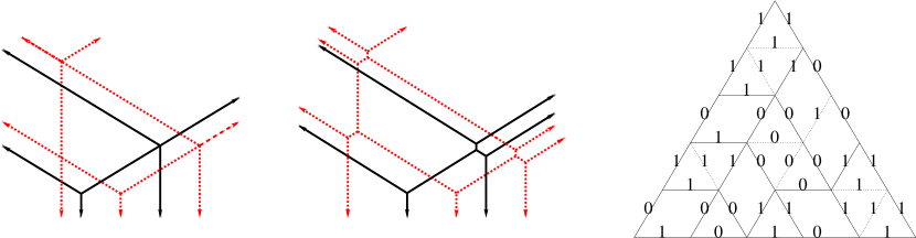
Figure 7. A clockwise overlay, a deformation of its constituents to nondegenerate honeycombs, and the puzzle built from that. The corresponding inequality on ${\tt BDRY}(5)$ is $\lambda_{1}+\lambda_{3}+\mu_{2}+\mu_{3}+\nu_{2}+\nu_{4}\geq 0$. Note that some edges of the original overlay have multiplicity 2, leading to repetitions along the boundary of the puzzle.

We can perturb $A^{\prime}$ and $B^{\prime}$ small amounts and vary the boundary coordinates of in arbitrary directions. This gives us a $(3n-2)$-dimensional family of possible boundaries containing our original point $\partial h$, all satisfying the stated inequality. By lemma 1, $h$ is in the interior of a facet determined by this inequality, which is the inequality $f_{P}\geq 0$. ∎

Call a clockwise overlay a witness to the facet it exhibits via lemma 4. This gives us a convenient way to exhibit facets.

Applying lemma 4 to lemma 3, we get

Theorem 3.

Let $\Phi$ be a regular facet of ${\tt BDRY}(n)$. Then there exists a puzzle $P$ such that $\Phi$ is the facet determined by $f_{P}\geq 0$, i.e. $\Phi={\tt BDRY}(n)\cap f_{P}^{-1}(0)$.

So each regular facet gives a puzzle, and each puzzle gives an inequality, that together with the list of chamber inequalities, determine ${\tt BDRY}(n)$ (and as we will see in section 6, this list is the same as Klyachko’s, itself the same as Horn’s).

But not every inequality is satisfied with equality on a facet. Define an inequality $f\geq 0$ on a polyhedron $\Pi$ to be essential if $f^{-1}(0)\cap\Pi$ is a facet of $\Pi$, and inessential if $f^{-1}(0)\cap\Pi$ is lower-dimensional. – equivalently, some positive multiple of it must show up in any finite list of inequalities that determine $\Pi$. For example, for a point in the plane to be in the first quadrant it is necessary and sufficient that it satisfy the inequalities $\{x\geq 0,y\geq 0,x+y\geq 0\}$, but the third inequality is only pressed at the origin, and can be omitted from the list). In the next section we will cut our list of inequalities on ${\tt BDRY}(n)$ down to the essential inequalities.

3.3. Independence of the chamber inequalities for $n>2$.

We have thus far ignored the chamber inequalities $\lambda_{i}\geq\lambda_{i+1}$ etc. on ${\tt BDRY}(n)$, focusing attention on the inequalities determining regular facets. We thank Anders Buch for pointing out to us the following subtlety that this perspective misses.

Theorem 4.

For $n>2$, the chamber inequalities on ${\tt BDRY}(n)$ are essential. For $n=2$, they are implied by the regular inequalities and the equality $\lambda_{1}+\lambda_{2}+\mu_{1}+\mu_{2}+\nu_{1}+\nu_{2}=0$.

Proof.

Consider a honeycomb $h$ satisfying $\lambda_{i}=\lambda_{i+1}$ for some $i$, but otherwise minimally degenerate; an example is in figure 8. (By $Z_{3}$ symmetry it is enough to consider the $\lambda$ case.)

Figure 8. A generic honeycomb over the chamber facet determined by $\lambda_{2}=\lambda_{3}$.

Note that there is only one nongeneric vertex, at the end of the multiplicity-two semiinfinite edge. It is straightforward to construct a similar such honeycomb for any $n$ and $i$.

We mimic the proof of proposition 1, in using the trading construction to exhibit a $(3n-2)$-dimensional family in ${\tt BDRY}(n)$ satisfying $\lambda_{i}=\lambda_{i+1}$. We can move the doubled edge wherever we like by translating the whole honeycomb. To trade the constant coordinates of any other two boundary edges, we use paths avoiding the bad vertex in $h$, which exist for $n>2$. This proves the first claim.

For $n=2$ we hit a snag – sometimes the only paths will go through the bad vertex. But we can check $n=2$ directly. The regular inequalities are

$$\lambda_{1}+\mu_{1}+\nu_{2}\geq 0,\quad\mu_{1}+\nu_{1}+\lambda_{2}\geq 0,\quad\nu_{1}+\lambda_{1}+\mu_{2}\geq 0.$$

Sum the first two, and subtract the equality $\lambda_{1}+\lambda_{2}+\mu_{1}+\mu_{2}+\nu_{1}+\nu_{2}=0$ to get $\mu_{1}-\mu_{2}\geq 0$. The other two inequalities are proved in ways symmetric to this one. ∎

4. Gentle loops vs. rigid puzzles

We have at this point an overcomplete list of inequalities, coming from puzzles; in section 6 we will see it is exactly that of H-R/T/K (which by [Hon1] is exactly that of Horn’s conjecture [H]). Our remaining goal is to cut down the list of inequalities to the essential set – those that determine facets of ${\tt BDRY}(n)$, rather than lower-dimensional faces.

To do this, we will shortly introduce the concept of a gentle loop in a puzzle, and prove two things:

• regular facets correspond 1:1 to puzzles without gentle loops

• a puzzle has no gentle loops if and only if it is rigid, i.e. is uniquely determined by its boundary conditions.

The first is remarkably straightforward, the second a bit more technical.

Cut a puzzle up along the interior edges that separate two distinct types of puzzle pieces; call the connected components of what remains the puzzle regions, coming in the three types $0$-region, $1$-region, and rhombus region. Define a region edge in a puzzle as one separating two distinct types of puzzle piece. Thus every region edge either separates a rhombus region from a $0$-region, or a $1$-region from a rhombus region. Orient these edges, so that $0$-regions are always on the left, and $1$-regions are always on the right. (Viewed as edges of the parallelograms, this orients them to point away from the acute vertices. Stated yet another way, they go clockwise around the $1$-regions, counterclockwise around the $0$-regions.) An example is in figure 9.

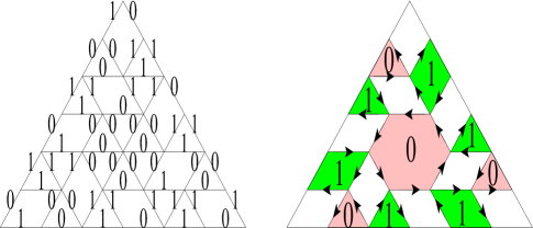
Figure 9. A puzzle, and its decomposition into regions, with region edges oriented. This is one of the two smallest examples with a gentle loop; it goes counterclockwise around the central hexagon.

Define a gentle path in a puzzle as a finite list of region edges, such that the head of each connects to the tail of the next, and the angle of turn is either $0^{\circ}$ or $60^{\circ}$, never $120^{\circ}$. Define a gentle loop as a gentle path such that the first and last edges coincide. The smallest puzzles with gentle loops are of size $6$; the one in figure 9 is one of the only two of that size.

(For this definition we did not really need to introduce puzzle regions, only region edges. We will need the regions themselves in section 5.)

To better understand gentle paths, we need to know the possible local structures of a puzzle around an interior vertex, which are straightforward to enumerate. Clockwise around a lattice point in a puzzle, we meet one of the following (see figure 10 for examples of each):

• six triangles of the same type

• four rhombi at acute, obtuse, acute, obtuse vertices

• three triangles of the same type, then two rhombi

• some $0$-triangles, an acute rhombus vertex, some $1$-triangles, and an obtuse rhombus vertex.

Only the latter two have region edges. This fourth type we call a rake vertex of the puzzle. (The reason for the terminology will become clearer in lemma 5.)

Figure 10. The possible local structures of a puzzle near an interior vertex, up to rotation and puzzle duality. The region edges incident on the vertex are oriented. This makes visible a “traffic-planning” mnemonic about gentle turns: any turn off a straightaway onto side roads is gentle, whereas there are no gentle on-ramps onto straightaways.

From this list, one sees easily that puzzle regions are necessarily convex: traversing their boundaries clockwise, one never turns left. In particular rhombus regions are necessarily parallelograms.

4.1. Puzzles have either witnesses or gentle loops.

Let $P$ be a puzzle constructed from a clockwise overlay $A\oplus B$ of two generic honeycombs, as in lemma 4. A gentle path in $P$ is in particular a sequence of puzzle edges, each successive pair sharing a vertex; there is a corresponding sequence of edges in $A\oplus B$, each successive pair being sides of the same region.

Proposition 2.

Let $A\oplus B$ be a clockwise overlay of two generic honeycombs, $P$ the corresponding puzzle (as in theorem 3), $\gamma=(\gamma_{1},\ldots,\gamma_{m})$ a gentle path in $P$, and $\tilde{\gamma}$ the corresponding sequence of edges in $A\oplus B$. Then the edge $\tilde{\gamma}_{1}$ is strictly longer than the edge $\tilde{\gamma}_{m}$.

Proof.

It is enough to prove it for gentle paths of length two, and then string the $m-1$ inequalities together. In figure 11 we present all length two paths (up to rotation and dualization), and the corresponding pairs of edges in an overlay. In each case the angles around the associated region force the strict inequality.

Figure 11. Gentle turns (through the latter two diagrams in figure 10) and the associated pairs of edges in a generic witness, up to rotation and dualization. Note that in each of the four gentle paths shown, the initial edge is necessarily longer than the terminal edge. Dualization flips the pictures, and exchanges $0$ for $1$, giving the same geometric inequality.

∎

Corollary.

Let $P$ be a puzzle with a gentle loop. Then $P$ does not arise from a clockwise overlay (“no witnesses”), and the inequality $P$ gives on ${\tt BDRY}(n)$ is inessential.

Proof.

If $P$ arises from a clockwise overlay $A\oplus B$, we can perturb $A$ and $B$ a bit to make them generic (as in the proof of theorem 3). Recall that a gentle loop is a gentle path whose first and last edges agree. Then by the proposition the corresponding edge in $A\oplus B$ is strictly longer than itself, contradiction.

By the contrapositive of lemma 3, $P$’s inequality is inessential. ∎

We now show that, conversely, gentle loops are the only obstructions to having witnesses. In other words, if a puzzle contains no gentle loops, then one can construct a witness $h$. The coming proposition 3 is inspired by the Wiener path integral, in which a solution to a PDE at a point $x$ is constructed as the sum of some functional over all possible paths from $x$ to the boundary. In our situation the role of the PDE is played by the requirement that the edges around a region of $h$ close up to form a polygon. This construction will give a witness to the puzzle provided that the number of gentle paths is finite, or equivalently if there are no gentle loops.

Lemma 5.

Let $P$ be a puzzle without gentle loops, and $v$ a rake vertex, as in figure 12, where four region edges meet. Call the east edge on $v$ the handle and the west edges the tines. Then the number of gentle paths starting at each of those four edges and terminating at the boundary is $a+b$ from the handle, $a$ from the two outer tines, and $b$ from the inner tine, for some $a,b\in{\mathbb{N}}$.

Figure 12. Every vertex of a puzzle region, interior to a puzzle, looks like a rake (up to rotation and reflection). This one has the “handle” on the right, and the three “tines” on the left.

Proof.

Of the two outer tines of the rake, one points toward the vertex, one points away. Every gentle path starting at the inward-pointing tine goes into the outward-pointing tine (to turn into the middle tine would not be gentle), and conversely every path from the outward-pointing can be extended; this is why they both have $a$ gentle paths to them for some $a\in{\mathbb{N}}$.

The gentle paths starting at the handle go either into the middle tine, or the outward-pointing outer tine. So if $b\in{\mathbb{N}}$ gentle paths start from the middle tine, $a+b$ start from the handle. ∎

We will use an equivalent geometrical statement: these numbers $a,b,a,a+b$ form the side lengths of a trapezoid in the triangular lattice.

Proposition 3.

Let $P$ be a puzzle of size $n$ with no gentle loops. Then there exists a clockwise overlay $h=A\oplus B$ such that the puzzle that theorem 3 associates to $h$ is $P$. Therefore by lemma 4, the inequality defined by the puzzle determines a facet of ${\tt BDRY}(n)$.

Moreover, in this witness $h$ every bounded nonzero edge of $A$ crosses a bounded nonzero edge of $B$, and vice versa.

We do this by direct construction. One example to follow along with is the left honeycomb in figure 7, whose regions are indeed all trapezoids.

Proof.

First note that for this purpose, it is enough to specify a honeycomb up to translation. To do that, it is enough to specify the lengths and multiplicities of the bounded edges, and say how to connect them. Not every specification works – the vertices have to satisfy the zero-tension condition of [Hon1], and the vector sum of the edges around a region must be zero.

To specify a clockwise overlay, we must in addition two-color the edges “$A$” and “$B$”, and make such edges only meet at crossing vertices, such that the colors alternate $A,B,A,B$ when read clockwise around each crossing vertex.

We now build a clockwise overlay $h$ as a sort of graph-theoretic dual of $P$ – one vertex for each puzzle region of $P$, one bounded edge for each region edge of $P$ (almost – two region edges on the same boundary of a region determine the same edge of $P$), one semiinfinite edge for each exterior edge of $P$. If $e_{h}$ is a bounded edge of $h$ corresponding to a region edge $e_{P}$ of $P$, then $e_{h}$

• is perpendicular to $e_{P}$

• is labeled $A$ or $B$ depending on whether $e_{P}$ is adjacent to a $1$ or $0$ region

• has multiplicity equal to the length of $e_{P}$

• has length equal to the number of gentle paths starting at $e_{P}$ and ending on the boundary of $P$.

This last number is finite exactly because there are no gentle loops.

The vertices of $h$ are zero-tension because the vector sum of the edges around a region in $P$ is zero. The regions in $h$ are all trapezoids, dual to the meeting of four regions in $P$ at rakes, and close up by lemma 5.

For the second statement, note that no edge of $h$ connects two distinct vertices in the same honeycomb, because the corresponding region edge in $P$ does not bound two regions of the same type. ∎

The witnesses produced by this construction seem so minimal and natural that we are tempted to christen them “notaries”. It would be interesting if there are correspondingly canonical witnesses in the Hermitian matrix context.

Together, this proposition 3 and the corollary to proposition 2 prove

Theorem 5.

There is a $1:1$ correspondence between $n$-puzzles without gentle loops and regular facets of ${\tt BDRY}(n)$, given by the assignment $P\mapsto``f_{P}\geq 0^{\prime\prime}$.

At this point we have a complete, combinatorial characterization of the regular facets of ${\tt BDRY}(n)$ – they correspond one-to-one to puzzles of size $n$ with no gentle loops. However, to better tie in to Belkale’s result we need to characterize such puzzles in terms of rigidity. One direction (Belkale’s) is the following theorem, the other to come in the next subsection.

Theorem 6.

Let $P$ be a puzzle with no gentle loops. Then $P$ is rigid. In particular (by theorem 5), the set of rigid puzzles of size $n$ gives a complete set of inequalities determining ${\tt BDRY}(n)$.

We use in this proof one result that does not come until proposition 4: the number of rhombi in a puzzle is determinable from the boundary conditions.

Proof.

Let $h=A\oplus B$ be a witness to $P$ produced during the proof of proposition 3. By slight perturbation of $A$ and $B$ to nondegenerate $A^{\prime}$ and $B^{\prime}$, small enough that no vertex of one crosses an edge of the other, we can create an $h^{\prime}$ whose only degenerate edges correspond to the rhombi in $P$. (One can modify the construction in proposition 3 to give such an $h^{\prime}$ directly, but it is not especially enlightening.)

Puzzles are easily seen to be determined by the set of their rhombi, and by proposition 4 (to come) the number of rhombi in a puzzle is determinable from the boundary conditions. So if $P$ is not rigid, so there exists another puzzle $Q$ with the same boundary, then this $Q$ has a rhombus that $P$ doesn’t. Then by its definition as a sum of edge-lengths, $f_{Q}(h^{\prime})>0$. But by theorem 2, $f_{Q}(h^{\prime})=f_{P}(h^{\prime})=0$, contradiction. ∎

One way to think about this is that if a puzzle inequality can be “overproved,” there being two distinct puzzles $P,Q$ giving the same inequality $f_{P}=f_{Q}\geq 0$, then the inequality is inessential.

(We will prove a stronger version of this result, in theorem 8.)

4.2. Breathing gentle loops.

It remains to be shown that puzzles with gentle loops are not rigid. The proof of this is very direct; given a sufficiently nice gentle loop $\gamma$ in a puzzle $P$, we will modify $P$ in a radius-$1$ neighborhood of $\gamma$ to get a new puzzle $P^{\prime}$ agreeing with $P$ outside that neighborhood, in particular on the boundary. The technical part comes in showing that minimal gentle loops are “sufficiently nice.”

Define the normal line to a vertex $v$ along a gentle path $\gamma$ to be a pair of edges attached to $v$ such that

• they are $180^{\circ}$ apart

• neither is in $\gamma$

• neither cuts through the middle of a rhombus puzzle piece.

Checking the four cases in figure 11, one sees that a normal line exists uniquely at each $v$. Note that the half of the normal line connected to the left side of $\gamma$ is always labeled $0$, and the right half always $1$.

We haven’t needed to speak of the distance between two puzzle vertices before; define it to be the graph-theoretic distance, where the graph in question is made from the lattice triangle’s vertices and edges (not just the edges appearing in the puzzle).

Lemma 6.

Let $P$ be a puzzle with a gentle loop $\gamma$, such that the only pairs of $\gamma$-vertices that are at distance $1$ in the puzzle are consecutive in $\gamma$. (In particular, the loop does not cross itself.) Then there exists a different puzzle $P^{\prime}\neq P$ that agrees with $P$ on any edge not touching $\gamma$.

Proof.

Let $N\gamma$ denote the radius-$1$ neighborhood of $\gamma$, i.e. the set of pieces of $P$ with a vertex on $\gamma$. By the condition about nonconsecutive vertices, this neighborhood doesn’t overlap itself, i.e. every edge connected to $\gamma$ (but not in $\gamma$) is connected to a unique vertex of $\gamma$.

Cut $N\gamma$ up along its normal lines. It is easy to check that it falls into only four kinds of “assemblages” up to rotation, listed in figure 13.

Figure 13. The four assemblages possible when a neighborhood of a gentle path is cut along normal lines (here drawn dashed). These have been rotated to make the gentle path point East.

Notice that for each assemblage, there is a unique other of the same shape, but rotated $180^{\circ}$. This pairs up the two triangular assemblages, the parallelograms each being self-matched. The crucial observation to make is that two matching assemblages have the same labels on the boundary (away from the normal lines).

In particular, if we simultaneously replace each assemblage in $N\gamma$ by the other one with the same shape, the new collection fits together (because all the normal lines have been reversed), fits into the rest of the original puzzle (because the labels on the boundary are the same), and gives a new gentle loop running in the opposite direction. ∎

We call this operation breathing the gentle loop, for reasons explained at the end of section 5. An example is given in figure 14.

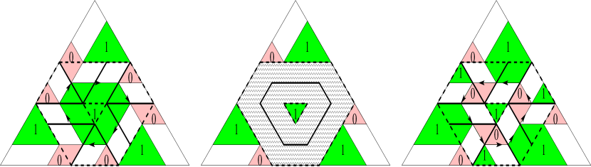
Figure 14. The left figure has a gentle loop running clockwise, with its neighborhood broken along normal lines into assemblages, as indicated. Removing that neighborhood gives the middle figure, and filling it in with each assemblage replaced by its match gives the right figure, which has a gentle loop running counterclockwise.

(In fact the new puzzle constructed this way is unique, and breathing the new gentle loop reproduces the original puzzle.)

Theorem 7.

If a puzzle has gentle loops, it is not rigid.

We will cut down the cases considered in this theorem using the following lemma, easily checked from figure 11:

Lemma 7.

If a 2-step gentle path $(\gamma_{1},\gamma_{2})$ in a puzzle $P$ turns while passing through a vertex (as opposed to going straight), there is another path $(\gamma_{1}^{\prime},\gamma_{2})$ turning from the opposite direction.

Proof of theorem 7.

We will show that minimal gentle loops satisfy the condition of lemma 6.

First we claim that minimal gentle loops do not self-intersect. Let $\gamma$ be a gentle loop that does self-intersect, and let $v$ be a vertex occurring twice on $\gamma$ such that the two routes through $v$ are different. (If there is no such $v$, then $\gamma$ is just a repeated traversal of a loop that does not self-intersect.) There are ${3\choose 2}=3$ local possibilities, corresponding to choosing two of the rightmost three gentle paths in figure 11; in each one we can break and reconnect the gentle loop to make a shorter one, contradicting minimality.

Second (and this is the rest of the proof) we claim that minimal gentle loops do not have nonconsecutive vertices at distance $1$. If $\gamma$ is a counterexample, then there exists an edge $E\notin\gamma$ connecting two points on $\gamma$. (This $E$ is just an edge in the lattice, not necessarily in the puzzle $P$ – it may bisect a rhombus of $P$ or whatever.) Removing the endpoints of $E$ from $\gamma$ separates $\gamma$ into two arcs; call the shorter one the minor arc and the longer the major arc. (If they are the same length make the choice arbitrarily.) Choose $E$ such that the minor arc is of minimal length.

For the remainder we assume (using puzzle duality if necessary) that the gentle loop is clockwise. We now analyze the local picture near $E$, which for purposes of discussion we rotate to horizontal so that the minor arc starts at the west vertex of $E$, and ends at the east vertex. This analysis proceeds by a series of reductions, pictured in figure 15.

Figure 15. The steps of theorem 7. The dashed lines indicate possible edges at each step 1-4, the solid lines definite ones.

1. The first edge of the minor arc goes either west, northwest, or northeast (to have room for a gentle turn from the major arc); likewise, the last edge goes either southeast, southwest, or west.

2. If the first edge of the minor arc went northeast, we could shift $E$ to $E^{\prime}$ connecting the second vertex of the minor arc to the last vertex, contradicting the assumption that the minor arc was minimal length. So in fact the first edge goes west or northwest, the last southwest or west (by the symmetric argument).

3. We now involve the major arc. Its last edge goes northwest or northeast. If it goes northeast, then the first edge of the minor arc goes northwest (for gentleness). But then by lemma 7 $E$ is oriented west; therefore we could shorten $\gamma$ to a loop that used $E$, contradicting $\gamma$’s assumed minimality. So the last edge of the major arc goes northwest.

4. Therefore the first edge of the major arc goes southeast (since $\gamma$ doesn’t intersect itself), so the last edge of the minor arc goes southwest. But then lemma 7 says that $E$ is oriented east.

At this point the west vertex of $E$ has an oriented edge coming in from the southeast, one going out to the east, and another going out either west or northwest (at least). This matches none of the vertices (or their puzzle duals) in figure 10. The contradiction is complete; there was no such $E$. ∎

The following strengthening of theorem 6 was also observed experimentally by W. Fulton.

Theorem 8.

Let $P$ be a nonrigid puzzle. Then the face of ${\tt BDRY}(n)$ determined by $f_{P}=0$ lies on a chamber wall.

Proof.

If not, there exists a regular boundary $b\in{\tt BDRY}(n)$ such that $f_{P}(b)=0$. Let $h$ be a largest lift of $b$; by theorem 2 of [Hon1] $h$ is simply degenerate. Since $P$ is nonrigid, by theorem 6 it has a gentle loop; a minimal such loop $\gamma$ is breathable, by the proof of theorem 7. Let $P^{\prime}$ be the result of breathing $P$ along $\gamma$.

We claim that some rhombus $\rho^{\prime}$ of $P^{\prime}$ overlaps some rhombus $\rho$ of $P$ in a triangle. To see this, divide $\gamma$ up along its normal lines into the assemblages of lemma 6, figure 13. At least one such assemblage must be a triangle, for otherwise the loop can not close up. (In fact there must be at least six triangles.) When we breathe the loop, the rhombus $\rho$ in the original assemblage in $P$ overlaps the rhombus $\rho^{\prime}$ in the new assemblage in $P^{\prime}$ in a triangle.

Dually, the edges of the honeycomb tinkertoy $\tau_{n}$ corresponding to those two rhombi meet at a vertex.

Since $f_{P}(h)=f_{P}^{\prime}(h)=0$, and they are defined as the sum of certain edge-lengths of $h$, all those edges of $h$ must be length zero. Therefore, the two adjacent edges in $h$ corresponding to $\rho$ and $\rho^{\prime}$ are length zero. But then $h$ is not simply degenerate, contradiction. ∎

At this point we have a second characterization of the regular facets of ${\tt BDRY}(n)$; they correspond to rigid puzzles. For our final characterization we need to involve the other life of puzzles, which is in computing Schubert calculus of Grassmannians.

5. Puzzle inflation, rhombi, and Schubert calculus

We start with an “inflation” operation on puzzles, taking a puzzle $P$ and a natural number $N$ to a new puzzle $N\cdot P$:

Lemma 8.

Let $P$ be a puzzle of size $n$. For $N\in{\mathbb{N}}$, define $N\cdot P$ to be the puzzle whose puzzle regions are in correspondence with $P$’s, and glued together the same way, but every edge labeled $1$ has been stretched by the factor $N$. Then $N\cdot P$ is a well-defined puzzle. In addition, $N\cdot P$ is rigid if and only if $P$ is rigid.

An example is in figure 16.

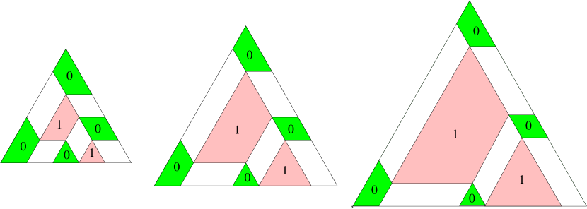
Figure 16. A puzzle $P$ broken into regions, $2\cdot P$, and $3\cdot P$.

Proof.

To see that $N\cdot P$ is a well-defined puzzle, we need to check that each new region is well-defined – that traversing its boundary we return to where we started. For $0$-regions there is nothing to show, for $1$-regions the whole region is inflated by the factor $N$, and for rhombus regions two opposite sides of the parallelogram are stretched.

There is an evident correspondence between gentle loops in $P$ and gentle loops in $N\cdot P$, so by theorems 6 and 7 they are either both rigid or neither is. ∎

Our principal use of this will be the deflation $0\cdot P$ of a puzzle.

Proposition 4.

Let $P$ be an $n$-puzzle, such that one side has $r$ $1$-edges. Then the other two sides also have $r$ $1$-edges, and the puzzle consists of

• $r^{2}$ $1$-triangles, of which ${r+1\choose 2}$ are right-side-up and ${r\choose 2}$ are upside-down

• $(n-r)^{2}$ $0$-triangles, of which ${(n-r)+1\choose 2}$ are right-side-up and ${n-r\choose 2}$ are upside-down

• $r(n-r)$ rhombi.

Since we already know every facet comes from a puzzle (theorem 3), this implies Horn’s results on the structure of the inequalities determining facets, explained in subsection 3.1.

Proof.

The deflation of $P$ is an $(n-r)$-puzzle consisting only of $0$-triangles, letting us count the number of $0$-triangles in the original puzzle (namely, $(n-r)^{2}$) and also the number of $0$-edges on the three sides (namely, $n-r$). By deflating the dual puzzle, one can count there to be $r^{2}$ $1$-triangles. The remaining area is $n^{2}-r^{2}-(n-r)^{2}=2r(n-r)$ in units of triangle, and all that is available are rhombi which each use up 2. ∎

We now prove that puzzles compute Schubert calculus on Grassmannians (our reference for the latter is [F2]), as stated in the introduction. Recall that we index Schubert classes in $H^{*}({\rm Gr}_{r}({\mathbb{C}}^{n}))$ by $n$-tuples consisting of $r$ ones and $n-r$ zeroes.

What we will actually prove is that the puzzle rule is equivalent to the honeycomb rule from [Hon1]. (A direct proof will appear in [KT1], in turn giving an independent proof of the honeycomb rule.) First we need a lemma on honeycombs:

Lemma 9.

Let $h$ be a honeycomb with boundary coordinates $(\lambda,\mu,\nu)\in({\mathbb{R}}^{n})^{3}$ on the Northwest, Northeast, and South sides, each a weakly decreasing list of real numbers. Then

1. The first coordinate of any vertex of $h$ is in the interval $[\lambda_{n},\lambda_{1}]$. (Likewise second coordinate in $[\mu_{n},\mu_{1}]$, third coordinate in $[\nu_{n},\nu_{1}]$.)

2. The third coordinate of any vertex is in the interval $[-\lambda_{1}-\mu_{1},-\lambda_{n}-\mu_{n}]$.

3. If $\lambda_{i},\mu_{i},-\nu_{i}\in[0,M]$ for all $i=1\ldots n$, then all of $h$’s vertices are in the triangle with vertices $(0,0,0),(M,0,-M),(0,M,-M)$.

Proof.

1. Follow a path in the honeycomb, going Northwest whenever possible, Southwest when not, eventually coming out on an edge with constant coordinate $\lambda_{i}\leq\lambda_{1}$. Each Southwest sojourn increases the first coordinate, and each Northwest leaves it unchanged, so the original first coordinate must have been at most $\lambda_{1}$. Replacing “Southwest” with “North” gives the opposite inequality. The other two coordinates come from rotating this proof $\pm 120^{\circ}$.

2. Since the sum of the three coordinates is zero by definition, the third one can be bounded in terms of the first two.

3. This is just a special case of (1). ∎

Theorem (theorem 1 from the introduction).

Let $\pi,\rho,\sigma$ be three strings of $r$ ones and $n-r$ zeroes. Then the number of puzzles with $\pi,\rho,\sigma$ clockwise around the boundary is the Schubert intersection number $\int_{{\rm Gr}_{r}({\mathbb{C}}^{n})}S_{\pi}S_{\rho}S_{\sigma}$.

Equivalently, write $S_{\pi}S_{\rho}=\sum_{\tau}c_{\pi\rho}^{\tau}S_{\tau}$. The the number of puzzles with $\pi,\rho$ on the NW and NE boundaries, and $\tau$ on the South boundary, all written left to right, is the structure constant $c_{\pi\rho}^{\tau}$.

Proof.

We prove the second statement: the first follows from the second, since $\int_{{\rm Gr}_{r}({\mathbb{C}}^{n})}S_{\pi}S_{\tau}$ is $1$ if $\pi$ is the reversal of $\tau$, $0$ otherwise.

The structure constants for multiplication of Schubert classes are well known to also be the structure constants for tensor products of polynomial representations of ${{GL_{n}({\mathbb{C}})}}$ (the first to observe this seems to be Ehresmann; see [F2] or [KT2]). The precise statement is as follows. Let $\lambda_{i}$ be the number of $0$s after the $i$th $1$ in $\pi$, so $\lambda_{1}\geq\lambda_{2}\geq\ldots\geq\lambda_{r}$, and $\lambda$ is a partition of the number of inversions of $\pi$. Likewise construct $\mu$ from $\rho$, and $\nu$ from $\tau$. Then

$$c_{\pi\rho}^{\tau}=\dim{\rm Hom}_{{{GL_{n}({\mathbb{C}})}}}(V_{\nu},V_{\lambda}{\otimes}V_{\mu}).$$

This latter can be calculated using honeycombs, as proved in [Hon1]; it is the number of honeycombs with boundary coordinates $(\lambda_{1}\geq\ldots\geq\lambda_{r})$ on the Northwest side, $(\mu_{1}\geq\ldots\geq\mu_{r})$ on the Northeast, and $(-\nu_{r}\geq\ldots\geq-\nu_{1})$ on the South.

We now construct a map from our puzzles to these honeycombs. To create a honeycomb from a puzzle is a three-step process (follow along with the example in figure 17):

1. Place the puzzle in the plane ${\mathbb{R}}^{3}_{\sum=0}$ such that the bottom right corner is at the origin, and turn it $30^{\circ}$ counterclockwise.

2. At each boundary edge labeled $1$, attach a rhombus (outside the puzzle), then another (parallel to the first), and repeat forever. Fill in the rest of the plane with $0$-triangles.

3. Deflate the extended puzzle, keeping the right corner at the origin. The honeycomb’s vertices then come from the deflated $1$-regions, and the honeycomb’s edges come from the deflated rhombus regions, with the multiplicity on the edge coming from the thickness of the original rhombus region.

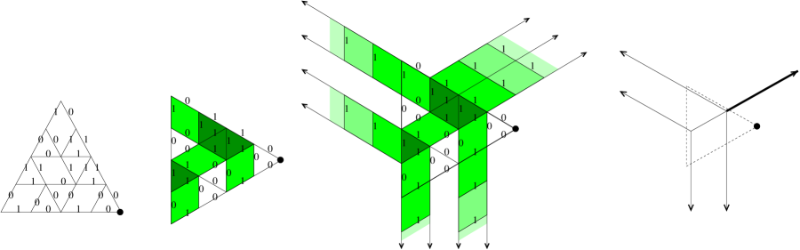
Figure 17. A puzzle, and the three stages in creating a honeycomb from it. Regions with $1$s on their boundary are shaded, and then deflated. The origin $(0,0,0)$ is indicated in each figure by a heavy dot.

The resulting diagram obviously has finitely many vertices, all edges in triangular-coordinate directions, and semiinfinite edges only going NW/NE/S (coming from the $1$-edges on the boundary of the original puzzle). The remaining condition for it to be the diagram of a honeycomb is that each vertex have zero total tension; this is equivalent to the fact that the original $1$-region was a closed polygon.

To see that this is a bijection, we construct the inverse map. Start with a honeycomb computing $c_{\pi\rho}^{\tau}$. By part 2 of lemma 9, it fits inside the triangle with vertices $(0,0,0),(n-r,0,r-n),(0,n-r,r-n)$. Inflate each edge of the honeycomb intersected with the triangle to a rhombus region, the thickness given by the multiplicity of the edge, and each vertex to a polygon of $1$-triangles, the lengths of the edges of the polygon given by the multiplicities of the edges at the vertex. The result is a puzzle with boundary $\lambda,\mu,\nu$. ∎

In [KT1] will appear an alternate proof of this theorem not using honeycombs, which shows also that puzzles compute $T$-equivariant cohomology of Grassmannians, when one includes an additional “equivariant puzzle piece”.

We conclude this section with some observations.

1. This intersection number problem has 12 manifest symmetries; $3!$ from permuting $\pi,\rho,\sigma$, and $2$ from the duality diffeomorphism ${\rm Gr}_{r}({\mathbb{C}}^{n}){\cong}{\rm Gr}_{n-r}({\mathbb{C}}^{n})$. As with honeycombs and Berenstein-Zelevinsky patterns, only half of these are manifest in the rule; rotating the puzzles gives the even permutations of $\pi,\rho,\sigma$, and puzzle duality gives the composition of Grassmann duality with the odd permutation $\pi\leftrightarrow\sigma$. None of these are directly visible in the Littlewood-Richardson rule (for a deeper discussion of this, see [KT2]).

2. This theorem makes possible a (rather forced) duality on honeycombs, as already observed in [GP, Hon1]: pick a triangle containing the honeycomb, inflate to a puzzle, apply puzzle duality, and deflate back to a new honeycomb, the total effect being to exchange vertices for regions and vice versa. Unfortunately this depends on the choice of triangle, and only works for integral honeycombs. This is quite different from the much more natural duality on honeycombs that comes from flipping them over, $(x,y,z)\mapsto(-y,-x,-z)$.

3. In [Hon1] we defined a way of locally modifying a honeycomb in the vicinity of a loop through nondegenerate vertices, which was also called breathing. It is easy to check that any breathing operation on honeycombs is, under the deflation correspondence above, the deflation of a gentle-loop breathing on a puzzle. (The reverse is not true: gentle-loop breathing of puzzles is a strict generalization.)

4. Note that this connection of puzzles and honeycombs is completely different from the one in theorem 3, and serves as a combinatorial explanation of the recursive nature of Horn’s list of inequalities. To recapitulate the chain of reasoning involved: first one studies extremal $n$-honeycombs (as we did in section 3), and from an extremal honeycomb, which is necessarily an overlay of a $r$-honeycomb and an $(n-r)$-honeycomb, one constructs a puzzle encoding the pattern of overlay. That puzzle then deflates to a $r$-honeycomb, necessarily integral. Therefore inequalities on $n$-honeycombs can be “blamed” on integral $r$-honeycombs. This is not recursive until one knows that honeycombs exist with given integral boundary conditions if and only if integral honeycombs exist with the same boundary; this was (the honeycomb version of) the saturation conjecture, proved in [Hon1].

6. Replacing puzzles by Schubert calculus

So far we have used puzzles to give inequalities on the boundaries of honeycombs. In this section we replace puzzles by Schubert calculus, and honeycombs by zero-sum Hermitian triples, to formulate puzzle- and honeycomb-free versions of most of our results. The only casualty is the characterization of rigid puzzles as those without gentle loops; but this too has an application, in proving a conjecture of W. Fulton.

First we recall the connection of honeycombs to Hermitian matrices: Let $(\lambda,\mu,\nu)\in({\mathbb{R}}^{n})^{3}$ be three weakly decreasing lists of real numbers. Then there exists a honeycomb with boundary coordinates $(\lambda,\mu,\nu)$ if and only if there exists a triple of Hermitian matrices $(H_{\lambda},H_{\mu},H_{\nu})$ with spectra $\lambda,\mu,\nu$ and adding to the zero matrix. This follows from [Hon1] and [Kl]; we make a more precise statement in the appendix, replacing Klyachko’s argument with more direct use of the relation between geometric invariant theory quotients and symplectic quotients.

Corollary.

Avoiding direct mention of honeycombs and puzzles, we have

1. [T, HR, Kl] If $S_{\pi},S_{\rho},S_{\sigma}$ are three Schubert classes on ${\rm Gr}_{r}({\mathbb{C}}^{n})$ such that $\int_{{\rm Gr}_{r}({\mathbb{C}}^{n})}S_{\pi}S_{\rho}S_{\sigma}>0$, then for any triple $H_{\lambda},H_{\mu},H_{\nu}$ of $n\times n$ Hermitian matrices with zero sum and spectra $\lambda,\mu,\nu$ (written in decreasing order) respectively, we have the inequality

   $$\sum_{i=1}^{n}\pi_{i}\lambda_{i}+\rho_{i}\mu_{i}+\sigma_{i}\nu_{i}\leq 0.$$

2. [Kl] This list of inequalities on the spectra is sufficient for the existence of such a triple.

3. [Be] If $S_{\pi},S_{\rho},S_{\sigma}$ are three Schubert classes on ${\rm Gr}_{r}({\mathbb{C}}^{n})$ such that $\int_{{\rm Gr}_{r}({\mathbb{C}}^{n})}S_{\pi}S_{\rho}S_{\sigma}>1$, then the corresponding H-R/T/K inequality is inessential…

4. …and equality can only occur when $(\lambda,\mu,\nu)$ are not all regular.

5. If $S_{\pi},S_{\rho},S_{\sigma}$ are three Schubert classes on ${\rm Gr}_{r}({\mathbb{C}}^{n})$ such that $\int_{{\rm Gr}_{r}({\mathbb{C}}^{n})}S_{\pi}S_{\rho}S_{\sigma}=1$, then the corresponding H-R/T/K inequality is essential.

Proof.

These are theorem 1 combined with

1. theorem 2 (the inequality is reversed because we are summing over $1$s here instead of $0$s)

2. theorem 3

3. theorem 6

4. theorem 8

5. theorems 5 and 7.

∎

We have another puzzle-free application of theorem 1:

6.1. Fulton’s conjecture.

In a private communication, W. Fulton proposed the following

Conjecture.

Let $\lambda,\mu,\nu\in({\mathbb{Z}}^{n})^{3}$ be a triple of dominant weights for ${{GL_{n}({\mathbb{C}})}}$, and $V_{\lambda},V_{\mu},V_{\nu}$ the corresponding irreducible representations. If $V_{\nu}$ occurs exactly once as a constituent of $V_{\lambda}{\otimes}V_{\mu}$, then $\forall N\in{\mathbb{N}}$, $V_{N\nu}$ occurs exactly once as a constituent of $V_{N\lambda}{\otimes}V_{N\mu}$.

It is interesting to compare this to the saturation conjecture (proven in [Hon1]). Saturation says that if a polytope of honeycombs with fixed integral boundary is nonempty, the polytope contains at least one lattice honeycomb. The present conjecture is sort of a next step: its contrapositive says that if a polytope of honeycombs with fixed integral boundary is not only nonempty but positive-dimensional, the polytope contains at least two lattice honeycombs.

We need one additional construction in order to prove this conjecture: the dual inflation of a puzzle by a factor $M$, defined as dualizing the puzzle, $M$-inflating, then dualizing again. This amounts to thinking of the inflation of a puzzle in terms of the $0$-edges instead of the $1$-edges.

Proof of Fulton’s conjecture..

Let $\det=(1,1,\ldots,1)$ denote the high weight of the determinant representation, and $c_{\lambda\mu}^{\nu}$ denote the number of times $V_{\nu}$ appears in $V_{\lambda}{\otimes}V_{\mu}$. Then using the equality

$$c_{\lambda\mu}^{\nu}=c_{\lambda+L\det,\,\mu+M\det}^{\nu+(L+M)\det},$$

we can reduce to the case that $\lambda$ and $\mu$ are nonnegative (so, high weights of polynomial representations). Therefore $\nu$ is also nonnegative, for otherwise $c_{N\lambda,N\mu}^{N\nu}$ would be zero for all $N\in{\mathbb{N}}$.

From there, we can use theorem 1 to convert to a Schubert problem, i.e. counting puzzles rather than honeycombs. One then has to check that rescaling a honeycomb by the factor $N$ corresponds to dual-inflation on puzzles.

Since the original honeycomb $h$ is rigid, so too is the corresponding puzzle $P$, therefore by lemma 8 so too is the dual inflation of $P$ by the factor $N$, and therefore so is $N\cdot h$. ∎

6.2. $(N,M)$-inflation and non-polynomiality.

Define the $(N,M)$-inflation of a puzzle by $N$-inflating it, and then $M$-dual-inflating it (these operations commute).

Note that this descends to a well-defined notion of the $(N,M)$-inflation of a boundary condition on a puzzle, and as such one can study the functions

$$f(N,M):=\#\hbox{puzzles with boundary $(N,M)\cdot\pi,\,(N,M)\cdot\rho,\,(N,M)\cdot\sigma$}$$

for fixed initial boundary conditions $\pi,\rho,\sigma$. Because of the connections of puzzles to honeycombs and thereby to sections of a line bundle over $({{GL_{n}({\mathbb{C}})}}/B)^{3}//{{GL_{n}({\mathbb{C}})}}$ (see the appendix), one can show that $f(N,M)$ is a polynomial function of one argument when the other is held fixed.

Taken together, though, the growth is usually exponential; the reader may enjoy showing that for $\pi=\rho=\sigma=010101$ (as in figure 9), $f(N,M)={N+M\choose N}$.

7. Summing more than three matrices

The cone ${\tt BDRY}(n)$, whose facets we have now completely determined, has a generalization for any $m\in{\mathbb{N}}$: the set of $m$-tuples of spectra

$${\tt BDRY}_{m}(n):=\bigg{\{}(\lambda_{i})_{i=1\ldots m}\quad:\quad\exists\{H_{i}\},\sum_{i}H_{i}=0\bigg{\}}$$

such that there exist $n\times n$ Hermitian matrices with those spectra adding to the zero matrix. (Again, this is equivalent to the corresponding $m$-fold tensor product problem.) Then ${\tt BDRY}_{3}(n)$ is just the cone ${\tt BDRY}(n)$ we’ve already determined, and ${\tt BDRY}_{1}(n),{\tt BDRY}_{2}(n)$ are uninteresting.

To study this cone for $m>3$ by the techniques in [Hon1] and this paper, we need to determine the corresponding honeycomb extension problem. We do this by factoring the problem: sum the first $m-2$ matrices and call the eigenvalues of that $\mu$, then see if $\mu$ goes with the last two spectra.

$${\tt BDRY}_{m}(n)=\bigg{\{}(\lambda_{i})_{i=1\ldots m}\quad:\quad\exists\mu,(\lambda_{1},\ldots,\lambda_{m-2},\mu^{*})\in{\tt BDRY}_{m-1}(n),(\mu,\lambda_{m-1},\lambda_{m})\in{\tt BDRY}_{3}(n)\bigg{\}}$$

(Here $\mu^{*}$ denotes $-\mu$, reversed so as to again be in decreasing order.) Repeat this factorization until everything is in terms of ${\tt BDRY}_{3}(n)={\tt BDRY}(n)$. Then we can think of ${\tt BDRY}_{m}(n)$ in terms of an $(m-2)$-tuple of honeycombs such that one boundary of each honeycomb anti-agrees with one boundary of the next. Define an $m$-ary honeycomb as exactly such an $(m-2)$-tuple.

Graphically, the easiest way to think about these is to draw the honeycombs in the same plane, half of them upside down, and very far from one another, as in figure 18. To get them far from one another we can add a large-enough constant $x$ to the coordinates. Note that we do not have to go beyond two dimensions, as is many people’s first guess about $m>3$ (or indeed $n>3$).

Figure 18. A honeycomb whose boundary lies in ${\tt BDRY}_{7}(n)$.

All the same techniques developed for $m=3$ go through without change. Define an $m$-ary puzzle as an $(m-2)$-tuple of puzzles (every other one upside down) that can be fitted together into a line, and call the individual puzzles the constituents of the $m$-ary puzzle. (Careful: these are not merely arrangements of puzzle pieces into a trapezoid/parallelogram; they satisfy the extra condition that no rhombus is allowed to cross from one constituent into the next.) On the Schubert calculus side, these count intersections of $m$ cycles in a Grassmannian. In figure 19 we give the famous count (two) of the number of lines touching four others in ${\mathbb{C}\mathbb{P}}^{3}$.

Figure 19. Given four generic lines in ${\mathbb{C}\mathbb{P}}^{3}$, exactly two lines touch all four. The gentle loops are drawn around the central hexagons.

A gentle path in an $m$-ary puzzle has essentially the same definition, with the only tricky point that it cannot include one of the edges joining one constituent puzzle to the next. With these definitions we have the analogous results:

Theorem 9.

Each $m$-ary puzzle gives a nonnegative functional on ${\tt BDRY}_{m}(n)$. The regular facets of ${\tt BDRY}_{m}(n)$ come precisely from the $m$-ary puzzles with no gentle loops. These $m$-ary puzzles are exactly the rigid ones, corresponding to $m$ Grassmannian Schubert cycles intersecting in a unique point.

Proof.

All the proofs go through without modification, except for one: we need to check that when we breathe a gentle loop in an $m$-ary puzzle using the loop-breathing lemma 6, we don’t introduce any rhombi that cross from one constituent puzzle to the next, for that would remove a boundary edge from a puzzle. But the edges separating constituents are obviously on normal lines to the gentle path, and the loop-breathing construction does not remove these edges. ∎

7.1. A representative example.

In figure 19 we exhibited two $4$-ary puzzles with the same boundary. By our theorems, we know that these have gentle loops, and determine the same true inequality

$$\lambda_{1}+\lambda_{3}+\mu_{1}+\mu_{3}+\nu_{1}+\nu_{3}+\pi_{1}+\pi_{3}\geq 0$$

on spectra of four Hermitian matrices with zero sum, but that this inequality is inessential.

8. Appendix: the equivalence of the definitions of ${\tt BDRY}(n)$

All the arguments in this paper study ${\tt BDRY}(n)$ purely in terms of its interpretation as the possible boundary conditions of honeycombs. In [Hon1], these are related to invariants in tensor products of ${{GL_{n}({\mathbb{C}})}}$-representations, which are turn related to Hermitian matrices in [Kl].

We include here a stronger result (which could already have been given in [Hon1]), replacing Klyachko’s argument by the Kirwan/Kempf-Ness theorem, allowing for a more precise result. While this involves some somewhat formidable machinery, its application really is a routine matter, and so we label the following a corollary.

Corollary (to theorem 4 of [Hon1]).

Let $(\lambda,\mu,\nu)\in({\mathbb{R}}^{n})^{3}$ be a triple of weakly decreasing $n$-tuples of reals. The volume (resp. real dimension) of the polytope of honeycombs in ${\tt HONEY}(\tau_{n})$ with boundary coordinates $(\lambda,\mu,\nu)$ is equal to the symplectic volume (resp. complex dimension) of the space of zero-sum Hermitian triples with these spectra modulo the diagonal action of $U(n)$. In particular, there exists such a honeycomb if and only if there exists such a zero-sum Hermitian triple.

Proof.

The machinery used here is geometric invariant theory, particularly the “geometric invariant theory quotients are symplectic quotients” theorem [MFK, chapter 8]. To begin with, take $(\lambda,\mu,\nu)$ integral, and consider the graded ring

$$R:=\bigoplus_{k}V_{k\lambda}{\otimes}V_{k\mu}{\otimes}V_{k\nu}.$$

By the Borel-Weil theorem, ${\rm Proj\,}R$ is a product of three (partial) flag manifolds as an algebraic variety, and from its induced projective embedding inherits a symplectic structure. By Kostant’s extension of Borel-Weil, it is symplectomorphic to the product of the $U(n)$ coadjoint orbits through $\lambda,$ $\mu,$ and $\nu$. We use the trace form on ${\mathfrak{u}}(n)$ to identify these with the corresponding isospectral sets of Hermitian matrices.

Now consider the invariant subring $R^{GL_{n}}$. By definition, ${\rm Proj\,}R^{GL_{n}}$ is the geometric invariant theory quotient of this product of three flag manifolds by the diagonal action of $GL_{n}$. By theorem 4 of [Hon1], the Hilbert function of this variety is the Erhart function of the polytope of honeycombs with boundary conditions $(\lambda,\mu,\nu)$. In particular its leading coefficient (resp. its degree), which as for any projective variety is the variety’s symplectic volume (resp. its complex dimension), is also the volume (resp. real dimension) of the polytope.

By the GIT/symplectic equivalence, this GIT quotient by $GL_{n}$ can alternately be constructed as a symplectic quotient by its maximal compact $U(n)$. This construction takes the zero level set of the $U(n)$ moment map – here the moment map is the sum of the three matrices – and quotients it by $U(n)$. Combining these results, we find that the symplectic volume (resp. complex dimension) of the moduli space of zero-sum Hermitian triples is the volume (resp. real dimension) of the polytope of honeycombs.

The same holds for rational triples $(\lambda,\mu,\nu)$ because both sides behave the same way under rescaling, and then for arbitrary triples because both sides are continuous. ∎

In particular (as Klyachko proves): an invariant tensor implies the existence of a zero-sum Hermitian triple, and a zero-sum Hermitian triple implies the existence of an invariant tensor in $V_{k\lambda}{\otimes}V_{k\mu}{\otimes}V_{k\nu}$ for some $k>0$. To go from there to $k=1$ is harder, requiring the saturation conjecture proved in [Hon1].

References

- [Be] P. Belkale, Local systems on for a finite set, Compositio Math. 129 (2001), no. 1, 67–86.
- [DW1] H. Derksen, J. Weyman, On the -stable decomposition of quiver representations, preprint available at http://www.math.lsa.umich.edu/~hderksen/preprint.html.
- [DW2] H. Derksen, J. Weyman, On the Littlewood-Richardson polynomials, preprint available at http://www.math.lsa.umich.edu/~hderksen/preprint.html.
- [F1] W. Fulton, Eigenvalues, invariant factors, highest weights, and Schubert calculus, Bull. Amer. Math. Soc. 37 (2000), 209-249.
- [F2] W. Fulton, Young tableaux. With applications to representation theory and geometry. London Mathematical Society Student Texts, 35. Cambridge University Press, Cambridge, 1997.
- [GP] O. Gleizer, A. Postnikov, Littlewood-Richardson coefficients via Yang-Baxter equation, math.QA/9909124, Internat. Math. Res. Notices no. 14 (2000), 741–774.
- [HR] U. Helmke, J. Rosenthal, Eigenvalue inequalities and Schubert calculus, Math. Nachr. 171, (1995), 207-225.
- [H] A. Horn, Eigenvalues of sums of Hermitian matrices, Pacific J. Math., 12 (1962), 225-241.
- [Hon1] A. Knutson, T. Tao, The honeycomb model of tensor products I: proof of the saturation conjecture, J. of Amer. Math. Soc, 12 (1999), no. 4, 1055-1090.
- [Kl] A.A. Klyachko, Stable vector bundles and Hermitian operators, IGM, University of Marne-la-Vallee preprint (1994).
- [K] A. Knutson, The symplectic and algebraic geometry of Horn’s problem, Linear Algebra and its Applications 319 (2000), no. 1-3, 61–81.
- [KT1] A. Knutson, T. Tao, Puzzles and (equivariant) cohomology of Grassmannians, in preparation.
- [KT2] A. Knutson, T. Tao, Puzzles, Littlewood-Richardson rings, and the legend of Procrustes, in preparation.
- [MFK, chapter 8] D. Mumford, J. Fogarty, F. Kirwan, Geometric invariant theory. Third edition. Ergebnisse der Mathematik und ihrer Grenzgebiete, Springer-Verlag, 1994.
- [T] B. Totaro, Tensor products of semistables are semistable, Geometry and Analysis on complex manifolds, World Sci. Publ. (1994), 242–250.