Holomorphic disks and three-manifold invariants: properties and applications

Abstract.

In [27], we introduced Floer homology theories $HF^{-}(Y,\mathfrak{s})$, $HF^{\infty}(Y,\mathfrak{s})$, $HF^{+}(Y,\mathfrak{t})$, $\widehat{HF}(Y,\mathfrak{s})$,and $HF_{\rm red}(Y,\mathfrak{s})$ associated to closed, oriented three-manifolds $Y$ equipped with a ${\mathrm{Spin}}^{c}$ structures $\mathfrak{s}\in{\mathrm{Spin}}^{c}(Y)$. In the present paper, we give calculations and study the properties of these invariants. The calculations suggest a conjectured relationship with Seiberg-Witten theory. The properties include a relationship between the Euler characteristics of $HF^{\pm}$ and Turaev’s torsion, a relationship with the minimal genus problem (Thurston norm), and surgery exact sequences. We also include some applications of these techniques to three-manifold topology.

1. Introduction

The present paper is a continuation of [27], where we defined topological invariants for closed oriented, three-manifolds $Y$, equipped with a ${\mathrm{Spin}}^{c}$ structure $\mathfrak{s}\in{\mathrm{Spin}}^{c}(Y)$. These invariants are a collection of Floer homology groups $HF^{-}(Y,\mathfrak{s})$, $HF^{\infty}(Y,\mathfrak{s})$, $HF^{+}(Y,\mathfrak{s})$, and $\widehat{HF}(Y,\mathfrak{s})$. Our goal here is to study these invariants: calculate them in several examples, establish their fundamental properties, and give some applications.

We begin in Section 2 with some of the properties of the groups, including their behaviour under orientation reversal of $Y$ and conjugation of its ${\mathrm{Spin}}^{c}$ structures. Moreover, we show that for any three-manifold $Y$, there are at most finitely many ${\mathrm{Spin}}^{c}$ structures $\mathfrak{s}\in{\mathrm{Spin}}^{c}(Y)$ with the property that $HF^{+}(Y,\mathfrak{s})$ is non-trivial.

In Section 3, we illustrate the Floer homology theories by computing the invariants for certain rational homology three-spheres. These calculations are done by explicitly identifying the relevant moduli spaces of flow-lines. In Section 4 we compare them with invariants with corresponding “equivariant Seiberg-Witten-Floer homologies”$HF_{{\rm to}}^{SW}$, $HF_{{\rm from}}^{SW}$, and $HF^{SW}_{{\rm red}}$ for the three-manifolds studied in Section 3, compare [21], [16].

These calculations support the following conjecture:

Conjecture 1.1.

Let $Y$ be an oriented rational homology three-sphere. Then for all ${\mathrm{Spin}}^{c}$ structures $\mathfrak{s}\in{\mathrm{Spin}}^{c}(Y)$ there are isomorphisms

$$HF_{{\rm to}}^{SW}(Y,\mathfrak{s})\cong HF^{+}(Y,\mathfrak{s}),\ \ HF_{{\rm from}}^{SW}(Y,\mathfrak{s})\cong HF^{-}(Y,\mathfrak{s}),\ \ HF^{SW}_{{\rm red}}(Y,\mathfrak{s})\cong HF_{\rm red}(Y,\mathfrak{s}).$$

After the specific calculations, we turn back to general properties. In Section 5, we consider the Euler characteristics of the theories. The Euler characteristic of $\widehat{HF}(Y,\mathfrak{s})$ turns out to depend only on homological information of $Y$, but the Euler characteristic of $HF^{+}$ has richer structure: indeed, when $b_{1}(Y)>0$, we establish a relationship between it and Turaev’s torsion function (c.f. Theorem 5.2 in the case where $b_{1}(Y)=1$ and Theorem 5.11 when $b_{1}(Y)>1$):

Theorem 1.2.

Let $Y$ be a three-manifold with $b_{1}(Y)>0$, and $\mathfrak{s}$ be a non-torsion ${\mathrm{Spin}}^{c}$ structure, then

$$\chi(HF^{+}(Y,\mathfrak{s}))=\pm\tau(Y,\mathfrak{s}),$$

where $\tau\colon{\mathrm{Spin}}^{c}(Y)\longrightarrow\mathbb{Z}$ is Turaev’s torsion function. In the case where $b_{1}(Y)=1$, $\tau(\mathfrak{s})$ is calculated in the “chamber” containing $c_{1}(\mathfrak{s})$.

For zero-surgery on a knot, there is a well-known formula for the Turaev torsion in terms of the Alexander polynomial, see [36]. With this, the above theorem has the following corollary (a more precise version of which is given in Proposition 10.14, where the signs are clarified):

Corollary 1.3.

Let $Y_{0}$ be the three-manifold obtained by zero-surgery on a knot $K\subset S^{3}$, and write its symmetrized Alexander polynomial as

$$\Delta_{K}=a_{0}+\sum_{i=1}^{d}a_{i}(T^{i}+T^{-i}).$$

Then, for each $i\neq 0$,

$$\chi(HF^{+}(Y_{0},\mathfrak{s}_{0}+iH))=\pm\sum_{j=1}^{d}ja_{|i|+j},$$

where $\mathfrak{s}_{0}$ is the ${\mathrm{Spin}}^{c}$ structure with trivial first Chern class, and $H$ is a generator for $H^{2}(Y_{0};\mathbb{Z})$.

Indeed, a variant of Theorem 1.2 also holds in the case where the first Chern class is torsion, except that in this case, the homology must be appropriately truncated to obtain a finite Euler characteristic (see Theorem 10.17). Also, a similar result holds for $HF^{-}(Y,\mathfrak{s})$, see Section 10.5.

As one might expect, these homology theories contain more information than Turaev’s torsion. This can be seen, for instance, from their behaviour under connected sums, which is studied in Section 6. (Recall that if $Y_{1}$ and $Y_{2}$ are a pair of three-manifolds both with positive first Betti number, then the Turaev torsion of their connected sum vanishes.)

We have the following result:

Theorem 1.4.

Let $Y_{1}$ and $Y_{2}$ be a pair of oriented three-manifolds, and let $Y_{1}\#Y_{2}$ denote their connected sum. A ${\mathrm{Spin}}^{c}$ structure over $Y_{1}\#Y_{2}$ has non-trivial $HF^{+}$ if and only if it splits as a sum $\mathfrak{s}_{1}\#\mathfrak{s}_{2}$ with ${\mathrm{Spin}}^{c}$ structures $\mathfrak{s}_{i}$ over $Y_{i}$ for $i=1,2$, with the property that both groups $HF^{+}(Y_{i},\mathfrak{s}_{i})$ are non-trivial.

More concretely, we have the following Künneth principle concerning the behaviour of the invariants under connected sums.

Theorem 1.5.

Let $Y_{1}$ and $Y_{2}$ be a pair of three-manifolds, equipped with ${\mathrm{Spin}}^{c}$ structures $\mathfrak{s}_{1}$ and $\mathfrak{s}_{2}$ respectively. Then, we have identifications

$$\widehat{HF}(Y_{1}\#Y_{2},\mathfrak{s}_{1}\#\mathfrak{s}_{2}) \cong H_{*}(\widehat{CF}(Y_{1},\mathfrak{s}_{1})\otimes_{\mathbb{Z}}\widehat{CF}(Y_{2},\mathfrak{s}_{2}))$$

$$HF^{-}(Y_{1}\#Y_{2},\mathfrak{s}_{1}\#\mathfrak{s}_{2}) \cong H_{*}(CF^{-}(Y_{1},\mathfrak{s}_{1})\otimes_{\mathbb{Z}[U]}CF^{-}(Y_{2},\mathfrak{s}_{2})),$$

where the chain complexes $\widehat{CF}(Y_{i},\mathfrak{s}_{i})$ and $CF^{-}(Y_{i},\mathfrak{s}_{i})$ represent $\widehat{HF}(Y_{i},\mathfrak{s}_{i})$ and $HF^{-}(Y_{i},\mathfrak{s}_{i})$ respectively.

In Section 7, we turn to a property which underscores the close connection of the invariants with the the minimal genus problem in three dimensions (which could alternatively be stated in terms of Thurston’s semi-norm, c.f. Section 7):

Theorem 1.6.

Let $Z\subset Y$ be an oriented, connected, embedded surface of genus $g(Z)>0$ in an oriented three-manifold with $b_{1}(Y)>0$. If $\mathfrak{s}$ is a ${\mathrm{Spin}}^{c}$ structure for which $HF^{+}(Y,\mathfrak{s})\neq 0$, then

$$\big{|}\langle c_{1}(\mathfrak{s}),[Z]\rangle\big{|}\leq 2g(Z)-2.$$

In Section 8, we give a technical interlude, wherein we give a variant of Floer homologies with $b_{1}(Y)>0$ with “twisted coefficients.” Once again, these are Floer homology groups associated to a closed, oriented three-manifold $Y$ equipped with $\mathfrak{s}\in{\mathrm{Spin}}^{c}(Y)$, but now, we have one more piece of input: a module $M$ over the group-ring $\mathbb{Z}[H^{1}(Y;\mathbb{Z})]$. This construction gives a collection of Floer homology modules $\underline{HF^{\infty}}(Y,\mathfrak{s},M)$, $\underline{HF^{\pm}}(Y,\mathfrak{s},M)$, and $\underline{\widehat{HF}}(Y,\mathfrak{s},M)$ which are modules over the ring $\mathbb{Z}[U]\otimes_{\mathbb{Z}}\mathbb{Z}[H^{1}(Y;\mathbb{Z})]$. In the case where $M$ is the trivial $\mathbb{Z}[H^{1}(Y;\mathbb{Z})]$-module $\mathbb{Z}$, this construction gives back the usual “untwisted” homology groups from [27].

In Section 9, we give a very useful calculational device for studying how $HF^{+}(Y)$ (and $\widehat{HF}(Y)$) changes as the three-manifold undergoes surgeries: the surgery long exact sequence. There are several variants of this result. The first one we give is the following: suppose $Y$ is an integral homology three-sphere, $K\subset Y$ be a knot, and let $Y_{p}(K)$ denote the three-manifold obtained by surgery on the knot with integral framing $p$. When $p=0$, we let $HF^{+}(Y_{0})$ denote

$$HF^{+}(Y_{0})=\bigoplus_{\mathfrak{s}\in{\mathrm{Spin}}^{c}(Y_{0})}HF^{+}(Y_{0},\mathfrak{s}),$$

thought of as a $\mathbb{Z}[U]$ module with a relative $\mathbb{Z}/{2}\mathbb{Z}$ grading.

Theorem 1.7.

If $Y$ is an integral homology three-sphere, then there is a an exact sequence of $\mathbb{Z}[U]$-modules

$$\begin{CD}...@>{}>{}>HF^{+}(Y)@>{}>{}>HF^{+}(Y_{0})@>{}>{}>HF^{+}(Y_{1})@>{}>{}>...\end{CD},$$

where all maps respect the relative $\mathbb{Z}/{2}\mathbb{Z}$-relative gradings.

A more general version of the above theorem is given in Section 9 which relates $HF^{+}$ for an oriented three-manifold $Y$ and the three-manifolds obtained by surgery on a knot $K\subset Y$ with framing $h$, $Y_{h}$, and the three-manifold obtained by surgery along $K$ with framing given by $h+m$ (where $m$ is the meridian of $K$ and $h\cdot m=1$), c.f. Theorem 9.12. Other generalizations include: the case of $1/q$ surgeries (Subsection 9.3), the case of integer surgeries (Subsection 9.5), a version using twisted coefficients (Subsection 9.6), and an analogous results for $\widehat{HF}$ (Subsection 9.4).

In Section 10, we study $HF^{\infty}(Y,\mathfrak{s})$. We prove that if $b_{1}(Y)=0$, then for any ${\mathrm{Spin}}^{c}$ structure $\mathfrak{s}$, $HF^{\infty}(Y,\mathfrak{s})\cong\mathbb{Z}[U,U^{-1}]$. More generally, if the Betti number if $b_{1}(Y)\leq 2$, $HF^{\infty}$ is determined by $H_{1}(Y;\mathbb{Z})$. This is no longer the case when $b_{1}(Y)>2$ (see [30]). However, if we use totally twisted coefficients (i.e. twisting by $\mathbb{Z}[H^{1}(Y;\mathbb{Z})]$, thought of as a trivial $\mathbb{Z}[H^{1}(Y;\mathbb{Z})]$-module), then $\underline{HF^{\infty}}(Y,\mathfrak{s})$ is always determined by $H_{1}(Y;\mathbb{Z})$ (Theorem 10.12). This non-vanishing result allows us to endow the Floer homologies with an absolute $\mathbb{Z}/{2}\mathbb{Z}$ grading, and also a canonical isomorphism class of coherent orientation system.

We conclude with two applications.

1.1. First application: complexity of three-manifolds and surgeries

As described in [27], there is a finite-dimensional theory which can be extracted from $HF^{+}(Y)$, given by

$$HF_{\rm red}(Y)=HF^{+}(Y)/\mathrm{Im}U^{d},$$

where $d$ is any sufficiently large integer. This can be used to define a numerical complexity of an integral homology three-sphere $Y$:

$$N(Y)=\mathrm{rk}HF_{\rm red}(Y).$$

An easy calculation shows that $N(S^{3})=0$ (c.f. Proposition 3.1).

Correspondingly, we define a complexity of the symmetrized Alexander polynomial of a knot

$$\Delta_{K}(T)=a_{0}+\sum_{i=1}^{d}a_{i}(T^{i}+T^{-i})$$

by the following formula:

$$\|\Delta_{K}\|_{\circ}=\max(0,-t_{0}(K))+2\sum_{i=1}^{d}\big{|}t_{i}(K)\big{|},$$

where

$$t_{i}(K)=\sum_{j=1}^{d}ja_{|i|+j}.$$

As an application of the theory outlined above, we have the following:

Theorem 1.8.

Let $K\subset Y$ be a knot in an integer homology three-sphere, and $n>0$ be an integer, then

$$n\cdot\big{\|}\Delta_{K}\big{\|}_{\circ}\leq N(Y)+N(Y_{1/n}),$$

where $\Delta_{K}$ is the Alexander polynomial of the knot, and $Y_{1/n}$ is the three-manifold obtained by $1/n$ surgery on $Y$ along $K$.

This has the following immediate consequences:

Corollary 1.9.

If $N(Y)=0$ (for example, if $Y\cong S^{3}$), and the symmetrized Alexander polynomial of $K$ has degree greater than one, then $N(Y_{1/n})>0$; in particular, $Y_{1/n}$ is not homeomorphic to $S^{3}$.

And also:

Corollary 1.10.

Let $Y$ and $Y^{\prime}$ be a pair of integer homology three-spheres. Then there is a constant $C=C(Y,Y^{\prime})$ with the property that if $Y^{\prime}$ can be obtained from $Y$ by $\pm 1/n$-surgery on a knot $K\subset Y$ with $n>0$, then $\|\Delta_{K}\|_{\circ}\leq C/n$.

It is interesting to compare these results to analogous results obtained using Casson’s invariant. Apart from the case where the degree of $\Delta_{K}$ is one, Corollary 1.9 applies to a wider class of knots. On the other hand, at present, $N(Y)$ does not give information about the fundamental group of $Y$. There are generalizations of Theorem 1.8 (and its corollaries) using an absolute grading on the homology theories given in [30].

Corollary 1.9 should be compared with the result of Gordon and Luecke which states that no non-trivial surgery on a non-trivial knot in the three-sphere can give back the three-sphere, see [13], [14], see also  [6].

1.2. Second application: bounding the number of gradient trajectories

We give another application, to Morse theory over homology three-spheres.

Consider the following question. Fix an integral homology three-sphere $Y$. Equip $Y$ with a self-indexing Morse function $f\colon Y\longrightarrow\mathbb{R}$ with only one index zero critical point and one index three critical point, and $g$ index one and two critical points. Endowing $Y$ with a generic metric $\mu$, we then obtain a gradient flow equation over $Y$, for which all the gradient flow-lines connecting index one and two critical points are isolated. Let $m(f,\mu)$ denote the number of $g$-tuples of disjoint gradient flowlines connecting the index one and two critical points (note that this is not a signed count). Let $M(Y)$ denote the minimum of $m(f,\mu)$, as $f$ varies over all such Morse functions and $\mu$ varies over all such (generic) Riemannian metrics. Of course, $M(Y)$ has an interpretation in terms of Heegaard diagrams: $M(Y)$ is the minimum number of intersection points between the tori ${\mathbb{T}}_{\alpha}$ and ${\mathbb{T}}_{\beta}$ for any Heegaard diagram $(\Sigma,\mbox{\boldmath$\alpha$},\mbox{\boldmath$\beta$})$ where the attaching circles are in general position or, more concretely, the minimum (again, over all Heegaard diagrams) of the quantity

$$m(\Sigma,\mbox{\boldmath$\alpha$},\mbox{\boldmath$\beta$})=\sum_{\sigma\in S_{g}}\left(\prod_{i=1}^{g}\Big{|}\alpha_{i}\cap\beta_{\sigma(i)}\Big{|}\right),$$

where $S_{g}$ is the symmetric group on $g$ letters and $|\alpha\cap\beta|$ is the number of intersection points between curves $\alpha$ and $\beta$ in $\Sigma$.

We call this quantity the simultaneous trajectory number of $Y$. It is easy to see that if $M(Y)=1$, then $Y$ is the three-sphere. It is natural to consider the following Problem: if $Y$ is a three-manifold, find $M(Y)$.

Since the complex $\widehat{CF}(Y)$ calculating $\widehat{HF}(Y)$ is generated by intersection points between ${\mathbb{T}}_{\alpha}$ and ${\mathbb{T}}_{\beta}$, it is easy to see that we have the following:

Theorem 1.11.

If $Y$ is an integral homology three-sphere, then

$$\mathrm{rk}\widehat{HF}(Y)\leq M(Y).$$

Using this, the relationship between $HF^{+}(Y)$ and $\widehat{HF}(Y)$ (Proposition 2.1), and a surgery sequence for $\widehat{HF}$ analogous to Theorem 1.7 (Theorem 9.16), we obtain the following result, whose proof is given in Section 11:

Theorem 1.12.

Let $K\subset S^{3}$ be a knot, and let $Y_{1/n}$ be the three-manifold obtained by $+1/n$-surgery on $K$, then

$$M(Y)\geq 4k+1,$$

where $k$ is the number of positive integers $i$ for which $t_{i}(K)$ is non-zero.

1.3. Relationship with gauge theory

The close relationship between this theory and Seiberg-Witten theory should be apparent.

For example, Conjecture 1.1 is closely related to the Atiyah-Floer conjecture (see [1], see also [32], [7]), a loose statement of which is the following. A Heegaard decomposition of an integral homology three-sphere $Y=U_{0}\cup_{\Sigma}U_{1}$ gives rise to a space $M$, the space of $SU(2)$-representations of $\pi_{1}(\Sigma)$ modulo conjugation, and a pair of half-dimensional subspaces $L_{0}$ and $L_{1}$ corresponding to those representations of the fundamental group which extend over $U_{0}$ and $U_{1}$ respectively. Away from the singularities of $M$ (corresponding to the Abelian representations), $M$ admits a natural symplectic structure for which $L_{0}$ and $L_{1}$ are Lagrangian. The Atiyah-Floer conjecture states that there is an isomorphism between the associated Lagrangian Floer homology $HF^{\mathrm{Lag}}(M;L_{0},L_{1})$ and the instanton Floer homology $HF^{\mathrm{Inst}}(Y)$ for the three-manifold $Y$,

$$HF^{\mathrm{Inst}}(Y)\cong HF^{\mathrm{Lag}}(M;L_{0},L_{1}).$$

Thus, Conjecture 1.1 could be interpreted as an analogue of the Atiyah-Floer conjecture for Seiberg-Witten-Floer homology.

Of course, this is only a conjecture. But aside from the calculations of Sections 3 and 4, the close connection is also illustrated by several of the theorems, including the Euler characteristic calculation, which has its natural analogue in Seiberg-Witten theory (see [23], [37]), and the adjunction inequalities, which exist in both worlds (compare [2] and [17]).

Two additional results presented in this paper – the surgery exact sequence and the algebraic structure of the Floer homology groups which follow from the $HF^{\infty}$ calculations – have analogues in Floer’s instanton homology, and conjectural analogues in Seiberg-Witten theory, with some partial results already established. For instance, a surgery exact sequence (analogous to Theorem 1.7) was established for instanton homology, see [9], [4]. Also, the algebraic structure of “Seiberg-Witten-Floer” homology for three-manifolds with positive first Betti number is still largely conjectural, but expected to match with the structure of $HF^{+}$ in large degrees (compare [16], [21], [28]); see also [3] for some corresponding results in instanton homology.

However, the geometric content of these homology theories, which gives rise to bounds on the number of gradient trajectories (Theorem 1.11 and Theorem 1.12) has, at present, no direct analogue in Seiberg-Witten theory; but it is interesting to compare it with Taubes’ results connecting Seiberg-Witten theory over four-manifolds with the theory of pseudo-holomorphic curves, see [33]. For discussions on $S^{1}$-valued Morse theory and Seiberg-Witten invariants, see [34] and [15].

Gauge-theoretic invariants in three dimensions are closely related to smooth four-manifold topology: Floer’s instanton homology is linked to Donaldson invariants, Seiberg-Witten-Floer homology should be the counterpart to Seiberg-Witten invariants for four-manifolds. In fact, there are four-manifold invariants related to the constructions studied here. Manifestations of this four-dimensional picture can already be found in the discussion on holomorphic triangles (c.f. Section LABEL:HolDiskOne:sec:HolTriangles of [27] and Section 9 of the present paper). These four-manifold invariants are presented in [31].

Although the link with Seiberg-Witten theory was our primary motivation for finding the invariants, we emphasize that the invariants studied here require no gauge theory to define and calculate, only pseudo-holomorphic disks in the symmetric product. Indeed, in many cases, such disks boil down to holomorphic maps between domains in Riemann surfaces. Thus, we hope that these invariants are accessible to a wider audience.

2. Basic properties

We collect here some properties of $\widehat{HF}$, $HF^{+}$, $HF^{-}$, and $HF^{\infty}$ which follow easily from the definitions.

2.1. Finiteness properties

Note that $\widehat{HF}$ and $HF^{+}$ distinguish certain ${\mathrm{Spin}}^{c}$ structures on $Y$ – those for which the groups do not vanish.

Proposition 2.1.

For an oriented three-manifold $Y$ with ${\mathrm{Spin}}^{c}$ structure $\mathfrak{s}$, $\widehat{HF}(Y,\mathfrak{s})$ is non-trivial if and only if $HF^{+}(Y,\mathfrak{s})$ is non-trivial (for the same orientation system).

Proof. This follows from the natural long exact sequence:

$$\begin{CD}...@>{}>{}>\widehat{HF}(Y,\mathfrak{s})@>{}>{}>HF^{+}(Y,\mathfrak{s})@>{U}>{}>HF^{+}(Y,\mathfrak{s})@>{}>{}>...\end{CD}$$

induced from the short exact sequence of chain complexes

$$\begin{CD}0@>{}>{}>\widehat{CF}(Y,\mathfrak{s})@>{}>{}>CF^{+}(Y,\mathfrak{s})@>{U}>{}>CF^{+}(Y,\mathfrak{s})@>{}>{}>0.\end{CD}$$

Now, observe that $U$ is an isomorphism on $HF^{+}(Y,\mathfrak{s})$ if and only if the latter group is trivial, since each element of $HF^{+}(Y,\mathfrak{s})$ is annihilated by a sufficiently large power of $U$.         

Remark 2.2.

Indeed, the above proposition holds when we use an arbitrary coefficient ring. In particular, the rank of $HF^{+}(Y,\mathfrak{s})$ is non-zero if and only if the rank of $\widehat{HF}(Y,\mathfrak{s})$ is non-zero.

Moreover, there are finitely many such ${\mathrm{Spin}}^{c}$ structures:

Theorem 2.3.

There are finitely many ${\mathrm{Spin}}^{c}$ structures $\mathfrak{s}$ for which $HF^{+}(Y,\mathfrak{s})$ is non-zero. The same holds for $\widehat{HF}(Y,\mathfrak{s})$.

Proof. Consider a Heegaard diagram which is weakly $\mathfrak{s}$-admissible for all ${\mathrm{Spin}}^{c}$ structures (i.e. a diagram which is $\mathfrak{s}_{0}$-admissible Heegaard diagram, where $\mathfrak{s}_{0}$ is any torsion ${\mathrm{Spin}}^{c}$ structure, c.f. Remark LABEL:HolDiskOne:rmk:AdmissibleAtOnce and, of course, Lemma LABEL:HolDiskOne:lemma:StronglyAdmissible of [27]). This diagram can be used to calculate $HF^{+}$ and $\widehat{HF}$ for all ${\mathrm{Spin}}^{c}$-structures simultaneously. But the tori ${\mathbb{T}}_{\alpha}$ and ${\mathbb{T}}_{\beta}$ have only finitely many intersection points, so there are only finitely many ${\mathrm{Spin}}^{c}$ structures for which the chain complexes $CF^{+}(Y,\mathfrak{s})$ and $\widehat{CF}(Y,\mathfrak{s})$ are non-zero.         

2.2. Conjugation and orientation reversal

Recall that the set of ${\mathrm{Spin}}^{c}$ structures comes equipped with a natural involution, which we denote $\mathfrak{s}\mapsto{\overline{\mathfrak{s}}}$: if $v$ is a non-vanishing vector field which represents $\mathfrak{s}$, then $-v$ represents represents ${\overline{\mathfrak{s}}}$. The homology groups are symmetric under this involution:

Theorem 2.4.

There are $\mathbb{Z}[U]\otimes_{\mathbb{Z}}\Lambda^{*}H_{1}(Y;\mathbb{Z})/\mathrm{Tors}$-module isomorphisms identifications

$$HF^{\pm}(Y,\mathfrak{s})\cong HF^{\pm}(Y,{\overline{\mathfrak{s}}}),{\hskip 21.68121pt}HF^{\infty}(Y,\mathfrak{s})\cong HF^{\infty}(Y,{\overline{\mathfrak{s}}}),{\hskip 21.68121pt}\widehat{HF}(Y,\mathfrak{s})\cong\widehat{HF}(Y,{\overline{\mathfrak{s}}}),$$

Proof. Let $(\Sigma,\mbox{\boldmath$\alpha$},\mbox{\boldmath$\beta$},z)$ be a strongly $\mathfrak{s}$-admissible pointed Heegaard diagram for $Y$. If we switch the roles of $\alpha$ and $\beta$, and reverse the orientation of $\Sigma$, then this leaves the orientation of $Y$ unchanged. Of course, the set of intersection points ${\mathbb{T}}_{\alpha}\cap{\mathbb{T}}_{\beta}$ is unchanged, and indeed to each pair of intersection points $\mathbf{x},\mathbf{y}\in{\mathbb{T}}_{\alpha}\cap{\mathbb{T}}_{\beta}$, for each $\phi\in\pi_{2}(\mathbf{x},\mathbf{y})$, the moduli spaces of holomorphic disks connecting $\mathbf{x}$ and $\mathbf{y}$ are identical for both sets of data. However, switching the roles of the $\alpha$ and $\beta$ changes the map from intersection points to ${\mathrm{Spin}}^{c}$ structures. If $f$ is a Morse function compatible with the original data $(\Sigma,\mbox{\boldmath$\alpha$},\mbox{\boldmath$\beta$},z)$, then $-f$ is compatible with the new data $(-\Sigma,\mbox{\boldmath$\beta$},\mbox{\boldmath$\alpha$},z)$; thus, if $s_{z}(\mathbf{x})$ is the ${\mathrm{Spin}}^{c}$ structure associated to an intersection point $\mathbf{x}\in{\mathbb{T}}_{\alpha}\cap{\mathbb{T}}_{\beta}$ with respect to the original data, then ${\overline{s_{z}(\mathbf{x})}}$ is the ${\mathrm{Spin}}^{c}$ structure associated to the new data. (Note also that the new Heegaard diagram is strongly ${\overline{\mathfrak{s}}}$-admissible.) This proves the result.         

Of course, the Floer complexes give rise to cohomology theories as well. To draw attention to the distinction between the cohomology and the homology, it is convenient to adopt conventions from algebraic topology, letting $\widehat{HF}_{*}$, $HF^{+}_{*}$, and $HF^{-}_{*}$ denote the Floer homologies defined before, and ${\widehat{HF}}^{*}(Y,\mathfrak{s})$, $HF_{+}^{*}(Y,\mathfrak{s})$, and $HF_{-}^{*}(Y,\mathfrak{s})$ denote the homologies of the dual complexes $\mathrm{Hom}(\widehat{CF}(Y,\mathfrak{s}),\mathbb{Z})$, $\mathrm{Hom}(CF^{+}(Y,\mathfrak{s}),\mathbb{Z})$ and $\mathrm{Hom}(CF^{-}(Y,\mathfrak{s}),\mathbb{Z})$ respectively.

Proposition 2.5.

Let $Y$ be a three-manifold with and $\mathfrak{s}$ be a torsion ${\mathrm{Spin}}^{c}$ structure. Then, there are natural isomorphisms:

$${\widehat{HF}}^{*}(Y,\mathfrak{s})\cong\widehat{HF}_{*}(-Y,\mathfrak{s}) HF^{*}_{\pm}(Y,\mathfrak{s})\cong HF_{*}^{\mp}(-Y,\mathfrak{s}),$$ and

where $-Y$ denotes $Y$ with the opposite orientation.

Proof. Changing the orientation of $Y$ is equivalent to reversing the orientation of $\Sigma$. Thus, for each $\mathbf{x},\mathbf{y}\in{\mathbb{T}}_{\alpha}\cap{\mathbb{T}}_{\beta}$, and each class $\phi\in\pi_{2}(\mathbf{x},\mathbf{y})$, there is a natural identification

$$\mathcal{M}_{J_{s}}(\phi)\cong\mathcal{M}_{-J_{s}}(\phi^{\prime}),$$

where $\phi^{\prime}\in\pi_{2}(\mathbf{y},\mathbf{x})$ is the class with $n_{z}(\phi^{\prime})=n_{z}(\phi)$, obtained by pre-composing each holomorphic map by complex conjugation. This induces the stated isomorphisms in an obvious manner.         

3. Sample calculations

In this section, we give some calculations for $\widehat{HF}$, $HF^{\pm}$, and $HF_{\rm red}$ for several families of three-manifolds.

3.1. Genus one examples

First we consider an easy case, where $Y$ is the lens space $L(p,q)$. (Of course, this includes the case where $Y$ is a sphere).

We will introduce some shorthand. Let ${\mathcal{T}}^{\infty}$ denote $\mathbb{Z}[U,U^{-1}]$, thought of as a graded $\mathbb{Z}[U]$-module, where the grading of the element $U^{d}$ is $-2d$. We let ${\mathcal{T}}^{-}$ denote the submodule generated by all elements with grading $\leq-2$ (i.e. this is a free $\mathbb{Z}[U]$-module), and ${\mathcal{T}}^{+}$ denote the quotient, given its naturally induced grading.

Proposition 3.1.

If $Y=L(p,q)$, then for each ${\mathrm{Spin}}^{c}$ structure $\mathfrak{s}$,

$$\widehat{HF}(Y,\mathfrak{s})=\mathbb{Z},\hskip 21.68121ptHF^{-}(Y,\mathfrak{s})\cong{\mathcal{T}}^{-},\hskip 21.68121ptHF^{\infty}(Y,\mathfrak{s})\cong{\mathcal{T}}^{\infty},\hskip 21.68121ptHF^{+}(Y,\mathfrak{s})\cong{\mathcal{T}}^{+}.$$

Furthermore, $HF_{\rm red}(Y,\mathfrak{s})=0$.

Proof. Consider the genus one Heegaard splitting of $Y$. Here we can arrange for $\alpha$ to meet $\beta$ in precisely $p$ points. Each intersection point corresponds to a different ${\mathrm{Spin}}^{c}$ structure, and, of course, all boundary maps are trivial.         

Next, we turn to $S^{1}\times S^{2}$. Consider the torus $\Sigma$ with a homotopically non-trivial embedded curve $\alpha$, and an isotopic translate $\beta$. The data $(\Sigma,\alpha,\beta)$ gives a Heegaard diagram for $S^{1}\times S^{2}$.

We can choose the curves disjoint, dividing $\Sigma$ into a pair of annuli. If the basepoint $z$ lies in one annulus, the other annulus ${\mathcal{P}}$ is a periodic domain. Since there are no intersection points, one might be tempted to think that the homology groups are trivial; but this is not the case, as the Heegaard diagram is not weakly admissible for $\mathfrak{s}_{0}$, and also not strongly admissible for any ${\mathrm{Spin}}^{c}$ structure.

To make the diagram weakly admissible for the torsion ${\mathrm{Spin}}^{c}$ structure $\mathfrak{s}_{0}$, the periodic domain must have coefficients with both signs. This can be arranged by introducing canceling pairs of intersection points between $\alpha$ in $\beta$ (compare Subsection LABEL:HolDiskOne:subsec:STwoTimesSOne of [27]). The simplest such case occurs when there is only one pair of intersection points $x^{+}$ and $x^{-}$. There is now a pair of (non-homotopic) holomorphic disks connecting $x^{+}$ and $x^{-}$ (both with Maslov index one), showing at once that

$$\begin{array}[]{cc}\widehat{HF}(S^{1}\times S^{2},\mathfrak{s}_{0})\cong H_{*}(S^{1}),&HF^{\infty}(S^{1}\times S^{2},\mathfrak{s}_{0})\cong H_{*}(S^{1})\otimes_{\mathbb{Z}}{\mathcal{T}}^{\infty},\\ HF^{+}(S^{1}\times S^{2},\mathfrak{s}_{0})\cong H_{*}(S^{1})\otimes_{\mathbb{Z}}{\mathcal{T}}^{+}&HF^{-}(S^{1}\times S^{2},\mathfrak{s}_{0})\cong H_{*}(S^{1})\otimes_{\mathbb{Z}}{\mathcal{T}}^{-}.\end{array}$$

(We are free to choose here the orientation system so that the two disks algebraically cancel; but there are in fact two equivalence classes orientation systems giving two different Floer homology groups, just as there are two locally constant $\mathbb{Z}$ coefficient systems over $S^{1}$ giving two possible homology groups.) Since the described Heegaard decomposition is weakly admissible for all ${\mathrm{Spin}}^{c}$ structures, and both intersection points represent $\mathfrak{s}_{0}$, it follows that

$$\widehat{HF}(S^{1}\times S^{2},\mathfrak{s})=HF^{+}(S^{1}\times S^{2},\mathfrak{s})=0$$

if $\mathfrak{s}\neq\mathfrak{s}_{0}$.

To calculate the other homologies in non-torsion ${\mathrm{Spin}}^{c}$ structures, we must wind transverse to $\alpha$, and then push the basepoint $z$ across $\alpha$ some number of times, to achieve strong admissibility. Indeed, it is straightforward to verify that if $h\in H^{2}(S^{1}\times S^{2})$ is a generator, then for $\mathfrak{s}=\mathfrak{s}_{0}+n\cdot h$ with $n>0$,

$$\partial^{\infty}[x^{+},i]=[x^{-},i]-[x^{-},i-n];$$

in particular,

$$HF^{-}(S^{2}\times S^{1},\mathfrak{s}_{0}+nh)\cong HF^{\infty}(S^{2}\times S^{1},\mathfrak{s}_{0}+nh)\cong\mathbb{Z}[U]/(U^{n}-1).$$

3.2. Surgeries on the trefoil

Next, we consider the three-manifold $Y$ which is obtained by $+n$ surgery on the left-handed trefoil, i.e. the $(2,3)$ torus knot, with $n>6$.

Proposition 3.2.

Let $Y=Y_{1,n}$ denote the three-manifold obtained by $+n$ surgery on a $(2,3)$ torus knot. Then, if $n>6$, there is a unique ${\mathrm{Spin}}^{c}$ structure $\mathfrak{s}_{0}$, with the following properties:

1. For all $\mathfrak{s}\neq\mathfrak{s}_{0}$, the Floer theories are trivial, i.e. $\widehat{HF}(Y,\mathfrak{s})\cong\mathbb{Z}$, $HF^{+}(Y,\mathfrak{s})\cong{\mathcal{T}}^{+}$, $HF^{-}(Y,\mathfrak{s})\cong{\mathcal{T}}^{-}$, and $HF_{\rm red}(Y,\mathfrak{s})=0$.

2. $\widehat{HF}(Y,\mathfrak{s}_{0})$ is freely generated by three elements $a,b,c$ where $\mathrm{gr}(b,a)=\mathrm{gr}(b,c)=1$.

3. $HF^{+}(Y,\mathfrak{s}_{0})$ is freely generated by elements $y$, and $x_{i}$ for $i\geq 0$, with $\mathrm{gr}(x_{i},y)=2i$, $U_{+}(x_{i})=x_{i-1}$, $U_{+}(x_{0})=0$.

4. $HF^{-}(Y,\mathfrak{s}_{0})$ is freely generated by elements $y$, and $x_{i}$ for $i<0$, with $\mathrm{gr}(x_{i},y)=2i+1$, $U_{-}(x_{i})=x_{i-1}$.

5. $HF_{\rm red}(Y,\mathfrak{s}_{0})\cong\mathbb{Z}$.

Before proving this proposition, we introduce some notation and several lemmas. For $Y$ we exhibit a genus 2 Heegaard decomposition and attaching circles (see Figure 1), where $k=n+6$, and where the spiral on the right hand side of the picture meets the horizontal circle $k-2$ times. For a general discussion on constructing Heegaard decompositions from link diagrams see [12].

The picture is to be interpreted as follows. Attach a one-handle connecting the two little circles on the left, and another one handle connecting the two little circles on the right, to obtain a genus two surface. Extend the horizontal arcs (labeled $\alpha_{1}$ and $\alpha_{2}$) to go through the one-handles, to obtain the attaching circles. Also extend $\beta_{2}$ to go through both of these one-handles (without introducing new intersection points between $\beta_{2}$ and $\alpha_{i}$). Note that here $\alpha_{1}$, $\alpha_{2}$, $\beta_{1}$ correspond to the left-handed trefoil: if we take the genus 2 handlebody determined by $\alpha_{1}$, $\alpha_{2}$, and add a two-handle along $\beta_{1}$ then we get the complement of the left-handed trefoil in $S^{3}$. Now varying $\beta_{2}$ corresponds to different surgeries along the trefoil.

We have labeled $\alpha_{1}\cap\beta_{1}=\{x_{1},x_{2},x_{3}\}$, $\alpha_{2}\cap\beta_{1}=\{v_{1},v_{2},v_{3}\}$, $\alpha_{1}\cap\beta_{2}=\{y_{1},y_{2}\}$, and $\alpha_{2}\cap\beta_{2}=\{w_{1},...,w_{k}\}$. Let us also fix basepoints $z_{1},...,z_{k-2}$ labeled from outside to inside in the spiral at the right side of the picture. Since $H_{1}(Y_{n};\mathbb{Z})\cong\mathbb{Z}/n\mathbb{Z}$, the intersection points $\{x_{i},w_{j}\}$, $\{v_{i},y_{j}\}$ of ${\mathbb{T}}_{\alpha}\cap{\mathbb{T}}_{\beta}$ can be partitioned into $n$ equivalence classes, c.f. Subsection LABEL:HolDiskOne:subsec:SpinCStructures of [27]. As $n$ increases by 1 the number of intersection points in ${\mathbb{T}}_{\alpha}\cap{\mathbb{T}}_{\beta}$ increases by 3. We will use the following:

Lemma 3.3.

For $n>6$ the points $\{x_{1},w_{9}\}$, $\{x_{2},w_{8}\}$, and $\{x_{3},w_{7}\}$ are in the same equivalence class, and all other intersection points are in different equivalence classes. By varying the base point $z$ among the $\{z_{5},...,z_{k-2}\}$, we get the Floer homologies in all ${\mathrm{Spin}}^{c}$ structures.

Proof. From the picture, it is clear that (for some appropriate orientation of $\{\alpha_{1},\alpha_{2}\}$ and $\{\beta_{1},\beta_{2}\}$) we have:

$${[\alpha_{1}]}\cdot{[\beta_{1}]} = -1$$

$${[\alpha_{2}]}\cdot{[\beta_{1}]} = -1$$

$${[\alpha_{1}]}\cdot{[\beta_{2}]} = 2$$

$${[\alpha_{2}]}\cdot{[\beta_{2}]} = n+2.$$

Thus, if $\{[\alpha_{1}],B_{1},[\alpha_{2}],B_{2}\}$ is a standard symplectic basis for $H_{1}(\Sigma_{2})$, then

$${[\beta_{1}]} \equiv -B_{1}-B_{2}$$

$${[\beta_{2}]} \equiv 2B_{1}+(n+2)B_{2}$$

in $H_{1}(\Sigma)/\langle[\alpha_{1}],[\alpha_{2}]\rangle$. It follows that $H_{1}(Y_{n})\cong\mathbb{Z}/{n}\mathbb{Z}$ is generated by $B_{1}=-B_{2}=h$.

We can calculate, for example, $\epsilon(\{x_{1},w_{i}\},\{x_{2},w_{i}\})$ as follows. We find a closed loop in $\Sigma_{2}$ which is composed of one arc $a\subset\alpha_{1}$, and another in $b\subset\beta_{1}$ both of which connect $x_{1}$ and $x_{2}$. We then calculate the intersection number $(a-b)\cap\alpha_{1}=0$, $(a-b)\cap\alpha_{2}=-1$. It follows that $a-b=h$ in $H_{1}(Y)$. So, $\epsilon(\{x_{1},w_{i}\},\{x_{2},w_{i}\})=h$.

Proceeding in a similar manner, we calculate:

$$\epsilon(\{x_{2},w_{i}\},\{x_{3},w_{i}\}) = h$$

$$\epsilon(\{y_{1},v_{i}\},\{y_{2},v_{i}\}) = 3h$$

$$\epsilon(\{y_{i},v_{1}\},\{y_{i},v_{2}\}) = -h$$

$$\epsilon(\{y_{i},v_{2}\},\{y_{i},v_{3}\}) = -h$$

$$\epsilon(\{x_{i},w_{1}\},\{x_{i},w_{2}\}) = h$$

$$\epsilon(\{x_{i},w_{2}\},\{x_{i},w_{3}\}) = -2h$$

$$\epsilon(\{x_{i},w_{j}\},\{x_{i},w_{j+1}\}) = h$$

for $j=3,...,k-1$. Finally, $\epsilon(\{y_{1},v_{3}\},\{x_{1},w_{3}\})=0$, as these intersections can be connected by a square.

It follows from this that the equivalence class containing $\{x_{1},w_{9}\}$ contains three intersection points: $\{x_{1},w_{9}\}$,$\{x_{2},w_{8}\}$, and $\{x_{3},w_{7}\}$.

Finally, note that $s_{z_{i+1}}({\bf x})-s_{z_{i}}({\bf x})=\epsilon\beta_{2}^{*}$, for some fixed $\epsilon=\pm 1$, according to Lemma LABEL:HolDiskOne:lemma:VarySpinC of [27], and $\beta_{2}^{*}$ generates $H^{2}(Y;\mathbb{Z})$, according to the intersection numbers between the $\alpha_{i}$ and $\beta_{j}$ calculated above.         

Figure 1. Surgeries on the $(2,3)$ torus knot.

We can identify certain flows as follows:

Lemma 3.4.

For all $3\leq i\leq k-2$ there is a $\phi\in\pi_{2}(\{x_{3},w_{i}\},\{x_{2},w_{i+1}\})$ and a
$\psi\in\pi_{2}(\{x_{1},w_{i+2}\},\{x_{2},w_{i+1}\})$ with $\mu(\phi)=1=\mu(\psi)$. Moreover,

$$\#\widehat{\mathcal{M}}(\phi)=\#\widehat{\mathcal{M}}(\psi)=\pm 1.$$

Furthermore, $n_{z_{r}}(\phi)=0$ for $r<i-2$, and $n_{z_{r}}(\phi)=1$ for $r\geq i-2$. Also, $n_{z_{r}}(\psi)=1$ for $r\leq i-2$, and $n_{z_{r}}(\psi)=0$ for $r>i-2$.

Proof. We draw the domains ${\mathcal{D}}(\phi)$ and ${\mathcal{D}}(\psi)$ belonging to $\phi$ and $\psi$ in Figures 2 and 3 respectively, where the coefficients are equal to 1 in the shaded regions and 0 otherwise. Let $\delta_{1}$, $\delta_{2}$ denote the part of $\alpha_{2}$, $\beta_{2}$ that lies in the shaded region of ${{\mathcal{D}}}(\phi)$. Once again, we consider the constant almost-complex structure structure $J_{s}\equiv\mathrm{Sym}^{2}(\mathfrak{j})$.

Suppose that $f$ is a holomorphic representative of $\phi$, i.e. $f\in\mathcal{M}(\phi)$, and let $\pi:F\longrightarrow\mathbb{D}$ denote the corresponding 2-fold branched covering of the disk (see Lemma LABEL:HolDiskOne:lemma:Correspondence of [27]). Also let ${\widehat{f}}:F\longrightarrow\Sigma$ denote the corresponding holomorphic map to $\Sigma$. Since ${\mathcal{D}}(\phi)$ has only 0 and 1 coefficients, it follows that $F$ is holomorphically identified with its image, which is topologically an annulus. This annulus is obtained by first choosing $\ell=1$ or $2$ and then cutting the shaded region along an interval $I\subset\delta_{\ell}$ starting at $w_{i+1}$. Let $c\in[0,1)$ denote the length of this cut. Note that by uniformization, we can identify the interior of $F$ with a standard open annulus ${\mathbb{A}}^{\circ}(r)=\{z\in\mathbb{C}\big{|}r<|z|<1\}$ for some $0<r<1$ (where, of course, $r$ depends on the cut-length $c$ and direction $\ell=1$ or $2$).

In fact, given any $\ell=1,2$ and $c\in[0,1)$, we can consider the annular region $F$ obtained by cutting the region corresponding to $\phi$ in the direction $\delta_{\ell}$ with length $c$. Once again, we have a conformal identification $\Phi$ of the region $F\subset\Sigma$ with some standard annulus ${\mathbb{A}}^{\circ}(r)$, whose inverse extends to the boundary to give a map $\Psi\colon\mathbb{A}(r)\longrightarrow\Sigma$. For a given $\ell$ and $c$ let $a_{1}$, $a_{2}$, $b_{1}$, $b_{2}$ denote the arcs in the boundary of the annulus which map to $\alpha_{1}$, $\alpha_{2}$, $\beta_{1}$, $\beta_{2}$ respectively, and let $\angle(a_{j})$, $\angle(b_{j})$ denote angle spanned by these arcs in the standard annulus $\mathbb{A}(r)$. A branched covering over $\mathbb{D}$ as above corresponds to an involution $\tau:F\longrightarrow F$ which permutes the arcs: $\tau(a_{1})=a_{2}$, $\tau(b_{1})=b_{2}$. Such an involution exists if and only if $\angle(a_{1})=\angle(a_{2})$ in which case it is unique (see Lemma LABEL:HolDiskOne:lemma:Annuli of [27]). According to the generic perturbation theorem, if the curves are in generic position then these solutions are transversally cut out. It follows that $\mu(\phi)=1$.

We argue that for $\ell=1$ and $c\rightarrow 1$ the angles converge to $\angle(a_{1})\rightarrow 0$, $\angle(a_{2})\rightarrow 2\pi$. To see this, consider a map $\Theta\colon D\longrightarrow\Sigma$, which induces a conformal identification between the interior of the disk and the contractible region in $\Sigma$ corresponding to $\ell=1$ and $c=1$. One can see that the continuous extension of the composite $\Phi_{c}\circ\Theta$, as a map from the disk to itself converges to a constant map, for some constant on the boundary. (It is easy to verify that the limit map carries the unit circle into the unit circle, and has winding number zero about the origin, so it must be constant.) Thus, as $c\mapsto 1$, both curves $a_{1}$ and $b_{2}$ converge to a point on the boundary of the disk, proving the above claim. In a similar way, for $\ell=2$ and $c\rightarrow 1$ the angles converge to $\angle(a_{1})\rightarrow 2\pi$, $\angle(a_{2})\rightarrow 0$.

Now suppose that for $c=0$ we have $\angle(a_{1})<\angle(a_{2})$. Then the signed sum of solutions with $\ell=1$ cuts is equal to zero, and the signed sum of solutions with $\ell=2$ cuts is equal to $\pm 1$. Similarly if for $c=0$ we have $\angle(a_{2})<\arg(a_{1})$, then the signed sum of solutions with $\ell=1$ cuts is equal to $\pm 1$, and the signed sum of solutions with $\ell=2$ cuts is equal to zero. This finishes the proof for $\phi$, and the case of $\psi$ is completely analogous.

Although the domains $\phi$ and $\psi$ do not satisfy the boundary-injectivity hypothesis in Proposition LABEL:HolDiskOne:prop:MoveToriTransversality of [27], transversality can still be achieved by the same argument as in that proposition. For example, consider $\phi$, and suppose we cut along $\ell=1$, so that the map $f$ induced by some holomorphic disk $u$ is two-to-one along part of its boundary mapping to $\alpha_{2}$. Then, it must map injectively to the $\beta$-curves so, for generic position of those curves, the holomorphic map $u$ is cut out transversally. Arguing similarly for the $\ell=1$ cut, we can arrange that the moduli space $\mathcal{M}(\phi)$ is smooth. The same considerations ensure transversality for $\psi$.

Note also that we have counted points in $\widehat{\mathcal{M}}(\phi)$ and $\widehat{\mathcal{M}}(\psi)$, for the family $J_{s}\equiv\mathrm{Sym}^{2}(\mathfrak{j})$, but it follows easily that the same point-counts must hold for small perturbations of this constant family.

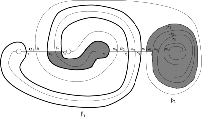
Figure 2. Domain belonging to $\phi$ and $i=3$.

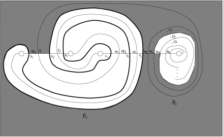
Figure 3. Domain belonging to $\psi$ and $i=3$.

    

Proof of Proposition 3.2. Consider the equivalence class containing the elements $\{x_{1},w_{9}\}$, $\{x_{2},w_{8}\}$, and $\{x_{3},w_{7}\}$, denoted $a$, $b$, and $c$ respectively. Let $\mathfrak{s}_{0}$ denote the ${\mathrm{Spin}}^{c}$ structure corresponding to this equivalence class and the basepoint $z_{5}$. According to Lemma 3.4, in this ${\mathrm{Spin}}^{c}$ structure we have

$$\partial^{\infty}[a,j]=\pm[b,j-1],\ \ \ \partial^{\infty}[c,j]=\pm[b,j-1].$$

From the fact that $(\partial^{\infty})^{2}=0$, it follows that $\partial^{\infty}[b,j]=0$. The calculations for $\mathfrak{s}_{0}$ follow.

Varying the basepoint $z_{r}$ with $r=6,...,k-2$, we capture all the other ${\mathrm{Spin}}^{c}$ structures. According to Lemma 3.4, with this choice,

$$\partial^{\infty}[a,j]=\pm[b,j],\ \ \ \partial^{\infty}[c,j]=\pm[b,j-1]$$

This implies the result for all the other ${\mathrm{Spin}}^{c}$ structures. ∎

More generally let $Y_{m,n}$ denote the oriented 3-manifold obtained by a $+n$ surgery along the torus knot $T_{2,2m+1}$. (Again we use the left-handed versions of these knots, so for example $+1$ surgery would give the Brieskorn sphere $\Sigma(2,2m+1,4m+3)$). In the following we will compute the Floer homologies of $Y_{m,n}$ for the case $n>6m$.

First note that $Y_{m,n}$ admits a Heegaard decomposition of genus 2. The corresponding picture is analogous to the $m=1$ case, except that now $\beta_{1}$ and $\beta_{2}$ spiral more around $\alpha_{1}$, $\alpha_{2}$, see Figure 4 for $m=2$. In general the $\beta_{1}$ curve hits both $\alpha_{1}$ and $\alpha_{2}$ in $2m+1$ points, $\beta_{2}$ intersects $\alpha_{1}$ in $2m$ points and $\alpha_{2}$ in $n+6m$ points. Let $x_{1},...,x_{2m+1}$ denote the intersection points of $\alpha_{1}\cap\beta_{1}$, labeled from left to right. Similarly let $w_{1},...,w_{n+6m}$ denote the intersection points of $\alpha_{2}\cap\beta_{2}$ labeled from left to right. We also choose basepoints $z_{1},z_{2},...,z_{n+4m}$ in the spiral at the right hand side, labeled from outside to inside.

Figure 4. $+n$ surgery on the $(2,5)$ torus knot.

Lemma 3.5.

If $n>6m$, then there is an equivalence class containing only the intersection points $a_{i}=\{x_{i},w_{8m+2-i}\}$ for $i=1,...,2m+1$. Furthermore if $\mathfrak{s}_{t}$ denotes the ${\mathrm{Spin}}^{c}$ structure determined by this equivalence class and base point $z_{5m+t}$, for $1-m\leq t\leq n-m$, then in this ${\mathrm{Spin}}^{c}$ structure we have

• $\partial_{\infty}[a_{2v+1},j]=\pm[a_{2v},j]\pm[a_{2v+2},j-1]$, for $t<m-2v$

• $\partial_{\infty}[a_{2v+1},j]=\pm[a_{2v},j]\pm[a_{2v+2},j]$ for $t=m-2v$,

• $\partial_{\infty}[a_{2v+1},j]=\pm[a_{2v},j-1]\pm[a_{2v+2},j],$ for $t>m-2v$,

where $0\leq v\leq m$, and $a_{0}=a_{2m+2}=0$.

Proof. This is the same argument as in the $m=1$ case, together with the observation that if $\phi\in\pi_{2}(a_{2v+1},a_{2\ell})$, and $\ell\neq v$ or $v+1$, and $\mu(\phi)=1$, then the domain ${\mathcal{D}}(\phi)$ contains regions with negative coefficients (so the moduli space is empty). Moreover, since $(\partial^{\infty})^{2}=0$, it follows that $\partial^{\infty}([a_{2v},i])=0$.         

Note that $\mathfrak{s}_{t+1}-\mathfrak{s}_{t}\in H^{2}(Y_{m,n})$ is the Poincare dual of the meridian of the knot. Since the meridian of the knot generates $H_{1}(Y_{m,n})=\mathbb{Z}/n\mathbb{Z}$, it follows that $\{\mathfrak{s}_{t}|\ 1-m\leq t\leq n-m\}={\mathrm{Spin}}^{c}(Y_{m,n})$, i.e we get all the ${\mathrm{Spin}}^{c}$ structures this way. Now a straightforward computation gives the Floer homology groups of $Y_{m,n}$:

Corollary 3.6.

Let $Y=Y_{m,n}$ denote the three-manifold obtained by $+n$ surgery on the $(2,2m+1)$ torus knot. Suppose that $n>6m$, and let $\mathfrak{s}_{t}$ denote the ${\mathrm{Spin}}^{c}$ structures defined above. For $m-1<t\leq n-m$ the Floer theories are trivial, i.e $\widehat{HF}(Y_{m,n},\mathfrak{s}_{t})\cong\mathbb{Z}$, $HF_{\rm red}(Y_{m,n},\mathfrak{s}_{t})=0$, $HF^{+}(Y_{m,n},\mathfrak{s}_{t})\cong{\mathcal{T}}^{+}$, and $HF^{-}(Y_{m,n},\mathfrak{s}_{t})\cong{\mathcal{T}}^{-}$. For $-m+1\leq t<0$, the Floer homologies of $\mathfrak{s}_{t}$ are isomorphic to the corresponding Floer homologies of $\mathfrak{s}_{-t}$. Furthermore for $0\leq t\leq m-1$ we have

1. $\widehat{HF}(Y_{m,n},\mathfrak{s}_{t})$ is generated by $a,b,c$ with $\mathrm{gr}(b,a)=1+2v_{m,t}+2t$, $\mathrm{gr}(b,c)=1+2v_{m,t}$.

2. $HF^{+}(Y_{m,n},\mathfrak{s}_{t})$ is generated by $x_{i}$, $y_{j}$, for $0\leq i$, $0\leq j\leq v_{m,t}$, $\mathrm{gr}(y_{j},x_{i})=2(j-i+t)$ and $U_{+}(x_{i})=x_{i-1}$, $U_{+}(x_{0})=0$, $U_{+}(y_{i})=y_{i-1}$, $U_{+}(y_{0})=0$.

3. $HF^{-}(Y_{m,n},\mathfrak{s}_{t})$ is generated by $x_{i}$, $y_{j}$, for $i<0$, $0\leq j\leq v_{m,t}$, $\mathrm{gr}(y_{j},x_{i})=2(j-i+t)-1$ and $U_{-}(x_{i})=x_{i-1}$, $U_{-}(y_{i})=y_{i-1}$, $U_{-}(y_{0})=0$.

4. $HF_{\rm red}(Y_{m,n},\mathfrak{s}_{t})$ is generated by $y_{j}$, for $0\leq j\leq v_{m,t}$, $\mathrm{gr}(y_{i},y_{j})=2i-2j$,

where $v_{m,t}=\lfloor\frac{m-t-1}{2}\rfloor$, i.e. the greatest integer less than or equal to $(m-t-1)/2$.

Remark 3.7.

The symmetry of the Floer homology under the involution on the set of ${\mathrm{Spin}}^{c}$ structures ensures that $\mathfrak{s}_{0}$ comes from a spin structure. If $n$ is odd, there is a unique spin structure. With some additional work one can show that, regardless of the parity of $n$, $\mathfrak{s}_{0}$ can be uniquely characterized as follows. Let $X_{m,n}$ be the four-manifold obtained by adding a two-handle to the four-ball along the $(2,2m+1)$ torus knot with framing $+n$. Then, $\mathfrak{s}_{0}$ extends to give a ${\mathrm{Spin}}^{c}$ structure ${\mathfrak{r}}$ over $X_{m,n}$ with the property that $\langle c_{1}({\mathfrak{r}}),[S]\rangle=\pm n$, where $S$ is a generator of $H_{2}(X_{m,n};\mathbb{Z})$. This calculation, which is done in [30], follows easily from the four-dimensional theory developed in [31].

In fact, Lemma 3.5 can be used to prove that for any ${\mathrm{Spin}}^{c}$ structure on $Y_{m,n}$, $HF^{\infty}(Y_{m,n},\mathfrak{s})\cong{\mathcal{T}}^{\infty}$. Actually, it will be shown in Section 10 that for any rational homology three-sphere, $HF^{\infty}(Y,\mathfrak{s})\cong{\mathcal{T}}^{\infty}$.

4. Comparison with Seiberg-Witten theory

4.1. Equivariant Seiberg-Witten Floer homology

We recall briefly the construction of equivariant Seiberg-Witten Floer homologies $HF_{{\rm to}}^{SW}$, $HF_{{\rm from}}^{SW}$ and $HF^{SW}_{{\rm red}}$. Our presentation here follows the lectures of Kronheimer and Mrowka [16]. For more discussion, see [3] for the instanton Floer homology analogue, and also [11], [21], [38].

Let $Y$ be an oriented rational homology 3-sphere, and $\mathfrak{s}\in{\mathrm{Spin}}^{c}(Y)$. After fixing additional data (a Riemannian metric over $Y$ and some perturbation) the Seiberg-Witten equations over $Y$ in the ${\mathrm{Spin}}^{c}$ structure $\mathfrak{s}$ give a smooth moduli space consisting of finitely many irreducible solutions $\gamma_{1},...,\gamma_{k}$ and a smooth reducible solution $\theta$.

The chain-group $CF_{{\rm to}}^{SW}$ is freely generated by $\gamma_{1},...,\gamma_{k}$ and $[\theta,i]$, for $i\geq 0$. Let $S$ denote this set of generators. The relative grading is given by

$$\mathrm{gr}(\gamma_{j},[\theta,i])={\rm dim}\left(\mathcal{M}(\gamma_{j},\theta)\right)-2i,\ \ \mathrm{gr}(\gamma_{j},\gamma_{i})={\rm dim}\left(\mathcal{M}(\gamma_{j},\gamma_{i})\right)$$

where $\mathcal{M}(\gamma_{j},\theta)$ (resp. $\mathcal{M}(\gamma_{j},\gamma_{i})$) denotes the Seiberg-Witten moduli space of flows from $\gamma_{j}$ to $\theta$ (resp. $\gamma_{j}$ to $\gamma_{i}$).

Definition 4.1.

For each $x,y\in S$ with $\mathrm{gr}(x,y)=1$ we define an incidence number $c(x,y)\in\mathbb{Z}$, in the following way:

1. If $x=[\theta,i]$, then $c(x,y)=0$,

2. $c(\gamma_{j},\gamma_{i})=\#{\widehat{\mathcal{M}}}(\gamma_{j},\gamma_{i})$,

3. $c(\gamma_{j},[\theta,0])=\#{\widehat{\mathcal{M}}}(\gamma_{j},\theta)$

4. $c(\gamma_{j},[\theta,i])=\#({\widehat{\mathcal{M}}}(\gamma_{j},\theta)\cap\mu({\rm pt})^{i})$,

where ${\widehat{\mathcal{M}}}$ denotes the quotient of $\mathcal{M}$ by the $\mathbb{R}$ action of translations, and $\cap\mu({\rm pt})^{i}$ denotes cutting down by a geometric representative for $\mu({\rm pt})^{i}$ in a time-slice close to $\theta$ (measured using the Chern-Simons-Dirac functional). We define the boundary map $\partial_{\rm to}$ on $CF_{{\rm to}}^{SW}$ by

$$\partial_{\rm to}(x)=\sum_{\{y\in S|\ \mathrm{gr}(x,y)=1\}}c(x,y)\cdot y$$

It follows from the broken flowline compactification of two-dimensional flows, modulo the $\mathbb{R}$ action, that $(CF_{{\rm to}}^{SW},\partial_{\rm to})$ is a chain complex. Let $HF_{{\rm to}}^{SW}$ denote the corresponding relative $\mathbb{Z}$ graded homology.

Similarly we can define the chain complex $(CF_{{\rm from}}^{SW},\partial_{\rm from})$. $CF_{{\rm from}}^{SW}$ is freely generated by $\gamma_{1},...,\gamma_{k}$ and $[\theta,i]$, for $i\leq 0$. Let $S^{\prime}$ denote this set of generators. The relative grading is determined by

$$\mathrm{gr}([\theta,i],\gamma_{j})={\rm dim}\left(\mathcal{M}(\theta,\gamma_{j})\right)+2i,\ \ \mathrm{gr}(\gamma_{j},\gamma_{i})={\rm dim}\left(\mathcal{M}(\gamma_{j},\gamma_{i})\right).$$

Definition 4.2.

For each $x,y\in S^{\prime}$ with $\mathrm{gr}(x,y)=1$ we define an incidence number $c^{\prime}(x,y)\in\mathbb{Z}$, in the following way:

1. If $y=[\theta,i]$, then $c^{\prime}(x,y)=0$,

2. $c^{\prime}(\gamma_{j},\gamma_{i})=\#{\widehat{\mathcal{M}}}(\gamma_{j},\gamma_{i})$,

3. $c^{\prime}([\theta,0],\gamma_{j})=\#{\widehat{\mathcal{M}}}(\theta,\gamma_{j})$

4. If $i<0$, then $c^{\prime}([\theta,i],\gamma_{j})=\#({\widehat{\mathcal{M}}}(\theta,\gamma_{j})\cap\mu({\rm pt})^{-i})$.

We define the boundary map $\partial_{\rm from}$ on $CF_{{\rm from}}^{SW}$ by

$$\partial_{\rm from}(x)=\sum_{\{y\in S^{\prime}|\ \mathrm{gr}(x,y)=1\}}c^{\prime}(x,y)\cdot y.$$

Again this gives a chain complex and we denote its homology by $HF_{{\rm from}}^{SW}$. We also have a chain map

$$f:CF_{{\rm to}}^{SW}\longrightarrow CF_{{\rm from}}^{SW}$$

given by $f(\gamma_{j})=\gamma_{j}$, $f([\theta,i])=0$. Let $f_{*}$ denote the induced map between the Floer-homologies, and define

$$HF^{SW}_{{\rm red}}=HF_{{\rm to}}^{SW}/({\rm Ker}f_{*}).$$

One reason to introduce these equivariant Floer-homologies is that the irreducible Seiberg-Witten Floer homology (generated only by $\gamma_{1},...,\gamma_{k}$) is metric dependent. Analogy with equivariant Morse theory suggests that the equivariant theories are metric independent. Indeed the following was stated by Kronheimer and Mrowka, [16].

Conjecture 4.3.

For oriented rational homology $3$-spheres $Y$ and ${\mathrm{Spin}}^{c}$ structures $\mathfrak{s}\in{\mathrm{Spin}}^{c}(Y)$ the equivariant Seiberg-Witten Floer homologies $HF_{{\rm to}}^{SW}(Y,\mathfrak{s})$, $HF_{{\rm from}}^{SW}(Y,\mathfrak{s})$, and $HF^{SW}_{{\rm red}}(Y,\mathfrak{s})$ are well-defined, i.e. they are independent of the particular choice of metrics and perturbations.

4.2. Computations

In this subsection we will compute $HF_{{\rm to}}^{SW}$, $HF_{{\rm from}}^{SW}$ and $HF^{SW}_{{\rm red}}$ for the 3-manifolds studied in Section 3, and for a particular choice of perturbations of the Seiberg-Witten equations. First, note that lens spaces all have trivial Seiberg-Witten Floer homology, since they admit metrics with positive scalar curvature, in particular, $HF_{{\rm to}}^{SW}(L(p,q),\mathfrak{s})$, $HF_{{\rm from}}^{SW}(L(p,q),\mathfrak{s})$ and $HF^{SW}_{{\rm red}}(L(p,q),\mathfrak{s})$ are isomorphic to ${\mathcal{T}}^{+}$, ${\mathcal{T}}^{-}$, and $0$ respectively. Note that all the 3-manifolds $Y=Y_{m,n}$ from Section 3 are Seifert-fibered so we can use [25] to compute their Seiberg-Witten Floer homology.

Proposition 4.4.

Let $Y=Y_{m,n}$ denote the oriented $3$-manifold obtained by $+n$ surgery along the torus knot $T_{2,2m+1}$. Suppose also that $n>6m$. Then for each $\mathfrak{s}\in{\mathrm{Spin}}^{c}(Y)$ we have

$$HF_{{\rm to}}^{SW}(Y,\mathfrak{s})\cong HF^{+}(Y,\mathfrak{s}),\ \ \ HF_{{\rm from}}^{SW}(Y,\mathfrak{s})\cong HF^{-}(Y,\mathfrak{s}),\ \ \ HF^{SW}_{{\rm red}}(Y,\mathfrak{s})\cong HF_{\rm red}(Y,\mathfrak{s}),$$

where the isomorphisms are between relative $\mathbb{Z}$-graded Abelian groups, and $HF_{{\rm to}}^{SW}(Y,\mathfrak{s})$, $HF_{{\rm from}}^{SW}(Y,\mathfrak{s})$, $HF^{SW}_{{\rm red}}(Y,\mathfrak{s})$ are computed using a reducible connection on the tangent bundle induced from the Seifert fibration of $Y$, and an additional perturbation.

Proof. First note that $Y_{m,n}$ is the boundary of the 4-manifold described by the plumbing diagram in Figure 5, where the number of $-2$ spheres in the right chain is $n+4m+1$. This gives a description of $Y_{m,n}$ as the total space of an orbifold circle bundle over the sphere with $3$ marked points with multiplicities $2,2m+1,k$ respectively, where $k=n+4m+2$. The circle bundle $N$ has Seifert data

$$N=(-2,1,m+1,k-1).$$

and the canonical bundle is $K=(-2,1,2m,k-1)$.

Figure 5.

Now we can apply [25] to compute the irreducible solutions, relative gradings and the boundary maps.

Let us recall that for the unperturbed moduli space there is a 2 to 1 map from the set of irreducible solutions to the set of orbifold divisors $E$ with $E\geq 0$ and

$${\rm deg}E<{{\rm deg}(K)\over 2},$$

where the preimage consists of a holomorphic and an anti-holomorphic solution, that we denote by ${\mathcal{C}}^{+}(E)$ and ${\mathcal{C}}^{-}(E)$ respectively. Note that ${\mathcal{C}}^{+}(E)$, ${\mathcal{C}}^{-}(E)$ lie in the ${\mathrm{Spin}}^{c}$ structures determined by the line-bundles $E$, $K\otimes E^{-1}$ respectively.

In order to simplify the computation we will use a certain perturbation of the Seiberg-Witten equation. Using the notation of [26] this perturbation depends on a real parameter $u$, and corresponds to adding a two-form $iu(*d\eta)$ to the curvature equation, where $\eta$ is the connection form for $Y$ over the orbifold. Now holomorphic solutions ${\mathcal{C}}^{+}(E)$ correspond to effective divisors with

$${\rm deg}E<{{\rm deg}(K)\over 2}-u{{\rm deg}(N)\over 2},$$

and anti-holomorphic solutions ${\mathcal{C}}^{-}(E)$ correspond to effective divisors with

$${\rm deg}E<{{\rm deg}(K)\over 2}+u{{\rm deg}(N)\over 2}.$$

According to [18] the expected dimension of the moduli space between the reducible solution $\theta$ and ${\mathcal{C}}^{\pm}(E)$ is computed by

$${\rm dim}\mathcal{M}(\theta,{\mathcal{C}}^{\pm}(E))=1+2\left(\sum_{i\in I^{\pm}}\chi(E\otimes N^{i})\right),$$

where $\chi(E\otimes N^{i})$ denotes the holomorphic Euler characteristic of the bundle $E\otimes N^{i}$, and $I^{\pm}\subset\mathbb{Z}$ is given by the inequalities

$${\rm deg}E<{\rm deg}(E\otimes N^{i})<{{\rm deg}(K)\over 2}\mp u{{\rm deg}(N)\over 2}.$$

Returning to our examples let $E(a,b)$ denote the divisor $(0,0,a,b)$. It is easy to see that ${\mathcal{C}}^{-}(E(a,b))$ and ${\mathcal{C}}^{-}(E(a+1,b-2))$ are in the same ${\mathrm{Spin}}^{c}$ structure. Also ${\mathcal{C}}^{-}(E(0,b))$ and ${\mathcal{C}}^{+}(E(0,2m-2-b))$ are in the same ${\mathrm{Spin}}^{c}$ structure. From now on let $\mathfrak{s}_{0}$ denote the ${\mathrm{Spin}}^{c}$ structure given by the line bundle $E(0,m-1)$, and $\mathfrak{s}_{t}$ corresponds to the line-bundle $E(0,m-1+t)$. Clearly $\mathfrak{s}_{t}\equiv\mathfrak{s}_{t+n}$, since $H_{1}(Y,\mathbb{Z})=\mathbb{Z}/n\mathbb{Z}$.

Since

$${\rm deg}E(a,b)={a\over{2m+1}}+{b\over k},\ \ \ {\rm deg}K={2m-1\over 4m+2}-{1\over k},$$

for all $\mathfrak{s}_{t}$ with $n/4\leq|t|\leq n/2$ the unperturbed moduli space (with $u=0$) have no irreducible solutions. It follows that $HF_{{\rm to}}^{SW}(Y,\mathfrak{s}_{t})$ and $HF_{{\rm from}}^{SW}(Y,\mathfrak{s}_{t})$ are generated by $[\theta,i]$ and we have the corresponding isomorphisms with ${\mathcal{T}}^{+}$, ${\mathcal{T}}^{-}$ respectively.

Clearly the $J$ action maps $\mathfrak{s}_{t}$ to $\mathfrak{s}_{-t}$, so in the light of the $J$ symmetry in Seiberg-Witten theory, it is enough to compute the equivariant Floer homologies for $0\leq t\leq n/4$. For these ${\mathrm{Spin}}^{c}$ structures let us fix a perturbation with parameter $u$ satisfying

$${\rm deg}(K)-u{\rm deg}(N)=-\epsilon,$$

where $\epsilon>0$ is sufficiently small. This perturbation eliminates all the holomorphic solutions. It still remains to compute the anti-holomorphic solutions.

First let $0\leq t\leq m-1$. Since

$${\rm deg}E(a,b)={a\over{2m+1}}+{b\over k},\ \ \ {\rm deg}K={2m-1\over 4m+2}-{1\over k},$$

the irreducible solutions in $\mathfrak{s}_{t}$ are $\delta_{r}={\mathcal{C}}^{-}(E(r,m-1-t-2r))$ for $0\leq r\leq{m-1-t\over 2}$. It is easy to see from [25], see also [26], that the irreducible solutions and $\theta$ are all transversally cut out by the equations.

Computing the holomorphic Euler characteristic we get $\chi(E\otimes N^{2i})=1,$ for $0<2i\leq m-1-t-2r$, $\chi(E\otimes N^{2i+1})=-1,$ for $m-1-t-2r<2i+1\leq 2(m-r)-1$, and $\chi(E\otimes N^{j})=0$ for all other $j\in I^{-}$, where $E=E(r,m-1-t-2r)$. The dimension formula then gives

$${\rm dim}\mathcal{M}(\theta,\delta_{r})=-2t-2r-1.$$

As a corollary we see that $\partial_{\rm from}$ is zero, since all these moduli spaces have negative formal dimensions, and relative gradings between the irreducible generators are even. In $CF_{{\rm to}}^{SW}$ the relative gradings between all the generators are even, so $\partial_{\rm to}$ is trivial as well. Now the isomorphism between $HF_{{\rm to}}^{SW}(Y,\mathfrak{s}_{t})$ and $HF^{+}(Y,\mathfrak{s}_{t})$ corresponds to mapping $[\theta,i]$ to $x_{i}$, and $\delta_{r}$ to $y_{r}$. Similarly the isomorphism between $HF_{{\rm from}}^{SW}(Y,\mathfrak{s}_{t})$ and $HF^{-}(Y,\mathfrak{s}_{t})$ corresponds to mapping $[\theta,i]$ to $x_{i-1}$, and $\delta_{r}$ to $y_{r}$. Furthermore $HF^{SW}_{{\rm red}}$ is freely generated by $\delta_{r}$ and the map $\delta_{r}\rightarrow y_{r}$ gives the isomorphism with $HF_{\rm red}$.

Now suppose that $m-1<t\leq n/4$. Then there are no irreducible solutions for the perturbed equation. So $HF_{{\rm to}}^{SW}$ and $HF_{{\rm from}}^{SW}$ are generated by $[\theta,i]$ and we have the corresponding isomorphisms with ${\mathcal{T}}^{+}$, ${\mathcal{T}}^{-}$ respectively.

For $-n/4\leq t<0$ we get the analogous results by replacing $u$ with $-u$.         

5. Euler characteristics

In this section, we analyze the Euler characteristics of the Floer homology theories. In Subsection 5.1, we show that the Euler characteristic of $\widehat{HF}$ is determined by $H_{1}(Y;\mathbb{Z})$. After that, we turn to the study of $HF^{+}$ for three-manifolds with $b_{1}>0$.

In [36], Turaev defines a torsion function

$$\tau_{Y}\colon{\mathrm{Spin}}^{c}(Y)\longrightarrow\mathbb{Z},$$

which is a generalization of the Alexander polynomial. This function can be calculated from a Heegaard diagram of $Y$ as follows. Fix integers $i$ and $j$ between $1$ and $g$, and consider corresponding tori

$${\mathbb{T}}_{\alpha}^{i}=\alpha_{1}\times..\times{\widehat{\alpha_{i}}}\times...\times\alpha_{g} {\mathbb{T}}_{\beta}^{j}=\beta_{1}\times..\times{\widehat{\beta_{j}}}\times...\times\beta_{g}$$ and

in $\mathrm{Sym}^{g-1}(\Sigma)$ (where the hat denotes an omitted entry). There is a map $\sigma$ from ${\mathbb{T}}_{\alpha}^{i}\cap{\mathbb{T}}_{\beta}^{j}$ to ${\mathrm{Spin}}^{c}(Y)$, which is given by thinking of each intersection point as a $(g-1)$-tuple of connecting trajectories from index one to index two critical points. Moreover, orienting $\alpha_{i}$, there is a distinguished trajectory connecting the index zero critical point to the index one critical point $a_{i}$ corresponding to $\alpha_{i}$; similarly, orienting $\beta_{j}$, there is a distinguished trajectory connecting the critical point $b_{j}$ corresponding to the circle $\beta_{j}$ to the index index three critical point in $Y$. This $(g+1)$-tuple of trajectories then gives rise to a ${\mathrm{Spin}}^{c}$ structure in the usual manner (modifying the upward gradient flow in the neighborhoods of these trajectories). Thus, we can define

$$\Delta_{i,j}(\mathfrak{s})=\pm\sum_{\{\mathbf{x}\in{\mathbb{T}}_{\alpha}^{i}\cap{\mathbb{T}}_{\beta}^{j}\big{|}\sigma(\mathbf{x})=\mathfrak{s}\}}\epsilon(\mathbf{x}),$$

where $\epsilon(\mathbf{x})$ is the local intersection number of ${\mathbb{T}}_{\alpha}^{i}$ and ${\mathbb{T}}_{\beta}^{j}$ at $\mathbf{x}$, and the overall sign depends on $i$, $j$ and $g$. (It is straightforward to verify that this geometric interpretation is equivalent to the more algebraic definition of $\Delta_{i,j}$ given in [36], see for instance Section LABEL:Theta:sec:Alex from [29].)

Choose $i$ and $j$ so that both $\alpha_{i}^{*}$ and $\beta_{j}^{*}$ have non-zero image in $H^{2}(Y;\mathbb{R})$. When $b_{1}(Y)>1$, Turaev’s torsion is characterized by the equation

(1) $$\tau(\mathfrak{s})-\tau(\mathfrak{s}+\alpha_{i}^{*})-\tau(\mathfrak{s}+\beta_{j}^{*})+\tau(\mathfrak{s}+\alpha_{i}^{*}+\beta_{j}^{*})=\Delta_{i,j}(\mathfrak{s}),$$

and the property that it has finite support. (To define $\beta_{j}^{*}$ here, let $C$ be a curve in $\Sigma$ with $\beta_{i}\cap C=\delta_{i,j}$, and let $\beta_{j}^{*}$ be Poincaré dual to the induced homology class in $Y$.) When $b_{1}(Y)=1$, we need a direction $t$ in $H^{2}(Y;\mathbb{R})$, which we think of as a component of $H^{2}(Y;\mathbb{R})-0$. Then, $\tau_{t}$ is characterized by the above equation and the property that $\tau_{t}$ has finite support amongst ${\mathrm{Spin}}^{c}$ structures whose first Chern class lies in the component of $t$.

For a three-manifold $Y$ with ${\mathrm{Spin}}^{c}$ structure $\mathfrak{s}$, the chain complex $CF^{+}(Y,\mathfrak{s})$ can be viewed as a relatively $\mathbb{Z}/{2}\mathbb{Z}$-graded complex (since the grading indeterminacy $\mathfrak{d}(\mathfrak{s})$ is always even). Alternatively, this relative $\mathbb{Z}/{2}\mathbb{Z}$ grading between $[\mathbf{x},i]$ and $[\mathbf{y},j]$ is calculated by orienting ${\mathbb{T}}_{\alpha}$ and ${\mathbb{T}}_{\beta}$, and letting the relative degree be given by the product of the local intersection numbers of ${\mathbb{T}}_{\alpha}$ and ${\mathbb{T}}_{\beta}$ at $\mathbf{x}$ and $\mathbf{y}$. This relative $\mathbb{Z}/{2}\mathbb{Z}$-grading can be used to define an Euler characteristic $\chi(HF^{+}(Y,\mathfrak{s}))$ (when the homology groups are finitely generated), which is well-defined up to an overall sign.

In this section, we relate the Euler characteristics of $HF^{+}(Y,\mathfrak{s})$ with Turaev’s torsion function, when $c_{1}(\mathfrak{s})$ is non-torsion. (The case where $c_{1}(\mathfrak{s})$ is torsion will be covered in Subsection 10.6, after more is known about $HF^{\infty}$; related results also hold for $HF^{-}$, c.f. Subsection 10.5.)

The overall sign on $\chi(HF^{+}(Y,\mathfrak{s}))$ will be pinned down once we define an absolute $\mathbb{Z}/{2}\mathbb{Z}$ grading on $HF^{+}(Y,\mathfrak{s})$ in Subsection 10.4.

5.1. Euler characteristic of $\widehat{HF}$

We first dispense with this simple object.

Proposition 5.1.

The Euler characteristic of $\widehat{HF}$ is given by

$$\chi(\widehat{HF}(Y,\mathfrak{s}))=\left\{\begin{array}[]{ll}1&{\text{if $b_{1}(Y)=0$}}\\ 0&{\text{if $b_{1}(Y)>0$}}\end{array}\right..$$

Proof. Both cases follow from the observation that $\chi(\widehat{HF}(Y,\mathfrak{s}))$ is independent of the ${\mathrm{Spin}}^{c}$ structure $\mathfrak{s}$. To see this, note that for any $\beta_{j}$, we can wind normal to the $\alpha$ so that $(\Sigma,\mbox{\boldmath$\alpha$},\mbox{\boldmath$\beta$},z)$ and $(\Sigma,\mbox{\boldmath$\alpha$},\mbox{\boldmath$\beta$},z^{\prime})$ are both weakly $\mathfrak{s}$-admissible, where $z$ and $z^{\prime}$ are two choices of basepoint which can be connected by an arc which meets only $\beta_{j}$. Now, both $\widehat{HF}(Y,\mathfrak{s})$ and $\widehat{HF}(Y,\mathfrak{s}+\mathrm{PD}[\beta_{j}^{*}])$ are calculated by the same equivalence class of intersection points, using the basepoint $z$ in the first case and $z^{\prime}$ in the second. This changes only the boundary map, but leaves the (finitely generated) chain groups unchanged, hence leaving the Euler characteristic unchanged.

The result for $b_{1}(Y)>0$ then follows from this observation, together with Theorem 2.3.

For the case where $b_{1}(Y)=0$, recall that the Heegaard decomposition gives $Y$ a chain complex with $g$ one-dimensional generators corresponding to the $\alpha$ (each of which is a cycle), and $g$ two-dimensional generators corresponding to the $\beta$. On the one hand, the determinant of the boundary map is the order of the finite group $H_{1}(Y;\mathbb{Z})$ (which, in turn, is the number of distinct ${\mathrm{Spin}}^{c}$ structures over $Y$); on the other hand, this determinant is easily seen to agree with the intersection number $\#({\mathbb{T}}_{\alpha}\cap{\mathbb{T}}_{\beta})=\sum_{\mathfrak{s}\in{\mathrm{Spin}}^{c}(Y)}\chi(\widehat{HF}(Y,\mathfrak{s}))$. The result follows from this, together with $\mathfrak{s}$-independence of $\chi(\widehat{HF}(Y,\mathfrak{s}))$.         

5.2. $\chi(HF^{+}(Y,\mathfrak{s}))$ when $b_{1}(Y)=1$ and $\mathfrak{s}$ is non-torsion

Our aim is to prove the following:

Theorem 5.2.

Suppose $b_{1}(Y)=1$. If $\mathfrak{s}$ is a non-torsion ${\mathrm{Spin}}^{c}$ structure, then $HF^{+}(Y,\mathfrak{s})$ is finitely generated, and indeed,

$$\chi(HF^{+}(Y,\mathfrak{s}))=\pm\tau_{t}(Y,\mathfrak{s}),$$

where $\tau_{t}$ is Turaev’s torsion function, with respect to the component $t$ of $H^{2}(Y;\mathbb{R})-0$ containing $c_{1}(\mathfrak{s})$.

As usual, the Euler characteristic appearing above can be thought of as the Euler characteristic of $HF^{+}(Y,\mathfrak{s})$ as a $\mathbb{Z}$-module; or, alternatively, we could consider $HF^{+}(Y,\mathfrak{s},\mathbb{F})$ with coefficients in an arbitrary field $\mathbb{F}$.

The proof of Theorem 5.2 occupies the rest of the present subsection.

Let $\mathfrak{s}$ be a non-torsion ${\mathrm{Spin}}^{c}$ structure on $Y$. Let $H$ be the generator of $H_{2}(Y;\mathbb{Z})$ with the property that

$$\langle c_{1}(\mathfrak{s}),H\rangle<0.$$

After handleslides, we can arrange that the periodic domain $\mathcal{P}$ corresponding to $H$ contains $\alpha_{1}$ with multiplicity one in its boundary.

Choose a curve $\gamma$ transverse to $\alpha_{1}$ and disjoint from all other $\alpha_{i}$ for $i>1$, oriented so that $\alpha_{1}\cap\gamma=+1$. (Note that $\mathrm{PD}[\gamma]=\alpha_{1}^{*}$.) This curve has the property, then, that

$$\langle PD[\gamma],H\rangle=-1.$$

Let ${\mathbb{T}}_{\gamma}=\gamma\times\alpha_{2}\times...\times\alpha_{g}$. Winding $\alpha_{1}$ $n$ times along $\gamma$, we obtain a new $\alpha$-torus, which we denote ${\mathbb{T}}_{\alpha}(n)$. For each intersection point $\mathbf{x}\in{\mathbb{T}}_{\gamma}\cap{\mathbb{T}}_{\beta}$ we obtain $2n$ intersection points in ${\mathbb{T}}_{\alpha}(n)\cap{\mathbb{T}}_{\beta}$

$$\mathbf{x}^{\pm}_{1},...,\mathbf{x}^{\pm}_{n},$$

which we order with decreasing distance to $\gamma$, with a sign $\pm$ indicating which side of $\gamma$ they lie on ($-$ indicates left, $+$ indicates right). We call the points in ${\mathbb{T}}_{\alpha}(n)\cap{\mathbb{T}}_{\beta}$ $\gamma$-induced: equivalently, a $\gamma$-induced intersection point between ${\mathbb{T}}_{\alpha}(n)$ and ${\mathbb{T}}_{\beta}$ is a $g$-tuple of points in $\Sigma$, one of which lies in the winding region about $\gamma$. It is easy to see that $\mathbf{x}^{+}_{i}$ and $\mathbf{x}^{-}_{i}$ lie in the same equivalence class: indeed, there is a canonical flow-line (with Maslov index $1$) connecting each $\mathbf{x}^{+}_{i}$ to $\mathbf{x}^{-}_{i}$. Thus, (for any choice of base-point $z$),

$$\mathfrak{s}_{z}(\mathbf{x}^{+}_{i})-\mathfrak{s}_{z}(\mathbf{x}^{+}_{j}) = (i-j)\mathrm{PD}(\gamma),$$

$$\mathfrak{s}_{z}(\mathbf{x}^{+}_{i}) = \mathfrak{s}_{z}(\mathbf{x}^{-}_{i}).$$

Figure 6. Winding transverse to $\alpha$. We have pictured, once again, the cylindrical neighborhood of $\gamma$, and an $\alpha$-curve obtained by winding six times transverse to $\gamma$. The basepoint $z$ is placed in the third region, and intersection points corresponding to some $\beta$ are labeled. The multiplicities correspond to the domain of a flow connecting $x_{5}^{+}$ to $x_{5}^{-}$.

Our twisting will always be done in a “sufficiently small” area, so that the area of each component of $\Sigma-{\mathrm{nd}}(\gamma)-\alpha_{1}-\alpha_{2}-...-\alpha_{g}-\beta_{1}-...-\beta_{g}$ is greater than $n$ times the area of ${\mathrm{nd}}(\gamma)$.

We will place our base-point $z$ to the right of $\gamma$, in the $\left(\frac{n}{2}\right)^{th}$ subregion of the winding region about $\gamma$. For this choice of basepoint, if $\mathbf{x}\in{\mathbb{T}}_{\gamma}\cap{\mathbb{T}}_{\beta}$ then the ${\mathrm{Spin}}^{c}$ structure induced by $\mathbf{x}^{\pm}_{n/2}$ is independent of $n$. Of course, the base-point is not uniquely determined by this requirement: this region is divided into components by the $\beta$-curves which intersect $\gamma$; but we fix any one such region, for the time being.

Lemma 5.3.

If we wind $n$ times, and place the basepoint in the $\left(\frac{n}{2}\right)^{th}$ subregion, and let $\mathcal{P}_{n}$ denote the corresponding periodic domain, then there is a constant $c$ with the property that we can find basepoints $w_{1}$ and $w_{2}$ (near $\gamma$ and away from $\gamma$ respectively), so that

$$n_{w_{1}}(\mathcal{P}_{n})\leq c-\frac{n}{2}, n_{w_{2}}(\mathcal{P}_{n})\geq c+\frac{n}{2}.$$ and

Lemma 5.4.

Fix a ${\mathrm{Spin}}^{c}$ structure $\mathfrak{s}\in Y$. Then, if $n$ is sufficiently large, the $\gamma$-induced intersection points of ${\mathbb{T}}_{\alpha}(n)\cap{\mathbb{T}}_{\beta}$ are the only ones which represent any of the ${\mathrm{Spin}}^{c}$ structures of the form $\mathfrak{s}+k\cdot\mathrm{PD}[\gamma]$ for $k\geq 0$.

Proof. The intersection points between ${\mathbb{T}}_{\alpha}(n)$ and ${\mathbb{T}}_{\beta}$ which are not induced from $\gamma$ correspond to the intersection points between the original ${\mathbb{T}}_{\alpha}$ and ${\mathbb{T}}_{\beta}$. So, suppose that $\mathbf{x}$ is an intersection point between ${\mathbb{T}}_{\alpha}$ and ${\mathbb{T}}_{\beta}$ (there are, of course, finitely many such intersection points), and let $z_{0}$ be some basepoint outside the winding region. As we wind $\alpha_{1}$ $n$ times, and place the new basepoint $z$ inside the winding region as above (so as not to cross any additional $\beta$-curves), we see that

$$s_{z}(\mathbf{x})-s_{z_{0}}(\mathbf{x})=-\frac{n}{2}\mathrm{PD}[\gamma],$$

where we think of $[\gamma]$ a one-dimension homology class in $Y$. The lemma then follows.         

Let $({\mathbb{T}}_{\alpha}(n)\cap{\mathbb{T}}_{\beta})^{L}\subset{\mathcal{S}}$ denote subset of $\gamma$-induced intersection points where the $\alpha_{1}$ part lies to the “left” of $\gamma$, and $({\mathbb{T}}_{\alpha}(n)\cap{\mathbb{T}}_{\beta})^{R}$ denote subset of $\gamma$-induced intersection points where the $\alpha_{1}$ part lies to the “right” of $\gamma$. (Note here that ${\mathcal{S}}$ denotes the subset of intersection points which induce the given ${\mathrm{Spin}}^{c}$ structure $\mathfrak{s}$ over $Y$.) There are corresponding subgroups $L^{+}$ and $R^{+}\subset CF^{+}(Y)$; similarly we have $L^{\infty}$ and $R^{\infty}\subset CF^{\infty}(Y)$.

Lemma 5.5.

Fix $\mathfrak{s}\in{\mathrm{Spin}}^{c}(Y)$ and an integer $n$ sufficiently large (in comparison with $\langle c_{1}(\mathfrak{s}),\mathcal{P}\rangle$). Then, for each $\gamma$-induced pair $\mathbf{x}^{+}$ and $\mathbf{y}^{-}$ inducing $\mathfrak{s}$, there are at most two homotopy classes $\phi^{\mathrm{in}},\phi^{\mathrm{out}}\in\pi_{2}(\mathbf{x}^{+},\mathbf{y}^{-})$ with Maslov index one and with only non-negative multiplicities. Moreover, there are no such classes in $\pi_{2}(\mathbf{y}^{-},\mathbf{x}^{+})$.

Proof. Assume $\mathrm{gr}(\mathbf{x}^{+},\mathbf{y}^{-})$ is odd, and let $\phi^{\mathrm{in}}_{n}$ be the class with $\mu(\phi^{\mathrm{in}}_{n})=1$, and whose $\alpha_{1}$ boundary lies entirely inside the tubular neighborhood of $\gamma$. We claim that ${\mathcal{D}}(\phi^{\mathrm{in}}_{n+2})$ is obtained from ${\mathcal{D}}(\phi^{\mathrm{in}}_{n})$ by winding only its $\alpha_{1}$-boundary (and hence leaving the domain unchanged outside the winding region). This follows from the fact that the Maslov index is unchanged under totally real isotopies of the boundary. It follows then that the multiplicities of $\phi^{\mathrm{in}}_{n}$ inside a neighborhood of $\gamma$ grow like $n/2$. Recall that the multiplicities of $\mathcal{P}_{n}$ inside grow like $-n/2$, while outside they grow like $n/2$.

Now, the set of all $\mu=1$ homotopic classes connecting $\mathbf{x}^{+}$ to $\mathbf{y}^{-}$ is given by

$$\phi^{\mathrm{in}}_{n}+k\left(\mathcal{P}_{n}-\frac{\langle c_{1}(\mathfrak{s}),\mathcal{P}\rangle}{2}S\right).$$

If this class is to have non-negative multiplicities, we must have that $k=0$ or $1$. This proves the assertion concerning classes from $\mathbf{x}^{+}$ to $\mathbf{y}^{-}$, letting $\phi^{\mathrm{out}}_{n}=\phi^{\mathrm{in}}_{n}+\left(\mathcal{P}_{n}-\frac{\langle c_{1}(\mathfrak{s}),\mathcal{P}\rangle}{2}S\right)$.

Considering classes from $\mathbf{y}^{-}$ to $\mathbf{x}^{+}$, note that all $\mu=1$ classes have the form

$$(S-\phi^{\mathrm{in}})+k\left(\mathcal{P}_{n}-\frac{\langle c_{1}(\mathfrak{s}),\mathcal{P}\rangle}{2}S\right).$$

When $k<0$, these classes have negative multiplicities outside $\gamma$. When $k\geq 0$, these have negative multiplicities inside the neighborhood of $\gamma$.         

Proposition 5.6.

Given a ${\mathrm{Spin}}^{c}$ structure $\mathfrak{s}$ and an $n$ sufficiently large, the subgroup $L^{\infty}\subset CF^{\infty}(Y,\mathfrak{s})$ is a subcomplex.

Proof. This follows immediately from the previous lemma.         

Of course, the above proposition allows us to think of $R^{\infty}$ as a chain complex, as well, with differential induced from the quotient structure $CF^{\infty}/L^{\infty}$.

There is a natural map

$$\delta\colon R^{\infty}\longrightarrow L^{\infty}$$

given by taking the $L^{\infty}$-component of the boundary of each element in $R^{\infty}$. This induces the connecting homomorphism for the long exact sequence associated to the short exact sequence of complexes:

$$\begin{CD}0@>{}>{}>L^{\infty}@>{}>{}>CF^{\infty}@>{}>{}>R^{\infty}@>{}>{}>0.\end{CD}$$

To understand the homomorphism $\delta$, let

$$f_{1}\colon R^{\infty}\longrightarrow L^{\infty}$$

be the homomorphism induced by $f_{1}([\mathbf{x}^{+}_{i},j])=[\mathbf{x}^{-}_{i},j-n_{z}(\phi)]$, where $\phi$ the disk connecting $\mathbf{x}^{+}_{i}$ to $\mathbf{x}^{-}_{i}$ which is supported in the tubular neighborhood of $\gamma$.

We can define an ordering on the $\gamma$-induced intersection points representing $\mathfrak{s}$ as follows. Let $[\mathbf{x},i],[\mathbf{y},j]\in{\mathfrak{S}}\times\mathbb{Z}$, then there is a unique $\phi\in\pi_{2}(\mathbf{x},\mathbf{y})$ with $n_{z}(\phi)=i-j$ and $\partial({\mathcal{D}}(\phi))\cap\alpha_{1}$ supported inside the tubular neighborhood of $\gamma$. We denote the class $\phi$ by $\phi_{[\mathbf{x},i],[\mathbf{y},j]}$. We then say that

$$[\mathbf{x},i]>[\mathbf{y},j]$$

if

$$\mu(\phi_{[\mathbf{x},i],[\mathbf{y},j]})>0$$

or if

$$\mu(\phi_{[\mathbf{x},i],[\mathbf{y},j]})=0$$

and the area $\mathcal{A}({\mathcal{D}}(\phi_{[\mathbf{x},i],[\mathbf{y},j]}))>0$. Note that an ordering gives us a partial ordering for elements in $CF^{\infty}(Y,\mathfrak{s})$: fix $\xi,\eta\in CF^{+}(Y,\mathfrak{s})$, we say that $\xi<\eta$ if each $[\mathbf{x},i]\in{\mathcal{S}}\times\mathbb{Z}$ which appears with non-zero multiplicity in the expansion of $\xi$ is smaller than each $[\mathbf{y},j]\in{\mathcal{S}}\times\mathbb{Z}$ which appears with non-zero multiplicity in the expansion of $\eta$.

In the following lemma, it is crucial to work with negative ${\mathrm{Spin}}^{c}$ structures, i.e. those for which $\langle c_{1}(\mathfrak{s}),\mathcal{P}\rangle<0$.

Lemma 5.7.

If $\mathfrak{s}$ is a negative ${\mathrm{Spin}}^{c}$ structure, then the map

$$\delta\colon R^{\infty}\longrightarrow L^{\infty}$$

can be written as

$$\delta=f_{1}+f_{2},$$

so that

$$f_{2}(g)<f_{1}(g)$$

for each $g=[\mathbf{x},i]\in R^{\infty}$.

Proof. Consider a pair of generators $[\mathbf{x}^{+},i]$ and $[\mathbf{y}^{-},j]$, for which the coefficient of $\delta$ is non-zero, i.e. that gives a homotopy class $\psi$ for which $\mu(\psi)=1$ and ${\mathcal{D}}(\psi)\geq 0$. Thus, by Lemma 5.5, there are two possible cases, where $\psi=\phi^{\mathrm{in}}$ or $\psi=\phi^{\mathrm{out}}$ (for $\mathbf{x}^{+}$ and $\mathbf{y}^{-}$). Note also that $\phi^{\mathrm{in}}=\phi_{[\mathbf{x}^{+},i][\mathbf{y}^{-},j]}$.

The case where $\psi=\phi^{\mathrm{in}}$, has two subcases, according to whether or not $[\mathbf{y}^{-},j]=f_{1}([\mathbf{x}^{+},i])$. If $[\mathbf{y}^{-},j]=f_{1}([\mathbf{x}^{+},i])$, $\psi=\phi_{[\mathbf{x}^{+},i]f_{1}([\mathbf{x}^{+},i])}$, and it follows easily that $\#\mathcal{M}(\psi)=1$. Since the periodic domains have both positive and negative coefficients, the $[\mathbf{y}^{-},j]$ coefficient of $f_{2}[\mathbf{x}^{+},i]$ must vanish. If $[\mathbf{y}^{-},j]\neq f_{1}([\mathbf{x}^{+},i])$, then the domain of $\phi_{f_{1}([\mathbf{x}^{+},i]),[\mathbf{y}^{-},j]}$ must include some region outside the neighborhood of $\gamma$. Moreover, since

$$\phi_{[\mathbf{x}^{+},i],f_{1}([\mathbf{x}^{+},i])}+\phi_{f_{1}([\mathbf{x}^{+},i]),[\mathbf{y}^{-},j]}=\psi,$$

we have that $\mu(\phi_{f_{1}([\mathbf{x}^{+},i]),[\mathbf{y}^{-},j]})=0$; but since the support of the twisting region is sufficiently small, it follows that

$$\mathcal{A}(\phi_{f_{1}([\mathbf{x}^{+},i]),[\mathbf{y}^{-},j]})>0;$$

i.e. $f_{1}([\mathbf{x}^{+},i])>[\mathbf{y}^{-},j]$.

When $\psi=\phi^{\mathrm{out}}$, it is easy to see that

$$\phi_{[\mathbf{x}^{+},i],[\mathbf{y}^{-},j]}=\phi^{\mathrm{out}}-\mathcal{P}.$$

It follows that $\mu(\phi_{[\mathbf{x}^{+},i],[\mathbf{y}^{-},j]})=1-\langle c_{1}(\mathfrak{s}),H(\mathcal{P})\rangle$. Moreover,

$$\phi_{[\mathbf{x}^{+},i],f_{1}([\mathbf{x}^{+},i])}+\phi_{f_{1}([\mathbf{x}^{+},i]),[\mathbf{y}^{-},j]}=\phi_{[x^{+},i],[\mathbf{y}^{-},j]},$$

so $\mu(\phi_{f_{1}([\mathbf{x}^{+},i]),[\mathbf{y}^{-},j]})=-\langle c_{1}(\mathfrak{s}),H(\mathcal{P})\rangle>0$, by our hypothesis on $\mathfrak{s}$, so that $f_{1}([\mathbf{x}^{+},i])>[\mathbf{y}^{-},j]$.         

Proposition 5.8.

For negative ${\mathrm{Spin}}^{c}$ structures $\mathfrak{s}$, the map $\delta^{+}\colon R^{+}\longrightarrow L^{+}$ is surjective, and its kernel is identified with the kernel of $f_{1}^{+}$ (as a $\mathbb{Z}/{{\mathfrak{d}}(\mathfrak{s})}\mathbb{Z}$-graded groups).

Proof. This is an algebraic consequence of Lemma 5.7.

We can define a right inverse to $f_{1}$,

$$P_{1}[\mathbf{x}_{i}^{-},j]=[\mathbf{x}_{i}^{+},j+n_{z}(\phi)],$$

where $\phi$ is the disk connecting $\mathbf{x}_{i}^{+}$ to $\mathbf{x}_{i}^{-}$. Then, we define a map

$$P=\sum_{N=0}^{\infty}P_{1}\circ(-f_{2}\circ P_{1})^{\circ N}.$$

Note that the right-hand-side makes sense, since the map $f_{2}\circ P_{1}$ decreases the ordering (which is bounded below), so for any fixed $\xi\in R^{+}$, there is some $N$ for which

$$(-f_{2}\circ P_{1})^{\circ N}(\xi)=0.$$

It is easy to verify that $P$ is a right inverse for $\delta^{+}$.

The map sending $\xi\mapsto\xi-P\circ{\delta^{+}}(\xi)$ induces a map from $\mathrm{Ker}f_{1}$ to $\mathrm{Ker}\delta^{+}$, which is injective, since for any $\xi\in\mathrm{Ker}f_{1}$, we have that

$$P\circ\delta^{+}(\xi)=P\circ f_{2}(\xi)<\xi.$$

Similarly, the map $\xi\mapsto\xi-P_{1}\circ f_{1}(\xi)$ supplies an injection $\mathrm{Ker}\delta^{+}\longrightarrow\mathrm{Ker}f_{1}$. It follows that $\mathrm{Ker}f_{1}\cong\mathrm{Ker}\delta^{+}$.         

Proposition 5.9.

For negative ${\mathrm{Spin}}^{c}$ structures, the rank $HF^{+}(Y,\mathfrak{s})$ is finite. Moreover, we have that $\chi(H_{*}(\ker\delta_{\mathfrak{s}}^{+}))=\chi(HF^{+}(Y,\mathfrak{s}))$.

Proof. According to Proposition 5.8 we have the short exact sequence

$$\begin{CD}0@>{}>{}>\ker\delta^{+}@>{}>{}>R^{+}@>{\delta^{+}}>{}>L^{+}@>{}>{}>0\end{CD},$$

which we compare with the short exact sequence

$$\begin{CD}0@>{}>{}>L^{+}@>{}>{}>CF^{+}@>{}>{}>R^{+}@>{}>{}>0\end{CD}.$$

The result then follows by comparing the associated long exact sequences, and observing that the connecting homomorphism for the second sequence agrees with the map on homology induced by $\delta^{+}$.         

Proposition 5.10.

Let $\mathfrak{s}$ be a negative ${\mathrm{Spin}}^{c}$ structure, then

$$\chi(\mathrm{Ker}f_{1}(\mathfrak{s}))=\pm\tau_{t}(\mathfrak{s}),$$

where $t$ is the component of $H^{2}(Y,\mathbb{Z})$ containing $c_{1}(\mathfrak{s})$.

Proof. The map $f_{1}$ depends on a base-point and an equivalence class of intersection point. However, according to Propositions 5.8 and 5.9, $\chi(\mathrm{Ker}f_{1}^{+}(\mathfrak{s}))$ depends on this data only through the underlying ${\mathrm{Spin}}^{c}$ structure $\mathfrak{s}$ (when the latter is negative). Let $\chi(\mathfrak{s})$ denote the Euler characteristic $\chi(\mathrm{Ker}f_{1}|_{\mathfrak{s}})$. We fix a basepoint $z$ as before. We have a map

$$S_{z}\colon{\mathbb{T}}_{\gamma}\cap{\mathbb{T}}_{\beta}\longrightarrow{\mathrm{Spin}}^{c}(Y),$$

defined as follows. Given $\mathbf{x}\in{\mathbb{T}}_{\gamma}\cap{\mathbb{T}}_{\beta}$, we have

$$\mathfrak{s}_{z}(\mathbf{x}_{1}^{+})+(n_{z}(\phi)-1)\alpha_{1}^{*},$$

where $\phi$ is the canonical homotopy class connecting $\mathbf{x}_{1}^{+}$ and $\mathbf{x}_{1}^{-}$, and $\alpha_{1}^{*}=\mathrm{PD}[\gamma]$. (In fact, it is easy to see that the above assignment is actually independent of the number of times we twist $\alpha_{1}$ about $\gamma$.) There is a naturally induced function (depending on the basepoint)

$$a_{z}\colon{\mathrm{Spin}}^{c}(Y)\longrightarrow\mathbb{Z}$$

by

$$a_{z}(\mathfrak{s})=\sum_{\{\mathbf{x}\in{\mathbb{T}}_{\gamma}\cap{\mathbb{T}}_{\beta}\big{|}S_{z}(\mathbf{x})=\mathfrak{s}\}}\epsilon(\mathbf{x}),$$

where $\epsilon(\mathbf{x})$ is the local intersection number of ${\mathbb{T}}_{\gamma}\cap{\mathbb{T}}_{\beta}$ at $\mathbf{x}$. It is clear that

$$\chi(\mathfrak{s})=\sum_{n=0}^{\infty}(n+1)\cdot a_{z}(\mathfrak{s}+n\cdot\alpha_{1}^{*}).$$

It follows that

(2) $$\chi(\mathfrak{s})-\chi(\mathfrak{s}+\alpha_{1}^{*})=\sum_{n=0}^{\infty}a_{z}(\mathfrak{s}+n\cdot\alpha_{1}^{*}).$$

We investigate the dependence of $a_{z}$ on the basepoint $z$. Note first that there must be some curve $\beta_{j}$ which meets $\gamma$ whose induced cohomology class $\beta_{j}^{*}$ is not a torsion element in $H^{2}(Y;\mathbb{Z})$: indeed, any $\beta_{j}$ appearing in the expression $\partial\mathcal{P}$ with non-zero multiplicity has this property. Suppose that $z_{1}$ and $z_{2}$ are a pair of possible base-points which can be connected by a path $z_{t}$ disjoint from all the attaching circles except $\beta_{j}$, which it crosses transversally once, with $\#(\beta_{j}\cap z_{t})=+1$. We have a corresponding intersection point $w\in\gamma\cap\beta_{j}$. We orient $\beta_{j}$ so that this intersection number is negative (so that $\beta_{j}$ points in the same direction as $\alpha_{1}$).

Now, we have two classes of intersection points $\mathbf{x}\in{\mathbb{T}}_{\gamma}\cap{\mathbb{T}}_{\beta}$: those which contain $w$ (each of these have the form $w\times{\mathbb{T}}_{\alpha}^{1}\cap{\mathbb{T}}_{\beta}^{j}$), and those which do not. If $\mathbf{x}$ lies in the first set, then

$$S_{z_{1}}(\mathbf{x})=S_{z_{2}}(\mathbf{x})+\beta_{j}^{*}-\alpha_{1}^{*};$$

if $\mathbf{x}$ lies in the second set, then

$$S_{z_{1}}(\mathbf{x})=S_{z_{2}}(\mathbf{x})+\beta_{j}^{*}.$$

Note that there is an assignment:

$$\sigma^{\prime}\colon{\mathbb{T}}_{\alpha}^{1}\cap{\mathbb{T}}_{\beta}^{j}\longrightarrow{\mathrm{Spin}}^{c}(Y)$$

obtained by restricting $S_{z_{2}}$ to $w\times({\mathbb{T}}_{\alpha}^{1}\cap{\mathbb{T}}_{\beta}^{j})\subset{\mathbb{T}}_{\gamma}\cap{\mathbb{T}}_{\beta}$, and hence a corresponding map

$$\Delta^{\prime}\colon{\mathrm{Spin}}^{c}(Y)\longrightarrow\mathbb{Z}.$$

We have the relation that

(3) $$a_{z_{2}}(\mathfrak{s})-a_{z_{1}}(\mathfrak{s}+\beta_{j}^{*})=\Delta^{\prime}(\mathfrak{s})-\Delta^{\prime}(\mathfrak{s}+\alpha_{1}^{*}).$$

It follows from Equations (2) and (3) that

$$\chi(\mathfrak{s})-\chi(\mathfrak{s}+\alpha_{1}^{*})-\chi(\mathfrak{s}+\beta_{j}^{*})+\chi(\mathfrak{s}+\alpha_{1}^{*}+\beta_{j}^{*}) = \sum_{n=0}^{\infty}a_{z_{2}}(\mathfrak{s}+n\alpha_{1}^{*})-a_{z_{1}}(\mathfrak{s}+n\alpha_{1}^{*}+\beta_{j}^{*})$$

$$= \sum_{n=0}^{\infty}\Delta^{\prime}(\mathfrak{s}+n\alpha_{1}^{*})-\Delta^{\prime}(\mathfrak{s}+(n+1)\alpha_{1}^{*})$$

$$= \Delta^{\prime}(\mathfrak{s}).$$

(note that $\Delta^{\prime}$ has finite support).

It is easy to see directly from the construction that $\Delta^{\prime}$ and the term $\Delta_{1,j}$ from Equation (1) can differ at most by a sign and a translation with $C_{1}\alpha_{1}^{*}+C_{2}\beta_{j}^{*}$, where $C_{1}$ and $C_{2}$ are universal constants. Since $\tau(\mathfrak{s})$ and $\chi(HF^{+}(Y,\mathfrak{s}))$ are three-manifold invariants, by varying $\beta_{j}^{*}$, it follows that $C_{2}=0$. A simple calculation in $S^{1}\times S^{2}$ shows that $C_{1}=0$, too. It follows that $\tau(\mathfrak{s})$ must agree with $\pm\chi(HF^{+}(Y,\mathfrak{s}))$.         

Proof of Theorem 5.2. This is now a direct consequence of Propositions 5.8, 5.9 and 5.10. ∎

5.3. The Euler characteristic of $HF^{+}(Y,\mathfrak{s})$ when $b_{1}(Y)>1$, $\mathfrak{s}$ is non-torsion

Theorem 5.11.

If $\mathfrak{s}$ is a non-torsion ${\mathrm{Spin}}^{c}$ structure, over an oriented three-manifold $Y$ with $b_{1}(Y)>1$, then $HF^{+}(Y,\mathfrak{s})$ is finitely generated, and indeed,

$$\chi(HF^{+}(Y,\mathfrak{s}))=\pm\tau(Y,\mathfrak{s}),$$

where $\tau$ is Turaev’s torsion function.

The proof in subsection 5.2 applies, with the following modifications.

First of all, we use a Heegaard decomposition of $Y$ for which there is a periodic domain $\mathcal{P}$ containing $\alpha_{1}$ with multiplicity one in its boundary, and with the property that the induced real cohomology class $c_{1}(\mathfrak{s})$ is a non-zero multiple of $\mathrm{PD}[\alpha_{1}^{*}]$. (This can be arranged after handleslides amongst the $\alpha_{i}$.) The subgroup $c_{1}(\mathfrak{s})^{\perp}$ of $H_{2}(Y;\mathbb{Z})$ which pairs trivially with $c_{1}(\mathfrak{s})$ corresponds to the set of periodic domains $\mathcal{P}$ whose boundary contains $\alpha_{1}$ with multiplicity zero. Let $\mathcal{P}_{2},...,\mathcal{P}_{b}$ be a basis for these domains. By winding normal to the $\alpha_{2},...,\alpha_{g}$, we can arrange for all of these periodic domains to have both positive and negative coefficients with respect to any possible choice of base-point on $\gamma$. It follows that the Heegaard diagrams constructed above remain weakly admissible for any ${\mathrm{Spin}}^{c}$ structure. In the present case, the proof of Lemma 5.5 gives the following:

Lemma 5.12.

Fix $\mathfrak{s}$ and an $n$ sufficiently large (in comparison with $\langle c_{1}(\mathfrak{s}),\mathcal{P}\rangle$). Then, for each $\gamma$-induced pair $\mathbf{x}^{+}$ and $\mathbf{y}^{-}$ inducing $\mathfrak{s}$, there are at most two homotopy classes modulo the action of $c_{1}(\mathfrak{s})^{\perp}$, $[\phi^{\mathrm{in}}],[\phi^{\mathrm{out}}]\in\pi_{2}(\mathbf{x}^{+},\mathbf{y}^{-})/c_{1}(\mathfrak{s})^{\perp}$ with Maslov index one and with only non-negative multiplicities. Moreover, there are no such classes in $\pi_{2}(\mathbf{y}^{-},\mathbf{x}^{+})$.

Thus, Proposition 5.6 holds in the present context. In fact, the above lemma suffices to construct the ordering. Note that there is no longer a unique map connecting $\mathbf{x}$ to $\mathbf{y}$ with $\alpha_{1}$-boundary near $\gamma$, with specified multiplicity at $z$ (the map $\phi_{[\mathbf{x},i][\mathbf{y},j]}$ from before), but rather, any two such maps $\phi$ and $\phi^{\prime}$ differ by the addition of periodic domains in $c_{1}(\mathfrak{s})^{\perp}$. Thus, in view of Theorem LABEL:HolDiskOne:thm:Grading of [27], the Maslov indices of $\phi$ and $\phi^{\prime}$ agree. If we choose the volume form on $\Sigma$ so that all of $\mathcal{P}_{2},...,\mathcal{P}_{g}$ have total signed area zero (c.f. Lemma LABEL:HolDiskOne:lemma:EnergyZero of [27]), then the ordering defined by analogy with the previous subsection is independent of the choice of $\phi$ or $\phi^{\prime}$.

With these remarks in place, the proof of Theorem 5.2 applies, now proving that $\chi(\mathfrak{s})=\pm\tau(\mathfrak{s})$, proving Theorem 5.11.

6. Connected sums

In the second part of this section, we study the behaviour under connected sums, as stated in Theorem 1.5. We begin with the simpler case of $\widehat{HF}$, and then turn to $HF^{-}$.

6.1. Connected sums and $\widehat{HF}$

Proposition 6.1.

Let $Y_{1}$ and $Y_{2}$ be a pair of oriented three-manifolds, and fix $\mathfrak{s}_{1}\in{\mathrm{Spin}}^{c}(Y_{1})$ and $\mathfrak{s}_{2}\in{\mathrm{Spin}}^{c}(Y_{2})$. Let $\widehat{CF}(Y_{1},\mathfrak{s}_{1})$ and $\widehat{CF}(Y_{2},\mathfrak{s}_{2})$ denote the corresponding chain complexes for calculating $\widehat{HF}$. Then,

$$\widehat{CF}(Y_{1}\#Y_{2},\mathfrak{s}_{1}\#\mathfrak{s}_{2})\cong\widehat{CF}(Y_{1},\mathfrak{s}_{1})\otimes_{\mathbb{Z}}\widehat{CF}(Y_{2},\mathfrak{s}_{2}).$$

In light of the universal coefficients theorem from algebraic topology, the above result gives isomorphisms for all integers $k$:

$$\widehat{HF}_{k}(Y_{1}\#Y_{2},\mathfrak{s}_{1}\#\mathfrak{s}_{2})$$

$$\cong \left(\bigoplus_{i+j=k}\widehat{HF}_{i}(Y_{1},\mathfrak{s}_{1})\otimes\widehat{HF}_{j}(Y_{2},\mathfrak{s}_{2})\right)\oplus\left(\bigoplus_{i+j=k-1}\mathrm{Tor}(\widehat{HF}_{i}(Y_{1},\mathfrak{s}_{1}),\widehat{HF}_{j}(Y_{2},\mathfrak{s}_{2}))\right)$$

for some choice of absolute gradings on the complexes. (Of course, this is slightly simpler with field coefficients, because in that case all the $\mathrm{Tor}$ summands vanish.)

Note that Theorem 1.4 is an easy consequence of this result, together with Proposition 2.1.

Proof of Proposition 6.1. Fix weakly $\mathfrak{s}_{1}$ and $\mathfrak{s}_{2}$-admissible pointed Heegaard diagrams $(\Sigma_{1},\mbox{\boldmath$\alpha$},\mbox{\boldmath$\beta$},z)$ and $(\Sigma_{2},\mbox{\boldmath$\xi$},\mbox{\boldmath$\eta$},z_{2})$ for $Y_{1}$ and $Y_{2}$ respectively. Then, we form the pointed Heegaard diagram $(\Sigma,\mbox{\boldmath$\gamma$},\mbox{\boldmath$\delta$},z)$, where $\Sigma$ is the connected sum of $\Sigma_{1}$ and $\Sigma_{2}$ at their distinguished points $z_{1}$ and $z_{2}$, $\gamma$ is the tuple of circles obtained by thinking of $\mbox{\boldmath$\alpha$}\cup\mbox{\boldmath$\xi$}$ as circles in $\Sigma$, and $\delta$ are obtained in the same way from $\mbox{\boldmath$\beta$}\cup\mbox{\boldmath$\eta$}$. We place the basepoint $z$ in the connected sum region. It is easy to see that $(\Sigma,\mbox{\boldmath$\gamma$},\mbox{\boldmath$\delta$},z)$ is represents $Y_{1}\#Y_{2}$. Moreover, there is an obvious identification

$${\mathbb{T}}_{\gamma}\cap{\mathbb{T}}_{\delta}=({\mathbb{T}}_{\alpha}\cap{\mathbb{T}}_{\beta})\times({\mathbb{T}}_{\xi}\cap{\mathbb{T}}_{\eta}),$$

which is compatible with the relative gradings, in the sense that:

$$\mathrm{gr}(\mathbf{x}_{1}\times\mathbf{x}_{2},\mathbf{y}_{1}\times\mathbf{y}_{2})=\mathrm{gr}(\mathbf{x}_{1},\mathbf{y}_{1})+\mathrm{gr}(\mathbf{x}_{2},\mathbf{y}_{2}).$$

Moreover, if $\phi\in\pi_{2}(\mathbf{x}_{1}\times\mathbf{x}_{2},\mathbf{y}_{1}\times\mathbf{y}_{2})$ has $n_{z}(\phi)=0$, then

$$\mathcal{M}_{J^{(1)}_{s}\#J^{(2)}_{s}}(\phi)\cong\mathcal{M}_{J^{(1)}_{s}}(\phi_{1})\times\mathcal{M}_{J^{(2)}_{s}}(\phi_{2}),$$

where $\phi_{i}\in\pi_{2}(\mathbf{x}_{i},\mathbf{y}_{i})$ is the class with $n_{z_{i}}(\phi_{i})=0$ (where $z_{i}\in\Sigma_{i}$ is the connected sum point), and $J^{(1)}_{s}$ and $J^{(2)}_{s}$ are families which are identified with $\mathrm{Sym}^{(g)}(\mathfrak{j}_{1})$ and $\mathrm{Sym}^{(g)}(\mathfrak{j}_{2})$ near the connected sum points, so we can form their connected sum $J^{(1)}_{s}\#J^{(2)}_{s}$. Now, $\mu(\phi)=1$ and $\mathcal{M}(\phi)$ is non-empty, then the dimension count forces one of $\mathcal{M}(\phi_{i})$ to be constant. The proposition follows.∎

6.2. Connected sums and $HF^{-}$

We have seen how $\widehat{HF}$ behaves under connected sum (Proposition 6.1), and this suffices to give a non-vanishing result for $HF^{+}$ under connected sums (Theorem 1.5). The purpose of the present subsection is to give a more precise description of the behaviour of $HF^{-}$ and $HF^{\infty}$ under connected sum. (Note that $HF^{+}$ can be readily determined from $HF^{-}$ and $HF^{\infty}$, using the long exact sequence connecting these three $\mathbb{Z}[U]$-modules.)

Note that $CF^{-}(Y,{\mathfrak{s}})$, viewed as a $\mathbb{Z}/{2}\mathbb{Z}$-graded chain complex, is finitely generated as a module over the ring $\mathbb{Z}[U]$.

Theorem 6.2.

Let $Y_{1}$ and $Y_{2}$ be a pair of oriented three-manifolds, equipped with ${\mathrm{Spin}}^{c}$ structures ${\mathfrak{s}}_{1}$ and ${\mathfrak{s}}_{2}$ respectively. Then we have identifications:

$$HF^{-}(Y_{1}\#Y_{2},{\mathfrak{s}}_{1}\#{\mathfrak{s}}_{2}) \cong H_{*}\left(CF^{-}(Y_{1},{\mathfrak{s}}_{1})\otimes_{\mathbb{Z}[U]}CF^{-}(Y_{2},{\mathfrak{s}}_{2})\right),$$

$$HF^{\infty}(Y_{1}\#Y_{2},{\mathfrak{s}}_{1}\#{\mathfrak{s}}_{2}) \cong H_{*}\left(CF^{\infty}(Y_{1},{\mathfrak{s}}_{1})\otimes_{\mathbb{Z}[U,U^{-1}]}CF^{\infty}(Y_{2},{\mathfrak{s}}_{2})\right).$$

Before proceeding with the proof of the above result, we give a consequence for rational homology three-spheres $Y_{1}$ and $Y_{2}$, using a field $\mathbb{F}$ instead of the base ring $\mathbb{Z}$. In this case, since $HF^{-}(Y,{\mathfrak{s}};\mathbb{F})$ is a finitely generated module over $\mathbb{F}[U]$, it splits as a direct sum of cyclic modules. Indeed, each cyclic summand is either isomorphic to $\mathbb{F}[U]$ or it has the form $\mathbb{F}[U]/U^{n}$ for some non-negative integer $n$, since if some polynomial in $U$, $f(U)$, acts trivially on any element $\xi\in HF^{-}(Y,{\mathfrak{s}})$, then clearly $U$ must divide $f$. We call this exponent $n$ the order of the corresponding generator, i.e. given a generator $\xi\in HF^{-}(Y,{\mathfrak{s}})$ as a $\mathbb{F}[U]$-module, we define its order

$$\mathrm{ord}(\xi)=\max\{i\in\mathbb{Z}^{\geq 0}\big{|}U^{i}\cdot\xi\neq 0\}.$$

Note that by the structure of $HF^{\infty}(Y,{\mathfrak{s}})$, in any set of generators for $HF^{-}(Y,{\mathfrak{s}})$ there is exactly one with infinite order.

Corollary 6.3.

Let $\mathbb{F}$ be a field, and fix rational homology spheres $Y_{1}$ and $Y_{2}$. Let $\xi_{i}$ for $i=0,...,M$ resp. $\eta_{j}$ for $j=0,...,N$ be generators of $HF^{-}(Y_{1},{\mathfrak{s}}_{1};\mathbb{F})$ resp. $HF^{-}(Y_{2},{\mathfrak{s}}_{2};\mathbb{F})$ as a $\mathbb{F}[U]$-module. We order these so that $\mathrm{ord}(\xi_{0})=\mathrm{ord}(\eta_{0})=+\infty$. Then, $HF^{-}(Y_{1}\#Y_{2},{\mathfrak{s}}_{1}\#{\mathfrak{s}}_{2};\mathbb{F})$ is generated as a $\mathbb{F}[U]$-module by generators $\xi_{i}\otimes\eta_{j}$ with $(i,j)\in\{0,...,M\}\times\{0,...,N\}$ and also by generators $\xi_{i}*\eta_{j}$ for $(i,j)\in\{1,...,M\}\times\{1,...N\}$. Moreover, for all $(i,j)\in\{0,...M\}\times\{0,...,N\}$,

$$\mathrm{ord}(\xi_{i}\otimes\eta_{j})=\min(\mathrm{ord}(\xi_{i}),\mathrm{ord}(\eta_{j})) \mathrm{gr}(\xi_{i}\otimes\eta_{j})=\mathrm{gr}(\xi_{i})+\mathrm{gr}(\eta_{j});$$ and

while for all $(i,j)\in\{1,...,M\}\times\{1,...,N\}$, we have that

$$\mathrm{ord}(\xi_{i}*\eta_{j})=\min(\mathrm{ord}(\xi_{i}),\mathrm{ord}(\eta_{j})) \mathrm{gr}(\xi_{i}*\eta_{j})=\mathrm{gr}(\xi_{i})+\mathrm{gr}(\eta_{j})-1.$$ and

In particular, we have that

$$\chi\left(HF^{-}_{{\rm red}}(Y_{1}\#Y_{2},{\mathfrak{s}}_{1}\#{\mathfrak{s}}_{2})\right)=\chi\left(HF^{-}_{{\rm red}}(Y_{1},{\mathfrak{s}}_{1})\right)+\chi\left(HF^{-}_{{\rm red}}(Y_{2},{\mathfrak{s}}_{2})\right).$$

Proof. This is an immediate application of Theorem 6.2 and the Künneth formula for chain complexes over the principal ideal domain $\mathbb{F}[U]$. Specifically, we have that

$$HF^{-}(Y_{1}\#Y_{2},{\mathfrak{s}}_{1}\#{\mathfrak{s}}_{2})\cong\left(HF^{-}(Y_{1},{\mathfrak{s}}_{1})\otimes_{\mathbb{F}[U]}HF^{-}(Y_{1},{\mathfrak{s}}_{2})\right)\oplus\left(HF^{-}(Y_{1},{\mathfrak{s}}_{1})*HF^{-}(Y_{1},{\mathfrak{s}}_{2})\right),$$

where $A*B$ denotes the $\mathrm{Tor}$-complex, i.e.

$$(A*B)_{k}\cong\bigoplus_{i+j=k-1}\mathrm{Tor}_{\mathbb{F}[U]}(A_{i},B_{j}).$$

It is easy to see then that for any pair of non-negative integers $m$ and $n$,

$$(\mathbb{F}[U]/U^{m})\otimes_{\mathbb{F}[U]}(\mathbb{F}[U]/U^{n})\cong\mathbb{F}[U]/U^{\min(m,n)}\cong\mathrm{Tor}_{\mathbb{F}[U]}(\mathbb{F}[U]/U^{m},\mathbb{F}[U]/U^{n});$$

while for any $\mathbb{F}[U]$-module $M$, $\mathbb{F}[U]\otimes_{\mathbb{F}[U]}M\cong M$ and $\mathrm{Tor}_{\mathbb{F}[U]}(\mathbb{F}[U],M)=0$.

To see the Euler characteristic statement, we proceed as follows. First, observe that to calculate the Euler characteristic of the graded $\mathbb{Z}$-module $HF^{-}(Y,{\mathfrak{s}})$ is the same as the Euler characteristic of the $\mathbb{Q}$-vector space $HF^{-}(Y,{\mathfrak{s}};\mathbb{Q})$. From above, we have that $HF^{-}_{{\rm red}}(Y_{1}\#Y_{2},{\mathfrak{s}}_{1}\#{\mathfrak{s}}_{2};\mathbb{Q})$ is freely generated over $\mathbb{Q}$ by $i,j\in\{0,...,M\}\times\{0,...,N\}-\{0,0\}$ with $U^{m}\xi_{i}\otimes\eta_{j}$ where $m\in 0,...,\mathrm{ord}(\xi_{i}\otimes\eta_{j})$ (observe that all generators of the form $U^{m}(\xi_{0}\otimes\eta_{0})$ inject into $HF^{\infty}(Y_{1}\#Y_{2},{\mathfrak{s}}_{1}\#{\mathfrak{s}}_{2};\mathbb{F})$) and also generators $U^{m}(\xi_{i}*\eta_{j})$ for $(i,j)\in\{1,...M\}\times\{1,...,N\}$ and $m\in\{0,...,\mathrm{ord}(\xi_{i}*\eta_{j})\}$. Observe in particular that when $i,j$ are both non-zero, $U^{m}(\xi_{i}\otimes\eta_{j})$ has a corresponding element $U^{m}(\xi_{i}*\eta_{j})$ whose degree differs by one, so these cancel in the Euler characteristic. The only remaining elements are those of the form $U^{m}(\xi_{i}\otimes\eta_{0})$ with $i>0$ and $m\in 0,..,\mathrm{ord}(\xi_{i})$, and also $U^{n}(\xi_{0}\otimes\eta_{j})$ with $j>0$ and $n\in 0,...,\mathrm{ord}(\eta_{j})$. These contribute $\chi(HF^{-}_{{\rm red}}(Y_{1},\mathfrak{s}_{1}))$ and $\chi(HF^{-}_{{\rm red}}(Y_{2},\mathfrak{s}_{2}))$ to the Euler characteristic $\chi(HF^{-}_{{\rm red}}(Y_{1}\#Y_{2},\mathfrak{s}_{1}\#\mathfrak{s}_{2}))$ respectively.         

Before proving Theorem 6.2, we give the following special case.

Proposition 6.4.

Let $\mathfrak{s}_{0}$ be the ${\mathrm{Spin}}^{c}$ structure on $S^{2}\times S^{1}$ with $c_{1}(\mathfrak{s}_{0})=0$, and let $Y$ be an oriented three-manifold, equipped with a ${\mathrm{Spin}}^{c}$ structure $\mathfrak{s}$. There are isomorphisms:

$$HF^{-}(Y\#(S^{2}\times S^{1}),\mathfrak{s}\#\mathfrak{s}_{0}) \cong HF^{-}(Y,\mathfrak{s})\otimes\wedge^{*}H^{1}(S^{2}\times S^{1}),$$

$$HF^{\infty}(Y\#(S^{2}\times S^{1}),\mathfrak{s}\#\mathfrak{s}_{0}) \cong HF^{\infty}(Y,\mathfrak{s})\otimes\wedge^{*}H^{1}(S^{2}\times S^{1}),$$

$$HF^{+}(Y\#(S^{2}\times S^{1}),\mathfrak{s}\#\mathfrak{s}_{0}) \cong HF^{+}(Y,\mathfrak{s})\otimes\wedge^{*}H^{1}(S^{2}\times S^{1}).$$

For all other ${\mathrm{Spin}}^{c}$ structures on $Y\#(S^{2}\times S^{1})$, $HF^{+}$ vanishes.

Proof. We consider first ${\mathrm{Spin}}^{c}$ structures on $Y\#(S^{2}\times S^{1})$ of the form $\mathfrak{s}\#\mathfrak{s}_{0}$. Let $(\Sigma,\mbox{\boldmath$\alpha$},\mbox{\boldmath$\beta$},z_{1})$ be a strongly $\mathfrak{s}$-admissible pointed Heegaard diagram for $Y$. Consider the Heegaard diagram for $S^{2}\times S^{1}$ discussed in Section 3.1, given by $(E,\{\alpha_{g+1}\},\{\beta_{g+1}\},z_{2})$, where $E$ is a genus one surface and $\alpha_{g+1}$ and $\beta_{g+1}$ are a pair of exact Hamiltonian isotopic curves meeting in a pair $x^{+}$ and $x^{-}$ of intersection points. Choose the reference point $z_{2}$ so that the exact Hamiltonian isotopy connecting the two attaching circles does not cross $z_{2}$. Recall that there is a pair of homotopy classes $\phi_{1},\phi_{2}\in\pi_{2}(x^{+},x^{-})$ which contain holomorphic representatives, indeed both containing a unique smooth, holomorphic representative (for any constant complex structure on $E$). We can form the connected sum diagram $(\Sigma\#\mbox{\boldmath$\alpha$}\cup\{\alpha_{g+1}\},\mbox{\boldmath$\beta$}\cup\{\beta_{g+1}\},z)$, where we form the connected sum along the two distingushed points, and let the new reference point $z$ lie in the connected sum region. This is easily seen to be strongly $\mathfrak{s}\#\mathfrak{s}_{0}$-admissible. Of course ${\mathbb{T}}_{\alpha}^{\prime}\cap{\mathbb{T}}_{\beta}^{\prime}=({\mathbb{T}}_{\alpha}\cap{\mathbb{T}}_{\beta})\times\{x^{+},x^{-}\}$; thus $CF^{+}(Y_{0},\mathfrak{s}\#\mathfrak{s}_{0})$ is generated by $[\mathbf{x},i]\otimes\{x^{\pm}\}$, where $\mathbf{x}\in{\mathbb{T}}_{\alpha}\cap{\mathbb{T}}_{\beta}$, and $\mathrm{gr}([\mathbf{x},i]\otimes\{x^{+}\},[\mathbf{x},i]\otimes\{x^{-}\})=1$, i.e. $CF^{+}(Y\#(S^{2}\times S^{1}),\mathfrak{s}\#\mathfrak{s}_{0})\cong CF^{+}(Y,\mathfrak{s})\oplus CF^{+}(Y,\mathfrak{s})$ (where the second factor is shifted in grading by one). We claim that when the neck is sufficiently long, the differential respects this splitting.

Fix $\mathbf{x},\mathbf{y}\in{\mathbb{T}}_{\alpha}\cap{\mathbb{T}}_{\beta}$. First, we claim that for sufficiently long neck lengths, the only homotopy classes $\phi^{\prime}\in\pi_{2}(\mathbf{x}\times\{x^{+}\},\mathbf{y}\times\{x^{+}\})$ with non-trivial holomorphic representatives are the ones which are constant on $x^{+}$. This follows from the following weak limit argument. Suppose there is a homotopy class $\phi^{\prime}\in\pi_{2}(\{\mathbf{x},x^{+}\},\{\mathbf{y},x^{+}\})$ with $\mu(\phi)\neq 0$ for which the moduli space is non-empty for arbitrarily large connected sum neck-length. Then, there is a limiting holomorphic disk in $\mathrm{Sym}^{g}(\Sigma)\times E$. On the $E$ factor, the disk must be constant, since $\pi_{2}(x^{+},x^{+})\cong\mathbb{Z}$ (here we are in the first symmetric product of the genus one surface), and all non-constant homotopy classes have domains with positive and negative coefficients. Thus, the limiting flow has the form $\phi\times\{x^{+}\}$ for some $\phi\in\pi_{2}(\mathbf{x},\mathbf{y})$ (in $\mathrm{Sym}^{g}(\Sigma)$). Theorem LABEL:HolDiskOne:thm:Gluing of [27] applies then to give an identification $\mathcal{M}(\phi\times\{x^{+}\})\cong\mathcal{M}(\phi^{\prime})$. Indeed, we have the same statement with $x^{-}$ replacing $x^{+}$.

Next, we claim that (for generic choices) if $\phi^{\prime}\in\pi_{2}(\mathbf{x}\times\{x^{+}\},\mathbf{y}\times\{x^{-}\})$ is any homotopy class with $\mu(\phi^{\prime})=1$, which contains a holomorphic representative for arbitrarily long neck-lengths, then it must be the case that $\mathbf{x}=\mathbf{y}$, and $\phi^{\prime}=\{\mathbf{x}\}\times\phi_{1}$ or $\phi^{\prime}=\{\mathbf{x}\}\times\phi_{2}$. Again, this follows from weak limits. If it were not the case, we would be able to extract a sequence which converges to a holomorphic disk in $\mathrm{Sym}^{g}(\Sigma)\times E$, which has the form $\phi\times\phi_{1}$ or $\phi\times\phi_{2}$. Now, it is easy to see that $\phi\times\{x^{+}\}*(\{\mathbf{y}\}\times\phi_{i})=\phi^{\prime}$ for $i=1$ or $2$ (by, say, looking at domains); hence, $\mu(\phi\times\{x^{+}\})=0$. It follows that as a flow in $\mathrm{Sym}^{g}(\Sigma)$, $\mu(\phi)=0$. Thus, there are generically no non-trivial holomorphic representatives, unless $\phi$ is constant. Observe, of course, that $\#\widehat{\mathcal{M}}(\{\mathbf{x}\}\times\phi_{1})=\#\widehat{\mathcal{M}}(\{\mathbf{x}\}\times\phi_{2})=1$, and also $n_{z}(\{\mathbf{x}\}\times\phi_{1})=n_{z}(\{\mathbf{x}\}\times\phi_{2})$. With the appropriate orientation system, these flows cancel in the differential.

Putting these facts together, we have established that

$$\partial^{\prime}([\mathbf{x},i]\times\{x^{\pm}\})=(\partial[\mathbf{x},i])\times\{x^{\pm}\}$$

(where $\partial^{\prime}$ is the differential on $CF^{+}(Y\#(S^{2}\times S^{1}),\mathfrak{s}\#\mathfrak{s}_{0})$, and $\partial$ is the differential on $CF^{+}(Y,\mathfrak{s})$. Indeed, it is easy to see the action of the one-dimensional homology generator coming from $S^{2}\times S^{1}$ annihilates $[\mathbf{x},i]\times\{x^{-}\}$, and sends $[\mathbf{x},i]\times\{x^{+}\}$ to $[\mathbf{x},i]\times\{x^{-}\}$.

When the first Chern class of the ${\mathrm{Spin}}^{c}$ structure evaluates non-trivially on the $S^{2}\times S^{1}$ factor, we can make $\alpha_{g+1}$ and $\beta_{g+1}$ disjoint, and have a Heegaard diagram which is still weakly admissible for this ${\mathrm{Spin}}^{c}$ structure. Since there are no intersection points, it follows that $HF^{+}$ in this case is trivial.         

The proof of Theorem 6.2 is very similar to the proof of Proposition LABEL:HolDiskOne:prop:Isomorphism from [27]. Like that proof, we find it convenient to subdivide the argument into two cases depending on the first Betti number.

Proof of Theorem 6.2 when $b_{1}(Y_{1}\#Y_{2})=0$. First, we construct a chain map

$$\Gamma\colon CF^{\leq 0}(Y_{1},{\mathfrak{s}}_{1})\otimes_{\mathbb{Z}[U]}CF^{\leq 0}(Y_{2},{\mathfrak{s}}_{2})\longrightarrow CF^{\leq 0}(Y_{1}\#Y_{2},{\mathfrak{s}}_{1}\#{\mathfrak{s}}_{2}).$$

To this end, consider pointed Heegaard diagrams $(\Sigma_{1},\mbox{\boldmath$\alpha$},\mbox{\boldmath$\beta$},z_{1})$ and $(\Sigma_{2},\mbox{\boldmath$\xi$},\mbox{\boldmath$\eta$},z_{2})$ for $Y_{1}$ and $Y_{2}$ respectively. Then there is connected sum Heegaard triple $(\Sigma_{1}\#\Sigma_{2},\mbox{\boldmath$\alpha$}\cup\mbox{\boldmath$\xi$},\mbox{\boldmath$\beta$}\cup\mbox{\boldmath$\xi$},\mbox{\boldmath$\beta$}\cup\mbox{\boldmath$\eta$},z)$. This triple describes a cobordism from $Y_{1}\#(\#^{g_{2}}(S^{2}\times S^{1}))\coprod(\#^{g_{1}}(S^{2}\times S^{1}))\#Y_{2}$ to $Y_{1}\#Y_{2}$ where where $g_{1}$ and $g_{2}$ are the genera of $\Sigma_{1}$ and $\Sigma_{2}$ respectively. In fact, we let $\mbox{\boldmath$\beta$}^{\prime}$ and $\mbox{\boldmath$\xi$}^{\prime}$ be exact Hamiltonian translates of the $\beta$ and $\xi$ respectively, so that the new triple

$$(\Sigma_{1}\#\Sigma_{2},\mbox{\boldmath$\alpha$}\cup\mbox{\boldmath$\xi$}^{\prime},\mbox{\boldmath$\beta$}\cup\mbox{\boldmath$\xi$},\mbox{\boldmath$\beta$}^{\prime}\cup\mbox{\boldmath$\eta$},z),$$

is admissible. We let $\Theta_{1}\in{\mathbb{T}}_{\beta}\cap{\mathbb{T}}_{\beta}^{\prime}$ and $\Theta_{2}\in{\mathbb{T}}_{\xi}\cap{\mathbb{T}}_{\xi}^{\prime}$ denote the “top” intersection points in $\mathrm{Sym}^{g_{1}}(\Sigma_{1})$ resp. $\mathrm{Sym}^{g_{2}}(\Sigma_{2})$ between the tori corresponding to $\beta$ and $\mbox{\boldmath$\beta$}^{\prime}$ resp. $\xi$ and $\mbox{\boldmath$\xi$}^{\prime}$. In view of Proposition 6.4, the maps $[\mathbf{x},i]\mapsto[\mathbf{x}\times\Theta_{2},i]$ and $[\mathbf{y},j]\mapsto[\Theta_{1}\times\mathbf{y},j]$ give chain maps

$$\Phi_{1}\colon CF^{\leq 0}(Y_{1},{\mathfrak{s}}_{1})\longrightarrow CF^{\leq 0}(Y_{1}\#^{g_{2}}(S^{2}\times S^{1}),{\mathfrak{s}}_{1}\#{\mathfrak{s}}_{0})$$

and

$$\Phi_{2}\colon CF^{\leq 0}(Y_{2},{\mathfrak{s}}_{2})\longrightarrow CF^{\leq 0}(\#^{g_{1}}(S^{2}\times S^{1})Y_{2},{\mathfrak{s}}_{0}\#{\mathfrak{s}}_{2})$$

are the chain maps considered in Proposition 6.4. Now, we define $\Gamma$ to be the composite of $\Phi_{1}\otimes\Phi_{2}$ with the map

$$F\colon CF^{\leq 0}(Y_{1}\#\left(\#^{g_{2}}(S^{2}\times S^{1})\right),{\mathfrak{s}}_{1}\#\mathfrak{s}_{0})\otimes CF^{\leq 0}(\left(\#^{g_{1}}(S^{2}\times S^{1})\right)\#Y_{2},\mathfrak{s}_{0}\#{\mathfrak{s}}_{2})$$

$$\longrightarrow CF^{\leq 0}(Y_{1}\#Y_{2},{\mathfrak{s}}_{1}\#{\mathfrak{s}}_{2})$$

defined by counting holomorphic triangles in the Heegaard triple considered above. Observe that $F([\mathbf{x},i-1]\otimes[\mathbf{y},j])=F([\mathbf{x},i]\otimes[\mathbf{y},j-1])$, so that $F\circ(\Phi_{1}\otimes\Phi_{2})$ is $\mathbb{Z}[U]$-bilinear, inducing the $\mathbb{Z}[U]$-equivariant chain map $\Gamma$.

Suppose that $\mbox{\boldmath$\beta$}^{\prime}$ is sufficiently close to the $\beta$. Then, for each intersection point $\mathbf{x}\in{\mathbb{T}}_{\alpha}\cap{\mathbb{T}}_{\beta}$, there is a unique closest intersection point $\mathbf{x}^{\prime}\in{\mathbb{T}}_{\alpha}\cap{\mathbb{T}}_{\beta}^{\prime}$; similarly, when $\mbox{\boldmath$\xi$}^{\prime}$ is sufficiently close to $\xi$, each intersection point $\mathbf{y}\in{\mathbb{T}}_{\xi}\cap{\mathbb{T}}_{\eta}$ corresponds to a unique closest intersection point $\mathbf{y}^{\prime}\in{\mathbb{T}}_{\xi}^{\prime}\cap{\mathbb{T}}_{\eta}$. In this case, there is an obvious map

$$\Gamma_{0}\colon CF^{\leq 0}(Y_{1},{\mathfrak{s}}_{1})\otimes_{\mathbb{Z}[U]}CF^{\leq 0}(Y_{2},{\mathfrak{s}}_{2})\longrightarrow CF^{\leq 0}(Y_{1}\#Y_{2},{\mathfrak{s}}_{1}\#{\mathfrak{s}}_{2})$$

defined by

$$\Gamma_{0}([\mathbf{x},i]\otimes[\mathbf{y},j])=[\mathbf{x}^{\prime}\times\mathbf{y}^{\prime},i+j].$$

The map $\psi_{0}$ is not necessarily a chain map, but it is clearly an isomorphism of relatively $\mathbb{Z}$-graded groups. Indeed, we claim that when the total unsigned area $\epsilon$ in the regions between the $\xi_{i}$ and the corresponding $\xi_{i}^{\prime}$ (resp. $\beta_{i}$ and corresponding $\beta_{i}^{\prime}$) is sufficiently small, then, for the induced energy filtration on (c.f. Section LABEL:HolDiskOne:sec:HandleSlides of [27] and also Section 9 below) $CF^{\leq 0}(Y_{1}\#Y_{2},{\mathfrak{s}}_{1}\#{\mathfrak{s}}_{2})$, we have that

$$\Gamma=\Gamma_{0}+{\text{lower order}}.$$

This is true because there is an obvious small holomorphic triangle $\psi$ with $n_{z}(\psi)=0$, $\mu(\psi)=0$, and $\#\mathcal{M}(\psi)=1$ connecting $\mathbf{x}\times\Theta_{2}$, $\Theta_{1}\times\mathbf{y}$, and $\mathbf{x}^{\prime}\times\mathbf{y}^{\prime}$. The total area of this triangle is bounded by the total area $\epsilon$ (which we can arrange to be smaller than any other triangle $\psi^{\prime}\in\pi_{2}(\mathbf{x}\times\Theta_{2},\Theta_{1}\times\mathbf{y},\mathbf{w})$). Since the energy filtration is bounded below in each degree (where now we view the complexes as relatively $\mathbb{Z}$-graded modules over $\mathbb{Z}$), it follows that $\Phi$ also induces an isomorphism in each degree. It follows that $\Gamma$ induces an isomorphism of $\mathbb{Z}$-modules

$$\gamma\colon H_{*}\left(CF^{\leq 0}(Y_{1},{\mathfrak{s}}_{1})\otimes_{\mathbb{Z}[U]}CF^{\leq 0}(Y_{2},{\mathfrak{s}}_{2})\right)\longrightarrow HF^{\leq 0}(Y_{1}\#Y_{2},{\mathfrak{s}}_{1}\#{\mathfrak{s}}_{2}).$$

We have chosen to work with $CF^{-}$, but there is of course an identification $CF^{\leq 0}\cong CF^{-}$ of complexes. Note also that the above discussion also applies to prove the claim for $CF^{\infty}$. ∎

For non-torsion ${\mathrm{Spin}}^{c}$ structures $\mathfrak{s}$, we must use the refined filtration (again, as in Section LABEL:HolDiskOne:sec:HandleSlides of [27]). Specifically, given a strongly $\mathfrak{s}$-admissible Heegaard diagram, choose a volume form the surface for which all $\mathfrak{s}$-renormalized periodic domains have total area zero. Now, given $[\mathbf{x},i]$ and $[\mathbf{y},j]$ with the same grading, we can find some disk $\phi\in\pi_{2}(\mathbf{x},\mathbf{y})$ with $n_{z}(\phi)=i-j$ and $\mu(\phi)=0$. We then define the filtration difference to be the area of the domain associated to $\phi$:

$$\mathcal{F}([\mathbf{x},i],[\mathbf{y},j])=-\mathcal{A}({\mathcal{D}}(\phi)).$$

Since any possible choices of such disk $\phi$, $\phi^{\prime}$ differ by a renormalized periodic domain, it follows that the filtration defined above is independent of the choice of disk.

Letting $\delta=\mathfrak{d}({\mathfrak{s}})$ be the grading indeterminacy of $CF^{-}(Y,\mathfrak{t})$, the filtration of $[\mathbf{x},i]$ and $[\mathbf{x},i+\delta]$ agree, since they can be connected by a Whitney disk $\phi$ whose underlying domain is a renormalized periodic domain. Thus, the filtration $\mathcal{F}$ is bounded below.

Proof of Theorem 6.2 when $b_{1}(Y_{1}\#Y_{2})>0$. When ${\mathfrak{s}}_{1}\#{\mathfrak{s}}_{2}$ is a torsion ${\mathrm{Spin}}^{c}$ structure, the proof given under the assumption that $b_{1}(Y_{1}\#Y_{2})=0$ adapts immediately in the present context.

When ${\mathfrak{s}}_{1}\#{\mathfrak{s}}_{2}$ is non-torsion, we argue first that the connected sum $Y_{1}\#Y_{2}$ can be endowed with a Heegaard diagram which is both special in the above sense (each ${\mathfrak{s}}_{1}\#{\mathfrak{s}}_{2}$-renormalied periodic domain has total area zero), and it also splits as a sum of Heegaard diagrams $(\Sigma_{1}\#\Sigma_{2},\mbox{\boldmath$\alpha$}\cup\mbox{\boldmath$\xi$},\mbox{\boldmath$\beta$}\cup\mbox{\boldmath$\eta$},z)$. This is done by winding the $\alpha$ within $\Sigma_{1}$, and the $\beta$ within $\Sigma_{2}$. As in the proof of the theorem when $b_{1}(Y_{1}\#Y_{2})=0$, we consider the Heegaard triple

$$(\Sigma_{1}\#\Sigma_{2},\mbox{\boldmath$\alpha$}\cup\mbox{\boldmath$\xi$}^{\prime},\mbox{\boldmath$\beta$}\cup\mbox{\boldmath$\xi$},\mbox{\boldmath$\beta$}^{\prime}\cup\mbox{\boldmath$\eta$},z),$$

where $\mbox{\boldmath$\xi$}^{\prime}$ and $\mbox{\boldmath$\beta$}^{\prime}$ are obtained as sufficiently small Hamiltonian translates of the original $\xi$ and $\beta$, letting $\epsilon$ denote the total (unsigned) areas in the regions between the original curves and their Hamiltonian translates.

We claim that even when ${\mathfrak{s}}_{1}\#{\mathfrak{s}}_{2}$ is non-torsion, we can write

(4) $$\Gamma=\Gamma_{0}+{\text{lower order}},$$

where now the lower order terms have lower order with respect to the filtration $\mathcal{F}$ defined right before this proof. To see this, suppose that $\psi$ is a holomorphic triangle which contributes to $\Gamma$, i.e. $\psi\in\pi_{2}(\mathbf{x}\times\mathbf{y},\Theta_{1}\times\Theta_{2},\mathbf{p}\times\mathbf{q})$ satisfies $\mu(\psi)=0$ and ${\mathcal{D}}(\psi)>0$, while $\psi_{0}\in\pi_{2}(\mathbf{x}\times\mathbf{y},\Theta_{1}\times\Theta_{2},\mathbf{x}^{\prime}\times\mathbf{y}^{\prime})$ is the canonical small triangle. Assuming that $\mathbf{x}^{\prime}\times\mathbf{y}^{\prime}\neq\mathbf{p}\times\mathbf{q}$, we argue that

$$\mathcal{F}([\mathbf{x}^{\prime}\times\mathbf{y}^{\prime},i],[\mathbf{p}\times\mathbf{q},i-n_{z}(\psi)])<0.$$

To see this, find some $\phi\in\pi_{2}(\mathbf{x}^{\prime}\times\mathbf{y}^{\prime},\mathbf{p}\times\mathbf{q})$ with $\mu(\phi)=0$, so that both $\psi,\psi_{0}*\phi\in\pi_{2}(\mathbf{x}\times\mathbf{y},\Theta_{1}\times\Theta_{2},\mathbf{p}\times\mathbf{q})$ have $\mu(\psi)=\mu(\psi_{0}+\phi)=0$. Now, we claim that

$$\mathcal{A}(\psi)=\mathcal{A}(\psi_{0}+\phi),$$

since the difference is a triply-periodic domain, while the $\mbox{\boldmath$\xi$}^{\prime}$ and $\mbox{\boldmath$\eta$}^{\prime}$ are obtained from $\xi$ and $\eta$ by exact Hamiltonian translation. Since $\mathcal{A}(\psi)>\epsilon$, while $\mathcal{A}(\psi_{0})<\epsilon$, it follows that $\mathcal{A}(\phi)$ is positive.

Since the refined energy filtration is bounded below, the theorem now follows as before. ∎

7. Adjunction Inequalities

Theorem 7.1.

Let $Z\subset Y$ be a connected embedded two-manifold of genus $g(Z)>0$ in an oriented three-manifold with $b_{1}(Y)>0$. If $\mathfrak{s}$ is a ${\mathrm{Spin}}^{c}$ structure for which $HF^{+}(Y,\mathfrak{s})\neq 0$, then

$$\big{|}\langle c_{1}(\mathfrak{s}),[Z]\rangle\big{|}\leq 2g(Z)-2.$$

We can reformulate this result using Thurston’s semi-norm, see [35]. If $Z=\bigcup_{i=1}^{k}Z_{i}$ is a closed surface with $k$ connected components, let

$$\chi_{-}(Z)=\sum_{i=1}^{k}\max(0,-\chi(Z_{i})).$$

The Thurston semi-norm of a homology class $\xi\in H_{2}(Y;\mathbb{Z})$ is then defined by

$$\Theta(\xi)=\inf\{\chi_{-}(Z)\big{|}Z\subset Y,[Z]=\xi\}.$$

In this language, Theorem 7.1 says the following:

Corollary 7.2.

If $HF^{+}(Y,\mathfrak{s})\neq 0$, then $\big{|}\langle c_{1}(\mathfrak{s}),\xi\rangle\big{|}\leq\Theta(\xi)$ for all $\xi\in H_{2}(Y;\mathbb{Z})$.

Proof. First observe that if $Z$ is an embedded sphere in $Y$, then for each $\mathfrak{s}$ for which $HF^{+}(Y,\mathfrak{s})\neq 0$, we have that $\langle c_{1}(\mathfrak{s}),[Z]\rangle=0$. This is a direct consequence of Theorem 7.1: attach a handle to $Z$ to get a homologous torus $Z^{\prime}$ and apply the theorem.

Now, let $\cup_{i=1}^{k}Z_{i}$ be a representative of $\xi$ whose $\chi_{-}$ is minimal, labeled so that $Z_{i}$ for $i=1,...,\ell$ are the components with genus zero. Then,

$$|\langle c_{1}(\mathfrak{s}),\xi\rangle|\leq\sum_{i=1}^{k}|\langle c_{1}(\mathfrak{s}),Z_{i}\rangle|\leq\sum_{i=\ell+1}^{k}(2g(Z_{i})-2)\\ =\Theta(\xi).$$

    

Theorem 7.1 is proved by constructing a special Heegaard diagram for $Y$, containing a periodic domain representative for $Z$ with a particular form. The theorem then follows from a formula which calculates the evaluation of $c_{1}(\mathfrak{s})$ on $Z$.

The following lemma, which is proved at the end of this subsection, provides the required Heegaard diagram for $Y$.

Lemma 7.3.

Suppose $Z\subset Y$ is a homologically non-trivial, embedded two-manifold of genus $h=g(Z)$, then $Y$ admits a genus $g$ Heegaard diagram $(\Sigma,\mbox{\boldmath$\alpha$},\mbox{\boldmath$\beta$})$, with $g>2h$, containing a periodic domain $\mathcal{P}\subset\Sigma$ representing $[Z]$, all of whose multiplicities are one or zero. Moreover, $\mathcal{P}$ is a connected surface whose Euler characteristic is equal to $-2h$, and $\mathcal{P}$ is bounded by $\beta_{1}$ and $\alpha_{2h+1}$.

Moreover, we have the following result, which follows from a more general formula derived in Subsection 7.1:

Proposition 7.4.

If $\mathbf{x}=\{x_{1},...,x_{g}\}$ is an intersection point, and $z$ is chosen in the complement of the periodic domain $\mathcal{P}$ of Lemma 7.3, then

$$\langle c_{1}(\mathfrak{s}_{z}(\mathbf{x})),H(\mathcal{P})\rangle=2-2h+2\#(\text{$x_{i}$ in the interior of $\mathcal{P}$}).$$

Proof of Theorem 7.1. If $\langle c_{1}(\mathfrak{s}),[Z]\rangle=0$, then the inequality is obviously true.

We assume that $\langle c_{1}(\mathfrak{s}),[Z]\rangle$ is non-zero. If $Z\subset Y$ is an embedded surface of genus $g(Z)=h$, then we consider a special Heegaard decomposition constructed in Lemma 7.3. Suppose that $b_{1}(Y)=1$. Then this Heegaard decomposition is weakly admissible for any non-torsion ${\mathrm{Spin}}^{c}$ structure $\mathfrak{s}$: there are no non-trivial periodic domains ${\mathcal{D}}$ with $\langle c_{1}(\mathfrak{s}),H({\mathcal{D}})\rangle=0$. Fix an intersection point $\mathbf{x}\in{\mathbb{T}}_{\alpha}\cap{\mathbb{T}}_{\beta}$ which represents $\mathfrak{s}$. Clearly, of all $x_{i}\in\mathbf{x}$, exactly two must lie on the boundary. According to Proposition 7.4, then,

$$\langle c_{1}(\mathfrak{s}),\mathcal{P}\rangle=2-2h+2\#(x_{i}\in\mathrm{int}\mathcal{P});$$

i.e.

$$2-2h\leq\langle c_{1}(\mathfrak{s}),[Z]\rangle.$$

If we consider the same inequality for $-Z$ (or using the $J$ invariance), we get the stated bounds.

In the case where $b_{1}(Y)>1$, we must wind transverse to the $\alpha_{1},...,{\widehat{\alpha_{2h+1}}},...,\alpha_{g}$ to achieve weak admissibility. Of course, we choose our transverse curves to be disjoint from one another (and $\alpha_{2h+1})$. In winding along these curves, we leave the periodic domain ${\mathcal{P}}$ representing $S$ unchanged. Moreover, each periodic domain ${\mathcal{Q}}$ which evaluates trivially on $c_{1}(\mathfrak{s})$ must contain some $\alpha_{j}$ with $j\neq 2h+1$ on its boundary; thus, by twisting sufficiently along the $\gamma$-curves, we can arrange that the Heegaard decomposition is weakly admissible. The previous argument when $b_{1}(Y)=1$ then applies. ∎

We now return to the proof of Lemma 7.3.

Proof of Lemma 7.3. The tubular neighborhood of $Z$, identified with $Z\times[-1,1]$, has a handle decomposition with one zero-handle, $2h$ one-handles, and one two-handle; i.e. the tubular neighborhood admits a Morse function $f$ with one index zero critical point $p$, $2h$ index one critical points $\{a_{1},\ldots,a_{2h}\}$, and one index two critical point $b_{1}$. Hence, we have a genus $2h$ handlebody $V_{2h}$, with an embedded circle on its boundary $\beta_{1}\subset\partial V_{2h}=\Sigma_{2h}$ (the descending manifold of $b_{1}$). The circle $\beta_{1}$ separates $\Sigma_{2h}$, and attaching a two-handle to $V_{2h}$ along $\beta_{1}$ gives us the tubular neighborhood of $Z$. Choose a component of the complement of $\beta_{1}$, and denote its closure by $F_{2h}\subset\Sigma_{2h}$. Attaching the descending manifold of $b_{1}$ along $\partial F_{2h}=\beta_{1}$, we obtain a representative of $[Z]$ in this neighborhood.

We claim that the Morse function $f$ can be extended to all of $Y$, so that the extension has one index three critical point and no additional index zero critical points. To see this, extend $f$ to a Morse function ${\widetilde{f}}$, and first cancel off all new index zero critical points. This is a familiar argument from Morse theory (see for instance [24]): given another index zero critical point $p^{\prime}$, there is some index one critical point $a$ which admits a unique flow to $p^{\prime}$ (if there no such index one critical points, then $p^{\prime}$ would generate a $\mathbb{Z}$ in the Morse complex for $Y$, which persists in $H_{0}(Y)$; but also, the sum of the other index zero critical points would not lie in the image of $\partial$, so it, too, would persist in homology, violating the connectedness hypothesis of $Y$). Thus, we can cancel $p^{\prime}$ and the critical point $a$.

Next, we argue that the extension ${\widetilde{f}}$ need contain only one index three critical point, as well. If there were two, call them $q$ and $q^{\prime}$, we show that one of them can necessarily be canceled with an index two critical point other than $b_{1}$. If this could not be done, then both $q$ and $q^{\prime}$ would have a unique flow-line to $b_{1}$. Thus, both $q$ and $q^{\prime}$ would represent non-zero elements in $H_{3}(Y,Z)\cong H^{0}(Y-Z)$. But this is impossible since the complement $Y-Z$ is connected, thanks to our homological assumption on $Z$ (which ensures that $Z$ admits a dual circle which hits it algebraically a non-zero number of times). In fact, the extension generically contains no flows between index $i$ and index $j$ critical points with $j\geq i$, hence giving us a Heegaard decomposition of $Y$.

Thus, $Y$ has a handlebody decomposition $Y=U_{0}\cup_{\Sigma_{g}}U_{1}$, where $U_{0}$ is obtained from $V_{2h}$ by attaching a sequence of one-handles. The attaching regions for each of these one-handles consists of two disjoint disks in $\Sigma_{2h}$, which are disjoint from $\beta_{1}$. At least one of them has one component inside $F_{2h}$ and one outside. This follows from the fact that $\beta_{1}$ is homologically trivial in $\Sigma_{2h}$, but homologically non-trivial in the final Heegaard surface $\Sigma$. Let $\alpha_{2h+1}$ be the attaching circle for this one-handle. After handleslides across $\alpha_{2h+1}$, we can arrange that all the other additional one-handles were attached in the complement of $F_{2h}$. The domain in $F_{2h}$ between and $\alpha_{2h+1}$ and $\beta_{1}$ represents $Z$.

∎

7.1. The first Chern class formula

Next, we give a proof Proposition 7.4. Indeed, we prove a more general result. But first, we introduce some data associated to periodic domains.

A periodic domain $\mathcal{P}$ is represented by an oriented two-manifold with boundary $\Phi\colon F\longrightarrow\Sigma$, whose boundary maps under $\Phi$ into $\mbox{\boldmath$\alpha$}\cup\mbox{\boldmath$\beta$}$. We consider the pull-back bundle $\Phi^{*}(T\Sigma)$ over $F$. This bundle is canonically trivialized over the boundary: the velocity vectors of the attaching circles give rise to natural trivializations. We define the Euler measure of the periodic domain $\mathcal{P}$ by the formula:

$$\chi(\mathcal{P})=\langle c_{1}(\Phi^{*}T\Sigma;\partial),F\rangle,$$

where $c_{1}(\Phi^{*}T\Sigma;\partial)$ is first Chern class of $\Phi^{*}T\Sigma$ relative to this boundary trivialization. (It is easy to verify that $\chi(\mathcal{P})$ is independent of the representative $\Phi\colon F\longrightarrow\Sigma$.)

For example, if $\mathcal{P}\subset\Sigma$ is a periodic domain all of whose coefficients are one or zero, with $\partial\mathcal{P}=\cup_{i=1}^{m}\gamma_{i}$ where the $\gamma_{i}$ are chosen among the $\alpha$ and the $\beta$, then $\chi(\mathcal{P})$ agrees with the usual Euler characteristic of $\mathcal{P}$, thought of as a subset of $\Sigma$.

Given a reference point $x\in\Sigma$, there is another quantity associated to periodic domains, obtained from a natural generalization of the local multiplicity $n_{x}(\mathcal{P})$ defined in Section LABEL:HolDiskOne:sec:TopPrelim of [27]. This quantity, which we denote ${\overline{n}}_{x}(\mathcal{P})$, is defined by:

$${\overline{n}}_{x}(\sum_{i}a_{i}{\mathcal{D}}_{i})=\sum_{i}a_{i}\left(\begin{array}[]{ll}1&{\text{if $x$ lies in the interior of ${\mathcal{D}}_{i}$}}\\ \frac{1}{2}&{\text{if $x$ lies in the interior of some edge of ${\mathcal{D}}_{i}$}}\\ &{\text{or two vertices of ${\mathcal{D}}_{i}$ are identified with $x$}}\\ \frac{1}{4}&{\text{if one vertex of ${\mathcal{D}}_{i}$ is identified with $x$}}\\ 0&{\text{if $x\not\in{\mathcal{D}}_{i}$}}\end{array}\right).$$

Of course, if $x$ lies in $\Sigma-\alpha_{1}-\ldots-\alpha_{g}-\beta_{1}-\ldots-\beta_{g}$, then ${\overline{n}}_{x}(\mathcal{P})=n_{x}(\mathcal{P})$. If $\mathcal{P}$ has all multiplicities one or zero, and $x$ is contained in its boundary, then ${\overline{n}}_{x}(\mathcal{P})=\frac{1}{2}$.

Proposition 7.5.

Fix a class $\xi\in H_{2}(Y;\mathbb{Z})$, a base point $z\in\Sigma-\alpha_{1}-\ldots-\alpha_{g}-\beta_{1}-\ldots-\beta_{g}$, and a point $\mathbf{x}\in{\mathbb{T}}_{\alpha}\cap{\mathbb{T}}_{\beta}$. Let $\mathcal{P}$ be the periodic domain associated to $z$ and $\xi$, and let $\mathfrak{s}$ be the ${\mathrm{Spin}}^{c}$ structure $s_{z}(\mathbf{x})$. Then the evaluation of the first Chern class of $\mathfrak{s}$ on $\xi$ is calculated by

$$\langle c_{1}(\mathfrak{s}),\xi\rangle=\chi(\mathcal{P})+2\sum_{x_{i}\in\mathbf{x}}{\overline{n}}_{x_{i}}(\mathcal{P}).$$

Of course, Proposition 7.4 is a special case of this result, since in that case, two of the $x_{i}$ are in the boundary of $\mathcal{P}$, so they have ${\overline{n}}_{x_{i}}=\frac{1}{2}$.

To prove the proposition, we need an explicit understanding of the vector field belonging to the ${\mathrm{Spin}}^{c}$ structure $s_{z}(\mathbf{x})$. Specifically, consider the normalized gradient vector field $\frac{\vec{\nabla}f}{|\vec{\nabla}f|}$, restricted to the mid-level $\Sigma$ of the Morse function $f$ (compatible with the given Heegaard decomposition of $Y$). Clearly, the orthogonal complement of the vector field is canonically identified with the tangent bundle of $\Sigma$. Suppose, then, that $\gamma$ is a connecting trajectory between an index one and an index two critical point (which passes through $\Sigma$). We can replace the gradient vector field by another vector field $v$ which agrees with $\frac{\vec{\nabla}f}{|\vec{\nabla}f|}$ outside of a small three-ball neighborhood $B$, which meets $\Sigma$ in a disk $D$. Let $\tau$ be a trivialization of the two-plane field $v^{\perp}|\partial D$ which extends as a trivialization of $T\Sigma|D$. There is a well-defined relative first Chern class $c_{1}(v,\tau)\in H^{2}(D,\partial D)$, which we can calculate as follows:

Lemma 7.6.

For $D$, $v$, and $\tau$ as above, the relative first Chern number is given by

$$\langle c_{1}(v,\tau),[D,\partial D]\rangle=2$$

(where we orient $D$ in the same manner as $\Sigma=\partial U_{0}$).

Proof. Using an appropriate trivialization of the tangent bundle $TY|B$, we can view the normalized gradient vector field $\frac{\vec{\nabla}f}{|\vec{\nabla}f|}$ as constant over $D$. Let $S=\partial B$ be the boundary, which is divided into two hemispheres $S=D_{1}\cup D_{2}$, so that the sphere $D_{1}\cup D$ contains the index one critical point and $D\cup D_{2}$ contains the index two critical point. We can replace $\frac{\vec{\nabla}f}{|\vec{\nabla}f|}$ by another vector field $v$ which agrees with the normalized gradient over $S$, and vanishes nowhere in $B$ (and hence can be viewed as a unit vector field). With respect to the trivialization of $TY|B$, we can think of the vector field as a map to the two-sphere; indeed the restriction $v\colon D\longrightarrow S^{2}$, is constant along the boundary circle, so it has a well-defined degree, which in the present case is one, since

$$-1=\deg_{D_{1}}\left(\frac{\vec{\nabla}f}{|\vec{\nabla}f|}\right)+\deg_{D}\left(\frac{\vec{\nabla}f}{|\vec{\nabla}f|}\right)=\deg_{D_{1}}(v)$$

and

$$0 = \deg_{D_{1}}(v)+\deg_{D}(v).$$

The line bundle we are considering, $v^{\perp}$, then, is the pull-back of the tangent bundle to $S^{2}$, whose first Chern number is the Euler characteristic for the sphere.         

Proof of Proposition 7.5. We find it convenient to consider domains with only non-negative multiplicities; thus, we prove the following formula (for sufficiently large $m$):

(5) $$\langle c_{1}(\mathfrak{s}),\xi\rangle=\chi(\mathcal{P}+m[\Sigma])+2\left(\sum_{x_{i}\in\mathbf{x}}{\overline{n}}_{x_{i}}(\mathcal{P}+m[\Sigma])\right)-2n_{z}(\mathcal{P}+m[\Sigma]).$$

In fact, since

$$\chi(\mathcal{P}+m[\Sigma]) = \chi(\mathcal{P})+m(2-2g),$$

$$\sum_{x_{i}\in\mathbf{x}}{\overline{n}}_{x_{i}}(\mathcal{P}+m[\Sigma]) = mg+\sum_{x_{i}\in\mathbf{x}}{\overline{n}}_{x_{i}}(\mathcal{P})$$

$$n_{z}(\mathcal{P}+m[\Sigma]) = m,$$

Equation (5) for any specific value of $m$ implies the formula stated in the proposition.

The reformulation has the advantage that for $m$ sufficiently large, $\mathcal{P}+m[\Sigma]$ is represented by a map $\Phi\colon F\longrightarrow\Sigma$ which is nowhere orientation-reversing, and whose restriction to each boundary component is a diffeomorphism onto its image (see Lemma LABEL:HolDiskOne:lemma:RepPerDom of [27]).

Near each boundary component of $F$, we can identify a neighborhood in $F$ with the half-open cylinder $[0,1)\times S^{1}$. Suppose that the image of the boundary component is an $\beta$ curve. The $\beta$ curve canonically bounds a disk in $U_{1}$: this disk $D$ consists of points which flow (under $\vec{\nabla}f$) into the associated index two critical point. Of course, we can glue this disk to $F$ along the boundary, and correspondingly extend $\Phi$ across the disk as a map into $Y$, but then the gradient $\vec{\nabla}f$ vanishes at some point of the extended map. To avoid this, we can back off from the boundary of $F$: we delete a small neighborhood $[0,\epsilon)\times S^{1}$ from $F$, to obtain a new manifold-with-boundary $F^{-}$. In these local coordinates, now, the boundary of $F^{-}$ is a translate of the $\beta$ curve $\{\epsilon\}\times S^{1}$. Now, we can attach a translate of the disk, $D_{-}$. Now, it is easy to see that (a smoothing of) the cap $\left([\epsilon,1)\times S^{1}\right)\cup D_{-}$ is transverse to the gradient flow $\vec{\nabla}f$. (See the illustration in Figure 7.)

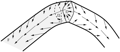
Figure 7. The gradient flow inside a one-handle. The shaded region on the boundary of the one-handle is a piece of $F$; the disk $D$ (with solid boundary, in the center) goes through the index one critical point. Its translate $D_{-}$ (with dotted boundary) does not, and the subregion of $F$ terminating in the dotted circle, when capped off by $D_{-}$, is transverse to the gradient flow.

We can perform the analogous construction at the $\alpha$-components of the boundary of $F$, only now, the $\alpha$ curve bounds a disk $D$ in $U_{0}$, which consists of points flowing out of the corresponding index two critical point. By cutting out a neighborhood of the boundary, and attaching a translate of the $D$, we once again obtain a cap which is transverse to the gradient flow $\vec{\nabla}f$.

Observe that if $x_{i}\in\mathrm{int}\mathcal{P}$, then (if we chose the above $\epsilon$ sufficiently small),

(6) $${\overline{n}}_{x_{i}}(\mathcal{P})=\#\{x\in F^{-}\big{|}\Phi(x)=x_{i}\}$$

(with the same formula holding for $z$ in place of $x_{i}$). Moreover, if $x_{i}\in\partial\mathcal{P}$, then

(7) $${\overline{n}}_{x_{i}}(\mathcal{P})=\frac{1}{2}\#\{x\in\partial F|\Phi(x)=x_{i}\}+\#\{x\in F^{-}|\Phi(x)=x_{i}\}.$$

By adding the caps as above to $F^{-}$, we construct a closed, oriented two-manifold ${\widehat{F}}$ and a map

$${\widehat{\Phi}}\colon{\widehat{F}}\longrightarrow Y,$$

which crosses the connecting trajectories between the index one and two critical points at each point $x\in F^{-}$ which maps under $\Phi$ to $x_{i}$, and similarly, ${\widehat{\Phi}}$ crosses the connecting trajectory belonging to $z$ at those $x\in F^{-}$ which map under $\Phi$ to $z$.

Away from these points, we have a canonical identification

$${\widehat{\Phi}}^{*}((\vec{\nabla}f)^{\perp})\cong\Phi^{*}(v^{\perp}).$$

By the local calculation from Lemma 7.6, it follows that

(8) $$\langle e\left({\widehat{\Phi}}^{*}(v^{\perp})\right),{\widehat{F}}\rangle=\langle e\left({\widehat{\Phi}}^{*}(\vec{\nabla}f^{\perp})\right),{\widehat{F}}\rangle+2\#\{x\in F^{-}|\Phi(x)=x_{i}\}-2\#\{x\in F^{-}|\Phi(x)=z\}.$$

(Note that the term involving $z$ follows just as in the proof of Lemma 7.6, with the difference that now the index of the vector field $v$ around the corresponding critical point in $U_{0}$ is $+1$ rather than $-1$, since the critical point has index zero rather than one.)

Moreover, the Euler number of ${\widehat{\Phi}}^{*}(\vec{\nabla}f^{\perp})$ is $\chi(\mathcal{P})$ plus the number of disks which are attached to $F^{-}$ to obtain the closed manifold ${\widehat{F}}$ (since each boundary disk is transverse to the gradient flow, so ${\vec{\nabla}f}^{\perp}$ is naturally identified with the tangent bundle of the disk, which has relative Euler number one relative to the trivialization it gets from the bounding circle). But the number of such disks is simply $\#\{x\in\partial F|\Phi(x)=x_{i}\}$. Combining this with Equations (6), (7), and (8), we obtain Equation (5), and hence proposition follows. ∎

8. Twisted Coefficients

We define here variants of the Floer homology groups constructed in [27]: these are Floer homology groups with a “twisted coefficient system.” The input here is is a three-manifold $Y$ equipped with a ${\mathrm{Spin}}^{c}$ structure $\mathfrak{s}$, and a module $M$ over the group-ring $\mathbb{Z}[H^{1}(Y;\mathbb{Z})]$. We begin with the definition in Subsection 8.1, discussing how the holomorphic triangle construction needs to be modified in Subsection 8.2

8.1. Twisted coefficients

We give first the “universal construction”, using the free module $M=\mathbb{Z}[H^{1}(Y;\mathbb{Z})]$. We need a surjective, additive assignment (in the sense of Definition LABEL:HolDiskOne:def:Additive of [27]):

$$A\colon\pi_{2}(\mathbf{x},\mathbf{y})\longrightarrow H^{1}(Y;\mathbb{Z}),$$

which is invariant under the action of $\pi_{2}(\mathrm{Sym}^{g}(\Sigma))$.

We can construct such a map as follows. A complete set of paths for $\mathfrak{s}$ in the sense of Definition LABEL:HolDiskOne:def:CompSetPath of [27] gives rise to identifications for any $i,j$:

$$\pi_{2}(\mathbf{x}_{i},\mathbf{x}_{j})\cong\pi_{2}(\mathbf{x}_{0},\mathbf{x}_{0}),$$

by

$$\phi_{i}*\pi_{2}(\mathbf{x}_{i},\mathbf{x}_{j})\cong\pi_{2}(\mathbf{x}_{0},\mathbf{x}_{0})*\phi_{j}.$$

These isomorphisms fit together in an additive manner, thanks to the associativity of $*$. We then use the splitting $\pi_{2}(\mathbf{x}_{0},\mathbf{x}_{0})\cong\mathbb{Z}\times H^{1}(Y;\mathbb{Z})$ given by the basepoint, followed by the natural projection to the second factor.

We can then define

$$\underline{\partial}^{\infty}[\mathbf{x},i]=\sum_{\mathbf{y}\in{\mathbb{T}}_{\alpha}\cap{\mathbb{T}}_{\beta}}\left(\sum_{\phi\in\pi_{2}(\mathbf{x},\mathbf{y})}\#\mathcal{M}(\phi)e^{A(\phi)}{[\mathbf{y},i-n_{z}(\phi)]}\right),$$

which is a finite sum under the strong admissibility hypotheses.

Analogous constructions work for $CF^{+}$, $CF^{-}$, and $\widehat{CF}$, as well (with, once again, weak admissibility sufficing for $CF^{+}$ and $\widehat{CF}$).

Remark 8.1.

Note that there is a “universal” coefficient system for Lagrangian Floer homology, with coefficients in a group-ring over $\pi_{1}(\Omega(L_{0},L_{1}))$. In fact, the construction we have here is a specialization of this: in our case, the fundamental group of the configuration space is $\mathbb{Z}\oplus H^{1}(Y,\mathbb{Z})$, but the $\mathbb{Z}$ summand is already implicit in our consideration of pairs $[\mathbf{x},i]\in({\mathbb{T}}_{\alpha}\cap{\mathbb{T}}_{\beta})\times\mathbb{Z}$.

It is worth noting that, although the definition of the boundary map still depends on a coherent system of orientations $\mathfrak{o}$, the isomorphism class of the chain complex as a $\mathbb{Z}$-module does not: given a homomorphism $\mu\colon H^{1}(Y;\mathbb{Z})\longrightarrow\mathbb{Z}/{2}\mathbb{Z}$, the map

(9) $$f(e^{h}[\mathbf{x},i])=(-1)^{\mu(h)}e^{h}[\mathbf{x},i]$$

gives an isomorphism from the chain complex using $\mathfrak{o}$ to the chain complex using $\mathfrak{o}^{\prime}$ with $\delta(\mathfrak{o},\mathfrak{o}^{\prime})=\mu$.

Note that as $\mathbb{Z}$-modules, all of these chain complexes have a natural relative $\mathbb{Z}$ grading, which lifts the obvious relative $\mathbb{Z}/{{\mathfrak{d}}(\mathfrak{s})}\mathbb{Z}$-grading. Specifically, given $g\otimes[\mathbf{x},i]$ and $h\otimes[\mathbf{y},j]$ with $g,h\in H^{1}(Y;\mathbb{Z})$, if we let $\phi$ be the class with $A(\phi)=g-h$ and $n_{z}(\phi)=i-j$ (this now uniquely specifies $\phi$), we let the relative grading between $g\otimes[\mathbf{x},i]$ and $h\otimes[\mathbf{y},j]$ be given by the Maslov index of $\phi$. In view of this, we can think of the corresponding homologies as analogues of a construction of Fintushel and Stern, for $\mathbb{Z}$ graded instanton homology (see [8]).

For any $\mathbb{Z}[H^{1}(Y;\mathbb{Z})]$-module $M$, we have homology groups defined by

$$\underline{HF}(Y,\mathfrak{s};M)=H_{*}\left(\underline{CF}(Y,\mathfrak{s})\otimes_{Z[H^{1}(Y;\mathbb{Z})]}M\right)$$

(where $\underline{HF}$ can be any of $\underline{HF^{\infty}}$, $\underline{HF^{+}}$, $\underline{HF^{-}}$, or $\underline{\widehat{HF}}$). The homology groups from [27] (with “untwisted coefficients”) are special cases of this construction, using the module $M=\mathbb{Z}$, thought of as the trivial $\mathbb{Z}[H^{1}(Y;\mathbb{Z})]$-module. (In fact, writing $b=b_{1}(Y)$, the $2^{b}$ different choices of orientation systems over $\mathbb{Z}$ correspond to the $2^{b}$ different module structures on $\mathbb{Z}$, induced from the $2^{b}$ ring homomorphisms $\mathbb{Z}[H^{1}(Y;\mathbb{Z})]\longrightarrow\mathbb{Z}$.)

Note also that the action of $H_{1}(Y;\mathbb{Z})/\mathrm{Tors}$ on $CF^{\infty}(Y,\mathfrak{s})$ has an interpretation in this world: the action of $\zeta\in H_{1}(Y;\mathbb{Z})$ on $[\mathbf{x},i]\in CF^{\infty}(Y,\mathfrak{s})$ as defined in Subsection LABEL:HolDiskOne:subsec:DefAct of [27] can be represented by $\langle\underline{\partial}[\mathbf{x},i],\zeta\rangle$, where the angle brackets represent the natural pairing $\mathbb{Z}[H^{1}(Y;\mathbb{Z})]\otimes(H_{1}(Y;\mathbb{Z})/\mathrm{Tors})\longrightarrow\mathbb{Z}$,

A modification of the techniques from [27] gives the following:

Theorem 8.2.

Let $Y$ be a three-manifold equipped with a ${\mathrm{Spin}}^{c}$ structure $\mathfrak{s}$ and a $\mathbb{Z}[H^{1}(Y;\mathbb{Z})]$-module $M$. Let $(\Sigma,\mbox{\boldmath$\alpha$},\mbox{\boldmath$\beta$},z)$ be a strongly $\mathfrak{s}$-admissible Heegaard diagram for $Y$. Then the groups $\underline{HF^{\infty}}(\mbox{\boldmath$\alpha$},\mbox{\boldmath$\beta$},\mathfrak{s},M)$, $\underline{HF^{+}}(\mbox{\boldmath$\alpha$},\mbox{\boldmath$\beta$},\mathfrak{s},M)$, $\underline{HF^{-}}(\mbox{\boldmath$\alpha$},\mbox{\boldmath$\beta$},\mathfrak{s},M)$, and $\underline{\widehat{HF}}(\mbox{\boldmath$\alpha$},\mbox{\boldmath$\beta$},\mathfrak{s},M)$ are invariant under changes of almost complex structures and isotopies. These groups are all modules over the group-ring $\mathbb{Z}[H^{1}(Y;\mathbb{Z})]$.

Independence of complex structure follows exactly as in [27]. For isotopy invariance, observe that an isotopy $\Psi_{t}$ as in Subsection LABEL:HolDiskOne:sec:Isotopies of [27] allows one to transfer an additive map $A$ from $\pi_{2}(\mathbf{x},\mathbf{y})$ for $\mathbf{x},\mathbf{y}\in{\mathbb{T}}_{\alpha}\cap{\mathbb{T}}_{\beta}$ to an additive map on $\pi_{2}(\mathbf{x}^{\prime},\mathbf{y}^{\prime})$ for $\mathbf{x}^{\prime},\mathbf{y}^{\prime}\in\Psi_{1}({\mathbb{T}}_{\alpha})\cap{\mathbb{T}}_{\beta}$. Stabilization follows as in [27], while to understand handleslide invariance, describe how to modify the holomorphic triangle construction to take into account the twisted coefficient system.

8.2. Triangles and twisted coefficients

To understand the triangle construction with twisted coefficients, we set up some topological preliminaries concerning relative ${\mathrm{Spin}}^{c}$ structures

8.2.1. Relative ${\mathrm{Spin}}^{c}$ structures

Continuing notation from Subsection LABEL:HolDiskOne:sec:HolTriangles of [27], let $(\Sigma,\mbox{\boldmath$\alpha$},\mbox{\boldmath$\beta$},\mbox{\boldmath$\gamma$},z)$ be a pointed Heegaard triple, and let $X_{\alpha,\beta,\gamma}$ be the induced cobordism between $Y_{\alpha,\beta}$, $Y_{\beta,\gamma}$, and $Y_{\alpha,\gamma}$. Fix ${\mathrm{Spin}}^{c}$ structures $\mathfrak{t}_{\alpha,\beta}$, $\mathfrak{t}_{\beta,\gamma}$, $\mathfrak{t}_{\alpha,\gamma}$ over the three boundary components, with $\epsilon(\mathfrak{t}_{\alpha,\beta},\mathfrak{t}_{\beta,\gamma},\mathfrak{t}_{\alpha,\gamma})=0$. Fix complete sets of paths for each of these three ${\mathrm{Spin}}^{c}$ structures (in the sense of Definition LABEL:HolDiskOne:def:CompSetPath of [27]). This gives us identifications

$$\pi_{2}(\mathbf{x}_{0},\mathbf{y}_{0},\mathbf{w}_{0})=\pi_{2}(\mathbf{x},\mathbf{y},\mathbf{w}),$$

where $\mathbf{x}_{0}$ and $\mathbf{x}$ (resp. $\mathbf{y}_{0}$ and $\mathbf{y}$, resp. $\mathbf{w}_{0}$ and $\mathbf{w}$) both represent $\mathfrak{t}_{\alpha,\beta}$ (resp. $\mathfrak{t}_{\beta,\gamma}$ resp. $\mathfrak{t}_{\alpha,\gamma}$).

In effect, this allows us to think of $\pi_{2}(\mathbf{x}_{0},\mathbf{y}_{0},\mathbf{w}_{0})$ as an affine space for $H^{2}(X,Y;\mathbb{Z})$ (c.f. Proposition LABEL:HolDiskOne:prop:CalcPiTwo of [27]), which maps onto the space of ${\mathrm{Spin}}^{c}$ structures extending $\mathfrak{t}_{\alpha,\beta}$, $\mathfrak{t}_{\beta,\gamma}$, $\mathfrak{t}_{\alpha,\gamma}$ (c.f. Proposition LABEL:HolDiskOne:prop:SpinCForTriangles of [27]). When thinking of $\pi_{2}(\mathbf{x}_{0},\mathbf{y}_{0},\mathbf{w}_{0})$ in this manner, we refer to it as a space of relative ${\mathrm{Spin}}^{c}$ structures, and denote it by $\underline{{\mathrm{Spin}}^{c}}(X_{\alpha,\beta,\gamma})$.

The subset of $\underline{{\mathrm{Spin}}^{c}}(X_{\alpha,\beta,\gamma})$ representing a fixed (absolute) ${\mathrm{Spin}}^{c}$ structure structure $\mathfrak{s}_{\alpha,\beta,\gamma}$ will be denoted ${\mathrm{Spin}}^{c}(X_{\alpha,\beta,\gamma};\mathfrak{s}_{\alpha,\beta,\gamma})$.

We will use this terminology for higher polygons, as well.

8.2.2. The maps with twisted coefficients

The space of relative ${\mathrm{Spin}}^{c}$ structures $\underline{{\mathrm{Spin}}^{c}}(X_{\alpha,\beta,\gamma};\mathfrak{s}_{\alpha,\beta,\gamma})$ (which induce a given ${\mathrm{Spin}}^{c}$ structure $\mathfrak{s}_{\alpha,\beta,\gamma}$ over $X_{\alpha,\beta,\gamma}$) is a space with a natural action of $H^{1}(Y_{\alpha,\beta};\mathbb{Z})\times H^{1}(Y_{\beta,\gamma};\mathbb{Z})\times H^{1}(Y_{\alpha,\gamma};\mathbb{Z})$. As such, it can be used to induce an $H^{1}(Y_{\alpha,\gamma};\mathbb{Z})$-module from a pair $M_{\alpha,\beta}$ and $M_{\beta,\gamma}$ of $H^{1}(Y_{\alpha,\beta};\mathbb{Z})$ and $H^{1}(Y_{\beta,\gamma};\mathbb{Z})$-modules:

$$\left\{M_{\alpha,\beta}\otimes M_{\beta,\gamma}\right\}^{\mathfrak{s}_{\alpha,\beta,\gamma}}=\frac{(m_{\alpha,\beta},m_{\beta,\gamma},\underline{\mathfrak{s}})\in M_{\alpha,\beta}\times M_{\beta,\gamma}\times\underline{{\mathrm{Spin}}^{c}}(X_{\alpha,\beta,\gamma},\mathfrak{s}_{\alpha,\beta,\gamma})}{(m_{\alpha,\beta},m_{\beta,\gamma},\underline{\mathfrak{s}})\sim(h_{\alpha,\beta}\cdot m_{\alpha,\beta},h_{\beta,\gamma}\cdot m_{\beta,\gamma},(h_{\alpha,\beta}\times h_{\beta,\gamma}\times 0)\cdot\underline{\mathfrak{s}})},$$

where $h_{\alpha,\beta}$ and $h_{\beta,\gamma}$ are arbitrary elements of $H^{1}(Y_{\alpha,\beta};\mathbb{Z})$ and $H^{1}(Y_{\beta,\gamma};\mathbb{Z})$ respectively.

Fix a ${\mathrm{Spin}}^{c}$ structure $\mathfrak{s}$ over $X_{\alpha,\beta,\gamma}$, whose restriction to $Y_{\alpha,\beta}$ and $Y_{\beta,\gamma}$ is $\mathfrak{t}_{\alpha,\beta}$ and $\mathfrak{t}_{\beta,\gamma}$ respectively. We can now define a map

$$\underline{f^{\infty}_{\alpha,\beta,\gamma}}(~{}\cdot~{},\mathfrak{s})\colon\underline{CF^{\infty}}(Y_{\alpha,\beta},\mathfrak{t}_{\alpha,\beta};M_{\alpha,\beta})\otimes\underline{CF^{\infty}}(Y_{\beta,\gamma},\mathfrak{t}_{\beta,\gamma};M_{\beta,\gamma})$$

$$\hskip 144.54pt\longrightarrow\underline{CF^{\infty}}(Y_{\alpha,\gamma},\mathfrak{t}_{\alpha,\gamma};\left\{M_{\alpha,\beta}\otimes M_{\beta,\gamma}\right\}^{\mathfrak{s}}),$$

by the formula:

(10) $$\underline{f^{\infty}_{\alpha,\beta,\gamma}}(m_{\alpha,\beta}[\mathbf{x},i]\otimes m_{\beta,\gamma}[\mathbf{y},j];\mathfrak{s})=$$

$$\sum_{\mathbf{w}\in{\mathbb{T}}_{\alpha}\cap{\mathbb{T}}_{\beta}}\sum_{\{\psi\in\pi_{2}(\mathbf{x},\mathbf{y},\mathbf{w})\big{|}\mathfrak{s}_{z}(\psi)=\mathfrak{s}\}}\left(\#\mathcal{M}(\psi)\right)\{m_{\alpha,\beta}\otimes m_{\beta,\gamma}\otimes\underline{\mathfrak{s}}_{z}(\psi)\}\cdot[\mathbf{w},i+j-n_{z}(\psi)].$$

The braces above indicate the natural map

$$\left\{\cdot\otimes\cdot\otimes\cdot\right\}\colon M_{\alpha,\beta}\otimes M_{\beta,\gamma}\otimes\underline{{\mathrm{Spin}}^{c}}(X_{\alpha,\beta,\gamma},\mathfrak{s})\longrightarrow\{M_{\alpha,\beta}\otimes M_{\beta,\gamma}\}^{\mathfrak{s}}.$$

The following analogue of Theorem LABEL:HolDiskOne:thm:HolTriangles of [27] holds in the present context:

Theorem 8.3.

Let $(\Sigma,\mbox{\boldmath$\alpha$},\mbox{\boldmath$\beta$},\mbox{\boldmath$\gamma$},z)$ be a pointed Heegaard triple-diagram, which is strongly $\mathfrak{s}$-admissible for some ${\mathrm{Spin}}^{c}$ structure $\mathfrak{s}$ over the underlying four-manifold $X$, and fix modules $M_{\alpha,\beta}$ and $M_{\beta,\gamma}$ for $H^{1}(Y_{\alpha,\beta};\mathbb{Z})$ and $H^{1}(Y_{\beta,\gamma};\mathbb{Z})$ respectively. Then the sum on the right-hand-side of Equation (10) is finite, giving rise to a chain map which also induces maps on homology:

$$\underline{F^{\infty}_{\alpha,\beta,\gamma}}(\cdot,\mathfrak{s}_{\alpha,\beta,\gamma})\colon\underline{HF^{\infty}}(Y_{\alpha,\beta},\mathfrak{t}_{\alpha,\beta};M_{\alpha,\beta})\otimes\underline{HF^{\infty}}(Y_{\beta,\gamma},\mathfrak{t}_{\beta,\gamma};M_{\beta,\gamma})$$

$$\hskip 144.54pt\longrightarrow\underline{HF^{\infty}}(Y_{\alpha,\gamma},\mathfrak{t}_{\alpha,\gamma};\{M_{\alpha,\beta}\otimes M_{\beta,\gamma}\}^{\mathfrak{s}_{\alpha,\beta,\gamma}})$$

$$\underline{F^{\leq 0}_{\alpha,\beta,\gamma}}(\cdot,\mathfrak{s}_{\alpha,\beta,\gamma})\colon\underline{HF^{\leq 0}}(Y_{\alpha,\beta},\mathfrak{t}_{\alpha,\beta};M_{\alpha,\beta})\otimes\underline{HF^{\leq 0}}(Y_{\beta,\gamma},\mathfrak{t}_{\beta,\gamma};M_{\beta,\gamma})$$

$$\hskip 144.54pt\longrightarrow\underline{HF^{\leq 0}}(Y_{\alpha,\gamma},\mathfrak{t}_{\alpha,\gamma};\{M_{\alpha,\beta}\otimes M_{\beta,\gamma}\}^{\mathfrak{s}_{\alpha,\beta,\gamma}}).$$

The induced chain map

$$\underline{f^{+}_{\alpha,\beta,\gamma}}(\cdot,\mathfrak{s}_{\alpha,\beta,\gamma})\colon\underline{CF^{+}}(Y_{\alpha,\beta},\mathfrak{t}_{\alpha,\beta};M_{\alpha,\beta})\otimes\underline{CF^{\leq 0}}(Y_{\beta,\gamma},\mathfrak{t}_{\beta,\gamma};M_{\beta,\gamma})$$

$$\hskip 144.54pt\longrightarrow\underline{CF^{+}}(Y_{\alpha,\gamma},\mathfrak{t}_{\alpha,\gamma};\{M_{\alpha,\beta}\otimes M_{\beta,\gamma}\}^{\mathfrak{s}_{\alpha,\beta,\gamma}})$$

gives a well-defined chain map when the triple diagram is only weakly admissible, and the Heegaard diagram $(\Sigma,\mbox{\boldmath$\beta$},\mbox{\boldmath$\gamma$},z)$ is strongly admissible for $\mathfrak{t}_{\beta,\gamma}$. In fact, the induced map

$$\underline{{\widehat{f}}_{\alpha,\beta,\gamma}}(\cdot,\mathfrak{s}_{\alpha,\beta,\gamma})\colon\underline{\widehat{CF}}(Y_{\alpha,\beta},\mathfrak{t}_{\alpha,\beta};M_{\alpha,\beta})\otimes\underline{\widehat{CF}}(Y_{\beta,\gamma},\mathfrak{t}_{\beta,\gamma};M_{\beta,\gamma})$$

$$\hskip 144.54pt\longrightarrow\underline{\widehat{CF}}(Y_{\alpha,\gamma},\mathfrak{t}_{\alpha,\gamma};\{M_{\alpha,\beta}\otimes M_{\beta,\gamma}\}^{\mathfrak{s}_{\alpha,\beta,\gamma}})$$

gives a well-defined chain map when the diagram is weakly admissible. There are induced maps on homology:

$$\underline{{\widehat{F}}_{\alpha,\beta,\gamma}}(\cdot,\mathfrak{s}_{\alpha,\beta,\gamma})\colon\underline{\widehat{HF}}(Y_{\alpha,\beta},\mathfrak{t}_{\alpha,\beta};M_{\alpha,\beta})\otimes\widehat{HF}(Y_{\beta,\gamma},\mathfrak{t}_{\beta,\gamma};M_{\beta,\gamma})$$

$$\hskip 144.54pt\longrightarrow\widehat{HF}(Y_{\alpha,\gamma},\mathfrak{t}_{\alpha,\gamma};\{M_{\alpha,\beta}\otimes M_{\beta,\gamma}\}^{\mathfrak{s}_{\alpha,\beta,\gamma}})$$

$$F^{+}_{\alpha,\beta,\gamma}(\cdot,\mathfrak{s}_{\alpha,\beta,\gamma})\colon\underline{HF^{+}}(Y_{\alpha,\beta},\mathfrak{t}_{\alpha,\beta})\otimes\underline{HF}^{\leq 0}(Y_{\beta,\gamma},\mathfrak{t}_{\beta,\gamma})$$

$$\hskip 144.54pt\longrightarrow\underline{HF^{+}}(Y_{\alpha,\gamma},\mathfrak{t}_{\alpha,\gamma};\{M_{\alpha,\beta}\otimes M_{\beta,\gamma}\}^{\mathfrak{s}_{\alpha,\beta,\gamma}})).$$

Independence of complex structure and isotopy invariance of this map proceeds exactly as in [27] (c.f. Propositions LABEL:HolDiskOne:prop:TrianglesJIndep and LABEL:HolDiskOne:prop:TriangleIsotopyInvariance of [27] respectively). Associativity, on the other hand, can be given a the following sharper statement.

Observe first that there is a canonical gluing

$$\underline{{\mathrm{Spin}}^{c}}(X_{\alpha,\beta,\gamma},\mathfrak{s}_{\alpha,\beta,\gamma})\times\underline{{\mathrm{Spin}}^{c}}(X_{\alpha,\gamma,\delta},\mathfrak{s}_{\alpha,\gamma,\delta})\longrightarrow\underline{{\mathrm{Spin}}^{c}}(X_{\alpha,\beta,\gamma,\delta})$$

which maps onto the set of all relative ${\mathrm{Spin}}^{c}$ structures over $X_{\alpha,\beta,\gamma,\delta}$ whose restrictions to $X_{\alpha,\beta,\gamma}$ and $X_{\alpha,\gamma,\delta}$ represent ${\mathrm{Spin}}^{c}$ structures $\mathfrak{s}_{\alpha,\beta,\gamma}$ and $\mathfrak{s}_{\alpha,\gamma,\delta}$ respectively. Thus, the set of ${\mathrm{Spin}}^{c}$ induced structures in $X_{\alpha,\beta,\gamma,\delta}$ under this map consists of a $\delta H^{1}(Y;\mathbb{Z})$-orbit. Using this gluing, we obtain an identification

$$\{\{M_{\alpha,\beta}\otimes M_{\beta,\gamma}\}^{\mathfrak{s}_{\alpha,\beta,\gamma}}\otimes M_{\gamma,\delta}\}^{\mathfrak{s}_{\alpha,\beta,\delta}}$$

$$\cong \coprod_{\{\mathfrak{s}\in{\mathrm{Spin}}^{c}(X_{\alpha,\beta,\gamma,\delta})\big{|}\mathfrak{s}|X_{\alpha,\beta,\gamma}=\mathfrak{s}_{\alpha,\beta,\gamma},\mathfrak{s}|X_{\alpha,\gamma,\delta}=\mathfrak{s}_{\alpha,\gamma,\delta}\}}\{M_{\alpha,\beta}\otimes M_{\beta,\gamma}\otimes M_{\gamma,\delta}\}^{\mathfrak{s}},$$

where $\left\{M_{\alpha,\beta}\otimes M_{\beta,\gamma}\otimes M_{\gamma,\delta}\right\}^{\mathfrak{s}}$ denotes the $H^{1}(Y_{\alpha,\delta};\mathbb{Z})$-module induced from $M_{\alpha,\beta}$, $M_{\beta,\gamma}$, $M_{\gamma,\delta}$ and the set of relative ${\mathrm{Spin}}^{c}$ structures inducing the given ${\mathrm{Spin}}^{c}$ structure $\mathfrak{s}$ over the four-manifold $X_{\alpha,\beta,\gamma,\delta}$.

Theorem 8.4.

Let $(\Sigma,\mbox{\boldmath$\alpha$},\mbox{\boldmath$\beta$},\mbox{\boldmath$\gamma$},\mbox{\boldmath$\delta$},z)$ be a pointed Heegaard quadruple which is strongly ${\mathfrak{S}}$-admissible, where ${\mathfrak{S}}$ is a $\delta H^{1}(Y_{\beta,\delta})+\delta H^{1}(Y_{\alpha,\gamma})$-orbit in ${\mathrm{Spin}}^{c}(X_{\alpha,\beta,\gamma,\delta})$. Fix also modules $M_{\alpha,\beta}$, $M_{\beta,\gamma}$, and $M_{\gamma,\delta}$ for $H^{1}(Y_{\alpha,\beta};\mathbb{Z})$, $H^{1}(Y_{\beta,\gamma};\mathbb{Z})$, $H^{1}(Y_{\beta,\gamma};\mathbb{Z})$, and $H^{1}(Y_{\gamma,\delta};\mathbb{Z})$ respectively.

Then,

$$\sum_{\mathfrak{s}\in{\mathfrak{S}}}\underline{F^{*}_{\alpha,\gamma,\delta}}(\underline{F^{*}_{\alpha,\beta,\gamma}}(\xi_{\alpha,\beta}\otimes\theta_{\beta,\gamma};\mathfrak{s}_{\alpha,\beta,\gamma})\otimes\theta_{\gamma,\delta};\mathfrak{s}_{\alpha,\gamma,\delta})$$

$$= \sum_{\mathfrak{s}\in{\mathfrak{S}}}\underline{F^{*}_{\alpha,\beta,\delta}}(\xi_{\alpha,\beta}\otimes\underline{F^{\leq 0}_{\beta,\gamma,\delta}}(\theta_{\beta,\gamma}\otimes\theta_{\gamma,\delta};\mathfrak{s}_{\beta,\gamma,\delta});\mathfrak{s}_{\alpha,\beta,\delta}),$$

where $\underline{F^{*}}=\underline{F^{\infty}}$, $\underline{F^{+}}$ or $\underline{F^{-}}$; also,

$$\sum_{\mathfrak{s}\in{\mathfrak{S}}}\underline{{\widehat{F}}_{\alpha,\gamma,\delta}}(\underline{{\widehat{F}}_{\alpha,\beta,\gamma}}(\xi_{\alpha,\beta}\otimes\theta_{\beta,\gamma};\mathfrak{s}_{\alpha,\beta,\gamma})\otimes\theta_{\gamma,\delta};\mathfrak{s}_{\alpha,\gamma,\delta})$$

$$= \sum_{\mathfrak{s}\in{\mathfrak{S}}}\underline{{\widehat{F}}_{\alpha,\beta,\delta}}(\xi_{\alpha,\beta}\otimes\underline{{\widehat{F}}_{\beta,\gamma,\delta}}(\theta_{\beta,\gamma}\otimes\theta_{\gamma,\delta};\mathfrak{s}_{\beta,\gamma,\delta});\mathfrak{s}_{\alpha,\beta,\delta}),$$

where we are taking coefficients in coefficients in $\coprod_{\mathfrak{s}\in{\mathfrak{S}}}\{M_{\alpha,\beta}\otimes M_{\beta,\gamma}\otimes M_{\gamma,\delta}\}^{\mathfrak{s}}$ over $Y_{\alpha,\delta}$.

Proof. The proof is the same as the proof of Theorem LABEL:HolDiskOne:thm:Associativity of [27], only keeping track now of the homotopy classes of the corresponding triangles.         

8.2.3. Handleslide invariance

With the holomorphic triangles in place, the proof of handleslide invariance proceeds as it did in [27], with the following remarks.

Recall that the map given by a handleslide (as in Theorem LABEL:HolDiskOne:thm:HandleslideInvariance of [27]) is induced from a Heegaard triple $(\Sigma,\mbox{\boldmath$\alpha$},\mbox{\boldmath$\beta$},\mbox{\boldmath$\gamma$},z)$, which represents the cobordism $X_{\alpha,\beta,\gamma}$ obtained from $[0,1]\times Y$ by deleting a bouquet of circles. Here, $Y_{\alpha,\beta}\cong Y$, $Y_{\beta,\gamma}\cong\#^{g}(S^{1}\times S^{2})$, and $Y_{\alpha,\gamma}\cong Y$. Now, our input includes an arbitrary $\mathbb{Z}[H^{1}(Y;\mathbb{Z})]$ module $M$. For the handleslide map, we consider the trivial $H^{1}(Y_{\beta,\gamma};\mathbb{Z})$-module $M_{\beta,\gamma}\cong\mathbb{Z}$ (so that $\underline{HF^{\leq 0}}(Y_{\beta,\gamma},M)\cong HF^{\leq 0}(\#^{g}(S^{1}\times S^{2}))$ is equipped with its top-dimensional generator $\Theta_{\beta,\gamma}$). It is easy to see that for this choice of $M_{\beta,\gamma}$, there is also a canonical identification of $\mathbb{Z}[H^{1}(Y;\mathbb{Z})]$-modules

$$M\cong\{M\otimes M_{\beta,\gamma}\},$$

where the pairing here uses the cobordism $X_{\alpha,\beta,\gamma}$.

9. Surgery exact sequences

We investigate how surgeries on a three-manifold affect its invariants. We consider first the effect on $HF^{+}$ of $+1$ surgeries on integral homology three-spheres, then a generalization which holds for arbitrary (closed, oriented) three-manifolds, and then the case of fractional $1/q$-surgeries on an integral homology three-sphere. This latter case uses the homology theories with twisted coefficients. We then give analogous results for $\widehat{HF}$. After this, we present a surgery formula for integer surgeries. In the final subsection, we consider a $+1$ surgery formula with twisted coefficients.

9.1. $+1$ surgeries on an integral homology three-sphere

We start with the case of a homology three-sphere $Y$. Let $K\subset Y$ be a knot. Let $Y_{0}$ be the manifold obtained by $0$-surgery on $K$, and $Y_{1}$ be obtained by $(+1)$-surgery. Let

$$HF^{+}(Y_{0})\cong\bigoplus_{\mathfrak{s}\in{\mathrm{Spin}}^{c}(Y_{0})}HF^{+}(Y_{0},\mathfrak{s}),$$

viewed as a $\mathbb{Z}/{2}\mathbb{Z}$-relatively graded group. In fact, we will view the homology groups $HF^{+}(Y)$ and $HF^{+}(Y_{1})$ as $\mathbb{Z}/{2}\mathbb{Z}$-graded, as well.

Theorem 9.1.

There is a $U$-equivariant exact sequence of relatively $\mathbb{Z}/{2}\mathbb{Z}$-graded complexes:

$$\begin{CD}...@>{}>{}>HF^{+}(Y)@>{F_{1}}>{}>HF^{+}(Y_{0})@>{F_{2}}>{}>HF^{+}(Y_{1})@>{F_{3}}>{}>...\end{CD}$$

In fact, if we give $HF^{+}(Y)$ and $HF^{+}(Y_{1})$ absolute $\mathbb{Z}/{2}\mathbb{Z}$-gradings so that $\chi(\widehat{HF}(Y))=\chi(\widehat{HF}(Y_{1}))=+1$, then $F_{3}$ preserves degree.

The maps in Theorem 9.1 are constructed with the help of holomorphic triangles. Thus, we must construct compatible Heegaard decompositions for all three manifolds $Y$, $Y_{0}$, and $Y_{1}$. Exactness is then proved using a filtration on the homology groups above, together with the homological-algebraic constructions used in establishing the surgery sequences for instanton Floer homology (see [10], [4]). The proof occupies the rest of the present subsection.

Lemma 9.2.

There is a pointed Heegaard multi-diagram

$$(\Sigma,\mbox{\boldmath$\alpha$},\mbox{\boldmath$\beta$},\mbox{\boldmath$\gamma$},\mbox{\boldmath$\delta$},z)$$

with the property that

• the Heegaard diagrams $(\Sigma,\mbox{\boldmath$\alpha$},\mbox{\boldmath$\beta$})$, $(\Sigma,\mbox{\boldmath$\alpha$},\mbox{\boldmath$\gamma$})$, and $(\Sigma,\mbox{\boldmath$\alpha$},\mbox{\boldmath$\delta$})$ describe $Y$, $Y_{0}$, and $Y_{1}$ respectively,

• for each $i=1,...,g-1$, the curves $\beta_{i}$, $\gamma_{i}$, and $\delta_{i}$ are small isotopic translates of one another, each pairwise intersecting in a pair of canceling transverse intersection points (where the isotopies are supported in the complement of $z$),

• the curve $\gamma_{g}$ is isotopic to the juxtaposition of $\delta_{g}$ and $\beta_{g}$ (with appropriate orientations),

• every non-trivial multi-periodic domain has both positive and negative coefficients.

Proof. Consider a Morse function on $Y-{\mathrm{nd}}(K)$ with one index zero critical point, $g$ index one critical points and $g-1$ index two critical points. Let $\Sigma$ be the $3/2$-level of this function, $\alpha$ be the curves where $\Sigma$ meets the ascending manifolds of the index one critical points in $\Sigma$, and let $\beta_{1},...,\beta_{g-1}$ be the curves where $\Sigma$ meets the descending manifolds of the index two critical points. By gluing in the solid torus in three possible ways, we get the manifolds $Y$, $Y_{0}$, $Y_{1}$. Extending the given Morse function to the glued in solid tori, (by introducing an additional index two and index three critical point), we obtain Heegaard decompositions for the manifolds $Y$, $Y_{0}$, and $Y_{1}$. We let $\gamma_{i}$ and $\delta_{i}$ be small perturbations of $\beta_{i}$ for $i=1,...,g-1$. In this manner, we have satisfied Properties (1)-(3).

To satisfy Property (4), we wind to achieve weak admissibility for all ${\mathrm{Spin}}^{c}$ structures for the Heegaard subdiagram $(\Sigma,\mbox{\boldmath$\alpha$},\mbox{\boldmath$\gamma$},z)$: in fact, we can use a volume form over $\Sigma$ for which all such doubly-periodic domains have zero signed area (c.f. Lemma LABEL:HolDiskOne:lemma:EnergyZero of [27]). Then, for the $\{\beta_{1},...\beta_{g-1}\}$ and $\{\delta_{1},...,\delta_{g-1}\}$, we use small Hamiltonian translates of the $\{\gamma_{1},...,\gamma_{g-1}\}$ (ensuring that the corresponding new periodic domains each have zero energy). There is a triply-periodic domain which forms the homology between $\beta_{g}$, $\gamma_{g}$, and $\delta_{g}$ in a torus summand of $\Sigma$ containing no other $\beta_{i}$ or $\gamma_{i}$ (for $i\neq g$). By adjusting the areas of the two triangles with non-zero area, we can arrange for the signed area of the triply-periodic domain to vanish.

Figure 8. This picture takes place in the torus, with the usual edge identifications. The integers denote multiplicities for a triply-periodic domain.

    

For $i=1,...,g-1$, label

$$y_{i}^{\pm}=\beta_{i}\cap\gamma_{i},~{}~{}~{}~{}~{}~{}~{}~{}v_{i}^{\pm}=\gamma_{i}\cap\delta_{i},~{}~{}~{}~{}~{}~{}~{}~{}w_{i}^{\pm}=\beta_{i}\cap\delta_{i},$$

where the sign indicates the sign of the intersection point. Also, let

$$y_{g}=\beta_{g}\cap\gamma_{g},~{}~{}~{}~{}~{}~{}~{}~{}v_{g}=\gamma_{g}\cap\delta_{g},~{}~{}~{}~{}~{}~{}~{}~{}w_{g}=\beta_{g}\cap\delta_{g}.$$

Then, let $\Theta_{\beta,\gamma}=\{y_{1}^{+},...,y^{+}_{g-1},y_{g}\}$, $\Theta_{\gamma,\delta}=\{v_{1}^{+},...,v^{+}_{g-1},v_{g}\}$, $\Theta_{\beta,\delta}=\{w_{1}^{+},...,w^{+}_{g-1},w_{g}\}$ denote the corresponding intersection points between ${\mathbb{T}}_{\beta}\cap{\mathbb{T}}_{\gamma}$, ${\mathbb{T}}_{\gamma}\cap{\mathbb{T}}_{\delta}$ and ${\mathbb{T}}_{\beta}\cap{\mathbb{T}}_{\delta}$. (See Figure 9 for an illustration.)

Proposition 9.3.

The elements $\theta_{\beta,\gamma}=[\Theta_{\beta,\gamma},0]$, $\theta_{\gamma,\delta}=[\Theta_{\gamma,\delta},0]$, $\theta_{\beta,\delta}=[\Theta_{\beta,\delta},0]$ are cycles in $CF^{\infty}({\mathbb{T}}_{\beta},{\mathbb{T}}_{\gamma})$, $CF^{\infty}({\mathbb{T}}_{\gamma},{\mathbb{T}}_{\delta})$ and $CF^{\infty}({\mathbb{T}}_{\beta},{\mathbb{T}}_{\delta})$ respectively.

Proof. Note that the three-manifolds described here are $(g-1)$-fold connected sums of $S^{1}\times S^{2}$, so the result follows from Proposition 6.4 (or, alternatively, see Section LABEL:HolDiskOne:sec:HandleSlides of [27]).         

We can reduce the study of holomorphic triangles belonging to $X_{\beta,\gamma,\delta}$ to holomorphic triangles in the first symmetric product of the two-torus, with the help of the following analogue of the gluing theory used to establish stabilization invariance of the Floer homology groups.

Theorem 9.4.

Fix a pair of Heegaard diagrams

$$(\Sigma,\mbox{\boldmath$\beta$},\mbox{\boldmath$\gamma$},\mbox{\boldmath$\delta$},z) (E,\beta_{0},\gamma_{0},\delta_{0},z_{0}),$$ and

where $E$ is a Riemann surface of genus one. We will form the connected sum $\Sigma\#E$, where the connected sum points are near the distinguished points $z$ and $z_{0}$ respectively. Fix intersection points $\mathbf{x},\mathbf{y},\mathbf{w}$ for the first diagram and a class $\psi\in\pi_{2}(\mathbf{x},\mathbf{y},\mathbf{w})$, and intersection points $x_{0}$, $y_{0}$, and $w_{0}$ for the second, with a triangle $\psi_{0}\in\pi_{2}(x_{0},y_{0},w_{0})$ with $\mu(\psi)=\mu(\psi_{0})=0$. Suppose moreover that $n_{z_{0}}(\psi_{0})=0$. Then, for a suitable choice of complex structures and perturbations, we have a diffeomorphism of moduli spaces:

$$\mathcal{M}(\psi^{\prime})\cong\mathcal{M}(\psi)\times\mathcal{M}(\psi_{0}),$$

where $\psi^{\prime}\in\pi_{2}(\mathbf{x}\times x_{0},\mathbf{y}\times y_{0},\mathbf{w}\times w_{0})$ is the triangle for $\Sigma\#E$ whose domain on the $\Sigma$-side agrees with ${\mathcal{D}}(\psi)$, and whose domain on the $E$-side agrees with ${\mathcal{D}}(\psi_{0})+n_{z}(\psi)[E]$.

Proof. The proof is obtained by suitably modifying Theorem LABEL:HolDiskOne:thm:Gluing of [27].

Suppose that $u$ and $u_{0}$ are holomorphic representatives of $\psi$ and $\psi_{0}$ respectively. We obtain a nodal pseudo-holomorphic disk $u\vee u_{0}$ in the singular space $\mathrm{Sym}^{g+1}(\Sigma\vee E)$ specified as follows:

• At the stratum $\mathrm{Sym}^{g}(\Sigma)\times\mathrm{Sym}^{1}(E)$, $u\vee u_{0}$ is the product map $u\times u_{0}$.

• At the stratum $\mathrm{Sym}^{g-1}(\Sigma)\times\mathrm{Sym}^{2}(E)$, $u\vee u_{0}$ is given by $n_{z}(\psi)$ pseudo-holomorphic spheres which are constant on the first factor. More precisely, for each $p\in\Delta$ for which $u(p)=\{z,x_{2},...,x_{g}\}$ (where the $x_{i}\in\Sigma-\{z\}$ are arbitrary), there is a component of $u\vee u_{0}$ mapping into $\mathrm{Sym}^{g-1}(\Sigma)\times\mathrm{Sym}^{2}(E)$, consisting of the product of the constant map $\{x_{2},...,x_{g}\}$ with the sphere in $\mathrm{Sym}^{2}(E)$ which passes through $\{z\}\times u_{0}(p)$.

• The map $u\vee u_{0}$ misses all other strata of $\mathrm{Sym}^{g+1}(\Sigma\vee E)$.

As in Theorem LABEL:HolDiskOne:thm:Gluing of [27], we can splice to obtain an approximately holomorphic disk $u\#u_{0}$ (a triangle) in $\mathrm{Sym}^{g+1}(\Sigma\#E)$. When the connected sum tube is sufficiently long, the the inverse function theorem can be used to find the nearby pseudo-holomorphic triangle. The domain belonging to $u\#u_{0}$ is clearly given by $\psi\#\psi_{0}$ described above. Conversely, by Gromov’s compactness (see also Proposition LABEL:HolDiskOne:prop:GromovCompactness of [27]), any sequence of pseudo-holomorphic representatives $u_{i}\in\pi_{2}(\mathbf{x}\times x_{0},\mathbf{y}\times y_{0},\mathbf{w}\times w_{0})$ for arbitrarily long connected sum neck must limit to a pseudo-holomorphic representative for $\psi^{\prime}\#\psi_{0}^{\prime}$, where ${\mathcal{D}}(\psi_{0}^{\prime})-{\mathcal{D}}(\psi_{0})=k[E]$ for some $0\leq k\leq n_{z}(\psi)$. However, since $\pi_{2}(E)=0$, it follows that $k=0$. Thus, the gluing map covers the moduli space.         

Proposition 9.5.

There are homotopy classes of triangles $\{\psi_{k}^{\pm}\}_{k=1}^{\infty}$ in $\pi_{2}(\Theta_{\beta,\gamma},\Theta_{\gamma,\delta},\Theta_{\beta,\delta})$ for the triple-diagram $(\Sigma,\mbox{\boldmath$\beta$},\mbox{\boldmath$\gamma$},\mbox{\boldmath$\delta$},z)$ satisfying the following properties:

$$\mu(\psi^{\pm}_{k}) = 0,$$

$$n_{z}(\psi^{\pm}_{k}) = \frac{k(k-1)}{2}.$$

Moreover, each triangle in $\pi_{2}(\Theta_{\beta,\gamma},\Theta_{\gamma,\delta},\Theta_{\beta,\delta})$ is ${\mathrm{Spin}}^{c}$ equivalent to some $\psi^{\pm}_{k}$. Furthermore, there is a choice of perturbations and complex structure on $\Sigma$ with the property that for each $\Psi\in\pi_{2}(\Theta_{\beta,\gamma},\Theta_{\gamma,\delta},\mathbf{x})$ (where $\mathbf{x}\in{\mathbb{T}}_{\beta}\cap{\mathbb{T}}_{\delta}$) with $\mu(\Psi)=0$, we have that

$$\#\mathcal{M}(\Psi)=\left\{\begin{array}[]{ll}\pm 1&{\text{if $\Psi\in\{\psi^{\pm}_{k}\}_{k=1}^{\infty}$}}\\ 0&{\text{otherwise}}\end{array}\right..$$

Proof. First observe that the space of ${\mathrm{Spin}}^{c}$ structures over $X_{\beta,\gamma,\delta}$ extending a given one on the boundary is identified with $\mathbb{Z}$. In particular, modulo doubly-periodic domains for the three boundary three-manifolds, every triangle $\psi\in\pi_{2}(\Theta_{\beta,\gamma},\Theta_{\gamma,\delta},\Theta_{\beta,\delta})$ can uniquely be written as $\psi_{1}+a[S]+b[\mathcal{P}]$ for some pair of integers $a$ and $b$, where $\mathcal{P}$ is the generator of the space of triply-periodic domains: in fact, the integer $a$ is determined by the intersection number $n_{z}$, and $b$ can be determined by the signed number of times the arc in $\beta_{g}$ obtained by restricting $\psi$ to its boundary crosses some fixed $\tau\in\beta_{g}$. For the triangles $\{\psi_{k}^{\pm}\}$ this signed count can be any arbitrary integer, so these triangles represent all possible ${\mathrm{Spin}}^{c}$-equivalence classes of triangles.

The other claims are straightforward in the case where $g=1$. In this case, the curves $\beta$, $\gamma$, $\delta$ lie in a surface of genus one, so the holomorphic triangle can be lifted to the complex plane. Hence, by standard complex analysis, it is smoothly cut out, and unique.

The fact that $\#\mathcal{M}(\psi_{k}^{\pm})=\pm 1$ for higher genus follows from induction, and the gluing result, Theorem 9.4. Specifically, if the result is known for genus $g$, then we can add a new torus $E$ to $\Sigma$ which contains three curves $\beta_{0}$, $\gamma_{0}$, $\delta_{0}$ which are small Hamiltonian translates of one another (and the basepoint is chosen outside the support of the isotopy). The torus $E$ contains a standard small triangle $\psi_{0}\in\pi_{2}(y_{0}^{+},v_{0}^{+},w_{0}^{+})$, for which it is clear that $\#\mathcal{M}(\psi_{0})=1$. Gluing this triangle to the $\{\psi_{k}^{\pm}\}$ in $\Sigma$, we obtain corresponding triangles in $\Sigma\#E$ satisfying all the above hypotheses.

The fact that $\#\mathcal{M}(\Psi)=0$ for $\Psi\not\in\{\psi_{k}^{\pm}\}_{k=1}^{\infty}$ follows similarly, with the observation that the other moduli spaces of triangles on the torus are empty.         

We can define the map

$$F_{1}\colon HF^{+}(Y)\longrightarrow HF^{+}(Y_{0})$$

by summing:

$$F_{1}(\xi)=\sum_{\mathfrak{s}\in{\mathrm{Spin}}^{c}(X_{\alpha,\beta,\gamma})}\pm F^{+}_{\alpha,\beta,\gamma}(\xi\otimes\theta_{\beta,\gamma},\mathfrak{s}).$$

On the chain level, $F_{1}$ is induced from a map:

$$f_{1}([\mathbf{x},i])=\sum_{\mathbf{w}\in{\mathbb{T}}_{\alpha}\cap{\mathbb{T}}_{\gamma}}\sum_{\{\psi\in\pi_{2}(\mathbf{x},\Theta_{\beta,\gamma},\mathbf{w})\big{|}\mu(\psi)=0\}}\left(\#\mathcal{M}(\psi)\right)\cdot[\mathbf{w},i-n_{z}(\psi)],$$

where $\#\mathcal{M}(\psi)$ is calculated with respect to a particular choice of coherent orientation system (see Proposition 9.6 below). It is important to note here that the sum on the right hand side will have only finitely many non-zero elements for each fixed $\xi\in CF^{+}(Y)$. The reason for this is that all the multi-periodic domains have both positive and negative coefficients. Similarly, we define

$$f_{2}([\mathbf{x},i])=\sum_{\{\psi\in\pi_{2}(\mathbf{x},\Theta_{\gamma,\delta},\mathbf{w})\big{|}\mu(\psi)=0\}}\left(\#\mathcal{M}(\psi)\right)\cdot[\mathbf{w},i-n_{z}(\psi)],$$

letting $F_{2}$ be the induced map on homology.

Observe that the maps $f_{1}$ and $f_{2}$ preserve the relative $\mathbb{Z}/{2}\mathbb{Z}$-grading. The reason for this is that the parity of the Maslov index of a triangle $\psi\in\pi_{2}(\mathbf{x},\mathbf{y},\mathbf{w})$ depends only on the sign of the local intersection numbers of the ${\mathbb{T}}_{\alpha}\cap{\mathbb{T}}_{\beta}$, ${\mathbb{T}}_{\beta}\cap{\mathbb{T}}_{\gamma}$, and ${\mathbb{T}}_{\alpha}\cap{\mathbb{T}}_{\gamma}$ at $\mathbf{x}$, $\mathbf{y}$, and $\mathbf{w}$. (Although each local intersection number is calculated using some choice of orientations on the three tori, their product is independent of these choices.)

Proposition 9.6.

For any coherent system of orientations for $Y_{0}$, we can find coherent systems of orientations for the triangles defining $f_{1}$ and $f_{2}$ so that the composition $F_{2}\circ F_{1}=0$.

Proof. For any system of coherent orientations, associativity, together with Proposition 9.5, can be interpreted as saying that

$$\sum_{s_{\beta,\gamma,\delta}\in S_{\beta,\gamma,\delta}}f^{\leq 0}_{\beta,\gamma,\delta}(\theta_{\beta,\gamma}\otimes\theta_{\gamma,\delta})=\sum_{k=1}^{\infty}\left[\Theta_{\beta,\delta},-\frac{k(k-1)}{2}\right]\pm\left[\Theta_{\beta,\delta},-\frac{k(k-1)}{2}\right]$$

(up to an overall sign), as a formal sum.

Of course, if we are using only $\mathbb{Z}/{2}\mathbb{Z}$ coefficients, the proof is complete.

More generally, the orientation system for $Y_{\beta,\delta}$ is chosen so that $\Theta_{\beta,\delta}$ is a cycle. But this leaves the orientation system over $Y_{\alpha,\gamma}$ unconstrained, and any choice of such orientation system determines the choice over $X_{\alpha,\beta,\gamma}$ (up to an overall sign depending on the ${\mathrm{Spin}}^{c}$ structure used over $Y_{\alpha,\gamma}$). Now, the relative sign appearing above corresponds to the orientation of the triangles $\psi_{k}^{+}$ vs. the triangles $\psi_{k}^{-}$ over $X_{\beta,\delta,\gamma}$, and each such pair of triangles belongs to different $\delta H^{1}(Y_{\alpha,\delta})+\delta H^{1}(Y_{\beta,\delta})$-orbits for the square $X_{\alpha,\beta,\gamma,\delta}$. Thus, we can modify the relative sign at will. We choose it so that the terms pairwise cancel.         

We can choose a one-parameter family of $\gamma$-curves $\gamma_{i}(t)$ with the property that $\lim_{t\mapsto 0}\gamma_{i}(t)=\beta_{i}$ for $i=1,...,g-1$, and $\lim_{t\mapsto 0}\gamma_{g}(t)=\delta_{g}*\beta_{g}$ (juxtaposition of curves), and we choose our basepoint $z$ to lie outside the support of the homotopies $\gamma_{i}(t)$. We choose another one-parameter family of $\delta$-curves $\delta_{i}(t)$ for $i=1,...,g-1$ with $\lim_{t\mapsto 0}\delta_{i}(t)=\beta_{i}$. We assume that all $\alpha_{i}$ are disjoint from the $\beta_{g}\cap\delta_{g}$. Then, if $t$ is sufficiently small, then there is a natural partitioning of ${\mathbb{T}}_{\alpha}\cap{{\mathbb{T}}_{\gamma(t)}}$ into two subsets, those which are nearest to points in ${\mathbb{T}}_{\alpha}\cap{\mathbb{T}}_{\beta}$, and those which are nearest to points in ${\mathbb{T}}_{\alpha}\cap{\mathbb{T}}_{\delta}(t)$. (See Figure 9 for an illustration.) Correspondingly, we have a splitting

$$CF^{+}(Y_{0})\cong CF^{+}(Y)\oplus CF^{+}(Y_{1});$$

or, a short exact sequence of graded groups

$$\begin{CD}0@>{}>{}>CF^{+}(Y)@>{\iota}>{}>CF^{+}(Y_{0})@>{\pi}>{}>CF^{+}(Y_{1})@>{}>{}>0\end{CD}$$

with splitting

$$R\colon CF^{+}(Y_{1})\longrightarrow CF^{+}(Y_{0}),$$

where the maps $\iota$, $\pi$, and $R$ are not necessarily chain maps. Our goal is to construct a short exact sequence as above, which is compatible with the boundary maps.

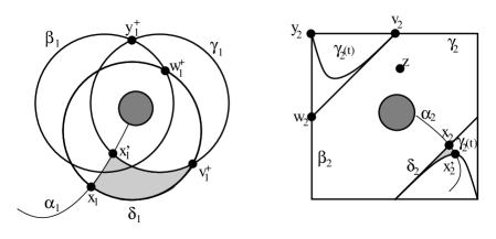
Figure 9. $+1$-surgery, $g=2$. The left side takes place in an annulus, the right side in a torus minus a disk; both are pieces of our genus two surface $\Sigma$ (the central disk missing from the annulus and the disk removed from the torus are both indicated by large grey circles). We have curves $\{\beta_{1},\beta_{2}\}$, $\{\gamma_{1},\gamma_{2}\}$ and $\{\delta_{1},\delta_{2}\}$ as in Lemma 9.2, with intersection points $\Theta_{\beta,\gamma}=\{y_{1}^{+},y_{2}\}$, $\Theta_{\gamma,\delta}=\{v_{1}^{+},v_{2}\}$, and $\Theta_{\beta,\delta}=\{w_{1}^{+},w_{2}\}$. The curve $\gamma_{2}(t)$ is isotopic to $\gamma_{2}$, but it approximates the juxtaposition of $\beta_{2}$ and $\delta_{2}$. We have also pictured arcs in $\alpha_{1}$ and $\alpha_{2}$. There is an intersection point $\mathbf{x}=\{x_{1},x_{2}\}$ for ${\mathbb{T}}_{\alpha}\cap{\mathbb{T}}_{\delta}$, and its nearest point ${\mathbb{T}}_{\alpha}\cap{\mathbb{T}}_{\gamma(t)}$, $\{x_{1}^{\prime},x_{2}^{\prime}\}=\rho(\mathbf{x})$. Observe the two lightly shaded triangles: they correspond to the canonical triangle in $\pi_{2}(\rho(\mathbf{x}),\Theta_{\gamma,\delta},\mathbf{x})$.

Proposition 9.7.

The map $f_{1}$ is chain homotopic to a $U$-equivariant chain map $g_{1}$ with the property that

$$\begin{CD}0@>{}>{}>CF^{+}(Y)@>{g_{1}}>{}>CF^{+}(Y_{0})@>{f_{2}}>{}>CF^{+}(Y_{1})@>{}>{}>0.\end{CD}$$

is a short exact sequence of chain complexes.

Theorem 9.1 is a consequence of this proposition: the associated long exact sequence is the exact sequence of Theorem 9.1.

For the construction of $g_{1}$, we need the following ingredients:

• lower-bounded filtrations on the $CF^{+}(Y)$, $CF^{+}(Y_{0})$, and $CF^{+}(Y_{1})$, which are strictly decreasing for the boundary maps; i.e. each chain complex is generated by elements with $\partial\xi<\xi$.

• an injection $\iota$ and splitting map $R$ as above, both of which respect the filtrations

• decompositions of $f_{1}=\iota+\text{lower order}$ and $f_{2}=\pi+\text{lower order}$, where, here, lower order is with respect to the filtrations. More precisely $CF^{+}(Y)$ is generated by elements $\xi$ with the property that $f_{1}(\xi)-\iota(\xi)<\iota(\xi)$, and $CF^{+}(Y_{1})$ is generated by elements $\eta$ with $\eta-f_{2}\circ R(\eta)<\eta$.

• $f_{2}\circ f_{1}$ is chain homotopic to zero by a $U$-equivariant homotopy

  $$H\colon CF^{+}(Y)\longrightarrow CF^{+}(Y_{1})$$

  which decreases filtrations, in the sense that $R\circ H<\iota$.

Following Lemma 9 of [4], we define a right inverse $R^{\prime}$ for $f_{2}$ by

$$R^{\prime}=R\circ\sum_{k=0}^{\infty}(\mathrm{Id}-f_{2}\circ R)^{\circ k},$$

and let

$$g_{1}=f_{1}-(\partial(R^{\prime}\circ H)+(R^{\prime}\circ H)\partial);$$

so that our hypotheses ensure that $g_{1}=\iota+{\text{lower order}}$. It follows that if $L$ is the left inverse of $\iota$ induced from $R$, then $L\circ g_{1}$ is invertible, as $L\circ g_{1}(\xi)=\xi-N(\xi)$, where $N$ decreases filtration (so we can define

$$(L\circ g_{1})^{-1}(\xi)=\sum_{k=0}^{\infty}N^{\circ k}(\xi),$$

as the sum on the right contains only finitely many non-zero terms for each $\xi\in CF^{+}(Y)$); thus, $(L\circ g_{1})^{-1}\circ L$ is a left inverse for $g_{1}$.

A similar argument shows surjectivity of $f_{2}$, and exactness at the middle stage (see [4]).

We will use a compatible energy filtration on $CF^{+}(Y_{0})$ defined presently. First, fix an $\mathbf{x}_{0}\in{\mathbb{T}}_{\alpha}\cap{\mathbb{T}}_{\beta}$. If $[\mathbf{y},j]\in CF^{+}(Y_{0})$, let $\psi\in\pi_{2}(\mathbf{x}_{0},\Theta_{\beta,\gamma},\mathbf{y})$ be a (homotopy class of) triangle, with $n_{z}(\psi)=-j$. We then define

$$\mathcal{F}_{Y_{0}}([\mathbf{y},j])=-\mathcal{A}(\psi).$$

(Note that $\pi_{2}(\mathbf{x}_{0},\Theta_{\beta,\gamma},\mathbf{y})$ is non-empty.) As in Lemma LABEL:HolDiskOne:lemma:EnergyZero of [27], the topological hypothesis from Lemma 9.2 allows us to use a volume form on $\Sigma$ for which every periodic domain for $Y_{0}$ has zero area: every periodic domain for $({\mathbb{T}}_{\beta},{\mathbb{T}}_{\delta})$, $({\mathbb{T}}_{\beta},{\mathbb{T}}_{\gamma(t)})$ and also the triply-periodic domain for $(\beta_{g},\gamma_{g}(t),\delta_{g})$ has area zero. (For example, we can start with the area form constructed in the proof of Lemma 9.2 for the initial $t=0$ $\gamma$-curves, and then move those curves by an exact Hamiltonian isotopy.) Now, the real-valued function $\mathcal{F}_{Y_{0}}$ on the generators of $CF^{+}(Y_{0})$ gives the latter group an obvious partial ordering.

We will assume now that the $\gamma_{g}(t)$ is sufficiently close to the juxtaposition of $\beta_{g}$ and $\delta_{g}$, in the following sense. Let $\mathcal{P}$ be a triply-periodic domain between $\gamma_{g}(t)$, $\beta_{g}$, and $\delta_{g}$ which generates the group of such periodic domains (this is the domain pictured in Figure 8, before $\gamma_{g}$ was isotoped); and for $i=1,...,g-1$, let $\mathcal{P}_{i}$ be the doubly-periodic domains with $\partial\mathcal{P}_{i}=\beta_{i}-\gamma_{i}(t)$. We let $\epsilon(t)$ be the sum of the absolute areas of all these periodic domains:

$$\epsilon(t)=\mathcal{A}\Big{(}|{\mathcal{D}}(\mathcal{P})|\Big{)}+\sum_{i=1}^{g-1}\mathcal{A}\Big{(}|{\mathcal{D}}(\mathcal{P}_{i})|\Big{)},$$

where here the absolute signs denote the unsigned area. Note that $\lim_{t\mapsto 0}\epsilon(t)=0$. Also, let $M$ be the minimum of the area of any domain in $\Sigma-\alpha_{1}-...-\alpha_{g}-\beta_{1}-...-\beta_{g}-\delta_{g}$. We choose $t$ small enough that $\epsilon(t)<M/2$. We assume that the absolute (unsigned) area of the periodic domain ${\mathcal{Q}}_{i}$ with $\partial({\mathcal{Q}}_{i})=\beta_{i}-\delta_{i}(t)$ agrees with the absolute area of ${\mathcal{P}}_{i}$.

Lemma 9.8.

For sufficiently small $t$, the function $\mathcal{F}_{Y_{0}}$ induces a filtration on $CF^{+}(Y_{0})$. In particular,

$$\partial[\mathbf{y},j]<[\mathbf{y},j].$$

Proof. It is important to observe that the area filtration defined above is indeed well-defined. The reason for this is that if $\psi,\psi^{\prime}$ are a pair of homotopy classes in $\pi_{2}(\mathbf{x}_{0},\Theta_{\beta,\gamma},\mathbf{y})$ with $n_{z}(\psi)=n_{z}(\psi^{\prime})$, then ${\mathcal{D}}(\psi)-{\mathcal{D}}(\psi^{\prime})$ is a triply-periodic domain. It follows from above that it must have total area zero.

Suppose that we have a pair of generators $[\mathbf{y},j]$ and $[\mathbf{y}^{\prime},j^{\prime}]$ which are connected by a flow $\phi$. If $\psi\in\pi_{2}(\mathbf{x}_{0},\Theta_{\beta,\gamma},\mathbf{y})$ is a class with $n_{z}(\psi)=-j$, then, of course, $\psi+\phi\in\pi_{2}(\mathbf{x}_{0},\Theta_{\beta,\gamma},\mathbf{y}^{\prime})$ is a class with $n_{z}(\psi+\phi)=-j^{\prime}$; thus, $\mathcal{F}_{Y_{0}}([\mathbf{y}^{\prime},j^{\prime}])-\mathcal{F}_{Y_{0}}([\mathbf{y},j])=-\mathcal{A}(\phi)$; but $\mathcal{A}(\phi)>0$, as all of its coefficients are non-negative (and at least one is positive).         

The filtration on $CF^{+}$, together with the data $\iota$, $\pi$, and $R$, endow $CF^{+}(Y)$ and $CF^{+}(Y_{1})$ with a filtration as well.

Lemma 9.9.

For $t$ sufficiently small, the orderings induced on $CF^{+}(Y)$ and $CF^{+}(Y_{1})$ give filtrations.

Proof. There is a natural filtration on $Y$, defined by $\mathcal{F}_{Y}([\mathbf{x},i])=-\mathcal{A}(\phi)$, where $\phi\in\pi_{2}(\mathbf{x}_{0},\mathbf{x})$ is the class with $n_{z}(\phi)=-i$. This is a filtration, in view of the usual positivity of holomorphic disks (see Lemma LABEL:HolDiskOne:lemma:NonNegativity); indeed, the filtration decreases by at least $M$ along flows.

The filtration induced by $\mathcal{F}_{Y_{0}}$ and the map $\iota$, defined by $\mathcal{F}_{Y}^{\prime}([\mathbf{x},i])=\mathcal{F}_{Y_{0}}(\iota[\mathbf{x},i])$ very nearly agrees with this natural filtration, for sufficiently small $t$. To see this, note that there is a unique “small” triangle $\psi_{0}\in\pi_{2}(\mathbf{x},\Theta_{\beta,\gamma},\iota(\mathbf{x}))$ which has non-negative coefficients and is supported inside the support of ${\mathcal{P}}+\mathcal{P}_{1}+...{\mathcal{P}}_{g-1}$. Clearly, $\mathcal{A}(\psi_{0})<\epsilon(t)$, and $n_{z}(\psi_{0})=0$. Now, if $\phi\in\pi_{2}(\mathbf{x}_{0},\mathbf{x})$ is the class with $n_{z}(\phi)=-i$ the juxtaposition of $\psi_{0}+\phi\in\pi_{2}(\mathbf{x}_{0},\Theta_{\beta,\gamma},\iota(\mathbf{x}))$ can be used to calculate the $Y_{0}$ filtration of $\iota(\mathbf{x})$; thus $|\mathcal{F}_{Y}([\mathbf{x},i])-\mathcal{F}_{Y}^{\prime}([\mathbf{x},i])|<\epsilon(t)$. In particular, since $\mathcal{F}_{Y}$ decreases by at least $M$ along flowlines, $\mathcal{F}_{Y_{0}}\circ\iota$, too, must decrease along flows.

For $Y_{1}$, there is another filtration, this one induced by squares. Given $[\mathbf{y},i]\in({\mathbb{T}}_{\alpha}\cap{\mathbb{T}}_{\delta})\times\mathbb{Z}^{\geq 0}$, consider $\varphi\in\pi_{2}(\mathbf{x}_{0},\Theta_{\beta,\gamma},\Theta_{\gamma,\delta},\mathbf{y})$ with $n_{z}(\varphi)=-i$, and let

$$\mathcal{F}_{Y_{1}}^{\prime\prime}([\mathbf{y},i])=-\mathcal{A}({\mathcal{D}}(\varphi)).$$

Indeed, if $M^{\prime}$ is the minimum area of any domain in $\Sigma-\alpha_{1}-...-\alpha_{g}-\delta_{1}(t)-...-\delta_{g-1}(t)-\delta_{g}$, then $\mathcal{F}_{Y_{1}}^{\prime\prime}$ decreases by at least $M^{\prime}$ along each flowline. Note that $M^{\prime}>M-\epsilon(t)$.

Now, we claim that $\mathcal{F}_{Y_{1}}^{\prime\prime}$ nearly agrees with the filtration $\mathcal{F}_{Y_{1}}^{\prime}$ induced by $\mathcal{F}_{Y_{0}}$ and the right inverse $R$: $\mathcal{F}_{Y_{1}}^{\prime}([\mathbf{y},j])=\mathcal{F}_{Y_{0}}(R[\mathbf{y},j])$. Again, if we let $\rho(\mathbf{y})$ denote the point in ${\mathbb{T}}_{\alpha}\cap\mathbb{T}\gamma(t)$ closest to $\mathbf{y}\in{\mathbb{T}}_{\alpha}\cap{\mathbb{T}}_{\delta}$, there is a unique small triangle $\psi_{0}\in\pi_{2}(\rho(\mathbf{y}),\Theta_{\gamma,\delta},\mathbf{y})$. If $\psi\in\pi_{2}(\mathbf{x}_{0},\Theta_{\beta,\gamma},\rho(\mathbf{y}))$ is a triangle with $n_{z}(\psi)=-j$ (i.e. used to calculate $\mathcal{F}_{Y_{0}}\circ R$), then, the juxtaposition $\psi+\psi_{0}$ is a square which can be used to calculate $\mathcal{F}_{Y_{1}}^{\prime\prime}([\mathbf{y},j])$. But $|\mathcal{A}(\psi+\psi_{0})-\mathcal{A}(\psi)|\leq\epsilon(t)$, so since $\mathcal{F}_{Y_{1}}^{\prime\prime}$ decreases by at least $M^{\prime}$ for non-trivial flows, it follows that $\mathcal{F}_{Y_{0}}\circ R$, too, must decrease along flows.         

Lemma 9.10.

The maps $f_{1}$ and $f_{2}$ have the form:

$$f_{1}=\iota+{\text{lower order}}, f_{2}|_{\mathrm{Im}R}=\pi+{\text{lower order}}$$

Proof. The map $f_{1}([\mathbf{x},i])$ counts the number of holomorphic triangles in homotopy classes with $\psi\in\pi_{2}(\mathbf{x},\Theta_{\beta,\gamma},\mathbf{y})$, with $\mathbf{y}\in{\mathbb{T}}_{\alpha}\cap{\mathbb{T}}_{\gamma(t)}$ and $\mu(\psi)=0$. One of these triangles, of course is the canonical small triangle $\psi_{0}\in\pi_{2}(\mathbf{x},\Theta_{\beta,\gamma},\iota(\mathbf{x}))$. One can calculate that $\#\mathcal{M}(\psi_{0})=1$. This gives the $\iota$ component of $f_{1}$. Now, no other homotopy class $\psi\in\pi_{2}(\mathbf{x},\Theta_{\beta,\gamma},\mathbf{y})$ with ${\mathcal{D}}(\psi)\geq 0$ has its domain ${\mathcal{D}}(\psi)$ contained inside the support of ${\mathcal{P}}+\mathcal{P}_{1}+...\mathcal{P}_{g-1}$; thus, if $\mathcal{M}(\psi)$ is non-empty, then $\mathcal{A}(\psi)>M-\epsilon(t)>M/2$. Moreover, in the proof of Lemma 9.9, we saw that if $\phi\in\pi_{2}(\mathbf{x}_{0},\mathbf{x})$ is the homotopy class with $n_{z}(\phi)=-i$, then

$$|\mathcal{F}_{Y_{0}}(\iota([\mathbf{x},i]))+\mathcal{A}(\phi)|<\epsilon(t).$$

But now $\psi+\phi$ can be used to calculate the filtration $\mathcal{F}_{Y_{0}}([\mathbf{y},i-n_{z}(\psi)])$. Thus,

$$\mathcal{F}_{Y_{0}}([\mathbf{y},i-n_{z}(\psi)])-\mathcal{F}_{Y_{0}}(\iota[\mathbf{x},i])\leq-\mathcal{A}(\psi)+\epsilon(t)<0.$$

Next, we consider $f_{2}$. As before, if $\mathbf{y}\in{\mathbb{T}}_{\alpha}\cap{\mathbb{T}}_{\delta}$, we let $\rho(\mathbf{y})\in{\mathbb{T}}_{\alpha}\cap{\mathbb{T}}_{\gamma(t)}$ denote the intersection point closest to $\mathbf{y}$. Suppose that $f_{2}([\rho(\mathbf{y}),i])$ has a non-zero component in $[\mathbf{w},j]$ with $[\mathbf{y},i]\neq[\mathbf{w},j]$; thus, we have a $\psi\in\pi_{2}(\rho(\mathbf{y}),\Theta_{\gamma,\delta},\mathbf{w})$ with $n_{z}(\psi)=i-j$, which supports a holomorphic triangle. Again, $\psi$ cannot be supported inside the support of ${\mathcal{P}}+\mathcal{P}_{1}+...+\mathcal{P}_{g-1}$, so $\mathcal{A}(\psi)>M/2$. Fix $\psi_{\mathbf{w}}\in\pi_{2}(\mathbf{x}_{0},\Theta_{\beta,\gamma},\rho(\mathbf{w}))$ (for ${\mathbb{T}}_{\alpha},{\mathbb{T}}_{\beta},{\mathbb{T}}_{\gamma}$) with $n_{z}(\psi_{\mathbf{w}})=-j$, and $\psi_{\mathbf{y}}\in\pi_{2}(\mathbf{x}_{0},\Theta_{\beta,\gamma},\rho(\mathbf{y}))$ with $n_{z}(\psi_{\mathbf{y}})=-i$. Clearly, the juxtaposition $\psi_{\mathbf{y}}+\psi\in\pi_{2}(\mathbf{x}_{0},\Theta_{\beta,\gamma},\Theta_{\gamma,\delta},\mathbf{w})$ is a square whose area must agree with the square $\psi_{\mathbf{w}}+\psi_{0}$, where $\psi_{0}\in\pi_{2}(\rho(\mathbf{w}),\Theta_{\gamma,\delta},\mathbf{w})$ is the canonical small triangle, so

$$\mathcal{A}(\psi_{\mathbf{w}})=\mathcal{A}(\psi_{\mathbf{y}})-\mathcal{A}(\psi_{0})+\mathcal{A}(\psi),$$

and hence $\mathcal{F}([\rho(\mathbf{y}),i])>\mathcal{F}([\rho(\mathbf{w}),j])$.         

Lemma 9.11.

For sufficiently small $t$, there is a null-homotopy $H$ of $f_{2}\circ f_{1}$ satisfying $R\circ H<\iota$.

Proof. Theorem LABEL:HolDiskOne:thm:Associativity of [27] provides the null-homotopy $H$: the $[\mathbf{y},j]$ coefficient of $H[\mathbf{x},i]$ counts holomorphic squares $\varphi\in\pi_{2}(\mathbf{x},\Theta_{\beta,\gamma},\Theta_{\gamma,\delta},\mathbf{y})$ with $n_{z}(\varphi)=i-j$.

Our aim here is to prove that if the $[\mathbf{y},j]$ component of $H[\mathbf{x},i]$ is non-zero then $\iota[\mathbf{x},i]>R[\mathbf{y},j]$. Now, the filtration difference between $\iota([\mathbf{x},i])$ and $R[\mathbf{y},j]$ is calculated (to within $\epsilon(t)$) by $\mathcal{A}(\psi)$, where $\psi\in\pi_{2}(\mathbf{x},\Theta_{\beta,\gamma},\rho(\mathbf{y}))$ has $n_{z}(\psi)=i-j$. Adding the smallest triangle in $\pi_{2}(\rho(\mathbf{y}),\Theta_{\gamma,\delta},\mathbf{y})$ (and hence changing the area by no more than $\epsilon(t)$), we obtain another square $\varphi^{\prime}\in\pi_{2}(\mathbf{x},\Theta_{\beta,\gamma},\Theta_{\gamma,\delta},\mathbf{y})$ with $n_{z}(\varphi^{\prime})=i-j$, whose area must agree with the area of $\varphi$. Now if $t$ is sufficiently small ($\epsilon(t)<M/4$), it follows that the filtration difference between $\iota[\mathbf{x},i]$ and $R[\mathbf{y},j]$ is positive.         

Proof of Theorem 9.1. Theorem 9.1 is now a consequence of the long exact sequence associated to the short exact sequence from Proposition 9.7, with a few final observations regarding the $\mathbb{Z}/{2}\mathbb{Z}$ grading.

Orient the $\alpha_{1},...,\alpha_{g}$, the $\beta_{1},...,\beta_{g-1}$ arbitrarily (hence inducing orientations on the $\gamma_{1},...,\gamma_{g-1}$ and the $\delta_{1},...,\delta_{g-1}$). The orientation on $\beta_{g}$ is then forced on us by the requirement that

$$1=\chi(\widehat{HF}(Y))=\#({\mathbb{T}}_{\alpha}\cap{\mathbb{T}}_{\beta}),$$

where we orient the tori ${\mathbb{T}}_{\alpha}$ and ${\mathbb{T}}_{\beta}$ in the obvious manner. Similarly, the orientation on $\delta_{g}$ is forced; indeed, so that

$$\delta_{g}=\beta_{g}\pm\gamma_{g}$$

We can orient $\gamma_{g}$ so that the above sign is positive. It is then clear with these conventions (by looking at the small triangles) that $F_{1}$ preserves the absolute $\mathbb{Z}/{2}\mathbb{Z}$ grading, while $F_{2}$ reverses it. It follows then that $F_{3}$ preserves degree as claimed.

∎

9.2. A generalization

Let $Y$ be an oriented three-manifold, and let $K\subset Y$ be a knot. Let $m$ be the meridian of $K$, and let $h\in H_{1}(\partial(Y-{\mathrm{nd}}(K)))$ be a homology class with $m\cdot h=1$ (here, the torus is oriented as the boundary of the neighborhood of $K$). We let $Y_{h}$ denote the three-manifold obtained by attaching a solid torus to $Y-{\mathrm{nd}}(K)$, with framing specified by $h$.

Fix a ${\mathrm{Spin}}^{c}$ structure $\mathfrak{s}_{0}$ over $Y-K$. We let

$$HF^{+}(Y_{h},[\mathfrak{s}_{0}])=\bigoplus_{\{\mathfrak{s}\big{|}\mathfrak{s}|_{Y-K}=\mathfrak{s}_{0}\}}HF^{+}(Y_{h},\mathfrak{s}).$$

We define $HF^{+}(Y,[\mathfrak{s}_{0}])$ similarly.

The following is a direct generalization of Theorem 9.1 (the case where $Y$ is an integer homology three-sphere, and $h$ is the “longitude” of $K$):

Theorem 9.12.

For each ${\mathrm{Spin}}^{c}$ structure $\mathfrak{s}_{0}$ on $Y-K$, we have the $U$-equivariant exact sequence:

$$\begin{CD}...@>{}>{}>HF^{+}(Y,[\mathfrak{s}_{0}])@>{}>{}>HF^{+}(Y_{h},[\mathfrak{s}_{0}])@>{}>{}>HF^{+}(Y_{h+m},[\mathfrak{s}_{0}])@>{}>{}>...\end{CD}$$

Corollary 9.13.

Let $Y$ be an integer homology three-sphere with a knot $K\subset Y$, and let $Y_{n}$ be the three-manifold obtained by $n$ surgery on $K$ where $n>0$, then there is a $U$-equivarant long exact sequence

$$\begin{CD}...@>{}>{}>HF^{+}(Y)@>{}>{}>HF^{+}(Y_{n})@>{}>{}>HF^{+}(Y_{n+1})@>{}>{}>...\end{CD}$$

The proof given in the previous section adapts to this context, after a few observations.

Note first that the map from $Y$ to $Y_{h}$ defined by counting triangles is naturally partitioned into equivalence classes. To see the decomposition agrees with what we have stated, we observe the following. Let $X$ be the pair-of-pants cobordism connecting $Y$, $Y_{h}$, and $\#^{g-1}(S^{2}\times S^{1})$. The four-manifold obtained by filling the last component with $\#^{g-1}(D^{3}\times S^{1})$ is the cobordism $W_{h}$ from $Y$ to $Y_{h}$ obtained by attaching a two-handle to $Y$ along $K$ with framing $h$.

Now, ${\mathrm{Spin}}^{c}$-equivalence classes of triangles for ${\mathbb{T}}_{\alpha}$, ${\mathbb{T}}_{\beta}$, ${\mathbb{T}}_{\gamma}$ agree with ${\mathrm{Spin}}^{c}$ structures on the cobordism $W_{h}$, since $\mathfrak{s}_{z}(\Theta_{\beta,\gamma})$ is a torsion ${\mathrm{Spin}}^{c}$ structure over $\#^{g-1}(S^{2}\times S^{1})$ (which extends uniquely over $\#^{g-1}(D^{3}\times S^{1})$). But two ${\mathrm{Spin}}^{c}$ structures on $Y$ and $Y_{h}$ extend over $W_{h}$ if and only if they agree on the knot complement $Y-K$ (thought of as a subset of both $Y$ and $Y_{h}$).

With this said, the maps $f_{1}$ and $f_{2}$ partition according to ${\mathrm{Spin}}^{c}$ structures on $Y-K$.

Next, we observe that there are in principle many periodic domains for the triple $({\mathbb{T}}_{\alpha},{\mathbb{T}}_{\beta},{\mathbb{T}}_{\gamma})$. By twisting normal to the $\alpha$, however, we can arrange that the triple is admissible. By choosing the volume form on $\Sigma$ appropriately, we can arrange that they all have zero signed area.

We can define the filtrations as before. Fix any $\mathbf{x}_{0}\in{\mathbb{T}}_{\alpha}\cap{\mathbb{T}}_{\beta}$ so that $\mathfrak{s}_{z}(\mathbf{x}_{0})$ restricts to $\mathfrak{s}_{0}$ on $Y-K$. The triangle connecting $\mathbf{x}_{0}$, $\Theta_{\beta,\gamma}$ and any intersection point $\mathbf{y}\in{\mathbb{T}}_{\alpha}\cap{\mathbb{T}}_{\gamma}$ with $\mathfrak{s}_{z}(\mathbf{y})|Y-K=\mathfrak{s}_{0}$ is guaranteed to exist, since the corresponding ${\mathrm{Spin}}^{c}$ structures extend over $W_{h}$. The area the of the domain of any such triangle can be used to define $\mathcal{F}_{Y_{h}}([\mathbf{y},i])$. The proof given before, then, applies.

9.3. Fractional Surgeries

There are other directions to generalize Theorem 9.1. We consider presently the case of fractional ($1/q$) surgeries on an integral homology three-sphere.

Let $Y$ be an integer homology three-sphere, and $K\subset Y$ be a knot. Let $Y_{0}$ be the manifold obtained by zero-surgery on $K$, and let $Y_{1/q}$ be obtained by $1/q$ surgery on $K$, where $q$ is a positive integer.

We fix a representation

$$H^{1}(Y;\mathbb{Z})\longrightarrow\mathbb{Z}/{q}\mathbb{Z}$$

taking generators to generators, and let

$$\underline{HF^{+}}(Y_{0},\mathbb{Z}/{q}\mathbb{Z})\cong\bigoplus_{\mathfrak{s}\in{\mathrm{Spin}}^{c}(Y_{0})}\underline{HF^{+}}(Y_{0},\mathfrak{s})$$

denote the corresponding homology group with twisted coefficient ring (in the sense of Section 8).

Theorem 9.14.

Let $Y$ be an integral homology three-sphere and let $q$ be a positive integer. Then, there is a $U$-equivariant exact sequence

$$\begin{CD}...@>{}>{}>\underline{HF^{+}}(Y_{0};\mathbb{Z}/{q}\mathbb{Z})@>{}>{}>HF^{+}(Y_{1/q})@>{}>{}>HF^{+}(Y)@>{}>{}>...\end{CD}$$

The proof of Lemma 9.2 in the present context gives us a generalized pointed Heegaard diagram $(\Sigma,\mbox{\boldmath$\alpha$},\mbox{\boldmath$\beta$},\mbox{\boldmath$\gamma$},\mbox{\boldmath$\delta$},z)$ with the property that:

• the Heegaard diagrams $(\Sigma,\mbox{\boldmath$\alpha$},\mbox{\boldmath$\beta$})$, $(\Sigma,\mbox{\boldmath$\alpha$},\mbox{\boldmath$\gamma$})$, and $(\Sigma,\mbox{\boldmath$\alpha$},\mbox{\boldmath$\delta$})$ describe $Y$, $Y_{0}$, and $Y_{1/q}$ respectively,

• for each $i=1,...,g-1$, the curves $\beta_{i}$, $\gamma_{i}$, and $\delta_{i}$ are small isotopic translates of one another, each pairwise intersecting in a pair of canceling transverse intersection points

• the curve $\delta_{g}$ is isotopic to the juxtaposition of $\beta_{g}$ with the $q$-fold juxtaposition of $\gamma_{g}$.

We can think concretely about $\underline{CF^{+}}(Y_{0};\mathbb{Z}/{q}\mathbb{Z})$ as follows. Let $\zeta=e^{\frac{2\pi i}{q}}$, and fix a reference point $\tau\in\gamma_{g}$, which we choose to be disjoint from all the other $\alpha$, $\beta$, and $\delta$. This gives rise to a codimension-one submanifold

$$V=\gamma_{1}\times...\times\times\gamma_{g-1}\times\{\tau\}\subset{\mathbb{T}}_{\gamma}.$$

Then, $\underline{CF^{+}}(Y_{0};\mathbb{Z}/{q}\mathbb{Z})$ is generated over $\mathbb{Z}$ by the basis $[\mathbf{x},i]\otimes\zeta^{j}$ where of course, $\mathbf{x}$ is an intersection point $\mathbf{x}\in{\mathbb{T}}_{\alpha}\cap{\mathbb{T}}_{\gamma}$ in the appropriate equivalence class, $i$ is a non-negative integer, and $j\in\mathbb{Z}/{q}\mathbb{Z}$. The boundary map then is given by

(11) $$\partial\left([\mathbf{x},i]\otimes\zeta^{j}\right)=\sum_{\mathbf{y}\in{\mathbb{T}}_{\alpha}\cap{\mathbb{T}}_{\gamma}}\sum_{\{\phi\in\pi_{2}(\mathbf{x},\mathbf{y})\big{|}\mu(\phi)=1\}}\left(\#\widehat{\mathcal{M}}(\phi)\right)\cdot[\mathbf{y},i-n_{z}(\phi)]\otimes\zeta^{j+\#(V\cap\partial_{\gamma}(\phi))}.$$

The quantity $V\cap\partial_{\gamma}(\phi)$ is the intersection number between the codimension-one submanifold $V\subset{\mathbb{T}}_{\gamma}$ with the path in ${\mathbb{T}}_{\gamma}$ obtained by restricting $\phi$ to the appropriate edge.

Again, we let $v_{g}$ be the intersection point between $\delta_{g}$ and $\gamma_{g}$. We now have $q$ different intersection points between $\delta_{g}$ and $\beta_{g}$, of which we choose one, labelled $w_{g}$, in the following Proposition 9.15. We will have no need for the $q-1$ other intersection points. Let $\Theta_{\beta,\gamma}$, $\Theta_{\gamma,\delta}$, and $\Theta_{\beta,\delta}$ be as before.

As in Proposition 9.3, if we let $\theta_{\beta,\delta}=[\Theta_{\beta,\delta},0]$, then $\theta_{\beta,\delta}$ is a cycle in $CF^{\infty}({\mathbb{T}}_{\beta},{\mathbb{T}}_{\delta})$. Note that the three-manifold described by the pair $(\Sigma,\mbox{\boldmath$\beta$},\mbox{\boldmath$\delta$})$ is now a sum $L(q,1)\#\left(\#_{i=1}^{g-1}(S^{1}\times S^{2})\right)$ (where $L(q,1)$ is a lens space).

Proposition 9.15.

For an appropriate choice $w_{g}\in\beta_{g}\cap\delta_{g}$ for $\beta_{g}$ with $\delta_{g}$, there are homotopy classes of triangles $\{\psi^{\pm}_{k}\}_{k=1}^{\infty}\in\pi_{2}(\Theta_{\beta,\gamma},\Theta_{\gamma,\delta},\Theta_{\beta,\delta})$ satisfying the following properties (for each $k$):

$$\mu(\psi^{\pm}_{k}) = 0,$$

$$n_{z}(\psi^{+}_{k}) = n_{z}(\psi^{-}_{k}),$$

$$n_{z}(\psi^{+}_{k}) < n_{z}(\psi^{+}_{k+1}),$$

Moreover, each triangle in $\pi_{2}(\Theta_{\beta,\gamma},\Theta_{\gamma,\delta},\Theta_{\beta,\delta})$ is ${\mathrm{Spin}}^{c}$ equivalent to some $\psi^{\pm}_{k}$. Also, the congruence class modulo $q$ of the intersection number $\#(V\cap\partial_{\gamma}(\psi))$ is independent of the choice of $\psi\in\pi_{2}(\Theta_{\beta,\gamma},\Theta_{\gamma,\delta},\Theta_{\beta,\delta})$. Furthermore, there is a choice of perturbations and complex structure with the property that for each $\Psi\in\pi_{2}(\mathbf{x},\Theta_{\gamma,\delta},\Theta_{\beta,\delta})$ (where $\mathbf{x}\in{\mathbb{T}}_{\beta}\cap{\mathbb{T}}_{\gamma}$) with $\mu(\Psi)=0$, we have that

$$\#\mathcal{M}(\Psi)=\left\{\begin{array}[]{ll}\pm 1&{\text{if $\Psi\in\{\psi^{\pm}_{k}\}_{k=1}^{\infty}$}}\\ 0&{\text{otherwise}}\end{array}\right..$$

Proof. The proof follows along the lines of Proposition 9.5. In this case, letting $\mathcal{P}$ be the generating periodic domain in the torus, we have that

$$\partial\mathcal{P}=\beta_{g}+q\gamma_{g}-\delta_{g}.$$

We must choose $w_{g}$ so that it is the $\beta_{g}$-$\delta_{g}$ corner point for the domain containing the basepoint $z$. Note that $\partial\mathcal{P}$ meets the reference point $\tau\in\gamma$ with multiplicity $q$. This proves the $q$ independence of the intersection number $\#(V\cap\partial_{\gamma}(\psi))$ of the choice of $\psi\in\pi_{2}(\Theta_{\beta,\gamma},\Theta_{\gamma,\delta},\Theta_{\beta,\delta})$. (See Figure 10.)

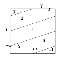
Figure 10. The triply-periodic domain in the torus relevant for $1/q$ surgery, with $q=3$.

    

Our choice of basepoint $z$ and the intersection point $\Theta_{\beta,\delta}$, from the above proposition give us a ${\mathrm{Spin}}^{c}$ structure $\mathfrak{t}_{\beta,\delta}\in{\mathrm{Spin}}^{c}(L(q,1)\#\left(\#_{i=1}^{g-1}(S^{1}\times S^{2})\right))$.

We consider the chain map

$$f_{2}\colon\underline{CF^{+}}(Y_{0},\mathbb{Z}/{q}\mathbb{Z})\longrightarrow CF^{+}(Y_{1/q})$$

defined by

$$f_{2}(\xi)=\sum_{\{\mathfrak{s}\in{\mathrm{Spin}}^{c}(X_{\alpha,\gamma,\delta})}\underline{f^{+}_{\alpha,\gamma,\delta}}(\xi\otimes\theta_{\gamma,\delta},\mathfrak{s}).$$

In the present context,

$$\underline{f^{+}_{\alpha,\gamma,\delta}}\left([\mathbf{x},i]\otimes\zeta^{k}\otimes[\mathbf{y},j];\mathfrak{s}\right)=\\ \sum_{\mathbf{w}\in{\mathbb{T}}_{\alpha}\cap{\mathbb{T}}_{\delta}}\sum_{\{\psi\in\pi_{2}(\mathbf{x},\mathbf{y},\mathbf{w})\big{|}\#(V\cap\partial_{\gamma}\psi)=-k,\mathfrak{s}_{z}(\psi)=\mathfrak{s}\}}\left(\#\mathcal{M}(\psi)\right)\cdot[\mathbf{w},i+j-n_{z}(\psi)].$$

We define

$$f_{3}\colon CF^{+}(Y_{1/q})\longrightarrow CF^{+}(Y)$$

by

$$f_{3}(\xi)=\sum_{\{\mathfrak{s}\in{\mathrm{Spin}}^{c}(X_{\alpha,\delta,\beta})\big{|}\mathfrak{s}|Y_{\beta,\delta}=\mathfrak{t}_{\beta,\delta}\}}f^{+}_{\alpha,\delta,\beta}(\xi\otimes\theta_{\beta,\delta},\mathfrak{s}).$$

This gives us maps:

$$\begin{CD}\underline{CF^{+}}(Y_{0},\mathbb{Z}/{q}\mathbb{Z})@>{f_{2}}>{}>CF^{+}(Y_{1/q})@>{f_{3}}>{}>CF^{+}(Y).\end{CD}$$

It follows, once again, from associativity, together with the Proposition 9.15 that the maps on homology $F_{3}\circ F_{2}=0$. Note that the chain homotopy evaluated on $\zeta^{k}\times[\mathbf{x},i]$ is constructed by counting squares in $\varphi\in\pi_{2}(\mathbf{x},\Theta_{\gamma,\delta},\Theta_{\delta,\beta},\mathbf{y})$ with $V\cap\partial_{\gamma}(\varphi)=-k$.

We homotope the $\delta$-curve to the juxtaposition of the $\beta_{g}$ with the $q$-fold juxtaposition of $\gamma_{g}$. This gives a short exact sequence of graded groups

$$\begin{CD}0@>{}>{}>\underline{CF^{+}}(Y_{0},\mathbb{Z}/{q}\mathbb{Z})@>{\iota}>{}>CF^{+}(Y_{1/q})@>{\pi}>{}>CF^{+}(Y)@>{}>{}>0.\end{CD}$$

To see the inclusion, note that each intersection point $\mathbf{x}$ of ${\mathbb{T}}_{\alpha}\cap{\mathbb{T}}_{\gamma}$ corresponds to $q$ distinct intersection points between ${\mathbb{T}}_{\alpha}\cap{\mathbb{T}}_{\delta}$, labelled $(\mathbf{x}_{1},...,\mathbf{x}_{q})$. For each of these intersection points, there is a unique smallest triangle $u_{1},...,u_{q}$, with $u_{i}\in\pi_{2}(\mathbf{x},,\Theta_{\gamma,\delta},\mathbf{x}_{j})$. We claim that the $q$ integers $\#(V\cap u_{i})$ each lie in different congruence classes modulo $q$. This gives the inclusion. To see surjection, note that each intersection point of $\mathbf{x}^{\prime}\in{\mathbb{T}}_{\alpha}\cap{\mathbb{T}}_{\beta}$ gives rise to a unique intersection point $\rho(\mathbf{x}^{\prime})$ between ${\mathbb{T}}_{\alpha}\cap{\mathbb{T}}_{\delta}$, which can be joined by a small triangle in $\pi_{2}(\rho(\mathbf{x}^{\prime}),\Theta_{\beta,\delta},\mathbf{x}^{\prime})$. (See Figure 11 for an illustration.)

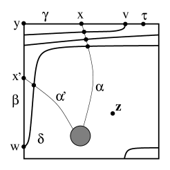
Figure 11. The analogue of Figure 9, only for $1/q$ surgery with $q=3$. We have pictured here only the part of the surface taking place in the final torus summand, and correspondingly dropped the $g$ subscripts. There are two $\alpha$-curves crossing the region here, labelled $\alpha$ and $\alpha^{\prime}$: the first of these meets $\gamma$ at $x$, the second meets $\beta$ at $x^{\prime}$. Observe the three intersection points of $\alpha\cap\delta$ and the intersection point of $\alpha^{\prime}\cap\delta$ corresponding to $x$ and $x^{\prime}$ respectively.

With this said, then, the energy filtration is defined as before, calculating the energy of classes $\psi\in\pi_{2}(\mathbf{x}_{0},\Theta_{\gamma,\delta},\mathbf{y})$. Thus we obtain the required long exact sequence.

9.4. $\widehat{HF}$

Let $Y$ be an oriented three-manifold, $K\subset Y$ be a knot, and $\mathfrak{s}_{0}$ be a fixed ${\mathrm{Spin}}^{c}$ structure over $Y-K$.

Theorem 9.16.

For each ${\mathrm{Spin}}^{c}$ structure $\mathfrak{s}_{0}$ on $Y-K$, we have the exact sequence:

$$\begin{CD}...@>{}>{}>\widehat{HF}(Y,[\mathfrak{s}_{0}])@>{}>{}>\widehat{HF}(Y_{h},[\mathfrak{s}_{0}])@>{}>{}>\widehat{HF}(Y_{h+m},[\mathfrak{s}_{0}])@>{}>{}>...\end{CD}$$

Similarly, we have:

Theorem 9.17.

Let $Y$ be an integral homology three-sphere and let $q$ be a positive integer. Then, there is a $U$-equivariant exact sequence

$$\begin{CD}...@>{}>{}>\underline{\widehat{HF}}(Y_{0};\mathbb{Z}/{q}\mathbb{Z})@>{}>{}>\widehat{HF}(Y_{1/q})@>{}>{}>\widehat{HF}(Y)@>{}>{}>...\end{CD}$$

For the proofs of these results, Proposition 9.15 (or Proposition 9.5, for the case of $+1$-surgeries) is replaced by the comparatively simpler:

Proposition 9.18.

There are two homotopy classes of triangles $\psi^{+}$ and $\psi^{-}$ in $\pi_{2}(\Theta_{\beta,\gamma},\Theta_{\gamma,\delta},\Theta_{\beta,\delta})$ with

$$\mu(\psi^{\pm}) = 0,$$

$$n_{z}(\psi^{\pm}) = 0,$$

$$\#(\partial_{\gamma}\psi^{+}) = \#(\partial_{\gamma}\psi^{-})+q.$$

Indeed, these are the only two triangles with ${\mathcal{D}}(\psi)\geq 0$ and $n_{z}(\psi)=0$. Also, each moduli space consists of a single, smooth isolated point.

Proof. This now follows directly from the picture in the torus. In particular, in the present case, there is no need for Theorem 9.4.         

Proof of Theorems 9.16 and 9.17. The proofs here are now obtained by copying the earlier proofs for $HF^{+}$, with the obvious notational changes. ∎

9.5. Integer surgeries

Another generalization of Theorem 9.1 involves integer surgeries.

Let $Y$ be an integer homology three-sphere, and $K\subset Y$ be a knot. Let $Y_{0}$ be the manifold obtained by zero-surgery on $K$, and let $Y_{p}$ be obtained by $+p$ surgery on $K$, where $p$ is a positive integer.

Theorem 9.19.

There is a surjective map $Q\colon{\mathrm{Spin}}^{c}(Y_{0})\longrightarrow{\mathrm{Spin}}^{c}(Y_{p})$ with the property that for each ${\mathrm{Spin}}^{c}$ structure $\mathfrak{t}\in{\mathrm{Spin}}^{c}(Y_{p})$, we have a $U$-equivariant exact sequence

$$\begin{CD}...@>{F_{1}}>{}>HF^{+}(Y_{0},[\mathfrak{t}])@>{F_{2}}>{}>HF^{+}(Y_{p},\mathfrak{t})@>{F_{3}}>{}>HF^{+}(Y)@>{}>{}>...,\end{CD}$$

where

$$HF^{+}(Y_{0},[\mathfrak{t}])=\bigoplus_{\{\mathfrak{t}_{0}\big{|}Q(\mathfrak{t}_{0})=\mathfrak{t}\}}HF^{+}(Y_{0},\mathfrak{t}_{0}).$$

Moreover, $F_{3}$ preserves $\mathbb{Z}/{2}\mathbb{Z}$ degree, chosen so that

$$\chi(\widehat{HF}(Y_{p},\mathfrak{t}))=\chi(\widehat{HF}(Y))=1.$$

In particular, there is a $U$-equivariant exact sequence

$$\begin{CD}...@>{}>{}>HF^{+}(Y_{0})@>{}>{}>HF^{+}(Y_{p})@>{}>{}>\bigoplus_{i=1}^{p}HF^{+}(Y)@>{}>{}>...,\end{CD}$$

Remark 9.20.

Indeed, a modification of the following proof can also be given to construct an exact sequence

$$\begin{CD}...@>{F_{2}}>{}>HF^{+}(Y)@>{F_{3}}>{}>HF^{+}(Y_{-p},\mathfrak{t})@>{F_{1}}>{}>HF^{+}(Y_{0},[\mathfrak{t}])@>{}>{}>...,\end{CD}$$

where $F_{3}$ preserves the $\mathbb{Z}/{2}\mathbb{Z}$ degree.

In another direction, Theorem 9.19 readily generalizes to the case where $Y$ is not an integral homology sphere. For example, if $K$ is a null-homologous knot in $Y$, there is still a notion of integral surgery, and we obtain sequences as above, only now there is one for each fixed ${\mathrm{Spin}}^{c}$ structure over $Y$.

Proof. This time, the curve $\delta_{g}$ is isotopic to the juxtaposition of the $p$-fold juxtaposition of $\beta_{g}$ with the $\gamma_{g}$.

Now, we have $p$ different intersection points between $\delta_{g}$ and $\gamma_{g}$. We choose one (so that the analogue of Proposition 9.15 holds, for our given choice of basepoint), and label it $v_{g}$. We will have no need for the remaining $p-1$ intersection points. Let $w_{g}$ denote the intersection point between $\beta_{g}$ and $\delta_{g}$, and let $\Theta_{\beta,\gamma}$, $\Theta_{\gamma,\delta}$, and $\Theta_{\beta,\delta}$ be as before. We have a corresponding ${\mathrm{Spin}}^{c}$ structure $\mathfrak{t}_{\gamma,\delta}$ corresponding to $\Theta_{\gamma,\delta}$.

If $\mathfrak{t}^{\prime}\in{\mathrm{Spin}}^{c}(Y_{0})$, there is a unique ${\mathrm{Spin}}^{c}$ structure $\mathfrak{t}\in{\mathrm{Spin}}^{c}(Y_{p})$ with the property that there is a ${\mathrm{Spin}}^{c}$ structure $\mathfrak{s}$ on $X_{\alpha,\gamma,\delta}$ with $\mathfrak{s}|Y_{0}=\mathfrak{t}^{\prime}$, $\mathfrak{s}|Y_{\gamma,\delta}=\mathfrak{t}_{\gamma,\delta}$, and $\mathfrak{s}|Y_{\alpha,\delta}=\mathfrak{t}$. We let $Q(\mathfrak{t}^{\prime})=\mathfrak{t}$.

Fix a ${\mathrm{Spin}}^{c}$ structure $\mathfrak{t}$ over $Y_{p}$. We consider the chain map

$$f_{2}\colon CF^{+}(Y_{0})\longrightarrow CF^{+}(Y_{p},\mathfrak{t})$$

defined by

$$f_{2}(\xi)=\sum_{\{\mathfrak{s}\in{\mathrm{Spin}}^{c}(X_{\alpha,\beta,\delta})\big{|}\mathfrak{s}|Y_{\alpha,\delta}=\mathfrak{t},~{}\mathfrak{s}|_{\gamma,\delta}=\mathfrak{t}_{\gamma,\delta}\}}f^{+}_{\alpha,\gamma,\delta}(\xi\otimes\theta_{\gamma,\delta},\mathfrak{s}).$$

We define $f_{3}$ as follows. Consider

$$f_{3}(\xi)=\sum_{\{\mathfrak{s}\in{\mathrm{Spin}}^{c}(X_{\alpha,\delta,\beta})\big{|}\mathfrak{s}|Y_{p}=\mathfrak{t}\}}f^{+}_{\alpha,\delta,\beta}(\xi\otimes\theta_{\beta,\delta}).$$

This gives us maps:

$$\begin{CD}CF^{+}(Y_{0},[\mathfrak{t}])@>{f_{2}}>{}>CF^{+}(Y_{p},\mathfrak{t})@>{f_{3}}>{}>CF^{+}(Y).\end{CD}$$

It follows once again from associativity, together with the analogue of Proposition 9.15, that $F_{3}\circ F_{2}=0$.

We homotope the $\delta$-curve to the juxtaposition of the $p$-fold multiple of $\beta_{g}$ with $\gamma_{g}$. This gives a short exact sequence of graded groups

$$\begin{CD}0@>{}>{}>CF^{+}(Y_{0},[\mathfrak{t}])@>{\iota}>{}>CF^{+}(Y_{p},\mathfrak{t})@>{\pi}>{}>CF^{+}(Y)@>{}>{}>0.\end{CD}$$

The inclusion follows as before: each intersection point $\mathbf{x}$ of ${\mathbb{T}}_{\alpha}\cap{\mathbb{T}}_{\gamma}$ corresponds a unique intersection point between ${\mathbb{T}}_{\alpha}\cap{\mathbb{T}}_{\delta}$, which can be canonically connected by a small triangle. To see surjection, note that each intersection point of $\mathbf{y}\in{\mathbb{T}}_{\alpha}\cap{\mathbb{T}}_{\beta}$ gives rise to $p$ different intersection points between ${\mathbb{T}}_{\alpha}\cap{\mathbb{T}}_{\delta}$, which we label $(\mathbf{y}_{1},...,\mathbf{y}_{p})$. Note, however, that $\epsilon(\mathbf{y}_{i},\mathbf{y}_{j})=(i-j)\mathrm{PD}[\beta_{g}^{*}]$. Now, $\mathrm{PD}[\beta_{g}^{*}]\in H^{2}(Y_{p})$ is a generator, so there will always be a unique induced intersection point representing the ${\mathrm{Spin}}^{c}$ structure $\mathfrak{t}$ over $Y_{p}$. The rest follows as before.         

9.6. $+1$ surgeries for twisted coefficients

There is also surgery exact sequence for $+1$ surgeries which uses twisted coefficients.

For simplicity, we state it in the case where we begin with a three-manifold $Y$ which is an integer homology sphere. In that case, if we let $T$ be a generator for $H^{1}(Y_{0};\mathbb{Z})$, then we can think of $\mathbb{Z}[H^{1}(Y_{0};\mathbb{Z})]$ as $\mathbb{Z}[T,T^{-1}]$. Given any $\mathbb{Z}[U]$ module $M$, let $M[T,T^{-1}]$ denote the induced module over $\mathbb{Z}[U,T,T^{-1}]$.

Theorem 9.21.

There is a $\mathbb{Z}[U,T,T^{-1}]$-equivariant long exact sequence:

$$\begin{CD}...@>{}>{}>HF^{+}(Y)[T,T^{-1}]@>{\underline{F^{+}_{1}}}>{}>\underline{HF^{+}}(Y_{0})@>{\underline{F^{+}_{2}}}>{}>HF^{+}(Y_{1})[T,T^{-1}]@>{\underline{F^{+}_{3}}}>{}>...\end{CD}$$

We will think of $\underline{HF^{+}}(Y_{0})$ like we did in Subsection 9.3: we fix a reference point $\tau\in\gamma_{g}$, and let the boundary map record, in the power of $T$, the multiplicity with which $\phi$ meets $\tau$ along its boundary, as in Equation (11) (with the difference that now we use a formal variable $T$ rather than a root of unity $\zeta$).

We will similarly use a reference point $\tau^{\prime}\in\delta_{g}$, again defining the boundary map for $Y_{1}$ which records the intersection with $\tau^{\prime}$ in the power of $T$, to obtain a chain complex for $Y_{1}$, which we write as: $CF^{+}(Y_{1},\mathbb{Z}[T,T^{-1}])$. Note that (by contrast with the case of $Y_{0}$) this has little effect on the homology. Indeed, it is easy to construct an isomorphism of chain complexes (over $\mathbb{Z}[U,T,T^{-1}]$):

$$CF^{+}(Y_{1})\otimes_{\mathbb{Z}}\mathbb{Z}[T,T^{-1}]\cong CF^{+}(Y_{1},\mathbb{Z}[T,T^{-1}]).$$

Moreover, it is clear that

$$H_{*}(CF^{+}(Y_{1})\otimes_{\mathbb{Z}}\mathbb{Z}[T,T^{-1}])\cong HF^{+}(Y_{1})\otimes_{\mathbb{Z}}\mathbb{Z}[T,T^{-1}].$$

However, this device will be convenient in constructing the chain maps.

We choose $\tau^{\prime}$ to lie on the boundary of $\psi^{-}$ and $\tau$ to lie on the boundary of $\psi^{+}$ (where $\psi^{\pm}=\psi^{\pm}_{1}$ from Proposition 9.5), and let $V$, $V^{\prime}$ be the corresponding codimension one subsets of ${\mathbb{T}}_{\gamma}$ and ${\mathbb{T}}_{\delta}$ respectively. We then let

$$\underline{f^{+}_{1}}([\mathbf{x},i])=\sum_{\mathbf{w}\in{\mathbb{T}}_{\alpha}\cap{\mathbb{T}}_{\gamma}}\sum_{\{\psi\in\pi_{2}(\mathbf{x},\Theta_{\beta,\gamma}.\mathbf{w})\big{|}\mu(\psi)=0\}}c(\mathbf{x},\mathbf{w},\psi)\cdot[\mathbf{w},i-n_{z}(\psi)],$$

and

$$\underline{f^{+}_{2}}([\mathbf{x},i])=\sum_{\mathbf{w}\in{\mathbb{T}}_{\alpha}\cap{\mathbb{T}}_{\delta}}\sum_{\{\psi\in\pi_{2}(\mathbf{x},\Theta_{\gamma,\delta},\mathbf{w})\big{|}\mu(\psi)=0\}}c(\mathbf{x},\mathbf{w},\psi)\cdot[\mathbf{w},i-n_{z}(\psi)];$$

where in both cases $c(\mathbf{x},\mathbf{w},\psi)\in\mathbb{Z}[T,T^{-1}]$ is given by

$$c(\mathbf{x},\mathbf{w},\psi)=(\#\mathcal{M}(\psi))\cdot\left(T^{\#(\partial_{\gamma}\psi\cap V)+\#(\partial_{\delta}\psi\cap V^{\prime})}\right).$$

We have the following analogue of Proposition 9.6:

Proposition 9.22.

The composition $\underline{F^{+}_{2}}\circ\underline{F^{+}_{1}}=0$.

Proof. Observe that for the homotopy classes $\{\psi^{\pm}_{k}\}_{k=1}^{\infty}$ from Proposition 9.5, we have that

$$\#(\partial_{\beta}\psi^{+}_{k}\cap V)+\#(\partial_{\delta}\psi^{+}_{k}\cap V^{\prime})=\#(\partial_{\beta}\psi^{-}_{k}\cap V)+\#(\partial_{\delta}\psi^{-}_{k}\cap V^{\prime})=1$$

This implies that the formal sum

$$\sum_{\mathfrak{s}_{\beta,\gamma,\delta}\in S_{\beta,\gamma,\delta}}\underline{f^{\leq 0}_{\beta,\gamma,\delta}}(\theta_{\beta,\gamma}\otimes\theta_{\gamma,\delta},\mathfrak{s}_{\beta,\gamma,\delta}) = \sum_{k=1}^{\infty}T\otimes\left(\left[\Theta_{\beta,\delta},-\frac{k(k-1)}{2}\right]-\left[\Theta_{\beta,\delta},-\frac{k(k-1)}{2}\right]\right)$$

$$= 0.$$

Thus, the proof follows from associativity as before.         

Proof of Theorem 9.21. With Proposition 9.22 replacing Proposition 9.6, the proof proceeds as the proof of Theorem 9.1. ∎

We have also the generalization for integer surgeries:

Theorem 9.23.

Let $Y$ be an integral homology three-sphere, let $K\subset Y$ be a knot in $Y$, and fix a positive integer $p$. For each ${\mathrm{Spin}}^{c}$ structure $\mathfrak{t}\in{\mathrm{Spin}}^{c}(Y_{p})$, we have a $\mathbb{Z}[U,T,T^{-1}]$-equivariant exact sequence

$$\begin{CD}...@>{F_{1}}>{}>\underline{HF^{+}}(Y_{0},[\mathfrak{t}])@>{F_{2}}>{}>HF^{+}(Y_{p},\mathfrak{t})[T,T^{-1}]@>{F_{3}}>{}>HF^{+}(Y)[T,T^{-1}]@>{}>{}>...,\end{CD}$$

where

$$\underline{HF^{+}}(Y_{0},[\mathfrak{t}])=\bigoplus_{\{\mathfrak{t}_{0}\big{|}Q(\mathfrak{t}_{0})=\mathfrak{t}\}}\underline{HF^{+}}(Y_{0},\mathfrak{t}_{0}),$$

using the map $Q\colon{\mathrm{Spin}}^{c}(Y_{0})\longrightarrow{\mathrm{Spin}}^{c}(Y_{p})$ be the map from Theorem 9.19.

Proof. Combine the refinements from Theorem 9.19 with those of Theorem 9.21.         

10. Calculation of $HF^{\infty}$

The main result of the present section is the complete calculation of $\underline{HF^{\infty}}(Y)$ purely in terms of the homological data of $Y$. We also give the following similar calculation of $HF^{\infty}(Y)$ when $b_{1}(Y)\leq 2$. We start with the latter construction, establishing the following:

Theorem 10.1.

Let $Y$ be a closed, oriented three-manifold with $b_{1}(Y)\leq 2$. Then, there is an equivalence class of orientation system over $Y$ with the following property. If $\mathfrak{s}_{0}$ is torsion, then

$$HF^{\infty}(Y;\mathfrak{s}_{0})\cong\mathbb{Z}[U,U^{-1}]\otimes_{\mathbb{Z}}\Lambda^{*}H^{1}(Y;\mathbb{Z})$$

as a $\mathbb{Z}[U]\otimes_{\mathbb{Z}}\Lambda^{*}(H_{1}(Y;\mathbb{Z})/\mathrm{Tors})$-module. Furthermore, if $\mathfrak{s}$ is not torsion,

$$HF^{\infty}(Y;\mathfrak{s})\cong\left(\mathbb{Z}[U]/{U^{n}-1}\right)\otimes_{\mathbb{Z}}\Lambda^{*}c_{1}(\mathfrak{s})^{\perp},$$

where $c_{1}(\mathfrak{s})^{\perp}\subset H^{1}(Y;\mathbb{Z})$ is the subgroup pairing trivially with $c_{1}(\mathfrak{s})$, and $n={\mathfrak{d}}(\mathfrak{s})/2$.

Remark 10.2.

Of course, in the above statement, we think of the usual cohomology $H^{1}(Y;\mathbb{Z})$ (with constant coefficients); but it will be apparent from the proof that for each choice of locally constant $\mathbb{Z}$ coefficient system, we obtain an orientation system for $HF^{\infty}$ for which the analogous isomorphism holds: this gives an identification between locally constant $\mathbb{Z}$ coefficient systems over $Y$ and equivalence classes of orientation system over $Y$.

The proof in some important special cases is given in Subsection 10.1, and the general case is proved in Subsection 10.2. We give also the “twisted” analogue in Subsection 10.3 which holds for arbitrary $b_{1}(Y)$.

The theorem describes the module structure of $HF^{+}(Y,\mathfrak{s}_{0})$ in sufficiently large degree, when $\mathfrak{s}_{0}$ is a torsion ${\mathrm{Spin}}^{c}$ structure and $b_{1}(Y)\leq 2$. It also allows us to pay off several other debts: first, it allows us to define an absolute $\mathbb{Z}/{2}\mathbb{Z}$ grading on the homology groups; then, combined with the discussion of Section 5, it allows us to relate $\chi(HF^{-}(Y,\mathfrak{s}))$ with Turaev’s torsion in Subsection 10.5 (though an alternative calculation could also be given by modifying directly the discussion in Section 5). It also allows us to extend the Euler characteristic calculations for $HF^{+}$ to the case where the ${\mathrm{Spin}}^{c}$ structure is torsion, c.f. Subsection 10.6. Finally, the result allows us to identify a “standard” orientation system for $Y$: the one for which Theorem 10.1 holds, with the usual $H^{1}(Y;\mathbb{Z})$ on the right-hand-side. (This justifies our practice of dropping the coefficient system from the notation for $HF^{\infty}$, and the other related groups.) Since the analogue of Theorem 10.1 in the twisted case (Theorem 10.12) holds without restriction on the Betti numbers of $Y$, it can be used to identify a canonical coherent system of orientations for any oriented three-manifold $Y$.

10.1. $HF^{\infty}(Y)$ when $H_{1}(Y;\mathbb{Z})=0$ or $\mathbb{Z}$

Theorem 10.3.

Theorem 10.1 holds when $Y$ is an integer homology three-sphere; i.e. over $\mathbb{Z}$, $HF^{\infty}(Y)$ is freely generated by generators $y_{i}$ for $i\in\mathbb{Z}$, with $Uy_{i}=y_{i-1}$.

Theorem 10.4.

Theorem 10.1 holds when the three-manifold in question $Y_{0}$ satisfies $H_{1}(Y_{0})\cong\mathbb{Z}$. More concretely, let $H\in H^{2}(Y_{0};\mathbb{Z})$ be a generator, and let $\mathfrak{s}_{0}$ denote the ${\mathrm{Spin}}^{c}$ structure with trivial first Chern class. Then if $\mathfrak{s}=\mathfrak{s}_{0}\pm n\cdot H$ with $n>0$, then $HF^{\infty}(Y_{0},\mathfrak{s})$ is freely generated by generators $x_{i}$ for $i\in 1,...,n$, with $Ux_{i}=x_{i-1}$, $Ux_{1}=x_{n}$. Moreover, $HF^{\infty}(Y_{0},\mathfrak{s}_{0})$ is freely generated by generators $x_{i}$, $y_{i}$ for $i\in\mathbb{Z}$, with $Uy_{i}=y_{i-1}$, $Ux_{i}=x_{i-1}$ and $\mathrm{gr}(x_{i},y_{i})=1$; also, $\mathrm{PD}[H]\cdot x_{i}=y_{i}$.

The main ingredient in the proof of the above results is the following:

Proposition 10.5.

Let $Y$ be an integer homology three-sphere, and $K\subset Y$ be a knot, then there is an identification:

$$HF^{\infty}(Y_{0},\mathfrak{s})\cong HF^{\infty}(Y,\mathfrak{s}_{0})/(U^{n}-1),$$

where $Y_{0}$ is the three-manifold obtained by zero-surgery on $K$, and where the divisibility of $c_{1}(\mathfrak{s})$ is $2n$.

This is proved in several steps.

We start with a Heegaard diagram $(\Sigma,\mbox{\boldmath$\alpha$},\mbox{\boldmath$\beta$},z)$ describing $Y_{0}$, with the property that $(\Sigma,\{\alpha_{2},...,\alpha_{g}\},\{\beta_{1},...,\beta_{g}\})$ describes the knot complement. Let $\gamma$ be a curve which intersects $\alpha_{1}$ once and is disjoint from $\{\alpha_{2},...,\alpha_{g}\}$, so that $(\Sigma,\{\gamma,\alpha_{2},...,\alpha_{g}\},\{\beta_{1},...,\beta_{g}\})$ represents $Y$. Indeed, we let $\gamma_{2},...,\gamma_{g}$ be small isotopic translates of $\alpha_{2},...\alpha_{g}$, with $\gamma_{i}\cap\alpha_{i}$ for $i=2,...,g$ consisting of a canceling pair of points $w^{\pm}_{i}$. Such a diagram can always be found (compare Lemma 9.2). We twist $\alpha_{1}$ along $\gamma$, and let $R^{\infty}(\mathfrak{s})$ resp. $L^{\infty}(\mathfrak{s})$ denote the subset of $CF^{\infty}(Y_{0},\mathfrak{s})$, generated by the $\gamma$-induced intersection points to the right resp. the left of the curve $\gamma$. Recall that if we twist sufficiently, then $L^{\infty}(\mathfrak{s})$ is a subcomplex (c.f. Proposition 5.6).

We relate $HF^{\infty}$ for $Y$ with $H_{*}(R^{\infty})$, as follows:

Lemma 10.6.

There is an isomorphism $H_{*}(R^{\infty})\cong HF^{\infty}(Y)$.

Proof. Let $\Theta_{\alpha,\gamma}\in{\mathbb{T}}_{\alpha}\cap{\mathbb{T}}_{\gamma}$ be the intersection point $\{\gamma\cap\alpha_{1},w_{2}^{+},...,w_{g}^{+}\}$. It follows as in the proof of Proposition 5.6 that there are no triangles $\psi\in\pi_{2}(\Theta_{\alpha,\gamma},\mathbf{x},\mathbf{y})$ with $\mathbf{x}\in L^{\infty}$, $\mathbf{y}\in{\mathbb{T}}_{\gamma}\cap{\mathbb{T}}_{\beta}$ and ${\mathcal{D}}(\psi)\geq 0$, and $\mu(\psi)=0$. Hence, counting holomorphic triangles whose ${\mathbb{T}}_{\alpha}\cap{\mathbb{T}}_{\gamma}$-vertex is $\Theta_{\alpha,\gamma}$, we obtain a map $H_{*}(R^{\infty})\longrightarrow HF^{\infty}(Y)$. On the chain level, this map has the form $\iota+{\text{lower order}}$, where $\iota[\mathbf{x},i]=[\mathbf{x}^{\prime},i-n_{z}(\psi_{\mathbf{x}})]$ where $\mathbf{x}^{\prime}$ is the intersection point on ${\mathbb{T}}_{\gamma}\cap{\mathbb{T}}_{\beta}$ closest to $x\in{\mathbb{T}}_{\alpha}\cap{\mathbb{T}}_{\beta}$, $\psi_{\mathbf{x}}$ is the unique small triangle (supported in the neighborhood of $\gamma$ and the support of the isotopies between $\gamma_{i}$ and $\alpha_{i}$ with non-negative multiplicities) and lower order is taken with respect to the energy filtration on $Y$. Moreover, there is a relative $\mathbb{Z}$-grading on both complexes, given by the Maslov index (where we take an “in” domain for $Y_{0}$). The map preserves this grading. Moreover, there are only finitely many generators in each degree. It follows then that the induced map is an isomorphism.         

We have seen that the map $H_{*}(R^{\infty})\longrightarrow H_{*}(L^{\infty})$ naturally splits into two pieces, $\delta_{1}$ and $\delta_{2}$, where $\delta_{1}$ uses the domains $\phi^{\mathrm{in}}$ from Lemma 5.5.

Lemma 10.7.

The map $\delta_{1}$ is an isomorphism.

Proof. This follows from the fact that on the chain level, $\delta_{1}$ has the form

$$\delta_{1}[\mathbf{x}^{+},i]=[\mathbf{x}^{-},i-n_{z}(\phi_{\mathbf{x}^{+},\mathbf{x}^{-}})]+\text{lower order}.$$

(Lemma 5.7), together with the fact that $\delta_{1}$ preserves the relative $\mathbb{Z}$ grading.         

Lemma 10.8.

The map $\delta_{2}$ is an isomorphism.

Proof. Fix an equivalence class of intersection points between ${\mathbb{T}}_{\alpha}\cap{\mathbb{T}}_{\beta}$, all of which are $\gamma$-induced. According to Section 5, if we wind sufficiently many times along $\gamma$ and move the basepoint $z$ sufficiently close to $\gamma$, then $\langle c_{1}(\mathfrak{s}),H\rangle$ can be made arbitrarily large. By moving the basepoint to change the ${\mathrm{Spin}}^{c}$ structure, we have that the complexes $L^{+}(\mathfrak{s})$ and $L^{+}(\mathfrak{s}^{\prime})$ (resp. $R^{+}(\mathfrak{s})$ and $R^{+}(\mathfrak{s}^{\prime})$) are identical. Moreover, if $\mathfrak{s}$ and $\mathfrak{s}^{\prime}$ are sufficiently positive, then the map $\delta_{2}^{+}$ is independent of the ${\mathrm{Spin}}^{c}$ structure.

Choose a degree $i$ sufficiently large that $H_{i}(R^{+})\cong H_{i}(R^{\infty})$ and $H_{i}(L^{+})\cong H_{i}(L^{\infty})$, and note under these identifications, the map induced on homology

$$\delta^{+}_{2}\colon H_{i}(R^{+})\longrightarrow H_{i-1}(L^{+})$$

agrees with $\delta_{2}$. For fixed $i$ and sufficiently large $\mathfrak{s}$, $\delta_{1}^{+}$ on $H_{i}(R^{+}(\mathfrak{s}))$ vanishes. Since $HF^{+}(Y,\mathfrak{s})$ is zero for all sufficiently large $\mathfrak{s}$, it follows from the long exact sequence induced from

$$\begin{CD}0@>{}>{}>L^{+}(\mathfrak{s})@>{}>{}>CF^{+}(Y,\mathfrak{s})@>{}>{}>R^{+}(\mathfrak{s})@>{}>{}>0\end{CD}$$

that $\delta=\delta^{+}_{1}+\delta^{+}_{2}\colon H_{*}(R^{+}(\mathfrak{s}))\longrightarrow H_{*}(L^{+}(\mathfrak{s}))$ is an isomorphism. It follows that the kernel of $\delta^{+}_{2}$ in degree $i$ is trivial. From this, it follows in turn that the kernel of $\delta^{+}_{2}$ is trivial in all larger degrees. Since $\delta_{1}^{+}$ decreases degree more than $\delta_{2}^{+}$, it is easy to see that the cokerenel of $\delta_{2}^{+}$ in dimension $i$ is trivial, as well. The lemma then follows.         

Proof of Proposition 10.5. Note that $\delta_{1}$ and and $\delta_{2}$ are both isomorphisms, and

$$\mathrm{gr}(\delta_{1}([\mathbf{x},i]),\delta_{2}([\mathbf{x},i]))=\pm 2n$$

for each generator $[\mathbf{x},i]$ for $CF^{+}(Y,\mathfrak{s})$. It follows that:

$$HF^{\infty}(Y_{0},\mathfrak{s})\cong H_{*}(R^{\infty})/(U^{n}-1).$$

Thus, the proposition follows from Lemma 10.6. ∎

Proof of Theorem 10.3. Since multiplication by $U$ is an isomorphism on $HF^{\infty}(Y,\mathfrak{s}_{0})$, Proposition 10.5 shows that $HF^{\infty}(Y)\cong HF^{\infty}(Y_{1})$, where $Y_{1}$ denotes the $+1$ surgery on any knot $K\subset Y$. Since any two integer homology three-spheres can be connected by sequences of $\pm 1$ surgeries, it follows that $HF^{\infty}(Y)\cong HF^{\infty}(S^{3})$, which we know has the claimed form. ∎

Proof of Theorem 10.4. This is a direct consequence of Theorem 10.3 and Proposition 10.5 when $c_{1}(\mathfrak{s})$ is non-torsion. In the torsion case, the induced maps on homology satisfy either $\delta_{1}=\delta_{2}$, or $\delta_{1}=-\delta_{2}$, according to the two possible orientation conventions for $Y$. The two possibilities give two different homology groups (over $\mathbb{Z}$). We define the standard orientation convention to be the one for which $\delta_{1}=-\delta_{2}$.

Finally, note that the action of $h\in H_{1}(Y_{0};\mathbb{Z})$ is given by $\pm\delta_{1}$, as can be easily seen from the geometric representative for the circle action (see Remark LABEL:HolDiskOne:rmk:GeoRep of [27]). ∎

10.2. The general case of Theorem 10.1

Definition 10.9.

Let $Z$ be a compact three-manifold with $\partial Z=T^{2}$. The kernel of the map

$$H_{1}(\partial Z)\longrightarrow H_{1}(Z)$$

is cyclic, generated by $d\ell$, where $\ell\subset T^{2}$ is a simple, closed curve. We call such a curve $\ell$ a longitude, and $d$ the divisibility of $Z$.

Proposition 10.10.

Suppose that $b_{1}(Z)=1$, and let $h_{1}$, $h_{2}$ be primitive homology classes in $H_{1}(T^{2};\mathbb{Z})$ and with $h_{1}\cdot\ell$ and $h_{2}\cdot\ell$ positive with $h_{1}\cdot h_{2}=1$. Then, if $HF^{\infty}$ of $Y_{h_{1}}$ and $Y_{h_{2}}$ satisfy the property Theorem 10.1, then so does $Y_{h_{1}+h_{2}}$.

Proof. Recall that the Floer homologies of a rational homology three-sphere have an absolute $\mathbb{Z}/{2}\mathbb{Z}$ grading, specified by

$$\chi(\widehat{HF}(Y))=|H_{1}(Y;\mathbb{Z})|.$$

From the exact sequence of Theorem 9.12, we have that

$$\begin{CD}..@>{}>{}>HF^{+}(Y_{h_{1}})@>{F_{1}}>{}>HF^{+}(Y_{h_{2}})@>{F_{2}}>{}>HF^{+}(Y_{h_{1}+h_{2}})@>{}>{}>...\end{CD}$$

The hypothesis in the sign guarantees that the degree shift occurs at $F_{1}$ (using the absolute $\mathbb{Z}/{2}\mathbb{Z}$ grading on each group). It follows that $HF^{\infty}(Y_{h_{1}+h_{2}})$ vanishes in all odd degrees. Indeed, since this is true when we take coefficients in $\mathbb{Z}/{p}\mathbb{Z}$ for all $p$; hence, $HF^{\infty}(Y_{h_{1}+h_{2}})$ has no torsion in even degrees. Since $\chi(HF^{\infty}(Y,\mathfrak{s})/(U-1))=1$ for all rational homology three-spheres, the result follows.         

Proposition 10.11.

Suppose that $Z$ be an oriented three-manifold with torus boundary. For each $h$ with the property that $h\cdot\ell=1$, we have an identification

$$HF^{\infty}(Y_{\ell},\mathfrak{s})\cong HF^{\infty}(Y_{h},\mathfrak{s}_{0})/(U^{n}-1)$$

where $\mathfrak{s}_{0}$ is a torsion ${\mathrm{Spin}}^{c}$ structure, $\mathfrak{s}_{0}|_{Z}=\mathfrak{s}|_{Z}$, and ${\mathfrak{d}}(\mathfrak{s})=2n$.

Proof. We adapt the proof of Proposition 10.5. We start with $(\Sigma,\{\alpha_{2},...,\alpha_{g}\},\{\beta_{1},...,\beta_{g}\})$ representing the knot complement $Z$, and then choose $\alpha_{1}$ to represent $\ell$ and $\gamma$ to represent $h$: i.e. $(\Sigma,\mbox{\boldmath$\alpha$},\mbox{\boldmath$\beta$})$ represents $Y_{\ell}$ and $(\Sigma,\{\gamma,\alpha_{2},...,\alpha_{g}\},\{\beta_{1},...,\beta_{g}\})$ represents $Y_{h}$. There is an added feature now, since the divisibility $d$ of $Z$ could be greater than one. It is still the case that for sufficiently large winding, all the intersection points are represented from $R^{\infty}(\mathfrak{s})$ or $L^{\infty}(\mathfrak{s})$, and, as in Lemma 5.5, all homotopy classes of maps $\phi$ with $\mu(\phi)=1$ admitting holomorphic representatives (connecting any two intersection points) satisfy that the property that $\partial_{\alpha}\phi$ uses the central point $p=\alpha_{1}\cap\gamma$ either once or zero times. Recall $\delta_{1}$ is the map defined using those homotopy classes which meet $p$ once. Now, there is a difference map

$$\eta\colon({\mathbb{T}}_{\alpha}\cap{\mathbb{T}}_{\beta})\times({\mathbb{T}}_{\alpha}\cap{\mathbb{T}}_{\beta})\longrightarrow\mathbb{Z}/{d}\mathbb{Z},$$

which is defined by

$$\eta(\mathbf{x},\mathbf{y})=\#\left(\partial_{\alpha_{1}}\phi\cap p\right)\pmod{d}.$$

There are corresponding splittings

$$L^{\infty}(\mathfrak{s})=L^{\infty}_{1},...,L^{\infty}_{d} R^{\infty}(\mathfrak{s})=R^{\infty}_{1},...,R^{\infty}_{d}.$$ and

labeled so that $\eta(\mathbf{x},\mathbf{y})=1$ if $\mathbf{x}\in R^{\infty}_{i}$ and $\mathbf{y}\in R^{\infty}_{i+1}$, and $\delta_{1}(R^{\infty}_{i})\subset L^{\infty}_{i+1}$. and $\delta_{2}(R^{\infty}_{i})\subset L^{\infty}_{i}$.

The proof of Lemma 10.6 gives us that $H_{*}(R^{\infty}_{i})\cong HF^{\infty}(Y,\mathfrak{s}_{0})$ (for $i=1,...,d$). Also, analogues of Lemmas 10.7 and 10.8 still hold: both $\delta_{1}$ and $\delta_{2}$ are isomorphisms. Now, the proposition easily follows as before.         

Proof of Theorem 10.1. We begin with the case where $b_{1}(Y)=0$, and prove the claim by induction on $|H_{1}(Y;\mathbb{Z})|$. The base case is, of course, Theorem 10.3. For the inductive step, we choose a knot $K\subset Y$ which represents a non-trivial homology class. With appropriate orientation, we have that $m\cdot\ell>0$. If $m\cdot\ell>1$, the inductive step follows from Proposition 10.10, since $m$ can be decomposed as $m=h_{1}+h_{2}$ with $h_{1}\cdot h_{2}=1$, $h_{1}\cdot\ell,h_{2}\cdot\ell>1$. Note also that if $h\cdot\ell>0$, then $|H_{1}(Y_{h})|$ depends linearly on $h\cdot\ell$.

If $m\cdot\ell=1$, then since $K$ is homologically non-trivial, we must have that $d>1$. Also, $|\mathrm{Tors}H_{1}(Y_{\ell})|=\frac{1}{d}|\mathrm{Tors}H_{1}(Y)|$. Applying Proposition 10.11 along a different knot in $Y_{\ell}$ which represents a generator for $H_{1}(Y_{\ell})/\mathrm{Tors}$, we see that

$$HF^{\infty}(Y_{\ell},\mathfrak{s})\cong HF^{\infty}(Y^{\prime},\mathfrak{s}^{\prime})/(U^{n}-1),$$

where $|H_{1}(Y^{\prime};\mathbb{Z})|<|H_{1}(Y;\mathbb{Z})|$. Applying the proposition again, and the induction hypothesis, we obtain that $HF^{\infty}(Y)\cong\mathbb{Z}[U,U^{-1}]$.

The proof for general $b_{1}(Y)=1$ or $2$ follows from an induction on $b_{1}(Y)$. Let $Y$ be an oriented three-manifold with $b_{1}(Y)=1$ or $2$. Choose a knot $K\subset Y$ whose image in $H_{1}(Y;\mathbb{Z})/\mathrm{Tors}$ is primitive. (This implies that in $Y-K$, the divisibility $d=1$.) If $\mathfrak{s}$ is a non-torsion ${\mathrm{Spin}}^{c}$ structure on $Y_{\ell}$, then the result follows from Proposition 10.11. The other case follows from the fact that we have two maps $\delta_{1}$ and $\delta_{2}$ from $R^{\infty}(\mathfrak{s})$ to $L^{\infty}(\mathfrak{s})$, and both of these maps are isomorphisms of $\mathbb{Z}[U]\otimes_{\mathbb{Z}}\Lambda^{*}\left(H_{1}(Y_{h};\mathbb{Z})/\mathrm{Tors}\right)$-modules (between two modules are, in turn, isomorphic to $\mathbb{Z}[U^{-1}]\otimes_{\mathbb{Z}}\Lambda^{*}H^{1}(Y_{h};\mathbb{Z})$). Now, observe that the automorphism of $\mathbb{Z}[U]\otimes_{\mathbb{Z}}\Lambda^{*}\left(H_{1}(Y_{h};\mathbb{Z})/\mathrm{Tors}\right)$-module $\mathbb{Z}[U]\otimes_{\mathbb{Z}}\Lambda^{*}\left(H_{1}(Y_{h};\mathbb{Z})/\mathrm{Tors}\right)$ is determined by its action on the determinant line $\Lambda^{b}(H_{1}(Y_{h};\mathbb{Z})/\mathrm{Tors})\cong\mathbb{Z}$, where it is either multiplication by $+1$ or $-1$. Thus, the maps $\delta_{1}$ and $\delta_{2}$ either cancel (for one orientation convention) or they do not (for the other one). The convention where $\delta_{1}+\delta_{2}=0$ is the one for which the theorem follows; it is, in this case, the standard orientation convention for $Y$. ∎

10.3. The twisted case

We state a version of Theorem 10.1 which holds for arbitrary first Betti number.

Observe that the proof of Theorem 10.1 breaks down when $b_{1}(Y)\geq 3$, since now the module $\mathbb{Z}[U]\otimes_{\mathbb{Z}}\Lambda^{*}(\mathbb{Z}^{b-1})$ has non-trivial automorphisms, so that $\delta_{1}$ and $\delta_{2}$ do not necessarily cancel. Indeed, it is proved in [31] that

$$HF^{\infty}(T^{3},\mathfrak{s}_{0})\cong\mathbb{Z}[U,U^{-1}]\otimes_{\mathbb{Z}}\Big{(}H^{1}(T^{3})\oplus H^{2}(T^{3})\Big{)}$$

where $\mathfrak{s}_{0}$ is the ${\mathrm{Spin}}^{c}$ structure with $c_{1}(\mathfrak{s}_{0})=0$.

There is, however, a version which holds for twisted coefficient systems.

Observe first that the twisted homology group $\underline{HF^{\infty}}(Y,\mathfrak{s})$ is a module over the group-ring $\mathbb{Z}[H^{1}(Y;\mathbb{Z})]\otimes_{\mathbb{Z}}\mathbb{Z}[U,U^{-1}]$ (which can be thought of as a ring of Laurent polynomials in $b_{1}(Y)+1$ variables). To make the ring structure respect the relative grading, we give $\underline{HF^{\infty}}(Y,\mathfrak{s}_{0})$ a relative $\mathbb{Z}/{2}\mathbb{Z}$ grading.

Theorem 10.12.

Let $Y$ be a closed, oriented three-manifold. Then, there is a unique equivalence class of orientation system for which we have a $\mathbb{Z}[U,U^{-1}]\otimes_{\mathbb{Z}}\mathbb{Z}[H^{1}(Y;\mathbb{Z})]$-module isomorphism for each torsion ${\mathrm{Spin}}^{c}$ structure $\mathfrak{s}_{0}$ on $Y$:

$$\underline{HF^{\infty}}(Y,\mathfrak{s}_{0})\cong\mathbb{Z}[U,U^{-1}],$$

where here the latter group is endowed with a trivial action by $H^{1}(Y;\mathbb{Z})$.

Proof. The proof is obtained by modifying the above proof of Theorem 10.1, with minor modifications, which we outline presently.

For the case where $H_{1}(Y_{0};\mathbb{Z})\cong\mathbb{Z}$, we adapt the proof of Theorem 10.4, thinking of $\mathbb{Z}[H^{1}(Y;\mathbb{Z})]$ as $\mathbb{Z}[T,T^{-1}]$. In this case, Lemma 10.6 is replaced by an isomorphism $H_{*}(R^{\infty})\cong HF^{\infty}(Y)[T,T^{-1}]$ (with the same proof). Next, we observe that rather than having $\delta_{1}$ and $\delta_{2}$ cancel, as in the proof of Theorem 10.4, we have that $\delta_{1}=\pm\delta_{2}\cdot T$. In fact, for some choice of orientation convention, we can arrange for $\delta_{1}=-\delta_{2}$. The result then follows easily from the long exact sequence connecting ${\underline{L}}^{\infty}(Y,\mathfrak{s})$, $\underline{HF^{\infty}}(Y,\mathfrak{s})$, and ${\underline{R}}^{\infty}(\mathfrak{s})$ observing that the map

$$\mathbb{Z}[T,T^{-1}]\stackrel{{\scriptstyle 1-T}}{{\longrightarrow}}\mathbb{Z}[T,T^{-1}]$$

injective, with cokernel $\mathbb{Z}$ (with trivial action by $T$).

The same modifications work to prove the general case (arbitrary $b_{1}(Y)$) as well.

We now turn to the uniqueness assertion on the orientation system. For the various equivalence classes of orientation systems, it is always true that $\underline{HF^{\infty}}(Y,\mathfrak{s}_{0})\cong\mathbb{Z}[U,U^{-1}]$ as a $\mathbb{Z}$ module. In fact, we saw (c.f. Equation (9)) that as a $\mathbb{Z}$ module, the isomorphism class of the chain complex $\underline{CF^{\infty}}(Y,\mathfrak{s}_{0})$ is independent of the choice of orientation system. Moreover, from Equation (9), it is clear that the $2^{b_{1}(Y)}$ different equivalence classes of coherent orientation system give rise to all $2^{b_{1}(Y)}$ different $\mathbb{Z}[H^{1}(Y;\mathbb{Z})]$-module structures on $\mathbb{Z}[U,U^{-1}]$ which correspond naturally to $\mathrm{Hom}(H^{1}(Y;\mathbb{Z}),\mathbb{Z}/{2}\mathbb{Z})$, with a distinguished module for which the action by $H^{1}(Y;\mathbb{Z})$ is trivial.         

Remark 10.13.

In fact, the above argument shows in general that for any ${\mathrm{Spin}}^{c}$ structure over $Y$, there is an identification of $\mathbb{Z}[U,U^{-1}]$ modules $\underline{HF^{\infty}}(Y,\mathfrak{s}_{0})\cong\mathbb{Z}[U,U^{-1}]$. However, the action of $\xi\in H^{1}(Y;\mathbb{Z})$ will, in general, be given by multiplication by $U^{k}$, where $k$ is given by $2k=\langle\xi\cup c_{1}(\mathfrak{s}),[Y]\rangle$.

10.4. Absolute $\mathbb{Z}/{2}\mathbb{Z}$ gradings

With the help of Theorem 10.12, we can define an absolute $\mathbb{Z}/{2}\mathbb{Z}$ grading on $CF^{\infty}(Y,\mathfrak{s})$ (and hence all the other associated chain complexes), for all ${\mathrm{Spin}}^{c}$ structures, simultaneously.

We declare the non-zero generators of $\underline{HF^{\infty}}(Y,\mathfrak{s})$ to have even degree. Note that for a rational homology three-sphere, this orientation convention agrees with that used before, i.e. $\chi(\widehat{HF}(Y))=|H_{1}(Y;\mathbb{Z})|$. (In fact, if we orient ${\mathbb{T}}_{\alpha}$ and ${\mathbb{T}}_{\beta}$ so that the intersection number $\#({\mathbb{T}}_{\alpha}\cap{\mathbb{T}}_{\beta})=|H_{1}(Y;\mathbb{Z})|$, then the $\mathbb{Z}/{2}\mathbb{Z}$ grading at a generator $[\mathbf{x},i]$ is $+1$ if and only if the local intersection number of ${\mathbb{T}}_{\alpha}$ and ${\mathbb{T}}_{\beta}$ at $\mathbf{x}$ is $+1$.)

With this orientation convention, we have the following refinement of Corollary 1.3:

Proposition 10.14.

Let $Y_{0}$ be an oriented three-manifold with $b_{1}(Y_{0})=1$, and $\mathfrak{s}$ be a non-torsion ${\mathrm{Spin}}^{c}$ structure, then

$$\chi(HF^{+}(Y_{0},\mathfrak{s}_{0}+nH))=-\tau_{t}(Y_{0},\mathfrak{s}),$$

where $t$ is the component containing $c_{1}(\mathfrak{s})$, and the sign on $\tau_{t}(Y_{0},\mathfrak{s})$ is specified by

$$\tau_{-t}(\mathfrak{s})-\tau_{t}(\mathfrak{s})=n.$$

In particular, if $Y_{0}$ is obtained by zero-surgery on a knot $K$ in a homology three-sphere, whose symmetrized Alexander polynomial is

$$\Delta_{K}=a_{0}+\sum_{i=1}^{d}a_{i}(T^{i}+T^{-i}),$$

then

$$\chi(HF^{+}(Y_{0},\mathfrak{s}_{0}+nH)=-\sum_{j=1}^{d}ja_{|n|+j}.$$

Proof. First observe that the sign comparing $\chi(HF^{+}(Y_{0}))$ and $\tau_{t}$ in Theorem 5.2 is universal, depending on the relative sign between $\Delta_{i,j}$ and $\Delta^{\prime}_{i,j}$. Checking these signs for $S^{1}\times S^{2}$, the Proposition follows.         

10.5. The Euler characteristic of $HF^{-}$

The following is an immediate consequence of Theorem 5.2, together with Theorem 10.4 (though a more direct proof can be given by modifying the discussion in Section 5):

Corollary 10.15.

Let $Y$ be an oriented three-manifold with $b_{1}(Y)=1$, and $\mathfrak{s}\in{\mathrm{Spin}}^{c}(Y)$ be a non-torsion ${\mathrm{Spin}}^{c}$ structure. Then, $\chi(HF^{-}(Y,\mathfrak{s}))=\tau_{-t}(\mathfrak{s})$, where $t$ is the component of $H^{2}(Y;\mathbb{Z})-0$ containing $c_{1}(\mathfrak{s})$

Proof. The short exact sequence

$$\begin{CD}0@>{}>{}>CF^{-}(Y,\mathfrak{s})@>{}>{}>CF^{\infty}(Y,\mathfrak{s})@>{}>{}>CF^{+}(Y,\mathfrak{s})@>{}>{}>0.\end{CD}$$

induced a long exact sequence in homology

$$\begin{CD}@>{}>{}>HF^{-}(Y,\mathfrak{s})@>{}>{}>HF^{\infty}(Y,\mathfrak{s})@>{}>{}>HF^{+}(Y,\mathfrak{s})@>{}>{}>...,\end{CD}$$

which shows that

$$\chi(HF^{\infty}(Y,\mathfrak{s}))=\chi(HF^{+}(Y,\mathfrak{s}))+\chi(HF^{-}(Y,\mathfrak{s})).$$

Moreover, Theorem 10.1 implies that

$$\chi(HF^{\infty}(Y,\mathfrak{s}))=n,$$

where $2n$ is the divisibility of $c_{1}(\mathfrak{s})$ in $H^{2}(Y,\mathfrak{s})/\mathrm{Tors}$. The result now follows from the “wall-crossing formula”:

$$\tau_{-t}(Y,\mathfrak{s})-\tau_{t}(Y,\mathfrak{s})=n$$

for Turaev’s torsion (see [36]).         

Corollary 10.16.

If $Y$ is an oriented three-manifold with $b_{1}(Y)=1$ or $2$ and $\mathfrak{s}\in{\mathrm{Spin}}^{c}(Y)$ is a non-torsion ${\mathrm{Spin}}^{c}$ structure, then $\chi\left(HF^{-}(Y,\mathfrak{s})\right)=\pm\tau(\mathfrak{s})$.

Proof. This follows in the same manner as the previous corollary, except that now $c_{1}(\mathfrak{s})^{\perp}$ is a non-trivial vector space, so its exterior algebra has Euler characteristic zero: thus, $\chi(HF^{\infty}(Y,\mathfrak{s}))=0$.         

10.6. The truncated Euler characteristic

In Theorem 5.2, we worked with a non-torsion ${\mathrm{Spin}}^{c}$ structure. The reason for this, of course, is given Theorem 10.1: if $\mathfrak{s}_{0}$ is torsion and $Y_{0}$ is a three manifold with $0<b_{1}(Y)=b\leq 2$, then in all sufficiently large degrees $i$, $HF^{+}_{i}(Y_{0},\mathfrak{s}_{0})\cong HF^{\infty}_{i}(Y_{0},\mathfrak{s}_{0})\cong\mathbb{Z}^{2^{b_{1}(Y)-1}}$. This shows, however, that for all sufficiently large $n$, the Euler characteristic of the graded Abelian group $HF^{+}_{\leq n}(Y_{0},\mathfrak{s}_{0})$ takes on two possible values, depending on the parity of $n$ (and the difference between the two values is $2^{b_{1}(Y)-1}$). In fact, we have the following:

Theorem 10.17.

Let $Y$ be a three-manifold with $b_{1}(Y)=1$ or $2$, equipped with a torsion ${\mathrm{Spin}}^{c}$ structure $\mathfrak{s}_{0}$. Then, when $b_{1}(Y)=1$, then for all sufficiently large $n$

$$\chi(HF^{+}_{\leq n}(Y,\mathfrak{s}_{0}))=\left\{\begin{array}[]{ll}-\tau(Y)&{\text{for odd $n$}}\\ -\tau(Y)+1&{\text{for even $n$}}\end{array}\right.$$

When $b_{1}(Y)=2$, then in all sufficiently large degrees,

$$\chi(HF^{+}_{\leq n}(Y,\mathfrak{s}_{0}))=\pm\tau(Y)+(-1)^{n}.$$

Proof. As before, we have a short exact sequence

$$\begin{CD}0@>{}>{}>L^{+}@>{}>{}>CF^{+}(Y_{0},\mathfrak{s}_{0})@>{}>{}>R^{+}@>{}>{}>0,\end{CD}$$

and hence a long exact sequence:

$$\begin{CD}...@>{}>{}>H_{i}(L^{+})@>{}>{}>HF^{+}_{i}(Y,\mathfrak{s}_{0})@>{}>{}>H_{i}(R^{+})@>{\delta}>{}>...\end{CD}$$

Note that we are using a relative $\mathbb{Z}$ grading here, which we can do since $\mathfrak{s}_{0}$ is torsion. When $i$ is sufficiently large, the coboundary map $\delta$ is zero, since on $HF^{\infty}$, the map $H_{*}(L^{\infty})\longrightarrow HF^{\infty}(Y)$ is an injection.

It follows that for all sufficiently large $n$,

(12) $$\chi(HF^{+}_{\leq n}(Y))=\chi(H_{\leq n}(L^{+}))+\chi(H_{\leq n}(R^{+})).$$

On the other hand, we still have a short exact sequence:

$$\begin{CD}0@>{}>{}>{\ker f_{1}}@>{}>{}>R^{+}@>{f_{1}}>{}>L^{+}@>{}>{}>0,\end{CD}$$

inducing

$$\begin{CD}@>{}>{}>H_{i}({\ker f_{1}})@>{}>{}>H_{i}(R^{+})@>{f_{1}}>{}>H_{i-1}(L^{+})@>{}>{}>...\end{CD}$$

Note that with the earlier grading conventions, $f_{1}$ must decrease the grading by one. Of course, $\ker f_{1}$ is a finite-dimensional graded vector space, so the above gives the following relation for all sufficiently large $n$:

(13) $$\chi({\ker f_{1}})=\chi(H_{\leq n}(R^{+}))+\chi(H_{\leq n-1}(L^{+})).$$

But from Proposition 5.10 applies in the present case, to identify $\chi({\ker f_{1}})=\tau(\mathfrak{s}_{0})$. Note that the proof of the that proposition does not really require that $\mathfrak{s}$ be negative; it suffices to consider the case where $\mathfrak{s}+\alpha_{1}^{*}$, $\mathfrak{s}+\beta_{j}^{*}$ and $\mathfrak{s}+\alpha_{1}^{*}+\beta_{j}^{*}$ are negative, and $c_{1}(\mathfrak{s})$ is torsion. Combining this result, Equation (12), and Equation (13), we obtain that:

$$\chi(HF^{+}_{\leq n}(Y,\mathfrak{s}_{0}))=-\tau(Y,\mathfrak{s}_{0})+(-1)^{n}\mathrm{rk}H_{n}(L^{+},\mathfrak{s}_{0}).$$

Suppose that $b_{1}(Y)=1$. Then, (according to Theorem 10.1) for all sufficiently large $n$, $\mathrm{rk}H_{n}(L^{+},\mathfrak{s}_{0})=1$ if $n$ is even and $0$ when $n$ is odd. Similarly, when $b_{1}(Y)=2$, we have

$$\mathrm{rk}H_{n}(L^{+},\mathfrak{s}_{0})=\mathrm{rk}HF^{\infty}_{n}(Y)/2=1.$$

    

10.7. On the role of $n_{z}$

The “triviality” of $HF^{\infty}(Y)$ – its dependence on the homological information of $Y$ alone – underscores the importance of the quantity $n_{z}$ in the construction of interesting Floer-homological invariants.

Another manifestation of this is the following. When $Y$ is an integral homology three-sphere, we needed the base-point to define $\mathbb{Z}$-grading between intersection points. However, there is still a $\mathbb{Z}/{2}\mathbb{Z}$ graded-theory $CF^{\prime}(Y)$, which is freely generated by the transverse intersection points of ${\mathbb{T}}_{\alpha}\cap{\mathbb{T}}_{\beta}$, and $\mathbb{Z}/{2}\mathbb{Z}$-graded by the local intersection number between ${\mathbb{T}}_{\alpha}$ and ${\mathbb{T}}_{\beta}$. The map

$$\partial\mathbf{x}=\sum_{\mathbf{y}}\sum_{\{\phi\in\pi_{2}(\mathbf{x},\mathbf{y})|\mu(\phi)=1\}}\left(\#\widehat{\mathcal{M}}(\phi)\right)\mathbf{y}$$

gives a well-defined boundary map, and in fact, we can consider the homology group

$$HF^{\prime}(Y)=H_{*}(CF^{\prime}(Y),\partial).$$

However, it is a consequence of Theorem 10.3 that

$$HF^{\prime}_{*}(Y)\cong\mathbb{Z}\oplus 0.$$

To see this, note that as a $\mathbb{Z}/2$-graded chain complex, $CF^{\infty}(Y)$ is naturally a (finitely generated, free) module over the ring of Laurent polynomials $\mathbb{Z}[U,U^{-1}]$. Moreover, its quotient by the action of $U$ and $U^{-1}$ is the complex $CF^{\prime}(Y)$ defined above. More algebraically, we have that

$$CF^{\prime}(Y)=CF^{\infty}(Y)\otimes_{\mathbb{Z}[U,U^{-1}]}\mathbb{Z},$$

where the homomorphism $\mathbb{Z}[U,U^{-1}]\longrightarrow\mathbb{Z}$ sends $U$ to $1$. Theorem 10.3 says that $HF^{\infty}(Y)$ is a free $\mathbb{Z}[U,U^{-1}]$-module of rank one. The claim about $HF^{\prime}_{*}(Y)$ then follows immediately from the universal coefficients theorem spectral sequence (see, for instance [5]).

11. Applications

In this section, we prove the remaining results (Theorems 1.8 and 1.12) claimed in the introduction.

11.1. Complexity of three-manifolds

The theorems in the introduction dealing with fractional surgeries are proved using surgery exact sequences with twisted theories (Theorems 9.14 and 9.17). Consequently, we will need the following analogue of Theorem 5.2 for the twisted theory:

Lemma 11.1.

Let $Y_{0}$ be a homology $S^{1}\times S^{2}$, and choose a coefficient system corresponding to a representation

$$H^{1}(Y_{0};\mathbb{Z})\longrightarrow\mathbb{Z}/{n}\mathbb{Z}.$$

Then, for each non-torsion ${\mathrm{Spin}}^{c}$ structure over $Y_{0}$, we have that

$$\chi(\underline{HF^{+}}(Y_{0},\mathbb{Z}/{n}\mathbb{Z};\mathfrak{s}))=n\cdot\chi(HF^{+}(Y_{0},\mathfrak{s}))=-n\cdot\tau_{t}(Y_{0},\mathfrak{s})$$

(where on the left we are still taking the rank as a $\mathbb{Z}$-module, and $t$ here is the component of $H^{2}(Y;\mathbb{Z})-0$ containing $c_{1}(\mathfrak{s})$). Similarly, for a torsion ${\mathrm{Spin}}^{c}$ structure $\mathfrak{s}_{0}$, we have that

$$\chi(HF^{+}_{\leq 2n+1}(Y_{0},\mathfrak{s}_{0};\mathbb{Z}/{n}\mathbb{Z})=-n\cdot\tau(Y_{0},\mathfrak{s}_{0}).$$

Proof. The proof proceeds exactly as in the proof of Theorem 5.2 (with the sign pinned down in Proposition 10.14, and Theorem 10.17 in the case where the ${\mathrm{Spin}}^{c}$ structure is torsion), together with the observation that now $\chi(\mathrm{Ker}f_{1})$ multiplies by $n$.         

We will also need the following result, which follows along the lines of Section 10.

Lemma 11.2.

Suppose that $Y_{0}$ is a homology $S^{1}\times S^{2}$, and choose a coefficient system corresponding to a map $H^{1}(Y_{0};\mathbb{Z})\cong\mathbb{Z}\longrightarrow\mathbb{Z}/{n}\mathbb{Z}$ which maps generators to generators. Then, if $\mathfrak{s}_{0}$ is a torsion ${\mathrm{Spin}}^{c}$ structure, then ${\underline{HF}^{\infty}_{i}}(Y_{0},\mathfrak{s}_{0},\mathbb{Z}/{n}\mathbb{Z})\cong\mathbb{Z}$ in all degrees.

Proof. We still have the long exact sequence

$$\begin{CD}...@>{}>{}>\underline{HF^{\infty}}(Y_{0},\mathfrak{s}_{0},\mathbb{Z}/{n}\mathbb{Z})@>{}>{}>H_{*}({\underline{R}}^{\infty},\mathbb{Z}/{n}\mathbb{Z})@>{\delta}>{}>H_{*}({\underline{L}}^{\infty},\mathbb{Z}/{n}\mathbb{Z})@>{}>{}>...\end{CD}$$

We place a reference point $p$ at the intersection of $\gamma$ (the perturbing curve) with $\alpha_{1}$. It is clear that $H_{*}({\underline{L}}^{\infty},\mathbb{Z}/{n}\mathbb{Z})\cong H_{*}(L^{\infty})\otimes_{\mathbb{Z}}\mathbb{Z}[\mathbb{Z}/{n}\mathbb{Z}]$. Moreover, the coboundary splits as $\delta=\delta_{1}-\zeta\delta_{2}$, where $\zeta$ is is a primitive $n^{th}$ root of unity, and $\delta_{1}$ and $\delta_{2}$ are the maps obtained from the $\delta_{1}$ and $\delta_{2}$ using $\mathbb{Z}$ coefficients, by a base-change to $\mathbb{Z}/{n}\mathbb{Z}$. In particular, both $\delta_{1}$ and $\delta_{2}$ are isomorphisms (Lemmas 10.7 and 10.8). Thus, in view of Theorem 10.1 (indeed, we’re using here the special cases from Subsection 10.1), we have exactness for

$$0\longrightarrow{\underline{HF^{\infty}_{i}}}(Y_{0},\mathfrak{s}_{0},\mathbb{Z}/{n}\mathbb{Z})\longrightarrow\mathbb{Z}[\mathbb{Z}/{n}\mathbb{Z}]\stackrel{{\scriptstyle 1-\zeta}}{{\longrightarrow}}\mathbb{Z}[\mathbb{Z}/{n}\mathbb{Z}]\longrightarrow\underline{HF^{\infty}_{i-1}}(Y_{0},\mathfrak{s}_{0},\mathbb{Z}/{n}\mathbb{Z})\longrightarrow 0$$

    

We can now prove Theorem 1.8.

Proof of Theorem 1.8. This is an application of the $U$-equivariant exact sequence of Theorem 9.14, which gives:

$$\begin{CD}...@>{F_{1}}>{}>\underline{HF^{+}}(Y_{0};\mathbb{Z}/{n}\mathbb{Z})@>{F_{2}}>{}>HF^{+}(Y_{1/n})@>{F_{3}}>{}>HF^{+}(Y)@>{}>{}>...,\end{CD}.$$

Now, we claim that for all sufficiently large $d$, the map induced by $F_{2}$

$$\mathrm{Im}U^{d}\underline{HF^{+}}(Y_{0},\mathbb{Z}/{n}\mathbb{Z})\longrightarrow\mathrm{Im}U^{d}HF^{+}(Y_{1/n})$$

is surjective. It suffices to consider the $\mathfrak{s}_{0}$-summand of $\underline{HF^{+}}(Y_{0},\mathbb{Z}/{n}\mathbb{Z})$, where $\mathfrak{s}_{0}$ is the torsion ${\mathrm{Spin}}^{c}$ structure. There, $F_{2}$ has a natural $\mathbb{Z}$-graded lift. For one parity, the corresponding $HF^{\infty}(Y_{1/n})$ vanishes (so the claim is obvious). For the other parity, in sufficiently high degree $k$, the image of $F_{1}$ is trivial, so, with the help of Lemma 11.2, our exact sequence reads:

$$\begin{CD}0@>{}>{}>{\underline{HF^{+}_{k}}}(Y_{0},\mathfrak{s}_{0};\mathbb{Z}/{n}\mathbb{Z})\cong{\underline{HF^{\infty}_{k}}}(Y_{0},\mathfrak{s}_{0};\mathbb{Z}/{n}\mathbb{Z})\cong\mathbb{Z}@>{F_{2}}>{}>HF^{+}_{k}(Y_{1/n})\cong\mathbb{Z}.\end{CD}$$

Since $HF^{\infty}(Y)$ has no torsion, it easily follows that $F_{2}$ must surject onto the generator in $HF^{+}_{k}(Y_{1/n})$.

From this observation, together with the $U$-equivariant exact sequence, it follows that the map

$$\begin{CD}\frac{HF^{+}(Y)}{U^{d}HF^{+}(Y)}@>{}>{}>\frac{\underline{HF^{+}}(Y_{0},\mathbb{Z}/{n}\mathbb{Z})}{U^{d}\underline{HF^{+}}(Y_{0},\mathbb{Z}/{n}\mathbb{Z})}@>{}>{}>\frac{HF^{+}(Y_{1/n})}{U^{d}HF^{+}(Y_{1/n})}.\end{CD}$$

is exact in the middle, and hence that

(14) $$\mathrm{rk}\left(\underline{HF_{\rm red}}(Y_{0},\mathbb{Z}/{n}\mathbb{Z})\right)\leq\mathrm{rk}\left(\underline{HF_{\rm red}}(Y)\right)+\mathrm{rk}\left(\underline{HF_{\rm red}}(Y_{1})\right).$$

(Here, as in the case where $b_{1}=0$, $\underline{HF_{\rm red}}(Y_{0},\mathbb{Z}/{n}\mathbb{Z})$ is defined to be the quotient of $\underline{HF^{+}}(Y_{0},\mathbb{Z}/{n}\mathbb{Z})$ by the image of $\underline{HF^{\infty}}(Y_{0},\mathbb{Z}/{n}\mathbb{Z})$.)

Now, observe that if $\mathfrak{s}\neq\mathfrak{s}_{0}$, $HF^{+}(Y_{0},\mathfrak{s};\mathbb{Z}/{n}\mathbb{Z})$ is finitely generated, so that for sufficiently large $d$,

(15) $$\underline{HF_{\rm red}}(Y_{0},\mathfrak{s};\mathbb{Z}/{n}\mathbb{Z})=\frac{\underline{HF^{+}}(Y_{0},\mathfrak{s};\mathbb{Z}/{n}\mathbb{Z})}{U^{d}\underline{HF^{+}}(Y_{0},\mathfrak{s},\mathbb{Z}/{n}\mathbb{Z})}=\underline{HF^{+}}(Y_{0},\mathfrak{s};\mathbb{Z}/{n}\mathbb{Z}).$$

For $\mathfrak{s}=\mathfrak{s}_{0}$, we observe that

(16) $$\max(0,-\chi(HF^{+}_{\leq 2n+1}(Y_{0},\mathfrak{s}_{0};\mathbb{Z}/{n}\mathbb{Z})))\leq\mathrm{rk}HF^{+}_{\leq 0}(Y_{0},\mathfrak{s}_{0};\mathbb{Z}/{n}\mathbb{Z}).$$

The reason for this is that for all sufficiently large $n$, we have

$$\chi(\underline{HF^{+}}_{\leq 2n+1}(Y_{0},\mathfrak{s}_{0};\mathbb{Z}/{n}\mathbb{Z}))=$$

$$\chi\left(\underline{HF_{\rm red}}(Y_{0},\mathfrak{s}_{0};\mathbb{Z}/{n}\mathbb{Z})\right)+\chi\left(\underline{HF^{+}}_{\leq 2n+1}(Y_{0},\mathfrak{s}_{0};\mathbb{Z}/{n}\mathbb{Z})\cap\mathrm{Im}\underline{HF^{\infty}}(Y_{0},\mathfrak{s}_{0};\mathbb{Z}/{n}\mathbb{Z})\right).$$

The second term above is negative: owing to the algebraic structure of $HF^{\infty}(Y_{0},\mathfrak{s}_{0};\mathbb{Z}/{n}\mathbb{Z})$ (the even-dimensional generators are the images of the odd-dimensional ones under an isomorphism), there are more odd-dimensional than even-dimensional generators coming from $U^{d}\underline{HF^{+}}(Y_{0},\mathfrak{s}_{0};\mathbb{Z}/{n}\mathbb{Z})$ in $\underline{HF^{+}}_{\leq 2n+1}f(Y_{0},\mathfrak{s}_{0};\mathbb{Z}/{n}\mathbb{Z})$.

The theorem is obtained by combining Inequality (14), Equation (15), Inequality (16), and Lemma 11.1. ∎

11.2. Gradient trajectories

We turn to the bounds on the simultaneous trajectory number of an integral homology three-sphere discussed in the introduction. First, we dispatch with Theorem 1.11 of from the introduction:

Proof of Theorem 1.11. This is clear: if $(\Sigma,\mbox{\boldmath$\alpha$},\mbox{\boldmath$\beta$},z)$ is a pointed Heegaard diagram for $Y$, where the $\alpha_{i}$ meet the $\beta_{j}$ in general position, the intersection corresponding chain complex $\widehat{CF}(Y)$ is freely generated by intersection points ${\mathbb{T}}_{\alpha}\cap{\mathbb{T}}_{\beta}$, and its rank is bounded below by the rank of its homology. ∎

We turn to Theorem 1.12.

Proof of Theorem 1.12. As a first step, observe that, since

$$\chi(\underline{HF^{+}}(Y_{0},\mathfrak{s}_{0}\pm iH;\mathbb{Z}/{n}\mathbb{Z}))=\pm n\cdot t_{i}(K),$$

it follows that the rank of $HF^{+}(Y_{0},\mathbb{Z}/{n}\mathbb{Z},\mathfrak{s})$ is non-zero for at least $2k$ distinct non-torsion ${\mathrm{Spin}}^{c}$ structures; thus the rank of $\underline{\widehat{HF}}(Y_{0},\mathfrak{s},\mathbb{Z}/{n}\mathbb{Z})$ is also non-zero in these ${\mathrm{Spin}}^{c}$ structures (c.f. Proposition 2.1). Moreover, from Lemma 11.2, it follows that the rank of $\underline{HF^{+}}(Y_{0},\mathbb{Z}/{n}\mathbb{Z},\mathfrak{s}_{0})$ is non-zero, and hence so is the rank of $\underline{\widehat{HF}}(Y_{0},\mathfrak{s}_{0},\mathbb{Z}/{n}\mathbb{Z})$. Now, since for all ${\mathrm{Spin}}^{c}$ structures,

$$\chi(\underline{\widehat{HF}}(Y_{0},\mathfrak{s},\mathbb{Z}/{n}\mathbb{Z}))=0$$

(again, using the twisted analogue of Proposition 5.1), the rank of $\widehat{HF}(Y_{0},\mathbb{Z}/{n}\mathbb{Z})$ is at least $4k+2$. The result then follows from the exact sequence of Theorem 9.17, together with Theorem 1.11. ∎

References

- [1] M. F. Atiyah. Floer homology, pages 105–108. Number 133 in Progr. Math. Birkhäuser, 1995.
- [2] D. Auckly. The Thurston norm and three-dimensional Seiberg-Witten theory. Osaka J. Math, 33(3):737–750, 1996.
- [3] D. M. Austin and P. J. Braam. Morse-Bott theory and equivariant cohomology. In H. Hofer, C. H. Taubes, A. Weinstein, and E. Zehnder, editors, The Floer Memorial Volume, number 133 in Progress in Mathematics, pages 123–183. Birkhäuser, 1995.
- [4] P. Braam and S. K. Donaldson. Floer’s work on instanton homology, knots, and surgery. In H. Hofer, C. H. Taubes, A. Weinstein, and E. Zehnder, editors, The Floer Memorial Volume, number 133 in Progress in Mathematics, pages 195–256. Birkhäuser, 1995.
- [5] H. Cartan and S. Eilenberg. Homological algebra. Princeton University Press, 1956.
- [6] M. Culler, C. McA. Gordon, J. Luecke, and P. B. Shalen. Dehn surgery on knots. Ann. of Math, 125(2):237–300, 1987.
- [7] S. Dostoglou and D. Salamon. Self-dual instantons and holomorphic curves. Ann. of Math., 2(139):581–640, 1994.
- [8] R. Fintushel and R. J. Stern. Integer graded instanton homology groups for homology three-spheres. Topology, 31(3):589–604, 1992.
- [9] A. Floer. An instanton-invariant for 3-manifolds. Comm. Math. Phys., 119:215–240, 1988.
- [10] A. Floer. Instanton homology and Dehn surgery. In H. Hofer, C. H. Taubes, A. Weinstein, and E. Zehnder, editors, The Floer Memorial Volume, number 133 in Progress in Mathematics, pages 77–97. Birkhäuser, 1995.
- [11] K. A. Frøyshov. The Seiberg-Witten equations and four-manifolds with boundary. Math. Res. Lett, 3:373–390, 1996.
- [12] R. E. Gompf and A. I. Stipsicz. -manifolds and Kirby calculus, volume 20 of Graduate Studies in Mathematics. American Mathematical Society, 1999.
- [13] C. McA. Gordon and J. Luecke. Knots are determined by their complements. J. Amer. Math. Soc., 2(2):371–415, 1989.
- [14] C. McA. Gordon and J. Luecke. Knots are determined by their complements. Bull. Amer. Math. Soc. (N.S.), 20(1):83–87, 1989.
- [15] M. Hutchings and Y-J. Lee. Circle-valued Morse theory, Reidemeister torsion, and Seiberg-Witten invariants of -manifolds. Topology, 38(4):861–888, 1999.
- [16] P. B. Kronheimer and T. S. Mrowka, 1996. I.P. Lecture.
- [17] P. B. Kronheimer and T. S. Mrowka. Scalar curvature and the Thurston norm. Math. Res. Lett., 4(6):931–937, 1997.
- [18] P. B. Kronheimer, T. S. Mrowka, and P. S. Ozsváth. Dirac operators, holomorphic euler characteristics, and lattice points. 1997.
- [19] C. Manolescu. Seiberg-Witten-Floer stable homotopy type of three-manifolds with . math.DG/0104024.
- [20] C. Manolescu and P. B. Kronheimer. Periodic Floer pro-spectra from the Seiberg-Witten equations. math.GT/0203243.
- [21] M. Marcolli and B-L. Wang. Equivariant Seiberg-Witten Floer homology. dg-ga/9606003.
- [22] M. Marcolli and B-L. Wang. Variants of equivariant Seiberg-Witten Floer homology. math.GT/0211238.
- [23] G. Meng and C. H. Taubes. SW=Milnor torsion. Math. Research Letters, 3:661–674, 1996.
- [24] J. Milnor. Lectures on the -cobordism theorem. Princeton University Press, 1965. Notes by L. Siebenmann and J. Sondow.
- [25] T. S. Mrowka, P. S. Ozsváth, and B. Yu. Seiberg-Witten monopoles on Seifert fibered spaces. Comm. in Analysis and Geometry, 5(4):685–793, 1997.
- [26] P. S. Ozsváth and Z. Szabó. Higher type adjunction inequalities in Seiberg-Witten theory. J. Differential Geometry, 55:385–440, 2000.
- [27] P. S. Ozsváth and Z. Szabó. Holomorphic disks and topological invariants for closed three-manifolds. math.SG/0101206, 2000.
- [28] P. S. Ozsváth and Z. Szabó. On embedding circle-bundles in four-manifolds. Math. Res. Lett., 7(5-6):657–669, 2000.
- [29] P. S. Ozsváth and Z. Szabó. The theta divisor and three-manifold invariants. math.GT/0006194, 2000.
- [30] P. S. Ozsváth and Z. Szabó. Absolutely graded Floer homologies and intersection forms for four-manifolds with boundary. math/0110170, 2001.
- [31] P. S. Ozsváth and Z. Szabó. Holomorphic triangles and invariants for smooth four-manifolds. math/0110169, 2001.
- [32] D. Salamon. Lagrangian intersections, -manifolds with boundary, and the Atiyah-Floer conjecture, pages 526–536. Birkhäuser, 1994.
- [33] C. H. Taubes. : from the Seiberg-Witten equations to pseudo-holomorphic curves. J. Amer. Math. Soc., 9(3):845–918, 1996.
- [34] C. H. Taubes. The geometry of the Seiberg-Witten invariants. In Proceedings of the International Congress of Mathematicians, Vol. II, pages 493–504, 1998.
- [35] W. P. Thurston. A norm for the homology of -manifolds, volume 59 of Mem. Amer. Math. Soc., pages i–vi and 99–130. 1986.
- [36] V. Turaev. Torsion invariants of Spinc-structures on -manifolds. Math. Research Letters, 4:679–695, 1997.
- [37] V. Turaev. A combinatorial formulation for the Seiberg-Witten invariants of 3-manifolds. Math. Research Letters, 5(5):583–598, 1998.
- [38] E. Witten. Monopoles and four-manifolds. Math. Research Letters, 1:769–796, 1994.