Bounded geometry for Kleinian groups

Abstract.

We show that a Kleinian surface group, or hyperbolic 3-manifold with a cusp-preserving homotopy-equivalence to a surface, has bounded geometry if and only if there is an upper bound on an associated collection of coefficients that depend only on its end invariants. Bounded geometry is a positive lower bound on the lengths of closed geodesics. When the surface is a once-punctured torus, the coefficients coincide with the continued fraction coefficients associated to the ending laminations.

1. Introduction

Let $N$ be a hyperbolic 3-manifold homeomorphic to the interior of a compact manifold. We say that $N$ has bounded geometry if, outside the cusps of $N$, there is a positive lower bound on injectivity radii. Equivalently, there is a lower bound on the length of all closed geodesics in $N$.

The condition of bounded geometry is very helpful in understanding some basic questions, such as classification by end invariants (Thurston’s Ending Lamination Conjecture), and description of topological structure of the limit set. For example, if $N$ is homeomorphic to the interior of a manifold with incompressible boundary and has no cusps, then bounded geometry provides an explicit quasi-isometric model for $N$, which is known to imply that $N$ is uniquely determined by its end invariants, and gives a topological model for the limit set of $\pi_{1}(N)$ acting on the Riemann sphere (see [44, 43] and Klarreich [34]; see also McMullen [38] for progress in the unbounded geometry case). Bounded geometry also has implications for the spectral theory of a hyperbolic 3-manifold and its $L^{2}$-cohomology (Canary [14], Lott [35]).

The end invariants of $N$ are points in a certain parameter space associated to each end, which describe the asymptotic geometry of $N$. Conjecturally, $N$ is determined uniquely by these invariants (see Thurston [53]). In this paper we address the question of whether at least the condition of bounded geometry can be detected from the end invariants, and our main theorem is a first application of some tools that were developed with the full conjecture in mind. As a corollary we will obtain a small extension of the setting in which the conjecture itself can be established.

Let us restrict now to the case where $N$ is homeomorphic to $S\times{\mathbb{R}}$, where $S$ is a surface of finite type. More specifically, we will describe our manifolds as quotients of ${\mathbb{H}}^{3}$ by injective representations

$$\rho:\pi_{1}(S)\to\text{PSL}_{2}({\mathbb{C}})$$

with discrete images, which are also type preserving, that is they map elements representing punctures of $S$ to parabolics. Call such a representation a (marked) Kleinian surface group. The theory of Ahlfors-Bers, Thurston and Bonahon attaches to $\rho$ two invariants $(\nu_{+},\nu_{-})$ lying in a combination of Teichmüller spaces and lamination spaces of $S$ and its subsurfaces.

We will associate to the pair $(\nu_{+},\nu_{-})$ a collection of positive integers $\{d_{Y}(\nu_{+},\nu_{-})\}$, where $Y$ runs over all isotopy classes of essential subsurfaces in $S$ (see Sections 2.2 and 2.6). These are analogues of the continued fraction coefficients, considered in the setting where $S$ is a once-punctured torus, in [46]. We will establish:

Bounded Geometry Theorem Let $\rho:\pi_{1}(S)\to\text{PSL}_{2}({\mathbb{C}})$ be a Kleinian surface group with no accidental parabolics, and end invariants $(\nu_{+},\nu_{-})$. Then $\rho$ has bounded geometry if and only if the coefficients $\{\pi_{Y}(\nu_{+},\nu_{-})\}$ are bounded above.

Moreover, for any $K>0$ there exists $\epsilon>0$, depending only on $K$ and the topological type of $S$, so that

$$\sup_{Y}d_{Y}(\nu_{+},\nu_{-})<K\quad\implies\quad\inf_{\gamma}\ell_{\rho}(\gamma)>\epsilon$$

where the infimum is over elements of $\pi_{1}(S)$ that are not externally short, and the supremum is over essential subsurfaces for which $d_{Y}(\nu_{+},\nu_{-})$ is defined. Similarly given $\epsilon$ there exists $K$ for which the implication is reversed.

As a corollary we obtain the following improvement of the main theorem of [44]:

Corollary 1 (Ending lamination theorem for bounded geometry) Let $\rho_{1},\rho_{2}:\pi_{1}(S)\to\text{PSL}_{2}({\mathbb{C}})$ be two Kleinian surface groups where $S$ is a closed surface. Suppose that $\rho_{1},\rho_{2}$ have the same end invariants, and that $\rho_{1}$ admits a lower bound

$$\inf_{\gamma\in\pi_{1}(S)}\ell_{\rho_{1}}(\gamma)>0.$$

Then $\rho_{1}$ and $\rho_{2}$ are conjugate in $\text{PSL}_{2}({\mathbb{C}})$.

The main theorem of [44] gives this conclusion if both $\rho_{1}$ and $\rho_{2}$ are known to satisfy the bound $(*)$. The Bounded Geometry theorem implies that $(*)$ is equivalent to a condition depending only on the end invariants, which are common to both representations. Thus the improvement closes a nagging loophole in the earlier result. As a special case we obtain the following, which was not previously known: If the end invariants of $N$ are the stable and unstable laminations of a pseudo-Anosov map $\varphi:S\to S$, then $N$ is the infinite cyclic cover of the hyperbolic mapping torus of $\varphi$.

The condition that $S$ be closed, rather than finite type, is not essential, but an extension to the case with cusps would require a reworking of [44].

We can also improve a little on what is known about the Bers/Thurston conjecture that every Kleinian surface group is a limit of quasifuchsian groups:

Corollary 2 (Bers Density for bounded geometry) Any Kleinian surface group with bounded geometry and no parabolics is a limit of quasifuchsian groups.

Given $\rho$ with bounded geometry, Thurston’s Double Limit Theorem (see Thurston [51] and Ohshika [49]) and a continuity property for the lengths of measured laminations (see Brock [10, 8]) can be used to find a sequence $\rho_{i}$ of quasifuchsian representations converging to a representation $\rho_{\infty}$ which has the same ending invariants as $\rho$. Corollary 1 then implies that $\rho$ and $\rho_{\infty}$ are conjugate, yielding Corollary 2.

Recent work of Rafi [50] applies the results of this paper to give a relationship between bounded geometry for hyperbolic manifolds and Teichmüller geodesics. A complete Teichmüller geodesic $g$ in the Teichmüller space ${\mathcal{T}}(S)$ is uniquely determined by its endpoints $g_{\pm}$ in the projective measured lamination space ${{\mathcal{P}}\kern-2.0pt{\mathcal{M}}{\mathcal{L}}}(S)$. We say that $g$ has bounded geometry if its projection to the Moduli space of $S$ has compact closure.

Theorem (Rafi) If $\rho$ is a Kleinian surface group and $g$ is a Teichmüller geodesic such that $g_{\pm}$ and $\nu_{\pm}(\rho)$ are the same up to forgetting the measures, then $\rho$ has bounded geometry if and only if $g$ does.

The “only if” direction was proved in [44]. Rafi shows that the bounded geometry condition for a geodesic $g$ is equivalent to a bound on $\sup_{Y}d_{Y}(g_{+},g_{-})$, so that this result then follows from the Bounded Geometry Theorem.

Another consequence of Rafi’s work and the work in this paper is the following (see [50] for details, and Farb-Mosher [20] for related results). A Teichmüller geodesic $g$ determines a canonical metric on $S\times{\mathbb{R}}$ as follows: For $t\in{\mathbb{R}}$ the metric on $S\times\{t\}$ is the metric determined by the quadratic differential of $g$ at the point $g(t)$. The distance between $S\times\{t\}$ and $S\times\{s\}$ is $|s-t|$, and the connection between slices is given by Teichmüller maps. This metric lifts to a metric on $\widetilde{S}\times{\mathbb{R}}$.

Theorem (Rafi) Let $S$ be a closed surface and $g$ a Teichmüller geodesic in ${\mathcal{T}}(S)$. The lifted induced metric of $g$ on $\widetilde{S}\times{\mathbb{R}}$ is quasi-isometric to hyperbolic 3-space if and only if $g$ has bounded geometry.

The Bounded Geometry Theorem also gives us a richer class of manifolds known to have bounded geometry. Previously, aside from geometrically finite manifolds for which bounded geometry is automatic, all examples came from iteration of pseudo-Anosov or partial pseudo-Anosov mapping classes acting on quasi-Fuchsian space or a Bers slice (see Thurston [51], McMullen [40] and Brock [9]). The class of Teichmüller geodesics satisfying bounded geometry is larger than this – in particular uncountable (this is a consequence of [20]). Thurston’s Double Limit Theorem [51] yields manifolds whose end invariants correspond to the endpoints of these geodesics, and Rafi’s theorem guarantees that in fact they have bounded geometry.

In spite of this one should note that bounded geometry is a rare condition. In the boundary of a Bers slice, for example, there is a topologically generic (dense $G_{\delta}$) set of representations each of which has arbitrarily short elements (see McMullen [39, Cor. 1.6], and Canary-Culler-Hersonsky-Shalen [13] for generalizations). We hope that some of the techniques introduced in this paper, when used more carefully, will yield information about general geometrically infinite hyperbolic 3-manifolds as well.

Some remarks on the technical conditions of the theorem: The condition of no accidental parabolics means that all cusps of $N$ correspond to cusps of $S$. Although accidental parabolics can be allowed, the statement and the proof become more awkward, and we prefer to defer this case to a later paper.

The restriction of the second conclusion of the theorem to curves that are not externally short rules out those curves that are already short in the domain of discontinuity, if any (see §2.1). There are a bounded number of such curves for any $\rho$, and we remark that at any rate they are detected by the end invariants.

The theorem can be generalized in the standard ways to more complicated manifolds, by considering their boundary subgroups. In the interests of brevity we omit this discussion as well.

Outline of the argument

See also the research announcement [48] for a more informal, and perhaps more readable, account of the argument. See Section 2 for notation and definitions.

One direction of the theorem,

$$\inf_{\gamma}\ell_{\rho}(\gamma)>\epsilon\quad\implies\quad\sup_{Y}d_{Y}(\nu_{+},\nu_{-})<K$$

for $K$ depending only on $\epsilon$ and $S$ and $\gamma$ varying over the non-parabolic elements of $\pi_{1}(S)$, has already been established in [47]. In fact a somewhat stronger statement is proved, that for each individual subsurface $Y$ a lower bound on $\ell_{\rho}(\partial Y)$ implies an upper bound on $d_{Y}(\nu_{-},\nu_{+})$.

We will discuss the proof of the opposite direction,

$$\sup_{Y}d_{Y}(\nu_{+},\nu_{-})<K\quad\implies\quad\inf_{\gamma}\ell_{\rho}(\gamma)>\epsilon$$

for $\epsilon$ depending only on $K$ and $S$, with the infimum over $\gamma$ that are not externally short.

For each $\gamma\in\pi_{1}(S)$ which is not externally short, we will find a lower bound on $\ell_{\rho}(\gamma)$ by finding an upper bound on the radius of its Margulis tube ${\mathbf{T}}_{\gamma}(\epsilon_{0})$. The main idea of the proof involves an interplay between combinatorial structure on surfaces, namely elementary moves between pants decompositions, and geometry of pleated surfaces, particularly homotopies between them. The first of these is controlled by hyperbolicity of the complex of curves and related results in [37, 36], and the second is controlled by Thurston’s Uniform Injectivity Theorem [51] and its consequences.

We will construct a map $H:S\times[0,n]\to N_{\rho}$, whose structure is determined by the end invariants $\nu_{\pm}$, and which has the following properties.

1. $H$ covers the Margulis tube ${\mathbf{T}}_{\gamma}(\epsilon_{0})$ with degree 1.

2. For each integer $i\in[0,n]$, $H_{i}=H|_{S\times\{i\}}$ is a pleated surface, mapping a pants decomposition $P_{i}$ geodesically.

3. $P_{i}$ and $P_{i+1}$ are related by an elementary move, and the block $H|_{S\times[i,i+1]}$ has uniformly bounded tracks $H(\{x\}\times[i,i+1])$, except in the special case that $\gamma$ is a component of $P_{i}$ or $P_{i+1}$.

4. There is a uniform $M$, depending only on $\sup_{Y}d_{Y}(\nu_{+},\nu_{-})$, so that $H$ is disjoint from ${\mathbf{T}}_{\gamma}(\epsilon_{0})$ except on a segment $S\times[j,j+M]$.

Clearly, except for the special case of property (3), these properties suffice to bound the diameter of ${\mathbf{T}}_{\gamma}(\epsilon_{0})$. If the special case occurs and $\gamma$ is a component of one of the $P_{i}$, then there is a solid torus in $S\times[0,n]$ that is mapped over ${\mathbf{T}}_{\gamma}(\epsilon_{0})$, and an additional argument must be given, using the projection coefficient $d_{\gamma}(\nu_{-},\nu_{+})$ and a lemma on shearing (Section 6) to bound the size of this solid torus.

The initial and final pants decompositions $P_{0},P_{n}$ are chosen using the end invariants; for example in the quasifuchsian case they are minimal-length pants decompositions on the convex hull boundary, and in the degenerate case they are chosen sufficiently close to the ending laminations to guarantee the covering property (1). We connect $P_{0}$ to $P_{n}$ with a special sequence $\{P_{i}\}$ called a resolution sequence, whose properties follow from the work in Masur-Minsky [37], and are described in Section 5.

Property (3) is established in Section 4, where we make use of the consequences of Thurston’s Uniform Injectivity theorem (discussed in §2.4).

Property (4) is established using a quasiconvexity property of the subset of the complex of curves spanned by curves of bounded $\rho$-length (Section 3). This together with the fact that the resolution sequence $\{P_{i}\}$ follows a geodesic in the complex of curves serves to bound the part of the sequence that can come near the Margulis tube of $\gamma$. The dependence of the bound on $\sup_{Y}d_{Y}(\nu_{-},\nu_{+})$ is one of the properties of the resolution sequence.

In addition to the notation and background material discussed in Section 2, some well-known and/or straightforward definitions and constructions in hyperbolic geometry are also included in the appendix §8.

2. Preliminaries and notation

The following notation and constants will be used throughout the paper.

• $S$: a surface of genus $g$, with $p$ punctures, admitting a finite-area complete hyperbolic metric. (We may fix such a metric for reference, but its choice is not important).

• ${\mathcal{D}}(S)$: The space of discrete, faithful representations of $\pi_{1}(S)$ into $\text{PSL}_{2}({\mathbb{C}})$ that are type-preserving, meaning that the image of any element representing a puncture is parabolic. We call these “Kleinian surface groups” for short.

• ${\mathcal{D}}_{\mathrm{np}}(S)$: The subset of ${\mathcal{D}}(S)$ consisting of representations without accidental parabolics, meaning that only elements representing punctures have parabolic images.

• $N_{\rho}$: The quotient manifold ${\mathbb{H}}^{3}/\rho(\pi_{1}(S))$ for a representation $\rho\in{\mathcal{D}}(S)$. $N_{\rho}$ is homeomorphic to $S\times{\mathbb{R}}$ (Bonahon [5] and Thurston [52]), and comes equipped with a homotopy equivalence $S\to N_{\rho}$ determined by $\rho$.

• $l(\alpha)$: The length of a curve or arc $\alpha$. A subscript $l_{\sigma}$ usually denotes a metric, or sometimes an ambient space as in $l_{N}$.

• $\ell(\alpha)$: The minimum of $l$ over the free homtopy class of a closed curve $\alpha$, or a homotopy class rel endpoints of an arc. Again a subscript denotes an ambient metric or space, and in addition $\ell_{\rho}$ for $\rho\in{\mathcal{D}}(S)$ denotes the length of the shortest representative of $\alpha$ in the manifold $N_{\rho}$, or equivalently the translation length of any isometry in the conjugacy class determined by $\rho(\alpha)$.

• $\epsilon_{0}$: A Margulis constant for ${\mathbb{H}}^{2}$ and ${\mathbb{H}}^{3}$, chosen as in §2.5.

• $\epsilon_{1}$: A number in $(0,\epsilon_{0})$ satisfying the conditions in §2.5.

• $L_{1}$: A number such that every hyperbolic structure on $S$ admits a pants decomposition of total length at most $L_{1}$, and furthermore that for any geodesic $\alpha$ in $S$ of length at least $\epsilon_{1}$ such a pants decomposition exists that intersects $\alpha$. See §2.6.

• $K_{0}$: the bilipschitz constant in Sullivan’s theorem (§2.1).

2.1. End invariants and convex hulls

For additional discussions of end invariants in the setting of this paper see [45, 47, 48], as well as Ohshika [49] and of course Thurston [52] and Bonahon [5]. We will recall briefly their relevant properties in the case of no accidental parabolics, i.e. when $\rho\in{\mathcal{D}}_{\mathrm{np}}(S)$.

Let ${\mathcal{T}}(S)$ denote the Teichmüller space of $S$ (see e.g. Abikoff [1] or Gardiner [21]). Let ${{\mathcal{G}}{\mathcal{L}}}(S)$ denote the space of geodesic laminations on $S$ and let ${{\mathcal{M}}{\mathcal{L}}}(S)$ be the space of measured geodesic laminations, i.e. geodesic laminations equipped with transverse invariant measures of full support (see Bonahon [6] or Casson-Bleiler [18]). On ${{\mathcal{G}}{\mathcal{L}}}$ we have the topology of Hausdorff convergence of closed subsets of $S$, and on ${{\mathcal{M}}{\mathcal{L}}}$ there is a topology coming from weak-* convergence of the measures on transversals. We will need the fact that if $\lambda_{i}\to\lambda$ in ${{\mathcal{M}}{\mathcal{L}}}$ then the supports of $\lambda_{i}$ converge in ${{\mathcal{G}}{\mathcal{L}}}$, after restriction to a subsequence, to a lamination containing the support of $\lambda$.

Let $\operatorname{{\mathcal{U}}{\mathcal{M}}{\mathcal{L}}}(S)$ denote the “unmeasured laminations,” or the quotient space of ${{\mathcal{M}}{\mathcal{L}}}(S)$ by the equivalence relation that forgets measures. This is a non-Hausdorff topological space, but it has a Hausdorff subset $\operatorname{{\mathcal{E}}{\mathcal{L}}}(S)$, which is the image of the “filling” measured laminations: those laminations $\mu$ with the property that $\mu$ intersects $\lambda$ nontrivially for any $\lambda\in{{\mathcal{M}}{\mathcal{L}}}(S)$ whose support is not equal to the support of $\mu$. (See Klarreich [33, §7] for a proof. Note that [33] uses the equivalent language of measured foliations rather than laminations).

The invariants $\nu_{+}$ and $\nu_{-}$ for $\rho\in{\mathcal{D}}_{\mathrm{np}}(S)$ lie either in ${\mathcal{T}}(S)$ or in $\operatorname{{\mathcal{E}}{\mathcal{L}}}(S)$. Let $Q_{\rho}$ denote the union of standard cusp neighborhoods for the cusps of $N_{\rho}$, so that $N_{\rho}\setminus Q_{\rho}$ has two ends, which we call $e_{+}$ and $e_{-}$. (There is an orientation convention for deciding which is which, that will not concern us here).

Let $C(N_{\rho})$ denote the convex hull of $N_{\rho}$. If there is a neighborhood of the end $e_{s}$ (where $s$ denotes $+$ or $-$) that is disjoint from $C(N_{\rho})$ we say $e_{s}$ is geometrically finite, and there is a boundary component $\partial_{s}C(N_{\rho})$ which is in fact the image of a pleated surface $S\to N$, that bounds a neighborhood of $e_{s}$. In the compactification $\bar{N}_{\rho}={\mathbb{H}}^{3}\cup\Omega_{\rho}/\rho(\pi_{1}(S))$ (where $\Omega_{\rho}$ is the domain of discontinuity in the Riemann sphere), there is a component isotopic to $\partial_{s}C(N_{\rho})$, which inherits a conformal structure from $\Omega_{\rho}$. This conformal structure, seen as a point in ${\mathcal{T}}(S)$, is $\nu_{s}$.

The hyperbolic structure on $\partial_{s}C(N_{\rho})$ yields a point $\nu^{\prime}_{s}$ in ${\mathcal{T}}(S)$. A theorem of Sullivan (proof in Epstein-Marden [19]) states that $\nu^{\prime}_{s}$ and $\nu_{s}$ differ by a uniformly bilipschitz distortion. Let $K_{0}$ denote this bilipschitz constant.

If $e_{s}$ is not geometrically finite it is geometrically infinite, and $\nu_{s}$ is a lamination in $\operatorname{{\mathcal{E}}{\mathcal{L}}}(S)$, with the following properties:

1. There exists a sequence of simple closed curves $\alpha_{i}$ in $S$, whose geodesic representatives $\alpha_{i}^{*}$ in $N_{\rho}$ are eventually contained in any neighborhood of $e_{s}$ (we say “$\alpha_{i}^{*}$ exit the end $e_{s}$”), and whose lengths are bounded.

2. For any sequence of simple closed curves $\beta_{i}$ whose geodesics $\beta_{i}^{*}$ exit the end $e_{s}$, $\beta_{i}\to\nu_{s}$ in $\operatorname{{\mathcal{U}}{\mathcal{M}}{\mathcal{L}}}(S)$.

Externally short curves. Call a curve $\gamma$ in $S$ externally short, with respect to a representation $\rho$, if it is either parabolic or if at least one of $\nu_{\pm}$ is a hyperbolic structure with respect to which $\gamma$ has length less than $\epsilon_{0}$.

2.2. Complexes of arcs and curves:

Let $Z$ be a compact surface, possibly with boundary. If $Z$ is not an annulus, define ${\mathcal{A}}_{0}(Z)$ to be the set of essential homotopy classes of simple closed curves or properly embedded arcs in $Z$. Here “homotopy class” means free homotopy for closed curves, and homotopy rel $\partial Z$ for arcs. “Essential” means the homotopy class does not contain a constant map or a map into the boundary.

If $Z$ is an annulus, we make the same definition except that homotopy for arcs is rel endpoints.

If $Z$ is a non-annular surface with punctures as well as boundaries, we make a similar definition, in which arcs are allowed to terminate in punctures.

We can extend ${\mathcal{A}}_{0}$ to a simplicial complex ${\mathcal{A}}(Z)$ by letting a $k$-simplex be any $(k+1)$-tuple $[v_{0},\ldots,v_{k}]$ with $v_{i}\in{\mathcal{A}}_{0}(Z)$ distinct and having pairwise disjoint representatives.

Let ${\mathcal{A}}_{i}(Z)$ denote the $i$-skeleton of ${\mathcal{A}}(Z)$, and let ${\mathcal{C}}(Z)$ denote the subcomplex spanned by vertices corresponding to simple closed curves. This is the “complex of curves of $Z$”, originally introduced by Harvey [26] (see Harer [24, 25] and Ivanov [28, 30, 32] for subsequent developments).

If we put a path metric on ${\mathcal{A}}(Z)$ making every simplex regular Euclidean of sidelength 1, then it is clearly quasi-isometric to its $1$-skeleton. It is also quasi-isometric to ${\mathcal{C}}(Z)$ except in a few simple cases when ${\mathcal{C}}(Z)$ has no edges. When $Z$ has no boundaries or punctures, of course ${\mathcal{A}}(Z)={\mathcal{C}}(Z)$. Note that if $Z$ is a torus with one hole or a sphere with four holes then this definition does not agree with the one we used in previous papers (e.g. [46, 47]) – in particular ${\mathcal{C}}(Z)$ is 0-dimensional, whereas it was 1-dimensional before. However the $0$-skeletons are the same in both definitions, and the distance function restricted from ${\mathcal{A}}(Z)$ agrees up to bilipschitz distortion with the distance function of the earlier version.

Note that ${\mathcal{A}}_{0}(S)$ can identified with a subset of the geodesic lamination space ${{\mathcal{G}}{\mathcal{L}}}(S)$. Let $Y\subset S$ be a proper essential closed subsurface (all boundary curves are homotopically nontrivial, and $Y$ is not deformable into a cusp). We have a “projection map”

$$\pi_{Y}:{{\mathcal{G}}{\mathcal{L}}}(S)\to{\mathcal{A}}(\widehat{Y})\cup\{\emptyset\}$$

defined as follows: there is a unique cover of $S$ corresponding to the inclusion $\pi_{1}(Y)\subset\pi_{1}(S)$, to which we can append a boundary using the circle at infinity of the universal cover of $S$ to yield a surface $\widehat{Y}$ homeomorphic to $Y$ (take the quotient of the compactified hyperbolic plane minus the limit set of $\pi_{1}(Y)$). Any lamination $\lambda\in{{\mathcal{G}}{\mathcal{L}}}(S)$ lifts to this cover. If this lift has leaves that are either non-peripheral closed curves or essential arcs that terminate in the boundary components or the cusps of $\widehat{Y}$, these components determine a simplex of ${\mathcal{A}}(\widehat{Y})$ and we can take $\pi_{Y}(\lambda)$ to be its barycenter. If there are no such components then $\pi_{Y}(\lambda)=\emptyset$. Note that $\pi_{Y}(\lambda)\neq\emptyset$ whenever $\lambda$ contains a leaf that is either a closed non-peripheral curve in $Y$, or intersects $\partial Y$ essentially.

A version of this projection also appears in Ivanov [31, 29].

If $\beta,\gamma\in{{\mathcal{G}}{\mathcal{L}}}(S)$ have non-empty projections $\pi_{Y}$, we denote their “$Y$-distance” by:

$$d_{Y}(\beta,\gamma)\equiv d_{{\mathcal{A}}(\widehat{Y})}(\pi_{Y}(\beta),\pi_{Y}(\gamma)).$$

Note that ${\mathcal{A}}(\widehat{Y})$ can be identified naturally with ${\mathcal{A}}(Y)$, except when $Y$ is an annulus, in which case the pointwise correspondence of the boundaries matters. In the annulus case $d_{Y}$ measures relative twisting of arcs determined rel endpoints, and in all other cases we ignore twisting on the boundary of $\widehat{Y}$. If $\alpha$ is the core curve of an annulus $Y$ we will also write

$$d_{\alpha}=d_{Y}.$$

Note that, if $Y$ is a three-holed sphere (pair of pants), ${\mathcal{A}}(Y)$ is a finite complex with diameter 1, and there is not much information to be had from $\pi_{Y}$. We will usually exclude three-holed spheres when considering the projection $\pi_{Y}$.

We make a final observation that one can bound $d_{{\mathcal{A}}(S)}(\beta,\gamma)$, as well as $d_{Y}(\beta,\gamma)$ when defined, in terms of the number of intersections of $\beta$ and $\gamma$ (although there is no bound in the opposite direction). See e.g. Hempel [27].

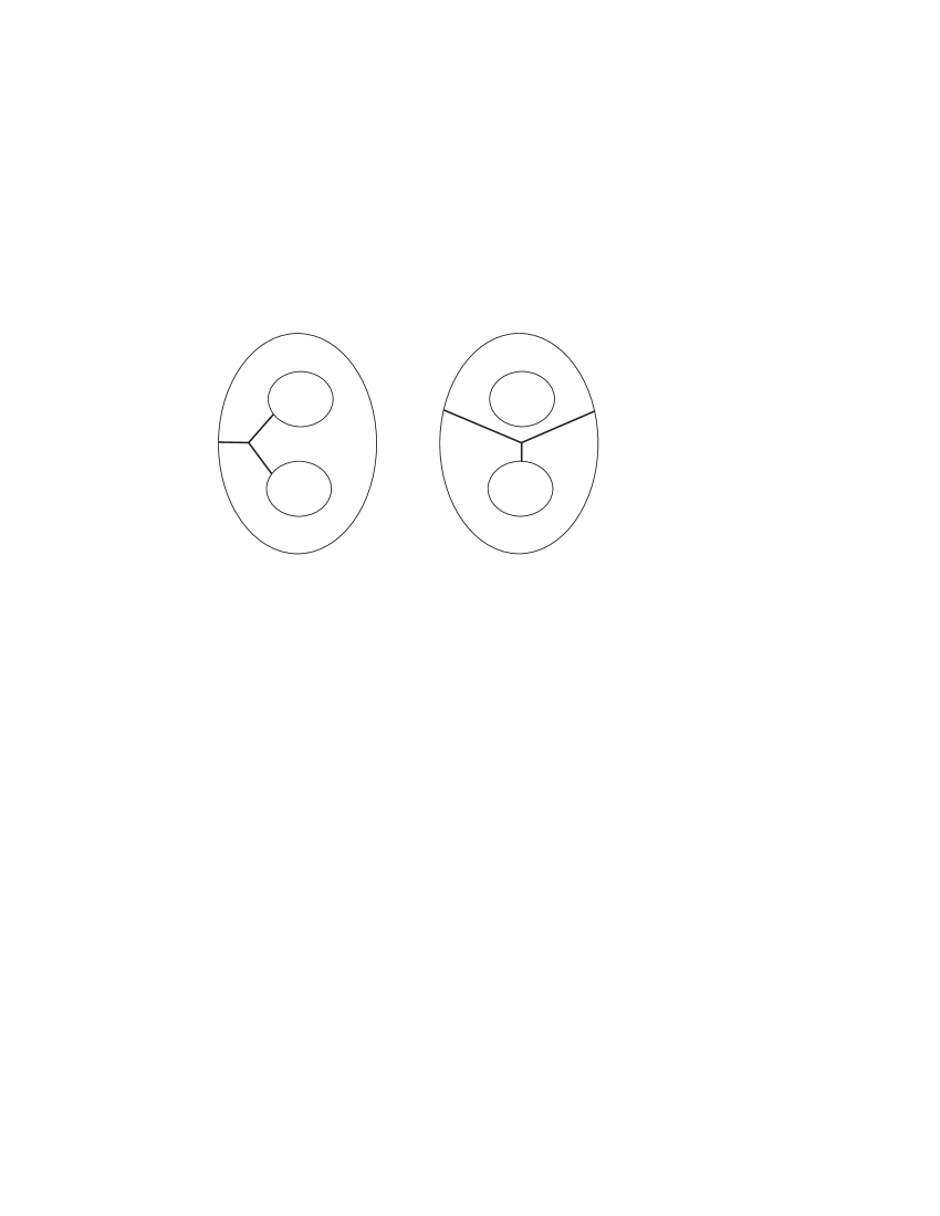
Elementary moves on pants decompositions. An elementary move on a maximal curve system $P$ is a replacement of a component $\alpha$ of $P$ by $\alpha^{\prime}$, disjoint from the rest of $P$, so that $\alpha$ and $\alpha^{\prime}$ are in one of the two configurations shown in Figure 1.

Figure 1. The two types of elementary moves.

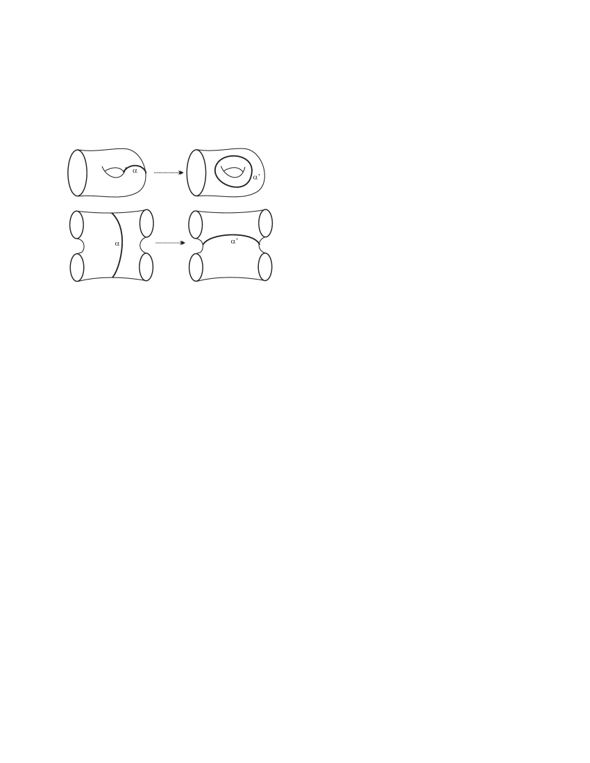
We indicate this by $P\to P^{\prime}$ where $P^{\prime}=P\setminus\{\alpha\}\cup\{\alpha^{\prime}\}$ is the new curve system. Note that there are infinitely many choices for $\alpha^{\prime}$, naturally indexed by ${\mathbb{Z}}$.

In Section 4 we will show how to relate these moves to controlled homotopies between pleated surfaces in $N_{\rho}$. In Section 5 we will describe the combinatorial aspects of connecting any two pants decompositions by an efficient sequence of elementary moves.

2.3. Unmeasured laminations and the boundary of ${\mathcal{C}}(S)$

In addition to being the space of ending laminations for $\rho\in{\mathcal{D}}_{\mathrm{np}}(S)$, $\operatorname{{\mathcal{E}}{\mathcal{L}}}(S)$ also has an interpretation as the Gromov boundary $\partial{\mathcal{C}}(S)$ of the $\delta$-hyperbolic space ${\mathcal{C}}(S)$ (see e.g. [17, 23, 22, 2, 7] for material on $\delta$-hyperbolicity).

In the following theorem note that ${\mathcal{C}}_{0}(S)$ can be considered as a subset of $\operatorname{{\mathcal{U}}{\mathcal{M}}{\mathcal{L}}}(S)$.

Theorem 2.1.

(Klarreich [33]) There is a homeomorphism

$$k:\partial{\mathcal{C}}(S)\to\operatorname{{\mathcal{E}}{\mathcal{L}}}(S),$$

which is natural in the sense that a sequence $\{\beta_{i}\in{\mathcal{C}}_{0}(S)\}$ converges to $\beta\in\partial{\mathcal{C}}(S)$ if and only if it converges to $k(\beta)$ in $\operatorname{{\mathcal{U}}{\mathcal{M}}{\mathcal{L}}}(S)$.

2.4. Pleated surfaces and uniform injectivity

A pleated surface is a map $f:S\to N$ together with a hyperbolic metric on $S$, written $\sigma_{f}$ and called the induced metric, and a $\sigma_{f}$-geodesic lamination $\lambda$ on $S$, so that the following holds: $f$ is length-preserving on paths, maps leaves of $\lambda$ to geodesics, and is totally geodesic on the complement of $\lambda$. Pleated surfaces were introduced by Thurston [52]. See Canary-Epstein-Green [16] for more details.

The set of all pleated surfaces (in fact all maps $S\to N_{\rho}$) admits a standard equivalence relation, in which $f\sim f\circ h$ if $h$ is a homeomorphism of $S$ isotopic to the identity. Let us refer to this as equivalence up to domain isotopy.

If $P$ is a curve or arc system, i.e. a simplex in ${\mathcal{A}}(S)$, let

$$\operatorname{\mathbf{pleat}}_{\rho}(P)$$

denote the set of pleated surfaces $f:S\to N_{\rho}$, in the homotopy class determined by $\rho$, which map representatives of $P$ to geodesics. Thurston observed that such maps always exist provided $P$ has no closed component which is parabolic in $\rho$. Let $\operatorname{\mathbf{pleat}}_{\rho}$ denote the set of all pleated surfaces in the homotopy class of $\rho$.

Note, if $P$ contains an arc terminating in punctures, the corresponding leaf in the lamination will be infinite and properly embedded in $S$, its ends exiting the cusps.

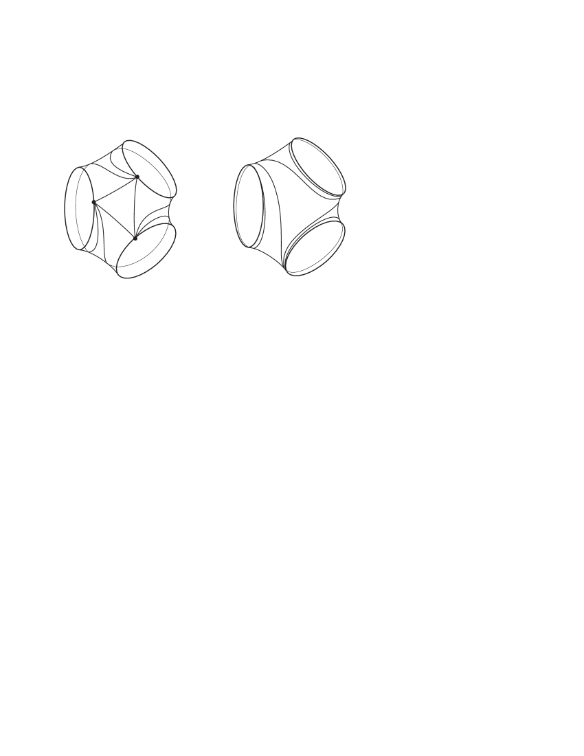
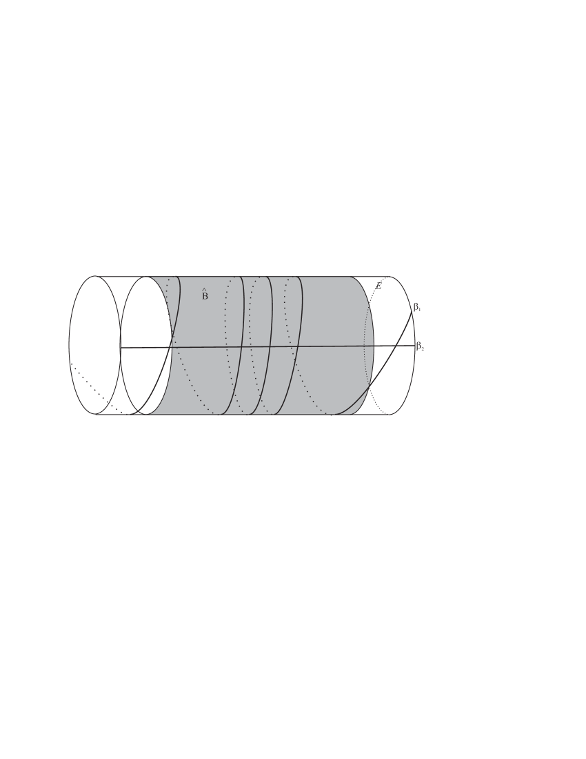
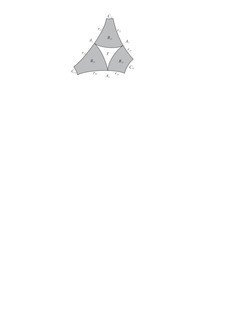
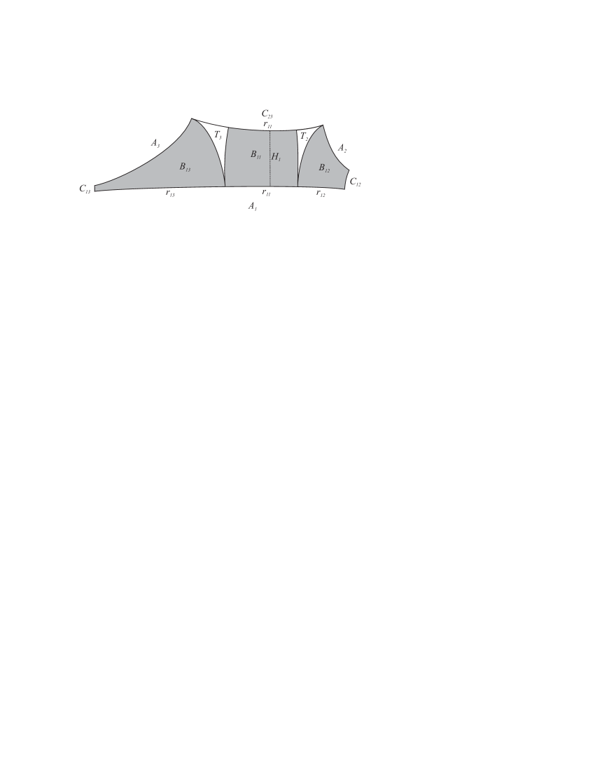
In particular, if $P$ is a maximal curve system, or “pants decomposition”, $\operatorname{\mathbf{pleat}}_{\rho}(P)$ consists of finitely many equivalence classes, all constructed as follows: Extend $P$ to a triangulation of $S$ with one vertex on each component of $P$ (and a vertex in each puncture, if any) and “spin” this triangulation around $P$, arriving at a lamination $\lambda$ whose closed leaves are $P$ and whose other leaves spiral onto $P$, as in Figure 2, or go out the cusps.

Figure 2. The lamination obtained by spinning a triangulation around a curve system. The picture shows one pair of pants in a decomposition.

Uniform Injectivity

Thurston’s Uniform Injectivity theorem for pleated surfaces [54] has two corollaries that we will use here. For further discussion and proofs see [42], [47] and also Brock [10].

Bridge arcs. If $\alpha$ is a lamination in $S$, a bridge arc for $\alpha$ is an arc in $S$ with endpoints on $\alpha$, which is not deformable rel endpoints into $\alpha$. A primitive bridge arc is a bridge arc whose interior is disjoint from $\alpha$. If $\sigma$ is a hyperbolic metric on $S$ and $\tau$ is a bridge arc for $\alpha$, let $[\tau]$ denote the homotopy class of $\tau$ with endpoints fixed, and for a metric $\sigma$ let $\ell_{\sigma}([\tau])$ denote the length of the minimal representative of $[\tau]$.

For a lamination $\mu$ and two maps $g,g^{\prime}\in\operatorname{\mathbf{pleat}}_{\rho}(\mu)$, we say that $g$ and $g^{\prime}$ are homotopic relative to $\mu$ if there is a homotopy between them fixing $\mu$ pointwise. Lemma 3.3 in [47] guarantees that we can always precompose $g^{\prime}$ by a homeomorphism isotopic to the identity to obtain a map that is homotopic to $g$ relative to $\mu$.

Let ${\mathbf{P}}{\mathbb{H}}^{3}$ denote the tangent line bundle over ${\mathbb{H}}^{3}$. For $g\in\operatorname{\mathbf{pleat}}_{\rho}$ mapping a lamination $\mu$ geodesically, and a bridge arc $\tau$ of $\mu$, define $d_{\mathbf{p}}(g(\tau))$ as follows: Lift $g(\tau)$ to an arc $\widetilde{g}(\tau)$ in ${\mathbb{H}}^{3}$ connecting two leaves of the lift of $g(\mu)$. The endpoints of $\widetilde{g}(\tau)$ and the leaves on which they lie determine two points in ${\mathbf{P}}{\mathbb{H}}^{3}$, and we let $d_{\mathbf{p}}(g(\tau))$ be their distance. In other words, $d_{\mathbf{p}}$ is small when the two leaves are both close together and nearly tangent.

The following strengthening of Thurston’s Uniform Injectivity theorem is essentially Lemma 3.4 in [47], which follows from Lemma 2.3 in [42].

Lemma 2.2.

(Short bridge arcs)  Fix the surface $S$. Given $\delta_{1}>0$ there exists $\delta_{0}\in(0,\delta_{1})$ such that the following holds.

Let $\rho\in{\mathcal{D}}(S)$ and let $g\in\operatorname{\mathbf{pleat}}_{\rho}$, mapping a lamination $\mu$ geodesically. Suppose that $\tau$ a bridge arc for $\mu$ which is either primitive, or contained in the $\epsilon_{1}$-thick part of $\sigma_{g}$. Then

$$d_{\mathbf{p}}(g(\tau))\leq\delta_{0}\implies\ell_{\sigma_{g}}([\tau])\leq\delta_{1}.$$

Moreover if $g^{\prime}$ is another map in $\operatorname{\mathbf{pleat}}_{\rho}(\mu)$, chosen so it is homotopic to $g$ relative to $\mu$, then

$$\ell_{\sigma_{g}}([\tau])\leq\delta_{0}\implies\ell_{\sigma_{g^{\prime}}}([\tau])\leq\delta_{1}.$$

The second statement follows from the first, since the short bridge arc in $\sigma_{g}$ connects two leaves that contain two segments that remain close to each other for roughly $|\log\delta_{0}|$, thus the same is true for their images by $g$ (hence by $g^{\prime}$). We get a bound on $d_{\mathbf{p}}(g^{\prime}(\tau))$ and up to revising the constants we have the desired statement.

Efficiency of pleated surfaces. Thurston also used Uniform Injectivity to establish an estimate relating lengths of curves in a pleated surface to their lengths in the 3-manifold. In order to state it we need the alternation number

$$a(\lambda,\gamma)$$

where $\lambda$ is a lamination with finitely many leaves and $\gamma$ is a simple closed curve (more generally a measured lamination. This quantity, a sort of refined intersection number, is defined carefully in Thurston [51] and Canary [15]. For our purposes we need only the following observations: a finite-leaved lamination consists of finitely many closed leaves, and finitely many infinite leaves whose ends spiral around the closed leaves. If $\gamma$ crosses only infinite leaves of $\lambda$, then $a(\lambda,\gamma)$ is bounded by the number of intersection points with $\lambda$.

The following statement is a slight generalization of the theorem proved in [51, Thm 3.3]. Thurston sketches the argument for this generalization, and it also follows from a relative version of the theorem proved in [47].

Theorem 2.3.

(Efficiency of pleated surfaces)  Given $S$ and any $\epsilon>0$, there is a constant $C>0$ for which the following holds.

Let $\rho\in{\mathcal{D}}(S)$ and suppose $g\in\operatorname{\mathbf{pleat}}_{\rho}$ maps geodesically a maximal finite-leaved lamination $\lambda$ Suppose $\gamma$ is a measured geodesic lamination in $(S,\sigma_{g})$ which does not intersect any closed curve of $\lambda$ whose length is less than $\epsilon$. Then

$$\ell_{\rho}(\gamma)\leq\ell_{\sigma_{g}}(\gamma)\leq\ell_{\rho}(\gamma)+Ca(\lambda,\gamma).$$ (2.1)

2.5. Margulis tubes

We shall denote by ${\mathbf{T}}_{\alpha}(\epsilon)$ the $\epsilon$-Margulis tube in $N_{\rho}$ for a closed curve $\alpha$ in hyperbolic manifold, that is the region where $\alpha$ can be represented with length at most $\epsilon$. We let $\epsilon_{0}$ be a Margulis constant for 2 and 3 dimensions, meaning that ${\mathbf{T}}_{\alpha}(\epsilon_{0})$ is always a solid torus neighborhood of a closed geodesic, or a horoball neighborhood of a cusp, and any two such tubes are disjoint. We also choose $\epsilon_{0}$ sufficiently small that, on a hyperbolic surface, any simple closed geodesic is disjoint from any $\epsilon_{0}$-Margulis tube but its own.

If $\rho\in{\mathcal{D}}(S)$ is fixed, we will usually use ${\mathbf{T}}_{\alpha}$ to denote ${\mathbf{T}}_{\rho(\alpha)}$, where $\alpha$ is a conjugacy class in $\pi_{1}(S)$.

The radius of an $\epsilon$-Margulis tube grows as the length of the core curve shrinks (see Brooks-Matelski [11] and Meyerhoff [41]). We shall need to use the following facts. First, if $\ell_{\rho}(\alpha)<\epsilon<\epsilon_{0}$ then the radius of ${\mathbf{T}}_{\alpha}(\epsilon_{0})$ is at least ${\textstyle{\frac{1}{2}}}\log(\epsilon_{0}/\epsilon)-c$ for a universal $c$. Second, the distance from ${\mathbf{T}}_{\alpha}(\epsilon/2)$ to $\partial{\mathbf{T}}_{\alpha}(\epsilon)$, if the former is non-empty, is uniformly bounded away from $0$ and $\infty$.

Margulis tubes in surface groups. Thurston observed that a constant $\epsilon_{1}$ exists, depending only on $S$, so that for any $\rho\in{\mathcal{D}}(S)$, if a pleated surface $g\in\operatorname{\mathbf{pleat}}_{\rho}$ meets ${\mathbf{T}}_{\alpha}(\epsilon_{1})$ it can only do so in its own $\epsilon_{0}$-Margulis tube. Thus $\alpha$ (if it is a primitive element) must be homotopic to the core of this tube in $S$, and in particular simple. Together with Bonahon’s tameness theorem [5], which implies that every point in $C(N_{\rho})$ is within a bounded distance of a pleated surface, we have that $\epsilon_{1}$ can be chosen so that $\ell_{\rho}(\alpha)<\epsilon_{1}$ implies that $\alpha$ is simple.

In the remainder of the paper, we fix $\epsilon_{1}$ so that it has these properties, and in addition $\epsilon_{1}<\epsilon_{0}/K_{0}$, where $K_{0}$ is the constant in Sullivan’s theorem (see §2.1) relating $\nu_{\pm}$ to $\nu^{\prime}_{\pm}$. This has the effect that a curve which is not externally short has length at least $\epsilon_{1}$ in $\nu^{\prime}_{\pm}$ as well as $\nu_{\pm}$.

2.6. The projection coefficients

Let us now see how to define the coefficients

$$d_{Y}(\nu_{+},\nu_{-})$$

which appear in the main theorem, where $\nu_{\pm}$ are end invariants for some $\rho\in{\mathcal{D}}_{\mathrm{np}}(S)$, and $Y$ is any essential subsurface of $S$.

Using $\pi_{Y}$ as above, we can already define this whenever $\nu_{\pm}$ are laminations. In the case of a geometrically finite end when $\nu_{+}$ or $\nu_{-}$ are hyperbolic metrics, we can extend this definition as follows:

A theorem of Bers (see [3, 4] and Buser [12]) says that a constant $L_{1}$ exists, depending only on the topological type of $S$, so that for any hyperbolic metric on $S$ there is a maximal curve system (a pants decomposition) with total length bounded by $L_{1}$. Moreover, $L_{1}$ can be chosen so that, if $\alpha$ is a geodesic of length at least $\epsilon_{1}$ (the constant defined in §2.5), a pants decomposition can be chosen with length bounded by $L_{1}$, and intersecting $\alpha$ essentially. Fix this constant for the remainder of the paper.

Now we define

$$\operatorname{\mathbf{short}}(\sigma)$$

to be the set of curve systems of $S$ with total $\sigma$-length at most $L_{1}$.

Thus e.g. if both $\nu_{+}$ and $\nu_{-}$ are hyperbolic structures, we may consider distances

$$d_{Y}(P_{+},P_{-})$$

for any $P_{\pm}\in\operatorname{\mathbf{short}}(\nu_{\pm})$ that both intersect $Y$ essentially, and notice that the numbers obtained cannot vary by more than a uniformly bounded constant (because two different curves in $\operatorname{\mathbf{short}}(\sigma)$ have a bounded intersection number, depending only on $L_{1}$). We let $d_{Y}(\nu_{+},\nu_{-})$ be, say, the minimum over all choices. The case when one of $\nu_{\pm}$ is a lamination and the other is a hyperbolic metric is handled similarly.

This defines $d_{Y}(\nu_{+},\nu_{-})$ for all $Y$, with the exception of an annulus whose core curve has length less than $\epsilon_{1}$ in one of $\nu_{+}$ or $\nu_{-}$, and a three-holed sphere all of whose boundary curves have this property. The case of three-holed spheres will not make any difference, since at any rate their curve complexes are finite. The case of annuli will require a bit of attention at the end of the proof of the main theorem.

3. Quasiconvexity of the bounded curve set

Let ${\mathcal{C}}(\rho,L)$ denote the subcomplex of ${\mathcal{C}}(S)$ spanned by the vertices with $\rho$-length at most $L$. In this section we will show that this set has certain quasiconvexity properties. Before stating them we will need to define a map

$$\Pi_{\rho}:{\mathcal{A}}(S)\to{\mathcal{P}}({\mathcal{C}}(\rho,L_{1}))$$

where ${\mathcal{P}}(X)$ denotes the set of subsets of $X$. Given $x\in{\mathcal{A}}(S)$ let $P_{x}$ be the curve/arc system associated to the smallest simplex containing $x$. We define

$$\Pi_{\rho}(x)=\bigcup_{f\in\operatorname{\mathbf{pleat}}_{\rho}(P_{x})}\operatorname{\mathbf{short}}(\sigma_{f}).$$

For convenience we will often write $\Pi_{\rho}(P)$ where $P$ is a curve/arc system.

In the following theorem, a set $A$ in a geodesic metric space is $b$-quasiconvex if every geodesic with endpoints in $A$ is contained in the $b$-neighborhood of $A$.

Theorem 3.1.

(Quasiconvexity)  For any $\rho\in{\mathcal{D}}(S)$ and $L\geq L_{1}$, ${\mathcal{C}}(\rho,L)$ is $B$-quasiconvex, where $B$ depends only on $L$ and the topology of $S$.

Moreover, if $\beta$ is a geodesic in ${\mathcal{C}}(S)$ with endpoints in ${\mathcal{C}}(\rho,L)$ then

$$d_{\mathcal{C}}(x,\Pi_{\rho}(x))\leq B$$

for each $x\in\beta$.

This will follow from the Coarse Projection lemma below, together with the hyperbolicity of ${\mathcal{C}}(S)$, via the argument in Lemma 3.3.

The coarse projection property

Lemma 3.2.

(Coarse Projection)  For any $\rho\in{\mathcal{D}}(S)$ the map $\Pi_{\rho}$ satisfies the following:

1. (Coarse Lipschitz) If $d_{\mathcal{A}}(x,y)\leq 1$ then

   $$\operatorname{diam}_{\mathcal{C}}(\Pi_{\rho}(x)\cup\Pi_{\rho}(y))\leq b.$$

2. (Coarse idempotence) If $x\in{\mathcal{C}}(\rho,L_{1})$ then

   $$d_{\mathcal{C}}(x,\Pi_{\rho}(x))=0$$

where $b$ depends only on $S$.

Note that here distance between sets (as in property (2)) is the minimal distance, whereas $\operatorname{diam}_{\mathcal{C}}$ controls maximal distances.

Proof.

Property (2) (Coarse idempotence) is immediate from the definition, since for any $f\in\operatorname{\mathbf{pleat}}_{\rho}(x)$, $x$ is realized in $\sigma_{f}$ with its minimal length, and so is included in $\operatorname{\mathbf{short}}(\sigma_{f})$.

Note next that there exists $B=B(L_{1})$ such that, for any hyperbolic structure $\sigma$,

$$\operatorname{diam}_{\mathcal{C}}(\operatorname{\mathbf{short}}(\sigma))<B$$ (3.1)

since there is a uniform bound on the intersection number of any two curves of length at most $L_{1}$ in the same metric on $S$.

Now to prove part (1), it clearly suffices to consider $x,y\in{\mathcal{A}}_{0}(S)$. The condition $d(x,y)=1$ means $x$ and $y$ are disjoint, so $x\cup y$ is a curve/arc system, and since

$$\Pi_{\rho}(x\cup y)\subset\Pi_{\rho}(x)\cap\Pi_{\rho}(y),$$

the intersection is non-empty. Thus it will suffice to obtain a bound of the form

$$\operatorname{diam}_{\mathcal{C}}(\Pi_{\rho}(\gamma))\leq B$$ (3.2)

for any curve/arc system $\gamma$. To do this we must compare the short curves in any two different surfaces pleated along $\gamma$. Let $f,g\in\operatorname{\mathbf{pleat}}_{\rho}(\gamma)$, and assume (see discussion in §2.4) that they are homotopic relative to $\gamma$.

Suppose first that $\gamma$ meets the (non-cuspidal) $\epsilon_{1}$-thin part of $\sigma_{f}$. Then its $f$-image meets the $\epsilon_{1}$-thin part of $N_{\rho}$, and hence so does its $g$-image (since they agree). Let $\alpha$ be the core curve of this component of the thin part. The length of $\alpha$ in $\sigma_{g}$ must also be at most $\epsilon_{0}$ (by the choice of $\epsilon_{1}$ in §2.5), and in particular

$$\alpha\in\operatorname{\mathbf{short}}(\sigma_{f})\cap\operatorname{\mathbf{short}}(\sigma_{g}).$$

Together with (3.1), this implies a bound on

$$\operatorname{diam}_{\mathcal{C}}(\operatorname{\mathbf{short}}(\sigma_{f})\cup\operatorname{\mathbf{short}}(\sigma_{g})).$$

The bound (3.2) follows.

Now suppose that $\gamma$ stays in the $\epsilon_{1}$-thick part of $\sigma_{f}$, except possibly for cusps ($\gamma$ may contain an infinite leaf terminating in a cusp).

By the second part of Lemma 2.2, there exists an $\epsilon>0$ so that, if $\tau$ is a bridge arc for $\gamma$ in the $\epsilon_{1}$-thick part of $\sigma_{f}$ and whose $\sigma_{f}$-length is at most $\epsilon$, then $\tau$ is homotopic rel endpoints to an arc of $\sigma_{g}$-length $\epsilon_{0}$.

Given this $\epsilon$, we may construct a homotopically non-trivial curve $\gamma_{\epsilon}$ in the $\epsilon_{1}$-thick part of $\sigma_{f}$, whose $\sigma_{f}$-length is at most a constant $L_{2}$, and which is composed of at most two arcs of $\gamma$ and at most two primitive bridge arcs of length $\epsilon$ or less. (The proof is a standard argument, which we sketch in Lemma 8.5).

The bridge arcs can be homotoped to have $\sigma_{g}$ length at most $\epsilon_{0}$, and hence $\gamma_{\epsilon}$ can be realized in $\sigma_{g}$ with length at most $L_{2}+2\epsilon_{0}$. In each surface this bounds its ${\mathcal{C}}$-distance from the curves of length $L_{1}$, and together with (3.1) we again obtain a bound on

$$\operatorname{diam}_{\mathcal{C}}(\operatorname{\mathbf{short}}(\sigma_{f})\cup\operatorname{\mathbf{short}}(\sigma_{g})),$$

and the desired bound (3.2) follows. ∎

Proof of Quasiconvexity

The Quasiconvexity theorem follows from the Coarse Projection lemma via the following standard argument, which has its roots in the proof of Mostow’s rigidity theorem (the difference between this and the standard argument is the need to consider two projections, to a geodesic and to the candidate quasiconvex set, whereas the standard argument involves only projection to a geodesic).

Lemma 3.3.

Let $X$ be a $\delta$-hyperbolic geodesic metric space and $Y\subset X$ a subset admitting a map $\Pi:X\to Y$ which is coarse-Lipschitz and coarse-idempotent. That is, there exists $C>0$ such that

• If $d(x,x^{\prime})\leq 1$ then $d(\Pi(x),\Pi(x^{\prime}))\leq C$, and

• If $y\in Y$ then $d(y,\Pi(y))\leq C.$

Then $Y$ is quasi-convex, and furthermore if $g$ is a geodesic in $X$ whose endpoints are within distance $a$ of $Y$ then

$$d(x,\Pi(x))\leq b$$

for some $b=b(a,\delta,C)$, and every $x\in g$.

Proof.

The condition of $\delta$-hyperbolicity for $X$ implies that for any geodesic $g$ (finite or infinite) the closest-points projection $\pi_{g}:X\to g$ is coarsely contracting in this sense: If $x\in X$ and $r=d(x,g)$ then the ball $B_{r}(x)$ has $\pi_{g}$-image whose diameter is bounded by a constant $b_{0}$ depending only on $\delta$. (This is an easy exercise in the definitions – see e.g. [23, 22, 2, 7]. Indeed this condition for all geodesics $g$ implies $\delta$-hyperbolicity [36]).

In the rest of the proof, let a “dotted path” be a sequence $p=\{x_{i}\in X\}$ with $d(x_{i},x_{i+1})\leq C$, and let its “length” be $l(p)=\sum_{i}d(x_{i},x_{i+1})$. Let $r>C$. If $p$ is a dotted path in $X$ outside an $r$-neighborhood of $g$ then the contraction property of the previous paragraph implies

$$l(p)\geq(r-C)\left(\frac{1}{b_{0}}\operatorname{diam}(\pi_{g}(p))-1\right).$$ (3.3)

Now suppose that $g$ has endpoints within $a$ of $Y$ and assume also that $r>a$. Let $J$ be a segment of $g$ whose endpoints $\xi,\eta$ are within $r$ of $x,y\in Y$, respectively, but whose interior is outside the $r$-neighborhood of $Y$. On the concatenation of geodesics from $x$ to $\xi$, across $J$ to $\eta$ and back to $y$, select a sequence of points spaced at most 1 apart and apply $\Pi$, obtaining (via the coarse-Lipschitz property) a dotted path $p$ in $Y$ satisfying

$$l(p)\leq C(2r+l(J)+1)$$

by the coarse-Lipschitz property. Since $x$ and $y$ are distance $C$ from the respective endpoints $\Pi(x)$ and $\Pi(y)$ of $p$ (by coarse idempotence) and $r>C$, the contraction property of $\pi_{J}$ implies that $\pi_{J}(\Pi(x))$ and $\pi_{J}(\Pi(y))$ are within $b_{0}$ of $\pi_{J}(x)=\xi$ and $\pi_{J}(y)=\eta$ respectively. It follows that $\operatorname{diam}(\pi_{J}(p))\geq l(J)-2b_{0}$. Thus, together with (3.3) we obtain

$$(r-C)\left(\frac{1}{b_{0}}(l(J)-2b_{0})-1\right)\leq l(p)\leq C(2r+l(J)+1),$$

and hence

$$\left(\frac{r-C}{b_{0}}-C\right)l(J)\leq 3(r-C)+C(2r+1).$$

Now if we choose $r$ so that $\frac{r-C}{b_{0}}-C\geq 1$, we obtain an upper bound

$$l(J)\leq 3(r-C)+C(2r+1).$$

This bounds by $b_{1}=r+{\textstyle{\frac{1}{2}}}(3(r-C)+C(2r+1))$ the maximum distance from a point in $J$ to $Y$. Since this applies to every excursion of $g$ from the $r$-neighborhood of $Y$, we conclude that $Y$ is $b_{1}$-quasi-convex.

Now let $x\in g$ be any point. We have the bound $d(x,Y)\leq b_{1}$. Let $y\in Y$ be a nearest point to $x$. We have $d(y,\Pi(y))\leq C$ by coarse idempotence. Now applying coarse Lipschitz to the path from $y$ to $x$, whose length is at most $b_{1}$, we find that $d(\Pi(x),\Pi(y))$ is at most $C(b_{1}+1)$. Finally by the triangle inequality we obtain a bound on $d(x,\Pi(x))$. ∎

To apply this lemma to our setting, we recall first that in [36] we proved that ${\mathcal{C}}(S)$, and hence ${\mathcal{A}}(S)$, is $\delta$-hyperbolic. Our map $\Pi_{\rho}$ has images that are subsets of ${\mathcal{C}}(S)$ rather than single points, but this can easily be remedied by choosing any method at all to select a single point from each set $\Pi_{\rho}(x)$. Lemma 3.2 implies that the resulting map has the properties required in Lemma 3.3. ∎

4. Elementary moves on pleated surfaces

In this section we will show how to realize an elementary move between two pants decompositions $P_{0}$ and $P_{1}$ of $S$ as a controlled homotopy between pleated surfaces in $\operatorname{\mathbf{pleat}}_{\rho}(P_{0})$ and $\operatorname{\mathbf{pleat}}_{\rho}(P_{1})$. Lemma 4.1 will show that two surfaces that are “good” with respect to a single pants decomposition admit a controlled homotopy. Lemma 4.2 shows that a pleated surface exists which is “good” for both $P_{0}$ and $P_{1}$ simultaneously. Thus we can concatenate a controlled homotopy from a surface in $\operatorname{\mathbf{pleat}}_{\rho}(P_{0})$ to the halfway surface, with one from the halfway surface to a surface in $\operatorname{\mathbf{pleat}}_{\rho}(P_{1})$.

We begin with some definitions. Let $\operatorname{\mathbf{collar}}(\gamma,\sigma)$ denote the standard collar for $\gamma$ in the surface $S$ with metric $\sigma$, as defined in Section 8. Similarly define $\operatorname{\mathbf{collar}}(P,\sigma)$ for a curve system $P$.

Good maps: If $P$ is a curve system in $S$, we let

$$\operatorname{\mathbf{good}}_{\rho}(P,C)$$

denote the set of pleated maps $g:S\to N_{\rho}$ in the homotopy class determined by $\rho$, such that

$$\ell_{\sigma_{g}}(\gamma)\leq\ell_{\rho}(\gamma)+C$$

for all components $\gamma$ of $P$. Note that

$$\operatorname{\mathbf{pleat}}_{\rho}(P)\subset\operatorname{\mathbf{good}}_{\rho}(P,C)$$

for any $C\geq 0$.

Good homotopies: Let $f,g\in\operatorname{\mathbf{pleat}}_{\rho}$ and let $P$ be a curve system. We say that $f$ and $g$ admit a $K$-good homotopy with respect to $P$ if there exists a homotopy $H:S\times[0,1]\to N_{\rho}$ such that the following holds:

1. $H_{0}\sim f$ and $H_{1}\sim g$ up to domain isotopy (§2.4).

2. Denoting by $\sigma_{i}$ the induced metric by $H_{i}$ for $i=0,1$,

   $$\operatorname{\mathbf{collar}}(P,\sigma_{0})=\operatorname{\mathbf{collar}}(P,\sigma_{1}).$$

   We henceforth omit the metric when referring to these collars.

3. The metrics $\sigma_{0}$ and $\sigma_{1}$ are locally $K$-bilipschitz outside $\operatorname{\mathbf{collar}}(P)$.

4. Let $P_{0}$ denote the subset of $P$ consisting of curves $\gamma$ with $\ell_{\rho}(\gamma)<\epsilon_{0}$. The tracks $H(p\times[0,1])$ are bounded in length by $K$ when $p\notin\operatorname{\mathbf{collar}}(P_{0})$.

5. For each $\alpha\in P_{0}$, the image $H(\operatorname{\mathbf{collar}}(\alpha)\times[0,1])$ is contained in a $K$-neighborhood of the Margulis tube ${\mathbf{T}}_{\alpha}(\epsilon_{0})$.

The homotopy bound lemma

Lemma 4.1.

(Homotopy bound)  Given $C$ there exists $K$ so that for any $\rho\in{\mathcal{D}}_{\mathrm{np}}(S)$ and maximal curve system $P$, if

$$f,g\in\operatorname{\mathbf{good}}_{\rho}(P,C)$$

then $f$ and $g$ admit a $K$-good homotopy with respect to $P$.

Proof.

Let us first give the proof in the case that $S$ is a closed surface. At the end we will remark on the changes necessary to allow cusps.

Since the $\sigma_{f}$ and $\sigma_{g}$ lengths of the components of $P$ differ by at most an additive constant $C$, Lemma 8.2 (applied to each component of $S\setminus P$) gives us a homeomorphism $\varphi:S\to S$ isotopic to the identity, which takes $\operatorname{\mathbf{collar}}(P,\sigma_{f})$ to $\operatorname{\mathbf{collar}}(P,\sigma_{g})$ and is locally $K$-bilipschitz in its complement, with $K$ depending only on $C$. Moreover arclengths on $\partial\operatorname{\mathbf{collar}}(P,\sigma_{f})$ are additively distorted in a bounded way: if $\alpha\subset\partial\operatorname{\mathbf{collar}}(P,\sigma_{f})$ is any arc then $|l_{\sigma_{f}}(\alpha)-l_{\sigma_{g}}(\varphi(\alpha))|\leq K$. After replacing $g$ with $g\circ h$, we may assume $\operatorname{\mathbf{collar}}(P,\sigma_{f})=\operatorname{\mathbf{collar}}(P,\sigma_{g})$ (and henceforth denote it just $\operatorname{\mathbf{collar}}(P)$), and that $\sigma_{f}$ and $\sigma_{g}$ are locally $K$-bilipschitz off $\operatorname{\mathbf{collar}}(P)$, and have bounded additive length distortion on $\partial\operatorname{\mathbf{collar}}(P)$.

Now let $H:S\times[0,1]\to N_{\rho}$ be the homotopy between $f$ and $g$ whose tracks $H|_{\{x\}\times[0,1]}$ are geodesics parameterized at constant speed. ($H$ exists and is unique as a consequence of negative curvature and the fact that $\pi_{1}(S)$ is non-elementary, see e.g. [42]).

We will bound the tracks of $H$ on succesively larger parts of the surface.

Let $Y$ denote a component of $S\setminus P$, and let $Y_{0}=Y\setminus int(\operatorname{\mathbf{collar}}(\partial Y))$. We first remark that, in either $\sigma_{f}$ or $\sigma_{g}$, the length of any boundary component $\gamma$ of $Y_{0}$ is at most $2$ more than its corresponding geodesic in $S$, by (8.1), and this in turn is bounded by the assumption that $f,g\in\operatorname{\mathbf{good}}_{\rho}(P,C)$. Thus we have

$$l_{\sigma}(\gamma)\leq\ell_{\rho}(\gamma)+C+2$$ (4.1)

for $\sigma=\sigma_{f}$ or $\sigma_{g}$.

Bounds on the tripods. Let $\Delta$ be an essential tripod in $Y_{0}$ with legs of $\sigma_{f}$-length bounded by $\delta$, as given by Lemma 8.1 in the Appendix. Let $X$ be a component of the preimage of $\Delta$ in the universal cover $\widetilde{S}$. Lift $H$ to $\widetilde{H}:\widetilde{S}\times[0,1]\to{\mathbb{H}}^{3}$.

We claim there is a uniform bound on the lengths of the tracks $\widetilde{H}(\{x\}\times[0,1])$ for $x\in X$.

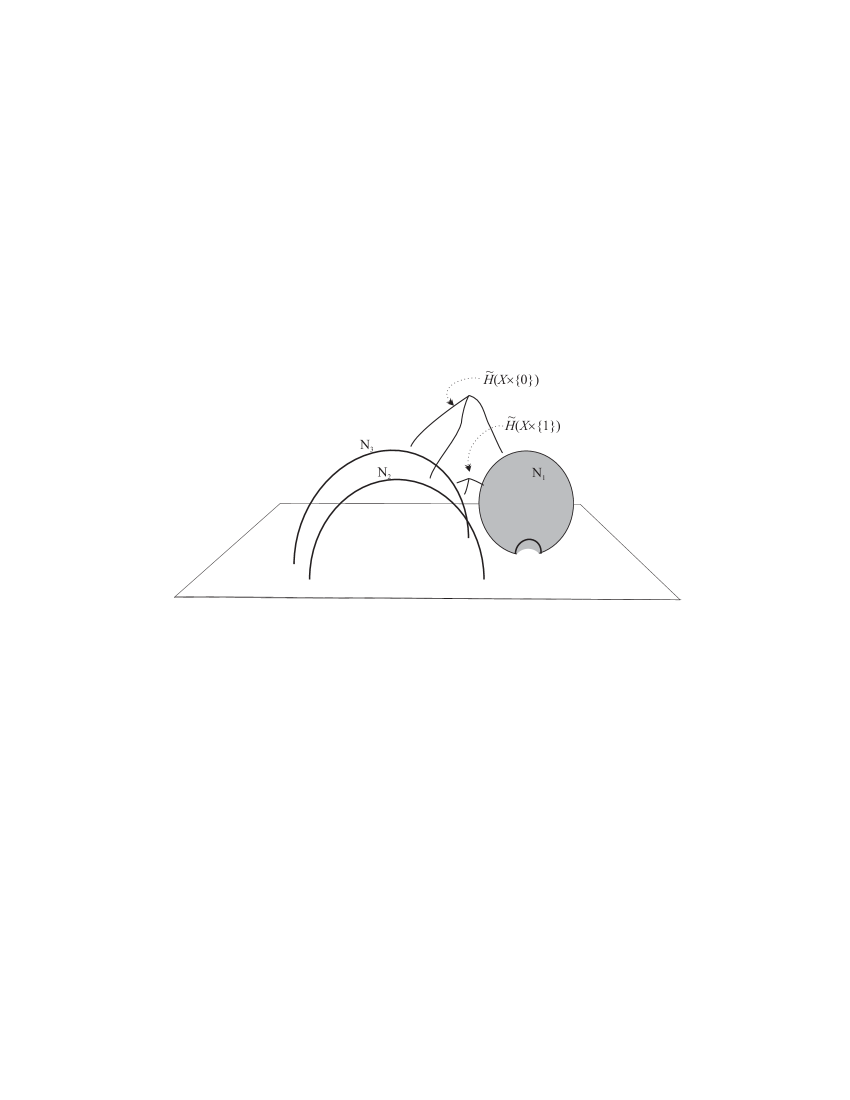
The image $\widetilde{H}(X\times\{0\})$ connects three lifts of boundary curves of $Y_{0}$, each invariant by a primitive deck translation $\gamma_{i}$ in $\rho(\pi_{1}(S))$ ($i=1,2,3$). Let $L_{i}$ be the axis of $\gamma_{i}$ (see Figure 3). If $\gamma_{i}$ has translation length less than $\epsilon_{1}/2$, define $N_{i}$ to be the lift of the corresponding $\epsilon_{0}$-Margulis tube in $N_{\rho}$. Otherwise define $N_{i}=L_{i}$.

Each image (under $f$ or $g$) of a boundary curve of $Y_{0}$ admits a homotopy to its geodesic representative in $N$, and because of the length bound (4.1), Lemma 8.4 tells us that this homotopy can, in uniformly bounded distance, be made to reach either the geodesic or its $\epsilon_{0}$-Margulis tube if it is short. Lifting to the universal cover, we conclude that the endpoints of $\widetilde{H}(X\times\{j\})$ ($j=0,1$) are within bounded distance of the corresponding $N_{i}$.

Since we have a uniform diameter bound $d_{0}=2K\delta$ on $\widetilde{H}(X\times\{0\})$ and $\widetilde{H}(X\times\{1\})$, we find that

$$\widetilde{H}(X\times\{j\})\subset{\mathcal{N}}_{d_{1}}(N_{1})\cap{\mathcal{N}}_{d_{1}}(N_{2})\cap{\mathcal{N}}_{d_{1}}(N_{3})$$ (4.2)

for $j=0,1$, with a uniform $d_{1}$. Here ${\mathcal{N}}_{r}$ denotes an $r$-neighborhood in ${\mathbb{H}}^{3}$.

Figure 3. The images of $X\times\{0\}$ and $X\times\{1\}$ are within uniform distance of the three invariant sets $N_{1},N_{2},N_{3}$.

The idea now is that, by virtue of discreteness, the triple intersection of the ${\mathcal{N}}_{d_{1}}(N_{i})$ cannot have very large diameter. Roughly, if the $N_{i}$ are Margulis tubes their strict convexity implies this, and if they are axes $L_{i}$ an application of Lemma 2.2 can be used to forbid the existence of long parallel sections. Once we prove this we will obtain a diameter bound on $\widetilde{H}(X\times[0,1])$, which will give the desired homotopy bound.

If one of the $N_{i}$ corresponds to a $\gamma_{i}$ of translation length less than $\epsilon_{1}/2$, let $N_{i}(\epsilon_{1})\subset N_{i}$ denote a lift of the corresponding $\epsilon_{1}$-Margulis tube. Note that $\operatorname{dist}(N_{i}(\epsilon_{1}),\partial N_{i})$ is uniformly bounded away from $0$ and $\infty$. If two of the $N_{i}$, say $N_{1}$ and $N_{2}$, are in this case, then they are disjoint, and hence their convex subsets $N_{i}(\epsilon_{1})$ are a definite distance apart. Applying Lemma 8.6 of the Appendix to $N_{1}(\epsilon_{1})$ and $N_{2}(\epsilon_{1})$, we can deduce that the intersection ${\mathcal{N}}_{d_{1}}(N_{1})\cap{\mathcal{N}}_{d_{1}}(N_{2})$ has diameter bounded by some $d_{2}$.

For the remainder of the argument, pick a pleated surface $h\in\operatorname{\mathbf{pleat}}_{\rho}(P)$.

Suppose that just $N_{1}$ corresponds to a curve of length less than $\epsilon_{1}/2$. We claim that $L_{2}$ is disjoint from $N_{1}(\epsilon_{1})$. Let $\gamma_{2}^{h}$ denote the $\sigma_{h}$-geodesic boundary component of $Y$ corresponding to to $\gamma_{2}$. If $L_{2}$ meets $N_{1}(\epsilon_{1})$ then $\gamma_{2}^{h}$ has $h$-image that meets an $\epsilon_{1}$-Margulis tube, and hence (by our choice of $\epsilon_{1}$) $\gamma_{2}^{h}$ meets the $\epsilon_{0}$-collar of another boundary component of $Y$ (in $S$ with the metric $\sigma_{h}$). By our choice of $\epsilon_{0}$, a simple geodesic cannot meet an $\epsilon_{0}$-Margulis tube in a surface unless it is the core of that tube, so this is a contradiction. Now $N_{1}(\epsilon_{1})$ contains the convex subset $N_{1}(\epsilon_{1}/2)$ which is definite distance from its boundary, and hence we can apply Lemma 8.6 to $N_{1}(\epsilon_{1}/2)$ and $L_{2}$, deducing a bound on $\operatorname{diam}({\mathcal{N}}_{d_{1}}(N_{1})\cap{\mathcal{N}}_{d_{1}}(N_{2}))$.

Finally suppose all three $\gamma_{i}$ have length at least $\epsilon_{1}/2$. Then in fact the three axes $\{L_{i}\}$ themselves come within bounded distance $2d_{3}$. If the intersection of all three ${\mathcal{N}}_{d_{3}}(L_{i})$ has diameter $D$ then $L_{1},L_{2}$ and $L_{3}$ contain segments of length at least $D-2d_{3}$ that remain distance $d_{3}$ apart. There are therefore two a-priori constants $d_{4},b>0$ so that there exists a point $p\in{\mathbb{H}}^{3}$ which is at most $\epsilon(D)=d_{4}e^{-bD}$ from all three $L_{i}$, and so that the tangent directions to $L_{i}$ at the points $x_{i}$ closest to $p$ are at most $2\epsilon(D)$ apart in ${\mathbf{P}}{\mathbb{H}}^{3}$.

Extend the tripod $\Delta$ to a tripod $\Delta^{\prime}$ with endpoints in $\partial Y$, and let $X^{\prime}$ be the component of its lift to $\widetilde{S}$ that contains $X$. The endpoints of $X^{\prime}$ are mapped by $\widetilde{h}$ to points $y_{i}\in L_{i}$ ($i=1,2,3$). The arcs $[y_{i},x_{i}]$ on $L_{i}$ pull back to arcs on $\partial Y$ which, if we append them to $\Delta^{\prime}$ and perturb slightly to an embedding in $Y$, give us a new tripod $\Delta^{\prime\prime}$ whose endpoints (after lifting and applying $\widetilde{h}$) map to $x_{i}$.

Let $\delta^{\prime}$ be the constant given in Lemma 8.1, and let $\delta_{0}$ be the constant given by Lemma 2.2 after setting $\delta_{1}=\delta^{\prime}$. Note that each pair of legs of $\Delta^{\prime\prime}$ is a primitive bridge arc for $\partial Y$, whose $h$-image is homotopic rel endpoints to an arc of length at most $2\epsilon(D)$. If $D$ is sufficiently large that $2\epsilon(D)<\delta_{0}$, then Lemma 2.2 tells us that each pair of legs of $\Delta^{\prime\prime}$ is homotopic to an arc of length at most $\delta_{1}$ in $\sigma_{h}$. This gives us a triangle in $Y$ with the same vertices as $\Delta^{\prime\prime}$ whose sidelengths are at most $\delta_{1}$. Joining its barycenter to its vertices we obtain a new tripod $\Delta^{\prime\prime\prime}$ all of whose legs are bounded by $\delta_{1}=\delta^{\prime}$. This contradicts Lemma 8.1. We conclude that the triple intersection of (4.2) has diameter at most $D$.

This diameter bound and (4.2) now imply a uniform bound on the track lengths of $\widetilde{H}$ restricted to $X$, and hence $H$ restricted to $\Delta$.

Bounds outside the collars. To bound the tracks of $H$ on the rest of $S\setminus\operatorname{\mathbf{collar}}(P)$, we first bound them on $\partial\operatorname{\mathbf{collar}}(P)$.

Let $\gamma$ be a component of $\partial\operatorname{\mathbf{collar}}(P)$. Let $Y$ be the component of $S\setminus P$ containing $\gamma$, so that $\gamma$ is in the boundary of $Y_{0}\equiv Y\setminus int(\operatorname{\mathbf{collar}}(\partial Y))$. Lemma 8.1 gives us a bounded essential tripod $\Delta$ in $Y_{0}$ with endpoint $x\in\gamma$. By the forgoing discussion we already have a bound, say $t_{0}$, on the track length $H(\{x\}\times[0,1])$.

If $\ell_{\rho}(\gamma)\leq 1$, we have the bound (4.1) on the $l_{\sigma_{f}}(\gamma)$ and $l_{\sigma_{g}}(\gamma)$. Via the triangle inequality we immediately get a bound on $H(\{y\}\times[0,1])$ for any $y\in\gamma$.

Suppose that $\ell_{\rho}(\gamma)>1$. Let $G=H|\gamma\times[0,1]$, and let $\widetilde{G}:\widetilde{\gamma}\times[0,1]\to{\mathbb{H}}^{3}$ be a lift to the universal covers. Lift $x$ to $\{x_{i}|i\in{\mathbb{Z}}\}$ in $\widetilde{\gamma}$. Let $\Gamma$ be the geodesic lift of $\gamma^{*}$ to ${\mathbb{H}}^{3}$ which is invariant by the holonomy of $\widetilde{G}$.

Because of the bound (4.1) on $l_{\sigma}(\gamma)$ (for $\sigma=\sigma_{f}$ or $\sigma_{g}$), we may apply Lemma 8.4 to either $\widetilde{G}_{0}=\widetilde{G}(\cdot,0)$ or $\widetilde{G}_{1}=\widetilde{G}(\cdot,1)$. For any $y\in\widetilde{\gamma}$ let $\eta_{i}=\pi(\widetilde{G}_{i}(y))$, where $\pi:{\mathbb{H}}^{3}\to\Gamma$ is the orthogonal projection. Then the lemma gives us, first, a bound

$$d(\widetilde{G}_{i}(y),\eta_{i})\leq a_{1}$$

and $i=0,1$.

Let $\xi_{ij}=\pi(\widetilde{G}_{i}(x_{j}))$. The main part of Lemma 8.4 tells us that for any $y\in[x_{0},x_{1}]$, its projection $\eta_{0}$ lies a bounded distance $a_{2}$ from the point in $[\xi_{00},\xi_{01}]$ that is at distance $|[x_{0},y]|_{f}$ from $\xi_{00}$. Here $|\cdot|_{f}$ and $|\cdot|_{g}$ denote the lifts of $\sigma_{f}$ and $\sigma_{g}$ arclength to $\widetilde{\gamma}$. Similarly we have a bound for $\eta_{1}$, $[\xi_{10},\xi_{11}]$ and $|[x_{0},y]|_{g}$.

The length bound on $G(x\times[0,1])$ tells us that $d(\xi_{0j},\xi_{1j})\leq 2a_{1}+t_{0}$. Since $|[x_{0},y]|_{f}$ and $|[x_{0},y]|_{g}$ differ by at most $K$ (via Lemma 8.2, as discussed in the beginning of the proof), we obtain a uniform upper bound on $d(\eta_{0},\eta_{1})$ and hence on the track length $\widetilde{G}(\{y\}\times[0,1])$.

This proves our uniform bound on the track lengths for $\partial\operatorname{\mathbf{collar}}(P)$.

Now for any point $z$ in $S\setminus\operatorname{\mathbf{collar}}(P)$ there is an arc $\beta$ connecting $z$ to some point $z^{\prime}$ in $\partial\operatorname{\mathbf{collar}}(P)$ whose length in either $\sigma_{f}$ or $\sigma_{g}$ is uniformly bounded. The length of $H(z^{\prime}\times[0,1])$ is bounded by the above, so we may bound $H(z\times[0,1])$ using the triangle inequality.

Bounds in the collars. It remains to control $H$ on $\operatorname{\mathbf{collar}}(P)\times[0,1]$. For each component $\gamma$ of $P$, $\operatorname{\mathbf{collar}}(\gamma)\times[0,1]$ is a solid torus, and we will control $H$ by considering a meridian curve

$$m=\partial(a\times[0,1])$$

where $a$ is an arc connecting the boundary components of $\operatorname{\mathbf{collar}}(\gamma)$.

Suppose first that $\ell_{\rho}(\gamma)\geq\epsilon_{0}$. Then the radius of $\operatorname{\mathbf{collar}}(\gamma)$ is bounded above by $s\equiv w(\epsilon_{0})$ in either $\sigma_{f}$ or $\sigma_{g}$. Let $a$ denote a minimal $\sigma_{f}$-length arc crossing $\operatorname{\mathbf{collar}}(\gamma)$, and let us find a bound on $L\equiv l_{\sigma_{g}}(a)$. (Note that up to the usual equivalence of maps we may assume $a$ is geodesic in both metrics).

Let $\gamma_{g}$ be the $\sigma_{g}$-geodesic representative of $\gamma$. We first replace $a$ by a homotopic path (with fixed endpoints) $q_{0}*a^{\prime}*q_{1}$ where $a^{\prime}$ is the $\sigma_{g}$-orthogonal projection of $a$ to $\gamma_{g}$, and $q_{i}$ are orthogonal segments to $\gamma_{g}$ of length at most $s$. Thus $l(a^{\prime})\geq L-2s$. Now apply Lemma 8.4 to deform $g(a^{\prime})$, fixing endpoints, to a path $p_{0}*a^{\prime\prime}*p_{1}$ in $N$ with $p_{i}$ of length bounded by $a_{1}$, $a^{\prime\prime}$ traveling along the geodesic representative of $\gamma$,

$$l_{N}(a^{\prime\prime})\geq c_{1}l(a^{\prime})-c_{2}$$

where $c_{1}$ and $c_{2}$ depend on the constants in the lemma. It follows that the geodesic representative of the path $g(a)$ in $N$ has length at least $c_{3}L-c_{4}$ for suitable constants $c_{3},c_{4}$.

Now consider a lift $\widetilde{H}(m)$ of the meridian to ${\mathbb{H}}^{3}$. The endpoints of $\widetilde{H}(a\times\{1\})$ are at least $c_{3}L-c_{4}$ apart, and on the other hand the other three legs of $m$ give us an upper bound of $2s+2t_{1}$, where $t_{1}$ is the track bound we have already obtained on $H$ outside the collars. This gives us an upper bound on $L$, and hence on the length of $H(m)$.

A bound on the tracks of $H$ follows immediately for any point of $a$, and since we can foliate $\operatorname{\mathbf{collar}}(\gamma)$ by arcs such as $a$, we obtain a bound in the entire collar.

Finally suppose that $\ell_{\rho}(\gamma)<\epsilon_{0}$, that is $\gamma\in P_{0}$. Since $\ell_{\sigma_{f}}(\gamma)$ and $\ell_{\sigma_{g}}(\gamma)$ are bounded by $\epsilon_{0}+C$, we may foliate $\operatorname{\mathbf{collar}}(\gamma)$ by closed curves with this length bound in both metrics (again, up to precomposing the maps by homeomorphisms homotopic to the identity, we may assume the same curves are bounded in both metrics). For each such curve $\beta$, the geodesic homotopy $H$ must be contained in ${\mathbf{T}}_{\gamma}(\epsilon_{0})$ for all but a bounded portion. This is a standard area argument, for the area of the ruled annulus $H(\beta\times[0,1])$ is bounded by the length of its boundary, and on the other hand a long section of the annulus outside of ${\mathbf{T}}_{\gamma}(\epsilon_{0})$ would have area at least $\epsilon_{0}$ times its length. (See [52, 5] for similar area arguments).

Thus $H(\operatorname{\mathbf{collar}}(\gamma)\times[0,1])$ is contained in a uniformly bounded neighborhood of ${\mathbf{T}}_{\gamma}(\epsilon_{0})$, which is what we needed to prove.

Surfaces with cusps. It remains to discuss the case when $S$ has cusps. The main difference is that the components $Y$ of $S\setminus P$ may have cusps rather than boundary components. All the arguments go through in the same way, with $\operatorname{\mathbf{collar}}(P)$ replaced by the union of $\operatorname{\mathbf{collar}}(P)$ with the collars of the cusps. In the complement of these collars we still obtain a bilipschitz relation between $\sigma_{g}$ and $\sigma_{f}$. In bounding the tracks on tripods, the neighborhoods $N_{i}$ must be allowed to be Margulis tubes of parabolic elements when the corresponding boundary component of $Y$ is a cusp. ∎

Remark: The bilipschitz relation between $\sigma_{f}$ and $\sigma_{g}$ generally breaks down in the collars of $P$, but a careful consideration of the proof will show that, if $\gamma\in P$ is a component with $\ell_{\rho}(\gamma)$ bounded both above and below, then we may extend the bilipschitz relation to $\operatorname{\mathbf{collar}}(\gamma)$ as well. This is a consequence of the simultaneous bound on the arcs $a$ crossing the collar in both metrics.

Halfway surfaces

Lemma 4.2.

(Halfway surfaces)  There exists a $C_{1}>0$ depending only on $S$, so that if $\rho\in{\mathcal{D}}(S)$ and $P_{0}\to P_{1}$ is an elementary move then

$$\operatorname{\mathbf{good}}_{\rho}(P_{0},C_{1})\cap\operatorname{\mathbf{good}}_{\rho}(P_{1},C_{1})\neq\emptyset.$$

A map in this intersection is called a halfway surface for $P_{0}$ and $P_{1}$.

Proof.

We will construct a pleated surface $g\in\operatorname{\mathbf{pleat}}_{\rho}(P_{0}\cap P_{1})$ to which we can apply Thurston’s Efficiency of Pleated Surfaces (Theorem 2.3).

Let $\alpha_{0}\in P_{0}$ and $\alpha_{1}\in P_{1}$ be the curves exchanged by the elementary move. Let $Y$ be the component of $S-(P_{0}\cap P_{1})$ containing $\alpha_{0}$ and $\alpha_{1}$. Note that $Y$ is a 4-holed sphere or 1-holed torus.

Let us describe a lamination $\lambda$ on $Y$ by first considering its lift to a planar cover. In Figure 4 we indicate the plane ${\mathbb{R}}^{2}$ with a small disk removed around every point in the lattice ${\mathbb{Z}}^{2}$. When $Y$ is a one-holed torus it is obtained as the quotient of this by the action of ${\mathbb{Z}}^{2}$, and when $Y$ is a four-holed sphere it is the quotient by the group generated by $(2{\mathbb{Z}})^{2}$ and $-I$. Normalize the picture so that $\alpha_{0}$ lifts to lines parallel to the $x$-axis and $\alpha_{1}$ lifts to lines parallel to the $y$-axis.

Figure 4. The lamination $\widetilde{\lambda}$ in the planar cover of $Y$.

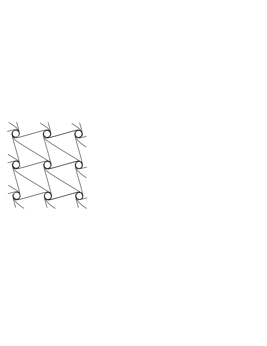
We have indicated the lamination $\widetilde{\lambda}$ in this cover, which is obtained from a standard triangulation by spinning leftward around the boundary components. The projection of this to $Y$ is $\lambda$. This discussion applies equally well when $Y$ has ends that are cusps of $S$. In this case the leaves that we drew as winding around $\partial Y$ simply go out the corresponding cusp.

Let $g\in\operatorname{\mathbf{pleat}}_{\rho}(P_{0}\cap P_{1})$ be the pleated surface mapping $\lambda$ geodesically. An inspection of the diagram gives this bound on the alternation numbers:

$$a(\lambda,\alpha_{i})\leq 4$$

for $i=0,1$ (in fact it is 2 when $Y$ is a one-holed torus and $4$ when $Y$ is a four-holed sphere). And furthermore that $\alpha_{0}$ and $\alpha_{1}$ cross no closed leaves of $\lambda$. Efficiency of Pleated Surfaces then gives us the inequality

$$\ell_{\sigma_{g}}(\alpha_{i})\leq\ell_{\rho}(\alpha_{i})+C$$

for $i=0,1$ and a uniform $C$. Thus $g\in\operatorname{\mathbf{good}}_{\rho}(P_{i},C)$ for $i=0,1$, and the lemma is proved. ∎

The following lemma controls the geometry of a halfway surface. It will be instrumental in the last part of the proof of the main theorem.

Lemma 4.3.

Let $P_{0}\to P_{1}$ be an elementary move exchanging $\alpha$ and $\alpha^{\prime}$, and let $g\in\operatorname{\mathbf{good}}_{\rho}(P_{0},C_{1})\cap\operatorname{\mathbf{good}}_{\rho}(P_{1},C_{1})$. Assume that $\alpha$ and $\alpha^{\prime}$ are realized as geodesics in $\sigma_{g}$, and suppose that

$$\ell_{\rho}(\alpha)<\epsilon_{1}/2$$

but

$$\ell_{\sigma_{g}}(\alpha)\geq\epsilon_{1}.$$

Then there is an upper bound $C_{2}$, depending only on $\epsilon_{1},C_{1}$ and the topological type of $S$, so that

$$l_{\sigma_{g}}(a)\leq C_{2}$$

for each arc $a$ of $\alpha^{\prime}\cap\operatorname{\mathbf{collar}}(\alpha,\sigma_{g})$.

Proof.

Let $a$ be an arc of $\alpha^{\prime}\cap\operatorname{\mathbf{collar}}(\alpha,\sigma_{g})$ – there may be one or two such arcs. Let $L=l_{\sigma_{g}}(a)=l_{N}(g(a))$. Deform $a$ fixing endpoints to a path $q_{0}*a^{\prime}*q_{1}$ with $q_{i}$ orthgonal paths from $\partial a$ to $\alpha$, and $a^{\prime}$ running along $\alpha$. The lengths of $q_{i}$ are at most $w(\epsilon_{0})$, and $l(a^{\prime})\leq L$. Lemma 8.4 allows us to deform $g(a^{\prime})$, fixing endpoints, to $p_{0}*a^{\prime\prime}*p_{1}$ with $l_{N}(p_{i})\leq a_{1}$ and $a^{\prime\prime}$ in the $\epsilon_{1}/2$-Margulis tube of $\alpha$, so that

$$l_{N}(a^{\prime\prime})=n\epsilon_{1}/2+r^{\prime}$$

where we write $l(a^{\prime})=n\ell_{\sigma_{g}}(\alpha)+r$, $n\in{\mathbb{Z}}_{\geq 0}$, $r\in[0,\ell_{\sigma_{g}}(\alpha)]$, and $|r-r^{\prime}|\leq a_{2}$. Since $\ell_{\sigma_{g}}(\alpha)\geq\epsilon_{1}$, we conclude that $g(a)$ can be deformed to an arc $a^{\prime\prime\prime}=g(q_{0})*p_{0}*a^{\prime\prime}*p_{1}*g(q_{1})$, so that

$$l_{N}(a^{\prime\prime\prime})\leq{\textstyle{\frac{1}{2}}}L+c$$ (4.3)

with $c$ depending on the previous constants. This is shorter than $g(a)$ by at least $L/2-c$, so we can shorten the curve $g(\alpha^{\prime})$ by at least this much, concluding that

$$\ell_{\rho}(\alpha^{\prime})\leq\ell_{\sigma_{g}}(\alpha^{\prime})-{\textstyle{\frac{1}{2}}}L+c.$$

On the other hand $\ell_{\sigma_{g}}(\alpha^{\prime})-C_{1}\leq\ell_{\rho}(\alpha^{\prime})$ since $g\in\operatorname{\mathbf{good}}_{\rho}(\alpha^{\prime},C_{1})$, so we obtain an upper bound on $L$. ∎

5. Resolution sequences

In Masur-Minsky [37], we show the existence of special sequences of elementary moves that are controlled in terms of the geometry of the complex of curves, and particularly the projections $\pi_{Y}$. First some terminology: if $P_{0}\to P_{1}\to\cdots\to P_{n}$ is an elementary-move sequence and $\beta$ is any vertex of ${\mathcal{C}}(S)$, we denote

$$J_{\beta}=\{j\in[0,n]:\beta\in P_{j}\}.$$

Note that if $J_{\beta}$ is an interval $[k,l]$, then the elementary move $P_{k-1}\to P_{k}$ exchanges some $\alpha$ for $\beta$, and $P_{l}\to P_{l+1}$ exchanges $\beta$ for some $\alpha^{\prime}$. Both $\alpha$ and $\alpha^{\prime}$ intersect $\beta$, and we call them the predecessor and successor of $\beta$, respectively.

In the following theorem, where $\beta_{0},\ldots,\beta_{m}$ is a sequence of vertices in ${\mathcal{C}}(S)$ we use the notation

$$J_{[s,t]}\equiv\bigcup_{i=s}^{t}J_{\beta_{i}}.$$

Theorem 5.1.

(Controlled Resolution Sequences)  Let $P$ and $Q$ be maximal curve systems in $S$. There exists a geodesic in ${\mathcal{C}}_{1}(S)$ with vertex sequence $\beta_{0},\ldots,\beta_{m}$, and an elementary move sequence $P_{0}\to\ldots\to P_{n}$, with the following properties:

1. $\beta_{0}\in P_{0}=P$ and $\beta_{m}\in P_{n}=Q$.

2. Each $P_{j}$ contains some $\beta_{i}$.

3. $J_{\beta}$, if nonempty, is always an interval, and if $[s,t]\subset[0,m]$ then

   $$|J_{[s,t]}|\leq K(t-s)\sup_{Y}d_{Y}(P,Q)^{a},$$

   where the supremum is over only those non-annular subsurfaces $Y$ whose boundary curves are components of some $P_{k}$ with $k\in J_{[s,t]}$.

4. If $\beta$ is a curve with non-empty $J_{\beta}$, then its predecessor and successor curves $\alpha$ and $\alpha^{\prime}$ satisfy

   $$|d_{\beta}(\alpha,\alpha^{\prime})-d_{\beta}(P,Q)|\leq\delta.$$

The constants $K,a,\delta$ depend only on the topological type of $S$. The expression $|J|$ for an interval $J$ denotes its diameter.

The sequence $\{P_{i}\}$ in this theorem is called a resolution sequence. Such sequences are constructed in [37], using what we call “hierarchies of geodesics” in ${\mathcal{C}}(S)$. The machinery of [37] is cumbersome to describe fully, so we will give just a rough description of the construction and an indication of how the results of [37] imply Theorem 5.1.

The construction is by an inductive procedure: we begin with what we call a “tight geodesic”, which is a sequence $m_{i}$ of simplices in ${\mathcal{C}}(S)$ with the first in $P$ and the last in $Q$, so that any sequence $\beta_{i}\in m_{i}$ of vertices yields a geodesic in ${\mathcal{C}}_{1}(S)$ joining $P$ to $Q$. (The $m_{i}$ satisfy an additional condition which we need not use here). The link of each $m_{i}$ is itself a curve complex for a subsurface, in which $m_{i-1}$ and $m_{i+1}$ represent two simplices, and we construct a geodesic connecting them. We then repeat, with the complexity of the subsurfaces decreasing at each step. (The actual construction is considerably complicated by the need to take care of endpoints of geodesics correctly, and by the fact that a typical simplex cuts up the surface into several components, in each of which the construction continues independently). The final structure is a collection of geodesics in subsurfaces related by inclusion, and the pants decompositions $P_{k}$ are obtained by taking “slices”: picking a vertex at one level and then inductively adding vertices from the geodesics supported in its complementary subsurfaces. These slices can be “resolved” into the sequence described in Theorem 5.1, where the elementary moves $P_{k}\to P_{k+1}$ correspond to steps along geodesics in highest-level subsurfaces, which are always one-holed tori or four-holed spheres.

The fact that $J_{\beta}$ is always an interval follows from the proof of Proposition 5.4 in [37], in the course of which we establish a monotonicity property of the way a resolution steps through the geodesics in a hierarchy, that implies no curve is ever repeated once it has been traversed.

To obtain the inequality in part (3), note first that the length of $J_{[s,t]}$ is just the sum of the lengths of the geodesics in the highest level subsurfaces meeting the slices based at $\beta_{s},\ldots,\beta_{t}$. Each of these subsurfaces arises from vertices in a lower-level (higher complexity) subsurface, so their number is bounded by the sum of the lengths of the geodesics at the lower level. Continuing inductively, if we have a length bound of $B$ on all the geodesics encountered (and a length $(t-s)$ at the bottom level), we obtain a bound of the form $K(t-s)B^{a}$, where $a$ bounds the number of levels, which only depends on the topological complexity of $S$.

Finally, the length of a geodesic supported in a subsurface $Y$ is bounded by a multiple of the projection distance $d_{Y}(P,Q)$: this is the substance of Lemma 6.2 of [37], which involves a crucial use of the hyperbolicity property of ${\mathcal{C}}(S)$, from [36]. The bound of part (3) follows.

Part (4) follows from the same construction, which in fact includes annuli and their arc complexes as part of the discussion. The bound is just a restatement of Lemma 6.2 of [37] applied to annuli.

6. The bounded shear lemma

In this section we will develop some estimates of shearing in annuli that will be used near the end of the proof of the main theorem, in Section 7.

We begin with an observation. Let $\sigma$ be a hyperbolic metric on $S$, $\gamma$ a simple geodesic in $S$, and $B=\operatorname{\mathbf{collar}}(\gamma,\sigma)$. Let $\hat{Y}$ be the compactified annular lift associated to $\gamma$ and $\hat{B}$ the annular lift of $B$ to $\hat{Y}$. Let $E$ denote one of the components of $\hat{Y}\setminus\hat{B}$.

There is only a bounded amount of twisting that a geodesic crossing $\hat{Y}$ can do in $E$. In fact, let $\beta_{1}$ and $\beta_{2}$ be any two geodesic lines connecting the two boundaries of $\hat{Y}$. We have:

$$d_{{\mathcal{A}}(E)}(\beta_{1}\cap E,\beta_{2}\cap E)\leq 4.$$ (6.1)

Figure 5. The relative twisting $d_{{\mathcal{A}}(E)}$ of $\beta_{1}\cap E$ and $\beta_{2}\cap E$ is bounded.

Proof.

The width of the collar of $\gamma$ is the function $w(\ell(\gamma))$ described in the Appendix.

Lift $\hat{B}$ to a $w$-neighborhood $\widetilde{B}$ of a geodesic lift $\Gamma$ of $\gamma$ in ${\mathbb{H}}^{2}$. For $i=1,2$, $\beta_{i}$ lifts to a geodesic arc $\widetilde{\beta}_{i}$ connecting $\partial\widetilde{B}$ to the circle at infinity. Let $p$ denote the length of its orthogonal projection to $\Gamma$. This is largest when $\widetilde{\beta}_{i}$ is tangent to $\partial\widetilde{B}$, so let us consider this case. The arcs $\widetilde{\beta}_{i}$ and its projection to $\Gamma$ form opposite sides of a quadrilateral with three right angles and an ideal vertex, whose two finite sides have lengths $w$ and $p$ (see Figure 6). Hyperbolic trigonometry (Buser [12, 2.3.1(i)]) gives us

$$\sinh(w)\sinh(p)=1.$$

On the other hand we have from the definitions in §8 that $w=\max(w_{0}/2,w_{0}-1)$ where $w_{0}$ satisfies

$$\sinh(w_{0})\sinh(\ell/2)=1.$$

From this we obtain an expression for $p/\ell$ as a function of $w_{0}$, and one can deduce that this quantity is bounded. Indeed the maximum is obtained at $w_{0}=2$, and we have

$$\frac{p}{\ell}<1.5$$

In other words, $\beta_{i}\cap E$ travels less than 1.5 times around the annulus, as measured by its orthogonal projection. We deduce that $\beta_{1}$ and $\beta_{2}$ intersect at most 3 times in $E$. The bound (6.1) follows. ∎

Figure 6. The quadrilateral formed by $\widetilde{\beta}_{i}$ and its projection to the lift of $\gamma$

This observation prompts us to define the following measure of shearing of two different metrics outside a collar. Let $\sigma,\tau$ be two hyperbolic metrics on $S$ and let $B$ be an annulus which is equal to both $\operatorname{\mathbf{collar}}(\gamma,\sigma)$ and $\operatorname{\mathbf{collar}}(\gamma,\tau)$. Lift to $\hat{B}$ in $\hat{Y}$ as above. We let the shear outside $B$ of the two metrics be the quantity

$$\sup_{E,\alpha_{\sigma},\alpha_{\tau}}d_{{\mathcal{A}}(E)}(\alpha_{\sigma}\cap E,\alpha_{\tau}\cap E).$$

Here $E$ varies over the two complementary annuli of $\hat{B}$ in $\hat{Y}$, $\alpha_{\sigma}$ varies over all $\sigma$-geodesics that connect the two boundaries, and $\alpha_{\tau}$ varies over all $\tau$-geodesics that connect the two boundaries. Note that the shear depends on the pointwise metrics, and not just their isotopy classes.

The point of having a bound on this shear is that it allows us to measure twisting by restricting to a collar. That is, suppose in the setting above the shear outside $B$ is bounded by $D$. Then if $\alpha_{\sigma}$ and $\alpha_{\tau}$ are any two $\sigma$ and $\tau$ geodesics, respectively, which cross $\gamma$, we immediately have

$$|d_{{\mathcal{A}}(B)}(\alpha_{\sigma}\cap B,\alpha_{\tau}\cap B)-d_{\gamma}(\alpha_{\sigma},\alpha_{\tau})|\leq 2D.$$ (6.2)

Note that $d_{{\mathcal{A}}(B)}$ is a measure of twisting inside the collar which depends on the particular curves we chose, whereas $d_{\gamma}$ depends only on homotopy classes.

The main lemma of this section bounds the shear outside a collar for pairs of metrics satisfying a special condition.

Lemma 6.1.

(Shear bound)  Suppose $R$ is a subsurface of $S$ which is convex in two hyperbolic metrics $\sigma$ and $\tau$, and that $\sigma$ and $\tau$ are locally $K$-bilipschitz in the complement of $R$. Suppose that one component of $R$ is an annulus $B$ which is equal to both $\operatorname{\mathbf{collar}}(\gamma,\sigma)$ and $\operatorname{\mathbf{collar}}(\gamma,\tau)$ for a certain curve $\gamma$.

Figure 7. $\hat{Y}$, seen in the metric $\hat{\sigma}$ on top, and the metric $\hat{\tau}$ on the bottom. Some components of $\hat{R}$ are shown, shaded.

Then the shear outside $B$ of $\sigma$ and $\tau$ is bounded above by $\delta_{0}K$, where $\delta_{0}$ depends only on the topological type of $S$.

Proof.

Let $\hat{Y}$ be the compactified annular lift, and let $\hat{\sigma}$ and $\hat{\tau}$ be the lifts of $\sigma$ and $\tau$ to $\hat{Y}$. Let $\hat{R}$ denote the lift of $R$ to $\hat{Y}$, and let $\hat{B}$ be the component of $\hat{R}$ which is a homeomorphic lift of $B$. Let $E$ be one of the components of $\hat{Y}\setminus\hat{B}$. There is a uniform upper bound $b$ to the $\hat{\sigma}$-length of the shortest arc $\alpha$ connecting $\hat{B}$ to any component $D$ of $\hat{R}$ contained in $E$. This comes from a standard area bound: Since $\ell_{\sigma}(\partial B)$ is bounded below by $b_{0}$ (see §8), an embedded collar of radius $r$ around $B$ has area at least $b_{0}r$. Since the area of $S$ is fixed by the Gauss-Bonnet theorem, $r$ is uniformly bounded. The first self-tangency of this collar yields a bound for $b$.

Since by (6.1) the choice of $\alpha_{\sigma}$ cannot change the twisting number in the lemma by more than 4, we may assume that $\alpha_{\sigma}\cap E$ has an initial segment which is this shortest arc $\alpha$. Similarly we may assume that $\alpha_{\tau}$ is orthogonal to $\partial B$ in the metric $\tau$. The Lipschitz condition in the complement of $R$ implies that the $\hat{\tau}$-length of $\alpha$ is bounded by $Kb$. Thus the number of essential intersections that $\alpha_{\tau}$ can have with $\alpha_{\sigma}$ in the interval $\alpha$ is bounded by $Kb/b_{0}$, since between any two such there is a segment of $\alpha$ that projects orthogonally (in $\hat{\tau}$) to an entire boundary component of $B$. The remainder of $\alpha_{\sigma}$ is contained in a convex set whose boundary $\xi$ is the lift of a boundary component of $R$. Since $R$ is a convex subsurface both in $\sigma$ and $\tau$, $\xi$ still bounds a convex set in the metric $\hat{\tau}$. Thus $\alpha_{\tau}$ can have at most one essential intersection with $\alpha_{\sigma}$ in this convex set. ∎

7. The proof of the main theorem

As discussed in the outline, after [47] it suffices to prove this direction of the theorem:

$$\sup_{Y}d_{Y}(\nu_{+},\nu_{-})<K\quad\implies\quad\inf_{\gamma}\ell_{\rho}(\gamma)>\epsilon$$

for $\epsilon$ depending only on $K$ and $S$, with the infimum over $\gamma$ that are not externally short.

For simplicity of exposition, let us first prove the theorem in the case when both ends of $N_{\rho}$ are degenerate. At the end of the section we will indicate the changes in the argument necessary if one or both of the ends are geometrically finite.

Let $K_{1}$ be a constant to be determined shortly, and let $\epsilon_{2}$ be such that a $K_{1}$-neighborhood of any $\epsilon_{2}$-Margulis tube is still contained in an $\epsilon_{1}$-Margulis tube (see §2.5).

Fix a closed curve $\gamma$ in $S$, and assume $\ell_{\rho}(\gamma)<\epsilon_{2}$. In particular $\gamma$ must be simple (§2.5), and represents a vertex of ${\mathcal{C}}_{0}(S)$. Our goal will be to bound the radius of the Margulis tube ${\mathbf{T}}_{\gamma}(\epsilon_{0})$.

Initial pants

Our first step is to obtain two pants decompositions $P_{+}$ and $P_{-}$ of moderate $\rho$-length, and pleated surfaces $f_{\pm}\in\operatorname{\mathbf{pleat}}_{\rho}(P_{\pm})$ which homologically encase ${\mathbf{T}}_{\gamma}(\epsilon_{1})$.

Lemma 7.1.

Suppose that $\rho\in{\mathcal{D}}_{\mathrm{np}}(S)$ has two degnerate ends, so that $\nu_{\pm}\in\operatorname{{\mathcal{E}}{\mathcal{L}}}(S)$.

Let ${\mathcal{U}}_{+}$ and ${\mathcal{U}}_{-}$ denote neighborhoods in $\operatorname{{\mathcal{U}}{\mathcal{M}}{\mathcal{L}}}(S)$ of $\nu_{+}$ and $\nu_{-}$, respectively. There exist pants decompositions $P_{+}$ and $P_{-}$ lying in ${\mathcal{U}}_{+}$ and ${\mathcal{U}}_{-}$, respectively, with the following properties:

1. $\ell_{\rho}(P_{\pm})\leq L_{1}$

2. Given $f_{+}\in\operatorname{\mathbf{pleat}}_{\rho}(P_{+})$ and $f_{-}\in\operatorname{\mathbf{pleat}}_{\rho}(P_{-})$, ${\mathbf{T}}_{\gamma}(\epsilon_{1})$ is homologically encased by $f_{+}$ and $f_{-}$.

The last statement in the lemma means that ${\mathbf{T}}_{\gamma}(\epsilon_{1})$ is covered with degree 1 by any 3-chain whose boundary relative the cusps is $f_{+}-f_{-}$. In particular, any proper homotopy from $f_{+}$ to $f_{-}$ must cover all of ${\mathbf{T}}_{\gamma}(\epsilon_{1})$.

Proof.

Since the $e_{+}$ end is degenerate, there is a sequence of pleated surfaces $f^{+}_{i}$ eventually contained in every neighborhood of the end. Choose $P^{+}_{i}\in\operatorname{\mathbf{short}}(\sigma_{f^{+}_{i}})$. Then the geodesic representatives of $P^{+}_{i}$ must also eventually exit $e_{+}$. In particular they must converge to $\nu_{+}$ in $\operatorname{{\mathcal{U}}{\mathcal{M}}{\mathcal{L}}}$. The same discussion applies with $+$ replaced by $-$.

Since $(N_{\rho},cusps)$ is homeomorphic to $(S\times{\mathbb{R}},cusps\times{\mathbb{R}})$ and ${\mathbf{T}}_{\gamma}(\epsilon_{1})$ is compact, any pleated surface in the proper homotopy class of $\rho$ which is sufficiently far in a neighborhood of $e_{+}$ (or $e_{-}$) can be deformed to infinity, through cusp-preserving maps, without meeting ${\mathbf{T}}_{\gamma}(\epsilon_{1})$.

Choosing $i$ high enough, then, insures that $f^{+}_{i}$ and $f^{-}_{i}$ homologically encase ${\mathbf{T}}_{\gamma}(\epsilon_{1})$ and that $P^{\pm}_{i}\in{\mathcal{U}}_{\pm}$. Furthermore $P^{\pm}_{i}\in\operatorname{\mathbf{short}}(\sigma_{f^{+}_{i}})$ implies that $f^{\pm}_{i}\in\operatorname{\mathbf{good}}_{\rho}(P^{\pm}_{i},L_{1})$, so that by Lemma 4.1 there is a $K$-good homotopy (with $K$ depending on $L_{1}$) between $f^{\pm}_{i}$ and any map in $\operatorname{\mathbf{pleat}}(P^{\pm}_{i})$. This homotopy has bounded tracks outside the Margulis tubes of $P^{\pm}_{i}$, if any. Thus we may choose $i$ high enough that this homotopy also avoids ${\mathbf{T}}_{\gamma}(\epsilon_{1})$, so that $P_{\pm}=P^{\pm}_{i}$ satisfies the conclusions of the lemma. ∎

Resolution sequence and block map

Join $P_{+}$ to $P_{-}$ with a resolution sequence $P_{-}=P_{0}\to\cdots\to P_{n}=P_{+}$, as in Theorem 5.1. Let $\{\beta_{i}\}_{i=0}^{m}$ be the vertex sequence of the associated geodesic in ${\mathcal{C}}(S)$.

Define a map $H:S\times[0,n]\to N_{\rho}$ as follows. For each $j=0,\ldots,n$ choose $g_{j}\in\operatorname{\mathbf{pleat}}_{\rho}(P_{j})$, and for $j=0,\ldots,n-1$ let $g_{j+\frac{1}{2}}$ be a map in $\operatorname{\mathbf{good}}_{\rho}(P_{j},C_{1})\cap\operatorname{\mathbf{good}}_{\rho}(P_{j+1},C_{1})$, promised to exist by Lemma 4.2.

Lemma 4.1 gives us a constant $K_{1}$ so that $g_{j}$ and $g_{j+\frac{1}{2}}$ admit a $K_{1}$-good homotopy, and so do $g_{j+\frac{1}{2}}$ and $g_{j+1}$. Let $H|_{S\times[j,j+\frac{1}{2}]}$ and $H|_{S\times[j+\frac{1}{2},j+1]}$ be these two homotopies. Up to suitable precomposition by homeomorphisms of $S$ isotopic to the identity, we can arrange for the definitions to agree on each integer and half-integer level, so they may be concatenated to yield a single map $H$. The constant $K_{1}$ described here gives us our choice of $\epsilon_{2}$, which we note depends only on the topological type of $S$.

Let $\sigma(u)=\sigma_{H_{u}}$ be the induced metric on $S\times\{u\}$, which we note is hyperbolic for $u$ an integer or half-integer. We endow $S\times[0,n]$ with the metric that restricts to $\sigma(u)$ in the horizontal direction and to the induced metric from ${\mathbb{R}}$ in the vertical direction, and such that the two directions are orthogonal.

Restricting the block map

Assuming the neighborhoods ${\mathcal{U}}_{\pm}$ have been chosen sufficiently small, we can throw away all but a bounded number of the blocks and still have the encasing condition. To see this, begin with the following claim:

Claim 7.2.

There is a constant $C_{2}$ depending only on the topological type of $S$, and a subinterval $I_{\gamma}\subseteq[0,m]$ of diameter at most $C_{2}$, so that $H(S\times[j,j+1])$ can meet ${\mathbf{T}}_{\gamma}(\epsilon_{2})$ only if $j$ or $j+1$ are in $J_{I_{\gamma}}$.

(The notation $J_{I}$ is defined in §5.)

Proof.

Let $\beta_{i}$ be a vertex that is in $P_{j}$. If $H(S\times\{j\})$ meets ${\mathbf{T}}_{\gamma}(\epsilon_{1})$ then (see §2.5) $\ell_{\sigma(j)}(\gamma)\leq\epsilon_{0}$, and in particular

$$\gamma\in\operatorname{\mathbf{short}}(\sigma(j))\subset\Pi_{\rho}(\beta_{i}).$$

It follows from Lemma 3.1 that

$$d_{\mathcal{C}}(\beta_{i},\gamma)\leq C$$

where $C$ depends only on the topological type of $S$. Thus, since $\{\beta_{0},\ldots,\beta_{m}\}$ are the vertices of a geodesic, the possible values of $i$ lie in an interval of diameter at most $2C$, which we call $I_{\gamma}$. In other words, $j\in J_{I_{\gamma}}$.

It remains to notice that, by the choice of $\epsilon_{2}$ and the $K_{1}$-good homotopy property, if any part of a block $H(S\times[j,j+1])$ meets ${\mathbf{T}}_{\gamma}(\epsilon_{2})$ then one of the boundaries must meet ${\mathbf{T}}_{\gamma}(\epsilon_{1})$, and hence $j$ or $j+1$ are in $J_{I_{\gamma}}$. ∎

Let us therefore restrict our elementary move sequence to

$$P_{s-1}\to\cdots\to P_{t+1}$$

where $[s,t]=J_{I_{\gamma}}$. This subsequence must still encase ${\mathbf{T}}_{\gamma}(\epsilon_{2})$, since we have thrown away only blocks that avoid ${\mathbf{T}}_{\gamma}(\epsilon_{2})$. Let $M=t-s=|J_{I_{\gamma}}|$.

In order to deduce a bound on $M$ from the diameter bound on $I_{\gamma}$, we consider part (3) of Theorem 5.1, which tells us that

$$M\leq K(2C)\sup_{Y}d_{Y}(P_{+},P_{-})^{a},$$ (7.1)

where the supremum is over subsurfaces $Y$ whose boundaries appear among the $P_{j}$ in our subsequence. Such $P_{j}$ must lie in a $C+1$ neighborhood of $\gamma$, in the $d_{\mathcal{C}}$ metric. In order to compare $d_{Y}(P_{+},P_{-})$ to $d_{Y}(\nu_{+},\nu_{-})$ for such $Y$, we will need the following lemma:

Lemma 7.3.

There exists a constant $b$ depending only on $S$, so that given $\gamma\in{\mathcal{C}}_{0}(S)$, $R>0$ and $\nu\in\operatorname{{\mathcal{E}}{\mathcal{L}}}(S)$, there is a neighborhood ${\mathcal{U}}$ of $\nu$ in $\operatorname{{\mathcal{U}}{\mathcal{M}}{\mathcal{L}}}(S)$ for which the following holds:

If $Y\subset S$ is a subsurface with $d_{\mathcal{C}}(\gamma,\partial Y)\leq R$ and $\beta\in{\mathcal{C}}_{0}(S)\cap{\mathcal{U}}$, then

$$d_{Y}(\beta,\nu)\leq b.$$

Proof.

By Klarreich’s Theorem 2.1, $\operatorname{{\mathcal{E}}{\mathcal{L}}}(S)$ is naturally identified with the Gromov boundary of ${\mathcal{C}}(S)$. By the definition of the Gromov boundary, there is a neighborhood ${\mathcal{U}}$ of $\nu$ such that, if $\beta,\beta^{\prime}\in{\mathcal{C}}_{0}(S)$ are in ${\mathcal{U}}$ then any geodesic $g$ in ${\mathcal{C}}_{1}(S)$ connecting them must lie outside an $R+2$-ball of $\gamma$. In particular every vertex of $g$ must be at least distance 2 from $\partial Y$, and hence must intersect $\partial Y$ essentially. Theorem 3.1 of [37] states that in such a situation

$$\operatorname{diam}_{Y}(\pi_{Y}(g))\leq A$$

for a constant $A$ depending only on the topological type of $S$, and in particular $d_{Y}(\beta,\beta^{\prime})\leq A$.

Now consider a sequence $\beta_{i}$ converging to $\nu$ in $\operatorname{{\mathcal{U}}{\mathcal{M}}{\mathcal{L}}}(S)$, with $\beta_{0}=\beta$. After restricting to a subsequence if necessary, the $\beta_{i}$ converge in the Hausdorff topology to a lamination that includes the support of $\nu$, which means that eventually $\operatorname{diam}_{Y}(\pi_{Y}(\beta_{i})\cup\pi_{Y}(\nu))\leq 2$. Thus $d_{Y}(\beta,\nu)\leq A+2$. ∎

Thus if we choose the original neighborhoods ${\mathcal{U}}_{+}$ and ${\mathcal{U}}_{-}$ sufficiently small, this lemma gives us

$$d_{Y}(P_{+},P_{-})\leq d_{Y}(\nu_{+},\nu_{-})+2b.$$ (7.2)

The hypothesis of the main theorem bounds the right side, so together with (7.1) we obtain our desired uniform bound on $M$.

Suppose that $\gamma$ is not a component of any $P_{j}$. Then according to Lemma 4.1, each block $H|_{S\times[j,j+1]}$ has track lengths of at most $2K_{1}$ within ${\mathbf{T}}_{\gamma}(\epsilon_{1})$. There are only $M+2$ blocks in our restricted sequence, and they cover all of ${\mathbf{T}}_{\gamma}(\epsilon_{1})$. The beginning and the end of the sequence are outside of ${\mathbf{T}}_{\gamma}(\epsilon_{1})$, so that any point in ${\mathbf{T}}_{\gamma}(\epsilon_{1})$ is at most

$$2K_{1}(M+2)$$

from its boundary. This bounds the radius of ${\mathbf{T}}_{\gamma}(\epsilon_{1})$ by $2K_{1}(M+2)$, and a corresponding lower bound for $\ell_{\rho}(\gamma)$ follows as in §2.5.

Bounding twists

Now suppose that $\gamma$ does appear among the $\{P_{j}\}$. Then $J_{\gamma}$ is some nonempty subinterval of $J_{I_{\gamma}}$ by Theorem 5.1, and we let $\alpha$ and $\alpha^{\prime}$ be the predecessor and successor curves to $\gamma$ in the sequence. Both of them cross $\gamma$, and we have by part (4) of Theorem 5.1 that $d_{\gamma}(\alpha,\alpha^{\prime})$ is uniformly approximated by $d_{\gamma}(P_{+},P_{-})$, which by (7.2) and the hypothesis of the main theorem, is uniformly bounded. Let $D$ denote this bound.

Write $J_{\gamma}=[k,l]$. By the normalization used in Lemma 4.1, for all integer and half-integer $u\in[k,l]$ the annuli $\operatorname{\mathbf{collar}}(\gamma,\sigma(u))$ coincide. Name this common annulus $B$. consider the solid torus

$$U=B\times[k-{\textstyle{\frac{1}{2}}},l+{\textstyle{\frac{1}{2}}}].$$

The map $H$ can take the complement of $U$ at most $2K_{1}(M+2)$ into ${\mathbf{T}}_{\gamma}(\epsilon_{1})$, by the same argument as above, and hence there is a uniform $\epsilon_{3}>0$ so that $H(U)$ must cover ${\mathbf{T}}_{\gamma}(\epsilon_{3})$. Assume $\ell_{\rho}(\gamma)<\epsilon_{3}$, for otherwise we are done.

Consider the geometry of $\partial U$, in the metric we have placed on $S\times[0,n]$. The top annulus $B\times\{k-{\textstyle{\frac{1}{2}}}\}$ is $\operatorname{\mathbf{collar}}(\gamma,\sigma({k-{\textstyle{\frac{1}{2}}}}))$. Since $H_{k-\frac{1}{2}}\in\operatorname{\mathbf{good}}(\gamma,C_{1})$ by construction, we have an upper bound of $\epsilon_{3}+C_{1}$ on the circumference of this collar. We also have a lower bound of $\epsilon_{3}$ since the image of $H_{k-\frac{1}{2}}$ avoids the interior of ${\mathbf{T}}_{\gamma}(\epsilon_{3})$. Thus, this annulus has uniformly bounded geometry. The same holds for $B\times\{l+{\textstyle{\frac{1}{2}}}\}$ in the metric $\sigma({l+{\textstyle{\frac{1}{2}}}})$

The vertical annuli $\partial B\times[k-{\textstyle{\frac{1}{2}}},l+{\textstyle{\frac{1}{2}}}]$ have height bounded by $M+1$. Thus $\partial U$ is a concatenation of four annuli of bounded geometry, and hence is itself up to uniformly bounded distortion a Euclidean square torus, and $H$ maps it with a uniform Lipschitz constant into $N$. Let us now try to control a meridian curve for $U$.

Realize $\alpha$ as a geodesic in $\sigma({k-{\textstyle{\frac{1}{2}}}})$ and let $a$ be an arc of $\alpha\cap B$ (there may be two). Similarly assume $\alpha^{\prime}$ is a geodesic in $\sigma({l+{\textstyle{\frac{1}{2}}}})$ and let $a^{\prime}$ be an arc of $\alpha^{\prime}\cap B$. Lemma 4.3 gives an upper bound for the length of $a$ in $\sigma({k-{\textstyle{\frac{1}{2}}}})$, and for the length of $a^{\prime}$ in $\sigma({l+{\textstyle{\frac{1}{2}}}})$. The curve

$$m=\partial(a\times[k-{\textstyle{\frac{1}{2}}},l+{\textstyle{\frac{1}{2}}}]),$$

is a meridian of $U$, and we claim that its length is uniformly bounded.

The arc $a$ may a priori be long in $\sigma({l+{\textstyle{\frac{1}{2}}}})$, but its length is estimated by the number of times it twists around the annulus, which in turn is estimated by $d_{{\mathcal{A}}(B)}(a,a^{\prime})$ since $a^{\prime}$ has bounded length in this metric.

We can bound this twisting using the results in Section 6. Note first that, for each $j=k-{\textstyle{\frac{1}{2}}},k,\ldots,l-{\textstyle{\frac{1}{2}}},l$, the pair of metrics $\sigma(j),\sigma({j+{\textstyle{\frac{1}{2}}}})$ satisfy the hypotheses of Lemma 6.1. That is, they are $K_{1}$-bilipschitz outside a union of collars including $B$. Thus, Lemma 6.1 bounds the shearing outside $B$ at each step, and the number of steps is bounded by $2M+2$. We conclude that there is a bound on the shearing outside $B$ of the two metrics $\sigma(k-{\textstyle{\frac{1}{2}}})$ and $\sigma(l+{\textstyle{\frac{1}{2}}})$. It follows as in (6.2) that we have a bound of the form

$$|d_{{\mathcal{A}}(B)}(a,a^{\prime})-d_{\gamma}(\alpha,\alpha^{\prime})|\leq M^{\prime}$$ (7.3)

With this estimate and the bound $d_{\gamma}(\alpha,\alpha^{\prime})\leq D$, we find that $a$ and $a^{\prime}$ intersect a bounded number of times, so that the length of $a$ is uniformly bounded in $S\times\{l+{\textstyle{\frac{1}{2}}}\}$. It follows that $H(m)$ is uniformly bounded. It therefore spans a disk of bounded diameter, and now by a coning argument we can homotope $H$ on all of $U$ to a new map of bounded diameter. This bounds the radius of ${\mathbf{T}}_{\gamma}(\epsilon_{3})$ from above, and again we are done.

The case of geometrically finite ends

The main change in the argument comes at the beginning, in our choice of $P_{+}$ and $P_{-}$.

Suppose that $e_{+}$ is geometrically finite. It suffices to consider $\gamma$ which is not externally short, i.e. $\ell_{\nu_{+}}(\gamma)>\epsilon_{0}$, because the second statement in the main theorem considers only such curves, and the first statement is insensitive to the removal of a finite number of curves from consideration. The choice of $\epsilon_{1}$ and Sullivan’s theorem (see §2.5) imply that we also have $\ell_{\nu^{\prime}_{+}}(\gamma)>\epsilon_{1}$.

We may therefore choose a pants decomposition $P_{+}\in\operatorname{\mathbf{short}}(\nu^{\prime}_{+})$ so that $\gamma$ is not one of its components (our choice of $L_{1}$ was made so that this would be possible, see §2.6). Let $f^{\prime}_{+}:S\to\partial_{+}(C(N_{\rho}))$ be the pleated surface in the homotopy class of $\rho$ that parametrizes the $e_{+}$-boundary of the convex hull. In particular $f^{\prime}_{+}\in\operatorname{\mathbf{good}}_{\rho}(P_{+},L_{1})$. Thus, choosing $f_{+}\in\operatorname{\mathbf{pleat}}_{\rho}(P_{+})$, Lemma 4.1 gives us a $K_{2}$-good homotopy $G_{+}$ between $f^{\prime}_{+}$ and $f_{+}$, with $K_{2}$ depending on $L_{1}$. Since $\gamma$ is not a component of $P_{+}$, $G_{+}$ can only penetrate a distance $K_{2}$ into ${\mathbf{T}}_{\gamma}(\epsilon_{1})$, and hence does not meet ${\mathbf{T}}_{\gamma}(\epsilon_{4})$, with $\epsilon_{4}$ depending only on $K_{2}$.

We do the same thing with $f_{-},P_{-}$ if $e_{-}$ is geometrically finite, or we repeat the original discussion if $e_{-}$ is degenerate. Thus we have $f_{+},f_{-}$ encasing ${\mathbf{T}}_{\gamma}(\epsilon_{4})$.

We can therefore continue as before, constructing a resolution sequence from $P_{-}$ to $P_{+}$ and then restricting it. The argument goes through with slightly altered constants (since we have replaced $\epsilon_{1}$ with $\epsilon_{4}$), and the one step that needs attention is the comparison (7.2) between $d_{Y}(P_{+},P_{-})$ and $d_{Y}(\nu_{+},\nu_{-})$, for appropriate $Y$. In other words we must bound

$$d_{Y}(P_{+},\nu_{+})$$

in the geometrically finite case (and similarly for $e_{-}$). This quantity by definition is just $\min_{Q_{+}}d_{Y}(P_{+},Q_{+})$ where $Q_{+}$ varies over pants decompositions in $\operatorname{\mathbf{short}}(\nu_{+})$, provided $P_{+}$ meets $Y$ nontrivially and $Q_{+}$ can be found which does the same.

Since $\nu_{+}$ and $\nu^{\prime}_{+}$ admit a $K_{0}$-bilipschitz map by Sullivan’s theorem (§2.1), the $\nu^{\prime}_{+}$-length of $Q_{+}$ is bounded by $K_{0}L_{1}$, which gives a bound on its intersection number with $P_{+}$. This bounds $d_{Y}(P_{+},Q_{+})$ provided both pants decompositions intersect $Y$.

If $Y$ is not an annulus (and recall that we never consider three-holed spheres), then it automatically intersects any pants decomposition. Thus the only problematic case is if $Y$ is an annulus whose core is a component of $P_{+}$ or $Q_{+}$. However, we recall that the only annulus that actually comes into the argument is the annulus with core $\gamma$. Since $\gamma$ is not externally short, we have already chosen $P_{+}$ so that $\gamma$ is not a component of it, and we can do the same for $Q_{+}$.

The rest of the proof goes through in the same way. ∎

8. Appendix: Hyperbolic geometry

In this appendix we write out statements, and sketch some proofs, of a few facts and constructions in hyperbolic geometry. These are “well-known” in the sense that those working in this field are familiar at least with some variation of them, or would find it straightforward to derive them. Still it seems advisable to include some discussion.

Throughout, a hyperbolic surface always means a finite area hyperbolic surface which could have closed geodesic boundary components and/or cusps. By abuse of notation we usually think of a cusp as a boundary component of length 0.

Collars

Let $w_{0}$ be the function

$$w_{0}(t)=\sinh^{-1}\left(\frac{1}{\sinh\left(t/2\right)}\right).$$

For a simple closed geodesic $\gamma$ of length $\ell$ in a hyperbolic surface $X$, we define

$$\operatorname{\mathbf{collar}}_{0}(\gamma,X)=\{p\in X:\operatorname{dist}(p,\gamma)\leq w_{0}(\ell)\}.$$

When the ambient surface $X$ is understood we omit it from the notation. This set is always an embedded annulus, and in fact if $\gamma_{1}\ldots,\gamma_{k}$ are disjoint and homotopically distinct then $\operatorname{\mathbf{collar}}_{0}(\gamma_{i})$ are pairwise disjoint. (See e.g. Buser [12, Chapter 4].)

We will need a slightly smaller collar, so as to guarantee a definite amount of space in its complement. Define

$$w=\max(w_{0}/2,w_{0}-1)$$

and let

$$\operatorname{\mathbf{collar}}(\gamma,X)=\{p\in X:\operatorname{dist}(p,\gamma)\leq w(\ell)\}.$$

Let $\gamma^{\prime}_{0}$ be a boundary component of $\operatorname{\mathbf{collar}}_{0}(\gamma)$ (assume $\gamma^{\prime}_{0}\neq\gamma$ if $\gamma$ itself is in $\partial X$), and similarly let $\gamma^{\prime}\neq\gamma$ be a boundary component of $\operatorname{\mathbf{collar}}(\gamma)$. The length of $\gamma^{\prime}_{0}$ (resp. $\gamma^{\prime}$) is given by $\ell\cosh(w_{0}(\ell))$ (resp. $\ell\cosh(w(\ell))$). A bit of arithmetic shows that

$$l(\gamma^{\prime})\leq l(\gamma^{\prime}_{0})\leq\ell(\gamma)+2$$ (8.1)

We can define $\operatorname{\mathbf{collar}}_{0}(\gamma)$ and $\operatorname{\mathbf{collar}}(\gamma)$ also when $\gamma$ represents a cusp of $X$, describing them either explicitly or as a limit as $\ell\to 0$. The boundary of $\operatorname{\mathbf{collar}}_{0}(\gamma)$ for a cusp is horocyclic, and its length is 2 (the limiting value of $\ell\cosh(w_{0}(\ell))$ as $\ell\to 0$). The slightly smaller $\operatorname{\mathbf{collar}}(\gamma)$ has horocylic boundary a distance 1 inside the boundary of $\operatorname{\mathbf{collar}}_{0}(\gamma)$, so its length is $2/e$.

We remark in fact that the boundary length $\ell\cosh w_{0}(\ell)$ of $\operatorname{\mathbf{collar}}_{0}(\gamma)$ is increasing with $\ell$, and hence always at least 2. There is a similar lower bound $b_{0}$ for the boundary of $\operatorname{\mathbf{collar}}(\gamma)$, which we will not compute explicitly.

If $P=\{\gamma_{1},\ldots,\gamma_{k}\}$ is a curve system we let $\operatorname{\mathbf{collar}}(P)=\cup_{i}\operatorname{\mathbf{collar}}(\gamma_{i})$.

Hyperbolic pairs of pants

If $Y$ is a hyperbolic surface as above, with genus 0 and three boundary components, we call it a hyperbolic pair of pants. The three boundary lengths determine the metric on $Y$ completely (up to isotopy). Let $Y_{0}=Y\setminus int(\operatorname{\mathbf{collar}}(\partial Y))$.

A tripod is a copy of the 1-complex $\Delta$ obtained from three disjoint copies of $[0,1]$ (called “legs”) by identifying the three copies of $\{0\}$. The three copies of $\{1\}$ are called the boundary of $\Delta$. An essential tripod in $Y_{0}$ is an embedding of $\Delta$ (also called $\Delta$) taking $\partial\Delta$ to $\partial Y_{0}$, such that each subarc of $\Delta$ obtained by deleting one copy of $(0,1]$ is not homotopic rel endpoints into $\partial Y_{0}$ (Figure 8).

Figure 8. The two types of essential tripods

Lemma 8.1.

There is a constant $\delta>0$ such that for any hyperbolic pair of pants $Y$ and each boundary component $\gamma$ of $Y_{0}$, there is an essential tripod $\Delta\subset Y_{0}$ whose three legs have length at most $\delta$, and which meets $\gamma$.

On the other hand, there exists $\delta^{\prime}>0$ such no essential tripod in any $Y_{0}$ has all three legs of length less than $\delta^{\prime}$.

The next lemma describes how an estimate on the boundary lengths of $Y$ yields an estimate on its isometry type.

Lemma 8.2.

Given $C\geq 0$ there exists $K\geq 1$ such that the following holds.

Let $Y$ and $Y^{\prime}$ be two hyperbolic pairs of pants with boundaries $\{\gamma_{i}\}_{i=1}^{3}$ and $\{\gamma^{\prime}_{i}\}_{i=1}^{3}$, respectively. Suppose that

$$|\ell(\gamma_{i})-\ell(\gamma^{\prime}_{i})|\leq C.$$

Then there is a homeomorphism $h:int(Y)\to int(Y^{\prime})$ taking $Y_{0}$ to $Y^{\prime}_{0}$ and $\operatorname{\mathbf{collar}}(\gamma_{i})$ to $\operatorname{\mathbf{collar}}(\gamma^{\prime}_{i})$, which is $K$-bilipschitz on $Y_{0}$. Furthermore, for any arc $a$ on $\partial Y_{0}$ we have $|l(\alpha)-l(h(\alpha))|\leq K$.

Let us prove Lemma 8.2 first. Any hyperbolic pair of pants $Y$ admits a canonical decomposition into two congruent right-angled hexagons, by cutting along the shortest arcs connecting each pair of boundary components (see Buser [12]. In the limiting case of cusps we obtain degenerate hexagons with ideal vertices). Thus it will suffice to find appropriate bilipschitz maps between such hexagons.

Comparison of hexagons

Let $\Xi$ be a hyperbolic right-angled hexagon, with three alternating sides $A_{1},A_{2},A_{3}$ of lengths $a_{1},a_{2},a_{3}$. (we will adopt the convention here of denoting edges by capital letters and their lengths by the corresponding lower case letters). Each side $A_{i}$ admits an embedded “collar rectangle”, which we call $\operatorname{\mathbf{collar}}(A_{i},\Xi)$, and is just the $w(2a_{i})$-neighborhood of $A_{i}$ in $\Xi$. If $Y$ is the hyperbolic pair of pants obtained from $\Xi$ by doubling along its other three boundaries, then $\operatorname{\mathbf{collar}}(A_{i},\Xi)$ is clearly just $\operatorname{\mathbf{collar}}(\gamma_{i},Y)\cap\Xi$, where $\gamma_{i}$ is the double of $A_{i}$.

Lemma 8.2 clearly follows from the following property of hexagons:

Lemma 8.3.

Given $C>0$ there exists $K\geq 1$ so that the following holds:

Let $\Xi,\Xi^{\prime}$ be two hyperbolic right-angled hexagons with alternating sides $\{A_{i}\}$ and $\{A^{\prime}_{i}\}$, respectively. Suppose that

$$|a_{i}-a^{\prime}_{i}|\leq C,\quad i=1,2,3.$$

Then there is a label-preserving homeomorphism $f:\Xi\to\Xi^{\prime}$ which takes $\operatorname{\mathbf{collar}}(A_{i},\Xi)$ to $\operatorname{\mathbf{collar}}(A^{\prime}_{i},\Xi^{\prime})$ and is $K$-bilipschitz on the complement of the collars. Furthermore for any arc $\alpha$ in $\cup A_{i}$, we have $|l(\alpha)-l(f(\alpha))|\leq K$.

Proof.

We begin by describing a decomposition of $\Xi$ into controlled pieces in a way that is determined by the $\{a_{i}\}$. In the following, $(i,j,k)$ always denotes a permutation of $(1,2,3)$.

Case 1:

Suppose that the three “triangle inequalities”

$$a_{i}\leq a_{j}+a_{k}$$ (8.2)

all hold. Then there is a unique triple $r_{12},r_{23},r_{13}\geq 0$ satisfying

$$r_{ij}+r_{ik}=a_{i}.$$ (8.3)

(where we use the convention $r_{ij}=r_{ji}$). In fact we simply set $r_{ij}={\textstyle{\frac{1}{2}}}(a_{i}+a_{j}-a_{k})$.

Now define three “bands” $B_{ij}$ in $\Xi$ as follows: $B_{ij}$ is the (closed) $r_{ij}$-neighborhood of the edge $C_{ij}$ of $\Xi$ which is the common perpendicular of $A_{i}$ and $A_{j}$. See Figure 9.

Figure 9. The bands decomposition of $\Xi$ in case 1.

The two segments $B_{ij}\cap A_{i}$ and $B_{ik}\cap A_{i}$ cover all of $A_{i}$ and meet in their common boundary point. The interiors of $B_{ij}$ are disjoint as a consequence of the triangle inequality and the fact that $\operatorname{dist}(C_{ij},C_{ik})=a_{i}$. The closure $T$ of the complement $\Xi\setminus\bigcup_{ij}B_{ij}$ is a “triangle” with the following properties:

• Each edge $E_{ij}=T\cap B_{ij}$ has curvature $\kappa_{ij}\in[0,1]$, which is in fact given by $\tanh r_{ij}$. The curvature vector points outward.

• Adjacent edges meet at angle 0.

From this and the Gauss-Bonnet theorem we have

$$\sum_{ij=12,13,23}e_{ij}\kappa_{ij}=\pi-\mathrm{area}(T)$$

which implies the upper bound

$$e_{ij}\leq\frac{\pi}{\tanh r_{ij}}.$$ (8.4)

There is also a lower bound

$$e_{ij}\geq 2\log\frac{2}{\sqrt{3}}$$ (8.5)

obtained as follows: Extend each $E_{ij}$ to a line of constant curvature in ${\mathbb{H}}^{2}$. Each bounds a region $R_{ij}$ that contains $B_{ij}$, so that the three regions have disjoint interiors. Since $\kappa_{ij}\leq 1$, through any point $x\in\partial R_{ij}$ passes the boundary of a horoball contained in $R_{ij}$. One can check that for any three horoballs in ${\mathbb{H}}^{2}$ with disjoint interiors, and any point $p$, the distance from $p$ to at least one of the horoballs is at least $\log\frac{2}{\sqrt{3}}$ (the extreme case is where all three are tangent). The midpoint of $E_{ij}$ meets a horoball in $R_{ij}$ and is a distance at most $e_{ij}/2$ from horoballs in $R_{ij}$ and $R_{jk}$. Thus we have (8.5).

The geometry of the band $B_{ij}$ is easy to describe: it can parametrized by the rectangle $[0,r_{ij}]\times[0,c_{ij}]$ with the metric

$$dx^{2}+\cosh^{2}(x)dy^{2},$$ (8.6)

Where $C_{ij}$ is identified with $\{0\}\times[0,c_{ij}]$.

Case 2:

Suppose that one of the opposite triangle inequalities holds, e.g.

$$a_{1}\geq a_{2}+a_{3}.$$ (8.7)

We then let $r_{12}=a_{2}$, $r_{13}=a_{3}$, and

$$r_{11}=a_{1}-a_{2}-a_{3},$$

So that $a_{1}=r_{12}+r_{11}+r_{13}$. We then have bands $B_{12}$ and $B_{13}$ as before, and $B_{11}$ is defined as follows (see Figure 10): Let $H_{1}$ be the common perpendicular of $A_{1}$ and its opposite edge $C_{23}$. In $A_{1}$ let $J_{11}$ be the closure of the complement of $B_{12}\cap A_{1}$ and $B_{13}\cap A_{1}$. This has length $r_{11}$. Join each $x\in J_{11}$ to a point $y\in C_{23}$ with a curve equidistant from $H_{1}$. We obtain a foliated rectangle, $B_{11}$ (if $r_{11}=0$ then $B_{11}$ is a single segment). Similarly to the other bands, we can describe the metric in $B_{11}$ by the formula (8.6), but on a rectangle of the form $[u_{2},u_{3}]\times[0,h_{1}]$, where $u_{3}-u_{2}=r_{11}$.

Figure 10. The bands decomposition of $\Xi$ in case 2.

The closure of $\Xi\setminus\bigcup_{i}B_{1i}$ is now two triangles $T_{2},T_{3}$, with angles $0$, $0$ and $\pi/2$. Let $E_{1m}=T_{m}\cap B_{1m}$ and let $E_{11,m}=T_{m}\cap B_{11}$, for $m=2,3$. Note that the curvature of $E_{11,m}$ is $\kappa_{11,m}=\tanh|u_{m}|$. Upper and lower bounds on $e_{1m}$ and $e_{11,m}$ can be derived from (8.4) and (8.5), by observing that the union of $T_{m}$ with its reflection across $C_{23}$ is a triangle of the same type as $T$ in case 1. For $e_{1m}$ we obtain (8.4) and (8.5) exactly, whereas for $e_{11,m}$ we get

$$e_{11,m}\leq\frac{\pi}{2\tanh|u_{m}|}$$ (8.8)

and

$$e_{11,m}\geq\log\frac{2}{\sqrt{3}}.$$ (8.9)

Let $|u_{m}|$ be the larger of $|u_{2}|,|u_{3}|$. Then $|u_{m}|\geq r_{11}/2$, and since $e_{11,m}$ must then be the larger of $|e_{11,2}|,|e_{11,3}|,$ we have a bound for $j=2,3$:

$$e_{11,j}\leq\frac{\pi}{2\tanh(r_{11}/2)}$$ (8.10)

The comparison:

Now consider two hexagons $\Xi,\Xi^{\prime}$ satisfying the bound $|a_{i}-a^{\prime}_{i}|\leq C$.

Suppose first that both $\Xi$ and $\Xi^{\prime}$ are in case 1. Note immediately that we also have $|r_{ij}-r_{ij}^{\prime}|\leq\frac{3C}{2}$.

If $r_{ij}>3C$ for each $i,j$, then $r^{\prime}_{ij}>\frac{3C}{2}$. In this case we have upper bounds of $\pi/\tanh(3C/2)$ on both $e_{ij}$ and $e^{\prime}_{ij}$. The bilipschitz map $\Xi\to\Xi^{\prime}$ can be constructed separately on each piece of the decomposition.

Map each band $B_{ij}$ to $B^{\prime}_{ij}$ using an affine stretch on the parameter rectangles. The metric described in (8.6) gives a uniform bilipschitz bound on this map. Note that the assumption that both $r_{ij}$ and $r^{\prime}_{ij}$ are bounded away from 0 bounds the bilipschitz constant in the $x$ direction, and the fact that their difference is bounded gives a bound in the other direction (since the $\cosh$ factor gives an exponential scaling).

The triangles $T$ and $T^{\prime}$ are also in uniform bilipschitz correspondence, since in fact they vary in a compact family of possible figures (due to the length and curvature bounds).

If at least one $r_{ij}<C$ we must take a bit more care. Let us consider a limiting case where at least one $r_{ij}=0$ and the rest are no smaller than $C$. These cases are illustrated in Figure 11.

Figure 11. The boundary cases where some $r_{ij}=0$. From left to right, one, two and all three are 0.

If $r_{12}=r_{23}=r_{13}=0$ then $a_{1}=a_{2}=a_{3}=0$ and $\Xi$ is an ideal triangle. Recall that we are interested only in bounds on the complements of the collars, and this is in this case a right-angled “hexagon” with three of the sides equal to horocyclic arcs of definite length. If $r_{12}=r_{13}=0$ but $r_{23}>C$, then $T$ has two geodesic edges meeting in an ideal vertex, and a third leg $E_{23}$ satsifying the bounds (8.4,8.5). To this leg is attached the band $B_{23}$.

If $r_{12}=0$ and $r_{13},r_{23}>C$ then we obtain a triangle $T$ with one geodesic leg and two curved legs to which are attached the bands. Note that the length bounds on the curved legs imply a length bound on the straight leg.

If we now take a general $\Xi$ with some $r_{ij}<C$, consider the family of shapes obtained by taking those $r_{ij}$ to 0, and fixing the rest. These must converge to one of the three cases above, and the bands corresponding to $r_{jk}\geq C$ remain fixed. Thus we can find some uniformly bilipschitz mapping taking $\Xi$ to the limiting case.

Two hexagons $\Xi$ and $\Xi^{\prime}$ both near one of the boundary cases are therefore near to each other, via the composition of the two maps.

Now suppose our two hexagons are in case 2. Again we obtain bounds $|r_{1j}-r^{\prime}_{1j}|\leq C$ for $j=2,3$ and $|r_{11}-r^{\prime}_{11}|\leq 3C$. Assume first $r_{1j}>6C$ for $j=1,2,3$. The bands $B_{12},B_{13}$ again have uniformly bilipschitz maps to $B^{\prime}_{12}$ and $B^{\prime}_{13}$, respectively, coming from the affine stretches of the parameter rectangles. The same is true for $B_{11}\to B^{\prime}_{11}$, using the parametrization $[u_{2},u_{3}]\times[0,h_{1}]$ with metric (8.6), together with the bounds (8.8–8.10).

The cases where some $r_{1j}\leq 6C$ are handled as before, by comparing to the boundary cases where some $r_{1j}=0$. We leave the details to the reader.

It is also possible for $\Xi$ to be in case 1 and $\Xi^{\prime}$ to be in case 2. However, this can only happen if both of them are near their respective boundary cases, and one can check that these boundary cases are in fact in the overlap of case 1 and case 2, and hence can be compared with each other.

What we have shown is that $\Xi$ and $\Xi^{\prime}$ admit a homeomorphism which is bilipschitz outside the collars of those $A_{i},A^{\prime}_{i}$ that are sufficiently short. For the long $A_{i}$ we observe that, as in (8.1), the length of the boundary of $\operatorname{\mathbf{collar}}(A_{i})$ in $int(\Xi)$ is at most $a_{i}+1$, and the collar width $w$ has been chosen so that it is at most half the width of the largest embedded collar. It follows from this that the map can be adjusted to take all collars of $\Xi$ to collars of $\Xi^{\prime}$, with a bounded change in the bilipschitz constant. The additive distortion in length of all subarcs of $A_{i}$ follows from the construction. ∎

The proof of Lemma 8.1 is fairly simple from the geometric picture of hexagons we have just produced. Let $Y$ be decomposed as the double of a hexagon $\Xi$. If $\Xi$ is in Case 1, the curved triangle $T$, minus the collars of the $A_{i}$, is a bounded-diameter hexagon, and an essential tripod of bounded size can be embedded in it. This tripod meets all three boundary collars.

In Case 2, we consider the double of $T_{2}$ (or $T_{3}$) across $C_{23}$. This is a curved triangle of the same type as $T$, and after cutting away the intersections with the collars we can again obtain a bounded essential tripod. Note that this tripod has two legs terminating on the same boundary component of $Y$. It only meets two boundary collars, but since we can choose both $T_{2}$ and $T_{3}$, for each collar there is a tripod meeting it.

To obtain the lower bound on any essential tripod in $Y$, we argue as in the lower bound on $e_{ij}$ in the previous proof. Suppose the legs of the tripod have length less than $l$. Lifting the tripod to ${\mathbb{H}}^{2}$ we see that the intersection point of the legs has distance $\leq l$ from three distinct lifts of the collars, each of which is bounded by by a curve of constant curvature $\kappa\in[0,1]$. The smallest possible $l$ is again obtained if $\kappa=1$ for each curve, namely $l\geq 2\log\frac{2}{\sqrt{3}}$. ∎

A curve shortening lemma

Let $\gamma$ be a circle of length $l(\gamma)$, and let $h:\gamma\to N$ be a homotopically nontrivial, arclength-preserving map into a hyperbolic 3-manifold $N$. Lift $h$ to a map $\widetilde{h}:\widetilde{\gamma}\to{\mathbb{H}}^{3}$. After appropriate choice of basepoints, $h_{*}(\pi_{1}(\gamma))$ is a nontrivial cyclic subgroup of $\pi_{1}(N)$ preserving $\widetilde{h}(\widetilde{\gamma})$. Let $\ell_{N}(h)\geq 0$ denote the translation length of its generator. If it is loxodromic let $\Gamma$ be its axis and let $h(\gamma)^{*}$ denote the quotient of $\Gamma$ in $N$, and if it is parabolic or has translation length less than $\epsilon_{0}$, let $\widetilde{\mathbf{T}}_{h}(\epsilon)$ (for $0<\epsilon\leq\epsilon_{0}$) be the invariant lift of its corresponding $\epsilon$-Margulis tube in $N$.

Lemma 8.4.

Suppose $h:\gamma\to N$ is as above and satisfies the condition

$$l(\gamma)\leq\ell_{N}(h)+C.$$

Let $\alpha\subset\widetilde{\gamma}$ be an arc whose length is $l(\alpha)=nl(\gamma)+r$, with $n\in{\mathbb{Z}}_{\geq 0}$ and $r\in[0,l(\gamma))$. Let $\epsilon\in(0,\epsilon_{0}]$ be given. Then $h(\alpha)$ can be deformed, rel endpoints, to a path $p_{0}*\alpha^{\prime}*p_{1}$ with the following properties:

1. $p_{i}$ are geodesics orthogonal to $\Gamma$ or $\widetilde{\mathbf{T}}_{h}(\epsilon)$, and $l(p_{i})\leq a_{1}$, for $i=0,1$.

2. $\alpha^{\prime}$ lies on the geodesic $\Gamma$ if $\ell_{N}(h)\geq\epsilon$, and in $\widetilde{\mathbf{T}}_{h}(\epsilon)$ otherwise.

3. $l_{N}(\alpha^{\prime})=nl^{\prime}+r^{\prime}$, where

   $$l^{\prime}=\max(\ell_{N}(h),\epsilon)$$ (8.11)

   and

   $$|r-r^{\prime}|\leq a_{2}.$$ (8.12)

The constants $a_{i}$ depend only on $\epsilon$ and $C$.

Proof.

Fix a generator $\bar{\gamma}$ of $\pi_{1}(\gamma)$, and let $A=h_{*}(\bar{\gamma})$. Let $\ell=\ell_{N}(h)$ be the translation distance of $A$. Suppose first that $A$ is loxodromic. If $x\in{\mathbb{H}}^{3}$ with $d(x,\Gamma)=r$ and $s=d(x,Ax)$ then one can obtain (see e.g. Buser [12, 2.3.1]

$$\sinh\frac{s}{2}\geq\sinh\frac{\ell}{2}\cosh r$$ (8.13)

Suppose that $s\leq\ell+C$ and $\ell\geq\epsilon$. Then, since the function $\sinh(t+C)/\sinh t$ is decreasing, we have $\cosh r\leq\sinh(\epsilon+C)/\sinh(\epsilon)$, yielding an upper bound on $r$.

Let $\xi\in\Gamma$ be the closest point to $x$ (so $[x,\xi]\perp\Gamma$), and let $x_{t}$ be the point on $[x,\xi]$ with $d(x_{t},\xi)=t$. Suppose that $\ell\leq\epsilon$ and hence $s\leq\epsilon+C$. We claim that

$$d(x_{t},A(x_{t}))\leq a\frac{\cosh t}{\cosh r}$$ (8.14)

where $a$ depends only on $\epsilon+C$. To see this, note that the distance from $x$ to $Ax$ along the $r$-equidistant surface to $\Gamma$ is at most a constant $c^{\prime}$, since we can project the geodesic $[x,Ax]$ to this surface with bounded distortion. On the other hand the distance from $x_{t}$ to $Ax_{t}$ along the $t$-equidistant surface is $\sqrt{\ell^{2}\cosh^{2}t+\theta^{2}\sinh^{2}t}$, where $\ell+i\theta$ is the complex translation length of $A$. A little algebra yields (8.14).

It follows that there exists $a_{1}$ depending only on $\epsilon$ such that $x_{t}\in\widetilde{T}(\epsilon)$ for all $t\in[0,r-a_{1}]$.

When $A$ is parabolic the same discussion works using coordinates adapted to its parabolic fixed point, replacing equidistant surfaces to $\Gamma$ with horospheres.

Now for any arc $\alpha\subset\widetilde{\gamma}$, with endpoints $x,y$, let $p_{0}$ and $p_{1}$ be the orthogonal geodesics from $\widetilde{h}(x)$ and $\widetilde{h}(y)$, respectively, to $\Gamma$ when $\ell\geq\epsilon$, and to $\widetilde{T}(\epsilon)$ when $\ell<\epsilon$. The above discussion bounds the lengths of $p_{0}$ and $p_{1}$ uniformly. Let $\xi,\eta$ be the other endpoints of $p_{0}$ and $p_{1}$.

Consider first the case that $\ell\geq\epsilon$. Let $\alpha^{\prime}$ be the geodesic segment $[\xi,\eta]$ on $\Gamma$. Write $l(\alpha)=nl(\gamma)+r$ as in the statement of the lemma. If $r=0$ then $\eta=A^{\pm n}\xi$, and it is immediate that $l(\alpha^{\prime})=n\ell$, which is what we wished to prove.

Suppose $n=0$, so that $l(\alpha)=r<l(\gamma)$, and let us prove (8.12). Identify $\widetilde{\gamma}$ with ${\mathbb{R}}$ so that the generator $\bar{\gamma}$ of $\pi_{1}(\gamma)$ acts by $t\mapsto t+l(\gamma)$. Let $x^{\prime}=x+l(\gamma)$. We may assume $y\in[x,x^{\prime}]$. Let $\xi^{\prime}\in\Gamma$ be the closest point to $\widetilde{h}(x^{\prime})$. Then $\widetilde{h}(x),\widetilde{h}(x^{\prime})$ and $\widetilde{h}(y)$ are distance at most $a_{1}$ from $\xi,\xi^{\prime}$ and $\eta$, respectively.

We have

$$d(\xi,\eta)\leq 2a_{1}+|x-y|$$ (8.15)

and

$$d(\xi^{\prime},\eta)\leq 2a_{1}+|x^{\prime}-y|$$ (8.16)

by the triangle inequality and the fact that $\widetilde{h}$ is arclength-preserving. We have by hypothesis

$$|x-x^{\prime}|-d(\xi,\xi^{\prime})\leq C.$$ (8.17)

We have $|x^{\prime}-y|=|x^{\prime}-x|-|y-x|$ since $y\in[x,x^{\prime}]$, and we have $d(\xi^{\prime},\eta)\geq d(\xi,\xi^{\prime})-d(\xi,\eta)$ by the triangle inequality, so (8.16) yields:

$$d(\xi,\xi^{\prime})-d(\xi,\eta)\leq 2a_{1}+|x^{\prime}-x|-|y-x|.$$ (8.18)

Now rearranging and applying (8.17) we have

$$d(\xi,\eta)\geq|y-x|-2a_{1}-C.$$ (8.19)

Now $d(\xi,\eta)=r^{\prime}$ and $|y-x|=r$, so (8.15) and (8.19) together bound $|r-r^{\prime}|$.

Together with the upper bound (8.16) on $d(\xi^{\prime},\eta)$, we find that $\eta$ is in fact constrained to within bounded distance of the point in $[\xi,\xi^{\prime}]$ at distance $r$ from $\xi$ (as opposed to the point on the other side of $\xi$ at the same distance). This together with the case of $n>0,r=0$ yields the general case, by concatentation.

Now consider the case that $\ell<\epsilon$. Writing $l(\alpha)=nl(\gamma)+r$, let $\alpha^{\prime}$ be the concatenated chain of geodesic segments connecting the sequence of $\xi=A^{0}\xi,\ldots,A^{n}\xi,\eta$. The length estimate on $\alpha^{\prime}$ is immediate.

∎

Truncated curves

Lemma 8.5.

Let $\gamma$ be a simple closed geodesic or a simple properly embedded geodesic line on a hyperbolic surface $S$. Suppose that $\gamma$ avoids the $\epsilon_{1}$-thin part of $S$, except possibly for its ends leaving the $\epsilon_{1}$-cusps. Given $\epsilon$, there exists a homotopically non-trivial, non-peripheral curve $\gamma_{\epsilon}$, homotopic to a simple curve, with the following properties:

1. $\gamma_{\epsilon}$ has length at most $L_{2}$.

2. $\gamma_{\epsilon}$ is composed of at most 2 segments of $\gamma$ and at most 2 bridge arcs for $\gamma$ of length at most $\epsilon$.

The constant $L_{2}$ depends only on $\epsilon,\epsilon_{1}$ and the topology of $S$.

Proof.

(Sketch) We may assume $\epsilon<<\epsilon_{1}$. Let $L=3\pi|\chi(S)|/\epsilon$, and let $L_{2}=2(L+\epsilon)$.

First, in case $\gamma$ is already a simple closed geodesic with length less than $L_{2}$, take $\gamma_{\epsilon}=\gamma$.

If $\gamma$ is a properly embedded geodesic whose length outside the $\epsilon$-cusps is at most $L$, $\gamma_{\epsilon}$ can be constructed as a boundary component of a slight thickening of $\gamma$ union the cusps (see Figure 12).

Figure 12. Constructing $\gamma_{\epsilon}$ when $\gamma$ is a bounded arc modulo cusps.

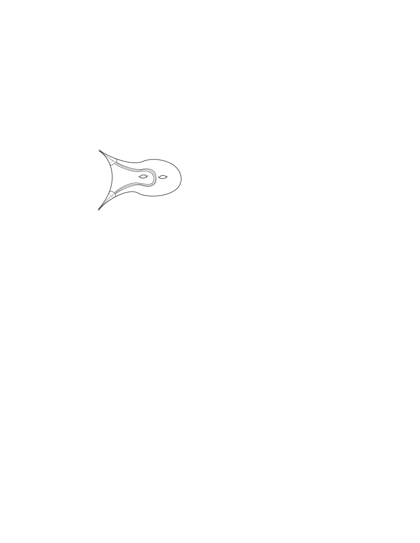
Finally if $\gamma$ has length larger than $L$ outside the $\epsilon$-cusps, let $\gamma_{0}$ denote any arc of $\gamma$ outside the cusps of length $L$, and consider the immersion of $\gamma_{0}\times[-\epsilon,\epsilon]$ taking each $\{p\}\times[-\epsilon,\epsilon]$ to the geodesic segment of length $2\epsilon$ orthogonal to $\gamma$ at its midpoint $p$. The choice of $L_{2}$ and the bound of $2\pi|\chi(S)|$ on the area of $S$ imply that there must be a point $z$ covered with multiplicity 3 by this map. Thus $\gamma$ passes within $\epsilon$ of $z$ three times with (unoriented) directions varying by $O(\epsilon)$ in the projectivized tangent bundle. At least two of those times the orientations match, and we may build $\gamma_{\epsilon}$ as shown in Figure 13. The resulting curve is homotopically nontrivial and non-peripheral because it can be smoothed out to have curvature near 0 and length bounded away from 0. ∎

Figure 13. Constructing $\gamma_{\epsilon}$ when $\gamma$ is long

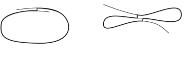
Junctures of convex sets

Lemma 8.6.

Fix $r_{0}>0$. For any $b>0$ there is a $d>0$ such that the following holds: if $A$ and $B$ are convex sets in ${\mathbb{H}}^{3}$, and suppose that $\operatorname{dist}(A,B)\geq r_{0}$. Then

$$\operatorname{diam}({\mathcal{N}}_{b}(A)\cap{\mathcal{N}}_{b}(B))\leq d.$$

Here ${\mathcal{N}}_{b}$ denotes $b$-neighborhood in ${\mathbb{H}}^{3}$.

Proof.

Convexity and the lower bound on $\operatorname{dist}(A,B)$ imply that $A$ and $B$ are contained in disjoint half-spaces $H_{A}$ and $A_{B}$ that are at least $r_{0}$ apart. The intersection ${\mathcal{N}}_{b}(H_{A})\cap{\mathcal{N}}_{b}(H_{B})$ is compact so it has some diameter bound $d$. A sharp value is not hard to compute but we will not need it. ∎

References

- [1] W. Abikoff, The real-analytic theory of Teichmüller space, Springer-Verlag, 1980, Lecture Notes in Mathematics no. 820.
- [2] J. M. Alonso, T. Brady, D. Cooper, V. Ferlini, M. Lustig, M. Mihalik, M. Shapiro, and H. Short, Notes on word hyperbolic groups, Group Theory from a Geometrical Viewpoint, ICTP Trieste 1990 (E. Ghys, A. Haefliger, and A. Verjovsky, eds.), World Scientific, 1991, pp. 3–63.
- [3] L. Bers, Spaces of degenerating Riemann surfaces, Discontinuous groups and Riemann surfaces, Ann. of Math. Stud. 79, Princeton Univ. Press, 1974, pp. 43–59.
- [4] by same author, An inequality for Riemann surfaces, Differential geometry and complex analysis, Springer, Berlin, 1985, pp. 87–93.
- [5] F. Bonahon, Bouts des variétés hyperboliques de dimension 3, Ann. of Math. 124 (1986), 71–158.
- [6] by same author, Geodesic laminations on surfaces, Laminations and Foliations in Dynamics, Geometry and Topology (Stony Brook, NY) (M. Lyubich, J. Milnor, and Y. Minsky, eds.), Contemporary Mathematics, vol. 269, AMS, 2001, pp. 1–37.
- [7] B. Bowditch, Notes on Gromov’s hyperbolicity criterion for path-metric spaces, Group theory from a geometrical viewpoint (Trieste, 1990), World Scientific Publishing, 1991, pp. 64–167.
- [8] J. Brock, Boundaries of Teichmüller spaces and end-invariants for hyperbolic 3-manifolds, Preprint (1999). To appear, Duke Math. J.
- [9] by same author, Iteration of mapping classes and limits of hyperbolic 3-manifolds, Preprint (2000), to appear in Invent. Math.
- [10] by same author, Continuity of Thurston’s length function, Geom. Funct. Anal. 10 (2000), no. 4, 741–797.
- [11] R. Brooks and J. P. Matelski, Collars in Kleinian groups, Duke Math. J. 49 (1982), no. 1, 163–182.
- [12] P. Buser, Geometry and Spectra of Compact Riemann Surfaces, Birkhäuser, 1992.
- [13] R. Canary, M. Culler, S. Hersonsky, and P. Shalen, Density of cusps in boundaries of quasiconformal deformation spaces, in preparation.
- [14] R. D. Canary, On the laplacian and the geometry of hyperbolic 3-manifolds, J. Differential Geom. 36 (1992), 349–367.
- [15] by same author, Algebraic limits of schottky groups, Trans. Amer. Math. Soc. 337 (1993), 235–258.
- [16] R. D. Canary, D. B. A. Epstein, and P. Green, Notes on notes of Thurston, Analytical and Geometric Aspects of Hyperbolic Space, Cambridge University Press, 1987, London Math. Soc. Lecture Notes Series no. 111, pp. 3–92.
- [17] J. Cannon, The theory of negatively curved spaces and groups, Ergodic theory, symbolic dynamics, and hyperbolic spaces (Trieste, 1989), Oxford Univ. Press, 1991, pp. 315–369.
- [18] A. J. Casson and S. A. Bleiler, Automorphisms of surfaces after Nielsen and Thurston, Cambridge University Press, 1988.
- [19] D. B. A. Epstein and A. Marden, Convex hulls in hyperbolic space, a theorem of Sullivan, and measured pleated surfaces, Analytical and Geometric Aspects of Hyperbolic Space, Cambridge University Press, 1987, London Math. Soc. Lecture Notes Series no. 111, pp. 113–254.
- [20] B. Farb and L. Mosher, Schottky subgroups of mapping class groups, In preparation.
- [21] F. Gardiner, Teichmüller theory and quadratic differentials, Wiley Interscience, 1987.
- [22] E. Ghys and P. de la Harpe, Sur les groupes hyperboliques d’aprés Mikhael Gromov, Birkhäuser, 1990.
- [23] M. Gromov, Hyperbolic groups, Essays in Group Theory (S. M. Gersten, editor), MSRI Publications no. 8, Springer-Verlag, 1987.
- [24] J. Harer, Stability of the homology of the mapping class group of an orientable surface, Ann. of Math. 121 (1985), 215–249.
- [25] by same author, The virtual cohomological dimension of the mapping class group of an orientable surface, Invent. Math. 84 (1986), 157–176.
- [26] W. J. Harvey, Boundary structure of the modular group, Riemann Surfaces and Related Topics: Proceedings of the 1978 Stony Brook Conference (I. Kra and B. Maskit, eds.), Ann. of Math. Stud. 97, Princeton, 1981.
- [27] J. Hempel, 3-manifolds as viewed from the curve complex, MSRI Preprint #1997-095 and E-print math.GT/9712220 at http://front.math.ucdavis.edu.
- [28] N. V. Ivanov, Complexes of curves and the Teichmüller modular group, Uspekhi Mat. Nauk 42 (1987), 55–107.
- [29] by same author, The rank of Teichmüller modular groups, Mat. Zametki 44 (1988), no. 5, 636–644, 701, translation in Math. Notes 44 (1988), no. 5-6, 829–832.
- [30] by same author, Complexes of curves and Teichmüller spaces, Math. Notes 49 (1991), 479–484.
- [31] by same author, Subgroups of Teichmüller modular groups, American Mathematical Society, Providence, RI, 1992, translated from the Russian by E. J. F. Primrose and revised by the author.
- [32] by same author, Automorphisms of complexes of curves and of Teichmüller spaces, Internat. Math. Res. Notices (1997), no. 14, 651–666.
- [33] E. Klarreich, The boundary at infinity of the curve complex and the relative Teichmüller space, preprint.
- [34] by same author, Semiconjugacies between Kleinian group actions on the Riemann sphere, Amer. J. Math. 121 (1999), no. 5, 1031–1078.
- [35] J. Lott, -cohomology of geometrically infinite hyperbolic -manifolds, Geom. Funct. Anal. 7 (1997), no. 1, 81–119.
- [36] H. A. Masur and Y. Minsky, Geometry of the complex of curves I: Hyperbolicity, Invent. Math. 138 (1999), 103–149.
- [37] by same author, Geometry of the complex of curves II: Hierarchical structure, Geom. Funct. Anal. 10 (2000), 902–974.
- [38] C. McMullen, Local connectivity, Kleinian groups and geodesics on the blowup of the torus, Preprint: http://www.math.harvard.edu/~ctm/papers.
- [39] by same author, Cusps are dense, Ann. of Math. 133 (1991), 217–247.
- [40] by same author, Renormalization and 3-manifolds which fiber over the circle, Princeton University Press, Princeton, NJ, 1996.
- [41] R. Meyerhoff, A lower bound for the volume of hyperbolic -manifolds., Canad. J. Math. 39 (1987), 1038–1056.
- [42] Y. Minsky, Harmonic maps into hyperbolic 3-manifolds, Trans. Amer. Math. Soc. 332 (1992), 607–632.
- [43] by same author, Teichmüller geodesics and ends of hyperbolic 3-manifolds, Topology 32 (1993), 625–647.
- [44] by same author, On rigidity, limit sets and end invariants of hyperbolic 3-manifolds, J. Amer. Math. Soc. 7 (1994), 539–588.
- [45] by same author, On Thurston’s ending lamination conjecture, Proceedings of Low-Dimensional Topology, May 18-23, 1992, International Press, 1994.
- [46] by same author, The classification of punctured-torus groups, Annals of Math. 149 (1999), 559–626.
- [47] by same author, Kleinian groups and the complex of curves, Geometry and Topology 4 (2000), 117–148.
- [48] by same author, Short geodesics and end invariants, Comprehensive Research on Complex Dynamical Systems and Related Fields (M. Kisaka and S. Morosawa, eds.), vol. 1153, RIMS Kokyuroku, 2000, E-print: arXiv:math.GT/0006002, pp. 1–20.
- [49] K. Ohshika, Ending laminations and boundaries for deformation spaces of Kleinian groups, J. London Math. Soc. 42 (1990), 111–121.
- [50] K. Rafi, Hyperbolic 3-manifolds and geodesics in Teichmüller space, PhD Thesis, SUNY at Stony Brook, 2001.
- [51] W. Thurston, Hyperbolic structures on 3-manifolds, II: surface groups and manifolds which fiber over the circle, E-print: math.GT/9801045 at http://front.math.ucdavis.edu. Original 1986.
- [52] by same author, The geometry and topology of 3-manifolds, Princeton University Lecture Notes, online at http://www.msri.org/publications/books/gt3m, 1982.
- [53] by same author, Three dimensional manifolds, Kleinian groups and hyperbolic geometry, Bull. Amer. Math. Soc. 6 (1982), 357–381.
- [54] by same author, Hyperbolic structures on 3-manifolds, I: deformation of acylindrical manifolds, Ann. of Math. 124 (1986), 203–246.