LOCAL CALIBRATIONS FOR MINIMIZERS OF THE

MUMFORD-SHAH FUNCTIONAL

WITH A TRIPLE JUNCTION

Maria Giovanna Mora

S.I.S.S.A.
via Beirut 2-4, 34014 Trieste, Italy
e-mail: mora@sissa.it

Abstract. We prove that, if $u$ is a function satisfying all Euler conditions for the Mumford-Shah functional and the discontinuity set of $u$ is given by three line segments meeting at the origin with equal angles, then there exists a neighbourhood $U$ of the origin such that $u$ is a minimizer of the Mumford-Shah functional on $U$ with respect to its own boundary conditions on $\partial U$. The proof is obtained by using the calibration method.

Mathematics Subject Classification: 49K10 (49Q20).

Keywords: Mumford-Shah functional, free-discontinuity problems, calibration method.

Ref. S.I.S.S.A. 39/2001/M (May 2001)

a

LOCAL CALIBRATIONS FOR MINIMIZERS OF THE MUMFORD-SHAH

FUNCTIONAL WITH A TRIPLE JUNCTION

Maria Giovanna Mora

Abstract. We prove that, if $u$ is a function satisfying all Euler conditions for the Mumford-Shah functional and the discontinuity set of $u$ is given by three line segments meeting at the origin with equal angles, then there exists a neighbourhood $U$ of the origin such that $u$ is a minimizer of the Mumford-Shah functional on $U$ with respect to its own boundary conditions on $\partial U$. The proof is obtained by using the calibration method.

1 Introduction

The Mumford-Shah functional was proposed in [12] to approach image segmentation problems and it can be written, in the “homogeneous” version in dimension two, as

$$\int_{\Omega}|\nabla u(x,y)|^{2}dx\,dy+{\cal H}^{1}(S_{u}),$$ (1.1)

where $\Omega$ is a bounded open subset of ${\mathbb{R}}^{2}$ with a Lipschitz boundary, ${\cal H}^{1}$ is the one-dimensional Hausdorff measure, $u$ is the unknown function in the space $SBV(\Omega)$ of special functions of bounded variation in $\Omega$, $S_{u}$ is the set of essential discontinuity points of $u$, while $\nabla u$ denotes its approximate gradient (see [4]).

This paper deals with local minimizers of (1.1) with given boundary values. More precisely, we say that $u$ is a Dirichlet minimizer of (1.1) in $\Omega$ if $u$ belongs to $SBV(\Omega)$ and satisfies the inequality

$$\int_{\Omega}|\nabla u(x,y)|^{2}dx\,dy+{\cal H}^{1}(S_{u})\leq\int_{\Omega}|\nabla v(x,y)|^{2}dx\,dy+{\cal H}^{1}(S_{v})$$

for every $v\in SBV(\Omega)$ with the same trace as $u$ on $\partial\Omega$.

Considering different classes of infinitesimal variations, one can show that, if $u$ is a Dirichlet minimizer of (1.1) in $\Omega$, then the following equilibrium conditions (which can be globally called the Euler conditions for (1.1)) are satisfied (see [4] and [12]):

• $u$ is harmonic on $\Omega\setminus S_{u}$;

• the normal derivative of $u$ vanishes on both sides of $S_{u}$, where $S_{u}$ is a regular curve;

• the curvature of $S_{u}$ (where defined) is equal to the difference of the squares of the tangential derivatives of $u$ on both sides of $S_{u}$;

• if $S_{u}$ is locally the union of finitely many regular arcs, then $S_{u}$ can present only two kinds of singularities: either a regular arc ending at some point, the so-called “crack-tip”, or three regular arcs meeting with equal angles of $2\pi/3$, the so-called “triple junction”.

However, since the functional (1.1) is not convex, the Euler conditions are not sufficient for the Dirichlet minimality of $u$.

In [9] it has been proved that, if $S_{u}$ is an analytic curve connecting two points of $\partial\Omega$ (hence, $S_{u}$ has no singular points), then the Euler conditions are also sufficient for the Dirichlet minimality in small domains. In this paper we prove that, if $S_{u}$ is given by three line segments meeting at the origin with equal angles of $2\pi/3$ (i.e., $S_{u}$ is a rectilinear triple junction), the same conclusion holds; in other words, for every $(x,y)\in\Omega$, there is an open neighbourhood $U$ of $(x,y)$ such that $u$ is a Dirichlet minimizer of (1.1) in $U$. Since for $(x,y)\neq(0,0)$ this fact follows from the result in [9], the interesting case is when we restrict the functional to a neighbourhood of the triple point $(0,0)$.

The precise statement of the result is the following.

Theorem 1.1

Let $\Omega:=B(0,1)$ be the open disc in ${\mathbb{R}}^{2}$ with radius $1$ centred at the origin, and let $(A_{0},A_{1},A_{2})$ be the partition of $\Omega$ defined as follows:

$$A_{i}:=\left\{(r\cos\theta,r\sin\theta)\in\Omega:\ 0\leq r<1,\ \frac{2}{3}\pi(2-i)<\theta\leq\frac{2}{3}\pi(3-i)\right\}\qquad\forall\,i=0,1,2.$$

Let $S_{i,j}:=\overline{A_{i}}\cap\overline{A_{j}}$ for every $i<j$. Let $u_{i}\in C^{2}(\overline{A_{i}})$ be a harmonic function in $A_{i}$, satisfying the Neumann conditions on $\partial A_{i}\cap\Omega$ and such that $|\nabla u_{i}|=|\nabla u_{j}|$ on $S_{i,j}$ for every $i<j$. If $u$ is the function in $SBV(\Omega)$ defined by $u:=u_{i}$ a.e. in each $A_{i}$ and $u_{0}(0,0)<u_{1}(0,0)<u_{2}(0,0)$, then there exists a neighbourhood $U$ of the origin such that $u$ is a Dirichlet minimizer in $U$ of the Mumford-Shah functional.

This theorem generalizes the result of Example 4 in [1], where the functions $u_{i}$ were three distinct constants. The proof is obtained by the calibration method adapted in [1] to the functional (1.1). We construct an explicit calibration for $u$ in a cylinder $U{\times}{\mathbb{R}}$, where $U$ is a suitable neighbourhood of $(0,0)$. The symmetry due to the $2\pi/3$-angles is exploited in the whole construction of the calibration; in particular, it allows to deduce from the other Euler conditions that each $u_{i}$ must be either symmetric or antisymmetric with respect to the bisecting line of $A_{i}$ and then, it can be harmonically extended to a neighbourhood of the origin, cut by a half-line in the antisymmetric case. Around the graph of $u$, the calibration is obtained using the gradient field of a family of harmonic functions, whose graphs fibrate a neighbourhood of the graph of $u$; this technique reminds the classical method of the Weierstrass fields, where the minimality of a candidate $u$ is proved by constructing a suitable slope field, starting from a family of solutions of the Euler equation, whose graphs fibrate a neighbourhood of the graph of $u$.

The assumption of $C^{2}$-regularity for $u_{i}$ does not seem too restrictive: indeed, by the regularity results for elliptic problems in non-smooth domains (see [7]), it follows that $u_{i}$ belongs at least to $C^{1}(\overline{A_{i}})$, since $u_{i}$ solves the Laplace equation with Neumann boundary conditions on a sector of angle $2\pi/3$. Moreover, since $u_{i}$ is either symmetric or antisymmetric with respect to the bisecting line of $A_{i}$, one can see $u_{i}$ as a solution of the Laplace equation on a $\pi/3$-sector with Neumann boundary conditions or respectively mixed boundary conditions. By the regularity results in [7], it turns out that in the first case $u_{i}$ belongs to $C^{2}(\overline{A_{i}})$, while in the second one $u_{i}$ can be written as $u_{i}(r,\theta)=\tilde{u}_{i}(r,\theta)+cr^{3/2}\cos\frac{3}{2}\theta$, with $\tilde{u}_{i}\in C^{2}(\overline{A_{i}})$ and $c\in{\mathbb{R}}$. So, only the function $r^{3/2}\cos\frac{3}{2}\theta$ is not recovered by our theorem.

The case where $S_{u}$ is given by three regular curves (not necessarily rectilinear) meeting at a point with $2\pi/3$-angles, is at the moment an open problem and it does not seem to be achievable with a plain arrangement of the calibration used for the rectilinear case, essentially because of the lack of symmetry properties.

The paper is organized as follows. In Section 2 we recall the main result of [1], while Sections 3 – 7 are devoted to the proof of Theorem 1.1: in Section 3 we construct a calibration $\varphi$ in the case $u_{i}$ symmetric and we prove that $\varphi$ satisfies conditions (a), (b), (c), and (e) (see the definition of calibration in Section 2); in Sections 4 and 5 we show some estimates, which will be useful in Section 6 to prove condition (d); finally, in Section 7 we adapt the calibration to the antisymmetric case.

Acknowledgements. The author wish to thank Gianni Dal Maso for many interesting discussions on the subject of this work and for some helpful suggestions about the writing of this paper.

2 Preliminary results

Let $\Omega$ be an open subset of ${\mathbb{R}}^{2}$ with a Lipschitz boundary. If $u$ is a function in $SBV(\Omega)$, for every $(x_{0},y_{0})\in\Omega$ one can define

$$u^{+}(x_{0},y_{0}):=\mathop{\rm ap\,lim\,sup}_{(x,y)\to(x_{0},y_{0})}u(x,y),\qquad u^{-}(x_{0},y_{0}):=\mathop{\rm ap\,lim\,inf}_{(x,y)\to(x_{0},y_{0})}u(x,y).$$

We recall that $S_{u}=\{(x,y)\in\Omega:u^{-}(x,y)<u^{+}(x,y)\}$ and that for ${\cal H}^{1}$-a.e. $(x_{0},y_{0})\in S_{u}$ there exists a (uniquely defined) unit vector $\nu_{u}(x_{0},y_{0})$ (which is normal to $S_{u}$ in an approximate sense) such that

$$\lim_{r\to 0^{+}}\frac{1}{{\cal L}^{2}(B^{\pm}_{r}(x_{0},y_{0}))}\int_{B^{\pm}_{r}(x_{0},y_{0})}|u(x,y)-u^{\pm}(x_{0},y_{0})|\,dx\,dy=0,$$

where $B^{\pm}_{r}(x_{0},y_{0})$ is the intersection of the ball of radius $r$ centred at $(x_{0},y_{0})$ with the half-plane $\{(x,y)\in{\mathbb{R}}^{2}:\pm(x-x_{0},y-y_{0})\cdot\nu_{u}(x_{0},y_{0})\geq 0\}$. For more details see [4].

For every vector field $\varphi:\Omega{\times}{\mathbb{R}}\to{\mathbb{R}}^{2}{\times}{\mathbb{R}}$ we define the maps $\varphi^{xy}:\Omega{\times}{\mathbb{R}}\to{\mathbb{R}}^{2}$ and $\varphi^{z}:\Omega{\times}{\mathbb{R}}\to{\mathbb{R}}$ by

$$\varphi(x,y,z)=(\varphi^{xy}(x,y,z),\varphi^{z}(x,y,z)).$$

We shall consider the collection ${\cal F}$ of all piecewise $C^{1}$ vector fields $\varphi:\Omega{\times}{\mathbb{R}}\to{\mathbb{R}}^{2}{\times}{\mathbb{R}}$ with the following property: there exist a finite family $(U_{i})_{i\in I}$ of pairwise disjoint open subsets of $\Omega{\times}{\mathbb{R}}$ with Lipschitz boundary whose closures cover $\Omega{\times}{\mathbb{R}}$, and a family $(\varphi_{i})_{i\in I}$ of vector fields in $C^{1}(\overline{U_{i}},{\mathbb{R}}^{2}{\times}{\mathbb{R}})$ such that $\varphi$ agrees at any point with one of the $\varphi_{i}$.

Let $u\in SBV(\Omega)$. A calibration for $u$ is a bounded vector field $\varphi\in{\cal F}$ satisfying the following properties:

(a)

${\rm div}\varphi=0$ in the sense of distributions in $\Omega{\times}{\mathbb{R}}$;

(b)

$|\varphi^{xy}(x,y,z)|^{2}\leq 4\varphi^{z}(x,y,z)$ at every continuity point $(x,y,z)$ of $\varphi$;

(c)

$\varphi^{xy}(x,y,u(x,y))=2\nabla u(x,y)$ and $\varphi^{z}(x,y,u(x,y))=|\nabla u(x,y)|^{2}$ for a.e. $(x,y)\in\Omega\setminus S_{u}$;

(d)

$\left|\displaystyle\int_{t_{1}}^{t_{2}}\varphi^{xy}(x,y,z)\,dz\right|^{2}\leq 1$ for every $(x,y)\in\Omega$ and for every $t_{1},t_{2}\in{\mathbb{R}}$;

(e)

$\displaystyle\int_{u^{-}(x,y)}^{u^{+}(x,y)}\varphi^{xy}(x,y,z)\,dz=\nu_{u}(x,y)$ for ${\cal H}^{1}$-a.e. $(x,y)\in S_{u}$.

The following theorem is proved in [1] and [2].

Theorem 2.1

If there exists a calibration $\varphi$ for $u$, then $u$ is a Dirichlet minimizer of the Mumford-Shah functional (1.1) in $\Omega$.

Finally, we present a lemma (proved in [9]), which allows to construct a divergence free vector field starting from a family of harmonic functions.

Lemma 2.2

Let $U$ be an open subset of ${\mathbb{R}}^{2}$ and $I$, $J$ be two real intervals. Let $u:U{\times}J\to I$ be a function of class $C^{1}$ such that

• $u(\cdot,\cdot\,;s)$ is harmonic for every $s\in J$;

• there exists a $C^{1}$ function $t:U{\times}I\to J$ such that $u(x,y\,;t(x,y\,;z))=z$.

If we define in $U{\times}I$ the vector field

$$\phi(x,y,z):=(2\nabla u(x,y\,;t(x,y\,;z)),|\nabla u(x,y\,;t(x,y\,;z))|^{2}),$$

where $\nabla u(x,y\,;t(x,y\,;z))$ denotes the gradient of $u$ with respect to the variables $x,y$ computed at the point $(x,y\,;t(x,y\,;z))$, then $\phi$ is divergence free in $U{\times}I$.

3 Construction of the calibration

Let $\{e^{x},e^{y}\}$ be the canonical basis in ${\mathbb{R}}^{2}$ and for $i=1,2$ consider the vectors $\tau_{i}=(-1/2,(-1)^{i}\sqrt{3}/2)$, $\nu_{i}=((-1)^{i}\sqrt{3}/2,1/2)$, which are tangent and normal to the set $S_{i-1,i}$ (see Fig. 1). As $u_{0}(0,0)<u_{1}(0,0)<u_{2}(0,0)$, there exists an open neighbourhood $U$ of $(0,0)$ such that the function $u$ belongs to $SBV(U)$, the discontinuity set $S_{u}$ of $u$ on $U$ coincides with $\bigcup_{i<j}(S_{i,j}\cap U)$, and the oriented normal vector $\nu_{u}$ to $S_{u}$ is given by

$$\nu_{u}(x,y)=\begin{cases}\nu_{1}&\text{for $(x,y)\in S_{0,1}$,}\\ \nu_{2}&\text{for $(x,y)\in S_{1,2}$,}\\ e^{y}&\text{for $(x,y)\in S_{0,2}$;}\end{cases}$$

by the assumptions on $u_{i}$, the function $u$ satisfies the Euler conditions for (1.1) in $U$. We will construct a local calibration $\varphi=(\varphi^{xy},\varphi^{z}):U{\times}{\mathbb{R}}\to{\mathbb{R}}^{2}{\times}{\mathbb{R}}$ for $u$.

Figure 1: the triple junction.

Applying Schwarz reflection principle with respect to $S_{0,1}$ and $S_{0,2}$, the function $u_{0}$ can be harmonically extended to $U\setminus S_{1,2}$, and analogously $u_{1}$ and $u_{2}$ can be extended to $U\setminus S_{0,2}$ and $U\setminus S_{0,1}$, respectively. By the hypothesis on $u_{i}$ and by Cauchy-Kowalevski Theorem (see [8]) the extension of $u_{0}$ coincides, up to the sign and to additive constants, with $u_{1}$ on $A_{1}$ and with $u_{2}$ on $A_{2}$; analogously, the extension of $u_{1}$ coincides, up to the sign and to an additive constant, with $u_{2}$ on $A_{2}$. Since the composition of the three reflections with respect to $S_{0,1}$, $S_{1,2}$, and $S_{0,2}$ coincides with the reflection with respect to the bisecting line of the sector $A_{0}$, by the previous remarks we can deduce that $u_{0}$ is either symmetric or antisymmetric with respect to the bisecting line of $A_{0}$.

We consider first the case $u_{0}$ symmetric (the antisymmetric case will be studied in Section 7). Then also $u_{1},u_{2}$ are symmetric with respect to the bisecting line of $A_{1},A_{2}$, respectively, and the extensions of $u_{0},u_{1},u_{2}$ by reflection are well defined and harmonic in the whole set $U$.

In order to define the calibration for $u$, let $\varepsilon>0$, $l_{i}\in(u_{i-1}(0,0),u_{i}(0,0))$ for $i=1,2$, and $\lambda>0$ be suitable parameters that will be chosen later, and consider the following subsets of $U{\times}{\mathbb{R}}$:

$$\begin{array}[]{rcll}G_{i}&:=&\{(x,y,z)\in U{\times}{\mathbb{R}}:u_{i}(x,y)-\varepsilon<z<u_{i}(x,y)+\varepsilon\}&\text{for $i=0,1,2$,}\\ K_{i}&:=&\{(x,y,z)\in U{\times}{\mathbb{R}}:l_{i}+\alpha_{i}(x,y)<z<l_{i}+2\lambda+\beta_{i}(x,y)\}&\text{for $i=1,2$,}\\ H_{i}&:=&\{(x,y,z)\in U{\times}{\mathbb{R}}:l_{i}+\lambda/2<z<l_{i}+3\lambda/2\}&\text{for $i=1,2$,}\end{array}$$

where $\alpha_{i}$ and $\beta_{i}$ are suitable Lipschitz functions such that $\alpha_{i}(0,0)=\beta_{i}(0,0)=0$, which will be defined later. If $\varepsilon$ and $\lambda$ are sufficiently small, then for every $i,j$ the sets $G_{i}$, $K_{j}$ are nonempty and disjoint, while for every $i$ the set $H_{i}$ is compactly contained in $K_{i}$, provided $U$ is small enough (see Fig. 2).

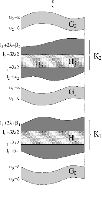
Figure 2: section of the sets $G_{i},K_{i},H_{i}$ at $x=\text{constant}$.

The aim of the definition of the calibration $\varphi$ in $G_{i}$ is to provide a divergence free vector field satisfying condition (c) and such that

$$\begin{array}[]{c}\varphi^{xy}(s\tau_{i},z)\cdot\nu_{i}>0\quad\text{for $u_{i-1}<z<u_{i-1}+\varepsilon$ and for $u_{i}-\varepsilon<z<u_{i}$,}\\ \varphi^{xy}(s\tau_{i},z)\cdot\nu_{i}<0\quad\text{for $u_{i-1}-\varepsilon<z<u_{i-1}$ and for $u_{i}<z<u_{i}+\varepsilon$,}\end{array}$$

for $i=1,2$ and $s\geq 0$, and analogously

$$\begin{array}[]{c}\varphi^{xy}(s,0,z)\cdot e^{y}>0\quad\text{for $u_{0}<z<u_{0}+\varepsilon$ and for $u_{2}-\varepsilon<z<u_{2}$,}\\ \varphi^{xy}(s,0,z)\cdot e^{y}<0\quad\text{for $u_{0}-\varepsilon<z<u_{0}$ and for $u_{2}<z<u_{2}+\varepsilon$;}\end{array}$$

these properties are crucial in order to obtain (d) and (e) simultaneously. Such a field can be obtained by applying the technique shown in Lemma 2.2, starting from the family of harmonic functions $u_{i}+tv_{i}$, where we choose as $v_{i}$ the linear functions defined by

$$v_{0}(x,y):=\tau_{2}\!\cdot\!(x,y)+\varepsilon,\ v_{1}(x,y):=e^{x}\!\cdot\!(x,y)+\varepsilon,\ v_{2}(x,y):=\tau_{1}\!\cdot\!(x,y)+\varepsilon.$$

So for every $(x,y,z)\in G_{i}$, $i=0,1,2$, we define the vector $\varphi(x,y,z)$ as

$$\left(2\nabla u_{i}+2\,\frac{z-u_{i}(x,y)}{v_{i}(x,y)}\nabla v_{i},\left|\nabla u_{i}+\frac{z-u_{i}(x,y)}{v_{i}(x,y)}\nabla v_{i}\right|^{2}\right).$$

The rôle of $K_{i}$ is to give the exact contribution to the integral in (e). In order to annihilate the tangential contribution on $S_{u}$ due to the choice of the field in $G_{i}$, we insert in $K_{i}$ the region $H_{i}$ and for every $(x,y,z)\in H_{i}$, $i=1,2$, we define $\varphi(x,y,z)$ as

$$\left(-\frac{2\varepsilon}{\lambda}\left(\nabla u_{i-1}+\nabla u_{i}\right),\mu\right)$$

where $\mu$ is a positive constant which will be suitably chosen later. By the harmonicity of $u_{i}$ this field is divergence free and, as $\partial_{\nu}u_{i}=0$ on $S_{u}$ for every $i$, its horizontal component is purely tangential on $S_{u}$. So, it remains to correct only the normal contribution to the integral in (e) due to the field in $G_{i}$. To realize this purpose on the two segments $S_{i-1,i}$, $i=1,2$, we could require that $\alpha_{i}(s\tau_{i})=\beta_{i}(s\tau_{i})=0$ for every $s\geq 0$ (see the definition of $K_{i}$) and define $\varphi(x,y,z)$ for $(x,y,z)\in K_{i}\setminus\overline{H_{i}}$ as

$$\left(\frac{1}{\lambda}g\left(\tau_{i}\!\cdot\!(x,y)\right)\nu_{i},\mu\right),$$ (3.1)

where $g$ is a function of real variable chosen in such a way that (e) is satisfied for $(x,y)\in S_{i-1,i}$, i.e.,

$$g(t):=1-\sqrt{3}\frac{\varepsilon^{2}}{v_{0}(t,0)}\qquad\forall t\in{\mathbb{R}},$$

as we will see later in (3.19). Note that the two-dimensional field $g\left(\tau_{i}\!\cdot\!(x,y)\right)\nu_{i}$ is divergence free, since it is with respect to the orthonormal basis $\{\tau_{i},\nu_{i}\}$, hence $\varphi$ is divergence free in $K_{i}\setminus\overline{H_{i}}$; moreover, since $\varphi^{z}\equiv\mu$ on $K_{i}$, the normal component of $\varphi$ is continuous across the boundary of $H_{i}$, so that $\varphi$ turns out to be divergence free in the sense of distributions in the whole set $K_{i}$. Actually it is crucial to add a component along the direction $\tau_{i}$ to the field in (3.1) in order to make (d) true, as it will be clear in the proof of Step 2 (see Section 5); this component has to be chosen in such a way that it is zero on $S_{i-1,i}$ (so that (e) remains valid on these segments) and that it depends only on $\nu_{i}\!\cdot\!(x,y)$ (so that the field remains divergence free). Therefore we replace in (3.1) the vector $g\left(\tau_{i}\!\cdot\!(x,y)\right)\nu_{i}$ by

$$\phi_{i}(x,y):=(-1)^{i+1}f\left(\nu_{i}\!\cdot\!(x,y)\right)\tau_{i}+g\left(\tau_{i}\!\cdot\!(x,y)\right)\nu_{i},$$ (3.2)

where $f$ is an even smooth function of real variable such that $f(0)=0$ and which will be chosen later in a suitable way (see (5.15)). From this definition it follows that

$$\phi_{2}^{x}(x,y)=-\phi_{1}^{x}(x,-y),\qquad\phi_{2}^{y}(x,y)=\phi_{1}^{y}(x,-y),$$ (3.3)

so that

$$\phi_{1}(x,0)+\phi_{2}(x,0)=2\phi_{1}^{y}(x,0)e^{y},$$

i.e., if we assume that $\alpha_{i}(x,0)=\beta_{i}(x,0)$ for every $x\geq 0$, the contribution given by the fields (3.2) to the integral in (e) computed at a point of $S_{0,2}$ is purely normal, as required in (e), but its modulus is in general different from what we need to obtain exactly the normal vector $e^{y}$. In order to correct it, we multiply $\phi_{i}$ by a function $\sigma_{i}$ which is first defined on $S_{i-1,i}\cup S_{0,2}$ (more precisely, $\sigma_{i}$ is taken equal to $1$ on $S_{i-1,i}$ and to the correcting factor on $S_{0,2}$); then, we extend it to a neighbourhood of $(0,0)$ by assuming $\sigma_{i}$ constant along the integral curves of $\phi_{i}$, so that $\sigma_{i}\phi_{i}$ remains divergence free.

The integral curves of $\phi_{i}$ can be represented as the curves $\{(x,y)\in U:y=\psi_{i}(x,s)\}$, where $\psi_{i}(x,s)$ is the solution of the problem

$$\begin{cases}\partial_{x}\psi_{i}(x,s)\phi_{i}^{x}(x,\psi_{i}(x,s))-\phi_{i}^{y}(x,\psi_{i}(x,s))=0,\\ \psi_{i}(s,s)=0,\end{cases}$$ (3.4)

which is defined in a sufficiently small neighbourhood of $(0,0)$. By applying the Implicit Function Theorem, it is easy to see that if $U$ is small enough, then there exists a unique smooth function $h_{i}$ defined in $U$ such that

$$h_{i}(0,0)=0,\qquad\psi_{i}(x,h_{i}(x,y))=y.$$ (3.5)

Note that the curve $\{(x,y)\in U:h_{i}(x,y)=s\}$ coincides with the integral curve $\{(x,y)\in U:y=\psi_{i}(x,s)\}$ and that $(h_{i}(x,y),0)$ gives the intersection point of the integral curve passing through $(x,y)$ with the $x$-axis; in other words, the level lines of $h_{i}$ provide a different representation of the integral curves of $\phi_{i}$ in terms of their intersection point with the $x$-axis.

Figure 3: integral curves of the field $\phi_{1}$.

We state here some properties of $h_{i}$ and $\psi_{i}$ for further references. Since $\psi_{i}(s,s)=0$, we have that

$$h_{i}(s,0)=s$$ (3.6)

for every $s$ such that $(s,0)\in U$. By (3.4) and by differentiating the initial condition in (3.4) with respect to $s$, we obtain

$$\partial_{x}\psi_{i}(0,0)=\frac{\phi_{i}^{y}(0,0)}{\phi_{i}^{x}(0,0)}=\frac{\nu_{i}^{y}}{\nu_{i}^{x}}=\frac{(-1)^{i}}{\sqrt{3}},\qquad\partial_{s}\psi_{i}(0,0)=-\partial_{x}\psi_{i}(0,0)=\frac{(-1)^{i+1}}{\sqrt{3}}.$$ (3.7)

By differentiating the equation in (3.4) with respect to $x$ and to $s$, and by using (3.2), it is easy to see that

$$\partial^{2}_{x}\psi_{i}(0,0)=\partial^{2}_{xs}\psi_{i}(0,0)=0,$$ (3.8)

while by differentiating twice with respect to $s$ the initial condition $\psi_{i}(s,s)=0$, we obtain that

$$\partial^{2}_{s}\psi_{i}(0,0)=-2\partial^{2}_{xs}\psi_{i}(0,0)=0.$$ (3.9)

By (3.7) and (3.8), the curve $\{h_{i}=0\}$ (which coincides with $\{y=\psi_{i}(x,0)\}$) is tangent to $\nu_{i}$ at $0$, which may be an inflection point. Moreover, since $\partial_{x}\psi_{i}(0,0)\neq 0$, by continuity the function $\psi_{i}(\cdot,s)$ is strictly monotone in a small neighbourhood of $0$ for $s$ sufficiently small; by this fact and by comparing the values of the function $\psi_{i}(\cdot,h_{i}(s\tau_{i}))$ at the points $h_{i}(s\tau_{i})$ and $s\tau_{i}^{x}$, it is easy to see that

$$h_{i}(s\tau_{i})\leq 0$$ (3.10)

for every $s\geq 0$ such that $s\tau_{i}\in U$, provided $U$ is small enough. Remark that by (3.6) and (3.10) it follows that the segment $S_{0,2}$ is all contained in the region $\{h_{i}\geq 0\}$, while $S_{i-1,i}$ in the region $\{h_{i}\leq 0\}$.

At last, we set

$$\sigma_{i}(x,y):=\begin{cases}1&\text{if $h_{i}(x,y)\leq 0$,}\\ \displaystyle\frac{g(h_{i}(x,y))}{2\phi_{i}^{y}(h_{i}(x,y),0)}&\text{if $h_{i}(x,y)>0$;}\end{cases}$$

since by definition $\phi_{i}^{y}(0,0)=g(0)\nu_{i}^{y}=g(0)/2$, the function $\sigma_{i}$ is continuous across the curve $\{h_{i}=0\}$. Moreover, remark that from (3.3) it follows that $\psi_{2}(x,s)=-\psi_{1}(x,s)$, $h_{2}(x,y)=h_{1}(x,-y)$, and then

$$\sigma_{2}(x,y)=\sigma_{1}(x,-y).$$ (3.11)

For every $(x,y,z)\in K_{i}\setminus\overline{H_{i}}$, $i=1,2$, we define $\varphi(x,y,z)$ as

$$\left(\frac{1}{\lambda}\sigma_{i}(x,y)\phi_{i}(x,y),\mu\right).$$

In the remaining regions of transition it is convenient to take $\varphi$ purely vertical. In order to make $\varphi$ divergence free in the whole set $U{\times}{\mathbb{R}}$, we need the normal component of $\varphi$ to be continuous across the boundary of $G_{i}$ and $H_{i}$. To guarantee this continuity across $\partial G_{i}$, we are forced to take as third component of $\varphi$ the function

$$\omega(x,y,z):=\begin{cases}\displaystyle\frac{\varepsilon^{2}}{v_{0}^{2}(x,y)}-|\nabla u_{0}|^{2}&\text{for $z<l_{1}+\lambda$,}\\ \\ \displaystyle\frac{\varepsilon^{2}}{v_{1}^{2}(x,y)}-|\nabla u_{1}|^{2}&\text{for $l_{1}+\lambda\leq z<l_{2}+\lambda$,}\\ \\ \displaystyle\frac{\varepsilon^{2}}{v_{2}^{2}(x,y)}-|\nabla u_{2}|^{2}&\text{for $z\geq l_{2}+\lambda$.}\end{cases}$$ (3.12)

Finally, we define the functions $\alpha_{i},\beta_{i}$ in such a way that the normal component of $\varphi$ turns out to be continuous also across the boundary of $K_{i}$; more precisely, for $i=1,2$ we choose $\alpha_{i}$ as the solution of the Cauchy problem

$$\begin{cases}\displaystyle\frac{1}{\lambda}\sigma_{i}(x,y)\phi_{i}(x,y)\cdot\nabla\alpha_{i}(x,y)-\mu=-\frac{\varepsilon^{2}}{v_{i-1}^{2}(x,y)}+|\nabla u_{i-1}(x,y)|^{2},\\ \alpha_{i}(s\tau_{i})=0,\ \alpha_{i}(s,0)=0\quad\text{for $s\geq 0$,}\end{cases}$$

while $\beta_{i}$ as the solution of

$$\begin{cases}\displaystyle\frac{1}{\lambda}\sigma_{i}(x,y)\phi_{i}(x,y)\cdot\nabla\beta_{i}(x,y)-\mu=-\frac{\varepsilon^{2}}{v_{i}^{2}(x,y)}+|\nabla u_{i}(x,y)|^{2},\\ \beta_{i}(s\tau_{i})=0,\ \beta_{i}(s,0)=0\quad\text{for $s\geq 0$.}\end{cases}$$

Since $\sigma_{i}$ is not $C^{1}$ near the curve $\{h_{i}=0\}$, we cannot expect a $C^{1}$ solution. Nevertheless, if $U$ is small enough, then $\alpha_{i},\beta_{i}$ are Lipschitz function defined in $U$, and the possible discontinuity points of $\nabla\alpha_{i},\nabla\beta_{i}$ concentrate only on the curve $\{h_{i}=0\}$; indeed, if $U$ is sufficiently small, the Cauchy problems

$$\begin{cases}\displaystyle\frac{1}{\lambda}\phi_{i}(x,y)\cdot\nabla\tilde{\alpha}_{i}(x,y)-\mu=-\frac{\varepsilon^{2}}{v_{i-1}^{2}(x,y)}+|\nabla u_{i-1}(x,y)|^{2},\\ \tilde{\alpha}_{i}(s\tau_{i})=0\quad(s\in{\mathbb{R}}),\end{cases}$$ (3.13)

and

$$\begin{cases}\displaystyle\frac{g(h_{i}(x,y))}{2\lambda\phi_{i}^{y}(h_{i}(x,y),0)}\phi_{i}(x,y)\cdot\nabla\hat{\alpha}_{i}(x,y)-\mu=-\frac{\varepsilon^{2}}{v_{i-1}^{2}(x,y)}+|\nabla u_{i-1}(x,y)|^{2},\\ \hat{\alpha}_{i}(s,0)=0\quad(s\in{\mathbb{R}}),\end{cases}$$ (3.14)

admit a unique solution $\tilde{\alpha}_{i},\hat{\alpha}_{i}\in C^{\infty}(U)$, since the lines $\{s\tau_{i}:s\in{\mathbb{R}}\}$ and $\{(s,0):s\in{\mathbb{R}}\}$ are not characteristic for these equations. Since the curve $\{h_{i}=0\}$, which coincides with the curve $\{y=\psi_{i}(x,0)\}$, is a characteristic line of both equations (3.13) and (3.14) (use (3.4) and $g(0)/(2\lambda\phi_{i}^{y}(0,0))=1$), the functions $\tilde{\alpha}_{i},\hat{\alpha}_{i}$ assume the same value on the curve $\{h_{i}=0\}$. So, $\alpha_{i}$ can be regarded as the function defined by

$$\alpha_{i}(x,y):=\begin{cases}\tilde{\alpha}_{i}(x,y)&\text{if $h_{i}(x,y)\leq 0$,}\\ \hat{\alpha}_{i}(x,y)&\text{if $h_{i}(x,y)>0$,}\end{cases}$$

and therefore $\alpha_{i}$ is $C^{\infty}$ in $U\setminus\{h_{i}=0\}$, and all derivatives of $\alpha_{i}$ have finite limits on both sides of $\{h_{i}=0\}$. The same argument works for $\beta_{i}$.

The complete definition of the field is therefore the following: for every $(x,y,z)\in U{\times}{\mathbb{R}}$, the vector $\varphi(x,y,z)=(\varphi^{xy},\varphi^{z})(x,y,z)\in{\mathbb{R}}^{2}{\times}{\mathbb{R}}$ is given by

$$\begin{cases}\displaystyle\left(2\nabla u_{i}+2\,\frac{z-u_{i}(x,y)}{v_{i}(x,y)}\nabla v_{i},\left|\nabla u_{i}+\frac{z-u_{i}(x,y)}{v_{i}(x,y)}\nabla v_{i}\right|^{2}\right)&\text{in $G_{i}$ \ $(i=0,1,2)$,}\\ \\ \displaystyle\left(\frac{1}{\lambda}\sigma_{i}(x,y)\phi_{i}(x,y),\mu\right)&\text{in $K_{i}\setminus\overline{H_{i}}$ \ $(i=1,2)$,}\\ \\ \displaystyle\left(-\frac{2\varepsilon}{\lambda}\left(\nabla u_{i-1}+\nabla u_{i}\right),\mu\right)&\text{in $H_{i}$ \ $(i=1,2)$,}\\ \\ \displaystyle\left(0,\omega(x,y,z)\right)&\text{otherwise.}\end{cases}$$

By construction conditions (a) and (c) are satisfied.

Condition (b) is trivial in $G_{i}$ for all $i$.

Since $\nabla u_{i}(0,0)=0$ for all $i$ (this fact easily follows by the assumptions on the regularity of $u_{i}$ and by the Euler conditions), we have that

$$\frac{\varepsilon^{2}}{v^{2}_{i}(0,0)}-|\nabla u_{i}(0,0)|^{2}=1>0;$$

then, if $U$ is small enough,

$$\frac{\varepsilon^{2}}{v^{2}_{i}(x,y)}-|\nabla u_{i}(x,y)|^{2}>0$$

for every $(x,y)\in U$ and for every $i=0,1,2$, and so $\omega$ is always positive.

Arguing in a similar way, if we impose that $\mu>1/(4\lambda^{2})$, condition (b) holds in $K_{i}$, provided $U$ is sufficiently small.

By direct computations we find that for every $(x,y)\in U$

$$\int_{u_{i-1}}^{u_{i}}\varphi^{xy}\ dz =\frac{\varepsilon^{2}}{v_{i-1}}\nabla v_{i-1}-\frac{\varepsilon^{2}}{v_{i}}\nabla v_{i}+\frac{1}{\lambda}(\beta_{i}-\alpha_{i}+\lambda)\sigma_{i}\phi_{i},$$ (3.15)

for $$i=1,2$$, while

$$\int_{u_{0}}^{u_{2}}\varphi^{xy}\ dz =\frac{\varepsilon^{2}}{v_{0}}\nabla v_{0}-\frac{\varepsilon^{2}}{v_{2}}\nabla v_{2}+\frac{1}{\lambda}\sum_{i=1}^{2}(\beta_{i}-\alpha_{i}+\lambda)\sigma_{i}\phi_{i}.$$ (3.16)

Note that for $i=1,2$

$$v_{i-1}(s\tau_{i})=v_{i}(s\tau_{i})=v_{0}(s,0)=\displaystyle-\frac{s}{2}+\varepsilon \forall s\in{\mathbb{R}},$$ (3.17)

$$\nabla v_{i-1}(x,y)-\nabla v_{i}(x,y)=\sqrt{3}\nu_{i} \forall(x,y)\in U.$$ (3.18)

As $h_{i}(s\tau_{i})\leq 0$ for every $s\geq 0$ by (3.10), we have that $\sigma_{i}(s\tau_{i})=1$ for every $s\geq 0$, while by definition $\alpha_{i}(s\tau_{i})=\beta_{i}(s\tau_{i})=0$. From these facts, (3.15), (3.17), (3.18), and the definition of $\phi_{i}$, we obtain

$$\int_{u_{i-1}(s\tau_{i})}^{u_{i}(s\tau_{i})}\varphi^{xy}(s\tau_{i},z)\ dz=\sqrt{3}\frac{\varepsilon^{2}}{v_{0}(s,0)}\nu_{i}+(-1)^{i+1}f(0)\tau_{i}+g(s)\nu_{i}=\nu_{i},$$ (3.19)

where the last equality follows from the definition of $g$ and the fact that $f(0)=0$. Analogously, by the equalities

$$v_{0}(s,0)=v_{2}(s,0) \forall s\in{\mathbb{R}},$$ (3.20)

$$\nabla v_{0}(x,y)-\nabla v_{2}(x,y)=\sqrt{3}e^{y} \forall(x,y)\in U,$$ (3.21)

by the definition of $\alpha_{i}$ and $\beta_{i}$, and by (3.3), (3.11), (3.16), we have

$$\int_{u_{0}(s,0)}^{u_{2}(s,0)}\varphi^{xy}(s,0,z)\ dz = \sqrt{3}\frac{\varepsilon^{2}}{v_{0}(s,0)}e^{y}+2\sigma_{1}(s,0)\phi_{1}^{y}(s,0)e^{y}$$ (3.22)

$$= \sqrt{3}\frac{\varepsilon^{2}}{v_{0}(s,0)}e^{y}+g(s)e^{y}=e^{y},$$

where the two last equalities follow from (3.6) and from the definition of $\sigma_{1}$ and $g$. So condition (e) is satisfied.

The proof of condition (d) will be split in the next three sections: in Section 4 we prove that condition (d) holds if $t_{1}$ and $t_{2}$ belong to suitable neighbourhoods of $u_{i-1}(0,0)$ and $u_{i}(0,0)$, respectively; then, in Section 5 we prove condition (d) for $t_{1}$ and $t_{2}$ belonging to suitable neighbourhoods of $u_{0}(0,0)$ and $u_{2}(0,0)$, respectively; finally, in Section 6, by a continuity argument we show that condition (d) is true in all other cases.

4 Estimates for $t_{1}$ and $t_{2}$ near $u_{i-1}$ and $u_{i}$

For $(x,y)\in U$ and $t_{1},t_{2}\in{\mathbb{R}}$, we set

$$I(x,y,t_{1},t_{2}):=\int_{t_{1}}^{t_{2}}\varphi^{xy}(x,y,z)\,dz$$ (4.1)

and we denote its absolute value by $\rho$. In this section, we will show that $\rho(x,y,t_{1},t_{2})\leq 1$ in a neighbourhood of the point $(0,0,u_{i-1}(0,0),u_{i}(0,0))$ for $i=1,2$, so that the following step will be proved.

Step 1.– For a suitable choice of the parameter $\varepsilon$, there exists $\delta>0$ such that condition (d) holds for $|t_{1}-u_{i-1}(0,0)|<\delta$, $|t_{2}-u_{i}(0,0)|<\delta$ with $i=1,2$, provided $U$ is small enough.

Note that $\rho$ is a continuous function, but its derivatives with respect to $x,y$ may be discontinuous at the points $(x,y,t_{1},t_{2})$ such that $h_{1}(x,y)=0$ or $h_{2}(x,y)=0$; indeed, the curve $\{h_{i}=0\}$ is the boundary of the different regions of definition of the functions $\sigma_{i}$, $\alpha_{i}$, and $\beta_{i}$, whose derivatives may present therefore some discontinuities. Nevertheless, if we set $N_{i}:=\{(x,y)\in U:h_{i}(x,y)<0\}$ and $P_{i}:=\{(x,y)\in U:h_{i}(x,y)>0\}$, the restrictions of $\sigma_{i}$, $\alpha_{i}$, and $\beta_{i}$ to the sets $N_{i}$ and $P_{i}$ can be extended up to the boundary $\{h_{i}=0\}$ as $C^{\infty}$ functions; so, along the curve $\{h_{i}=0\}$ the traces of the derivatives of $\sigma_{i}$, $\alpha_{i}$, and $\beta_{i}$ are defined. Then, also the traces of the derivatives of $\rho$ with respect to $x,y$ are defined at the points $(x,y,t_{1},t_{2})$ with $h_{1}(x,y)=0$ or $h_{2}(x,y)=0$.

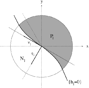
Figure 4: the regions $P_{1}$ and $N_{1}$.

Since we want to study the behaviour of $\rho$ in a neighbourhood of $(0,0,u_{i-1}(0,0),u_{i}(0,0))$, we can suppose $|t_{1}-u_{i-1}(0,0)|\leq\varepsilon$ and $|t_{2}-u_{i}(0,0)|\leq\varepsilon$, so that the possible discontinuities of the derivatives of $\rho$ concentrate only on the curve $\{h_{i}=0\}$. We study separately the two regions $N_{i}$ and $P_{i}$.

Consider first the case $(x,y)\in\overline{N_{i}}$, which is the region containing $S_{i-1,i}$. We will study the derivatives of $\rho$ at the points of the form

$$q_{i}(s):=(s\tau_{i},u_{i-1}(s\tau_{i}),u_{i}(s\tau_{i})),\qquad s\geq 0.$$

We have already shown (condition (e)) that $\rho(q_{i}(s))=1$ for every $s\geq 0$; we want to prove that

$$\nabla\rho(q_{i}(s))=0\qquad\forall s\geq 0$$ (4.2)

(where now $\nabla$ denotes the gradient with respect to $x,y,t_{1},t_{2}$) and that the Hessian matrix of $\rho$ with respect to $\nu_{i},t_{1},t_{2}$ is negative definite at $q_{i}(0)$.

Let $I^{\tau_{i}}$ and $I^{\nu_{i}}$ be the components of the integral in (4.1) along the directions $\tau_{i}$ and $\nu_{i}$, respectively. Since by definition

$$\rho(x,y,t_{1},t_{2})=[(I^{\tau_{i}}(x,y,t_{1},t_{2}))^{2}+(I^{\nu_{i}}(x,y,t_{1},t_{2}))^{2}]^{1/2},$$

the gradient of $\rho$ is given by

$$\nabla\rho=\frac{1}{\rho}(I^{\tau_{i}}\nabla I^{\tau_{i}}+I^{\nu_{i}}\nabla I^{\nu_{i}}).$$ (4.3)

Note that (3.19) implies that

$$I^{\tau_{i}}(q_{i}(s))=0\qquad\text{and}\qquad I^{\nu_{i}}(q_{i}(s))=1\qquad\forall s\geq 0,$$ (4.4)

hence

$$\nabla\rho(q_{i}(s))=\nabla I^{\nu_{i}}(q_{i}(s)).$$ (4.5)

By the definition of $\varphi$ in $G_{i}$ and by (3.15) we can compute explicitly the expression of $I^{\nu_{i}}$ at $(x,y,t_{1},t_{2})$:

$$I^{\nu_{i}}=-2(t_{1}-u_{i-1})\partial_{\nu_{i}}u_{i-1}+2(t_{2}-u_{i})\partial_{\nu_{i}}u_{i}+\frac{1}{\lambda}(\beta_{i}-\alpha_{i}+\lambda)\sigma_{i}\phi_{i}^{\nu_{i}}\\ +\frac{\sqrt{3}}{2v_{i-1}}(\varepsilon^{2}-(t_{1}-u_{i-1})^{2})+\frac{\sqrt{3}}{2v_{i}}(\varepsilon^{2}-(t_{2}-u_{i})^{2}),$$ (4.6)

where

$$\phi_{i}^{\tau_{i}}(x,y)=(-1)^{i+1}f(\nu_{i}\!\cdot\!(x,y))\qquad\text{and}\qquad\phi_{i}^{\nu_{i}}(x,y)=g(\tau_{i}\!\cdot\!(x,y)).$$ (4.7)

By differentiating (4.6) with respect to the direction $\nu_{i}$ we obtain

$$\partial_{\nu_{i}}I^{\nu_{i}}=2(\partial_{\nu_{i}}u_{i-1})^{2}-2(\partial_{\nu_{i}}u_{i})^{2}-2(t_{1}-u_{i-1})\partial^{2}_{\nu_{i}}u_{i-1}+2(t_{2}-u_{i})\partial^{2}_{\nu_{i}}u_{i}\\ +\frac{1}{\lambda}\partial_{\nu_{i}}(\beta_{i}-\alpha_{i})\sigma_{i}\phi_{i}^{\nu_{i}}+\frac{1}{\lambda}(\beta_{i}-\alpha_{i}+\lambda)(\partial_{\nu_{i}}\sigma_{i}\phi_{i}^{\nu_{i}}+\sigma_{i}\partial_{\nu_{i}}\phi_{i}^{\nu_{i}})\\ -\frac{3}{4v_{i-1}^{2}}(\varepsilon^{2}-(t_{1}-u_{i-1})^{2})+\frac{3}{4v_{i}^{2}}(\varepsilon^{2}-(t_{2}-u_{i})^{2})\\ +\frac{\sqrt{3}}{v_{i-1}}(t_{1}-u_{i-1})\partial_{\nu_{i}}u_{i-1}+\frac{\sqrt{3}}{v_{i}}(t_{2}-u_{i})\partial_{\nu_{i}}u_{i}.$$ (4.8)

By the Euler conditions, $\partial_{\nu_{i}}u_{i-1}(s\tau_{i})=\partial_{\nu_{i}}u_{i}(s\tau_{i})=0$ for every $s\geq 0$. Moreover, since $|\nabla u_{i-1}|=|\nabla u_{i}|$ on $U$ (see the remark at the beginning of the proof), in the region $\overline{N_{i}}$ the function $\beta_{i}-\alpha_{i}$ coincides with the solution $\xi_{i}$ of the problem

$$\begin{cases}\displaystyle\frac{1}{\lambda}\phi_{i}^{\tau_{i}}\partial_{\tau_{i}}\xi_{i}+\frac{1}{\lambda}\phi_{i}^{\nu_{i}}\partial_{\nu_{i}}\xi_{i}=\frac{\varepsilon^{2}}{v_{i-1}^{2}}-\frac{\varepsilon^{2}}{v_{i}^{2}},\\ \xi_{i}(s\tau_{i})=0\quad(s\geq 0).\end{cases}$$ (4.9)

As $\partial_{\tau_{i}}\xi_{i}(s\tau_{i})=0$ and $v_{i-1}(s\tau_{i})=v_{i}(s\tau_{i})$ for every $s\geq 0$ (see (3.17)), we have that

$$\partial_{\nu_{i}}(\beta_{i}-\alpha_{i})(s\tau_{i})=\partial_{\nu_{i}}\xi_{i}(s\tau_{i})=0.$$ (4.10)

By definition $\partial_{\nu_{i}}\phi_{i}^{\nu_{i}}\equiv 0$ and $\sigma_{i}(x,y)=1$ for every $(x,y)\in\overline{N_{i}}$; using these remarks and the first equality in (3.17), we can deduce that

$$\partial_{\nu_{i}}I^{\nu_{i}}(q_{i}(s))=0$$ (4.11)

for every $s>0$, and the equality holds also for the trace of $\partial_{\nu_{i}}I^{\nu_{i}}$ at $q_{i}(0)$. Since the derivatives of $I^{\nu_{i}}$ with respect to $t_{1}$ and $t_{2}$ are given by

$$\partial_{t_{1}}I^{\nu_{i}}=-2\partial_{\nu_{i}}u_{i-1}-\frac{\sqrt{3}}{v_{i-1}}(t_{1}-u_{i-1}),\qquad\partial_{t_{2}}I^{\nu_{i}}=2\partial_{\nu_{i}}u_{i}-\frac{\sqrt{3}}{v_{i}}(t_{2}-u_{1}),$$ (4.12)

by the Euler conditions it follows that

$$\partial_{t_{1}}I^{\nu_{i}}(q_{i}(s))=\partial_{t_{2}}I^{\nu_{i}}(q_{i}(s))=0.$$ (4.13)

As $I^{\nu_{i}}(q_{i}(s))=1$ for every $s\geq 0$, equalities (4.13) imply that $\partial_{\tau_{i}}I^{\nu_{i}}(q_{i}(s))=0$. By this fact, (4.5), (4.11), and (4.13), equality (4.2) is proved.

Now we need to compute the trace of the Hessian matrix of $\rho$ with respect to $\nu_{i},t_{1},t_{2}$ at the point $q_{i}(0)$; using (4.4) (4.11), (4.13) and (4.2), the Hessian matrix at $q_{i}(0)$ reduces to

$$\nabla^{2}_{\nu_{i}t_{1}t_{2}}\rho(q_{i}(0))=[\nabla_{\!\nu_{i}t_{1}t_{2}}I^{\tau_{i}}\otimes\nabla_{\!\nu_{i}t_{1}t_{2}}I^{\tau_{i}}+\nabla^{2}_{\nu_{i}t_{1}t_{2}}I^{\nu_{i}}](q_{i}(0)),$$ (4.14)

where $\nabla_{\!\nu_{i}t_{1}t_{2}}$ denotes the gradient with respect to $\nu_{i},t_{1},t_{2}$ and $\otimes$ the tensor product. As before, we know the explicit expression of $I^{\tau_{i}}$:

$$I^{\tau_{i}}=-2(t_{1}-u_{i-1})\partial_{\tau_{i}}u_{i-1}+2(t_{2}-u_{i})\partial_{\tau_{i}}u_{i}+\frac{1}{\lambda}(\beta_{i}-\alpha_{i}+\lambda)\sigma_{i}\phi_{i}^{\tau_{i}}\\ -\frac{1}{2v_{i-1}}(\varepsilon^{2}-(t_{1}-u_{i-1})^{2})+\frac{1}{2v_{i}}(\varepsilon^{2}-(t_{2}-u_{i})^{2}),$$ (4.15)

hence, using the Euler conditions, (4.10), and the fact that $\sigma_{i}\equiv 1$ in $\overline{N_{i}}$, it results that

$$\partial_{\nu_{i}}I^{\tau_{i}}(q_{i}(0))=\frac{1}{2}\partial_{\nu_{i}}v_{i-1}(0,0)-\frac{1}{2}\partial_{\nu_{i}}v_{i}(0,0)+\partial_{\nu_{i}}\phi_{i}^{\tau_{i}}(0,0)=\frac{\sqrt{3}}{2},$$ (4.16)

where the last equality follows by (3.18) and by the equality

$$\partial_{\nu_{i}}\phi_{i}^{\tau_{i}}(0)=(-1)^{i+1}f^{\prime}(0)=0.$$ (4.17)

By differentiating (4.8) and by using the Euler conditions, (4.10), the constancy of $\sigma_{i}$ in $\overline{N_{i}}$, and the fact that $\partial^{2}_{\nu_{i}}\phi_{i}^{\nu_{i}}\equiv 0$, we have

$$\partial^{2}_{\nu_{i}}I^{\nu_{i}}(q_{i}(0))=\frac{1}{\lambda}\phi_{i}^{\nu_{i}}(0,0)\partial^{2}_{\nu_{i}}(\beta_{i}-\alpha_{i})(0,0)+\frac{3}{2\varepsilon}\partial_{\nu_{i}}v_{i-1}(0,0)-\frac{3}{2\varepsilon}\partial_{\nu_{i}}v_{i}(0,0)=-\frac{\sqrt{3}}{2\varepsilon},$$ (4.18)

where the last equality follows from

$$\frac{1}{\lambda}\phi_{i}^{\nu_{i}}(0,0)\partial^{2}_{\nu_{i}}(\beta_{i}-\alpha_{i})(0,0)=-\frac{2\sqrt{3}}{\varepsilon},$$ (4.19)

which can be obtained by differentiating (4.9). Using (4.14), (4.16), and (4.18), we obtain that

$$\partial^{2}_{\nu_{i}}\rho(q_{i}(0))=[\partial_{\nu_{i}}I^{\tau_{i}}(q_{i}(0))]^{2}+\partial^{2}_{\nu_{i}}I^{\nu_{i}}(q_{i}(0))=\frac{3}{4}-\frac{\sqrt{3}}{2\varepsilon}<0,$$ (4.20)

provided $\varepsilon$ is sufficiently small. Since $\partial_{t_{1}}I^{\tau_{i}}(q_{i}(0))=0$ (this can be easily proved using the fact that $\nabla u_{i-1}(0,0)=\nabla u_{i}(0,0)=0$), by (4.14) we have that

$$\partial^{2}_{\nu_{i}t_{1}}\rho(q_{i}(0))=\partial^{2}_{\nu_{i}t_{1}}I^{\nu_{i}}(q_{i}(0)),\qquad\partial^{2}_{t_{1}}\rho(q_{i}(0))=\partial^{2}_{t_{1}}I^{\nu_{i}}(q_{i}(0)).$$

By differentiating (4.12) and by using the Euler conditions, it turns out that

$$\partial^{2}_{\nu_{i}t_{1}}I^{\nu_{i}}(q_{i}(0))=-2\partial^{2}_{\nu_{i}}u_{i-1}(0,0),\qquad\partial^{2}_{t_{1}}I^{\nu_{i}}(q_{i}(0))=-\frac{\sqrt{3}}{\varepsilon},$$

so that

$$\det\left(\begin{array}[]{cc}\partial^{2}_{\nu_{i}}\rho&\partial^{2}_{\nu_{i}t_{1}}\rho\vspace{.1cm}\\ \partial^{2}_{\nu_{i}t_{1}}\rho&\partial^{2}_{t_{1}}\rho\end{array}\right)(q_{i}(0))=\frac{3}{2\varepsilon^{2}}\left(1-\frac{\sqrt{3}}{2}\varepsilon\right)-4(\partial^{2}_{\nu_{i}}u_{i-1}(0,0))^{2}.$$

Arguing in a similar way, one can find that

$$\partial^{2}_{\nu_{i}t_{2}}\rho(q_{i}(0))=2\partial^{2}_{\nu_{i}}u_{i}(0,0),\quad\partial^{2}_{t_{2}}\rho(q_{i}(0))=-\frac{\sqrt{3}}{\varepsilon},\quad\partial^{2}_{t_{1}t_{2}}\rho(q_{i}(0))=0,$$

so that

$$\det\nabla^{2}_{\nu_{i}t_{1}t_{2}}\rho(q_{i}(0))=-\frac{3\sqrt{3}}{2\varepsilon^{3}}\left(1-\frac{\sqrt{3}}{2}\varepsilon\right)+\frac{4\sqrt{3}}{\varepsilon}[(\partial^{2}_{\nu_{i}}u_{i-1}(0,0))^{2}+(\partial^{2}_{\nu_{i}}u_{i}(0,0))^{2}].$$

Since for $\varepsilon$ sufficiently small it results that

$$\det\left(\begin{array}[]{cc}\partial^{2}_{\nu_{i}}\rho&\partial^{2}_{\nu_{i}t_{1}}\rho\vspace{.1cm}\\ \partial^{2}_{\nu_{i}t_{1}}\rho&\partial^{2}_{t_{1}}\rho\end{array}\right)(q_{i}(0))>0,\qquad\det\nabla^{2}_{\nu_{i}t_{1}t_{2}}\rho(q_{i}(0))<0,$$ (4.21)

then, by (4.20) and (4.21) the Hessian matrix of $\rho$ at $q_{i}(0)$ is negative definite.

At this point we have all the ingredients we need in order to compare the value of $\rho$ on $S_{i-1,i}$ with its value at a point $(x,y,t_{1},t_{2})$ for $(x,y)\in\overline{N_{i}}$ and $|t_{1}-u_{i-1}(0,0)|\leq\varepsilon$, $|t_{2}-u_{i}(0,0)|\leq\varepsilon$.

Remark that since the curve $\{h_{i}=0\}$ may have an inflection point at the origin, the set $\overline{N_{i}}$ might be not convex. If the segment joining $(x,y)$ with its orthogonal projection on $S_{i-1,i}$ (which is a point of the form $s\tau_{i}$ with $s\geq 0$) is all contained in $\overline{N_{i}}$, then we can consider the restriction of $\rho$ to the segment joining $(x,y,t_{1},t_{2})$ with $q_{i}(s)$ and write its Taylor expansion of second order centred at $q_{i}(s)$. By (4.2) and the fact that the Hessian matrix of $\rho$ is negative definite at $q_{i}(0)$ (and then, by continuity in a small neighbourhood), we have that there exist $\delta,C>0$ such that, if $U$ is small enough and $|t_{1}-u_{i-1}(0,0)|<\delta$, $|t_{2}-u_{i}(0,0)|<\delta$, then

$$\rho(x,y,t_{1},t_{2})\leq 1-C(\nu_{i}\!\cdot\!(x,y))^{2}-C(t_{1}-u_{i-1}(s\tau_{i}))^{2}-C(t_{2}-u_{i}(s\tau_{i}))^{2}\leq 1.$$

In the general case, since the curve $\{y=\psi_{i}(x,0)\}$ is $C^{2}$ with null second derivative at $0$, one can find $s>0$, $a\in{\mathbb{R}}$ such that the segment joining $(x,y)$ with $s\tau_{i}+a\nu_{i}$ is all contained in ${\overline{N}_{i}}$ and the ratio $|(x,y)-s\tau_{i}-a\nu_{i}|/a^{2}$ is infinitesimal as $a\to 0$. Since $s>0$, the segment joining $s\tau_{i}+a\nu_{i}$ with its projection $s\tau_{i}$ on $S_{i-1,i}$ is all contained in ${\overline{N}_{i}}$, so that we can apply to this point the estimate above; if we call $L$ the $L^{\infty}$-norm of the gradient of $\rho$, we obtain that

$$\rho(x,y,t_{1},t_{2}) \leq \rho(s\tau_{i}+a\nu_{i},t_{1},t_{2})+L|(x,y)-s\tau_{i}-a\nu_{i}|$$

$$\leq 1-a^{2}\left(C-L\frac{|(x,y)-s\tau_{i}-a\nu_{i}|}{a^{2}}\right)-C(t_{1}-u_{i-1}(s\tau_{i}))^{2}-C(t_{2}-u_{i}(s\tau_{i}))^{2},$$

which is less than $1$, provided $U$ is small enough. So we have proved that, if $\varepsilon$ is sufficiently small, then there exists $\delta>0$ such that

$$\rho(x,y,t_{1},t_{2})\leq 1\qquad\text{for}\ (x,y)\in\overline{N_{i}},\ |t_{1}-u_{i-1}(0,0)|<\delta,\ |t_{2}-u_{i}(0,0)|<\delta,$$ (4.22)

provided $U$ is sufficiently small.

Suppose now $(x,y)\in\overline{P_{i}}$, $|t_{1}-u_{i-1}(0,0)|\leq\varepsilon$, $|t_{2}-u_{i}(0,0)|\leq\varepsilon$. In order to show that $\rho\leq 1$ also in this case, we will compute the traces of the gradient and of the Hessian matrix of $\rho$ at the point $q_{i}(0)$. The main difference with respect to the previous case is that in the region $\overline{P_{i}}$ the function $\beta_{i}-\alpha_{i}$ coincides with the solution $\eta_{i}$ of the problem

$$\begin{cases}\displaystyle\frac{1}{\lambda}\sigma_{i}(x,y)\phi_{i}(x,y)\cdot\nabla\eta_{i}(x,y)=\frac{\varepsilon^{2}}{v_{i-1}^{2}(x,y)}-\frac{\varepsilon^{2}}{v_{i}^{2}(x,y)},\\ \eta_{i}(s,0)=0\quad(s\geq 0),\end{cases}$$ (4.23)

while the function $\sigma_{i}$ is defined as

$$\sigma_{i}(x,y)=\frac{g(h_{i}(x,y))}{2\phi_{i}^{y}(h_{i}(x,y),0)}\qquad\forall(x,y)\in\overline{P_{i}}.$$ (4.24)

By (4.4) and (4.3) it follows that

$$\nabla\rho(q_{i}(0))=\nabla I^{\nu_{i}}(q_{i}(0)).$$ (4.25)

By (4.6) we obtain the following expression for the gradient of $I^{\nu_{i}}$ with respect to $\tau_{i},\nu_{i}$ computed at the point $q_{i}(0)$:

$$\nabla_{\!\tau_{i}\nu_{i}}I^{\nu_{i}}(q_{i}(0))=g(0)\nabla\sigma_{i}(0,0)+\nabla\phi_{i}^{\nu_{i}}(0,0)+\frac{\sqrt{3}}{2}\tau_{i},$$ (4.26)

where we have used the Euler conditions, the fact that $\nabla(\beta_{i}-\alpha_{i})(0,0)=0$ by (4.23), and that

$$\nabla v_{i-1}(x,y)+\nabla v_{i}(x,y)=-\tau_{i}\qquad\forall(x,y)\in U.$$

It follows immediately by (4.7) that

$$\nabla\phi_{i}^{\nu_{i}}(x,y)=g^{\prime}(\tau_{i}\!\cdot\!(x,y))\tau_{i}$$ (4.27)

and by the definition of $g$ that

$$g^{\prime}(t)=\sqrt{3}\varepsilon^{2}\frac{\partial_{x}v_{0}(t,0)}{v^{2}_{0}(t,0)}=-\frac{\sqrt{3}}{2}\varepsilon^{2}\frac{1}{v^{2}_{0}(t,0)}$$ (4.28)

for all $t\in{\mathbb{R}}$. By differentiating (4.24), we obtain that

$$\nabla\sigma_{i}(x,y)=\frac{1}{2}p(h_{i}(x,y))\nabla h_{i}(x,y),$$ (4.29)

where we have set

$$p(t):=\frac{g^{\prime}(t)}{\phi_{i}^{y}(t,0)}-\frac{g(t)}{[\phi_{i}^{y}(t,0)]^{2}}\partial_{x}\phi_{i}^{y}(t,0).$$

To compute the gradient of $h_{i}$ it is enough to differentiate the second equality in (3.5): this provides

$$\partial_{x}\psi_{i}(x,h_{i})+\partial_{s}\psi_{i}(x,h_{i})\partial_{x}h_{i}=0,\qquad\partial_{s}\psi_{i}(x,h_{i})\partial_{y}h_{i}=1;$$ (4.30)

by (3.7) we have that

$$\nabla h_{i}(0,0)=-2\tau_{i}.$$ (4.31)

Since

$$\partial_{x}\phi_{i}^{y}(x,y)=(-1)^{i+1}\frac{3}{4}f^{\prime}(\nu_{i}\!\cdot\!(x,y))-\frac{1}{4}g^{\prime}(\tau_{i}\!\cdot\!(x,y)),$$

we find that $p(0)=3g^{\prime}(0)/g(0)$, and substituting in (4.29), we have that

$$\nabla\sigma_{i}(0,0)=-3\frac{g^{\prime}(0)}{g(0)}\tau_{i}.$$ (4.32)

Since the partial derivatives of $I^{\nu_{i}}$ with respect to $t_{1}$ and $t_{2}$ are still given by (4.12), they are equal to $0$ at the point $q_{i}(0)$, as in the previous case. Then, by (4.25), (4.26), (4.27), (4.32), and (4.28), we deduce that

$$\nabla\rho(q_{i}(0))=\left(\frac{3\sqrt{3}}{2}\tau_{i},0,0\right).$$ (4.33)

To conclude the study of $\rho$ in this region, we write the Hessian matrix of $\rho$ with respect to $\nu_{i},t_{1},t_{2}$, which still satisfies (4.14). Differentiating (4.15) and using the Euler conditions, the fact that $\nabla(\beta_{i}-\alpha_{i})(0,0)=0$, $\phi_{i}^{\tau_{i}}(0,0)=0$ and (4.17), we obtain that (4.16) still holds. Differentiating (4.8) and computing the result at $q_{i}(0)$, we have that

$$\partial^{2}_{\nu_{i}}I^{\nu_{i}}(q_{i}(0))=\frac{1}{\lambda}g(0)\partial^{2}_{\nu_{i}}(\beta_{i}-\alpha_{i})(0,0)+g(0)\partial^{2}_{\nu_{i}}\sigma_{i}(0,0)+\frac{3}{2\varepsilon}(\partial_{\nu_{i}}v_{i-1}(0,0)-\partial_{\nu_{i}}v_{i}(0,0)),$$ (4.34)

where we have used in particular that $\partial_{\nu_{i}}\sigma_{i}(0,0)=0$ by (4.32) and that $\partial^{2}_{\nu_{i}}\phi_{i}^{\nu_{i}}\equiv 0$. In order to compute the second derivative of $\beta_{i}-\alpha_{i}$ with respect to the direction $\nu_{i}$, we differentiate (4.23) with respect to $x$ and with respect to $y$; using the fact that $\partial_{x}(\beta_{i}-\alpha_{i})(s,0)=0$ for every $s\geq 0$, we obtain

$$\partial^{2}_{x}(\beta_{i}-\alpha_{i})(0,0)=0,\qquad\partial^{2}_{xy}(\beta_{i}-\alpha_{i})(0,0)=\displaystyle\frac{6}{\varepsilon}(-1)^{i+1}\frac{\lambda}{g(0)},$$ (4.35)

$$\partial^{2}_{y}(\beta_{i}-\alpha_{i})(0,0)=\displaystyle-\frac{2\sqrt{3}}{\varepsilon}\frac{\lambda}{g(0)}+\sqrt{3}(-1)^{i+1}\partial^{2}_{xy}(\beta_{i}-\alpha_{i})(0,0)=\frac{4\sqrt{3}}{\varepsilon}\frac{\lambda}{g(0)}.$$ (4.36)

By the relation $\partial^{2}_{\nu_{i}}=\frac{3}{4}\partial^{2}_{x}+\frac{\sqrt{3}}{2}(-1)^{i}\partial^{2}_{xy}+\frac{1}{4}\partial^{2}_{y}$, it follows that

$$\partial^{2}_{\nu_{i}}(\beta_{i}-\alpha_{i})(0,0)=-\frac{2\sqrt{3}}{\varepsilon}\frac{\lambda}{g(0)}.$$

Since $\partial_{\nu_{i}}h_{i}(0,0)=0$ by (4.31), from (4.29) we obtain that

$$\partial^{2}_{\nu_{i}}\sigma_{i}(0,0)=\frac{1}{2}\left(\frac{g^{\prime}(0)}{\phi_{i}^{y}(0,0)}-\frac{g(0)}{[\phi_{i}^{y}(0,0)]^{2}}\partial_{x}\phi_{i}^{y}(0,0)\right)\partial^{2}_{\nu_{i}}h_{i}(0,0)=\frac{3}{2}\frac{g^{\prime}(0)}{g(0)}\partial^{2}_{\nu_{i}}h_{i}(0).$$ (4.37)

By differentiating twice with respect to the direction $\nu_{i}$ the second equality in (3.5), we obtain that

$$(\nu_{i}^{x})^{2}\partial^{2}_{x}\psi_{i}(x,h_{i})+2\nu_{i}^{x}\partial^{2}_{xs}\psi_{i}(x,h_{i})\partial_{\nu_{i}}h_{i}+\partial^{2}_{s}\psi_{i}(x,h_{i})(\partial_{\nu_{i}}h_{i})^{2}+\partial_{s}\psi_{i}(x,h_{i})\partial^{2}_{\nu_{i}}h_{i}=0;$$

since $\partial_{\nu_{i}}h_{i}(0,0)=0$ by (4.31) and $\partial^{2}_{x}\psi_{i}(0,0)=0$ by (3.8), we can conclude that $\partial^{2}_{\nu_{i}}h_{i}(0,0)=0$ and then, by (4.37) also the limit of $\partial^{2}_{\nu_{i}}\sigma_{i}$ at $(0,0)$ is equal to $0$. Taking (3.17) and (4.34) into account, we can conclude that

$$\partial^{2}_{\nu_{i}}I^{\nu_{i}}(q_{i}(0))=-\frac{\sqrt{3}}{2\varepsilon},$$

i.e., (4.18) is still satisfied. Since it is easy to see that also the other second derivatives of $\rho$ remain unchanged, we can conclude that the Hessian matrix of $\rho$ with respect to $\nu_{i},t_{1},t_{2}$ is negative definite at $q_{i}(0)$.

If the segment joining $(x,y,t_{1},t_{2})$ with $q_{i}(0)$ is all contained in $\overline{P_{i}}$, then we consider the Taylor expansion of second order centred at $q_{i}(0)$ of the function $\rho$ restricted to this segment; since the component of $(x,y)$ along $\tau_{i}$ is less or equal than $0$, by (4.33) and by the fact that the Hessian matrix of $\rho$ with respect to $\nu_{i},t_{1},t_{2}$ is negative definite, we have that there exists $\delta>0$ such that $\rho(x,y,t_{1},t_{2})\leq 1$ for $|t_{1}-u_{i-1}(0,0)|<\delta$, $|t_{2}-u_{i}(0,0)|<\delta$, provided $U$ is small enough. In the general case, we can find $s\leq 0$, $a\in{\mathbb{R}}$ such that the segments joining $(x,y)$ with $s\tau_{i}+a\nu_{i}$, and $s\tau_{i}+a\nu_{i}$ with $(0,0)$ are all contained in $\overline{P_{i}}$, and $|(x,y)-s\tau_{i}-a\nu_{i}|/a^{2}$ is infinitesimal as $a\to 0$. Arguing as for the region $\overline{N_{i}}$, this is enough to obtain the same conclusion. So we have proved that, if $\varepsilon$ is small enough, there exists $\delta>0$ such that

$$\rho(x,y,t_{1},t_{2})\leq 1\qquad\text{for}\ (x,y)\in\overline{P_{i}},\ |t_{1}-u_{i-1}(0,0)|<\delta,\ |t_{2}-u_{i}(0,0)|<\delta,$$ (4.38)

provided $U$ is sufficiently small.

By (4.22) and (4.38) Step 1 is proved. $\Box$

5 Estimates for $t_{1}$ and $t_{2}$ near $u_{0}$ and $u_{2}$

This section is devoted to the proof of the following step.

Step 2.– For a suitable choice of the function $f$ (see (3.2)), there exists $\delta>0$ such that condition (d) holds for $|t_{1}-u_{0}(0,0)|<\delta$, $|t_{2}-u_{2}(0,0)|<\delta$, provided $U$ is small enough.

In order to prove the step, we want to show that the function $\rho$, introduced at the beginning of Section 4, is less or equal than $1$ in a neighbourhood of the point $(0,0,u_{0}(0,0),u_{2}(0,0))$. We can assume that $|t_{1}-u_{0}(0,0)|\leq\varepsilon$, $|t_{2}-u_{2}(0,0)|\leq\varepsilon$. Since now the derivatives of $\rho$ may be discontinuous on the curves $\{h_{1}=0\}$ and $\{h_{2}=0\}$, we have to consider separately four different cases, one for $(x,y)$ belonging to each one of the regions $N_{1}\cap N_{2}$, $N_{1}\cap P_{2}$, $N_{2}\cap P_{1}$, and $P_{1}\cap P_{2}$.

Let $I^{x}$ and $I^{y}$ be the components of the integral in (4.1) with respect to $e^{x}$ and $e^{y}$, that are the tangent and the normal direction, respectively, to the third part of the discontinuity set $S_{0,2}$.

Consider first the case $(x,y)\in\overline{P_{1}}\cap\overline{P_{2}}$, which is the region containing $S_{0,2}$; as before, we will study the derivatives of $\rho$ at the points of the form

$$q_{0}(x):=(x,0,u_{0}(x,0),u_{2}(x,0)),\qquad x\geq 0.$$

Condition (3.22) implies that $\rho(q_{0}(x))=1$ for every $x\geq 0$; we want to prove that

$$\nabla\rho(q_{0}(x))=0\qquad\forall x\geq 0$$ (5.1)

and that the Hessian matrix of $\rho$ with respect to $y,t_{1},t_{2}$ is negative definite at $q_{i}(0)$. By the definition of $\rho$, it follows that

$$\nabla\rho=\frac{1}{\rho}(I^{x}\nabla I^{x}+I^{y}\nabla I^{y}).$$

Since $I^{x}(q_{0}(x))=0$ and $I^{y}(q_{0}(x))=1$ for every $x\geq 0$, we have that

$$\nabla\rho(q_{0}(x))=\nabla I^{y}(q_{0}(x)).$$

By (3.16) and by the definition of $\varphi$ in $G_{i}$ we can write the explicit expression of $I^{y}$ at the point $(x,y,t_{1},t_{2})$:

$$I^{y}=-2(t_{1}-u_{0})\partial_{y}u_{0}+2(t_{2}-u_{2})\partial_{y}u_{2}+\frac{1}{\lambda}\sum_{i=1}^{2}(\beta_{i}-\alpha_{i}+\lambda)\sigma_{i}\phi_{i}^{y}\\ +\frac{\sqrt{3}}{2v_{0}}(\varepsilon^{2}-(t_{1}-u_{0})^{2})+\frac{\sqrt{3}}{2v_{2}}(\varepsilon^{2}-(t_{2}-u_{2})^{2}),$$ (5.2)

and by differentiating with respect to $y$, we obtain

$$\partial_{y}I^{y}=2(\partial_{y}u_{0})^{2}-2(\partial_{y}u_{2})^{2}-2(t_{1}-u_{0})\partial_{y}^{2}u_{0}+2(t_{2}-u_{2})\partial_{y}^{2}u_{2}\\ +\frac{1}{\lambda}\sum_{i=1}^{2}[\partial_{y}(\beta_{i}-\alpha_{i})\sigma_{i}\phi_{i}^{y}+(\beta_{i}-\alpha_{i}+\lambda)\partial_{y}(\sigma_{i}\phi_{i}^{y})]-\frac{3}{4v_{0}^{2}}(\varepsilon^{2}-(t_{1}-u_{0})^{2})\\ +\frac{3}{4v_{2}^{2}}(\varepsilon^{2}-(t_{2}-u_{2})^{2})+\frac{\sqrt{3}}{v_{0}}(t_{1}-u_{0})\partial_{y}u_{0}+\frac{\sqrt{3}}{v_{2}}(t_{2}-u_{2})\partial_{y}u_{2}.$$ (5.3)

Since in the region $\overline{P_{1}}\cap\overline{P_{2}}$ the functions $\beta_{i}-\alpha_{i}$ coincide with the solutions of the problems (4.23), it results that $\partial_{y}(\beta_{i}-\alpha_{i})(x,0)=0$ for $i=1,2$. Moreover, differentiating (3.11) and the second equality in (3.3) with respect to $y$, we have that

$$\partial_{y}\sigma_{2}(x,y)=-\partial_{y}\sigma_{1}(x,-y),\qquad\partial_{y}\phi_{2}^{y}(x,y)=-\partial_{y}\phi_{1}^{y}(x,-y),$$ (5.4)

and then, using again (3.3) and (3.11),

$$\phi_{1}^{y}(x,0)\partial_{y}\sigma_{1}(x,0)=-\phi_{2}^{y}(x,0)\partial_{y}\sigma_{2}(x,0),\quad\sigma_{1}(x,0)\partial_{y}\phi_{1}^{y}(x,0)=-\sigma_{2}(x,0)\partial_{y}\phi_{2}^{y}(x,0).$$

By the Euler conditions, $\partial_{y}u_{0}(x,0)=\partial_{y}u_{2}(x,0)=0$ for every $x\geq 0$; using all these remarks and (3.20), we deduce that $\partial_{y}I^{y}(q_{0}(x))=0$ for every $x>0$ and the equality holds also for the trace of $\partial_{y}I^{y}$ at $q_{0}(0)$. Since we have that

$$\partial_{t_{1}}I^{y}=-2\partial_{y}u_{0}-\frac{\sqrt{3}}{v_{0}}(t_{1}-u_{0}),\qquad\partial_{t_{2}}I^{y}=2\partial_{y}u_{2}-\frac{\sqrt{3}}{v_{2}}(t_{2}-u_{2}),$$ (5.5)

by the Euler conditions it follows that $\partial_{t_{1}}I^{y}(q_{0}(x))=\partial_{t_{2}}I^{y}(q_{0}(x))=0$. As $I^{y}(q_{0}(x))=1$ for every $x\geq 0$, this implies that $\partial_{x}I^{y}(q_{0}(x))=0$. Thus we have obtained equality (5.1).

By (5.1) and (3.22) the Hessian matrix of $\rho$ computed at $q_{0}(0)$ reduces to

$$\nabla^{2}_{y\,t_{1}t_{2}}\rho(q_{0}(0))=[\nabla_{\!y\,t_{1}t_{2}}I^{x}\otimes\nabla_{\!y\,t_{1}t_{2}}I^{x}+\nabla^{2}_{y\,t_{1}t_{2}}I^{y}](q_{0}(0)).$$ (5.6)

As before, we know that

$$I^{x}=-2(t_{1}-u_{0})\partial_{x}u_{0}+2(t_{2}-u_{2})\partial_{x}u_{2}+\frac{1}{\lambda}\sum_{i=1}^{2}(\beta_{i}-\alpha_{i}+\lambda)\sigma_{i}\phi_{i}^{x}\\ -\frac{1}{2v_{0}}(\varepsilon^{2}-(t_{1}-u_{0})^{2})+\frac{1}{2v_{2}}(\varepsilon^{2}-(t_{2}-u_{2})^{2}),$$ (5.7)

hence, by the Euler condition, the fact that $\partial_{y}(\beta_{i}-\alpha_{i})(0,0)=0$ for $i=1,2$, and (3.21), it results that

$$\partial_{y}I^{x}(q_{0}(0))=\frac{\sqrt{3}}{2}+\sum_{i=1}^{2}\partial_{y}(\sigma_{i}\phi_{i}^{x})(0,0)=\frac{\sqrt{3}}{2}+2\partial_{y}\phi_{1}^{x}(0,0)+2\phi_{1}^{x}(0,0)\partial_{y}\sigma_{1}(0,0),$$

where we have also used the first equalities in (3.3) and in (5.4), and the relation $\partial_{y}\phi_{2}^{x}(x,y)=\partial_{y}\phi_{1}^{x}(x,-y)$. From (4.32) we obtain that

$$\partial_{y}\sigma_{1}(0,0)=\frac{3\sqrt{3}}{2}\frac{g^{\prime}(0)}{g(0)}.$$

Then, using the definition of $\phi_{1}^{x}$ and (4.28), we can conclude that

$$\partial_{y}I^{x}(0,0)=\frac{\sqrt{3}}{2}-3g^{\prime}(0)=2\sqrt{3}.$$ (5.8)

By differentiating (5.3) with respect to $y$ and by using the Euler condition and the fact that $\partial_{y}(\beta_{i}-\alpha_{i})(0,0)=0$ for $i=1,2$, we obtain

$$\partial^{2}_{y}I^{y}(q_{0}(0))=\frac{1}{\lambda}\sum_{i=1}^{2}[\partial^{2}_{y}(\beta_{i}-\alpha_{i})\phi_{i}^{y}+\partial^{2}_{y}(\sigma_{i}\phi_{i}^{y})](0,0)+\frac{3\sqrt{3}}{2\varepsilon}.$$

Equality (4.36) implies that

$$\frac{1}{\lambda}\sum_{i=1}^{2}[\partial^{2}_{y}(\beta_{i}-\alpha_{i})\sigma_{i}\phi_{i}^{y}](0,0)=\frac{4\sqrt{3}}{\varepsilon}.$$ (5.9)

In order to write explicitly $\partial^{2}_{y}\sigma_{i}$ at $(0,0)$, we differentiate the $y$-component in (4.29) with respect to $y$ and we pass to the limit, taking into account that $\partial_{y}h_{i}(0)=(-1)^{i+1}\sqrt{3}$ by (4.31):

$$\partial^{2}_{y}\sigma_{1}(0,0)=\frac{3}{2}p^{\prime}(0)+\frac{1}{2}p(0)\partial_{y}^{2}h_{i}(0).$$

By differentiating with respect to $y$ the second equality in (4.30), we obtain that

$$\partial^{2}_{y}h_{1}(0,0)=-(\partial_{y}h_{1}(0,0))^{2}\frac{\partial^{2}_{s}\psi_{1}(0,0)}{\partial_{s}\psi_{1}(0,0)}=0,$$

where the last equality follows by (3.9). Since

$$p^{\prime}(0)=2\frac{g^{\prime\prime}(0)}{g(0)}+3\frac{[g^{\prime}(0)]^{2}}{g^{2}(0)}-4\frac{\partial^{2}_{x}\phi_{1}^{y}(0,0)}{g(0)},$$ (5.10)

while

$$\partial^{2}_{x}\phi_{1}^{y}(0,0)=-\frac{3\sqrt{3}}{8}f^{\prime\prime}(0)+\frac{1}{8}g^{\prime\prime}(0),\quad\partial^{2}_{y}\phi_{1}^{y}(0,0)=-\frac{\sqrt{3}}{8}f^{\prime\prime}(0)+\frac{3}{8}g^{\prime\prime}(0),$$ (5.11)

and $g^{\prime\prime}(0)=-\sqrt{3}/(2\varepsilon)$, we can write that

$$\frac{1}{\lambda}\sum_{i=1}^{2}(\beta_{i}-\alpha_{i}+\lambda)\displaystyle\partial^{2}_{y}(\sigma_{i}\phi_{i}^{y})(0,0) = (2\phi_{1}^{y}\partial^{2}_{y}\sigma_{1}+4\partial_{y}\sigma_{1}\partial_{y}\phi_{1}^{y}+2\partial^{2}_{y}\phi_{1}^{y})(0,0)$$ (5.12)

$$= 2\sqrt{3}f^{\prime\prime}(0)+3g^{\prime\prime}(0)$$

$$= 2\sqrt{3}f^{\prime\prime}(0)-\frac{3\sqrt{3}}{2\varepsilon}.$$

Substituting (5.9) and (5.12) in the expression of $\partial_{y}^{2}I^{y}$, we find that

$$\partial^{2}_{y}I^{y}(q_{0}(0))=2\sqrt{3}f^{\prime\prime}(0)+\frac{4\sqrt{3}}{\varepsilon}.$$ (5.13)

From (5.6), (5.8), and (5.13), we finally obtain that

$$\partial^{2}_{y}\rho(q_{0}(0))=[\partial_{y}I^{x}(q_{0}(0))]^{2}+\partial_{y}^{2}I^{y}(q_{0}(0))=12+\frac{4\sqrt{3}}{\varepsilon}+2\sqrt{3}f^{\prime\prime}(0).$$ (5.14)

As in the previous step, we can compute explicitly the other elements of the Hessian matrix of $\rho$ and we find that

$$\det\left(\begin{array}[]{cc}\partial_{y}^{2}\rho&\partial^{2}_{yt_{1}}\rho\vspace{.1cm}\\ \partial_{yt_{1}}\rho&\partial^{2}_{t_{1}}\rho\end{array}\right)(q_{0}(0))=-\frac{6}{\varepsilon}f^{\prime\prime}(0)-\frac{12\sqrt{3}}{\varepsilon}-\frac{12}{\varepsilon^{2}}-4(\partial_{y}^{2}u_{0}(0,0))^{2},$$

$$\det\nabla^{2}_{y\,t_{1}t_{2}}\rho(q_{0}(0))=\frac{6\sqrt{3}}{\varepsilon^{2}}f^{\prime\prime}(0)+\frac{36}{\varepsilon^{2}}+\frac{12\sqrt{3}}{\varepsilon^{3}}+\frac{4\sqrt{3}}{\varepsilon}[(\partial_{y}^{2}u_{0}(0,0))^{2}+(\partial_{y}^{2}u_{2}(0,0))^{2}].$$

If we impose the following condition on the second derivative of $f$ at $0$:

$$f^{\prime\prime}(0)<-2\sqrt{3}-\frac{2}{\varepsilon}-\frac{2\varepsilon}{3}[(\partial_{y}^{2}u_{0}(0,0))^{2}+(\partial_{y}^{2}u_{2}(0,0))^{2}],$$ (5.15)

then the Hessian matrix of $\rho$ is negative definite at $q_{0}(0)$.

To conclude, we restrict $\rho$ to the segment joining $(x,y,t_{1},t_{2})$ with $q_{0}(x)$ and we write its Taylor expansion of second order centred at $q_{0}(x)$; using (5.1) and choosing $f$ satisfying (5.15) (so that the Hessian matrix of $\rho$ is negative definite at $q_{0}(0)$, and then by continuity in a small neighbourhood), we obtain that there exists $\delta>0$ such that

$$\rho(x,y,t_{1},t_{2})\leq 1\qquad\text{for}\ (x,y)\in\overline{P_{1}}\cap\overline{P_{2}},\ |t_{1}-u_{0}(0,0)|<\delta,\ |t_{2}-u_{2}(0,0)|<\delta,$$ (5.16)

provided $U$ is sufficiently small.

Let us consider the set $\overline{N_{1}}\cap\overline{N_{2}}$: in this region $\sigma_{1}=\sigma_{2}=1$, while the functions $\beta_{i}-\alpha_{i}$ coincide with the solutions of the problems (4.9). By (3.22) the gradient of $\rho$ at the point $q_{0}(0)$ is given by

$$\nabla\rho(q_{0}(0))=\nabla I^{y}(q_{0}(0)).$$ (5.17)

By (5.2) we derive the explicit expression for the gradient of $I^{y}$ with respect to $x,y$; using the Euler condition, the fact that $\nabla(\beta_{i}-\alpha_{i})(0,0)=0$, the constancy of $\sigma_{i}$ and the equality

$$\nabla v_{0}(x,y)+\nabla v_{2}(x,y)=-e^{x}\qquad\forall(x,y)\in U,$$ (5.18)

we obtain that

$$\nabla_{\!xy}I^{y}(q_{0}(0))=\sum_{i=1}^{2}\nabla\phi_{i}^{y}(0,0)+\frac{\sqrt{3}}{2}e^{x}=-\frac{1}{2}g^{\prime}(0)e^{x}+\frac{\sqrt{3}}{2}e^{x}=\frac{3\sqrt{3}}{4}e^{x}.$$

Since the partial derivatives of $I^{y}$ with respect to $t_{1}$ and $t_{2}$ are still given by (5.5), they are equal to $0$ at $q_{0}(0)$, as in the previous case. Therefore, we have that

$$\nabla\rho(q_{0}(0))=\left(\frac{3\sqrt{3}}{4}e^{x},0,0\right).$$ (5.19)

If $(x,y)\neq(0,0)$ belongs to $\overline{N_{1}}\cap\overline{N_{2}}$ and the segment joining $(x,y)$ with $(0,0)$ is all contained in $\overline{N_{1}}\cap\overline{N_{2}}$, then by the Mean Value Theorem, (5.19) and the fact that $x$ is strictly negative, we can conclude that there exists $\delta>0$ such that

$$\rho(x,y,t_{1},t_{2})\leq 1\qquad\text{for}\ |t_{1}-u_{0}(0,0)|<\delta,\ |t_{2}-u_{2}(0,0)|<\delta,$$ (5.20)

provided $U$ is sufficiently small. If the segment joining $(x,y)$ with $(0,0)$ is not contained in $\overline{N_{1}}\cap\overline{N_{2}}$, then we can find a regular curve connecting $(x,y)$ and $(0,0)$, along which we can repeat the same estimate as above.

At last consider the set $\overline{N_{2}}\cap\overline{P_{1}}$, since the case $\overline{N_{1}}\cap\overline{P_{2}}$ is completely analogous. In this region, $\sigma_{1}$ is defined by (4.24), while $\sigma_{2}$ is identically equal to $1$; the function $\beta_{1}-\alpha_{1}$ coincides with the solution of the problem (4.23) for $i=1$, while $\beta_{2}-\alpha_{2}$ with the one of (4.9) for $i=2$. Equality (5.17) still holds, as well as the fact that $\nabla(\beta_{i}-\alpha_{i})(0,0)=(0,0)$ for all $i$; since $\nabla\sigma_{1}$ is given by the formula (4.32) and $\nabla\sigma_{2}\equiv 0$, by (3.2), (4.28), (5.2), and (5.18) we have that

$$\nabla_{\!xy}I^{y}(q_{0}(0)) = \sum_{i=1}^{2}\nabla\phi_{i}^{y}(0,0)+\phi_{1}^{y}(0,0)\nabla\sigma_{1}(0,0)+\frac{\sqrt{3}}{2}e^{x}$$

$$= \frac{3\sqrt{3}}{4}(e^{x}+\tau_{1})=-\frac{3\sqrt{3}}{4}\tau_{2},$$

hence

$$\nabla\rho(q_{0}(0))=\left(-\frac{3\sqrt{3}}{4}\tau_{2},0,0\right).$$

Since the gradient of $\rho$ vanishes along the direction $(\nu_{2},0,0)$, we need to compute the Hessian matrix of $\rho$ with respect to $\nu_{2},t_{1},t_{2}$ at the point $q_{0}(0)$; from the equality $\nabla_{\!\nu_{2}t_{1}t_{2}}I^{y}(q_{0}(0))=0$, we have that

$$\nabla^{2}_{\nu_{2}t_{1}t_{2}}\rho(q_{0}(0))=[\nabla_{\!\nu_{2}t_{1}t_{2}}I^{x}\otimes\nabla_{\!\nu_{2}t_{1}t_{2}}I^{x}+\nabla^{2}_{\nu_{2}t_{1}t_{2}}I^{y}](q_{0}(0)).$$ (5.21)

Using the fact that $\nabla u_{0}(0,0)=\nabla u_{2}(0,0)=0$ and $\nabla(\beta_{i}-\alpha_{i})(0,0)=0$, we obtain

$$\partial_{\nu_{2}}I^{x}(q_{0}(0)) = \sum_{i=1}^{2}\partial_{\nu_{2}}\phi_{i}^{x}(0,0)+\partial_{\nu_{2}}\sigma_{1}(0,0)\phi_{1}^{x}(0,0)+\frac{1}{2}\partial_{\nu_{2}}(v_{0}-v_{2})$$

$$= \partial_{y}\phi_{1}^{x}(0,0)-\frac{9}{4}g^{\prime}(0)+\frac{\sqrt{3}}{4}=\sqrt{3},$$

where the second equality follows from (4.32) and from the fact that $\partial_{\nu_{2}}\phi_{1}^{x}+\partial_{\nu_{2}}\phi_{2}^{x}=\partial_{y}\phi_{1}^{x}$ at $(0,0)$. If we differentiate (5.2) twice with respect to the direction $\nu_{2}$ and we compute the result at the point $q_{0}(0)$, we obtain

$$\partial^{2}_{\nu_{2}}I^{y}(0,0)=\left(\frac{1}{\lambda}\sum_{i=1}^{2}\partial^{2}_{\nu_{2}}(\beta_{i}-\alpha_{i})\sigma_{i}\phi_{i}^{y}+\sum_{i=1}^{2}\partial^{2}_{\nu_{2}}\phi_{i}^{y}+\partial^{2}_{\nu_{2}}\sigma_{1}\phi_{1}^{y}+2\partial_{\nu_{2}}\sigma_{1}\partial_{\nu_{2}}\phi_{1}^{y}\right)(0,0)+\frac{3\sqrt{3}}{4\varepsilon}.$$ (5.22)

From (4.35) and (4.36), and from (4.19) it follows respectively that

$$\partial^{2}_{\nu_{2}}(\beta_{1}-\alpha_{1})(0,0)=\frac{4\sqrt{3}}{\varepsilon^{3}}\frac{\lambda}{g(0)},\quad\partial^{2}_{\nu_{2}}(\beta_{2}-\alpha_{2})(0,0)=-\frac{2\sqrt{3}}{\varepsilon}\frac{\lambda}{g(0)}.$$ (5.23)

Since by (4.29) we have that $\partial_{\nu_{2}}\sigma_{1}(x,y)=\frac{1}{2}p(h_{1}(x,y))\partial_{\nu_{2}}h_{1}(x,y)$, then

$$\partial^{2}_{\nu_{2}}\sigma_{1}(0,0)=\frac{1}{2}p^{\prime}(0)(\partial_{\nu_{2}}h_{1}(0,0))^{2}+\frac{1}{2}p(0)\partial^{2}_{\nu_{2}}h_{1}(0,0).$$

Some easy computations show that $\partial^{2}_{\nu_{2}}h_{1}(0,0)=0$; using (4.31) it results that

$$\partial^{2}_{\nu_{2}}\sigma_{1}(0,0)=\frac{3}{2}p^{\prime}(0)=\frac{9}{2}\frac{[g^{\prime}(0)]^{2}}{g^{2}(0)}+\frac{9}{4}\sqrt{3}\frac{f^{\prime\prime}(0)}{g(0)},$$ (5.24)

where the last equality follows by (5.10) and by the first equality in (5.11). At last, by using (3.3) and (5.11), we obtain that

$$\sum_{i=1}^{2}\partial^{2}_{\nu_{2}}\phi_{i}^{y}(0,0)=\frac{3}{4}\partial^{2}_{x}\phi_{1}^{y}(0,0)+\frac{1}{4}\partial^{2}_{y}\phi_{1}^{y}(0,0)=-\frac{5}{8}\sqrt{3}f^{\prime\prime}(0)+\frac{3}{8}g^{\prime\prime}(0),$$ (5.25)

and by substituting (5.23), (5.24), and (5.25) in (5.22), we deduce that

$$\partial^{2}_{\nu_{2}}I^{y}(q_{0}(0))=\frac{\sqrt{3}}{2}f^{\prime\prime}(0)+\frac{\sqrt{3}}{\varepsilon},$$

hence

$$\partial^{2}_{\nu_{2}}\rho(q_{0}(0))=3+\frac{\sqrt{3}}{\varepsilon}+\frac{\sqrt{3}}{2}f^{\prime\prime}(0).$$

By differentiating (5.5) with respect to $\nu_{2}$ and by (5.21), we obtain

$$\partial^{2}_{\nu_{2}t_{1}}\rho(q_{0}(0))=-2\partial_{\nu_{2}}\partial_{y}u_{0}(0,0)=-\partial_{y}^{2}u_{0}(0,0),\qquad\partial^{2}_{\nu_{2}t_{2}}\rho(q_{0}(0))=2\partial_{\nu_{2}}\partial_{y}u_{2}(0,0)=\partial_{y}^{2}u_{2}(0,0).$$

At this point, it is easy to see that, if $f$ satisfies the condition

$$f^{\prime\prime}(0)<-2\sqrt{3}-\frac{2}{\varepsilon}-\frac{\varepsilon}{6}[(\partial_{y}^{2}u_{0}(0,0))^{2}+(\partial_{y}^{2}u_{2}(0,0))^{2}]$$ (5.26)

then the Hessian matrix of $\rho$ with respect to $\nu_{2},t_{1},t_{2}$ is negative definite at the point $q_{0}(0)$. Arguing as for the region $\overline{P_{i}}$ in the previous section, it can be proved that, if $f$ satisfies (5.26), then there exists $\delta>0$ such that

$$\rho(x,y,t_{1},t_{2})\leq 1\qquad\text{for}\ (x,y)\in\overline{N_{2}}\cap\overline{P_{1}},\ |t_{1}-u_{0}(0,0)|<\delta,\ |t_{2}-u_{2}(0,0)|<\delta,$$ (5.27)

provided $U$ is sufficiently small.

Since condition (5.15) implies (5.26), if we require that (5.15) holds, then by (5.16), (5.20), and (5.27), we can conclude that Step 2 is true. $\Box$

6 Proof of condition (d)

In this section we complete the proof of condition (d). To this aim it is enough to check condition (d) in the three cases studied in the following step, as it will be clear at the end of the section.

Step 3.– If $\varepsilon$ is sufficiently small, $\delta\in(0,\varepsilon)$, and $U$ is sufficiently small, condition (d) is true for $t_{1}\leq t_{2}$ whenever one of the following three conditions is satisfied:

1)

$|t_{1}-u_{0}(0,0)|\geq\delta$ and $|t_{1}-u_{1}(0,0)|\geq\delta$;

2)

$|t_{2}-u_{1}(0,0)|\geq\delta$ and $|t_{2}-u_{2}(0,0)|\geq\delta$;

3)

$|t_{1}-u_{0}(0,0)|\geq\delta$ and $|t_{2}-u_{2}(0,0)|\geq\delta$.

Let us fix $\delta\in(0,\varepsilon)$ and set

$$M_{1}(x,y):=\max\{|I(x,y,t_{1},t_{2})|:\ u_{0}(x,y)-\varepsilon\leq t_{1}\leq t_{2}\leq u_{2}(x,y)+\varepsilon,\\ |t_{1}-u_{0}(0,0)|\geq\delta,\ \ |t_{1}-u_{1}(0,0)|\geq\delta\}.$$ (6.1)

It is easy to see that the function $M_{1}$ is continuous. Let us prove that $M_{1}(0,0)<1$. For simplicity of notation, from now on we will denote $I(0,0,t_{1},t_{2})$ simply by $I(t_{1},t_{2})$ and $u_{i}(0,0)$ by $u_{i}$.

Let $t_{1},t_{2}$ be such that $u_{0}-\varepsilon\leq t_{1}\leq t_{2}\leq u_{2}+\varepsilon$ with $|t_{1}-u_{0}|\geq\delta$ and $|t_{1}-u_{1}|\geq\delta$. Suppose furthermore that $|t_{1}-u_{1}|\leq\varepsilon$; then, we can write

$$I(t_{1},t_{2}) = I(t_{1},u_{1})+I(u_{1},u_{2})+I(u_{2},t_{2}),$$

$$I(u_{2},t_{2}) = I(u_{2},t_{2}\lor(u_{2}-\varepsilon))+I(u_{2}-\varepsilon,t_{2}\land(u_{2}-\varepsilon)).$$

Therefore, we have

$$I(t_{1},t_{2})=I(t_{1},u_{1})+I(u_{1},u_{2})+I(u_{2},t_{2}\lor(u_{2}-\varepsilon))-I(t_{2}\land(u_{2}-\varepsilon),u_{2}-\varepsilon).$$ (6.2)

From the definition of $\varphi$ in $G_{1},G_{2}$ it follows that

$$I(s_{1},u_{1})=\displaystyle-\frac{1}{\varepsilon}(s_{1}-u_{1})^{2}e^{x} \text{for}\ |s_{1}-u_{1}|\leq\varepsilon,$$ (6.3)

$$I(u_{2},s_{2})=\displaystyle\frac{1}{\varepsilon}(s_{2}-u_{2})^{2}\tau_{1} \text{for}\ |s_{2}-u_{2}|\leq\varepsilon;$$

using condition (e), we have that

$$I(t_{1},u_{1})+I(u_{1},u_{2})+I(u_{2},t_{2}\lor(u_{2}-\varepsilon))\in\nu_{2}-\frac{\delta^{2}}{\varepsilon}e^{x}+R_{1},$$ (6.4)

where $R_{1}$ is the parallelogram spanned by the vectors $\varepsilon\tau_{1}$ and $-\left(\varepsilon-\frac{\delta^{2}}{\varepsilon}\right)e^{x}$. Let $C$ be the intersection of the half-plane $\{(x,y)\in{\mathbb{R}}^{2}:\nu_{2}\!\cdot\!(x,y)\geq 1-\sqrt{3}\varepsilon\}$ with the open ball centred at $0$ with radius $1$; some elementary geometric considerations show that

$$\nu_{2}-\frac{\delta^{2}}{\varepsilon}e^{x}+R_{1}\,\subset\,C.$$ (6.5)

If $T_{i}$ is the segment joining $0$ with $g(0)\nu_{i}$, then from the definition of $\varphi$ in $K_{i}$, it follows that

$$I(u_{i-1}+\varepsilon,u_{i}-\varepsilon)=g(0)\nu_{i},$$ (6.6)

and

$$I(s_{1},s_{2})\in T_{i}$$ (6.7)

for $u_{i-1}+\varepsilon\leq s_{1}\leq s_{2}\leq u_{i}-\varepsilon$, $i=1,2$. Let $D:=-T_{2}$; from (6.2), (6.4), (6.5), and (6.7), we deduce that

$$I(t_{1},t_{2})\in C+D;$$

since $g(0)=1-\sqrt{3}\varepsilon$, the set $C+D$ is contained in the open ball centred at $0$ with radius $1$. This concludes the proof when $|t_{1}-u_{1}|\leq\varepsilon$.

If $|t_{2}-u_{1}|\leq\varepsilon$, we consider the decomposition

$$I(t_{1},t_{2}) = I(t_{1},u_{0})+I(u_{0},u_{1})+I(u_{1},t_{2}),$$

$$I(t_{1},u_{0}) = I(t_{1}\land(u_{0}+\varepsilon),u_{0})+I(t_{1}\lor(u_{0}+\varepsilon),u_{0}+\varepsilon),$$

and the proof is completely analogous.

When $|t_{1}-u_{1}|>\varepsilon$ and $|t_{2}-u_{1}|>\varepsilon$, we can write

$$I(t_{1},t_{2}) = I(t_{1},u_{0})+I(u_{0},u_{2})+I(u_{2},t_{2}),$$

$$I(t_{1},u_{0}) = I(t_{1}\land(u_{0}+\varepsilon),u_{0})+I(t_{1}\lor(u_{0}+\varepsilon),u_{0}+\varepsilon),$$

$$I(u_{2},t_{2}) = I(u_{2},t_{2}\lor(u_{2}-\varepsilon))+I(u_{2}-\varepsilon,t_{2}\land(u_{2}-\varepsilon));$$

therefore, we have

$$I(t_{1},t_{2})=I(t_{1}\land(u_{0}+\varepsilon),u_{0})+I(u_{0},u_{2})+I(u_{2},t_{2}\lor(u_{2}-\varepsilon))\\ +I(t_{1}\lor(u_{0}+\varepsilon),t_{2}\land(u_{2}-\varepsilon))-I(u_{0}+\varepsilon,u_{2}-\varepsilon).$$ (6.8)

Since from the definition of $\varphi$ in $G_{0}$ it follows that

$$I(s_{0},u_{0})=-\frac{1}{\varepsilon}(s_{0}-u_{0})^{2}\tau_{2}\qquad\text{for}\ |s_{0}-u_{0}|\leq\varepsilon,$$ (6.9)

using condition (e) and (6.3), we have that

$$I(t_{1}\land(u_{0}+\varepsilon),u_{0})+I(u_{0},u_{2})+I(u_{2},t_{2}\lor(u_{2}-\varepsilon))\in e^{y}-\frac{\delta^{2}}{\varepsilon}\tau_{2}+R_{2},$$ (6.10)

where $R_{2}$ is the parallelogram spanned by the vectors $\varepsilon\tau_{1}$ and $-\left(\varepsilon-\frac{\delta^{2}}{\varepsilon}\right)\tau_{2}$. Let $E$ be the parallelogram having as consecutive sides $T_{1}$ and $T_{2}$, and let $F$ be the set $E-g(0)e^{y}$; as $I(u_{1}-\varepsilon,u_{1}+\varepsilon)=0$, from (6.6) it follows that

$$I(u_{0}+\varepsilon,u_{2}-\varepsilon)=g(0)e^{y}=(1-\sqrt{3}\varepsilon)e^{y},$$ (6.11)

and from (6.7),

$$I(s_{1},s_{2})\in E$$ (6.12)

for every $u_{0}+\varepsilon\leq s_{1}\leq s_{2}\leq u_{2}-\varepsilon$, with $|s_{1}-u_{1}|>\varepsilon$ and $|s_{2}-u_{1}|>\varepsilon$. From (6.8), (6.10), (6.11), (6.12), we obtain that

$$I(t_{1},t_{2})\in e^{y}-\frac{\delta^{2}}{\varepsilon}\tau_{2}+R_{2}+F.$$

The set $e^{y}-\frac{\delta^{2}}{\varepsilon}\tau_{2}+R_{2}+F$ is a polygon, since it is the sum of two polygons, and it is possible to prove that, if $\varepsilon<\sqrt{3}$, its vertices are all contained in the open ball with centre $0$ and radius $1$. Then, under this condition, the whole set $e^{y}-\frac{\delta^{2}}{\varepsilon}\tau_{2}+R_{2}+F$ is contained in this ball; this concludes the proof of the inequality $M_{1}(0,0)<1$.

By continuity, choosing $U$ small enough, we obtain that $M_{1}(x,y)<1$ for every $(x,y)\in U$, which proves 1).

To prove 2) and 3), we define analogously

$$M_{2}(x,y):=\max\{|I(x,y,t_{1},t_{2})|:\ u_{0}(x,y)-\varepsilon\leq t_{1}\leq t_{2}\leq u_{2}(x,y)+\varepsilon,\\ |t_{2}-u_{1}(0,0)|\geq\delta,\ \ |t_{2}-u_{2}(0,0)|\geq\delta\},$$ (6.13)

$$M_{3}(x,y):=\max\{|I(x,y,t_{1},t_{2})|:\ u_{0}(x,y)-\varepsilon\leq t_{1}\leq t_{2}\leq u_{2}(x,y)+\varepsilon,\\ |t_{1}-u_{0}(0,0)|\geq\delta,\ \ |t_{2}-u_{2}(0,0)|\geq\delta\}.$$ (6.14)

It is easy to see that the functions $M_{2}$ and $M_{3}$ are continuous and, arguing as in the case of $M_{1}$, we can prove that $M_{2}(0,0)<1$ and $M_{3}(0,0)<1$, which yield 2) and 3) by continuity. $\Box$

Conclusion.– As in Step 3, we simply write $u_{i}$ instead of $u_{i}(0,0)$. Let us show that, if $f$ satisfies (5.15), and $\varepsilon$ and $U$ are sufficiently small, then condition (d) is true for $u_{0}(x,y)-\varepsilon\leq t_{1}<t_{2}\leq u_{2}(x,y)+\varepsilon$ and in fact for every $t_{1},t_{2}\in{\mathbb{R}}$, since $\varphi^{xy}(x,y,z)=0$ for $z\leq u_{0}(x,y)-\varepsilon$ and for $z\geq u_{2}(x,y)+\varepsilon$.

We start by considering the case $|t_{1}-u_{0}|<\delta$. If $|t_{2}-u_{1}|<\delta$, the conclusion follows from Step 1. If $|t_{2}-u_{1}|\geq\delta$, the result is a consequence of Step 2 when $|t_{2}-u_{2}|<\delta$, and of Step 3.2) in the other case.

We consider now the case $|t_{1}-u_{0}|\geq\delta$. If $|t_{1}-u_{1}|\geq\delta$, the conclusion follows from Step 3.1). If $|t_{1}-u_{1}|<\delta$, the result is a consequence of Step 1 when $|t_{2}-u_{2}|<\delta$, and of Step 3.3) in the other case.

This concludes the proof of condition (d) and then, of Theorem 1.1 in the case $u_{0}$ symmetric. $\Box$

7 The antisymmetric case

In this section we show how the construction of the calibration for $u_{i}$ symmetric can be adapted to the antisymmetric case.

If the function $u_{0}$ is antisymmetric with respect to the bisecting line of $A_{0}$, then the reflection of $u_{0}$ with respect to the $S_{0,1}$ and to $S_{0,2}$ provides an extension of $u_{0}$, which is harmonic only on $\Omega\setminus S_{1,2}$ and which is multi-valued on $S_{1,2}$, since the traces of the tangential derivatives of $u_{0}$ on $S_{1,2}$ have different signs. Since $u_{1},u_{2}$ coincide, up to the sign and to additive constants, with the reflections of $u_{0}$ with respect to $S_{0,1}$ and $S_{0,2}$, respectively, they are antisymmetric with respect to the bisecting line of $A_{1}$ and $A_{2}$, respectively, and then, their extensions by reflection are harmonic only on $\Omega\setminus S_{0,2}$ and $\Omega\setminus S_{0,1}$, respectively.

The calibration $\varphi$ can be defined as before, just replacing the sets $G_{0},G_{1},G_{2}$ with

$$\tilde{G}_{0} = \{(x,y,z)\in(U\setminus S_{1,2}){\times}{\mathbb{R}}:u_{0}(x,y)-\varepsilon<z<u_{0}(x,y)+\varepsilon\},$$

$$\tilde{G}_{1} = \{(x,y,z)\in(U\setminus S_{0,2}){\times}{\mathbb{R}}:u_{1}(x,y)-\varepsilon<z<u_{1}(x,y)+\varepsilon\},$$

$$\tilde{G}_{2} = \{(x,y,z)\in(U\setminus S_{0,1}){\times}{\mathbb{R}}:u_{2}(x,y)-\varepsilon<z<u_{2}(x,y)+\varepsilon\},$$

and the sets $H_{1},H_{2}$ with

$$\tilde{H}_{1} = \{(x,y,z)\in(U\setminus(S_{1,2}\cup S_{0,2})){\times}{\mathbb{R}}:l_{1}+\lambda/2<z<l_{1}+3\lambda/2\},$$

$$\tilde{H}_{2} = \{(x,y,z)\in(U\setminus(S_{0,1}\cup S_{0,2})){\times}{\mathbb{R}}:l_{2}+\lambda/2<z<l_{2}+3\lambda/2\}.$$

Since $u_{0}$ is harmonic in $\Omega\setminus S_{1,2}$, the field $\varphi$ is divergence free in $\tilde{G}_{0}$ by Lemma 2.2. Moreover, the normal component of $\varphi$ is continuous across the boundary of $G_{0}$ since $\partial_{\nu_{2}}u_{0}=\partial_{\nu_{2}}v_{0}=0$ on $S_{1,2}$. The same argument works for the sets $\tilde{G}_{1},\tilde{G}_{2}$. By the harmonicity of $u_{0}$ and $u_{1}$, the field is divergence free in $\tilde{H}_{1}$ and the normal component of $\varphi$ is continuous across the boundary of $H_{1}$ since $\partial_{\nu_{2}}u_{0}=0$ on $S_{1,2}$ and $\partial_{y}u_{1}=0$ on $S_{0,2}$. Therefore, condition (a) is still satisfied in the sense of distributions on $U{\times}{\mathbb{R}}$.

It is easy to see that conditions (b), (c), and (e) are satisfied.

The proof of Step 1, Step 2, and Step 3 can be easily adapted; indeed, even if now the function $|I(x,y,t_{1},t_{2})|$ may present some discontinuities when $(x,y)\in S_{i,j}$, we can write $U$ as the union of finitely many Lipschitz open subsets $U_{i}$ such that $|I|$ is $C^{2}(\overline{U_{i}}{\times}{\mathbb{R}}^{2})$ and study the behaviour of $|I|$ separately in each $\overline{U_{i}}$. So, it results that also condition (d) is true. $\Box$

References

[1] Alberti G., Bouchitté G., Dal Maso G.:
The calibration method for the Mumford-Shah functional.
C. R. Acad. Sci. Paris Sér. I Math.329 (1999), 249-254.
[2] Alberti G., Bouchitté G., Dal Maso G.:
The calibration method for the Mumford-Shah functional and free discontinuity
problems. Preprint SISSA, Trieste, 2001 (downloadable from http:// www.sissa.it/fa/publications/pub.html).
[3] Ambrosio L.: A compactness theorem for a new class of
variational problems.
Boll. Un. Mat. It.3-B (1989), 857-881.
[4] Ambrosio L., Fusco N., Pallara D.:
Functions of Bounded Variation and Free Discontinuity Problems. Oxford
University Press, Oxford, 2000.
[5] Dal Maso G., Mora M.G., Morini M.:
Local calibrations for minimizers of the Mumford-Shah functional
with rectilinear discontinuity set.
J. Math. Pures Appl. 79 (2000), 141-162.
[6] Gilbarg D., Trudinger N.S.: Elliptic partial differential
equations of second order. Springer-Verlag, Berlin, 1983.
[8] John F.: Partial Differential Equations. Springer-Verlag, New
York, 1985.
[9] Mora M.G., Morini M.:
Local calibrations for minimizers of the Mumford-Shah functional
with a regular discontinuity set. Ann. Inst. H.
Poincaré Anal. Nonlin., to appear (downloadable from http://www.sissa.it/fa/publications/pub.html).
[10] Morini M.: Global calibrations for the non-homogeneous
Mumford-Shah functional. Preprint SISSA, Trieste, 2001.
[11] Mumford D., Shah J.:
Boundary detection by minimizing functionals, I.
Proc. IEEE Conf. on Computer Vision and Pattern Recognition
(San Francisco, 1985).
[12] Mumford D., Shah J.:
Optimal approximation by piecewise smooth functions
and associated variational problems.
Comm. Pure Appl. Math.42 (1989), 577-685.