Asymptotic description of nonlinear resonance

Abstract

We study a hard regime of stimulation of two-frequency oscillations in the main resonance equation with a fast oscillating external force: $\varepsilon i\psi^{\prime}+|\psi|^{2}\psi=\exp\big{(}it^{2}/(2\varepsilon)\big{)},\,\,0<\varepsilon\ll 1$. This phenomenon is caused by resonance between an eigenmode and the external force. The asymptotic solution before, inside and after the resonance layer is studied in detail and matched.

1 Introduction

In this paper we investigate the hard mode of stimulating of two phase oscillations. We study this phenomenon in asymptotic solution of ordinary nonlinear differential equation under fast oscillating external force:

$$\varepsilon i\psi^{\prime}+|\psi|^{2}\psi=\exp\bigg{(}{{it^{2}}\over{2\varepsilon}}\bigg{)},$$ (1)

where $0<\varepsilon\ll 1$ – a small parameter.

The solution of the equation (1) constructed in this paper oscillates with the frequency of the perturbation when $t>t_{*}$. An amplitude of oscillations changes slowly. This system changing corresponds to the stimulated oscillations of nonlinear equations. The frequency of the oscillations changes with time. From the other hand, the eigen-frequency of the nonlinear equation depends on the amplitude. At certain moment $t=t_{*}$ the eigen-frequency of the oscillations becomes equal to the external force frequency. A resonance takes place in the system. This leads to hard loss of stability of the eigenmode of the oscillations and the system gets out of the resonance. The asymptotic solution of equation (1) becomes two-phase. One phase relies to the oscillations stimulated by the perturbation force and another one corresponds to the oscillations stimulated by the transition over the resonance.

To explain the nature of the solution bifurcation and to construct the asymptotic solution it is more convenient to investigate the equation for the amplitude of the oscillations $U=\psi\exp\big{(}-it^{2}/(2\varepsilon)\big{)}$

$$\varepsilon iU^{\prime}+|U|^{2}U-tU=1.$$ (2)

If we begin to study the amplitude $U$ and consider the equation (2) then constructing of the asymptotic solution is equivalent to investigation of the bifurcation of the slowly varied equilibrium of the equation (2). The theory of the bifurcation usually investigates the behavior of a solution depending on external parameter which is not connected with a variable of a differential equation [2, 3].

The bifurcation of the equilibrium with varying parameter is well known in physics [4]. This bifurcation is usually illustrated by loss of stability of the equilibrium of mechanical system, which is described by the second order differential equation with slowly varying coefficients. In this case the hard loss of stability takes place. The numeric evaluations give the picture:

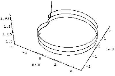
Figure 1: The bifurcation solution of the equation (2).

A description of the internal asymptotic structure of the solution in the case of the hard loss of the stability is connected with a construction of the asymptotics for the solution of the Painlevé-1 equation [5]. Besides the solution has a complicated asymptotic structure in the transition layer where the main term of the asymptotics is defined by four various expansions of different types. There are: a special solution of the Painlevé-1 equation, a sequence of separatrix solutions of the homogeneous equation with ”frozen” coefficients, a sequence of solutions of the Weierstrass equation with the parameter $g_{2}=0$ and a sequence of solutions of the Weierstrass equation with the parameter $g_{2}\not=0$.

Two of the first internal layers were found and studied in [5]. Later, in [6], [7] the asymptotic structure of the transition layer was studied in detail. It was shown that actually it is necessary to study the sequence of the separatrix solutions of the homogeneous equation with ”frozen” coefficients. The third internal layer was found in [7].

However, these three layers are not enough for a passage through the bifurcation interval. There exists a layer which is defined by a solution of the Weierstrass equation with the parameter $g_{2}\not=0$. This layer is found and studied in this work due to the matching of all asymptotic solutions before inside and after the bifurcation layer. The another new result of this paper is the calculating of internal variables in a sequence of layers, which are connected with the separatrix solutions of the homogeneous equation with ”frozen” coefficients. For the Painlevé-2 equation with a small parameter at a derivative these calculations have been made in the work of one of the authors of this paper in [8].

Among other works devoted to the investigation of the asymptotics solutions for nonlinear differential equations with variable coefficients it is necessary to note the investigations of passage through a separatrix in [9] -[12], where there were no confluent of the slowly varying equilibrium. In particular, in work [12] the passage through a separatrix of equation (2) with constant coefficients and small dissipation was studied. In the case considered in this work the solution of the equation for the amplitude also passes through a separatrix, but at more complicated confluent saddle-center equilibrium.

Here, the asymptotic solution for the equation (1) in the domain where the amplitude varies slowly ($t>t_{*}$) is constructed by perturbation theory method and in domain where the amplitude fast oscillates — by the Krylov-Bogolyubov method [1, 14]. Thus, we reproduce the elegant formulas for the asymptotic solutions of the equation (1) obtained in the work [15]. All asymptotics are matched [16].

The structure of this paper is following. In the second section the problem is formulated. In the third one, the obtained results are represented. The fourth section is devoted to a construction of an algebraic asymptotic solution for the equation (2). The fifth section includes an investigation of a bifurcation layer and studying of the sequences of the internal expansions. In the sixth section the fast oscillating solution of the equation (2) is constructed and its asymptotics at the approach to a bifurcation point is written.

2 Studied problem and its justification

2.1 Justification

The general solution of the equation (1) generally speaking is unknown. But we can construct a set of formal asymptotic solutions on a small parameter $\varepsilon$. The simplest kind of the solutions is the solutions oscillating with the frequency of the external force. To obtain this kind of solutions it is necessary to proceed the amplitude equation (2). Further following the natural suggestion about boundedness of the derivative in the equation (2) we can obtain a nonlinear algebraic equation for the main term of asymptotics $\stackrel{{\scriptstyle 0}}{{U}}(t)$:

$$|\stackrel{{\scriptstyle 0}}{{U}}|^{2}\stackrel{{\scriptstyle 0}}{{U}}-t\stackrel{{\scriptstyle 0}}{{U}}=1.$$ (3)

The number of the roots of this algebraic equation depends on a parameter $t$. The roots can be written explicitly. There exist a value of the parameter $t$ equals to $t_{*}=3(1/2)^{2/3}$ so that the equation (3) has three real roots at $t>t_{*}$. At $t=t_{*}=3(1/2)^{2/3}$ there is one simple root and one multiple root $U_{*}=-(1/2)^{1/3}$. At $t<t_{*}$ the equation (3) has the alone root.

Let us consider the domain $t>t_{*}$ where there are three different roots of the equation (3). Denote them $U_{k}$, and $U_{3}(t)<U_{2}(t)<U_{1}(t)$. These roots correspond to slowly varying equilibriums of the equation (2). Two of the equilibriums are stable centers. The formal asymptotic solutions with the main terms $U_{1}(t),\,U_{2}(t)$ correspond to these stable equilibriums. The third equilibrium is a saddle. There exists a parameter value $t=t_{*}$ at which one of the centers coalesces with the saddle. At that moment the saddle-center bifurcation takes place. At $t<t_{*}$ there exists only one slowly varying equilibrium.

This bifurcation may by explained on the example of an autonomous equation with a ”frozen” coefficient $T$:

$$iV^{\prime}+(|V|^{2}-T)V=1.$$

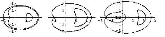
Figure 2: The phase portraits for the equations with the ”frozen” coefficient at $T<t_{*}$, $T=t_{*}$ and $T>t_{*}$.

On the figure 2 one can see the phase plane of this equation. On the left picture one equilibrium exists. On the middle picture one can find two equilibrium positions and at last on the right picture one can find three equilibrium positions.

Choosing $U_{k}$ as the main term of the asymptotics in the domain $t>t_{*}$ one can construct three different formal asymptotic solutions in the form:

$$U(t;\varepsilon)=\sum_{n=0}^{\infty}\varepsilon^{n}\stackrel{{\scriptstyle n}}{{U}}(t).$$ (4)

Each of them corresponds to the one of the slowly varying equilibrium. The formal solution with the main term $U_{1}(t)$ doesn’t change the structure when the variable $t$ changes and we do not investigate this case. Solution based on $U_{3}(t)$ is unstable on the whole interval $t>t_{*}$ and it is also out of our consideration. We will investigate the asymptotic solution based on $U_{2}(t)$ and the behavior of this asymptotic solution after the saddle-center bifurcation.

2.2 Statement of the problem

In this work we solve the problem on constructing of the formal asymptotic solution of the equation (1) in the interval $t\in[t_{*}-C,t_{*}+C]$ where $C=\hbox{const}>0$ uniform on $\varepsilon$ . We suppose that the solution in the domain $t>t_{*}$ has the form

$$\psi(t,\varepsilon)=\exp\bigg{(}{it^{2}\over 2\varepsilon}\bigg{)}\sum_{n=0}^{\infty}\varepsilon^{n}\stackrel{{\scriptstyle n}}{{U}}(t),\quad\varepsilon\to 0,$$

where $\stackrel{{\scriptstyle 0}}{{U}}(t)=U_{2}(t)$.

3 Result

The combined asymptotic solution of the equation (1) in an interval $t\in[t_{*}-C,t_{*}+C]$ is constructed. The solution has the different asymptotic structure in different parts of the interval. The main result of this work is following: firstly, the domain where constructed combined solution is valid completely covers the interval $[t_{*}-C,t_{*}+C]$ and secondly, all asymptotics are matched. In this section we only represent the form of asymptotics and leader terms. The explicit formulas can be found in the corresponding sections of the paper.

In the domain $(t-t_{*})\varepsilon^{-4/5}\gg 1$ the asymptotic solution has the form:

$$\psi(t,\varepsilon)=\exp\bigg{(}{it^{2}\over 2\varepsilon}\bigg{)}\sum_{n=0}^{\infty}\varepsilon^{n}\stackrel{{\scriptstyle n}}{{U}}(t),\quad\varepsilon\to 0.$$

The leader term of the asymptotics is equal to the middle root of algebraic equation (3): $\stackrel{{\scriptstyle 0}}{{U}}(t)=U_{2}(t)$. The correction terms $\stackrel{{\scriptstyle n}}{{U}}(t)$ are algebraic functions of $t$.

In the domain $|t-t_{*}|\ll 1$ the asymptotic solution is defined by four various expansions of different types. First of them is:

$$\psi=\bigg{(}U_{*}+\varepsilon^{2/5}\sum_{n=0}^{\infty}\varepsilon^{2n/5}\stackrel{{\scriptstyle n}}{{\alpha}}(\tau)+i\varepsilon^{3/5}\sum_{n=0}^{\infty}\varepsilon^{2n/5}\stackrel{{\scriptstyle n}}{{\beta}}(\tau)\bigg{)}\exp\bigg{(}{it^{2}\over 2\varepsilon}\bigg{)},\quad\varepsilon\to 0,$$ (5)

where $U_{*}$ is multiple root of the cubic equation (3) at $t=t_{*}$. The coefficients of this expansion depend on new scaling time $\tau=(t-t_{*})\varepsilon^{-4/5}$. The leader term of the asymptotics and the corrections are defined by their asymptotics as $\tau\to-\infty$ uniquely. In particular, the leader term of asymptotics $\stackrel{{\scriptstyle 0}}{{\alpha}}(\tau)$ is a special solution of the Painlevé-1 equation:

$$\stackrel{{\scriptstyle 0}}{{\alpha}}{}^{\prime\prime}-3\stackrel{{\scriptstyle 0}}{{\alpha}}\!\!^{2}+\tau=0.$$

with the given asymptotics as $\tau\to-\infty$:

$$\stackrel{{\scriptstyle 0}}{{\alpha}}(\tau)=\sum_{n\geq 0}\alpha_{n}\tau^{-{{(5n-1)}\over 2}},\quad{\hbox{where}}\,\,\,\,\alpha_{0}={1\over\sqrt{3}},\,\,\alpha_{1}={1\over 24}.$$

In the domain $\tau>-\infty$ this solution has poles on the real axis of $\tau$. Denote the least of them by $\tau_{0}$. The asymptotics (5) is valid as $(\tau-\tau_{0})\varepsilon^{-1/5}\gg 1$.

In the neighborhood of the bifurcation point $(\tau=\tau_{0})$ the coefficients of the asymptotic expansion depend on one more fast time scale $\theta=(\tau-\tau_{0})\varepsilon^{-1/5}$. Denote by

$$\theta_{0}=\theta+\sum_{n=1}^{\infty}\varepsilon^{n/5}\stackrel{{\scriptstyle n}}{{\theta}}_{0},$$

where $\stackrel{{\scriptstyle n}}{{\theta}}_{0}=\hbox{const}$. Then in the domain $-\varepsilon^{-1/5}\ll\theta_{0}\ll\varepsilon^{-1/10}$ the formal asymptotic solution has the form:

$$\psi(t,\varepsilon)=\bigg{(}U_{*}+\stackrel{{\scriptstyle 0}}{{w}}(\theta_{0})+\varepsilon^{4/5}\sum_{n=1}^{\infty}\varepsilon^{(n-1)/5}\stackrel{{\scriptstyle n}}{{w}}(\theta_{0})\bigg{)}\exp\bigg{(}{it^{2}\over 2\varepsilon}\bigg{)},\quad\varepsilon\to 0.$$

The main term of asymptotics $\stackrel{{\scriptstyle 0}}{{w}}(\theta_{0})$ is the separatrix solution of the autonomous equation:

$$i\stackrel{{\scriptstyle 0}}{{w}}{}^{\prime}+U_{*}\left(2|\stackrel{{\scriptstyle 0}}{{w}}|^{2}+\stackrel{{\scriptstyle 0}}{{w}}\!{}^{2}\right)+U_{*}^{2}\left(\stackrel{{\scriptstyle 0}}{{w}}\!^{*}-\stackrel{{\scriptstyle 0}}{{w}}\right)+|\stackrel{{\scriptstyle 0}}{{w}}|^{2}\stackrel{{\scriptstyle 0}}{{w}}=0,$$ (6)

namely:

$$\stackrel{{\scriptstyle 0}}{{w}}(\theta_{0})={{-2}\over{(\theta_{0}-iU_{*})^{2}}}.$$

In the domain $-\theta_{0}\gg 1$ the asymptotic solution is defined by a sequence of two alternating asymptotics. Let us call them by ”intermediate” and ”separatrix” asymptotics. To obtain the intermediate asymptotics let us introduce one more slow variable:

$$T_{k}=\theta_{k-1}\varepsilon^{1/6},k=1,2,\dots.$$

An asymptotic solution in the intermediate domain for not too large values $k$:

$$k\ll\varepsilon^{-1/7}$$

has the form:

$$\psi(t,\varepsilon)=\bigg{(}U_{*}+\varepsilon^{1/3}\sum_{n=0}^{\infty}\varepsilon^{1/30}\stackrel{{\scriptstyle n}}{{A}}_{k}(T_{k})\,+\,$$

$$i\varepsilon^{1/2}\sum_{n=0}^{\infty}\varepsilon^{1/30}\stackrel{{\scriptstyle n}}{{B}}_{k}(T_{k})\bigg{)}\exp\bigg{(}{it^{2}\over 2\varepsilon}\bigg{)},\quad\varepsilon\to 0.$$

The leader term of the asymptotics satisfies to the equation:

$$\stackrel{{\scriptstyle 0}}{{A}}_{k}\!\!\!^{\prime\prime}+3\stackrel{{\scriptstyle 0}}{{A}}_{k}\!\!\!^{2}=0$$

and can be expressed by the Weierstrass function with the parameter $g_{2}=0$:

$$\stackrel{{\scriptstyle 0}}{{A}}_{k}=-2\wp(T_{k};0,g_{3}(k)),\,\,\,\hbox{where}\,\,\,g_{3}(k)={1\over 56}\big{(}g_{3}(k-1)+\pi/2\big{)},\,\,\,g_{3}(0)={a_{4}\over 56}.$$ (7)

The constant $a_{4}$ is the coefficient as $(\tau-\tau_{0})^{4}$ in the Laurent expansion of $\stackrel{{\scriptstyle 0}}{{\alpha}}(\tau)$.

The Weierstrass $\wp$-function has a real period $\Omega_{k}$ and has poles on the real axis at $T_{k}=0$ and $T_{k}=\Omega_{k}$. The intermediate expansion with the leader term (7) is valid in the domain between the poles as

$$-\varepsilon^{-1/6}T_{k}\gg 1,\quad\varepsilon^{-2/15}(T_{k}+\Omega_{k})\gg 1.$$

At the large values of $k$ the intermediate asymptotics are constructed in the form

$$\psi(t,\varepsilon)=\bigg{(}U_{*}+\varepsilon^{1/3}\sum_{n=0}^{\infty}\varepsilon^{n/6}\stackrel{{\scriptstyle 5n}}{{A}}_{k}(T_{k})\,+\,$$

$$i\varepsilon^{1/2}\sum_{n=0}^{\infty}\varepsilon^{n/6}\stackrel{{\scriptstyle 5n}}{{B}}_{k}(T_{k})\bigg{)}\exp\bigg{(}{it^{2}\over 2\varepsilon}\bigg{)},\quad\varepsilon\to 0.$$

The leader term of asymptotics satisfies to the equation:

$$\stackrel{{\scriptstyle 0}}{{A}}_{k}^{\prime\prime}+3\stackrel{{\scriptstyle 0}}{{A}}_{k}\!\!\!^{2}=\lambda_{k}.$$

$$\lambda_{k}(\varepsilon)=\varepsilon^{1/6}\bigg{(}\sum_{j=1}^{k}\Omega_{j}\,+\,\sum_{n=1}^{\infty}\varepsilon^{(n-1)/30}\sum_{j=1}^{k}\stackrel{{\scriptstyle n}}{{x}}_{j}\!\!\!^{+}\bigg{)}.$$

The main term of the asyptotics is:

$$\stackrel{{\scriptstyle 0}}{{A}}_{k}(T_{k})=-2\wp(T_{k},\lambda_{k}/2,g_{3}(k,\varepsilon)),$$ (8)

where

$$g_{3}(k,\varepsilon)=\stackrel{{\scriptstyle 0}}{{g}}_{3}(k)+\sum_{n=1}^{\infty}\varepsilon^{n/30}\stackrel{{\scriptstyle n}}{{g}}_{3}(k).$$

The intermediate expansion with the leader term (8) is valid in the domain between the poles of the Weierstrass function as

$$-\varepsilon^{-1/6}T_{k}\gg 1,\quad\varepsilon^{-2/15}(T_{k}+\Omega_{k})\gg 1.$$

The separatrix expansions are valid in a small neighborhood of the Weierstrass function poles. Denote:

$$\theta_{k}=\big{(}T_{k}+\Omega_{k}-{1\over 4}\sum_{n=1}^{\infty}\varepsilon^{n/30}\stackrel{{\scriptstyle n}}{{x}}_{k}\!\!\!^{+}\big{)}\varepsilon^{-1/6},\quad k=1,2,\dots.$$

When

$$|\theta_{k}|\varepsilon^{1/6}\ll 1$$

the formal asymptotic solution of equation (1) has the form:

$$\psi=\bigg{(}U_{*}+\stackrel{{\scriptstyle 0}}{{W}}(\theta_{k})+\varepsilon^{4/5}\sum_{n=1}^{\infty}\varepsilon^{(n-1)/30}\stackrel{{\scriptstyle n}}{{W}}(\theta_{k})\bigg{)}\exp\bigg{(}{it^{2}\over 2\varepsilon}\bigg{)}\quad\varepsilon\to 0.$$

The leader term of the asymptotics $\stackrel{{\scriptstyle 0}}{{W}}(\theta_{k})$ is a separatrix solution of the autonomous equation (6):

$$\stackrel{{\scriptstyle 0}}{{W}}(\theta_{k})={{-2}\over{(\theta_{k}-iU_{*})^{2}}}.$$

The sequence of the alternating intermediate expansions and separatrix asymptotic ones is valid as $\varepsilon^{-1/6}(t_{*}-t)\ll 1$.

In the domain $(t_{*}-t)\varepsilon^{-2/3}\gg 1$ the asymptotic solution becomes two-phase. The amplitude of the stimulated oscillations in the solution of (1) oscillates fast. The form of the solution is:

$$\psi=\bigg{(}\stackrel{{\scriptstyle 0}}{{U}}(t_{1},t,\varepsilon)+\varepsilon\stackrel{{\scriptstyle 1}}{{U}}(t_{1},t,\varepsilon)+\varepsilon^{2}\stackrel{{\scriptstyle 2}}{{U}}(t_{1},t,\varepsilon)\bigg{)}\exp\bigg{(}{it^{2}\over\varepsilon}\bigg{)},$$

where $t_{1}$ is a new fast variable $t_{1}=S(t)/\varepsilon+\phi(t)$. The main term of the asymptotics $\stackrel{{\scriptstyle 0}}{{U}}$ lies on the curve $\Gamma(t)$:

$${1\over 2}|y|^{4}-t|y|^{2}-(y+\bar{y})=E(t),$$

and satisfies to the Cauchy problem for the equation

$$iS^{\prime}\partial_{t_{1}}\stackrel{{\scriptstyle 0}}{{U}}=\pm\sqrt{2\stackrel{{\scriptstyle 0}}{{U}}\!^{3}+(2E(t)+t^{2})\stackrel{{\scriptstyle 0}}{{U}}\!^{2}+2t\stackrel{{\scriptstyle 0}}{{U}}+1},$$

with an initial condition $\stackrel{{\scriptstyle 0}}{{U}}|_{t_{1}=0}=u_{0}$, such, that $\Im(u_{0})=0,\quad\Re(u_{0})=\min_{y\in\Gamma(t)}\big{(}\Re(y)\big{)}$. The function $S(t)$ is a solution for the Cauchy problem

$$iS^{\prime}\int_{\Gamma(t)}{dy\over\sqrt{3y^{3}+(2E+t^{2})y^{2}+2ty+1}}=T,S|_{t=0}=0,$$

where $T=\hbox{const}>0$. The function $E(t)$ is the solution of the transcendental equation

$$i\int_{\Gamma(t)}u^{*}du=\pi.$$

The phase shift $\phi$ is defined by two constant. One of them is an ”initial” condition $\phi(t_{*})=\phi_{0}$ and another one is a constant $\phi_{1}$ in the equation in for $\phi$:

$${\phi^{\prime}\over\partial_{E}S}\partial_{E}I=\phi_{1}.$$

Remark 1

In our work constants $\phi_{0}$ and $\phi_{1}$ are not calculated. It means that the phase shift of the fast oscillating asymptotics remains to be undefined. Its evaluation within the framework of our approach requires an evaluation on an explicit form of the asymptotics of the higher corrections in the internal expansions at their matching with the fast oscillating asymptotics.

4 Construction of an algebraic asymptotics

In this section the formal asymptotic solution for the equation (2) has been constructed in the form of series on integer powers of the small parameter $\varepsilon$. We show that this expansion is valid in the interval $(t-t_{*})\varepsilon^{-4/5}\gg 1$.

The coefficients of this asymptotics are defined from the recurrent sequence of algebraic equations. These equations can be obtained by substituting of the series (4) in the equation (2) and by collecting of the terms under the same powers of the small parameter. In particular, the algebraic equation (3) for the leader term of the asymptotics can be obtained from the relation under $\varepsilon^{0}$.

Further we will use the root $U_{2}(t)$ as the main term $\stackrel{{\scriptstyle 0}}{{U}}(t)$ of the asymptotics (4). It means that we investigate the formal asymptotics (4) corresponding to the stable center which converges with the saddle at $t_{*}$.

The relation under $\varepsilon^{1}$ give us the equations for real and imaginary parts of the first correction term $\stackrel{{\scriptstyle 1}}{{U}}=u_{1}+iv_{1}$

$$[3\stackrel{{\scriptstyle 0}}{{U}}\!^{2}-t]u_{1}=0,\quad[\stackrel{{\scriptstyle 0}}{{U}}\!^{2}-t]v_{1}=-\partial_{t}\stackrel{{\scriptstyle 0}}{{U}}.$$ (9)

The expression $[3\stackrel{{\scriptstyle 0}}{{U}}\!^{2}-t]$ vanishes at $t=t_{*}$. So it is easy to obtain that the even corrections are real, and the odd corrections are imaginary.

The explicit form of the first correction is:

$$\stackrel{{\scriptstyle 1}}{{U}}=-{i\,{\stackrel{{\scriptstyle 0}}{{U}}}\over{[3\stackrel{{\scriptstyle 0}}{{U}}\!^{2}-t][\stackrel{{\scriptstyle 0}}{{U}}\!^{2}-t]}}.$$ (10)

This expression has a singularity at $t=t_{*}$. The order of the singularity increases with respect to the number of the corrections of the asymptotics as $t\to t_{*}$. In the neighborhood of the point $t_{*}$ the coefficients of asymptotics (4) have the form:

in the case of $n=0,1$:

$$\stackrel{{\scriptstyle n}}{{U}}(t)=(t-t_{*})^{-n/2}\sum_{k=0}^{\infty}\stackrel{{\scriptstyle n}}{{U}}_{k}(t-t_{*})^{k/2},$$ (11)

where $\stackrel{{\scriptstyle 0}}{{U}}_{0}=U_{*}$, $\stackrel{{\scriptstyle 0}}{{U}}_{1}=1/\sqrt{3}$;

in the case of $m=2n,\,\,m=2n+1$, $n\in\hbox{\Sets N}$:

$$\stackrel{{\scriptstyle m}}{{U}}(t)=(t-t_{*})^{(1-5m)/2}\sum_{k=0}^{\infty}\stackrel{{\scriptstyle m}}{{U}}_{k}(t-t_{*})^{k/2}.$$ (12)

The increasing of the singularity of the corrections in (4) makes this expansion unusable as $t\to t_{*}$. The singularities of the coefficients define the domain of the suitability for the formal asymptotic solution (4) as $(t-t_{*})\varepsilon^{-4/5}\gg 1$.

5 Expansions in bifurcation layer

In this section the formal asymptotic solution for equation (2) has been constructed in the domain $|t-t_{*}|\ll 1$. Usually the asymptotics of this type is called internal ones [16].

5.1 Initial interval

5.1.1 The first internal expansion — Painlevé-1 interval

In the neighborhood of the singularity we will use a new scaling variable $\tau=(t-t_{*})\varepsilon^{-4/5}$. This new variable $\tau$ is defined by the structure of external asymptotic solution (4) singularities.

We will construct the solution of the original equation (2) in the form:

$$U=U_{*}+\varepsilon^{2/5}\alpha(\tau,\varepsilon)+i\varepsilon^{3/5}\beta(\tau,\varepsilon),$$ (13)

The equations for $\alpha$ and $\beta$ are

$$\alpha^{\prime}+(U_{*}^{2}-t_{*})\beta=-\varepsilon^{2/5}2U_{*}\alpha\beta\,-\,\varepsilon^{4/5}(\alpha^{2}-\tau)\beta\,-\,\varepsilon^{6/5}\beta^{3},$$

$$\beta^{\prime}-3U_{*}\alpha^{2}+U_{*}\tau=\varepsilon^{2/5}(-\alpha^{3}-U_{*}\beta^{2}+\alpha\tau)\,+\,\varepsilon^{4/5}\alpha\beta^{2}.$$ (14)

The asymptotics of the functions $\alpha$ and $\beta$ as $\tau\to\infty$ is known. It can be obtained by substituting (11) and (12) in formula (4) and by decomposing of this expression in the terms of the scaling variable $\tau$:

$$\alpha(\tau,\varepsilon)={1\over\sqrt{3}}\sqrt{\tau}+\sum_{n=1}^{\infty}\tau^{(1-5n)/2}\stackrel{{\scriptstyle 2n}}{{U}}_{0}+\varepsilon^{2/5}\sum_{n=0}^{\infty}\stackrel{{\scriptstyle 2n}}{{U}}_{1}\tau^{(2-5n)/2}+$$

$$\varepsilon^{4/5}\sum_{n=0}^{\infty}\stackrel{{\scriptstyle 2n}}{{U}}_{2}\tau^{(3-5n)/2}+\dots.$$ (15)

$$\beta(\tau,\varepsilon)={1\over\sqrt{\tau}}\stackrel{{\scriptstyle 1}}{{U}}_{0}+\sum_{n=1}^{\infty}\stackrel{{\scriptstyle 2n+1}}{{U}}\!\!\!\!_{0}\,\,\tau^{-(1+5n)/2}\,+\,\varepsilon^{2/5}\sum_{n=0}^{\infty}\stackrel{{\scriptstyle 2n+1}}{{U}}\!\!\!\!_{1}\,\,\tau^{-(2-5n)/2}+\dots.$$ (16)

It is convenient to construct the solution of the equations (14) in the form of formal series on powers of the small parameter $\varepsilon$:

$$\alpha(\tau,\varepsilon)=\sum_{n=0}^{\infty}\varepsilon^{2n/5}\stackrel{{\scriptstyle n}}{{\alpha}}(\tau),\quad\beta(\tau,\varepsilon)=\sum_{n=0}^{\infty}\varepsilon^{2n/5}\stackrel{{\scriptstyle n}}{{\beta}}(\tau).$$ (17)

The leader correction terms are defined by the system of ordinary differential equations

$$\stackrel{{\scriptstyle 0}}{{\alpha}}\!^{\prime}+(U_{*}^{2}-t_{*})\stackrel{{\scriptstyle 0}}{{\beta}}=0,$$ (18)

$$\stackrel{{\scriptstyle 0}}{{\beta}}\!^{\prime}-3U_{*}\stackrel{{\scriptstyle 0}}{{\alpha}}\!\!^{2}+\tau U_{*}=0.$$ (19)

Let us differentiate the first equation and take into account that $U_{*}(U_{*}^{2}-t_{*})=1$ then we obtain the Painlevé-1 equation for $\stackrel{{\scriptstyle 0}}{{\alpha}}$

$$\stackrel{{\scriptstyle 0}}{{\alpha}}{}^{\prime\prime}-3\stackrel{{\scriptstyle 0}}{{\alpha}}\!\!^{2}+\tau=0.$$ (20)

Matching the asymptotics (13), (17) and asymptotics (4) as $t\to t_{*}+0$ we obtain the asymptotic structure of $\stackrel{{\scriptstyle 0}}{{\alpha}}(\tau)$ as $\tau\to+\infty$

$$\stackrel{{\scriptstyle 0}}{{\alpha}}(\tau)=\sum_{n\geq 0}\alpha_{n}\tau^{-{{(5n-1)}\over 2}},\quad{\hbox{where}}\,\,\,\,\alpha_{0}={1\over\sqrt{3}},\,\,\alpha_{1}={1\over 24}.$$ (21)

The solution of the Painleve-1 equation with the asymptotics of (21) was investigated in [17, 18].

The coefficients of the formal expansion (17) for the function $\beta$ can be obtained from the first equation of the system (14). In particular:

$$\stackrel{{\scriptstyle 0}}{{\beta}}={\stackrel{{\scriptstyle 0}}{{\alpha}}\!^{\prime}\over 2U_{*}^{2}},\quad\stackrel{{\scriptstyle 1}}{{\beta}}={1\over 2U_{*}^{2}}\bigg{(}\stackrel{{\scriptstyle 1}}{{\alpha}}\!^{\prime}+2U_{*}\stackrel{{\scriptstyle 0}}{{\alpha}}\stackrel{{\scriptstyle 0}}{{\beta}}\bigg{)},$$

$$\stackrel{{\scriptstyle 2}}{{\beta}}={1\over 2U_{*}^{2}}\bigg{(}\stackrel{{\scriptstyle 2}}{{\alpha}}\!^{\prime}+\stackrel{{\scriptstyle 0}}{{\alpha}}\!^{2}\stackrel{{\scriptstyle 0}}{{\beta}}+2U_{*}\stackrel{{\scriptstyle 1}}{{\alpha}}\stackrel{{\scriptstyle 0}}{{\beta}}+2U_{*}\stackrel{{\scriptstyle 0}}{{\alpha}}\stackrel{{\scriptstyle 1}}{{\beta}}-\tau\stackrel{{\scriptstyle 0}}{{\beta}}\bigg{)}.$$

The equation for the first correction term $\stackrel{{\scriptstyle 1}}{{\alpha}}(\tau)$ has the form

$$\stackrel{{\scriptstyle 1}}{{\alpha}}{}^{\prime\prime}+6U_{*}(U_{*}^{2}-t_{*})\stackrel{{\scriptstyle 0}}{{\alpha}}\stackrel{{\scriptstyle 1}}{{\alpha}}+2U_{*}(U_{*}^{2}-t_{*})\stackrel{{\scriptstyle 0}}{{\beta}}\!{}^{2}+(U_{*}^{2}-t_{*})\stackrel{{\scriptstyle 0}}{{\alpha}}\!{}^{3}-(U_{*}^{2}-t_{*})\stackrel{{\scriptstyle 0}}{{\alpha}}\tau=$$

$$-2U_{*}\stackrel{{\scriptstyle 0}}{{\alpha}}{}^{\prime}\stackrel{{\scriptstyle 0}}{{\beta}}-2U_{*}\stackrel{{\scriptstyle 0}}{{\alpha}}\stackrel{{\scriptstyle 0}}{{\beta}}{}^{\prime}.$$ (22)

The asymptotics of a solution for this equation is uniquely defined by matching of the asymptotics of the external expansion (4) and internal expansion (13), (17):

$$\stackrel{{\scriptstyle 1}}{{\alpha}}=\stackrel{{\scriptstyle 0}}{{U}}_{2}\tau-\stackrel{{\scriptstyle 2}}{{U}}_{6}\tau^{-3/2}+O(\tau^{-4}),\quad\tau\to+\infty$$ (23)

A simple calculation gives us the domain of a suitability of that asymptotic expansion. The representation (17) of the solution is valid as $\tau\ll\varepsilon^{-4/5}$. This result is similar to [5].

It is known that the solution of the Painlevé-1 equation with the asymptotics (21) has poles at points $\tau_{k}$ [19]. Let us denote the first pole by $\tau_{0}$ and call it the point of the bifurcation.

The solution of the Painlevé-1 equation is represented by converging series in the neighborhood of the point $\tau_{0}$ [18]:

$$\stackrel{{\scriptstyle 0}}{{\alpha}}(\tau)=-{2\over{(\tau-\tau_{0})^{2}}}-{\tau_{0}\over 10}(\tau-\tau_{0})^{2}+a_{4}(\tau-\tau_{0})^{4}+\sum_{k=6}^{\infty}\stackrel{{\scriptstyle 0}}{{\alpha}}_{k}(\tau-\tau_{0})^{k},$$

the constants $\tau_{0}$ and $a_{4}$ are parameters of the solution.

The first correction term $\stackrel{{\scriptstyle 1}}{{\alpha}}$ is defined by the equation (22) and asymptotics (23). In the neighborhood of the bifurcation point $\tau_{0}$ as $\tau>\tau_{0}$ the function $\stackrel{{\scriptstyle 1}}{{\alpha}}$ is represented in the form:

$$\stackrel{{\scriptstyle 1}}{{\alpha}}=\stackrel{{\scriptstyle 1}}{{\alpha}}_{c}(\tau)+\stackrel{{\scriptstyle 1}}{{a}}\!^{+}\alpha_{1}(\tau)+\stackrel{{\scriptstyle 1}}{{b}}\!^{+}\alpha_{2}(\tau).$$ (24)

Where $\stackrel{{\scriptstyle 1}}{{\alpha}}_{c}(\tau)$ is the partial solution of the nonhomogeneous equation for the function $\stackrel{{\scriptstyle 1}}{{\alpha}}(\tau)$ with the asymptotics:

$$\stackrel{{\scriptstyle 1}}{{\alpha}}_{c}(\tau)=\stackrel{{\scriptstyle 1}}{{\alpha}}_{-4}(\tau-\tau_{0})^{-4}+\sum_{k=0}^{\infty}\stackrel{{\scriptstyle 1}}{{\alpha}}_{k}(\tau-\tau_{0})^{k},\quad\stackrel{{\scriptstyle 1}}{{\alpha}}_{-4}={1\over{U_{*}^{7}}},\quad\stackrel{{\scriptstyle 1}}{{\alpha}}_{4}=0.$$

It is convenient to use the partial solution with the coefficients as $(\tau-\tau_{0})^{-3}$ and $(\tau-\tau_{0})^{4}$ equal to zero.

The constants $\stackrel{{\scriptstyle 1}}{{a}}\!^{+}$ and $\stackrel{{\scriptstyle 1}}{{b}}\!^{+}$ in the formula (24) can be uniquely defined by asymptotics of $\stackrel{{\scriptstyle 1}}{{\alpha}}$ as $\tau\to\infty$. The functions $\alpha_{1}(\tau)$ and $\alpha_{2}(\tau)$ are linear independent solutions of the homogeneous equation for $\stackrel{{\scriptstyle 1}}{{\alpha}}(\tau)$. These functions are uniquely defined by their asymptotics as $\tau\to\tau_{0}$:

$$\alpha_{1}(\tau)=(\tau-\tau_{0})^{-3}+a_{1}(\tau-\tau_{0})+a_{2}(\tau-\tau_{0})^{2}+a_{3}(\tau-\tau_{0})^{3}+O((\tau-\tau_{0})^{5}),$$

where $a_{n}=\hbox{const}$;

$$\alpha_{2}(\tau)=(\tau-\tau_{0})^{4}+O((\tau-\tau_{0})^{8}).$$

The next correction terms are represented by the following formula:

$$\stackrel{{\scriptstyle n}}{{\alpha}}(\tau)=\stackrel{{\scriptstyle n}}{{\alpha}}_{c}(\tau)+\stackrel{{\scriptstyle n}}{{a}}\!^{+}\alpha_{1}(\tau)+\stackrel{{\scriptstyle n}}{{b}}\!^{+}\alpha_{2}(\tau).$$

The partial solution $\stackrel{{\scriptstyle n}}{{\alpha}}_{c}(\tau)$ of the equation has the asymptotics as $\tau\to\tau_{0}$:

$$\stackrel{{\scriptstyle n}}{{\alpha}}_{c}(\tau)=\stackrel{{\scriptstyle n}}{{\alpha}}_{-2n}(\tau-\tau_{0})^{-2n}+\dots,$$

where dots mean the terms of the next orders on $(\tau-\tau_{0})$.

It is convenient for us to denote the partial solution which does not contain terms of the order of $(\tau-\tau_{0})^{-3}$ and $(\tau-\tau_{0})^{4}$ in the asymptotics as $\tau\to\tau_{0}$ by $\stackrel{{\scriptstyle n}}{{\alpha}}_{c}(\tau)$.

By analysis of written asymptotics we obtain that the formal asymptotic solution (13) is valid as $(\tau-\tau_{0})\varepsilon^{-1/5}\gg 1$.

5.1.2 The second internal expansion, the neighborhood of the bifurcation point

In this section we construct the formal asymptotic solution for the equation (2), which is valid in the neighborhood of the bifurcation point $|\tau-\tau_{0}|\ll 1$.

The domain where the first asymptotic expansion is valid determines the second internal scale. We will use a new scaling variable $\theta=(\tau-\tau_{0})\varepsilon^{-1/5}$ in the small neighborhood of the point $\tau_{0}$.

We change the unknown function in the equation (2) and pass to the function $w=U-U_{*}$.

Substituting the expressions for $w$ and $\theta$ in the original problem we obtain the equation for $w(\theta,\varepsilon)$

$$iw^{\prime}+2U_{*}^{2}w+2U_{*}|w|^{2}+|w|^{2}w+U_{*}^{2}w^{*}+U_{*}w^{2}-$$

$$-\varepsilon^{4/5}\tau_{0}\big{(}U_{*}+w\big{)}-\varepsilon\theta\big{(}U_{*}+w\big{)}=0.$$ (25)

The asymptotics of the function $w(\theta,\varepsilon)$ as $\theta\to+\infty$ can be obtained by expansing in series of the function $U=U_{*}+\varepsilon^{2/5}\alpha(\tau,\varepsilon)+i\varepsilon^{3/5}\beta(\tau,\varepsilon)$ on variable $\theta$:

$$w(\theta,\varepsilon)=\bigg{(}{1\over U_{*}^{3}\theta^{2}}+{i\over 2U_{*}^{5}\theta^{3}}+\dots\bigg{)}+\varepsilon^{1/5}\stackrel{{\scriptstyle 1}}{{a}}\!^{+}\bigg{(}\theta^{-3}+\dots\bigg{)}+$$

$$\varepsilon^{3/5}\stackrel{{\scriptstyle 2}}{{a}}\!^{+}\bigg{(}\theta^{-3}+\dots\bigg{)}+\varepsilon^{4/5}\bigg{(}{2U_{8}^{3}\tau_{0}\over 10}\theta^{2}+\dots\bigg{)}+\dots.$$ (26)

In this formula dots mean the terms of the lesser order (in brackets with respect to $\theta$ and out of them with respect to $\varepsilon$).

In this section the formal asymptotic solution for the equation (25) with the given asymptotics (26) as $\varepsilon\to 0$ has been constructed. We indicate the domain where this formal solution for the equation (25) is valid.

The first step of the formal solution construction for the equation (25) is a choice of an asymptotic sequence. This choice for the external and the first internal expansions was defined by the equation. In this case the asymptotics as $\theta\to+\infty$ gives us the asymptotic sequence on $\varepsilon^{1/5}$. But the equation shows, that the first order correction should satisfy to the homogeneous equation. In this case we can satisfy to the asymptotic condition as $\theta\to+\infty$ by constructing of the formal solution in the form:

$$w(\theta,\varepsilon)=\stackrel{{\scriptstyle 0}}{{w}}(\theta_{0})\,+\,\varepsilon^{4/5}\sum_{n=1}^{\infty}\varepsilon^{(n-1)/5}\stackrel{{\scriptstyle n}}{{w}}(\theta_{0}),\quad\varepsilon\to 0$$ (27)

where

$$\theta_{0}=\theta+\varepsilon^{1/5}\stackrel{{\scriptstyle 1}}{{\theta_{0}}}+\varepsilon^{3/5}\stackrel{{\scriptstyle 2}}{{\theta_{0}}}+\dots\quad\varepsilon\to 0.$$

The correction terms $\stackrel{{\scriptstyle n}}{{\theta}}$ are defined by the asymptotics of the formal solution as $\theta\to\infty$:

$$\stackrel{{\scriptstyle n}}{{\theta_{0}}}={\stackrel{{\scriptstyle n}}{{a}}\!\!^{+}\over 4}.$$

It is convenient to pass from the equation (25) to the equation with respect to the variable $\theta_{0}$:

$$iw^{\prime}+(2U_{*}^{2}-t_{*})w+2U_{*}|w|^{2}+|w|^{2}w+U_{*}^{2}w^{*}+U_{*}w^{2}=$$

$$\bigg{(}\varepsilon^{4/5}\tau_{0}+\varepsilon\theta_{0}-\varepsilon^{6/5}\stackrel{{\scriptstyle 1}}{{\theta}}_{0}-\varepsilon^{8/5}\stackrel{{\scriptstyle 2}}{{\theta}}_{0}-\dots\bigg{)}\big{(}U_{*}+w\big{)},\quad\varepsilon\to 0.$$ (28)

To construct the formal solution $w(\theta_{0},\varepsilon)$ we substitute the formal series (27) in the equation (28) and gather the terms of the same order on $\varepsilon$. Then we obtain the recurrent sequence of the equations for the leader term and the corrections of the asymptotics. The equation for the leader term is

$$i\stackrel{{\scriptstyle 0}}{{w}}{}^{\prime}+U_{*}\left(2|\stackrel{{\scriptstyle 0}}{{w}}|^{2}+\stackrel{{\scriptstyle 0}}{{w}}\!{}^{2}\right)+U_{*}^{2}\left(\stackrel{{\scriptstyle 0}}{{w}}\!^{*}-\stackrel{{\scriptstyle 0}}{{w}}\right)+|\stackrel{{\scriptstyle 0}}{{w}}|^{2}\stackrel{{\scriptstyle 0}}{{w}}=0.$$ (29)

The asymptotics of $\stackrel{{\scriptstyle 0}}{{w}}$ as $\theta_{0}\to\infty$ can be obtained from the asympotics of the function $w(\theta_{0},\varepsilon)$

$$\stackrel{{\scriptstyle 0}}{{w}}(\theta_{0})={1\over U_{*}^{3}\theta_{0}^{2}}+{i\over 2U_{*}^{5}\theta_{0}^{3}}+\dots.$$ (30)

To construct the leader term $\stackrel{{\scriptstyle 0}}{{w}}(\theta_{0})$ we take the conservation law for the equation (29):

$$U_{*}\left[|w|^{2}w^{*}+|w|^{2}w\right]+U_{*}^{2}\left[{1\over 2}(w^{*})^{2}+{1\over 2}w^{2}-|w|^{2}\right]+{1\over 2}|w|^{4}=H.$$

The constant $H$ for our solution is defined by asymptotics (30): $H=0$. Let us solve this formula for the function $w^{*}$ and substitute the representation over $w$ in the equation (29). Then we obtain

$$iw^{\prime}-2U_{*}w\sqrt{-U_{*}w}=0.$$ (31)

This equation can be obviously solved

$$\stackrel{{\scriptstyle 0}}{{w}}(\theta_{0})={{-2}\over{(\theta_{0}-iU_{*})^{2}}},$$ (32)

the integration constant is defined by the asymptotics (30). The leader term of the asymptotics (27) is the separatrix solution of the equation (29).

The next corrections $\stackrel{{\scriptstyle m}}{{w}},\,\,m=1,2\dots$ satisfy to the equations

$$i\stackrel{{\scriptstyle m}}{{w}}{}^{\prime}+\left[2U_{*}\stackrel{{\scriptstyle 0}}{{w}}\!^{*}+2U_{*}\stackrel{{\scriptstyle 0}}{{w}}-U_{*}^{2}+2\stackrel{{\scriptstyle 0}}{{w}}\stackrel{{\scriptstyle 0}}{{w}}\!^{*}\right]\stackrel{{\scriptstyle m}}{{w}}+\left(U_{*}+\stackrel{{\scriptstyle 0}}{{w}}\right)^{2}\stackrel{{\scriptstyle m}}{{w}}\!^{*}=\stackrel{{\scriptstyle m}}{{F}}.$$ (33)

In particular,

$$\stackrel{{\scriptstyle 1}}{{F}}=\tau_{0}(U_{*}+\stackrel{{\scriptstyle 0}}{{w}}),\quad\stackrel{{\scriptstyle 2}}{{F}}=\theta_{0}(U_{*}+\stackrel{{\scriptstyle 0}}{{w}})\quad\stackrel{{\scriptstyle 3}}{{F}}=-\stackrel{{\scriptstyle 1}}{{\theta_{0}}}(U_{*}+\stackrel{{\scriptstyle 0}}{{w}}),\quad\stackrel{{\scriptstyle 4}}{{F}}=0,$$

$$\stackrel{{\scriptstyle 5}}{{F}}=-\stackrel{{\scriptstyle 2}}{{\theta}}(U_{*}+\stackrel{{\scriptstyle 0}}{{w}})-2U_{*}|\stackrel{{\scriptstyle 1}}{{w}}|^{2}-U_{*}\stackrel{{\scriptstyle 1}}{{w}}\!\!^{2}.$$

The asymptotics $\stackrel{{\scriptstyle m}}{{w}}(\theta_{0})$ as $\theta\to\infty$ can be easy obtained from (26).

To construct the correction terms we need the solutions of the homogeneous equation (33). One of them can be obtained by differentiation with respect to variable $\theta_{0}$ of the function $\stackrel{{\scriptstyle 0}}{{w}}$

$$w_{1}(\theta_{0})={1\over 4}{d\over{d\theta_{0}}}\stackrel{{\scriptstyle 0}}{{w}}={1\over(\theta_{0}-iU_{*})^{3}}.$$ (34)

The formula for the second independent solution is complicated and we do not write it. The second solution grows as $|\theta|\to\infty$. The asymptotics as $\theta\to\infty$ of this solution has the form

$$w_{2}(\theta_{0})=\theta_{0}^{4}+i{1\over{2U_{*}^{2}}}\theta_{0}^{3}+\dots.$$ (35)

These independent solutions are such that their Wronskian is

$${\cal W}=w_{1}w_{2}^{*}-w_{2}w_{1}^{*}=-{7i\over U_{*}^{2}}.$$

By using the expressions for $w_{1}$ and $w_{2}$ we can write the next corrections for the asymptotic solution with the given asymptotics as $\theta_{0}\to+\infty$ in an explicit form. The asymptotics as $\theta_{0}\to-\infty$ of these corrections can be evaluated.

It is convenient for us to represent the higher corrections of the asymptotics (27) in the form

$$\stackrel{{\scriptstyle n}}{{w}}(\theta_{0})=\stackrel{{\scriptstyle n}}{{w}}_{c}(\theta_{0})+\stackrel{{\scriptstyle n}}{{X}}_{0}\!\!^{-}w_{1}(\theta_{0})+\stackrel{{\scriptstyle n}}{{Y}}_{0}\!\!^{-}w_{2}(\theta_{0}),$$ (36)

where, $\stackrel{{\scriptstyle n}}{{w}}_{c}(\theta_{0})$ is the partial solution for the n-th correction term and this solution does not contain terms of the order of $\theta_{0}^{4}$ and $\theta_{0}^{-3}$ in the asymptotics as $\theta_{0}=\infty$. The constants $\stackrel{{\scriptstyle n}}{{X}}_{0}\!\!^{-}$ and $\stackrel{{\scriptstyle n}}{{Y}}_{0}\!\!^{-}$ can be evaluated by

$$\stackrel{{\scriptstyle n}}{{X}}_{0}\!\!^{-}=-\hbox{res}_{r=\infty}\bigg{[}\,{1\over r}\,\int_{-r}^{r}\big{(}\stackrel{{\scriptstyle n}}{{F}}w_{2}^{*}+\stackrel{{\scriptstyle n}}{{F}}\!\!^{*}w_{2}\big{)}{d\theta\over{\cal W}}\bigg{]},$$

$$\stackrel{{\scriptstyle n}}{{Y}}_{0}\!\!^{-}=-\hbox{res}_{r=\infty}\bigg{[}\,{1\over r}\,\int_{-r}^{r}\big{(}\stackrel{{\scriptstyle n}}{{F}}w_{1}^{*}+\stackrel{{\scriptstyle n}}{{F}}\!\!^{*}w_{1}\big{)}{d\theta\over{\cal W}}\bigg{]}.$$

The segment of the Laurent series for the function $\stackrel{{\scriptstyle 1}}{{w}}_{c}(\theta_{0})$ has the form

$$\stackrel{{\scriptstyle 1}}{{w}}_{c}(\theta_{0})={{\tau_{0}U_{*}^{3}}\over 5}\theta_{0}^{2}+i{{\tau_{0}U_{*}}\over 5}\theta_{0}-{\tau_{0}\over{30U_{*}}}+i{{3\tau_{0}}\over{5U_{*}^{3}}}\theta_{0}^{-1}+O(\theta_{0}^{-2}),\quad\theta\to\infty.$$

The coefficients as $w_{1}$ and $w_{2}$ are

$$\stackrel{{\scriptstyle 1}}{{X}}_{0}\!\!^{-}=0,\quad\stackrel{{\scriptstyle 1}}{{Y}}_{0}\!\!^{-}=0.$$

The function $\stackrel{{\scriptstyle 2}}{{w}}(\theta_{0})$ as $\theta_{0}\to-\infty$ also can be represented in the form of sum of the partial solution of the nonhomogeneous equation and solutions of the homogeneous equation

$$\stackrel{{\scriptstyle 2}}{{w}}(\theta_{0})=\stackrel{{\scriptstyle 2}}{{w}}_{c}(\theta_{0})+\stackrel{{\scriptstyle 2}}{{X}}_{0}\!\!^{-}w_{1}(\theta_{0})+\stackrel{{\scriptstyle 2}}{{Y}}_{0}\!\!^{-}w_{2}(\theta_{0}).$$ (37)

The partial solution of the nonhomogeneous equation can be represented in the form as $\theta_{0}\to-\infty$

$$\stackrel{{\scriptstyle 2}}{{w}}_{c}(\theta_{0})=-{\theta_{0}^{3}\over 6}+i{U_{*}\theta_{0}^{2}\over 2}+{5\theta_{0}\over 12U_{*}}-i{3\over 4}+{15U_{*}\over 16\theta_{0}}+i\big{(}{16U_{*}^{2}\over 15}+{2\over 3U_{*}}\big{)}\theta_{0}^{-2}+O(\theta_{0}^{-4}).$$

The Laurent series of this solution does not contain the terms of the order of $\theta_{0}^{4}$ and $\theta_{0}^{-3}$. The coefficients as $w_{1}$ and $w_{2}$ are

$$\stackrel{{\scriptstyle 2}}{{X}}_{0}\!\!^{-}=0,\quad\stackrel{{\scriptstyle 2}}{{Y}}_{0}\!\!^{-}={\pi\over 2}$$

The next correction terms of the asymptotics (27) also can be obtained by this way. The condition $\varepsilon\stackrel{{\scriptstyle 2}}{{w}}/(\varepsilon^{4/5}\stackrel{{\scriptstyle 1}}{{w}})\ll 1$ gives us the domain where the expansion (27) of the asymptotic solution is valid

$$-\varepsilon^{-1/5}\ll\theta_{0}\ll\varepsilon^{-1/10}.$$

Remark 2

It is easy to see that the asymptotics of (27) as $\theta_{0}\to\infty$ and as $\theta_{0}\to-\infty$ are different. The difference is the term of the order of $\varepsilon\theta^{4}$. It means that additional terms appear via the passage of the neighborhood of the bifurcation point. The leader term of these additional terms is $\stackrel{{\scriptstyle 2}}{{Y}}\!\!^{-}_{0}=\varepsilon\pi\theta^{4}/2$. This effect leads to the appearance of the solution $\stackrel{{\scriptstyle 2}}{{Y}}\!\!^{-}_{0}w_{2}$ of the homogeneous equation in the asymptotics of the second corrections as $\theta_{0}\to-\infty$.

5.1.3 Intermediate expansion, initial interval

In this section we investigate the behaviour of the solution after a passage of the narrow neighborhood of the bifurcation point $\tau_{0}$.

In this domain it is convenient to introduce a new scaling variable $T_{1}=\theta_{0}\varepsilon^{1/6}$ by analysis of the second internal expansion.

The solution of the equation (2) we seek in the form:

$$U=U_{*}+\varepsilon^{2/6}A(T_{1},\varepsilon)+i\varepsilon^{3/6}B(T_{1},\varepsilon),$$ (38)

where $A(T_{1},\varepsilon)$ and $B(T_{1},\varepsilon)$ are real functions.

The equation (2) can be written in terms of these new variables in the form:

$$A^{\prime}-2U_{*}^{2}B=-\varepsilon^{1/3}2U_{*}AB-\varepsilon^{2/3}A^{2}B-\varepsilon B^{3}+$$

$$\big{(}\varepsilon^{4/5}\tau_{0}+\varepsilon^{5/6}T_{1}-\varepsilon^{4/5}\sum_{n=1}^{\infty}\varepsilon^{(2n-1)/5}\stackrel{{\scriptstyle n}}{{\theta}}_{0}\big{)}B,$$

$$B^{\prime}+3U_{*}A^{2}=-\varepsilon^{1/3}(A^{3}-B^{2}U_{*})-\varepsilon^{2/3}AB^{2}+\big{(}\varepsilon^{1/6}T_{1}+\varepsilon^{2/15}\tau_{0}-$$

$$\varepsilon^{2/15}\sum_{n=1}^{\infty}\varepsilon^{(2n-1)/5}\stackrel{{\scriptstyle n}}{{\theta}}_{0}\big{)}\big{(}U_{*}+\varepsilon^{1/3}A\big{)},\varepsilon\to 0.$$ (39)

The asymptotics of $U$ as $\theta\to-\infty$ rewriting in terms of the variable $T_{1}$ gives the asymptotics of $A$ and $B$ as $T_{1}\to-0$:

$$A=\bigg{(}{-2\over T_{1}^{2}}+\stackrel{{\scriptstyle 2}}{{Y}}\!\!^{-}_{0}T_{1}^{4}+\dots\bigg{)}+\varepsilon^{2/15}\bigg{(}{\tau_{0}U_{*}^{3}\over 5}T_{1}^{2}+\dots\bigg{)}+$$

$$\varepsilon^{1/6}\bigg{(}{-1\over 6}T_{1}^{3}+\dots\bigg{)}+\dots,$$

$$B=\bigg{(}{-2\over U_{*}^{2}T_{1}^{3}}+\stackrel{{\scriptstyle 2}}{{Y}}\!^{-}_{0}T_{1}^{3}+\dots\bigg{)}+\varepsilon^{2/15}\bigg{(}{\tau_{0}U_{*}\over 5}T_{1}+\dots\bigg{)}+\dots.$$ (40)

The dots in the brackets mean the terms of the less order with respect to $T_{1}$ and out of the brackets – with respect to $\varepsilon$.

The system (39) and the asymptotics (40) contain terms of the different orders with respect to $\varepsilon$. It is convenient to represent the formal asymptotic solution with respect to $\varepsilon$ in the form:

$$A(T_{1},\varepsilon)=\sum_{n=0}^{\infty}\varepsilon^{n/30}\stackrel{{\scriptstyle n}}{{A}}(T_{1}),$$

$$B(T_{1},\varepsilon)=\sum_{n=0}^{\infty}\varepsilon^{n/30}\stackrel{{\scriptstyle n}}{{B}}(T_{1}),\quad\varepsilon\to 0.$$ (41)

By substituting the representation for $A$ and $B$ in the equation we obtain the recurrent sequence of the equations for $\stackrel{{\scriptstyle n}}{{A}}(T_{1}),\ \stackrel{{\scriptstyle n}}{{B}}(T_{1})$. It is convenient for us to investigate the second order differential equation for the functions $\stackrel{{\scriptstyle n}}{{A}}(T_{1})$ instead of the system of differential equations of the first order for $\stackrel{{\scriptstyle n}}{{A}}(T_{1}),\,\stackrel{{\scriptstyle n}}{{B}}(T_{1})$. The equation for the leader term is

$$\stackrel{{\scriptstyle 0}}{{A}}\!\!^{\prime\prime}+3\stackrel{{\scriptstyle 0}}{{A}}\!^{2}=0.$$ (42)

The equations for the next corrections of the asymptotics (41) are

$$\stackrel{{\scriptstyle m}}{{A}}\!^{\prime\prime}+6\stackrel{{\scriptstyle 0}}{{A}}\stackrel{{\scriptstyle m}}{{A}}=\stackrel{{\scriptstyle m}}{{F}},$$

in particular,

$$\stackrel{{\scriptstyle m}}{{F}}\equiv 0,\,\,m=1,2,3,6,7;\quad\quad\stackrel{{\scriptstyle 4}}{{F}}=-2U_{*}^{2}\tau_{0};\quad\stackrel{{\scriptstyle 5}}{{F}}=-2U_{*}^{2}T_{1};$$

$$\stackrel{{\scriptstyle 8}}{{F}}=-3\stackrel{{\scriptstyle 4}}{{A}}\!\!^{2}(T_{1});\quad\quad\quad\stackrel{{\scriptstyle 9}}{{F}}=-6\stackrel{{\scriptstyle 4}}{{A}}(T_{1})\stackrel{{\scriptstyle 5}}{{A}}(T_{1});$$

$$\stackrel{{\scriptstyle 10}}{{F}}=-\stackrel{{\scriptstyle 1}}{{\theta}}_{0}U_{*}-2U_{*}\bigg{(}{\big{(}\stackrel{{\scriptstyle 0}}{{A}}\!\!^{\prime}\big{)}^{2}\over 2U_{*}}\,+\,{3\stackrel{{\scriptstyle 0}}{{A}}\over 2U_{*}^{2}}\bigg{)}-2U_{*}^{2}\bigg{(}\stackrel{{\scriptstyle 0}}{{A}}\!\!\!^{3}-{\big{(}\stackrel{{\scriptstyle 0}}{{A}}\!\!^{\prime}\big{)}^{2}\over 4U_{*}^{3}}\bigg{)}.$$

The asymptotics as $T_{1}\to-0$ of the coefficients of the formal series for $A(T_{1},\varepsilon)$ can be obtained from the formulas (40)

$$\stackrel{{\scriptstyle 0}}{{A}}={-2\over T_{1}^{2}}+\stackrel{{\scriptstyle 2}}{{Y}}\!\!^{-}_{0}T_{1}^{4}+\dots;\quad\stackrel{{\scriptstyle m}}{{A}}\equiv 0,\,\,m=1,2,3,6,7;$$

$$\stackrel{{\scriptstyle 4}}{{A}}={\tau_{0}U_{*}^{3}\over 5}T_{1}^{2}+\dots;\quad\stackrel{{\scriptstyle 5}}{{A}}={-1\over 6}T_{1}^{3}+\dots;$$

$$\stackrel{{\scriptstyle 8}}{{A}}(T_{1})=O(T_{1}^{6});\quad\stackrel{{\scriptstyle 9}}{{A}}(T_{1})=O(T_{1}^{7});\quad\stackrel{{\scriptstyle 10}}{{A}}(T_{1})=O(T_{1}^{-4}).$$

The dots in the formulas mean the terms of the less order with respect to $T_{1}$. In particular, these formulas give us the domain where the segment of the length $n=10$ of the formal series (41) as $T_{1}\to-0$ is valid

$${\varepsilon^{10/30}\stackrel{{\scriptstyle 10}}{{A}}(T_{1})\over\stackrel{{\scriptstyle 0}}{{A}}(T_{1})}\ll 1,\,\,\,{\hbox{or}}\,\,\,T_{1}\gg\varepsilon^{1/6}.$$

Let us construct the formal asymptotic solution in the form (41). The seeking solution $\stackrel{{\scriptstyle 0}}{{A}}(T_{1})$ for the leader term equation (42) has the asymptotics as $T_{1}\to-0$ in the form

$$\stackrel{{\scriptstyle 0}}{{A}}=-{2\over T_{1}^{2}}+a_{4}(1)T_{1}^{4}+O(T_{1}^{10}),$$

where $a_{4}(1)=\stackrel{{\scriptstyle 2}}{{Y}}\!\!^{-}_{0}$. Using this asymptotics it is easy to see that the function $\stackrel{{\scriptstyle 0}}{{A}}$ is expressed by the Weierstrass function

$$\stackrel{{\scriptstyle 0}}{{A}}(T_{1})=-2\wp(T_{1};0,g_{3}(1)),\quad{\hbox{where}}\quad g_{3}(1)=a_{4}(1)/56.$$

In a general case the solution $\stackrel{{\scriptstyle n}}{{A}}(T_{1})$ can be represented in the neighborhood of the point $T_{1}=0$ in the form

$$\stackrel{{\scriptstyle n}}{{A}}(T_{1})=\stackrel{{\scriptstyle n}}{{A}}_{0}\!\!\!^{c}(T_{1})+\stackrel{{\scriptstyle n}}{{x}}_{0}\!\!\!^{-}A_{1}(T_{1})+\stackrel{{\scriptstyle n}}{{y}}_{0}\!\!\!^{-}A_{2}(T_{1}).$$

The function $\stackrel{{\scriptstyle n}}{{A}}_{0}\!\!\!^{c}(T_{1})$ is the partial solution of the nonhomogeneous equation for the $n$-th correction. This solution does not contain terms of the order of $T_{1}^{-3}$ and $T_{1}^{4}$. The functions $A_{1}(T_{1})$ and $A_{2}(T_{1})$ are linear independent solutions of the linear homogeneous equation in variations. These solutions are uniquely defined by their asymptotics as $T_{1}\to-0$

$$A_{1}(T_{1})=T_{1}^{-3}+\dots,\quad A_{2}(T_{1})=T_{1}^{4}+\dots,$$

the expansion of the function $A_{1}(T_{1})$ does not contain terms of the order of $T_{1}^{4}$. Both of these solutions can be represented via the Weierstrass function. In the case $g_{2}=0$ we obtain ([20])

$$A_{1}(T_{1})={1\over 4}\wp^{\prime}(T_{1},0,g_{3}),$$

$$A_{2}(T_{1})=-14\partial_{g_{3}}\wp(T_{1},0,g_{3})\equiv{7\over 3g_{3}}T_{1}\wp^{\prime}(T_{1},0,g_{3})+{14\over 3g_{3}}\wp(T_{1},0,g_{3}).$$

The Wronskian of these solutions is $W=-{7\over 4}$.

The coefficients $\stackrel{{\scriptstyle n}}{{x}}_{0}\!\!\!^{-}$ $\stackrel{{\scriptstyle n}}{{y}}_{0}\!\!\!^{-}$ are defined by matching of the asymptotics (41) as $T_{1}\to-0$ and the asymptotics (27) as $\theta_{0}\to\infty$

$$\stackrel{{\scriptstyle n}}{{x}}_{0}\!\!\!^{-}=\stackrel{{\scriptstyle m}}{{X}}_{0}\!\!\!^{-},\quad n=6m+23;$$

$$\stackrel{{\scriptstyle n}}{{y}}_{0}\!\!\!^{-}=\stackrel{{\scriptstyle m}}{{Y}}_{0}\!\!\!^{-},\quad n=6m-12.$$

The function $\stackrel{{\scriptstyle 0}}{{A}}$ has poles. One of them is $T_{1}=0$. The second pole of this function is defined by an elliptic integral

$$\Omega_{1}=2\int_{A_{min}}^{\infty}{dy\over\sqrt{4y^{3}-g_{3}(1)}},\quad A_{min}=\bigg{(}{g_{3}(1)\over 4}\bigg{)}^{1/3}.$$

The formal asymptotics (41) loses the asymptotic behaviour in the neighborhoods of poles. The asymptotics as $T_{1}\to-0$ is known. These explicit formulas give us the domain where the asymptotic series (41) is valid as $-T_{1}\gg\varepsilon^{1/6}$.

To construct the asymptotics of the coefficients of the formal solution as $T_{1}\to-\Omega_{1}+0$ we solve the equations for the correction terms and write their expansions as $T_{1}\to-\Omega_{1}+0$.

It is convenient to represent the correction $\stackrel{{\scriptstyle n}}{{A}}$ as $T_{1}\to-\Omega_{1}+0$ in the form

$$\stackrel{{\scriptstyle n}}{{A}}(T_{1})=\stackrel{{\scriptstyle n}}{{A}}_{c}(T_{1})+\stackrel{{\scriptstyle n}}{{x}}_{1}\!\!\!^{+}A_{1}(T_{1}+\Omega_{1})+\stackrel{{\scriptstyle n}}{{y}}_{1}\!\!\!^{+}A_{2}(T_{1}+\Omega_{1}).$$ (43)

The function $\stackrel{{\scriptstyle n}}{{A}}_{c}(T_{1})$ is the solution of the nonhomogeneous equation for the $n$-th correction. The asymptotics as $T_{1}\to-\Omega_{1}+0$ of this function does not contain terms of the order of $(T_{1}+\Omega_{1})^{-3}$ and $(T_{1}+\Omega_{1})^{4}$.

The constants in the formula for the $n$-th correction are evaluated by formulas

$$\stackrel{{\scriptstyle n}}{{y}}_{1}\!\!\!^{+}=\stackrel{{\scriptstyle n}}{{y}}_{0}\!\!\!^{-}\,+\,\hbox{res}_{r=0}\bigg{[}{1\over r}\int_{-r}^{-\Omega_{1}+r}{dz\,\stackrel{{\scriptstyle n}}{{F}}(z)A_{1}(z)\over W}\bigg{]},$$

$$\stackrel{{\scriptstyle n}}{{x}}_{1}\!\!\!^{+}=\stackrel{{\scriptstyle n}}{{x}}_{0}\!\!\!^{-}\,+\,C_{1}\stackrel{{\scriptstyle n}}{{y}}_{1}\!\!^{+}\,+\,\hbox{res}_{r=0}\bigg{[}{1\over r}\int_{-r}^{-\Omega_{1}+r}{dz\,\stackrel{{\scriptstyle n}}{{F}}(z)A_{2}(z)\over W}\bigg{]},$$

where the constant $C_{1}$ is defined by

$$A_{2}(T_{1}+\Omega_{1})=C_{1}A_{1}(T_{1})+A_{2}(T_{1}).$$

To obtain the domain of the suitability of the formal asymptotics as $T_{1}\to-\Omega_{1}+0$ it is necessary to know the type of the singularity of the correction terms. The first nonzero correction term is $\stackrel{{\scriptstyle 4}}{{A}}(T_{1})$. The expression (43) for $n=4$ contains the partial solution $\stackrel{{\scriptstyle 4}}{{A}}_{1}\!\!\!^{c}(T_{1})$. This function is smooth and has the identical asymptotics as $T_{1}\to-\Omega_{1}+0$ and as $T_{1}\to-0$. But the asymptotics of the $\stackrel{{\scriptstyle 4}}{{A}}$ as $T_{1}\to-\Omega_{1}+0$ contains terms of the order of $(T_{1}+\Omega_{1})^{4}$ with the coefficients $\stackrel{{\scriptstyle 4}}{{x}}_{1}\!\!\!^{+}\not=0$. Namely,

$$\stackrel{{\scriptstyle 4}}{{y}}_{1}\!\!\!^{+}=0,$$

$$\stackrel{{\scriptstyle 4}}{{x}}_{1}\!\!\!^{+}={28\tau_{0}\over 3g_{3}}\zeta\big{(}\Omega_{1}/2;0,g_{3}\big{)},$$

where $\zeta(T_{1},g_{2},g_{3})$ is the Weierstrass $\zeta$-function.

The values of the coefficients $\stackrel{{\scriptstyle n}}{{y}}_{1}\!\!\!^{+}$ and $\stackrel{{\scriptstyle n}}{{x}}_{1}\!\!\!^{+}$ for $n>0$ also are evaluated. To obtain the domain where the asymptotics (41) is valid it is necessary to note

$${\varepsilon^{2/15}\stackrel{{\scriptstyle 4}}{{A}}(T_{1})\over\stackrel{{\scriptstyle 0}}{{A}}(T_{1})}=O\left({\varepsilon^{2/15}\over(T_{1}+\Omega_{1})}\right)\ll 1.$$

It is easy to see that the condition $\varepsilon^{-2/15}(\Omega_{1}+T_{1})\gg 1$ is the condition of the suitability of the asymptotics (41) as $T_{1}\to-\Omega_{1}+0$.

Thus, we have constructed the formal asymptotic solution of the original equation in the form (41) in the domain where the following conditions $-\varepsilon^{-1/6}T_{1}\gg 1$ and $\varepsilon^{-2/15}(\Omega_{1}+T_{1})\gg 1$ are valid.

5.2 The bifurcation layer in the case of bounded $k$

5.2.1 The neighborhoods of the poles $T_{k}$ of the Weierstrass function

In this section we construct the solution of the original problem in the neighborhoods of the poles of the solutions of (42) and show the change of the solution via the passage from one pole to another one.

In the neighborhood of the poles we will use a new scaling variable

$$\theta_{k}=(T_{k}+\Omega_{k}-{1\over 4}\sum_{n=1}^{\infty}\varepsilon^{n/30}\stackrel{{\scriptstyle n}}{{x}}_{k}\!\!\!^{+})\varepsilon^{-1/6},\quad\varepsilon\to 0.$$ (44)

The original equation (2) looks like

$$iU^{\prime}+|U|^{2}U-\left(t_{*}+\varepsilon^{4/5}\bigg{(}\tau_{0}\,+\,\sum_{n=1}^{\infty}\varepsilon^{(2n-1)/5}\stackrel{{\scriptstyle n}}{{\theta}}_{0}\bigg{)}\,+\,\right.$$

$$\left.\varepsilon^{5/6}\bigg{(}\sum_{j=1}^{k}\Omega_{j}\,+\,{1\over 4}\sum_{n=1}^{\infty}\varepsilon^{n/30}\sum_{j=1}^{k}\stackrel{{\scriptstyle n}}{{x}}_{j}\!\!\!^{+}\,+\,\varepsilon^{1/6}\theta_{k}\bigg{)}\right)U=1,\quad\varepsilon\to 0,$$ (45)

where $\tau_{0}$ is the bifurcation point and $\Omega_{k}$ are poles of the Weierstrass function which describe the leader term of the asymptotics in the intermediate domains.

The solution is seeking in the form of formal series

$$U=U_{*}+\stackrel{{\scriptstyle 0}}{{W}}(\theta_{k})\,+\,\varepsilon^{4/5}\sum_{n=1}^{\infty}\varepsilon^{(n-1)/30}\stackrel{{\scriptstyle n}}{{W}}(\theta_{k}),\quad\varepsilon\to 0.$$ (46)

The coefficients of the formal expansion (46) are satisfied to the recurrent system of equations. In particular, the function $\stackrel{{\scriptstyle 0}}{{W}}(\theta_{k})$ is satisfied to the equation (29). The equations for the higher corrections of the asymptotics are

$$i\stackrel{{\scriptstyle n}}{{W}}{}^{\prime}+\left[2U_{*}\stackrel{{\scriptstyle 0}}{{W}}\!^{*}+2U_{*}\stackrel{{\scriptstyle 0}}{{W}}-U_{*}^{2}+2\stackrel{{\scriptstyle 0}}{{W}}\stackrel{{\scriptstyle 0}}{{W}}\!^{*}\right]\stackrel{{\scriptstyle n}}{{W}}+\left(U_{*}+\stackrel{{\scriptstyle 0}}{{W}}\right)^{2}\stackrel{{\scriptstyle n}}{{W}}\!^{*}=\stackrel{{\scriptstyle n}}{{F}}.$$ (47)

Let us become clear how the nonlinearity $\stackrel{{\scriptstyle n}}{{F}}$ depends on $\stackrel{{\scriptstyle m}}{{W}}$ and on $\stackrel{{\scriptstyle j}}{{x}}_{k}\!\!\!^{+}$. The maximum order of nonlinear terms is cubic. The function $\stackrel{{\scriptstyle n}}{{F}}$ contains terms of the type

$$\stackrel{{\scriptstyle j}}{{W}}\stackrel{{\scriptstyle l}}{{W}}\stackrel{{\scriptstyle m}}{{W}},\quad n=j+l+m+46,\,\,j,l,m\geq 1;$$

and

$$(U_{*}+\stackrel{{\scriptstyle 0}}{{W}})\stackrel{{\scriptstyle j}}{{W}}\stackrel{{\scriptstyle l}}{{W}},\quad n=j+l+23,\,\,j,l\geq 1;$$

linear terms with constant coefficients with dependness on $\stackrel{{\scriptstyle j}}{{x}}_{l}\!\!\!^{+}$

$$\stackrel{{\scriptstyle m}}{{W}}\sum_{l=1}^{k}\stackrel{{\scriptstyle j}}{{x}}_{l}\!\!\!^{+},\quad n=m+j+25,l,\,m,j\geq 1;$$

linear terms with the coefficients depending on $\theta_{k}$

$$\theta_{k}\stackrel{{\scriptstyle m}}{{W}},\quad n=m+55;$$

and with coefficients only depending on $\stackrel{{\scriptstyle m}}{{x}}_{j}\!\!\!^{+}$

$$\sum_{j=1}^{k}\stackrel{{\scriptstyle m}}{{x}}_{j}\!\!\!^{+}(U_{*}+\stackrel{{\scriptstyle 0}}{{W}}),\quad n=m+2;$$

and linear terms with depending on $\stackrel{{\scriptstyle m}}{{\theta}}_{0}$:

$$\stackrel{{\scriptstyle m}}{{\theta}}_{0}\stackrel{{\scriptstyle l}}{{W}},\quad n=12m+l+18;$$

and the terms depending on the leader term of the asymptotics

$$\stackrel{{\scriptstyle m}}{{\theta}}_{0}(U_{*}+\stackrel{{\scriptstyle 0}}{{W}}),\quad n=12m-5.$$

For example, we write a few of the right hand-side terms for the lower corrections:

$$\stackrel{{\scriptstyle 1}}{{F}}=\tau_{0}(U_{*}+\stackrel{{\scriptstyle 0}}{{W}});\quad\stackrel{{\scriptstyle 2}}{{F}}=(U_{*}+\stackrel{{\scriptstyle 0}}{{W}})\sum_{j=1}^{k}\Omega_{j};\quad\,\stackrel{{\scriptstyle n}}{{F}}\equiv 0,\,\,n=3,4,5,6;\quad$$

$$\stackrel{{\scriptstyle 7}}{{F}}=(U_{*}+\stackrel{{\scriptstyle 0}}{{W}})(\theta_{k}+{1\over 4}\sum_{j=1}^{k}\stackrel{{\scriptstyle 5}}{{x}}_{j}\!\!\!^{+}).$$

It is easy to see that the right-hand side of the equations for a few of the lower corrections are proportional to leader term of the asymptotics. The right-hand side for the 7-th correction term depends on the leader term by more complicated way. There is the variable coefficient $\theta_{k}$ in the equation.

The solutions of the equations for the corrections terms of the asymptotics can be represented in the form

$$\stackrel{{\scriptstyle n}}{{W}}(\theta_{k})=\stackrel{{\scriptstyle n}}{{W}}_{c}(\theta_{k})\,+\,\stackrel{{\scriptstyle n}}{{X}}_{k}\!\!\!^{+}\,w_{1}(\theta_{k})\,+\,\stackrel{{\scriptstyle n}}{{Y}}_{k}\!\!\!^{+}\,w_{2}(\theta_{k}).$$ (48)

Where the function $\stackrel{{\scriptstyle n}}{{W}}_{c}(\theta_{k})$ is the solution of the nonhomogeneous equation for the $n$-th correction term. This solution does not contain the terms of the order of $\theta_{k}^{4}$ and $\theta_{k}^{-3}$ in its asymptotics as $\theta_{k}\to\infty$. The linear independent solutions of the homogeneous equation $w_{1}(\theta_{k})$ and $w_{2}(\theta_{k})$ are defined in the section 5.1.2. The constants $\stackrel{{\scriptstyle n}}{{X}}_{k}\!\!^{+}$ and $\stackrel{{\scriptstyle n}}{{Y}}_{k}\!\!^{+}$ will be determined below.

The asymptotics of the function $\stackrel{{\scriptstyle 0}}{{W}}(\theta_{k})$ as $\theta_{k}\to\infty$ is given. It can be obtained by rewriting of the formal solution $U_{*}+\varepsilon^{2/6}A(T_{k},\varepsilon)+i\varepsilon^{3/6}B(T_{k},\varepsilon)$ as $T_{k}\to-\Omega_{k}+0$ in the terms of the scaling variable $\theta_{k}$. This asymptotics uniquely determines the leader term of the formal solution

$$\stackrel{{\scriptstyle 0}}{{W}}(\theta_{k})={-2\over(\theta_{k}-iU_{*})^{2}}.$$ (49)

Thus, the dependence on the number $k$ in the formula for the leader term of the formal series is only contained in the argument of the variable $\theta_{k}$.

To evaluate the constants $\stackrel{{\scriptstyle n}}{{X}}_{k}\!\!\!^{+}$ and $\stackrel{{\scriptstyle n}}{{Y}}_{k}\!\!\!^{+}$ in the formula for the $n$-th corrections we match its asymptotics as $\theta_{k}\to\infty$ with the asymptotics obtained by rewriting the formal series $U_{*}+\varepsilon^{2/6}A(T_{k},\varepsilon)+i\varepsilon^{3/6}B(T_{k},\varepsilon)$ as $T_{k}\to-\Omega_{k}+0$ in terms of the scaling variable $\theta_{k}$. We obtain

$$\stackrel{{\scriptstyle n}}{{X}}_{k}\!\!\!^{+}\equiv 0.$$ (50)

The reason of this effect is that all terms connected with the solutions of the type of $\stackrel{{\scriptstyle n}}{{x}}_{k}\!\!\!^{+}A_{1}(T_{k})$ have been matched by the shift of the independent variable $\theta_{k}$.

To obtain the formula which connects the constants $\stackrel{{\scriptstyle n}}{{Y}}_{k}\!\!\!^{+}$ and $\stackrel{{\scriptstyle m}}{{y}}_{k}\!\!\!^{+}$ it is necessary to note that solutions $A_{2}(T_{k})$ is matching with the solutions $w_{2}(\theta_{k})$. Thus the following formula is valid

$$\stackrel{{\scriptstyle n}}{{Y}}_{k}\!\!\!^{+}=\stackrel{{\scriptstyle m}}{{y}}_{k}\!\!\!^{+},\quad n=m+7,\quad\stackrel{{\scriptstyle n}}{{Y}}_{k}\!\!\!^{+}=0,\,n=0,1,\dots,6;$$ (51)

The value of the coefficient $\stackrel{{\scriptstyle 7}}{{Y}}_{k}\!\!\!^{+}$ is determined by matching with the asymptotics of $\stackrel{{\scriptstyle 0}}{{A}}(T_{k})$

$$\stackrel{{\scriptstyle 7}}{{Y}}_{k}\!\!\!^{+}=56g_{3}(k).$$ (52)

Let us represent the expansions of two corrections of the (46) as $\theta_{k}\to\infty$:

$$\stackrel{{\scriptstyle 1}}{{W}}(\theta_{k})=\stackrel{{\scriptstyle 1}}{{W}}_{c}(\theta_{k}),$$ (53)

where

$$\stackrel{{\scriptstyle 1}}{{W}}_{c}(\theta_{k})={{\tau_{0}U_{*}^{3}}\over 5}\theta_{k}^{2}+i{{\tau_{0}U_{*}}\over 5}\theta_{k}-{\tau_{0}\over{30U_{*}}}+i{{3\tau_{0}}\over{5U_{*}^{3}}}\theta_{k}^{-1}+O(\theta_{k}^{-2})$$

These formulas explicitly contain the bifurcation point $\tau_{0}$. The terms of the asymptotics begin only to depend on the poles $\Omega_{k},\ k=2,\dots$ of the Weierstrass $\wp$-function with the second correction term $\stackrel{{\scriptstyle 2}}{{W}}(\theta_{1})$. This correction as $\theta_{k}\to\infty$ is represented in the form

$$\stackrel{{\scriptstyle 2}}{{W}}(\theta_{k})=\stackrel{{\scriptstyle 2}}{{W}}_{c}(\theta_{k})$$ (54)

where

$$\stackrel{{\scriptstyle 2}}{{W}}_{c}(\theta_{k})={{P_{k}U_{*}^{3}}\over 5}\theta_{1}^{2}+i{{P_{k}U_{*}}\over 5}\theta_{k}-{P_{k}\over{30U_{*}}}+i{{3P_{k}}\over{5U_{*}^{3}}}\theta_{k}^{-1}+O(\theta_{k}^{-2}),$$

$$P_{k}=\sum_{j=1}^{k}\Omega_{j},\quad\theta_{\kappa}\to\infty.$$

The formulas (44), (46), (48)– (52) determine the structure of the formal solution in the neighborhood of the point $\theta_{k}=+\infty$. It is easy to see that for $\forall k$ the formal solution (46) is valid as $\theta_{k}\varepsilon^{1/6}\ll 1$.

Now we know the form of the solution as $\theta_{k}\to\infty$ and two linear independent solutions of the equation in variations and we are able to write the representation of the correction terms in the formal solution (46) as $\theta_{k}\to-\infty$.

$$\stackrel{{\scriptstyle n}}{{W}}(\theta_{k})=\stackrel{{\scriptstyle n}}{{W}}_{c}(\theta_{k})\,+\,\stackrel{{\scriptstyle n}}{{X}}_{k}\!\!\!^{-}\,w_{1}(\theta_{k})\,+\,\stackrel{{\scriptstyle n}}{{Y}}_{k}\!\!\!^{-}\,w_{2}(\theta_{k}).$$ (55)

Where the functions $\stackrel{{\scriptstyle n}}{{W}}_{c}(\theta_{k})$ have the similar form as in the formula (48). The constants $\stackrel{{\scriptstyle n}}{{X}}_{k}\!\!\!^{-}$ and $\stackrel{{\scriptstyle n}}{{Y}}_{k}\!\!\!^{-}$ are

$$\stackrel{{\scriptstyle n}}{{X}}_{k}\!\!\!^{-}=\stackrel{{\scriptstyle n}}{{\Delta}}_{k}\!\!\!^{X},\quad\stackrel{{\scriptstyle n}}{{\Delta}}_{k}\!\!\!^{X}=-\hbox{res}_{r=\infty}\bigg{[}\,{1\over r}\,\int_{-r}^{r}\big{(}\stackrel{{\scriptstyle n}}{{F}}w_{2}^{*}+\stackrel{{\scriptstyle n}}{{F}}\!\!^{*}w_{2}\big{)}{d\theta_{k}\over{\cal W}}\bigg{]},$$ (56)

$$\stackrel{{\scriptstyle n}}{{Y}}_{k}\!\!\!^{-}=\stackrel{{\scriptstyle n}}{{Y}}_{k}\!\!\!^{+}+\stackrel{{\scriptstyle n}}{{\Delta}}_{k}\!\!\!^{Y},\quad\stackrel{{\scriptstyle n}}{{\Delta}}_{k}\!\!\!^{Y}=-\hbox{res}_{r=\infty}\bigg{[}\,{1\over r}\,\int_{-r}^{r}\big{(}\stackrel{{\scriptstyle n}}{{F}}w_{1}^{*}+\stackrel{{\scriptstyle n}}{{F}}\!\!^{*}w_{1}\big{)}{d\theta_{k}\over{\cal W}}\bigg{]}.$$ (57)

It is important to note that

$$\stackrel{{\scriptstyle n}}{{Y}}_{k}\!\!\!^{-}=0,\quad{\hbox{as}}\quad n=1,\dots,6;$$ (58)

$$\stackrel{{\scriptstyle 7}}{{Y}}_{k}\!\!\!^{-}=\stackrel{{\scriptstyle 7}}{{Y}}_{k}\!\!\!^{+}+{\pi\over 2}.$$ (59)

Remark 3

The formula (59) in the case of the second order differential equation was obtained in the work [7].

The domain where the formal series (46) as $\theta_{k}\to-\infty$ is valid is determined as well as $\theta_{k}\to\infty$. We obtain that for any value of $k$ this domain is determined by $-\theta_{k}\varepsilon^{1/6}\ll 1$ as well as at large values $-\theta_{k}$.

5.2.2 The intermediate expansion, the internal interval — interval of the Weierstrass $\wp$-function

In this section we study the formal asymptotic solution in the domain between $k$-th and $k+1$-th poles of the Weierstrass function. The solution in this domain has the asymptotic structure which is similar to the asymptotic structure in the initial intermediate interval. The difference is: the asymptotics on the right side of the investigated interval is matching with the asymptotics (46) where the asymptotic sequence is $\{\varepsilon^{n/30}\}$. But the formal asymptotic solution has been constructed in the intermediate domain on the initial interval and has been matched with the asymptotic sequence $\{\varepsilon^{n/5}\}$.

In this intermediate domain we use the slow variable $T_{k}=\theta_{k}\varepsilon^{1/6}$ and seek the solution of the equation (2) in the form

$$U=U_{*}+\varepsilon^{2/6}A_{k}(T_{k},\varepsilon)+i\varepsilon^{3/6}B_{k}(T_{k},\varepsilon).$$ (60)

The equation (2) becomes

$$A_{k}^{\prime}-2U_{*}^{2}B_{k}=-\varepsilon^{1/3}2U_{*}A_{k}B_{k}-\varepsilon^{2/3}A_{k}^{2}B_{k}-\varepsilon B_{k}^{3}+$$

$$\bigg{(}\varepsilon^{4/5}\tau_{0}-\varepsilon^{4/5}\sum_{n=1}^{\infty}\varepsilon^{(2n-1)/5}\stackrel{{\scriptstyle n}}{{\theta}}_{0}+$$

$$\varepsilon^{5/6}\big{(}T_{k}-\sum_{j=1}^{k}\Omega_{j}\big{)}\,-\,\varepsilon^{5/6}\sum_{n=1}^{\infty}\varepsilon^{n/30}\sum_{j=1}^{k}\stackrel{{\scriptstyle n}}{{x}}_{k}\!\!\!^{+}\bigg{)}B_{k},$$

$$B_{k}^{\prime}+3U_{*}A_{k}^{2}=-\varepsilon^{1/3}(A_{k}^{3}-B_{k}^{2}U_{*})-\varepsilon^{2/3}A_{k}B_{k}^{2}+$$

$$\bigg{(}\varepsilon^{2/15}\tau_{0}+\varepsilon^{2/15}\sum_{n=1}^{\infty}\varepsilon^{(2n-1)/5}\stackrel{{\scriptstyle n}}{{\theta}}_{0}\,+\,$$

$$\varepsilon^{1/6}\big{(}T_{k}-\sum_{j=1}^{k}\Omega_{j}\big{)}\,-\,\varepsilon^{1/6}\sum_{n=1}^{\infty}\varepsilon^{n/30}\sum_{j=1}^{k}\stackrel{{\scriptstyle n}}{{x}}_{k}\!\!\!^{+}\bigg{)}\big{(}U_{*}+\varepsilon^{1/3}A_{k}\big{)},\quad\varepsilon\to 0.$$ (61)

The asymptotics (46) as $\theta_{k}\to-\infty$ of the function $U$ has been written in terms of the new variable $T_{k}$ gives us the asymptotics as $T_{k}\to-0$ of the functions $A$ and $B$

$$A_{k}=\bigg{(}{-2\over T_{k}^{2}}+\stackrel{{\scriptstyle 2}}{{Y}}\!^{-}_{k-1}T_{k}^{4}+\dots\bigg{)}+\varepsilon^{2/15}\bigg{(}{\tau_{0}U_{*}^{3}\over 5}T_{k}^{2}+\dots\bigg{)}+$$

$$\varepsilon^{1/6}\bigg{(}{P_{k}U_{*}^{3}\over 5}T_{k}^{2}+{-1\over 6}T_{k}^{3}+\dots\bigg{)}+\dots,$$

$$B_{k}=\bigg{(}{-2\over U_{*}^{2}T_{k}^{3}}+\stackrel{{\scriptstyle 2}}{{Y}}\!^{-}_{k-1}T_{k}^{3}+\dots\bigg{)}+\varepsilon^{2/15}\bigg{(}{\tau_{0}U_{*}\over 5}T_{k}+\dots\bigg{)}+\dots.$$ (62)

The dots in these formulas mean the terms of the small order with respect to $T_{k}$ in the brackets and with respect to $\varepsilon$ out of them.

$$P_{k}=\sum_{j=1}^{k}\Omega_{j}.$$

The system of the equations (61) and the asymptotics (62) contain terms of the different orders with respect on $\varepsilon$ so we seek the formal asymptotic solution in the form

$$A_{k}(T_{k},\varepsilon)=\sum_{n=0}^{\infty}\varepsilon^{n/30}\stackrel{{\scriptstyle n}}{{A}}_{k}(T_{k}),$$

$$B_{k}(T_{k},\varepsilon)=\sum_{n=0}^{\infty}\varepsilon^{n/30}\stackrel{{\scriptstyle n}}{{B}}_{k}(T_{k}),\quad\varepsilon\to 0.$$ (63)

Using the anzats for the functions $A_{k}$ and $B_{k}$ we obtain the recurrent sequence of the equations for $\stackrel{{\scriptstyle n}}{{A}}_{k}(T_{k}),\ \stackrel{{\scriptstyle n}}{{B}}_{k}(T_{k})$. As it was done above it is convenient for us to investigate the second order differential equation for $\stackrel{{\scriptstyle n}}{{A}}_{k}(T_{k})$ instead of the system of the first order for $\stackrel{{\scriptstyle n}}{{A}}_{k}(T_{k}),\,\stackrel{{\scriptstyle n}}{{B}}_{k}(T_{k})$. The equation for the leader term of asymptotics (63) is

$$\stackrel{{\scriptstyle 0}}{{A}}_{k}\!\!^{\prime\prime}+3\stackrel{{\scriptstyle 0}}{{A}}_{k}\!^{2}=0.$$ (64)

The equations for the next correction terms are

$$\stackrel{{\scriptstyle m}}{{A}}_{k}\!^{\prime\prime}+6\stackrel{{\scriptstyle 0}}{{A}}_{k}\stackrel{{\scriptstyle m}}{{A}}_{k}=\stackrel{{\scriptstyle m}}{{F}}.$$

The expressions for the right hand terms $\stackrel{{\scriptstyle n}}{{F}}$ depend on $n$. Here we represent the dependness of the $\stackrel{{\scriptstyle n}}{{F}}$ on corrections terms with a small numbers and on the coefficients $\stackrel{{\scriptstyle j}}{{x}}_{k}^{+}$. The right hand functions $\stackrel{{\scriptstyle n}}{{F}}$ contain terms of the type
with quadratic dependence on corrections $\stackrel{{\scriptstyle m}}{{A}}_{k}$ and $\stackrel{{\scriptstyle l}}{{A}}_{k}$ as $n=m+l+10$;
with cubic dependence on corrections $\stackrel{{\scriptstyle m}}{{A}}_{k}$, $\stackrel{{\scriptstyle j}}{{A}}_{k}$ and $\stackrel{{\scriptstyle l}}{{A}}_{k}$ as $n=m+l+j+20$;
with linear dependence on corrections $\stackrel{{\scriptstyle m}}{{A}}_{k}$ with coefficients depending on $\stackrel{{\scriptstyle j}}{{x}}_{k}^{+}$ as $n=m+j+15$;
with linear dependence on correction $\stackrel{{\scriptstyle m}}{{A}}_{k}$ with the linear coefficient with respect to $(T_{k}+\sum_{j=1}^{k}\Omega_{k})$ as $n=m+15$;
with linear dependence only on $\stackrel{{\scriptstyle j}}{{x}}\!^{+}_{k}$ as $n=j+5$.

In particular,

$$\stackrel{{\scriptstyle m}}{{F}}\equiv 0,\,\,m=1,2,3,6,7;\quad\quad\stackrel{{\scriptstyle 4}}{{F}}=-2U_{*}^{2}\tau_{0};\quad\stackrel{{\scriptstyle 5}}{{F}}=-2U_{*}^{2}T_{k}+P_{k};$$

$$\stackrel{{\scriptstyle 8}}{{F}}=-3\stackrel{{\scriptstyle 4}}{{A}}_{k}\!\!^{2}(T_{k});\quad\quad\quad\stackrel{{\scriptstyle 9}}{{F}}=-6\stackrel{{\scriptstyle 4}}{{A}}_{k}(T_{k})\stackrel{{\scriptstyle 5}}{{A}}(T_{k});$$

$$\stackrel{{\scriptstyle 10}}{{F}}=-\stackrel{{\scriptstyle 1}}{{\theta}}_{0}U_{*}-2U_{*}\bigg{(}{\big{(}\stackrel{{\scriptstyle 0}}{{A}}_{k}\!\!^{\prime}\big{)}^{2}\over 2U_{*}}\,+\,{3\stackrel{{\scriptstyle 0}}{{A}}_{k}\over 2U_{*}^{2}}\bigg{)}-2U_{*}^{2}\bigg{(}\stackrel{{\scriptstyle 0}}{{A}}_{k}\!\!\!^{3}-{\big{(}\stackrel{{\scriptstyle 0}}{{A}}_{k}\!\!^{\prime}\big{)}^{2}\over 4U_{*}^{3}}\bigg{)}.$$

The asymptotics as $T_{k}\to-0$ of the coefficients of the formal series can be obtained from the formulas (62)

$$\stackrel{{\scriptstyle 0}}{{A}}_{k}={-2\over T_{k}^{2}}+\stackrel{{\scriptstyle 2}}{{Y}}\!^{-}_{k}T_{k}^{4}+\dots;\quad\stackrel{{\scriptstyle m}}{{A}}_{k}\equiv 0,\,\,m=1,2,3,6,7;$$

$$\stackrel{{\scriptstyle 4}}{{A}}_{k}={\tau_{0}U_{*}^{3}\over 5}T_{k}^{2}+\dots;\quad\stackrel{{\scriptstyle 5}}{{A}}_{k}={P_{k}U_{*}^{3}\over 5}T_{k}^{2}+{-1\over 6}T_{k}^{3}+\dots;$$

$$\stackrel{{\scriptstyle 8}}{{A}}_{k}(T_{k})=O(T_{k}^{6});\quad\stackrel{{\scriptstyle 9}}{{A}}_{k}=O(T_{k}^{6});\quad\stackrel{{\scriptstyle 10}}{{A}}=O(T_{k}^{-4}).$$

In these formulas the dots mean the terms of the less order with respect to $T_{k}$. In particular, from these formulas we obtain the domain of suitability for the segment of the series (63) as $T_{k}\to-0$

$${\varepsilon^{10/30}\stackrel{{\scriptstyle 10}}{{A}}_{k}(T_{k})\over\stackrel{{\scriptstyle 0}}{{A}}_{k}(T_{k})}\ll 1,\,\,\,{\hbox{or}}\,\,\,-\varepsilon^{-1/6}T_{k}\gg 1.$$

Let us construct the formal solution in the form (63). The seeking solution for the leader term of the asymptotics equation should have the asymptotic structure of the type as $T_{k}\to-0$

$$\stackrel{{\scriptstyle 0}}{{A}}_{k}=-{2\over T_{k}^{2}}+\stackrel{{\scriptstyle 2}}{{Y}}\!^{-}_{k-1}T_{k}^{4}+O(T_{1}^{10}).$$

Using this formula it is easy to see that the leader term $\stackrel{{\scriptstyle 0}}{{A}}_{k}$ of the asymptotics is expressed by the Weierstrass $\wp$–function

$$\stackrel{{\scriptstyle 0}}{{A}}_{k}(T_{k})=-2\wp(T_{k};0,g_{3}(k)),\quad{\hbox{where}}\quad g_{3}(k)=\stackrel{{\scriptstyle 2}}{{Y}}\!^{-}_{k-1}/56.$$

In a general case the solution $\stackrel{{\scriptstyle n}}{{A}}(T_{k})$ can be represented in the neighborhood of the point $T_{k}=0$ in the form

$$\stackrel{{\scriptstyle n}}{{A}}_{k}(T_{k})=\stackrel{{\scriptstyle n}}{{A}}_{k}\!\!\!^{c}(T_{k})+\stackrel{{\scriptstyle n}}{{x}}_{k}\!\!\!^{-}A_{1}(T_{k})+\stackrel{{\scriptstyle n}}{{y}}_{k}\!\!\!^{-}A_{2}(T_{k}).$$

The function $\stackrel{{\scriptstyle n}}{{A}}_{k}\!\!\!^{c}(T_{k})$ is the partial solution of the equation for the $n$-th correction term. This solution does not contain terms of the order of $T_{k}^{-3}$ and $T_{k}^{4}$ in the asymptotics as $T_{k}\to 0$.

The coefficients $\stackrel{{\scriptstyle n}}{{x}}_{k}\!\!\!^{-}$ and $\stackrel{{\scriptstyle n}}{{y}}_{k}\!\!\!^{-}$ are defined by matching of the asymptotics (63) as $T_{k}\to-0$ and the asymptotics (46) as $\theta_{k}\to\infty$

$$\stackrel{{\scriptstyle n}}{{x}}_{k}\!\!\!^{-}=\stackrel{{\scriptstyle m}}{{X}}_{k}\!\!\!^{-},\quad n=6m+23;$$

$$\stackrel{{\scriptstyle n}}{{y}}_{k}\!\!\!^{-}=\stackrel{{\scriptstyle m}}{{Y}}_{k}\!\!\!^{-},\quad n=6m-12.$$

The period of the function $\stackrel{{\scriptstyle 0}}{{A}}_{k}(T_{k})$ is defined by the elliptic integral

$$\Omega_{k}=2\int_{A_{min}}^{\infty}{dy\over\sqrt{4y^{3}-g_{3}(k)}},\quad A_{min}=\bigg{(}{g_{3}(k)\over 4}\bigg{)}^{1/3}.$$

The formal series solution (63) is not valid in the neighborhood of the poles. The asymptotics as $T_{k}\to 0$ of the coefficients of the formal solution is known. These explicit formulas give us the domain where the formal solution (63) is valid. This domain is $-\varepsilon^{-1/6}T_{k}\gg 1$.

To construct the asymptotics of the coefficients of the formal series solution in the small neighborhood of the pole $T_{k}=-\Omega_{k}$ we solve the equations for the corrections and rewrite their expansions as $T_{k}\to-\Omega_{k}+0$

It is convenient to represent the correction term $\stackrel{{\scriptstyle n}}{{A}}_{k}$ as $T_{k}\to-\Omega_{k}+0$ in the form

$$\stackrel{{\scriptstyle n}}{{A}}_{k}(T_{k})=\stackrel{{\scriptstyle n}}{{A}}_{c}(T_{k})+\stackrel{{\scriptstyle n}}{{x}}_{k+1}\!\!\!^{+}A_{1}(T_{k}+\Omega_{k})+\stackrel{{\scriptstyle n}}{{y}}_{k+1}\!\!\!^{+}A_{2}(T_{k}+\Omega_{k}).$$ (65)

Where the function $\stackrel{{\scriptstyle n}}{{A}}_{c}(T_{k})$ is the solution of the nonhomogeneous equation for the $n$-th correction and its expansion does not contain terms of the order of $(T_{k}+\Omega_{k})^{-3}$ and $(T_{k}+\Omega_{k})^{4}$ as $T_{k}\to-\Omega_{k}$.

The constants in the formula for the $n$-th corrections are evaluated by

$$\stackrel{{\scriptstyle n}}{{y}}\!^{+}_{k+1}=\stackrel{{\scriptstyle n}}{{y}}_{k}\!\!\!^{-}\,+\,\stackrel{{\scriptstyle n}}{{\delta}}_{k}\!\!\!^{y},\quad\stackrel{{\scriptstyle n}}{{\delta}}_{k}\!\!\!^{y}=\hbox{res}_{r=0}\bigg{[}{1\over r}\int_{-r}^{-\Omega_{k}+r}{dz\,\stackrel{{\scriptstyle n}}{{F}}(z)A_{1}(z)\over W}\bigg{]},$$

$$\stackrel{{\scriptstyle n}}{{x}}\!^{+}_{k+1}=\stackrel{{\scriptstyle n}}{{x}}_{k}\!\!\!^{-}\,+\,C_{k}\stackrel{{\scriptstyle n}}{{y}}\!^{+}_{k+1}\,+\,\stackrel{{\scriptstyle n}}{{\delta}}_{k}\!\!\!^{x},\quad\stackrel{{\scriptstyle n}}{{\delta}}_{k}\!\!\!^{x}=\hbox{res}_{r=0}\bigg{[}{1\over r}\int_{-r}^{-\Omega_{k}+r}{dz\,\stackrel{{\scriptstyle n}}{{F}}(z)A_{2}(z)\over W}\bigg{]},$$

where the constant $C_{k}$ is defined by

$$A_{2}(T_{k}+\Omega_{k})=C_{k}A_{1}(T_{k})+A_{2}(T_{k}).$$

To determine the domain of the suitability for the formal series (63) as $T_{k}\to-\Omega_{k}+0$ it is important to know the structure and orders of the singularities of the correction terms. The first nonzero correction term is $\stackrel{{\scriptstyle 4}}{{A}}(T_{k})$. The representation (65) for $n=4$ contains the function $\stackrel{{\scriptstyle 4}}{{A}}_{k+1}\!\!\!^{c}(T_{k})$ as the partial solution of the correction equation. This solution has the identical structure of the asymptotics as $T_{1}\to\Omega_{1}+0$ and as $T_{k}\to-0$. But the coefficient $\stackrel{{\scriptstyle 4}}{{x}}_{1}\!\!\!^{+}\not=0$ as $T_{1}\to\Omega_{1}+0$. Namely,

$$\stackrel{{\scriptstyle 4}}{{y}}_{k+1}\!\!\!^{+}=0,$$

$$\stackrel{{\scriptstyle 4}}{{x}}_{k+1}\!\!\!^{+}={28\tau_{0}\over 3g_{3}}\zeta\big{(}\Omega_{k}/2;0,g_{3}\big{)},$$

where $\zeta(T_{1},g_{2},g_{3})$ is the Weierstrass $\zeta$-function.

The values of the coefficients $\stackrel{{\scriptstyle n}}{{y}}_{1}\!\!\!^{+}$ and $\stackrel{{\scriptstyle n}}{{x}}_{1}\!\!\!^{+}$ for $n>0$ can be also evaluated. To obtain the domain of the suitability of the formal series (63) we note

$${\varepsilon^{2/15}\stackrel{{\scriptstyle 4}}{{A}}(T_{k})\over\stackrel{{\scriptstyle 0}}{{A}}(T_{k})}={\varepsilon^{2/15}\over(T_{k}+\Omega_{k})}\hbox{const}\ll 1.$$

It is easy to see that the condition $\varepsilon^{-2/15}(T_{k}+\Omega_{k})\gg 1$ describes the domain where this solution (63) is valid as $T_{k}\to-\Omega_{k}$.

Thus in this section we have constructed the formal series solution in the form (63) and have shown that this representation of the solution is valid as $-\varepsilon^{-1/6}T_{k}\gg 1$ and $\varepsilon^{-2/15}(T_{k}+\Omega_{k})\gg 1$.

5.2.3 The discrete dynamical system

The coefficients which determine the intermediate and the second internal solution are changed by passage from the $k$ to $k+1$. Let us investigate the discrete dynamical system for the coefficients $\stackrel{{\scriptstyle n}}{{X}}_{k}\!\!\!^{\pm}$, $\stackrel{{\scriptstyle n}}{{Y}}_{k}\!\!\!^{\pm}$ and $\theta_{k}$, $\stackrel{{\scriptstyle n}}{{x}}_{k}\!\!\!^{-}$, $\stackrel{{\scriptstyle n}}{{y}}_{k}\!\!\!^{\pm}$.

The connection formulas for these coefficients are

$$\stackrel{{\scriptstyle n}}{{y}}\!^{+}_{k+1}=\stackrel{{\scriptstyle m}}{{Y}}\!^{-}_{k}\,+\,\stackrel{{\scriptstyle n}}{{\delta}}\!^{y}_{k},$$

where $n=6m-12$,

$$\stackrel{{\scriptstyle m}}{{Y}}\!^{-}_{k+1}=\stackrel{{\scriptstyle n}}{{y}}_{k}\!\!\!^{+}\,+\,\stackrel{{\scriptstyle m}}{{\Delta}}\!^{Y}_{k+1}.$$

Where $\stackrel{{\scriptstyle m}}{{Y}}_{k}\equiv 0$ as $n=0,\dots,6$. In the case of $m=7$ we determine the parameter $g_{3}(k)$ of the Weierstrass $\wp$–function for the leader term of the intermediate expansion

$$g_{3}(k)={1\over 56}\big{(}a_{4}+{\pi\over 2}(k-1)\big{)}.$$

The connection formula is defined by explicit way without investigating of the next corrections because at first

$$\stackrel{{\scriptstyle 0}}{{\delta}}_{k}\!\!\!^{y}=0.$$

and secondly

$$\stackrel{{\scriptstyle 7}}{{\Delta}}\!^{Y}_{k+1}={\pi\over 2}.$$

Remark 4

This connection formula for $g_{3}(k)$ in the case of second order ordinary differential equation was found in the work [7] without investigation of high correction terms in internal domains and discrete dynamical system.

It is easy to see that this system for $\stackrel{{\scriptstyle m}}{{Y}}\!^{-}_{k+1}$ and $\stackrel{{\scriptstyle n}}{{y}}_{k+1}\!\!\!^{+}$ is not closed. It is connected with the fact that the terms $\stackrel{{\scriptstyle m}}{{\Delta}}\!^{Y}_{k+1}$ and $\stackrel{{\scriptstyle n}}{{\delta}}\!^{y}_{k+1}$ contain the terms $\stackrel{{\scriptstyle l}}{{X}}_{k}\!\!\!^{-}$ and $\stackrel{{\scriptstyle j}}{{x}}_{k}\!\!\!^{\pm}$. So to obtain the closed system for the coefficients two above relations have to supplement by equations for $\stackrel{{\scriptstyle l}}{{X}}_{k}\!\!\!^{-}$ and $\stackrel{{\scriptstyle j}}{{x}}_{k}\!\!\!^{\pm}$. As result we obtain

$$\stackrel{{\scriptstyle n}}{{x}}_{k}\!\!\!^{+}=C_{k}\stackrel{{\scriptstyle n}}{{y}}_{k}\!\!\!^{+}\,+\,\stackrel{{\scriptstyle n}}{{\delta}}{}^{x}_{k-1}\,+\,\stackrel{{\scriptstyle n}}{{\Delta}}{}^{X}_{k-1}.$$

This discrete dynamical system allows us to evaluate the phase variable in the leader term of the second internal expansion

$$\theta_{k+1}=\theta_{k}+\varepsilon^{-1/6}\bigg{(}\Omega_{k+1}+{1\over 4}\sum_{n=1}^{\infty}\varepsilon^{n/30}\stackrel{{\scriptstyle n}}{{x}}_{k+1}^{+}\bigg{)},\quad\varepsilon\to 0.$$

Thus, to obtain the phase variable to within $o(1)$ in the neighborhood of the $(k+1)$-th pole it is necessary to obtain the term $\stackrel{{\scriptstyle n}}{{x}}_{k+1}\!\!\!^{+}$ as $n\leq 5$ and $\stackrel{{\scriptstyle m}}{{Y}}_{k}\!\!\!^{-}$ as $m\leq 3$.

Let us consider these formulas as $n\leq 5$ and $m\leq 3$

$$\stackrel{{\scriptstyle m}}{{\Delta}}_{k}\!\!\!^{Y}\equiv 0,\quad m\not=7;$$

$$\stackrel{{\scriptstyle n}}{{\delta}}_{k}\!\!\!^{y}\equiv 0,\quad 0<n<5;$$

$$\stackrel{{\scriptstyle 5}}{{\delta}}_{k}\!\!\!^{y}=2\zeta(\Omega_{k}/2,0,g_{3}(k)).$$

We also have that $\stackrel{{\scriptstyle l}}{{\Delta}}_{k}\!\!\!^{X}\equiv 0,$ as $l<1$.

As result the formulas for $\stackrel{{\scriptstyle n}}{{x}}_{k}\!\!\!^{+}$ can be written in the form

$$\stackrel{{\scriptstyle n}}{{y}}_{k}\!\!\!^{+}\equiv 0\quad\stackrel{{\scriptstyle n}}{{x}}_{k}\!\!\!^{+}\equiv 0,\quad n=1,2,3,$$

$$\stackrel{{\scriptstyle 4}}{{y}}_{k}\!\!\!^{+}\equiv 0,\quad\stackrel{{\scriptstyle 4}}{{x}}_{k}\!\!\!^{+}=\stackrel{{\scriptstyle 4}}{{\delta}}_{k}\!\!\!^{x},$$

$$\stackrel{{\scriptstyle 5}}{{y}}_{k}\!\!\!^{+}=\stackrel{{\scriptstyle 5}}{{y}}\!^{+}_{k-1}\,+\,\stackrel{{\scriptstyle 5}}{{\delta}}\!^{y}_{k-1},\quad\stackrel{{\scriptstyle 5}}{{x}}\!^{+}_{k}=C_{k}\stackrel{{\scriptstyle 5}}{{y}}\!^{+}_{k}\,+\,\stackrel{{\scriptstyle 5}}{{\delta}}\!^{x}_{k}.$$

5.2.4 The domain of the suitability of the intermediate expansion

The domain where the intermediate asymptotic expansion is valid for big values of $k$ is defined by inequality

$${\varepsilon^{1/6}\stackrel{{\scriptstyle 5}}{{A}}_{k}\over\stackrel{{\scriptstyle 0}}{{A}}_{k}}\ll 1.$$

The function $\stackrel{{\scriptstyle 5}}{{A}}_{k}$ contains the term $\stackrel{{\scriptstyle 5}}{{y}}_{k}\!\!\!^{+}A_{1}(T_{k})$ which is the biggest with respect to $k$

$$\stackrel{{\scriptstyle 5}}{{y}}_{k}\!\!\!^{+}=\sum_{j=1}^{k}\stackrel{{\scriptstyle 5}}{{\delta}}_{j}\!\!\!^{y}=O(k^{7/6})$$

This formula leads us to the inequality

$$\varepsilon^{1/6}k^{7/6}\ll 1,\quad k\ll\varepsilon^{-1/7}.$$

It is easy to determine the order of $P_{k}$ as $k\to\infty$

$$P_{k}=\sum_{j=1}^{k}\Omega_{j}=O(k^{5/6}),\quad\hbox{ }\quad k\to\infty.$$

5.3 The intermediate expansion for large $k$

In this section to take into account the secular terms as large values of $k$ we modify the intermediate expansion.

5.3.1 The domain for moderate large values of $k$

As was shown above for the large values of $k$ the correction terms of the asymptotics contain the secular terms with respect to $k$. These singularities have the different structure. At first, the singularities are connected with the terms $\stackrel{{\scriptstyle n}}{{y}}_{k}\!\!\!^{+}$ as the solutions of the homogeneous equations. Secondly, the singular terms $P_{k}$ and $\sum_{j=1}^{k}\stackrel{{\scriptstyle n}}{{x}}_{j}\!\!\!^{+}$ are contained in right-hand sides of the equations (61). These singularities lead to lose of the suitability of the equations for the correction terms equations.

To suppress these singularities we allow the dependness of the parameter $g_{3}$ on the small parameter

$$g_{3}(k,\varepsilon)=\stackrel{{\scriptstyle 0}}{{g}}_{3}(k)+\sum_{n=1}^{\infty}\varepsilon^{n/30}\stackrel{{\scriptstyle n}}{{g}}_{3}(k).$$

Where

$$\stackrel{{\scriptstyle n}}{{g}}_{3}(k+1)=\stackrel{{\scriptstyle n}}{{g}}_{3}(k)+{1\over 56}\big{(}\stackrel{{\scriptstyle m}}{{\Delta}}_{k}\!\!\!^{Y}+\stackrel{{\scriptstyle n}}{{\delta}}_{k}\!\!\!^{y}\big{)},\quad m=n+5.$$

The equations for $\stackrel{{\scriptstyle n}}{{x}}_{k}\!\!\!^{+}$ become

$$\stackrel{{\scriptstyle n}}{{x}}_{k}\!\!\!^{+}=C_{k}\stackrel{{\scriptstyle n}}{{\delta}}_{k}\!\!\!^{y}\,+\,\stackrel{{\scriptstyle l}}{{\Delta}}\!^{X}_{k},\quad n=l+29.$$

We can suppress the first kind of the singularities in the intermediate expansion by this way. To suppress the singularities of the second type connected with large values of $P_{k}$ and sum of the coefficients $\stackrel{{\scriptstyle n}}{{x}}_{j}\!\!\!^{+}$ we include the following term in equation for the leader term of the intermediate expansion

$$\lambda_{k}(\varepsilon)=\varepsilon^{1/6}\bigg{(}P_{k}+{1\over 4}\sum_{n=1}^{\infty}\varepsilon^{(n-1)/30}\sum_{j=1}^{k}\stackrel{{\scriptstyle n}}{{x}}_{j}\!\!\!^{+}\bigg{)}.$$

Then the leader term equation has the form

$$\stackrel{{\scriptstyle 0}}{{A}}_{k}^{\prime\prime}+3\stackrel{{\scriptstyle 0}}{{A}}_{k}\!\!\!^{2}=\lambda_{k},$$

and the solution is

$$\stackrel{{\scriptstyle 0}}{{A}}_{k}(T_{k})=-2\wp(T_{k},\lambda_{k}/2,g_{3}(k,\varepsilon)).$$

Including of the term $\lambda_{k}(\varepsilon)$ in equation for the leader term of the asymptotics leads us to change of the asymptotic sequence. Namely,

$$A(T_{k},\varepsilon)=\sum_{n=0}^{\infty}\varepsilon^{n/6}\stackrel{{\scriptstyle 5n}}{{A}}(T_{k}).$$

The terms of the order of $\varepsilon^{m/30}$ with $m\not=5l,l\in Z$ are contained in the leader term of the asymptotics and corrections by introducing of the $\lambda_{k}(\varepsilon)$. To obtain the intermediate expansion with respect to $\varepsilon^{m/30}$ one should expand this representation with respect to $\varepsilon$.

The solutions of the corrections equations are defined by their asymptotics as $T_{k}\to-0$:

$$\stackrel{{\scriptstyle 5n}}{{A}}_{k}(T_{k})=\stackrel{{\scriptstyle 5n}}{{A}}_{k}\!\!\!^{c}(T_{k})+\stackrel{{\scriptstyle 5n}}{{x}}_{k}\!\!\!^{-}A_{1}(T_{k})$$

The main term of the asymptotics with respect to $T_{k}$ is the term of the order of $T_{k}^{4}$. The function $\stackrel{{\scriptstyle n}}{{A}}_{k}$ is the partial solution of the nonhomogeneous equation for the correction term and does not contain the terms of the order of $T_{k}^{4}$ and $T_{k}^{-3}$ in the asymptotics as $T_{k}\to-0$. The function $A_{1}$ is the solution of variation equation and is defined by the leader term

$$A_{1}={d\over dT_{k}}\wp(T_{k},\lambda_{k}/2,g_{3}(k,\varepsilon)).$$

In the neighborhood of the point $T_{k}=-\Omega_{k}+0$ the corrections can be represented by formulas

$$\stackrel{{\scriptstyle n}}{{A}}_{k}(T_{k})=\stackrel{{\scriptstyle n}}{{A}}_{k}\!\!\!^{c}(T_{k})+\stackrel{{\scriptstyle n}}{{x}}\!^{+}_{k+1}A_{1}(T_{k})\,+\,\stackrel{{\scriptstyle n}}{{\delta}}\!^{y}_{k}A_{2}(T_{k}).$$

The function $A_{2}$ is the second solution of the homogeneous variation equation

$$A_{2}={d\over dg_{3}}\wp(T_{k},\lambda_{k}/2,g_{3}),\quad\hbox{ }\quad g_{3}=g_{3}(k,\varepsilon).$$

The constructed solution is valid between the poles of the Weierstrass $\wp$-function $\wp(T_{k},\lambda_{k}/2,g_{3}(k,\varepsilon))$ in the similar domains as in the case of intermediate expansion for finite values of $k$.

5.3.2 The second internal expansion for moderate large $k$

To construct the second internal expansion in this case we should make the changes in the formula for evaluating of $\stackrel{{\scriptstyle n}}{{Y}}_{k}\!\!\!^{+}$:

$$\stackrel{{\scriptstyle n}}{{Y}}_{k}\!\!\!^{+}=56\stackrel{{\scriptstyle m}}{{g}}_{3}(k),\quad n=6m-12.$$

5.3.3 The large values of $k$

The large values of $k$ lead to grow of the term $\lambda_{k}(\varepsilon)$ in the right hand side of the equation for leader term of the asymptotics. The structure of the formal solution in this case becomes complicated. Two parameters appear and the formal serires solution of the original equation use both of them. These two parameters are $\varepsilon$ as small one and $\lambda_{k}(\varepsilon)$ as large one. To simplify the representation of the formal series solution in this section we only use the segments of the formal asymptotic series. We describe the domain of the suitability of this representation of the formal series solution. It is convenient to construct the leader term of the intermediate asymptotics in the form

$$A_{k}=\sqrt{\lambda_{k}}\big{(}\stackrel{{\scriptstyle 0}}{{\cal A}}_{k}\,+\,\varepsilon^{1/6}\stackrel{{\scriptstyle 5}}{{\cal A}}_{k}\big{)}\,+\,\varepsilon^{1/3}\lambda_{k}\big{(}\stackrel{{\scriptstyle 10}}{{\cal A}}_{k}\,+\,\varepsilon^{1/2}\stackrel{{\scriptstyle 15}}{{\cal A}}_{k}\big{)}\,+\,\varepsilon^{2/3}\lambda_{k}^{3/2}\stackrel{{\scriptstyle 20}}{{\cal A}}_{k},$$

$$B_{k}=\lambda_{k}^{3/4}\big{(}\stackrel{{\scriptstyle 0}}{{\cal B}}_{k}\,+\,\varepsilon^{1/6}\stackrel{{\scriptstyle 5}}{{\cal B}}_{k}\big{)}\,+\,\varepsilon^{1/3}\lambda_{k}^{5/4}\big{(}\stackrel{{\scriptstyle 10}}{{\cal B}}_{k}\,+\,\varepsilon^{1/6}\stackrel{{\scriptstyle 15}}{{\cal B}}_{k}\big{)}\,+\,$$

$$\varepsilon^{2/3}\lambda_{k}^{7/4}\big{(}\stackrel{{\scriptstyle 20}}{{\cal B}}_{k}+\varepsilon^{1/6}\stackrel{{\scriptstyle 25}}{{\cal B}}_{k}\big{)}.$$

The coefficients of the asymptotics contain the independent variable with the large term $\sigma_{k}=\lambda_{k}^{1/4}T_{k}$, namely, $\stackrel{{\scriptstyle n}}{{\cal A}}_{k}=\stackrel{{\scriptstyle n}}{{\cal A}}_{k}(\sigma_{k},k,\varepsilon)$ and $\stackrel{{\scriptstyle n}}{{\cal B}}_{k}=\stackrel{{\scriptstyle n}}{{\cal B}}_{k}(\sigma_{k},k,\varepsilon)$.

The leader term of the asymptotics satisfies to the equation

$$\stackrel{{\scriptstyle 0}}{{\cal A}}_{k}^{\prime}-2U_{*}\stackrel{{\scriptstyle 0}}{{\cal B}}_{k}=0,$$

$$\stackrel{{\scriptstyle 0}}{{\cal B}}_{k}^{\prime}+3U_{*}\stackrel{{\scriptstyle 0}}{{\cal A}}_{k}\!\!\!^{2}=U_{*}.$$

It is easy to write the equations for the correction terms of the asymptotics

$$\stackrel{{\scriptstyle 5}}{{\cal A}}_{k}^{\prime}-2U_{*}\stackrel{{\scriptstyle 5}}{{\cal B}}_{k}=0,$$

$$\stackrel{{\scriptstyle 5}}{{\cal B}}_{k}^{\prime}+6U_{*}\stackrel{{\scriptstyle 0}}{{\cal A}}_{k}\stackrel{{\scriptstyle 5}}{{\cal A}}_{k}=U_{*}T_{k}/\lambda_{k};$$

$$\stackrel{{\scriptstyle 10}}{{\cal A}}_{k}^{\prime}-2U_{*}\stackrel{{\scriptstyle 10}}{{\cal B}}_{k}=-2U_{*}\stackrel{{\scriptstyle 0}}{{\cal A}}_{k}\stackrel{{\scriptstyle 0}}{{\cal B}}_{k},$$

$$\stackrel{{\scriptstyle 10}}{{\cal B}}_{k}^{\prime}+6U_{*}\stackrel{{\scriptstyle 0}}{{\cal A}}_{k}\stackrel{{\scriptstyle 10}}{{\cal A}}_{k}=-3U_{*}\stackrel{{\scriptstyle 5}}{{\cal A}}_{k}\!\!\!^{2}\,+\,\stackrel{{\scriptstyle 0}}{{\cal A}}_{k}-\stackrel{{\scriptstyle 0}}{{\cal A}}_{k}\!\!\!^{3}-U_{*}\stackrel{{\scriptstyle 0}}{{\cal B}}_{k}\!\!\!^{2};$$

$$\stackrel{{\scriptstyle 15}}{{\cal A}}_{k}^{\prime}-2U_{*}\stackrel{{\scriptstyle 15}}{{\cal B}}_{k}=-2U_{*}\big{(}\stackrel{{\scriptstyle 5}}{{\cal A}}_{k}\stackrel{{\scriptstyle 0}}{{\cal B}}_{k}+\stackrel{{\scriptstyle 0}}{{\cal A}}_{k}\stackrel{{\scriptstyle 5}}{{\cal B}}_{k}\big{)},$$

$$\stackrel{{\scriptstyle 15}}{{\cal B}}_{k}^{\prime}+6U_{*}\stackrel{{\scriptstyle 0}}{{\cal A}}_{k}\stackrel{{\scriptstyle 15}}{{\cal A}}_{k}=\big{(}1-3\stackrel{{\scriptstyle 0}}{{\cal A}}_{k}\!\!\!^{2}\big{)}\stackrel{{\scriptstyle 5}}{{\cal A}}_{k}\,+\,{T_{k}\over\lambda_{k}}\stackrel{{\scriptstyle 0}}{{\cal A}}_{k}\,-\,2U_{*}\stackrel{{\scriptstyle 0}}{{\cal B}}_{k}\stackrel{{\scriptstyle 5}}{{\cal B}}_{k}\,-\,6U_{*}\stackrel{{\scriptstyle 5}}{{\cal A}}_{k}\stackrel{{\scriptstyle 10}}{{\cal A}}_{k};$$

$$\stackrel{{\scriptstyle 20}}{{\cal A}}_{k}\!^{\prime}-2U_{*}\stackrel{{\scriptstyle 20}}{{\cal B}}_{k}=-\stackrel{{\scriptstyle 0}}{{\cal B}}_{k}-\stackrel{{\scriptstyle 0}}{{\cal A}}_{k}\!\!\!^{2}\stackrel{{\scriptstyle 0}}{{\cal B}}_{k}-$$

$$2U_{*}\big{(}\stackrel{{\scriptstyle 10}}{{\cal A}}_{k}\stackrel{{\scriptstyle 0}}{{\cal B}}_{k}\,+\,\stackrel{{\scriptstyle 0}}{{\cal A}}_{k}\stackrel{{\scriptstyle 10}}{{\cal B}}_{k}\,+\,{1\over\sqrt{\lambda_{k}}}\stackrel{{\scriptstyle 5}}{{\cal A}}_{k}\stackrel{{\scriptstyle 5}}{{\cal B}}_{k}\big{)},$$

$$\stackrel{{\scriptstyle 20}}{{\cal B}}_{k}\!^{\prime}+6U_{*}\stackrel{{\scriptstyle 0}}{{\cal A}}_{k}\stackrel{{\scriptstyle 20}}{{\cal A}}_{k}=\stackrel{{\scriptstyle 10}}{{\cal A}}_{k}-3\stackrel{{\scriptstyle 0}}{{\cal A}}_{k}\!\!\!^{2}\stackrel{{\scriptstyle 10}}{{\cal A}}_{k}-\stackrel{{\scriptstyle 0}}{{\cal A}}_{k}\stackrel{{\scriptstyle 0}}{{\cal B}}_{k}\!\!\!^{2}-$$

$$2U_{*}\stackrel{{\scriptstyle 0}}{{\cal B}}_{k}\stackrel{{\scriptstyle 10}}{{\cal B}}_{k}\,+\,{1\over\lambda_{k}^{1/2}}\big{(}-3\stackrel{{\scriptstyle 0}}{{\cal A}}\stackrel{{\scriptstyle 5}}{{\cal A}}_{k}\!\!\!^{2}-U_{*}\stackrel{{\scriptstyle 5}}{{\cal B}}_{k}\!\!\!^{2}\big{)}$$

$$\,+\,{1\over\lambda_{k}^{3/2}}T_{k}\stackrel{{\scriptstyle 5}}{{\cal A}}_{k}\,-\,3U_{*}\stackrel{{\scriptstyle 10}}{{\cal A}}_{k}\!\!\!^{2}-6U_{*}\stackrel{{\scriptstyle 5}}{{\cal A}}_{k}\stackrel{{\scriptstyle 15}}{{\cal A}}_{k}.$$

As was shown above it is convenient to investigate the second order differential equation for the functions $\stackrel{{\scriptstyle n}}{{\cal A}}_{k}$. In particular, we have

$$\stackrel{{\scriptstyle 0}}{{\cal A}}_{k}\!\!\!^{\prime\prime}+3\stackrel{{\scriptstyle 0}}{{\cal A}}_{k}\!\!\!^{2}=1.$$

The solution of this equation matched with the asymptotics of the internal formal solution in the neighborhood of the $k-1$-th pole is

$$\stackrel{{\scriptstyle 0}}{{\cal A}}=-2\wp(\sigma_{k},1/2,\gamma_{3}(k,\varepsilon)),\quad\hbox{where}\quad\gamma_{3}(k,\varepsilon)={g_{3}(k,\varepsilon)\over\lambda_{k}^{3/2}}.$$

The parameter $g_{3}(k,\varepsilon)$ and corrections of the asymptotics are obtained as was shown above in the domain of the intermediate expansion. It is easy to see that unique type of singularities is connected with the parameter $\lambda_{k}$. The intermediate expansion is valid as

$${\varepsilon^{1/3}\lambda_{k}\over\sqrt{\lambda_{k}}}\ll 1,\quad\hbox{or}\quad\lambda_{k}\ll\varepsilon^{-2/3}.$$

The constructed sequence of the intermediate and the second internal expansions is valid in the domain as

$$(t_{*}-t)\ll\varepsilon^{1/6}.$$

6 Fast oscillating asymptotic solution

In this section we construct a special fast oscillating asymptotic solution of the equation (2) by Krylov-Bogolyubov method [1], [14]. This constructed solution is valid as $(t_{*}-t)\varepsilon^{-2/3}\gg 1$. This special solution degenerates at the point $t=t_{*}$. In the neighborhood of this point this special solution loses the fast oscillating structure and matchs with the asymptotics from the previous section.

6.1 The family of the fast oscillating solutions

Here we construct the family of the fast oscillating solutions which depends on two parameters.

The fast oscillating solution of the equation (2) is seeking in the form

$$U(t,\varepsilon)=\stackrel{{\scriptstyle 0}}{{U}}(t_{1},t,\varepsilon)+\varepsilon\stackrel{{\scriptstyle 1}}{{U}}(t_{1},t,\varepsilon)+\varepsilon^{2}\stackrel{{\scriptstyle 2}}{{U}}(t_{1},t,\varepsilon)+\dots,$$ (66)

where $t_{1}=S(t)/\varepsilon+\phi(t)$ is the fast variable, the functions $S(t)$ and $\phi(t)$ are unknown functions.

The problem on constructing the fast oscillating solution for the second order differential equation was investigated by many authors. In this section we construct the solution in the manner of F.J.Bourland and R.Haberman [15]. They have investigated the second order equation so the direct reference for the equation (2) is not valid. In this section we represent some evaluations which lead us to the elegant formulas from the work [15].

Let us substitute (66) in equation (2). As a result we obtain the equations for the leader term of the asymptotics (66) and the first correction term.

$$iS^{\prime}\partial_{t_{1}}\stackrel{{\scriptstyle 0}}{{U}}+|\stackrel{{\scriptstyle 0}}{{U}}|^{2}\stackrel{{\scriptstyle 0}}{{U}}-t\stackrel{{\scriptstyle 0}}{{U}}=1.$$ (67)

$$iS^{\prime}\partial_{t_{1}}\stackrel{{\scriptstyle 1}}{{U}}+\left(2|\stackrel{{\scriptstyle 0}}{{U}}|^{2}-t\right)\stackrel{{\scriptstyle 1}}{{U}}+\stackrel{{\scriptstyle 0}}{{U}}\!^{2}\stackrel{{\scriptstyle 1}}{{U^{*}}}=-i\partial_{t}\stackrel{{\scriptstyle 0}}{{U}}-i\phi^{\prime}\stackrel{{\scriptstyle 0}}{{U}}.$$ (68)

$$iS^{\prime}\partial_{t_{1}}\stackrel{{\scriptstyle 2}}{{U}}+\left(2|\stackrel{{\scriptstyle 0}}{{U}}|^{2}-t\right)\stackrel{{\scriptstyle 2}}{{U}}+\stackrel{{\scriptstyle 0}}{{U}}\!^{2}\stackrel{{\scriptstyle 2}}{{U^{*}}}=$$

$$-i\partial_{t}\stackrel{{\scriptstyle 1}}{{U}}-i\phi^{\prime}\partial_{t_{1}}\stackrel{{\scriptstyle 1}}{{U}}-2|\stackrel{{\scriptstyle 1}}{{U}}|^{2}\stackrel{{\scriptstyle 0}}{{U}}-(\stackrel{{\scriptstyle 1}}{{U}})^{2}\stackrel{{\scriptstyle 0}}{{U}}\!^{*}.$$ (69)

The time variable $t$ is the independent variable in these equations. The equation (67) has the first integral with respect to ”fast” variable $t_{1}$

$${1\over 2}|\stackrel{{\scriptstyle 0}}{{U}}|^{4}-t|\stackrel{{\scriptstyle 0}}{{U}}|^{2}-(\stackrel{{\scriptstyle 0}}{{U}}+\stackrel{{\scriptstyle 0}}{{U^{*}}})=E(t),$$ (70)

where $E(t)$ is a ”constant” of integration.

This expression for the first integral can be considered as the equation for the function $\stackrel{{\scriptstyle 0}}{{U}}$. Let us express $\stackrel{{\scriptstyle 0}}{{U}}$ through the complex conjugate function and as a result we obtain the equation only for $\stackrel{{\scriptstyle 0}}{{U}}$.

$$iS^{\prime}\partial_{t_{1}}\stackrel{{\scriptstyle 0}}{{U}}=\pm\sqrt{2\stackrel{{\scriptstyle 0}}{{U}}\!^{3}+(2E(t)+t^{2})\stackrel{{\scriptstyle 0}}{{U}}\!^{2}+2t\stackrel{{\scriptstyle 0}}{{U}}+1}.$$

This equation can be easy integrated

$$iS^{\prime}\int_{u_{0}}^{\stackrel{{\scriptstyle 0}}{{U}}}{dy\over\pm\sqrt{2y^{3}+(2E+t^{2})y^{2}+2ty+1}}=t_{1}+S_{0}.$$ (71)

Where $u_{0}$ and $S_{0}$ are constants and we integrate on the curve $\Gamma(t)$ on the complex plane $y$. This curve is defined by

$${1\over 2}|y|^{4}-t|y|^{2}-(y+y^{*})=E(t).$$

The sign $+$ or $-$ fixed the sheet of a Riemann surface where the initial point $u_{0}$ is situated. We choose the ”$+$” sign.

The motion defined by (71) is periodic with respect to fast variable $t_{1}$. By integrating of the formula (71) over the period we obtain:

$$iS^{\prime}\int_{\Gamma(t)}{dy\over\sqrt{2y^{3}+(2E+t^{2})y^{2}+2ty+1}}=T.$$ (72)

The constant $T$ is the period of the function $\stackrel{{\scriptstyle 0}}{{U}}$ with respect to fast variable $t_{1}$. This formula is the differential equation for the function $S(t)$.

It is convenient to represent the leader term $\stackrel{{\scriptstyle 0}}{{U}}(t_{1},t)$ as the sum of the real and the imaginary parts

$$\stackrel{{\scriptstyle 0}}{{U}}=\stackrel{{\scriptstyle 0}}{{U}}_{R}+i\stackrel{{\scriptstyle 0}}{{U}}_{I}.$$

By shift of phase variable $t_{1}$ we can obtain that $\stackrel{{\scriptstyle 0}}{{U}}_{R}(t_{1},t)$ is even function with respect to $t_{1}$ and $\stackrel{{\scriptstyle 0}}{{U}}_{I}(t_{1},t)$ is odd one. This property of the functions $\stackrel{{\scriptstyle 0}}{{U}}_{I}(t_{1},t)$ and $\stackrel{{\scriptstyle 0}}{{U}}_{R}(t_{1},t)$ is convenient to evaluate the integrals with respect to fast variable.

To determine the leader term of the asymptotics (66) it is necessary to obtain an equation for $E(t)$. This equation appears from a condition of the boundedness of the first correction term $\stackrel{{\scriptstyle 1}}{{U}}$ of the asymptotics.

The general solution of the equation for the first correction can be represented by two linear independent solutions of the homogeneous equation

$$u_{1}(t_{1},t)=\partial_{t_{1}}\stackrel{{\scriptstyle 0}}{{U}},\quad\hbox{and}\quad u_{2}(t_{1},t)={\partial_{E}S\over S^{\prime}}t_{1}u_{1}+\partial_{E}\stackrel{{\scriptstyle 0}}{{U}}.$$

In these formulas the $u_{1}$ is periodic bounded function, but $u_{2}$ grows linearly with respect to $t_{1}$. The Wronskian of these solutions is

$$W=u_{1}u_{2}^{*}-u_{1}^{*}u_{2}={1\over iS^{\prime}}.$$

It can be evaluated by explicit formulas

$$W={1\over iS^{\prime}}\big{(}-(|\stackrel{{\scriptstyle 0}}{{U}}|^{2}-t)\stackrel{{\scriptstyle 0}}{{U}}+1\big{)}\partial_{E}\stackrel{{\scriptstyle 0}}{{U}}\!^{*}+{1\over iS^{\prime}}\big{(}-(|\stackrel{{\scriptstyle 0}}{{U}}|^{2}-t)\stackrel{{\scriptstyle 0}}{{U}}\!^{*}+1\big{)}\partial_{E}\stackrel{{\scriptstyle 0}}{{U}}=$$

$$={1\over iS^{\prime}}\partial_{E}\big{(}-{1\over 2}|\stackrel{{\scriptstyle 0}}{{U}}|^{4}+t|\stackrel{{\scriptstyle 0}}{{U}}|^{2}+\stackrel{{\scriptstyle 0}}{{U}}+\stackrel{{\scriptstyle 0}}{{U}}\!^{*}\big{)}={-1\over iS^{\prime}}.$$

To obtain necessary condition of the boundedness of the first correction terms of the asymptotics (66) we multiply the equation (68) to $\partial_{t_{1}}\stackrel{{\scriptstyle 0}}{{U}}\!^{*}$ and integrate it with respect to the variable $t_{1}$ over the period. Then we integrate the first term by parts

$$iS^{\prime}\int_{0}^{T}dt_{1}\partial_{t_{1}}\stackrel{{\scriptstyle 1}}{{U}}\partial_{t_{1}}\stackrel{{\scriptstyle 0}}{{U}}\!^{*}=-\int_{0}^{T}dt_{1}\bigg{(}2(|\stackrel{{\scriptstyle 0}}{{U}}|^{2}-t)\partial_{t_{1}}\stackrel{{\scriptstyle 0}}{{U}}\!^{*}+\big{(}\stackrel{{\scriptstyle 0}}{{U}}\!^{*}\big{)}^{2}\partial_{t_{1}}\stackrel{{\scriptstyle 0}}{{U}}\bigg{)}\stackrel{{\scriptstyle 1}}{{U}}.$$

As a result we obtain:

$$\int_{0}^{T}dt_{1}\bigg{[}\stackrel{{\scriptstyle 0}}{{U}}\!^{2}\stackrel{{\scriptstyle 1}}{{U}}\!^{*}\partial_{t_{1}}\stackrel{{\scriptstyle 0}}{{U}}\!^{*}-\big{(}\stackrel{{\scriptstyle 0}}{{U}}\!^{*}\big{)}^{2}\partial_{t_{1}}\stackrel{{\scriptstyle 0}}{{U}}\stackrel{{\scriptstyle 1}}{{U}}\bigg{]}=$$

$$-i\int_{0}^{T}dt_{1}\partial_{t}\stackrel{{\scriptstyle 0}}{{U}}\partial_{t_{1}}\stackrel{{\scriptstyle 0}}{{U}}\!^{*}-i\phi^{\prime}\int_{0}^{T}dt_{1}\partial_{t_{1}}\stackrel{{\scriptstyle 0}}{{U}}\partial_{t_{1}}\stackrel{{\scriptstyle 0}}{{U}}\!^{*}.$$

Let us consider the equation for the complex conjugate function

$$-iS^{\prime}\partial_{t_{1}}\stackrel{{\scriptstyle 1}}{{U}}\!^{*}+\left(2|\stackrel{{\scriptstyle 0}}{{U}}|^{2}-t\right)\stackrel{{\scriptstyle 1}}{{U}}\!^{*}+\big{(}\stackrel{{\scriptstyle 0}}{{U}}\!^{*}\big{)}\!^{2}\stackrel{{\scriptstyle 1}}{{U}}=i\partial_{t}\stackrel{{\scriptstyle 0}}{{U}}\!^{*}+i\phi\partial_{t_{1}}\stackrel{{\scriptstyle 0}}{{U}}\!^{*}.$$

Multiply this equation to $\partial_{t_{1}}\stackrel{{\scriptstyle 0}}{{U}}$ and integrate it with respect to $t_{1}$ over the period. Then we obtain

$$\int_{0}^{T}dt_{1}\bigg{[}\big{(}\stackrel{{\scriptstyle 0}}{{U}}\!^{*}\big{)}^{2}\stackrel{{\scriptstyle 1}}{{U}}\partial_{t_{1}}\stackrel{{\scriptstyle 0}}{{U}}-\stackrel{{\scriptstyle 0}}{{U}}\!^{2}\partial_{t_{1}}\stackrel{{\scriptstyle 0}}{{U}}\!^{*}\stackrel{{\scriptstyle 1}}{{U}}\!^{*}\bigg{]}=$$

$$i\int_{0}^{T}dt_{1}\partial_{t}\stackrel{{\scriptstyle 0}}{{U}}\!^{*}\partial_{t_{1}}\stackrel{{\scriptstyle 0}}{{U}}+i\phi^{\prime}\int_{0}^{T}dt_{1}\partial_{t_{1}}\stackrel{{\scriptstyle 0}}{{U}}\partial_{t_{1}}\stackrel{{\scriptstyle 0}}{{U}}\!^{*}.$$

Combining obtained expressions we get

$$-i\int_{0}^{T}dt_{1}\partial_{t}\stackrel{{\scriptstyle 0}}{{U}}\partial_{t_{1}}\stackrel{{\scriptstyle 0}}{{U}}\!^{*}+i\int_{0}^{T}dt_{1}\partial_{t}\stackrel{{\scriptstyle 0}}{{U}}\!^{*}\partial_{t_{1}}\stackrel{{\scriptstyle 0}}{{U}}=0.$$

After integrating by parts we get

$$i\int_{0}^{T}dt_{1}\stackrel{{\scriptstyle 0}}{{U}}\!^{*}\partial_{t_{1}}\partial_{t}\stackrel{{\scriptstyle 0}}{{U}}+i\int_{0}^{T}dt_{1}\partial_{t}\stackrel{{\scriptstyle 0}}{{U}}\!^{*}\partial_{t_{1}}\stackrel{{\scriptstyle 0}}{{U}}=0,$$

or

$$i\partial_{t}\int_{0}^{T}dt_{1}\stackrel{{\scriptstyle 0}}{{U}}\!^{*}\partial_{t_{1}}\stackrel{{\scriptstyle 0}}{{U}}=0.$$

or

$$I\equiv i\int_{\Gamma(t)}u^{*}du=\sigma=\hbox{const}.$$ (73)

The integral in this formula geometrically means the doubled square of the domain bounded by the curve $\Gamma(t)$. The necessary condition of the boundedness of the first correction term is invariance of this square. It is the adiabatic invariant.

The solution of the equation for the first correction term can be written in the form

$$\stackrel{{\scriptstyle 1}}{{U}}(t_{1},t)=c_{1}\partial_{t_{1}}\stackrel{{\scriptstyle 0}}{{U}}+{-i\phi^{\prime}\over\partial_{E}S}\partial_{E}\stackrel{{\scriptstyle 0}}{{U}}+\stackrel{{\scriptstyle 1}}{{R}}(t_{1},t).$$ (74)

Where

$$\stackrel{{\scriptstyle 1}}{{R}}(t_{1},t)=u_{1}(t_{1},t)\int_{0}^{t_{1}}dt^{\prime}\big{(}\partial_{t}\stackrel{{\scriptstyle 0}}{{U}}(t^{\prime},t)u_{2}^{*}(t^{\prime},t)+\partial_{t}\stackrel{{\scriptstyle 0}}{{U}}\!^{*}(t^{\prime},t)u_{2}(t^{\prime},t)\big{)}\,-\,$$

$$\,-\,u_{2}(t_{1},t)\int_{0}^{t_{1}}dt^{\prime}\big{(}\partial_{t}\stackrel{{\scriptstyle 0}}{{U}}(t^{\prime},t)u_{1}^{*}(t^{\prime},t)+\partial_{t}\stackrel{{\scriptstyle 0}}{{U}}\!^{*}(t^{\prime},t)u_{1}(t^{\prime},t)\big{)}.$$

To evaluate the second correction we use the property of even and odd of the real and imaginary parts of the first correction term. These properties of the first and the second terms in the formula (74) can be obtained from analysis of the leader term of the asymptotics. The last term of this sum contains the even function $\Re(\stackrel{{\scriptstyle 1}}{{R}})$ and the odd function $\Im(\stackrel{{\scriptstyle 1}}{{R}})$ with respect to variable $t_{1}$.

Constructing of the periodical second correction of the asymptotics leads us to determining of the function $\phi(t)$. The necessary condition of this property for the second correction is

$$\int_{0}^{T}dt_{1}\bigg{(}\stackrel{{\scriptstyle 2}}{{F}}\partial_{t_{1}}\stackrel{{\scriptstyle 0}}{{U}}\!^{*}+\stackrel{{\scriptstyle 2}}{{F}}\!^{*}\partial_{t_{1}}\stackrel{{\scriptstyle 0}}{{U}}\bigg{)}=0.$$

Where $\stackrel{{\scriptstyle 2}}{{F}}$ is the right-hand side of the equation (69).

Let us separately evaluate the integral depending on square of the term $\stackrel{{\scriptstyle 1}}{{U}}$

$$J=\int_{0}^{T}dt_{1}\big{[}-(2|\stackrel{{\scriptstyle 1}}{{U}}|^{2}\stackrel{{\scriptstyle 0}}{{U}}+\stackrel{{\scriptstyle 1}}{{U}}\!^{2}\stackrel{{\scriptstyle 0}}{{U}}\!^{*})\partial_{t_{1}}\stackrel{{\scriptstyle 0}}{{U}}\!^{*}\,-\,(2|\stackrel{{\scriptstyle 1}}{{U}}|^{2}\stackrel{{\scriptstyle 0}}{{U}}\!^{*}+\big{(}\stackrel{{\scriptstyle 1}}{{U}}\!^{*}\big{)}^{2}\stackrel{{\scriptstyle 0}}{{U}})\partial_{t_{1}}\stackrel{{\scriptstyle 0}}{{U}}\big{]}.$$

Integrating by parts and substituting of the expressions for $\partial_{t_{1}}\stackrel{{\scriptstyle 1}}{{U}}$ leads us to the following formula

$$J=\int_{0}^{T}dt_{1}\big{[}\big{(}-i\partial_{t}\stackrel{{\scriptstyle 0}}{{U}}-i\phi^{\prime}\partial_{t_{1}}\stackrel{{\scriptstyle 0}}{{U}}\big{)}\partial_{t_{1}}\stackrel{{\scriptstyle 1}}{{U}}\!^{*}+\big{(}-i\partial_{t}\stackrel{{\scriptstyle 0}}{{U}}\!^{*}+i\phi^{\prime}\partial_{t_{1}}\stackrel{{\scriptstyle 0}}{{U}}\!^{*}\big{)}\partial_{t_{1}}\stackrel{{\scriptstyle 1}}{{U}}\big{]}$$

Then we obtain

$$\partial_{t}\int_{0}^{T}dt_{1}\big{[}i\stackrel{{\scriptstyle 1}}{{U}}\!^{*}\partial_{t_{1}}\stackrel{{\scriptstyle 0}}{{U}}\,-\,i\stackrel{{\scriptstyle 1}}{{U}}\partial_{t_{1}}\stackrel{{\scriptstyle 0}}{{U}}\!^{*}\big{]}.$$

Substituting of $\stackrel{{\scriptstyle 1}}{{U}}$ in this formula and using of even properties gives us

$$\partial_{t}\int_{0}^{T}dt_{1}\,{\phi^{\prime}\over\partial_{E}S}\big{(}\partial_{E}\stackrel{{\scriptstyle 0}}{{U}}\partial_{t_{1}}\stackrel{{\scriptstyle 0}}{{U}}\!^{*}\big{)}=0$$

or

$${\phi^{\prime}\over\partial_{E}S}\partial_{E}I\equiv\phi_{1}=\hbox{const}.$$ (75)

This elegant form of the equation for the phase shift was obtained by F.J.Bourland R.Haberman [15] for the solutions of the second order differential equation.

The formulas (71), (72), (73) and (75) determine the family of the fast oscillating asymptotic solutions of the equation (2). The solutions of this family contain three parameters. The constant $\sigma$ determines the trajectory on the phase plane. The constant $\phi_{1}$ in the formula (75) and initial condition $\phi|_{t=\hbox{const}}=\phi_{0}$ determine the phase shift. The periodic with respect to $t_{1}$ leader term of the asymptotics depends on three constants. Specificity of this fact is explained by the large values of the time variable. So to determine the phase shift correctly we should take into account one condition for the first correction term of the constructed asymptotics. The period $T$ is arbitrary nonzero constant.

6.2 The confluent asymptotic solution

In this section we choose the values of the parameters when the constructing fast oscillating solution degenerates at the moment $t=t_{*}$. The algebraic solution constructed above degenerates at the moment $t=t_{*}$ in the point $U_{*}$. And internal asymptotic solution has as the leader term the constant $U_{*}$. It leads to the fact that the fast oscillating solution degenerates at the point $U_{*}$ and it allows us to match constructed solutions in the different domains. This reason allows us to evaluate the value $E(t_{*})=E_{*}$

$$E_{*}={1\over 2}|U_{*}|^{4}-t|U_{*}|^{2}-(U_{*}+U_{*}^{*}).$$

By substituting these values we obtain $E_{*}={3\over 4}\left({1\over 2}\right)^{1/3}$. At the point $U_{*}$ all three roots of the equation

$$2y^{3}+(2E+t_{*}^{2})y^{2}+2t_{*}y+1=0$$

coalesce. It means that the integrand in the equation (71) has the singularity of the order of $3/2$ and elliptic integral in (71) degenerates. The obtained values of the constants $E_{*}$ and $t_{*}$ allow us to evaluate the adiabatic invariant $\sigma$. To obtain this value it is necessary to evaluate the integral

$$I_{*}=\int_{\Gamma(t_{*})}u^{*}du=\sigma_{*}.$$ (76)

As result the equation (73) defines the function $E(t)$ for our confluent solution. Thus to obtain the leader term of the asymptotics (66) completely it is necessary to determine the phase shift $S_{0}$ in the formula (71). It can be evaluated by matching of the asymptotics (66) and internal asymptotics from previous section.

6.3 The domain of suitability of confluent asymptotic solution as $t\to t_{*}-0$

To match the internal asymptotic expansions with the fast oscillating expansion it is necessary to know where the last one is valid as $t\to t_{*}$. From the formula (72) it is easy to see that the function $S^{\prime}$ is defined by the value inverse to an integral

$$K=\int_{\Gamma(t)}{dy\over\sqrt{2y^{3}+(2E+t^{2})y^{2}+2ty+1}}.$$

So to obtain the domain of suitability of the fast oscillating solution it is necessary to determine the order of singularity of the leader term of the asymptotics of this integral as $t\to t_{*}-0$.

The integral $K$ contains two parameters $t$ and $E$. The function $E=E(t)$ is defined by equation (73). In the neighborhood of the point $t_{*}$ we use the following notation

$$t=t_{*}+\mu,\quad E=E_{*}+\delta.$$

Let us change the variable in the integral

$$y=-\bigg{(}{1\over 2}\bigg{)}^{1/3}+\zeta.$$

Then the integral $K$ looks like

$$K=\int_{\Gamma(t)}d\zeta\bigg{(}2\zeta^{3}+\zeta^{2}\bigg{[}2\delta+6\bigg{(}{1\over 2}\bigg{)}^{1/3}\mu+\mu^{2}\bigg{]}+$$

$$\zeta\bigg{[}-2^{5/3}\delta-4\mu-2^{2/3}\mu^{2}\bigg{]}+$$

$$\bigg{[}2^{1/3}\delta+3\bigg{(}{1\over 2}\bigg{)}^{1/3}\mu-2^{2/3}\mu+\bigg{(}{1\over 2}\bigg{)}^{2/3}\mu^{2}\bigg{]}\bigg{)}^{-1/2}.$$

The curve $\Gamma(t)$ as $t=t_{*}$ passes through a point $\zeta=0$. At this point the integrand at the moment $t=t_{*}$ has nonintegrable singularity and integral diverges.

The integrand and curve $\Gamma(t)$ give us the information that to evaluate the main term of the asymptotics as $t\to t_{*}-0$ of this integral it is enough to evaluate the integral only on the small segment of the curve $\Gamma(t)$ near the point $\zeta=0$.

To make this evaluations it is convenient to pass to the integral on a small segment of the real axis and to write the complex variable $\zeta$ in the form

$$\zeta=\xi+i\eta,\quad\xi,\eta\in{\hbox{R}}.$$

In a small neighborhood of point $\zeta=0$ the imaginary part of the $\zeta$ can be expressed by real part by formula

$$\eta_{\pm}(\xi)=$$

$$\pm\sqrt{2^{1/3}+2^{2/3}\xi-\xi^{2}+\mu-2^{1/3}\sqrt{1+3\bigg{(}{1\over 2}\bigg{)}^{1/3}\mu+2^{1/3}\delta+2^{-2/3}\mu^{2}+2^{4/3}\xi}}.$$

Now if we assume that $\xi$, $\mu$ and $\delta$ are small then we obtain

$$\eta_{\pm}^{2}=-2^{-2/3}\xi^{3}+2^{-1/3}\bigg{[}3\bigg{(}{1\over 2}\bigg{)}^{1/3}\mu+2^{1/3}\delta\bigg{]}\xi+\bigg{[}-\mu/2-2^{1/3}\delta\bigg{]}+$$

$$O(\xi^{4})+O(\xi^{2}\mu)+O(\xi^{2}\delta)+O(\xi\delta)+O(\xi\mu)+O(\mu^{2})+O(\delta^{2})+O(\mu\delta).$$ (77)

The function $\delta(\mu)$ stays undetermined in this formula.

The dependence $E(t)$ and hence $\delta(\mu)$ can be obtained from (73). Let us write this equation by integrals on segments

$$\int_{x_{l}}^{x_{+}}dx\sqrt{t-x^{2}+\sqrt{t^{2}+2E+4x}}-\int_{x_{l}}^{x_{-}}dx\sqrt{t-x^{2}-\sqrt{t^{2}+2E+4x}}=I_{*}.$$ (78)

Where $x_{l}=-(t^{2}+2E)/4$, $x_{+}$ is the right real root of the equation

$$x^{4}-2tx^{2}-4x-2E=0,$$ (79)

and $x_{-}$ is the left one.

To construct the asymptotics of the function $E(t)$ as $t\to t_{*}-0$ it’s necessary to write the asymptotics of the roots of the equation (79). This equation in the investigated domain has two real roots and two complex conjugate roots. So we write

$$(x-x_{+})(x-x_{-})((x-m)^{2}+n^{2})=0.$$

Where $x_{-}$, $x_{+}$, $m$ $n$ are real functions with respect to $t$. They satisfy to Vieta equations

$$x_{-}x_{+}(m^{2}+n^{2})=-2E,$$

$$-(x_{-}+x_{+})(m^{2}+n^{2})-2mx_{-}x_{+}=-4,$$

$$m^{2}+n^{2}+x_{-}x_{+}+2m(x_{-}+x_{+})=-2t,$$

$$x_{-}+x_{+}+2m=0.$$

We seek a solution of these system of equations in the form

$$x_{-}=U_{*}+\alpha,\quad x_{+}=-4U_{*}+\beta,\quad m=U_{*}+m_{1}.$$

The substituting of the values $U_{*}$, $E_{*}$, $t_{*}$ leads us to

$$2^{2/3}[3m_{1}^{2}-n^{2}-\mu]-2m_{1}[-m_{1}^{2}+n^{2}+\mu]=0,$$

$$2^{1/3}[6m_{1}^{2}-2n^{2}-\mu]+2^{3/5}m_{1}[\mu-3m_{1}^{2}-2n^{2}]+$$

$$+[m_{1}^{2}+n^{2}][-2\mu+3m_{1}^{2}-n^{2}]=-2\delta.$$

The asymptotics of the solution for this system of the equation is seeking in the form

$$m_{1}=\mu_{1}\sqrt{-\mu}+\mu_{2}\mu+\dots,$$

$$n=\nu_{1}\sqrt{-\mu}+\nu_{2}\mu+\dots,$$

$$\delta=\delta_{1}\mu+\delta_{2}(-\mu)^{3/2}+\dots.$$

By substituting into the system we get

$$3\mu_{1}^{2}-\nu_{1}^{2}=1,\quad\delta_{1}=-\bigg{(}{1\over 2}\bigg{)}^{2/3}.$$

Thus in the first corrections we did not determine a relations between $\mu_{1}$ and $\nu_{1}$. This relation can be determine from integral equation (78).

Let us construct the main term of the asymptotics of the integral $K$. In the small neighborhood of the point $\zeta=0$ the curve $\Gamma(t)$ intersects of the real axis. So the integral over a small neighborhood of the point $\zeta=0$ can be represented in the form

$$K_{0}\sim\int_{\alpha}^{\xi_{max}}{\partial_{\xi}\zeta_{+}(\xi)d\xi\over\sqrt{2\zeta_{+}^{3}-2[-2^{4/3}+2]\mu\zeta_{+}+\alpha_{+}(-\mu)^{3/2}}}+$$

$$\int_{\alpha}^{\xi_{max}}{\partial_{\xi}\zeta_{-}(\xi)d\xi\over\sqrt{2\zeta_{-}^{3}-2[-2^{4/3}+2]\mu\zeta_{-}+\alpha_{-}(-\mu)^{3/2}}},$$

where $\xi_{max}$ is the null of the radicand, $\zeta_{\pm}=\xi+i\eta_{\pm}(\xi)$, $\alpha_{\pm}$ are constants. The parameter $\alpha$ is chosen such that $\alpha(-\mu)^{-1/2}\gg 1$ and $\alpha\ll 1$ as $\mu\to-0.$

The asymptotics of the function $\eta_{\pm}$ and the explicit formula for the main term of the integral $I_{0}$ and change of the variable $\xi=(-\mu)^{1/2}\nu$ in integral lead us to the formula

$$K_{0}=O((-\mu)^{-1/4}).$$

Therefore

$$S^{\prime}=O((-\mu)^{1/4}),\quad\hbox{as}\ \mu\to-0.$$

By the similar evaluation one can show that

$$\partial_{E}I=O((-\mu)^{-1/4}),\quad\partial_{E}S=O((-\mu)^{1/4}),{\hbox{as}}\,\,\mu\to-0.$$

Therefore $\phi^{\prime}=O((-\mu)^{1/2})$.

By this way we obtain the formula

$$\partial_{t}\stackrel{{\scriptstyle 0}}{{U}}=O(\mu^{-1})\quad{\hbox{as}}\,\,\mu\to-0.$$

Using $u_{1}$ and $u_{2}$ — solutions of the homogeneous equation one can obtain that

$$\stackrel{{\scriptstyle 1}}{{U}}=O((-\mu)^{-3/2}).$$

As a result we obtain that the fast oscillating asymptotics is valid as $(t_{*}-t)\varepsilon^{-2/3}\gg 1$. It is easy to see that the domains, where the constructed asymptotic solutions are valid, are intersected.

6.4 Matching of the asymptotics

Let us match the fast oscillating asymptotics and internal asympotics (13), (46) into the transition layer.

The main term of the fast oscillating asymptotics is defined as implicit function by the formula

$$t_{1}=-iS^{\prime}\int^{U_{*}+W}_{y\in\Gamma(t)}{dy\over-|y|^{2}y-ty+1}.$$

This integral can be represented in the form as $t\to t_{*}+0$

$$t_{1}=-iS^{\prime}\bigg{(}\int_{\Gamma(t_{*})}^{U_{*}+W}{dy\over-|y|^{2}y-t_{*}y+1+O(t-t_{*})y}\,+\,$$

$$\int_{\delta\Sigma_{\Gamma}}^{U_{*}+W}dy\wedge dy^{*}\partial_{y^{*}}\bigg{[}{1\over-|y|^{2}y-t_{*}+1+O(t-t_{*})y}\bigg{]}\bigg{)}.$$

Where $\delta{\Sigma_{\Gamma}}$ is a figure bounded by the curves $\Gamma(t)$ and $\Gamma(t_{*})$.

The function $U_{*}+W$ is periodic. In the case the following inequalities are

$${\delta\sigma_{\Gamma}\over W^{2}}\ll 1\quad\hbox{(where}\,\,\delta\sigma_{\Gamma}\hbox{-- square of the figure }\,\,\delta\Sigma_{\Gamma})\quad{t-t_{*}\over W^{7/2}}\ll 1,$$

we obtain the following representation in some neighborhoods of the point $t_{(k)}$

$$\stackrel{{\scriptstyle 0}}{{U}}\sim U_{*}+W(t_{(k)}),\quad$$

Where

$$W(t_{(k)})={-2\over(t_{(k)}-iU_{*})^{2}}.$$

The argument of the function $W$ can be represented in the form

$${t_{1}\over S^{\prime}}\sim{S(t_{(k)})+S^{\prime}(t_{(k)})(t-t_{(k)})+o(t-t_{(k)})\over\varepsilon(S^{\prime}(t_{(k)})+O(S^{\prime\prime}(t_{(k)})(t-t_{(k)}))}\,+\,{\phi(t_{(k)})\over S^{\prime}(t_{(k)})},\quad{\hbox{as}}\,\,\,\,t\to t_{(k)}.$$

By matching with the main term of the internal asymptotics we obtain

$${S(t_{(k)})\over\varepsilon S^{\prime}(t_{(k)})}\,+\,{t-t_{(k)}\over\varepsilon}\,+\,{\phi(t_{(k)})\over S^{\prime}(t_{(k)})}\sim\theta_{k}.$$

This matching with the second internal asymptotics gives us that this fast oscillating solution also can be matched with the intermediate expansion. The constants $\phi_{0}$ and $\phi_{1}$ evaluate by this way. These constants define the phase shift of the fast oscillating solution. But this kind of evaluations are not made in this work.

We are grateful to L.A. Kalyakin, B.I. Suleimanov for stimulating discussions. And we also thank N. Enikeev for his helpful and comments.

References

- [1] Krylov N.M., Bogolyubov N.N.. Introduction into nonlinear mechanics. Izdatel’stvo AN USSR, 1937.
- [2] Andronov A A and Chaikin C E, Theory of Oscillations, Princenton University Press, Princenton, NJ, 1949.
- [3] Arnold V I, Afraimovich V S, Il’yashenko Yu S and Shil’nikov L P, Theory of Bifurcations, in Results of the Science and Engineering. Modern Problems of Mathematics. Fundamental Directions, Nauka, Moscow, 1986, V.5, 9–218.
- [4] Zasslavskii G.M., Sagdeev R.Z.. Introduction into nonlinear physics. Moscow, Nauka, 1988.
- [5] Haberman R.. Slowly varying jump and transmision phenomena associated with aljebraic bifurcation problems. SIAM J. Appl. Math., v.37, n1, pp. 69-106.
- [6] O.M.Kiselev. Asymptotic approach for the rigid condition of appearance of the oscillations in the solution of the Painlevé-2 equation. http://xxx.lanl.gov/solv-int/9902007
- [7] Diminnie D.C., Haberman R.. Slow passage through a saddle-center bifurcation. J. Nonlinear Sci., v.10, pp.197-221(2000).
- [8] Kiselev O.M., Hard loss of stability in Painlevé-2 equation. J. of Nonlin. Math. Phys., 2001, v.8, n1, pp.65-95.
- [9] Timofeev A.V.. To a question about constancy of an adiabatic invariant as changing of the type of the motion. ZhETP, 1978, v.75, n4, pp.1303-1308.
- [10] Neishtadt A.I., About change of adiabatic invariant as passing through a seperatrix. Fizika plazmy, 1986, v. 12, n8, pp. 992-1001.
- [11] F.J. Bourland, R. Haberman. Separatrix crossing: time-invariant potentialswith dissipation. SIAM, J.Appl. Math., v.50,n6,pp.1716-1744.
- [12] R. Haberman, E.K.Ho. Boundary of the basin of attraction for weakly damped primary resonance. J. Appl. Mech., v.62, pp.941-946.
- [13] Haberman R.. Nonlinear transition layers– the second Painleve transcendent. Stud. Appl. Math., v.57, pp.247-270.
- [14] Kuzmak G E, Asymptotic Solutions of Nonlinear Differential Second-Order Equations with Variable Coefficients, Appl. Math. and Mech., 1959, V.23, N 3, 515–526.
- [15] Bourland F.J., Haberman R., The modulated phase shit or strongly nonlinear, slowly varying and weakly damped oscillators. SIAM J. Appl. Math., 1988, v.48, n3, pp.737-748.
- [16] Il’in A M, Matching of Asymptotic Expansions of Solutions of Boundary Value Problem, AMS, 1992.
- [17] P. Holmes, D. Spence. On a Painleve-type boundary-value problem. The Quaterly Journ. of Mech. and Appl. Math., 1984, v.37, n4, p.525-538.
- [18] Gromak V I and Lukashevich N A, Analytical Properties of Solutions of the Painlevé Equations, Minsk, 1990.
- [19] Kitaev A V, Elliptic Asymptotics First and Second Painlevé-Transcendents, Usp. Matem. Nauk, 1994, v.49, n1, 77–140.
- [20] Handbook of mathematical functions. Ed. by M. Abramowitz and I. A. Stegun, 1964.