On the Genus of a Random Riemann Surface

Abstract

Brooks and Makover introduced an approach to random Riemann surfaces based on associating a dense set of them – Belyi surfaces – with random cubic graphs. In this paper, using Bollobas model for random regular graphs, we examine the topological structure of these surfaces, obtaining in particular an estimate for the expected value of their genus.

1 Introduction

In [BM] Brooks and Makover constructed Riemann surfaces from oriented cubic graphs. For each orientated graph $(\Gamma,{\mathcal{O}})$ they associate two Riemann surfaces, $S^{O}(\Gamma,{\mathcal{O}})$ a finite area noncompact surface, and $S^{C}(\Gamma,{\mathcal{O}})$ a compact surface. The surface $S^{O}(\Gamma,{\mathcal{O}})$ is an orbifold cover of ${\mathbb{H}}/PSL(2,{\mathbb{Z}})$ and therefore shares some of the global geometric properties with the graph $(\Gamma,{\mathcal{O}})$. The compact surface $S^{C}(\Gamma,{\mathcal{O}})$ is a conformal compactification of $S^{O}(\Gamma,{\mathcal{O}})$; Brooks and Makover proved that almost always the global geometry of $S^{C}(\Gamma,{\mathcal{O}})$ is controlled by the geometry of $S^{O}(\Gamma,{\mathcal{O}})$. Moreover, according to Belyi theorem [Bel] the surfaces $S^{C}(\Gamma,{\mathcal{O}})$ are precisely the Riemann surfaces which can be defined over some number field and form a dense set in the space of all Riemann surfaces. Therefore these surfaces, called Belyi surfaces, can be used to model a process of picking random Riemann surfaces, by picking a random graph with a random orientation.

In their work, Brooks and Makover use the graphs to get information on the global geometry of the surfaces $S^{C}(\Gamma,{\mathcal{O}})$, but they do not have control on the distribution of the surfaces in the Teichmüller spaces. In this paper we investigate the topology of Belyi surfaces, which is the first step in understanding the distribution of $S^{C}(\Gamma,{\mathcal{O}})$ in different Teichmüller spaces. Our main result (with $n$ denoting the number of vertices in a cubic graph) is the following theorem:

Theorem 1.1.

$$\boldsymbol{E}({\hbox{\rm genus}}(S^{C}(\Gamma_{n},{\mathcal{O}})))\sim O(n)$$

The genera of these surfaces can be calculated by the Euler formula where the number of vertices and edges is determined by the size of the graph $\Gamma$. The faces, which correspond to the cusps of $S^{O}(\Gamma,{\mathcal{O}})$ can be described in a purely combinatorial way from the oriented graph $(\Gamma,{\mathcal{O}})$. Using Bollobas model for random regular graphs [Bol1] [Bol2], we estimate the number of faces:

Theorem 1.2.

There exist constants $C_{1}$ and $C_{2}$ such that, for a large enough $n$:

$$C_{1}\log(n)\leq\boldsymbol{E}(\mathcal{F}(\Gamma_{n},{\mathcal{O}}))\leq C_{2}\sqrt{n}$$

Where $\mathcal{F}$ is the number of faces of the oriented graph.

The Euler formula then gives our main result.

We will start in section 2 in a review on the construction of the Belyi surfaces from cubic graphs, and we will show how to calculate the genus of the surfaces. In section 3 we will review the Bollobas model and use it to calculate the expected value of the number of faces in Belyi surfaces.

Note: Our main interest is the construction of the Belyi surfaces, this is why we work with cubic graphs. Other authors [SH] work on the average value of the genus of a given graph: our result can be easily generalized to $k$-regular graphs.

Figure 1: The marked ideal triangle $T$

2 Belyi surfaces

An orientation ${\mathcal{O}}$ on a graph $\Gamma$ is a function which associates to each vertex $v$ a cyclic ordering of the edges emanating from $v$. We build the surface $S^{O}(\Gamma,{\mathcal{O}})$ from an oriented graph as follows: we take the ideal hyperbolic triangle $T$ with vertices $0,1$, and $\infty$ shown in Figure 1. The solid lines in Figure 1 are geodesics joining the points $i,i+1$, and ${\frac{i+1}{2}}$ with the point ${\frac{1+i\sqrt{3}}{2}}$, while the dotted lines are horocycles joining pairs of points from the set $\{i,i+1,{\frac{i+1}{2}}\}$. We may think of these points as “midpoints” of the corresponding sides of the ideal triangles, even though the sides are of infinite length. We may also think of the three solid lines as edges of a graph emanating from a vertex. We may then give them the cyclic ordering $(i,i+1,{\frac{i+1}{2}})$. Given a cubic graph with orientation $(\Gamma,{\mathcal{O}})$ we build a non-compact Riemann surface denoted by $S^{O}(\Gamma,{\mathcal{O}})$, by associating to each vertex an ideal triangle, and gluing neighboring triangles. We glue two copies of $T$ along the corresponding sides, subject to the following two conditions:

a

the “midpoints” of the two sides are glued together,

and

b

the gluing preserves the orientation of the two copies of $T$.

The conditions (a) and (b) determine the gluing uniquely. It is easily seen that the surface $S^{O}(\Gamma,{\mathcal{O}})$ is a complete Riemann surface with a finite area equal to $\pi n$, where $n$ is the number of vertices of $\Gamma$, and that the horocycles of the copies of $T$ fit together to give closed horocycles about the cusps of $S^{O}(\Gamma,{\mathcal{O}})$.

We denote by $S^{C}(\Gamma,{\mathcal{O}})$ the conformal compactification of $S^{O}(\Gamma,{\mathcal{O}})$. Using the results about random cubic graphs Brooks and Makover proved [BM]:

Theorem 2.1.

There exist constants $C_{1}$, $C_{2}$, $C_{3}$, and $C_{4}$ such that, as $n\to\infty$:

a

The first eigenvalue $\lambda_{1}(S^{C}(\Gamma,{\mathcal{O}}))$ satisfies

$${\hbox{Prob}}_{n}[\lambda_{1}(S^{C}(\Gamma,{\mathcal{O}}))\geq C_{1}]\to 1.$$

b

The Cheeger constant $h(S^{C}(\Gamma,{\mathcal{O}}))$ satisfies

$${\hbox{Prob}}_{n}[h(S^{C}(\Gamma,{\mathcal{O}}))\geq C_{2}]\to 1.$$

c

The shortest geodesic $\rm{syst}(S^{C}(\Gamma,{\mathcal{O}}))$ satisfies

$$Prob_{n}[\rm{syst}(S^{C}(\Gamma,{\mathcal{O}}))\geq C_{3}]\to 1.$$

d

The diameter ${\hbox{\rm diam}}(S^{C}(\Gamma,{\mathcal{O}}))$ satisfies

$${\hbox{Prob}}_{n}[{\hbox{\rm diam}}(S^{C}(\Gamma,{\mathcal{O}}))\leq C_{4}\log({\hbox{\rm genus}}(S^{C}(\Gamma,{\mathcal{O}})))]\to 1.$$

The topology of the surface can be read from the oriented graph using left-hand-turn paths. A left-hand-turn path on $\Gamma$ is a closed path on $\Gamma$ such that, at each vertex, the path turns left in the orientation ${\mathcal{O}}$.

On $S^{O}(\Gamma,{\mathcal{O}})$ a left-hand path describe a closed path around a cusp.

Let $n:=\mathcal{V}(\Gamma)$ and $l(\Gamma,{\mathcal{O}})$ be the number of disjoint left-hand paths. For a cubic graph the number of edges is $\mathcal{E}(\Gamma)=\frac{3n}{2}$ and the number of faces is $\mathcal{F}=l(\Gamma,{\mathcal{O}})$. Therefore we can write the Euler formula:

$$genus(S^{C}(\Gamma_{n},{\mathcal{O}}))=genus(S^{O}(\Gamma_{n},{\mathcal{O}}))=1+\frac{n-l}{2}.$$ (1)

To estimate the genus of a random surface we need to estimate the number of faces (or left-hand paths of the oriented graph). It is important to observe that a left-hand path is not necessarily a simple closed path on the graph. For example, if we take the 1-skeleton of the cube, with the usual orientation (Figure 2 A), we have $\mathcal{F}=6$, and all the faces are simple paths of the graph. In Figure 2 B we changed the orientation of the right upper vertex. With the new orientation Now if we change the orientation of the right upper vertex, the three simple faces that were adjacent to the upper right vertex before we changed orientation are now joined to one composite face while the other three faces are unchanged hence $\mathcal{F}=4$.

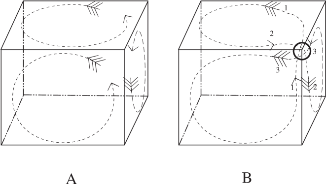
Figure 2: Changing orientation on the cube

In section 3 we obtain an upper and lower bound on the number of faces given in theorem 1.2. The lower bound is obtained by counting the number of faces that are simple closed paths on the graph.

The upper bound on the number of faces is obtained by first dividing the faces into two groups:

a

Small faces $\hbox{\rm length}(\mathcal{F})\leq\sqrt{(}n)$

b

Large faces $\sqrt{n}\leq\hbox{\rm length}(\mathcal{F})$

The number of large faces is easily bounded: since the total number of edges is $\frac{3n}{2}$ and each edge has two sides, we obtain that $\#(\mathcal{F}_{\geq\sqrt{n}})\leq 3\sqrt{n}$.

To estimate the number of small faces we first introduce the notion of root.

Definition 2.1.

A root in $(\Gamma,{\mathcal{O}})$ is a simple closed path in $\Gamma$, such that the orientation ${\mathcal{O}}$ agrees with the root in all but maybe one vertex.

Lemma 2.1.

Each face contains at least one root:

Proof: Pick a vertex $v_{1}$ and start walking along a left hand path until the path intersects itself, i.e., $v_{i}=v_{j}$ $i\neq j$ is the first intersection, then the cycle $v_{i},\cdots v_{j}$ is a root (in all the vertices $v_{l}$ $i<l<j$ the orientation agrees with the cycle).

In section 3 we will prove that the expected number of roots of length less than $\sqrt{n}$, and therefore the total number of small faces, is bounded by $O(\sqrt{n})$. By adding the number of short and long faces we get that the total number of faces is $<O(\sqrt{n})$; from equation 1 we deduce our main result 1.1.

3 Computing the Expectation

This section is devoted to the proof of theorem 1.2. Let $G_{n,d}$ be the space of $d$-regular graphs with $n$ vertices. We shall, following Bollobas, represent our graphs as the images of so-called configurations. Let $W=\bigcup_{j=1}^{n}W_{j}$ be a fixed set of $2m=nd$ vertices, where $|W_{j}|=d$. A configuration $F$ is a partition of $W$ into $m$ pairs of vertices called edges of $F$. Clearly there are

$$N=N(m)=\binom{2m}{2}\binom{2m-2}{2}\dots\binom{2}{2}/m!=\frac{(2m)_{m}}{2^{m}}$$ (2)

configurations. (We write $(a)_{b}=a(a-1)\dots(a-b+1)$).

Let $\Phi$ be a set of configurations. We now define a map $\Phi\rightarrow G_{n,d}$ as follows. Given a configuration $F$ let $\phi(F)$ be the graph with vertex set $V={1,\dots,n}$ in which $ij$ is an edge iff $F$ has a pair with one end in $W_{i}$ and the other in $W_{j}$. Every $G\in G_{n,d}$ is the image of $G=\phi(F)$ for $(d!)^{n}$ configurations. The number of configurations containing a given fixed set of $l$ edges is

$$\begin{split}N_{l}(m)&=\binom{2m-2l}{2}\binom{2m-2l-2}{2}\dots\binom{2}{2}/(m-l)!\\ &=\frac{N(m)}{(2m-1)(2m-3)\dots(2m-2l+1)}\\ \end{split}$$ (3)

From (2) and (3), the probability that a configuration contains a given set of $l$ edges is

$$\begin{split}\frac{N(m-l)}{N(m)}&=\frac{1}{(2m-1)(2m-3)\dots(2m-2l+1)}\\ &=\frac{1}{2^{l}}\frac{\Gamma(m-l+\frac{1}{2})}{\Gamma(m+\frac{1}{2})}\\ \end{split}$$ (4)

where we use

$$1\cdot 3\cdot 5\cdot\dots(2n-1)=2^{n}\Gamma(n+\frac{1}{2})\cdot\frac{1}{\sqrt{\pi}}$$

For $k\in\bf{N}$ a k-cycle of a configuration is a set of $k$ edges, say ${e_{1},\dots,e_{k}}$ such that for some $k$ distinct groups $W_{j_{1}},\dots,W_{j_{k}}$ the edge $e_{i}$ joins $W_{j_{i}}$ to $W_{j_{i+1}}$, where $W_{j_{k+1}}\equiv W_{j_{1}}$. A 1-cycle is said to be a loop and a 2-cycle is a coupling. Given a configuration $F$, denote by $X_{k}(F)$ the number of k-cycles. If we are to restrict to graphs in $G_{n,d}$ to have no loops and no multiple edges, then not every $\phi(F)$ belongs to $G_{n,d}$ but only those satisfying $X_{1}(F)=X_{2}(F)=0$; such graphs are called simple. (In order to restrict to graphs with $X_{1}=X_{2}=0$ we have to multiply all the ensuing estimates by $\bf{P}(\rm{simple})\sim\exp(\frac{1-d^{2}}{4})$.)

Let $C_{k}$ be the number of sets of pairs of vertices in $V$ which can be k-cycles of configurations. By elementary counting:

$$\ C_{k}=\frac{1}{2k}\frac{n!}{(n-k)!}(d(d-1))^{k}$$ (5)

Using (4) and (5) we get the following expression for the expected number of $k$-cycles:

$$\boldsymbol{E}(X_{k})=\frac{1}{2k}\frac{n!}{(n-k)!}(d(d-1))^{k}\frac{1}{2^{k}}\frac{\Gamma(m-k+\frac{1}{2})}{\Gamma(m+\frac{1}{2})}$$ (6)

To obtain a lower bound on the number of faces $\mathcal{F}$, we count the number of faces that are simple closed paths. For each simple closed path of length $k$ the probability of correct orientation is $\frac{1}{(d-1)^{k}}$, consequently we have:

$$\boldsymbol{E}(\mathcal{F})>\sum_{3}^{m}\frac{\boldsymbol{E}(X_{k})}{(d-1)^{k}}=\sum_{3}^{m}\frac{a_{k}}{k},$$ (7)

where

$$a_{k}=\frac{d^{k}}{2^{k}}\frac{n!}{(n-k)!}\frac{\Gamma(m-k+\frac{1}{2})}{\Gamma(m+\frac{1}{2})}.$$ (8)

Now using Stirling’s formula (with $x$ positive real),

$$\Gamma(x)=\sqrt{2\pi}x^{x-\frac{1}{2}}e^{-x}\left(1+O\left(\frac{1}{x}\right)\right),$$

we have for $k=o(n^{2/3})$

$$\frac{n!}{(n-k)!}=n^{k}e^{\frac{k^{2}}{2n}}\left(1+O\left(\frac{k}{n}\right)+O\left(\frac{k^{3}}{n^{2}}\right)\right);$$

and similarly

$$\frac{\Gamma(m-k+\frac{1}{2})}{\Gamma(m+\frac{1}{2})}=m^{-k}e^{\frac{k^{2}}{2m}}\left(1+O\left(\frac{k}{n}\right)\right).$$

Recalling that $m=\frac{nd}{2}$, we have

$$a_{k}=e^{-\frac{(d-2)k^{2}}{2nd}}\left(1+O\left(\frac{k}{n}\right)\right).$$ (9)

The estimate (9) and the fact that $a_{k}$ are monotonic decreasing in $k$, show that if we let $k$ range from $3$ to $m^{t}$ where $t>1/2$, the remaining terms in (7) are negligible. With that in mind, let $b$ be an arbitrary positive number independent of $m$. If $k^{2}\leq bm$, the estimate in (9) is between $1$ and $\exp{(-b/2)}$. Using

$$1+\frac{1}{2}+\dots+\frac{1}{l}\sim\log{l}$$

we get that the asymptotic estimate for that part of sum in (7) with $3\leq k\leq\sqrt{bm}$ is between $(\log m)/2$ and $e^{-b/2}(\log m)/2$. For the remainder of the sum, $\frac{1}{k}<\sqrt{bm}$, and the sum of $\exp(-k^{2}/2m)$ is asymptotic to $\sqrt{m}$ times an integral of $\exp(-x^{2}/2)$. It follows that for any value of $b$, the contribution of this part of sum is bounded as $m\to\infty$, and so (7) is asymptotic to a function of $m$ which lies between $(\log m)/2$ and $\exp(-b/2)(\log m)/2$. Since $b$ is arbitrary, $\exp(-b/2)$ can be made as close to 1 as desired; hence we obtain that the sum in (7) is asymptotic to $(\log m)/2$.

Now we turn to estimating the number of faces from above. Recall that the number of large faces is bounded from above by $\sqrt{m}$, so we need to estimate from above the number of small faces. As their length is less than $\sqrt{m}$, so is the length of their roots; thus the estimate on the number of roots of length less than $\sqrt{m}$ will suffice.

Now given a cycle of length $k$, we can turn it into a root in $(k+1)$ ways: one simple face and $k$ proper roots. Furthermore, the probability of correct orientation is $\frac{1}{(d-1)^{k}}$. So we have the following estimate (with $a_{k}$ given in 8):

$$\boldsymbol{E}(\mathcal{F}_{\leq\sqrt{m}})<\sum_{k=3}^{\sqrt{m}}\frac{k+1}{(d-1)^{k}}\boldsymbol{E}(X_{k})=\frac{1}{2}\sum_{k=3}^{\sqrt{m}}a_{k}+\frac{1}{2}\sum_{k=3}^{\sqrt{m}}\frac{a_{k}}{k}.$$

The second sum is clearly dominated by the sum in (7), which we established to be of order $O(\log{m})$. For the first sum, using (9), we obtain

$$\sum_{k=3}^{\sqrt{m}}a_{k}=\sum_{k=3}^{\sqrt{m}}e^{-\frac{(d-2)k^{2}}{2nd}}\left(1+O\left(\frac{k}{n}\right)\right)<\sqrt{nd}\int_{0}^{\infty}e^{-\frac{x^{2}}{2}}\mathrm{d}x+O(1)=O(\sqrt{n})$$

We have therefore established upper and lower bound of $O(\sqrt{n})$ and $O(\log{n})$ respectively for the number of faces, proving the theorem 1.2.

References

- [Bel] G. V. Belyi, Galois extensions of a maximal cyclotomic field, Izv. Akad. Nauk SSSR Ser. Mat. 43, 1979, 267-276.
- [Bol1] Béla Bollobás, Random graphs, Academic Press Inc. [Harcourt Brace Jovanovich Publishers], London, 1985.
- [Bol2] , The isoperimetric number of random regular graphs, European J. Combin. 9 (1988), no. 3, 241–244.
- [BM] Robert Brooks and Eran Makover, Random Construction of Riemann Surfaces preprint.
- [SH] Saul Stahl, On the average genus of the random graph, J. Graph Theory 20 (1995), no. 1, 1–18.