On the Minimum Ropelength of Knots and Links

Abstract

The ropelength of a knot is the quotient of its length by its thickness, the radius of the largest embedded normal tube around the knot. We prove existence and regularity for ropelength minimizers in any knot or link type; these are $C^{1,1}$ curves, but need not be smoother. We improve the lower bound for the ropelength of a nontrivial knot, and establish new ropelength bounds for small knots and links, including some which are sharp.

Introduction

How much rope does it take to tie a knot? We measure the ropelength of a knot as the quotient of its length and its thickness, the radius of the largest embedded normal tube around the knot. A ropelength-minimizing configuration of a given knot type is called tight.

Tight configurations make interesting choices for canonical representatives of each knot type, and are also referred to as “ideal knots”. It seems that geometric properties of tight knots and links are correlated well with various physical properties of knotted polymers. These ideas have attracted special attention in biophysics, where they are applied to knotted loops of DNA. Such knotted loops are important tools for studying the behavior of various enzymes known as topoisomerases. For information on these applications, see for instance [Sum, SKB⁺, KBM⁺, KOP⁺, DS1, DS2, CKS, LKS⁺] and the many contributions to the book Ideal Knots [SKK].

In the first section of this paper, we show the equivalence of various definitions that have previously been given for thickness. We use this to demonstrate that in any knot or link type there is a ropelength minimizer, and that minimizers are necessarily $C^{1,1}$ curves (Theorem 2.9).

The main results of the paper are several new lower bounds for ropelength, proved by considering intersections of the normal tube and a spanning surface. For a link of unit thickness, if one component is linked to $n$ others, then its length is at least $2\pi+P_{n}$, where $P_{n}$ is the length of the shortest curve surrounding $n$ disjoint unit-radius disks in the plane (Theorem 3.5). This bound is sharp in many simple cases, allowing us to construct infinite families of tight links, such as the simple chain shown in Figure 1. The only previously known example of a tight link was the Hopf link built from two round circles, which was the solution to the Gehring link problem [ES, Oss, Gag]. Our new examples show that ropelength minimizers need not be $C^{2}$, and need not be unique.

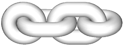
Figure 1: A simple chain of $k\geq 2$ rings, the connect sum of $k-1$ Hopf links, can be built from stadium curves (with circles at the ends). This configuration has ropelength $(4\pi+4)k-8$ and is tight by Theorem 3.5; it shows that ropelength minimizers need not be $C^{2}$.

Next, if one component in a unit-thickness link has total linking number $n$ with the other components, then its length is at least $2\pi+2\pi\sqrt{n}$, by Theorem 4.1. We believe that this bound is never sharp for $n>1$. We obtain it by using a calibration argument to estimate the area of a cone surface spanning the given component, and the isoperimetric inequality to convert this to a length bound. For links with linking number zero, we need a different approach: here we get better ropelength bounds (Theorem 8.2) in terms of the asymptotic crossing number of Freedman and He [FH].

Unit-thickness knots have similar lower bounds on length, but the estimates are more intricate and rely on two additional ideas. In Theorem 6.7, we prove the existence of a point from which any nontrivial knot has cone angle at least $4\pi$. In Section 5, we introduce the parallel overcrossing number of a knot, which measures how many times it crosses over a parallel knot: we conjecture that this equals the crossing number, and we prove it is at least the bridge number (Proposition 5.4). Combining these ideas, we show (Theorem 7.1) that any nontrivial knot has ropelength at least $4\pi+2\pi\sqrt{2}\approx 6.83\pi\approx 21.45$. The best previously known lower bound [LSDR] was $5\pi\approx 15.71$. Computer experiments [SDKP] using Pieranski’s SONO algorithm [Pie] suggest that the tight trefoil has ropelength around $32.66$. Our improved estimate still leaves open the old question of whether any knot has ropelength under $24$, that is: Can a knot be tied in one foot of one-inch (diameter) rope?

1 Definitions of Thickness

To define the thickness of a curve, we follow the paper [GM] of Gonzalez and Maddocks. Although they considered only smooth curves, their definition (unlike most earlier ones, but see [KS]) extends naturally to the more general curves we will need. In fact, it is based on Menger’s notion (see [BM, §10.1]) of the three-point curvature of an arbitrary metric space.

For any three distinct points $x$, $y$, $z$ in ${\mathbb{R}}^{3}$, we let $r(x,y,z)$ be the radius of the (unique) circle through these points (setting $r=\infty$ if the points are collinear). Also, if $V_{x}$ is a line through $x$, we let $r(V_{x},y)$ be the radius of the circle through $y$ tangent to $V_{x}$ at $x$.

Now let $L$ be a link in ${\mathbb{R}}^{3}$, that is, a disjoint union of simple closed curves. For any $x\in L$, we define the thickness $\tau(L)$ of $L$ in terms of a local thickness $\tau_{x}(L)$ at $x\in L$:

$$\tau(L):=\inf_{x\in L}\tau_{x}(L),\qquad\tau_{x}(L):=\mskip-3.0mu\mskip-3.0mu\inf_{\begin{subarray}{c}y,z\in L\\ x\neq y\neq z\neq x\end{subarray}}\mskip-3.0mu\mskip-3.0mur(x,y,z).$$

To apply this definition to nonembedded curves, note that we consider only triples of distinct points $x,y,z\in{\mathbb{R}}^{3}$. We will see later that a nonembedded curve must have zero thickness unless its image is an embedded curve, possibly covered multiple times.

Note that any sphere cut three times by $L$ must have radius greater than $\tau(L)$. This implies that the closest distance between any two components of $L$ is at least $2\tau$, as follows: Consider a sphere whose diameter achieves this minimum distance; a slightly larger sphere is cut four times.

We usually prefer not to deal explicitly with our space curves as maps from the circle. But it is important to note that below, when we talk about curves being in class $C^{k,\alpha}$, or converging in $C^{k}$ to some limit, we mean with respect to the constant-speed parametrization on the unit circle.

Our first two lemmas give equivalent definitions of thickness. The first shows that the infimum in the definition of $\tau(L)$ is always attained in a limit when (at least) two of the three points approach each other. Thus, our definition agrees with one given earlier by Litherland et al. [LSDR] for smooth curves. If $x\neq y\in L$ and $x-y$ is perpendicular to both $T_{x}L$ and $T_{y}L$, then we call $|x-y|$ a doubly critical self-distance for $L$.

Lemma 1.1.

Suppose $L$ is $C^{1}$, and let $T_{x}L$ be its tangent line at $x\in L$. Then the thickness is given by

$$\tau(L)=\mskip-3.0mu\inf_{x\neq y\in L}r(T_{x}L,y).$$

This equals the infimal radius of curvature of $L$ or half the infimal doubly critical self-distance, whichever is less.

Proof 1.2.

The infimum in the definition of thickness either is achieved for some distinct points $x$, $y$, $z$, or is approached along the diagonal when $z$, say, approaches $x$, giving us $r(T_{x}L,y)$. But the first case cannot happen unless the second does as well: consider the sphere of radius $\tau=r(x,y,z)$ with $x$, $y$ and $z$ on its equator, and relabel the points if necessary so that $y$ and $z$ are not antipodal. Since this $r$ is infimal, $L$ must be tangent to the sphere at $x$. Thus $r(T_{x}L,y)\leq\tau$, and we see that $\tau(L)=\inf r(T_{x}L,y)$. This infimum, in turn, is achieved either for some $x\neq y$, or in a limit as $y\to x$ (when it is the infimal radius of curvature). In the first case, we can check that $x$ and $y$ must be antipodal points on a sphere of radius $\tau$, with $L$ tangent to the sphere at both points. That means, by definition, that $2\tau$ is a doubly critical self-distance for $L$. ∎

A version of Lemma 1.1 for smooth curves appeared in [GM]. Similar arguments there show that the local thickness can be computed as

$$\tau_{x}(L)=\inf_{y\neq x}r(T_{y}L,x).$$

Lemma 1.3.

For any $C^{1}$ link $L$, the thickness of $L$ equals the reach of $L$; this is also the normal injectivity radius of $L$.

The reach of a set $L$ in ${\mathbb{R}}^{3}$, as defined by Federer [Fed], is the largest $\rho$ for which any point $p$ in the $\rho$-neighborhood of $L$ has a unique nearest point in $L$. The normal injectivity radius of a $C^{1}$ link $L$ in ${\mathbb{R}}^{3}$ is the largest $\iota$ for which the union of the open normal disks to $L$ of radius $\iota$ forms an embedded tube.

Proof 1.4.

Let $\tau$, $\rho$, and $\iota$ be the thickness, reach, and normal injectivity radius of $L$. We will show that $\tau\leq\rho\leq\iota\leq\tau$.

Suppose some point $p$ has two nearest neighbors $x$ and $y$ at distance $\rho$. Thus $L$ is tangent at $x$ and $y$ to the sphere around $p$, so a nearby sphere cuts $L$ four times, giving $\tau\leq\rho$.

Similarly, suppose some $p$ is on two normal circles of $L$ of radius $\iota$. This $p$ has two neighbors on $L$ at distance $\iota$, so $\rho\leq\iota$.

We know that $\iota$ is less than the infimal radius of curvature of $L$. Furthermore, the midpoint of a chord of $L$ realizing the infimal doubly self-critical distance of $L$ is on two normal disks of $L$. Using Lemma 1.1, this shows that $\iota\leq\tau$, completing the proof. ∎

If $L$ has thickness $\tau>0$, we will call the embedded (open) normal tube of radius $\tau$ around $L$ the thick tube around $L$.

We define the ropelength of a link $L$ to be $\operatorname{Len}(L)/\tau(L)$, the (scale-invariant) quotient of length over thickness. Every curve of finite roplength is $C^{1,1}$, by Lemma 2.3 below. Thus, we are free to restrict our attention to $C^{1,1}$ curves, rescaled to have (at least) unit thickness. This means they have embedded unit-radius normal tubes, and curvature bounded above by $1$. The ropelength of such a curve is (at most) its length.

2 Existence and Regularity of Ropelength Minimizers

We want to prove that, within every knot or link type, there exist curves of minimum ropelength. The lemma below allows us to use the direct method to get minimizers. If we wanted to, we could work with $C^{1}$ convergence in the space of $C^{1,1}$ curves, but it seems better to state the lemma in this stronger form, applying to all rectifiable links.

Lemma 2.1.

Thickness is upper semicontinuous with respect to the $C^{0}$ topology on the space of $C^{0,1}$ curves.

Proof 2.2.

This follows immediately from the definition, since $r(x,y,z)$ is a continuous function (from the set of triples of distinct points in space) to $(0,\infty]$. For, if curves $L_{i}$ approach $L$, and $r(x,y,z)$ nearly realizes the thickness of $L$, then nearby triples of distinct points bound from above the thicknesses of the $L_{i}$. ∎

This proof (compare [KS]) is essentially the same as the standard one for the lower semicontinuity of length, when length of an arbitrary curve is defined as the supremal length of inscribed polygons. Note that thickness can jump upwards in a limit, even when the convergence is $C^{1}$. For instance, we might have an elbow consisting of two straight segments connected by a unit-radius circular arc whose angle decreases to zero, as shown in Figure 2.

Figure 2: These elbow curves consist of straight segments connected by a circular arc of unit radius. No matter how small the angle of the arc is, the curve has unit thickness, as demonstrated by the maximal embedded normal neighborhoods shown. These $C^{1,1}$ curves converge in $C^{1}$ to a straight segment, with infinite thickness.

When minimizing ropelength within a link type, we care only about links of positive thickness $\tau>0$. We next prove three lemmas about such links. It will be useful to consider the secant map $S$ for a link $L$, defined, for $x\neq y\in L$, by

$$S(x,y):=\pm\frac{x-y}{|x-y|}\in{\mathbb{R}}P^{2}.$$

Note that as $x\to y$, the limit of $S(x,y)$, if it exists, is the tangent line $T_{y}L$. Therefore, the link is $C^{1}$ exactly if $S$ extends continuously to the diagonal $\Delta$ in $L\times L$, and is $C^{1,1}$ exactly when this extension is Lipschitz. When speaking of particular Lipschitz constants we use the following metrics: on $L\times L$, we sum the (shorter) arclength distances in the factors; on ${\mathbb{R}}P^{2}$ the distance between two points is $d=\sin\theta$, where $\theta$ is the angle between (any) lifts of the points to ${\mathbb{S}}^{2}$.

Lemma 2.3.

If $L$ has thickness $\tau>0$, then its secant map $S$ has Lipschitz constant $1/2\tau$. Thus $L$ is $C^{1,1}$.

Proof 2.4.

We must prove that $S$ has Lipschitz constant $1/2\tau$ on $(L\times L)\smallsetminus\Delta$; it then has a Lipschitz extension. By the triangle inequality, it suffices to prove, for any fixed $x\in L$, that $d\big{(}S(x,y),S(x,z)\big{)}\leq|y-z|/2\tau$ whenever $y$ and $z$ are sufficiently close along $L$. Setting $\theta:=\angle zxy$, we have

$$d\big{(}S(x,y),S(x,z)\big{)}=\sin\theta=\frac{|y-z|}{2\,r(x,y,z)}\leq\frac{|y-z|}{2\tau},$$

using the law of sines and the definition $\tau:=\inf r$. ∎

Figure 3: The secant map for a thick knot is Lipschitz by Lemma 2.3: when $y$ and $z$ are close along the knot, the secant directions $\overline{xy}$ and $\overline{xz}$ are close. Here $r=r(x,y,z)$ is an upper bound for the thickness of the knot.

Although we are primarily interested in links (embedded curves), we note that Lemma 2.3 also shows that a nonembedded curve $L$ must have thickness zero, unless its image is contained in some embedded curve. For such a curve $L$ contains some point $p$ where at least three arcs meet, and at least one pair of those arcs will fail to join in a $C^{1,1}$ fashion at $p$.

Lemma 2.5.

If $L$ is a link of thickness $\tau>0$, then any points $x,y\in L$ with $|x-y|<2\tau$ are connected by an arc of $L$ of length at most

$$2\tau\arcsin\frac{|x-y|}{2\tau}\,\leq\,\frac{\pi}{2}\,|x-y|.$$

Proof 2.6.

The two points $x$ and $y$ must be on the same component of $L$, and one of the arcs of $L$ connecting them is contained in the ball with diameter $\overline{xy}$. By Lemma 1.1, the curvature of $L$ is less than $1/\tau$. Thus by Schur’s lemma, the length of this arc of $L$ is at most $2\tau\arcsin(|x-y|/2\tau)$, as claimed. Note that Chern’s proof [Che] of Schur’s lemma for space curves, while stated only for $C^{2}$ curves, applies directly to $C^{1,1}$ curves, which have Lipschitz tantrices on the unit sphere. (As Chern notes, the lemma actually applies even to curves with corners, when correctly interpreted.) ∎

Lemma 2.7.

Suppose $L_{i}$ is a sequence of links of thickness at least $\tau>0$, converging in $C^{0}$ to a limit link $L$. Then the convergence is actually $C^{1}$, and $L$ is isotopic to (all but finitely many of) the $L_{i}$.

Proof 2.8.

To show $C^{1}$ convergence, we will show that the secant maps of the $L_{i}$ converge (in $C^{0}$) to the secant map of $L$. Note that when we talk about convergence of the secant maps, we view them (in terms of constant-speed parametrizations of the $L_{i}$) as maps from a common domain. Since these maps are uniformly Lipschitz, it suffices to prove pointwise convergence.

So consider a pair of points $p$, $q$ in $L$. Take $\epsilon<|p-q|$. For large enough $i$, $L_{i}$ is within $\epsilon^{2}/2$ of $L$ in $C^{0}$, and hence the corresponding points $p_{i}$, $q_{i}$ in $L_{i}$ have $|p_{i}-p|<\epsilon^{2}/2$ and $|q_{i}-q|<\epsilon^{2}/2$. We have moved the endpoints of the segment $\overline{pq}$ by relatively small amounts, and expect its direction to change very little. In fact, the angle $\theta$ between $p_{i}-q_{i}$ and $p-q$ satisfies $\sin\theta<(\epsilon^{2}/2+\epsilon^{2}/2)/\epsilon=\epsilon$. That is, the distance in ${\mathbb{R}}P^{2}$ between the points $S_{i}(p_{i},q_{i})$ and $S(p,q)$ is given by $\sin\theta<\epsilon$.

Therefore, the secant maps converge pointwise, which shows that the $L_{i}$ converge in $C^{1}$ to $L$. Since the limit link $L$ has thickness at least $\tau$ by Lemma 2.1, it is surrounded by an embedded normal tube of diameter $\tau$. Furthermore, all (but finitely many) of the $L_{i}$ lie within this tube, and by $C^{1}$ convergence are transverse to each normal disk. Each such $L_{i}$ is isotopic to $L$ by a straight-line homotopy within each normal disk. ∎

Our first theorem establishes the existence of tight configurations (ropelength minimizers) for any link type. This problem is interesting only for tame links: a wild link has no $C^{1,1}$ realization, so its ropelength is always infinite.

Theorem 2.9.

There is a ropelength minimizer in any (tame) link type; any minimizer is $C^{1,1}$, with bounded curvature.

Proof 2.10.

Consider the compact space of all $C^{1,1}$ curves of length at most $1$. Among those isotopic to a given link $L_{0}$, find a sequence $L_{i}$ supremizing the thickness. The lengths of $L_{i}$ approach $1$, since otherwise rescaling would give thicker curves. Also, the thicknesses approach some $\tau>0$, the reciprocal of the infimal ropelength for the link type. Replace the sequence by a subsequence converging in the $C^{1}$ norm to some link $L$. Because length is lower semicontinuous, and thickness is upper semicontinuous (by Lemma 2.1), the ropelength of $L$ is at most $1/\tau$. By Lemma 2.7, all but finitely many of the $L_{i}$ are isotopic to $L$, so $L$ is isotopic to $L_{0}$.

By Lemma 2.3, tight links must be $C^{1,1}$, since they have positive thickness. ∎

This theorem has been extended by Gonzalez et al. [GM+], who minimize a broad class of energy functionals subject to the constraint of fixed thickness. See also [GdlL].

Below, we will give some examples of tight links which show that $C^{2}$ regularity cannot be expected in general, and that minimizers need not be unique.

3 The Ropelength of Links

Suppose in a link $L$ of unit thickness, some component $K$ is topologically linked to $n$ other components $K_{i}$. We will give a sharp lower bound on the length of $K$ in terms of $n$. When every component is linked to $n\leq 5$ others, this sharp bound lets us construct tight links.

To motivate the discussion below, suppose $K$ was a planar curve, bounding some region $R$ in the plane. Each $K_{i}$ would then have to puncture $R$. Since each $K_{i}$ is surrounded by a unit-radius tube, these punctures would be surrounded by disjoint disks of unit radius, and these disks would have to avoid a unit-width ribbon around $K$. It would then be easy to show that the length of $K$ was at least $2\pi$ more than $P_{n}$, the length of the shortest curve surrounding $n$ disjoint unit-radius disks in the plane.

To extend these ideas to nonplanar curves, we need to consider cones. Given a space curve $K$ and a point $p\in{\mathbb{R}}^{3}$, the cone over $K$ from $p$ is the disk consisting of all line segments from $p$ to points in $K$. The cone is intrinsically flat away from the single cone point $p$, and the cone angle is defined to be the angle obtained at $p$ if we cut the cone along any one segment and develop it into the Euclidean plane. Equivalently, the cone angle is the length of the projection of $K$ to the unit sphere around $p$. Note that the total Gauss curvature of the cone surface equals $2\pi$ minus this cone angle.

Our key observation is that every space curve may be coned to some point $p$ in such a way that the intrinsic geometry of the cone surface is Euclidean. We can then apply the argument above in the intrinsic geometry of the cone. In fact, we can get even better results when the cone angle is greater than $2\pi$. We first prove a technical lemma needed for this improvement. Note that the lemma would remain true without the assumptions that $K$ is $C^{1,1}$ and has curvature at most $1$. But we make use only of this case, and the more general case would require a somewhat more complicated proof.

Lemma 3.1.

Let $S$ be an infinite cone surface with cone angle $\theta\geq 2\pi$ (so that $S$ has nonpositive curvature and is intrinsically Euclidean away from the single cone point). Let $R$ be a subset of $S$ which includes the cone point, and let $\ell$ be a lower bound for the length of any curve in $S$ surrounding $R$. Consider a $C^{1,1}$ curve $K$ in $S$ with geodesic curvature bounded above by $1$. If $K$ surrounds $R$ while remaining at least unit distance from $R$, then $K$ has length at least $\ell+\theta$.

Proof 3.2.

We may assume that $K$ has nonnegative geodesic curvature almost everywhere. If not, we simply replace it by the boundary of its convex hull within $S$, which is well-defined since $S$ has nonpositive curvature. This boundary still surrounds $R$ at unit distance, is $C^{1,1}$, and has nonnegative geodesic curvature.

For $t<1$, let $K_{t}$ denote the inward normal pushoff, or parallel curve to $K$, at distance $t$ within the cone. Since the geodesic curvature of $K$ is bounded by $1$, these are all smooth curves, surrounding $R$ and hence surrounding the cone point. If $\kappa_{g}$ denotes the geodesic curvature of $K_{t}$ in $S$, the formula for first variation of length is

$$\frac{d}{dt}\operatorname{Len}(K_{t})=-\int_{\mskip-3.0muK_{t}}\mskip-3.0mu\mskip-3.0mu\kappa_{g}\,\operatorname{ds}=-\theta,$$

where the last equality comes from Gauss–Bonnet, since $S$ is intrinsically flat except at the cone point. Thus $\operatorname{Len}(K)=\operatorname{Len}(K_{t})+t\theta$; since $K_{t}$ surrounds $R$ for every $t<1$, it has length at least $\ell$, and we conclude that $\operatorname{Len}(K)\geq\ell+\theta$. ∎

Lemma 3.3.

For any closed curve $K$, there is a point $p$ such that the cone over $K$ from $p$ has cone angle $2\pi$. When $K$ has positive thickness, we can choose $p$ to lie outside the thick tube around $K$.

Proof 3.4.

Recall that the cone angle at $q$ is given by the length of the radial projection of $K$ onto the unit sphere centered at $q$. If we choose $q$ on a chord of $K$, this projection joins two antipodal points, and thus must have length at least $2\pi$. On any doubly critical chord (for instance, the longest chord) the point $q$ at distance $\tau(K)$ from either endpoint must lie outside the thick tube, by Lemma 1.3.

Note that the cone angle approaches $0$ at points far from $K$. The cone angle is a continuous function on the complement of $K$ in ${\mathbb{R}}^{3}$, a connected set. When $K$ has positive thickness, even the complement of its thick tube is connected. Thus if the cone angle at $q$ is greater than $2\pi$, the intermediate value theorem lets us choose some $p$ (outside the tube) from which the cone angle is exactly $2\pi$. Figure 4 shows such a cone on a trefoil knot. ∎

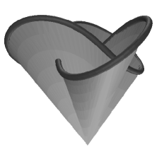
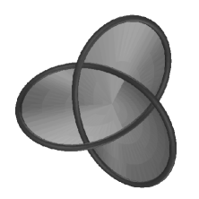
Figure 4: Two views of the same cone, whose cone angle is precisely $2\pi$, on a symmetric trefoil knot.

Our first ropelength bound will be in terms of a quantity we call $P_{n}$, defined to equal the shortest length of any plane curve enclosing $n$ disjoint unit disks. Considering the centers of the disks, using Lemma 3.1, and scaling by a factor of $2$, we see that $P_{n}=2\pi+2Q_{n}$, where $Q_{n}$ is the length of the shortest curve enclosing $n$ points separated by unit distance in the plane.

For small $n$ it is not hard to determine $Q_{n}$ and $P_{n}$ explicitly from the minimizing configurations shown in Figure 5. Clearly $P_{1}=2\pi$, while for $2\leq n\leq 5$, we have $P_{n}=2\pi+2n$ since $Q_{n}=n$. Note that the least-perimeter curves in Figure 5 are unique for $n<4$, but for $n=4$ there is a continuous family of minimizers. For $n=5$ there is a two-parameter family, while for $n=6$ the perimeter-minimizer is again unique, with $Q_{6}=4+\sqrt{3}$. It is clear that $Q_{n}$ grows like $\sqrt{n}$ for $n$ large.

$n$	$1$	$2$	$3$
$P_{n}$	$2\pi$	$2\pi+4$	$2\pi+6$

$n$	$4$
$P_{n}$	$2\pi+8$

Figure 5: The shortest curve enclosing $n$ unit disks in the plane has length $P_{n}$, and is unique for $n<4$. For $n=4$, there is a one-parameter family of equally short curves.

Theorem 3.5.

Suppose $K$ is one component of a link of unit thickness, and the other components can be partitioned into $n$ sublinks, each of which is topologically linked to $K$. Then the length of $K$ is at least $2\pi+P_{n}$, where $P_{n}$ is the minimum length of any curve surrounding $n$ disjoint unit disks in the plane.

Proof 3.6.

By Lemma 3.3 we can find a point $p$ in space, outside the unit-radius tube surrounding $K$, so that coning $K$ to $p$ gives a cone of cone angle $2\pi$, which is intrinsically flat.

Each of the sublinks $L_{i}$ nontrivially linked to $K$ must puncture this spanning cone in some point $p_{i}$. Furthermore, the fact that the link has unit thickness implies that the $p_{i}$ are separated from each other and from $K$ by distance at least $2$ in space, and thus by distance at least $2$ within the cone.

Thus in the intrinsic geometry of the cone, the $p_{i}$ are surrounded by disjoint unit-radius disks, and $K$ surrounds these disks while remaining at least unit distance from them. Since $K$ has unit thickness, it is $C^{1,1}$ with curvature bounded above by $1$. Since the geodesic curvature of $K$ on the cone surface is bounded above by the curvature of $K$ in space, we can apply Lemma 3.1 to complete the proof. ∎

For $n\leq 5$, it is easy to construct links which achieve these lower bounds and thus must be tight. We just ensure that each component linking $n$ others is a planar curve of length equal to our lower bound $2\pi+P_{n}$. In particular, it must be the outer boundary of the unit neighborhood of some curve achieving $P_{n}$. In this way we construct the tight chain of Figure 1, as well as infinite families of more complicated configurations, including the link in Figure 6. These examples may help to calibrate the various numerical methods that have been used to compute ropelength minimizers [Pie, Raw, Lau]. For $n\geq 6$, this construction does not work, as we are unable to simultaneously minimize the length of $K$ and the length of all the components it links.

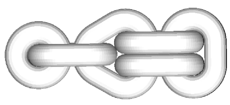
Figure 6: Each component in this link uses one of the perimeter-minimizing shapes from Figure 5, according to how many other components it links. The link is therefore tight by Theorem 3.5. This minimizer is not unique, in that some components could be rotated relative to others. In other examples, even the shape of individual components (linking four others) fails to be unique.

These explicit examples of tight links answer some existing questions about ropelength minimizers. First, these minimizers fail, in a strong sense, to be unique: there is a one-parameter family of tight five-component links based on the family of curves with length $P_{4}$. So we cannot hope to add uniqueness to the conclusions of Theorem 2.9. In addition, these minimizers (except for the Hopf link) are not $C^{2}$. This tells us that there can be no better global regularity result than that of Theorem 2.9. However, we could still hope that every tight link is piecewise smooth, or even piecewise analytic.

Finally, note that the ropelength of a composite link should be somewhat less than the sum of the lengths of its factors. It was observed in [SKB⁺] that this deficit seems to be at least $4\pi-4$. Many of our provably tight examples, like the simple chain in Figure 1 or the link in Figure 6, are connect sums which give precise confirmation of this observation.

4 Linking Number Bounds

We now adapt the cone surface arguments to find a lower bound on ropelength in terms of the linking number. These bounds are more sensitive to the topology of the link, but are not sharp, and thus provide less geometric information. In Section 8, we will present a more sophisticated argument, which implies Theorem 4.1 as a consequence. However, the argument here is concrete enough that it provides a nice introduction to the methods used in the rest of the paper.

Theorem 4.1.

Suppose $L$ is a link of unit thickness. If $K$ is one component of the link, and $J$ is the union of any collection of other components, let $\operatorname{Lk}(J,K)$ denote the total linking number of $J$ and $K$, for some choice of orientations. Then

$$\operatorname{Len}(K)\geq 2\pi+2\pi\sqrt{\operatorname{Lk}(J,K)}.$$

Proof 4.2.

As in the proof of Theorem 3.5, we apply Lemma 3.3 to show that we can find an intrinsically flat cone surface $S$ bounded by $K$. We know that $K$ is surrounded by an embedded unit-radius tube $T$; let $R=S\smallsetminus T$ be the portion of the cone surface outside the tube. Each component of $J$ is also surrounded by an embedded unit-radius tube disjoint from $T$. Let $V$ be the $C^{1}$ unit vectorfield normal to the normal disks of these tubes. A simple computation shows that $V$ is a divergence-free field, tangent to the boundary of each tube, with flux $\pi$ over each spanning surface inside each tube. A cohomology computation (compare [Can]) shows that the total flux of $V$ through $R$ is $\operatorname{Flux}_{R}(V)=\pi\operatorname{Lk}(J,K)$. Since $V$ is a unit vectorfield, this implies that

$$\operatorname{Flux}_{R}(V)=\int_{R}V\cdot\vec{n}\,\operatorname{dA}\leq\int_{R}\mskip-3.0mu\,\operatorname{dA}=\operatorname{Area}(R).$$

Thus $\operatorname{Area}(R)\geq\pi\operatorname{Lk}(J,K)$. The isoperimetric inequality within $S$ implies that any curve on $S$ surrounding $R$ has length at least $2\pi\sqrt{\operatorname{Lk}(J,K)}$. Since $L$ has unit thickness, the hypotheses of Lemma 3.1 are fulfilled, and we conclude that

$$\operatorname{Len}(K)\geq 2\pi+2\pi\sqrt{\operatorname{Lk}(J,K)},$$

completing the proof. ∎

Note that the term $2\pi\sqrt{\operatorname{Lk}(J,K)}$ is the perimeter of the disk with the same area as $n:=\operatorname{Lk}(J,K)$ unit disks. We might hope to replace this term by $P_{n}$, but this seems difficult: although our assumptions imply that $J$ punctures the cone surface $n$ times, it is possible that there are many more punctures, and it is not clear how to show that an appropriate set of $n$ are surrounded by disjoint unit disks.

For a link of two components with linking number $2$, like the one in Figure 7, this bound provides an improvement on Theorem 3.5, raising the lower bound on the ropelength of each component to $2\pi+2\pi\sqrt{2}$, somewhat greater than $4\pi$.

                      

Figure 7: The two components of this $(2,4)$-torus link have linking number two, so by Theorem 4.1, the total ropelength is at least $4\pi(1+\sqrt{2})\approx 33.34$. Laurie et al. [LKS⁺] have computed a configuration with ropelength approximately $41.2$.

We note that a similar argument bounds the ropelength of any curve $K$ of unit thickness, in terms of its writhe. We again consider the flux of $V$ through a flat cone $S$. If we perturb $K$ slightly to have rational writhe (as below in the proof of Theorem 8.2) and use the result that “link equals twist plus writhe” [Căl1, Whi2], we find that this flux is at least $|\mskip-3.0mu\operatorname{Wr}(K)|$, so that

$$\operatorname{Len}(K)\geq 2\pi\sqrt{|\mskip-3.0mu\operatorname{Wr}(K)|}\,.$$

There is no guarantee that this flux occurs away from the boundary of the cone, however, so Lemma 3.1 does not apply. Unfortunately, this bound is weaker than the corresponding result of Buck and Simon [BS],

$$\operatorname{Len}(K)\geq 4\pi\sqrt{|\mskip-3.0mu\operatorname{Wr}(K)|}\,.$$

5 Overcrossing Number

In Section 4, we found bounds on the ropelength of links; to do so, we bounded the area of that portion of the cone surface outside the tube around a given component $K$ in terms of the flux of a certain vectorfield across that portion of the surface. This argument depended in an essential way on linking number being a signed intersection number.

For knots, we again want a lower bound for the area of that portion of the cone that is at least unit distance from the boundary. But this is more delicate and requires a more robust topological invariant. Here, our ideas have paralleled those of Freedman and He (see [FH, He]) in many important respects, and we adopt some of their terminology and notation below.

Let $L$ be an (oriented) link partitioned into two parts $A$ and $B$. The linking number $\operatorname{Lk}(A,B)$ is the sum of the signs of the crossings of $A$ over $B$; this is the same for any projection of any link isotopic to $L$. By contrast, the overcrossing number $\operatorname{Ov}(A,B)$ is the (unsigned) number of crossings of $A$ over $B$, minimized over all projections of links isotopic to $L$.

Lemma 5.1.

For any link partitioned into two parts $A$ and $B$, the quantities $\operatorname{Lk}(A,B)$ and $\operatorname{Ov}(A,B)$ are symmetric in $A$ and $B$, and we have

$$|\operatorname{Lk}(A,B)|\leq\operatorname{Ov}(A,B)\,;\qquad\operatorname{Lk}(A,B)\equiv\operatorname{Ov}(A,B)\pmod{2}\,.$$

Proof 5.2.

To prove the symmetry assertions, take any planar projection with $n$ crossings of $A$ over $B$. Turning the plane over, we get a projection with $n$ crossings of $B$ over $A$; the signs of the crossings are unchanged. The last two statements are immediate from the definitions in terms of signed and unsigned sums. ∎

Given a link $L$, we define its parallel overcrossing number $\operatorname{PC}(L)$ to be the minimum of $\operatorname{Ov}(L,L^{\prime})$ taken over all parallel copies $L^{\prime}$ of the link $L$. That means $L^{\prime}$ must be an isotopic link such that corresponding components of $L$ and $L^{\prime}$ cobound annuli, the entire collection of which is embedded in ${\mathbb{R}}^{3}$. This invariant may be compared to Freedman and He’s asymptotic crossing number $\operatorname{AC}(L)$ of $L$, defined by

$$\operatorname{AC}(L)=\inf_{pL,qL}\frac{\operatorname{Ov}(pL,qL)}{|pq|},$$

where the infimum is taken over all degree-$p$ satellites $pL$ and degree-$q$ satellites $qL$ of $L$. (This means that $pL$ lies in a solid torus around $J$ and represents $p$ times the generator of the first homology group of that torus.) Clearly,

$$\operatorname{AC}(L)\leq\operatorname{PC}(L)\leq\operatorname{Cr}(L),$$

where $\operatorname{Cr}(L)$ is the crossing number of $L$. It is conjectured that the asymptotic crossing number of $L$ is equal to the crossing number. This would imply our weaker conjecture:

Conjecture 5.3.

If $L$ is any knot or link, $\operatorname{PC}(L)=\operatorname{Cr}(L)$.

To see why this conjecture is reasonable, suppose $K$ is an alternating knot of crossing number $k$. It is known [TL, Thi], using the Jones polynomial, that the crossing number of $K\cup K^{\prime}$ is least $4k$ for any parallel $K^{\prime}$. It is tempting to assume that within these $4k$ crossings of the two-component link, we can find not only $k$ self-crossings of each knot $K$ and $K^{\prime}$, but also $k$ crossings of $K$ over $K^{\prime}$ and $k$ crossings of $K^{\prime}$ over $K$. Certainly this is the case in the standard picture of $K$ and a planar parallel $K^{\prime}$.

Freedman and He have shown [FH] that for any knot,

$$\operatorname{AC}(K)\geq 2\operatorname{genus}(K)-1,$$

and hence that we have $\operatorname{AC}(K)\geq 1$ if $K$ is nontrivial. For the parallel overcrossing number, our stronger hypotheses on the topology of $L$ and $L^{\prime}$ allow us to find a better estimate in terms of the reduced bridge number $\operatorname{Br}(L)$. This is the minimum number of local maxima of any height function (taken over all links isotopic to $L$) minus the number of unknotted split components in $L$.

Proposition 5.4.

For any link $L$, we have $\operatorname{PC}(L)\geq\operatorname{Br}(L)$. In particular, if $L$ is nontrivial, $\operatorname{PC}(L)\geq 2$.

Proof 5.5.

By the definition of parallel overcrossing number, we can isotope $L$ and its parallel $L^{\prime}$ so that, except for $\operatorname{PC}(L,L^{\prime})$ simple clasps, $L^{\prime}$ lies above, and $L$ lies below, a slab in ${\mathbb{R}}^{3}$. Next, we can use the embedded annuli which cobound corresponding components of $L$ and $L^{\prime}$ to isotope the part of $L$ below the slab to the lower boundary plane of the slab. This gives a presentation of $L$ with $\operatorname{PC}(L)$ bridges, as in Figure 8. ∎

Figure 8: We show three stages of the proof of Proposition 5.4: At the left, we show a projection of $L\cup L^{\prime}$ with $\operatorname{PC}(L)$ overcrossings. In the center, we lift $L^{\prime}$ until it and $L$ lie respectively above and below a slab, except for $\operatorname{PC}(L)$ simple clasps. At the right, we isotope $L$ to flatten the undercrossings onto the boundary of the slab and thus show that the clasps are the only bridges in $L$.

6 Finding a Point with Larger Cone Angle

The bounds in Theorems 3.5 and 4.1 depended on Lemma 3.3 to construct a cone with cone angle $\theta=2\pi$, and on Lemma 3.1 to increase the total ropelength by at least $\theta$. For single unknotted curves, this portion of our argument is sharp: a convex plane curve has maximum cone angle $2\pi$, at points in its convex hull.

However, for nontrivial knots and links, we can improve our results by finding points with greater cone angle. In fact, we show every nontrivial knot or link has a $4\pi$ cone point. The next lemma is due to Gromov [Gro, Thm. 8.2.A] and also appears as [EWW, Thm. 1.3]:

Lemma 6.1.

Suppose $L$ is a link, and $M$ is a (possibly disconnected) minimal surface spanning $L$. Then for any point $p\in{\mathbb{R}}^{3}$ through which $n$ sheets of $M$ pass, the cone angle of $L$ at $p$ is at least $2\pi n$.

Proof 6.2.

Let $S$ be the union of $M$ and the exterior cone on $L$ from $p$. Consider the area ratio $\operatorname{Area}(S\cap B_{r}(p))/(\pi r^{2})$, where $B_{r}(p)$ is the ball of radius $r$ around $p$ in ${\mathbb{R}}^{3}$. As $r\to 0$, the area ratio approaches $n$, the number of sheets of $M$ passing through $p$; as $r\to\infty$, the ratio approaches the density of the cone on $L$ from $p$, which is the cone angle divided by $2\pi$. White has shown that the monotonicity formula for minimal surfaces continues to hold for $S$ in this setting [Whi1]: the area ratio is an increasing function of $r$. Comparing the limit values at $r=0$ and $r=\infty$ we see that the cone angle from $p$ is at least $2\pi n$. ∎

As an immediate corollary, we obtain:

Corollary 6.3.

If $L$ is a nontrivial link, then there is some point $p$ from which $L$ has cone angle at least $4\pi$.

Proof 6.4.

By the solution to the classical Plateau problem, each component of $L$ bounds some minimal disk. Let $M$ be the union of these disks. Since $L$ is nontrivially linked, $M$ is not embedded: it must have a self-intersection point $p$. By the lemma, the cone angle at $p$ is at least $4\pi$. ∎

Note that, by Gauss–Bonnet, the cone angle of any cone over $K$ equals the total geodesic curvature of $K$ in the cone, which is clearly bounded by the total curvature of $K$ in space. Therefore, Corollary 6.3 gives a new proof of the Fáry–Milnor theorem [Fár, Mil]: any nontrivial link has total curvature at least $4\pi$. (Compare [EWW, Cor. 2.2].) This observation also shows that the bound in Corollary 6.3 cannot be improved, since there exist knots with total curvature $4\pi+\epsilon$.

In fact any two-bridge knot can be built with total curvature (and maximum cone angle) $4\pi+\epsilon$. But we expect that for many knots of higher bridge number, the maximum cone angle will necessarily be $6\pi$ or higher. For more information on these issues, see our paper [CKKS] with Greg Kuperberg, where we give two alternate proofs of Corollary 6.3 in terms of the second hull of a link.

To apply the length estimate from Lemma 3.1, we need a stronger version for thick knots: If $K$ has thickness $\tau$, we must show that the cone point of angle $4\pi$ can be chosen outside the tube of radius $\tau$ surrounding $K$.

Proposition 6.5.

Let $K$ be a nontrivial knot, and let $T$ be any embedded (closed) solid torus with core curve $K$. Any smooth disk $D$ spanning $K$ must have self-intersections outside $T$.

Proof 6.6.

Replacing $T$ with a slightly bigger smooth solid torus if neccesary, we may assume that $D$ is transverse to the boundary torus $\partial T$ of $T$. The intersection $D\cap\partial T$ is then a union of closed curves. If there is a self-intersection, we are done. Otherwise, $D\cap\partial T$ is a disjoint union of simple closed curves, homologous within $T$ to the core curve $K$ (via the surface $D\cap T$). Hence, within $\partial T$, its homology class $\alpha$ is the latitude plus some multiple of the meridian. Considering the possible arrangements of simple closed curves in the torus $\partial T$, we see that each intersection curve is homologous to zero or to $\pm\alpha$.

Our strategy will be to first eliminate the trivial intersection curves, by surgery on $D$, starting with curves that are innermost on $\partial T$. Then, we will find an essential intersection curve which is innermost on $D$: it is isotopic to $K$ and bounds a subdisk of $D$ outside $T$, which must have self-intersections.

To do the surgery, suppose $\gamma$ is an innermost intersection curve homologous to zero in $\partial T$. It bounds a disk $A$ within $\partial T$ and a disk $B$ within $D$. Since $\gamma$ is an innermost curve on $\partial T$, $A\cap D$ is empty; therefore we may replace $B$ with $A$ without introducing any new self-intersections of $D$. Push $A$ slightly off $\partial T$ to simplify the intersection. Repeating this process a finite number of times, we can eliminate all trivial curves in $D\cap\partial T$.

The remaining intersection curves are each homologous to $\pm\alpha$ on $\partial T$ and thus isotopic to $K$ within $T$. These do not bound disks on $\partial T$, but do on $D$. Some such curve $K^{\prime}$ must be innermost on $D$, bounding an open subdisk $D^{\prime}$. Since $K^{\prime}$ is nontrivial in $T$, and $D^{\prime}\cap\partial T$ is empty, the subdisk $D^{\prime}$ must lie outside $T$. Because $K^{\prime}$ is knotted, $D^{\prime}$ must have self-intersections, clearly outside $T$. Since we introduced no new self-intersections, these are self-intersections of $D$ as well. ∎

We can now complete the proof of the main theorem of this section.

Theorem 6.7.

If $K$ is a nontrivial knot then there is a point $p$, outside the thick tube around $K$, from which $K$ has cone angle at least $4\pi$.

Proof 6.8.

Span $K$ with a minimal disk $D$, and let $T_{n}$ be a sequence of closed tubes around $K$, of increasing radius $\tau_{n}\to\tau(K)$. Applying Proposition 6.5, $D$ must necessarily have a self-intersection point $p_{n}$ outside $T_{n}$. Using Lemma 6.1, the cone angle at $p_{n}$ is at least $4\pi$. Now, cone angle is a continuous function on ${\mathbb{R}}^{3}$, approaching zero at infinity. So the $p_{n}$ have a subsequence converging to some $p\in{\mathbb{R}}^{3}$, outside all the $T_{n}$ and thus outside the thick tube around $K$, where the cone angle is still at least $4\pi$. ∎

It is interesting to compare the cones of cone angle $4\pi$ constructed by Theorem 6.7 with those of cone angle $2\pi$ constructed by Lemma 3.3; see Figure 9.

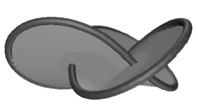
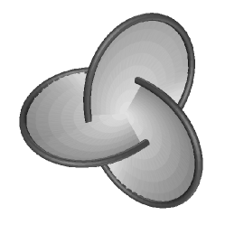
Figure 9: Two views of a cone, whose cone angle is precisely $4\pi$, on the symmetric trefoil knot from Figure 4. Computational data shows this is close to the maximum possible cone angle for this trefoil.

7 Parallel Overcrossing Number Bounds for Knots

We are now in a position to get a better lower bound for the ropelength of any nontrival knot.

Theorem 7.1.

For any nontrivial knot $K$ of unit thickness,

$$\operatorname{Len}(K)\geq 4\pi+2\pi\sqrt{\operatorname{PC}(K)}\geq 2\pi\big{(}2+\sqrt{2}\big{)}.$$

Proof 7.2.

Let $T$ be the thick tube (the unit-radius solid torus) around $K$, and let $V$ be the $C^{1}$ unit vectorfield inside $T$ as in the proof of Theorem 4.1. Using Theorem 6.7, we construct a cone surface $S$ of cone angle $4\pi$ from a point $p$ outside $T$.

Let $S^{\prime}$ be the cone defined by deleting a unit neighborhood of $\partial S$ in the intrinsic geometry of $S$. Take any $q\in K$ farthest from the cone point $p$. The intersection of $S$ with the unit normal disk $D$ to $K$ at $q$ consists only of the unit line segment from $q$ towards $p$; thus $D$ is disjoint from $S^{\prime}$.

In general, the integral curves of $V$ do not close. However, we can define a natural map from $T\smallsetminus D$ to the unit disk $D$ by flowing forward along these integral curves. This map is continuous and distance-decreasing. Restricting it to $S^{\prime}\cap T$ gives a distance-decreasing (and hence area-decreasing) map to $D$, which we will prove has unsigned degree at least $\operatorname{PC}(K)$.

          

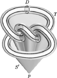
Figure 10: This trefoil knot, shown with its thick tube $T$, is coned to the point $p$ to form the cone surface $S^{\prime}$, as in the proof of Theorem 7.1. The disk $D$ is normal to the knot at the point furthest from $p$. We follow two integral curves of $V$ within $T\smallsetminus D$, through at least $\operatorname{PC}(K)$ intersections with $S^{\prime}$, until they end on $D$. Although we have drawn the curves as if they close after one trip around $T$, this is not always the case.

Note that $K^{\prime}:=\partial S^{\prime}$ is isotopic to $K$ within $T$, and thus $\operatorname{PC}(K)=\operatorname{PC}(K^{\prime})$. Furthermore, each integral curve $C$ of $V$ in $T\smallsetminus D$ can be closed by an arc within $D$ to a knot $C^{\prime}$ parallel to $K^{\prime}$. In the projection of $C^{\prime}$ and $K^{\prime}$ from the perspective of the cone point, $C^{\prime}$ must overcross $K^{\prime}$ at least $\operatorname{PC}(K^{\prime})$ times. Each of these crossings represents an intersection of $C^{\prime}$ with $S^{\prime}$. Further, each of these intersections is an intersection of $C$ with $S^{\prime}$, since the portion of $C^{\prime}$ not in $C$ is contained within the disk $D$. This proves that our area-decreasing map from $S^{\prime}\cap T$ to $D$ has unsigned degree at least $\operatorname{PC}(K)$. (An example of this map is shown in Figure 10.) Since $\operatorname{Area}(D)=\pi$ it follows that

$$\operatorname{Area}(S^{\prime})\geq\operatorname{Area}(S^{\prime}\cap T)\geq\pi\operatorname{PC}(K).$$

The isoperimetric inequality in a $4\pi$ cone is affected by the negative curvature of the cone point. However, the length $\ell$ required to surround a fixed area on $S^{\prime}$ is certainly no less than that required in the Euclidean plane:

$$\ell\geq 2\pi\sqrt{\operatorname{PC}(K)}.$$

Since each point on $K^{\prime}$ is at unit distance from $K$, we know $S^{\prime}$ is surrounded by a unit-width neighborhood inside $S$. Applying Lemma 3.1 we see that

$$\operatorname{Len}(K)\geq 4\pi+2\pi\sqrt{\operatorname{PC}(K)},$$

which by Proposition 5.4 is at least $2\pi(2+\sqrt{2})$. ∎

8 Asymptotic Crossing Number Bounds for Knots and Links

The proof of Theorem 7.1 depends on the fact that $K$ is a single knot: for a link $L$, there would be no guarantee that we could choose spanning disks $D$ for the tubes around the components of $L$ which were all disjoint from the truncated cone surface. Thus, we would be unable to close the integral curves of $V$ without (potentially) losing crossings in the process.

We can overcome these problems by using the notion of asymptotic crossing number. The essential idea of the proof is that (after a small deformation of $K$) the integral curves of $V$ will close after some number of trips around $K$. We will then be able to complete the proof as above, taking into account the complications caused by traveling several times around $K$.

For a link $L$ of $k$ components, $K_{1},\dots,K_{k}$, Freedman and He [FH] define a relative asymptotic crossing number

$$\operatorname{AC}(K_{i},L):=\inf_{pK_{i},qL}\frac{\operatorname{Ov}(pK_{i},qL)}{|pq|},$$

where the infimum is taken over all degree-$p$ satellites $pK_{i}$ of $K_{i}$ and all degree-$q$ satellites $qL$ of $L$. It is easy to see that, for each $i$,

$$\operatorname{AC}(K_{i},L)\geq\sum_{j\neq i}|\operatorname{Lk}(K_{i},K_{j})|.$$

Freedman and He also give lower bounds for this asymptotic crossing number in terms of genus, or more precisely the Thurston norm. To understand these, let $T$ be a tubular neighborhood of $L$. Then $H_{1}(\partial T)$ has a canonical basis consisting of latitudes $l_{i}$ and meridians $m_{i}$. Here, the latitudes span the kernel of the map $H_{1}(\partial T)\to H_{1}({\mathbb{R}}^{3}\smallsetminus T)$ induced by inclusion, while the meridians span the kernel of $H_{1}(\partial T)\to H_{1}(T)$.

The boundary map $H_{2}({\mathbb{R}}^{3}\smallsetminus T,\partial T)\to H_{1}(\partial T)$ is an injection; its image is spanned by the classes

$$\alpha_{i}:=l_{i}+\sum_{j\neq i}\operatorname{Lk}(K_{i},K_{j})m_{j}.$$

We now define

$$\chi_{-}(K_{i},L):=\min_{S}|S|_{T},$$

where the minimum is taken over all embedded surfaces $S$ representing the (unique) preimage of $\alpha_{i}$ in $H_{2}({\mathbb{R}}^{3}\smallsetminus T,\partial T)$, and $|S|_{T}$ is the Thurston norm of the surface $S$. That is,

$$|S|_{T}:=\sum_{S_{k}}-\chi(S_{k}),$$

where the sum is taken over all components $S_{k}$ of $S$ which are not disks or spheres, and $\chi$ is the Euler characteristic. With this definition, Freedman and He prove [FH, Thm. 4.1]:

Proposition 8.1.

If $K$ is a component of a link $L$,

$$\operatorname{AC}(K,L)\geq\chi_{-}(K,L).$$

In particular, $\operatorname{AC}(K,L)\geq 2\operatorname{genus}(K)-1$. ∎

Our interest in the asymptotic crossing number comes from the following bounds:

Theorem 8.2.

Suppose $K$ is one component of a link $L$ of unit thickness. Then

$$\operatorname{Len}(K)\geq 2\pi+2\pi\sqrt{\operatorname{AC}(K,L)}.$$

If $K$ is nontrivially knotted, this can be improved to

$$\operatorname{Len}(K)\geq 4\pi+2\pi\sqrt{\operatorname{AC}(K,L)}.$$

Proof 8.3.

As before, we use Lemma 3.3 or Theorem 6.7 to construct a cone surface $S$ of cone angle $2\pi$ or $4\pi$. We let $S^{\prime}$ be the complement of a unit neighborhood of $\partial S$, and set $K^{\prime}:=\partial S^{\prime}$, isotopic to $K$.

Our goal is to bound the area of $S^{\prime}$ below. As before, take the collection $T$ of embedded tubes surrounding the components of $L$, and let $V$ be the $C^{1}$ unit vectorfield normal to the normal disks of $T$. Fix some component $J$ of $L$ (where $J$ may be the same as $K$), and any normal disk $D$ of the embedded tube $T_{J}$ around $J$. The flow of $V$ once around the tube defines a map from $D$ to $D$. The geometry of $V$ implies that this map is an isometry, and hence this map is a rigid rotation by some angle $\theta_{J}$. Our first claim is that we can make a $C^{1}$-small perturbation of $J$ which ensures that $\theta_{J}$ is a rational multiple of $2\pi$.

Fix a particular integral curve of $V$. Following this integral curve once around $J$ defines a framing (or normal field) on $J$ which fails to close by angle $\theta_{J}$. If we define the twist of a framing $W$ on a curve $J$ by

$$\operatorname{Tw}(W)=\frac{1}{2\pi}\int\frac{dW}{ds}\times W\cdot\,\operatorname{ds},$$

it is easy to show that this framing has zero twist. We can close this framing by adding twist $-\theta_{J}/2\pi$, defining a framing $W$ on $J$. If we let $\operatorname{Wr}(J)$ be the writhe of $J$, then the Călugăreanu–White formula [Căl1, Căl2, Căl3, Whi2] tells us that $\operatorname{Lk}(J,J^{\prime})=\operatorname{Wr}(J)-\theta_{J}/2\pi$, where $J^{\prime}$ is a normal pushoff of $J$ along $W$. Since the linking number $\operatorname{Lk}(J,J^{\prime})$ is an integer, this means that $\theta_{J}$ is a rational multiple of $2\pi$ if and only if $\operatorname{Wr}(J)$ is rational. But we can alter the writhe of $J$ to be rational with a $C^{1}$-small perturbation of $J$ (see [Ful, MB] for details), proving the claim.

So we may assume that, for each component $J$ of $L$, $\theta_{J}$ is a rational multiple $2\pi p_{J}/q_{J}$ of $2\pi$. Now let $q$ be the least common multiple of the (finitely many) $q_{J}$. We will now define a distance- and area-decreasing map of unsigned degree at least $q\operatorname{AC}(K,L)$ from the intersection of $T$ and the cone surface $S^{\prime}$ to a sector of the unit disk of angle $2\pi/q$.

Any integral curve of $V$ must close after $q_{J}$ trips around $J$. Thus, the link $J^{q}$ defined by following the integral curves through $q/q_{J}$ points spaced at angle $2\pi/q$ around a normal disk to $J$ is a degree-$q$ satellite of $J$. Further, if we divide a normal disk to $J$ into sectors of angle $2\pi/q$, then $J^{q}$ intersects each sector once.

We can now define a distance-decreasing map from $S^{\prime}\cap T_{J}$ to the sector by projecting along the integral curves of $V$. Letting $L^{q}$ be the union of all the integral curves $J^{q}$, and identifying the image sectors on each disk gives a map from $S^{\prime}\cap T_{L}$ to the sector. By the definition of $\operatorname{AC}(K,L)$,

$$\operatorname{Ov}(L^{q},K^{\prime})=\operatorname{Ov}(K,L^{q})\geq q\operatorname{AC}(K,L),$$

so $L^{q}$ overcrosses $K^{\prime}$ at least $q\operatorname{AC}(K,L)$ times. Thus we have at least $q\operatorname{AC}(K,L)$ intersections between $L^{q}$ and $S^{\prime}$, as in the proof of Theorem 7.1. Since the sector has area $\pi/q$, this proves that the cone $S^{\prime}$ has area at least $\pi\operatorname{AC}(K,L)$, and thus perimeter at least $2\pi\sqrt{\operatorname{AC}(K,L)}$. The theorem then follows from Lemma 3.1 as usual. ∎

Combining this theorem with Proposition 8.1 yields:

Corollary 8.4.

For any nontrivial knot $K$ of unit thickness,

$$\operatorname{Len}(K)\geq 2\pi\Big{(}2+\sqrt{2\operatorname{genus}(K)-1}\Big{)}.$$

For any component $K$ of a link $L$ of unit thickness,

$$\hfill\operatorname{Len}(K)\geq 2\pi\big{(}1+\sqrt{\chi_{-}(K,L)}\big{)},$$

where $\chi_{-}$ is the minimal Thurston norm as above.

As we observed earlier, $\operatorname{AC}(K_{i},L)$ is at least the sum of the linking numbers of the $K_{j}$ with $K_{i}$, so Theorem 8.2 subsumes Theorem 4.1. Often, it gives more information. When the linking numbers of all $K_{i}$ and $K_{j}$ vanish, the minimal Thurston norm $\chi_{-}(K_{i},L)$ has a particularly simple interpretation: it is the least genus of any embedded surface spanning $K_{i}$ and avoiding $L$. For the Whitehead link and Borromean rings, this invariant equals one, and so these bounds do not provide an improvement over the simple-minded bound of Theorem 3.5.

To find an example where Corollary 8.4 is an improvement, we need to be able to compute the Thurston norm. McMullen has shown [McM] that the Thurston norm is bounded below by the Alexander norm, which is easily computed from the multivariable Alexander polynomial. One example he suggests is a $(2,2n)$–torus link with two components. If we replace one component $K$ by its Whitehead double, then in the new link, the other component has Alexander norm $2n-1$. Since it is clearly spanned by a disk with $2n$ punctures (or a genus $n$ surface) avoiding $K$, the Thurston norm is also $2n-1$. Figure 11 (left) shows the case $n=3$, where the Alexander polynomial is $(1+x+x^{2})^{2}(1-x)(1-y)$.

On the other hand, if $K$ is either component of the three-fold link $L$ on the right in Figure 11, we can span $K$ with a genus-two surface, so we expect that $\chi_{-}(K,L)=3$, which would also improve our ropelength estimate. However, it seems hard to compute the Thurston norm in this case. The Alexander norm in this case is zero, and even the more refined bounds of Harvey [Har] do not show the Thurston norm is any greater.

Figure 11: At the left we see the result of replacing one component of a $(2,6)$–torus link by its Whitehead double. In this link $L$, the other component has Alexander norm, and hence also Thurston norm, equal to $5$. Thus Corollary 8.4 shows the total ropelength of $L$ is at least $2\pi(3+\sqrt{5})$. For the three-fold link at the right, which is a bangle sum of three square-knot tangles, we expect the Thurston norm to be $3$ (which would give ropelength at least $4\pi(1+\sqrt{3})$), but we have not found a way to prove it is not less.

9 Asymptotic Growth of Ropelength

All of our lower bounds for ropelength have been asymptotically proportional to the square root of the number of components, linking number, parallel crossing number, or asymptotic crossing number. While our methods here provide the best known results for fairly small links, other lower bounds grow like the $\tfrac{3}{4}$ power of these complexity measures. These are of course better for larger links, as described in our paper Tight Knot Values Deviate from Linear Relation [CKS]. In particular, for a link type ${\mathcal{L}}$ with crossing number $n$, the ropelength is at least $\big{(}\tfrac{4\pi}{11}n\big{)}^{3/4}$, where the constant comes from [BS]. In [CKS] we gave examples (namely the $(k,k-1)$–torus knots and the $k$-component Hopf links, which consist of $k$ circles from a common Hopf fibration of ${\mathbb{S}}^{3}$) in which ropelength grows exactly as the $\tfrac{3}{4}$ power of crossing number.

Our Theorem 3.5 proves that for the the simple chains (Figure 1), ropelength must grow linearly in crossing number $n$. We do not know of any examples exhibiting superlinear growth, but we suspect they might exist, as described below.

To investigate this problem, consider representing a link type ${\mathcal{L}}$ with unit edges in the standard cubic lattice ${\mathbb{Z}}^{3}$. The minimum number of edges required is called the lattice number $k$ of ${\mathcal{L}}$. We claim this is within a constant factor of the ropelength $\ell$ of a tight configuration of ${\mathcal{L}}$. Indeed, given a lattice representation with $k$ edges, we can easily round off the corners with quarter-circles of radius $\tfrac{1}{2}$ to create a $C^{1,1}$ curve with length less than $k$ and thickness $\tfrac{1}{2}$, which thus has ropelength $\ell$ at most $2k$. Conversely, it is clear that any thick knot of ropelength $\ell$ has an isotopic inscribed polygon with $\mathcal{O}(\ell)$ edges and bounded angles; this can then be replaced by an isotopic lattice knot on a sufficiently small scaled copy of ${\mathbb{Z}}^{3}$. We omit our detailed argument along the lines, showing $k\leq 94\ell$, since Diao et al. [DEJvR] have recently obtained the better bound $k\leq 12\ell$.

The lattice embedding problem for links is similar to the VLSI layout problem [Lei1, Lei2], where a graph whose vertex degrees are at most $4$ must be embedded in two layers of a cubic lattice. It is known [BL] that any $n$-vertex planar graph can be embedded in VLSI layout area $\mathcal{O}\big{(}n(\log n)^{2}\big{)}$. Examples of planar $n$-vertex graphs requiring layout area at least $n\log n$ are given by the so-called trees of meshes. We can construct $n$-crossing links analogous to these trees of meshes, and we expect that they have lattice number at least $n\log n$, but it seems hard to prove this. Perhaps the VLSI methods can also be used to show that lattice number (or equivalently, ropelength) is at most $\mathcal{O}\big{(}n(\log n)^{2}\big{)}$.

Here we will give a simple proof that the ropelength of an $n$-crossing link is at most $24n^{2}$, by constructing a lattice embedding of length less than $12n^{2}$. This follows from the theorem of Schnyder [dFPP, Sch1] which says that an $n$-vertex planar graph can be embedded with straight edges connecting vertices which lie on an $(n-1)\times(n-1)$ square grid. We double this size, to allow each knot crossing to be built on a $2\times 2\times 2$ array of vertices. For an $n$-crossing link diagram, there are $2n$ edges, and we use $2n$ separate levels for these edges. Thus we embed the link in a $(2n-2)\times(2n-2)\times(2n+2)$ piece of the cubic lattice. Each edge has length less than $6n$, giving total lattice number less than $12n^{2}$.

Note that Johnston has recently given an independent proof [Joh] that an $n$-crossing knot can be embedded in the cubic grid with length $\mathcal{O}(n^{2})$. Although her constant is worse than our $12$, her embedding is (like a VLSI layout) contained in just two layers of the cubic lattice. It is tempting to think that an $\mathcal{O}(n^{2})$ bound on ropelength could be deduced from the Dowker code for a knot, and in fact such a claim appeared in [Buc]. But we do not see any way to make such an argument work.

The following theorem summarizes the results of this section:

Theorem 9.1.

Let ${\mathcal{L}}$ be a link type with minimum crossing number $n$, lattice number $k$, and minimum ropelength $\ell$. Then

$$\left(\frac{4\pi}{11}n\right)^{3/4}\,\leq\,\ell\,\leq\,2k\,\leq\,24n^{2}.\qquad\qed$$

10 Further Directions

Having concluded our results, we now turn to some open problems and conjectures.

The many examples of tight links constructed in Section 3 show that the existence and regularity results of Section 2 are in some sense optimal: we know that ropelength minimizers always exist, we cannot expect a ropelength minimizer to have global regularity better than $C^{1,1}$, and we have seen that there exist continuous families of ropelength minimizers with different shapes. Although we know that each ropelength minimizer has well-defined curvature almost everywhere (since it is $C^{1,1}$) it would be interesting to determine the structure of the singular set where the curve is not $C^{2}$. We expect this singular set is finite, and in fact:

Conjecture 10.1.

Ropelength minimizers are piecewise analytic.

The $P_{n}$ bound for the ropelength of links in Theorem 3.5 is sharp, and so cannot be improved. But there is a certain amount of slack in our other ropelength estimates. The parallel crossing number and asymptotic crossing number bounds of Section 7 and Section 8 could be immediately improved by showing:

Conjecture 10.2.

If $L$ is any knot or link, $\operatorname{AC}(L)=\operatorname{PC}(L)=\operatorname{Cr}(L)$.

For a nontrivial knot, this would increase our best estimate to $4\pi+2\pi\sqrt{3}\approx 23.45$, a little better than our current estimate of $4\pi+2\pi\sqrt{2}\approx 21.45$ (but not good enough to decide whether a knot can be tied in one foot of one-inch rope). A more serious improvement would come from proving:

Conjecture 10.3.

The intersection of the tube around a knot of unit thickness with some $4\pi$ cone on the knot contains $\operatorname{PC}(K)$ disjoint unit disks avoiding the cone point.

Note that the proof of Theorem 7.1 shows only that this intersection has the area of $\operatorname{PC}(K)$ disks. This conjecture would improve the ropelength estimate for a nontrivial knot to about $30.51$, accounting for $93\%$ of Pieranski’s numerically computed value of $32.66$ for the ropelength of the trefoil [Pie]. We can see the tightness of this proposed estimate in Figure 12.

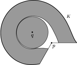
Figure 12: Pieranski’s numerically computed tight trefoil $K$ has three-fold symmetry, and there is a $4\pi$ cone point $p$ on the symmetry axis. The cone from $p$ also has three-fold symmetry, and a fundamental sector develops into a $4\pi/3$ wedge in the plane, around the point $p$. Here we show the development of that sector. The shaded regions are the intersection of the cone with the thick tube around $K$. These include a strip (of width at least $1$) inwards from the boundary $K$ of the cone, together with a disk around the unique point $q$ where $K$ cuts this sector of the cone. Our Conjecture 10.3 estimates the area of the cone from below by the area of a unit disk around $q$ plus a unit-width strip around $K$. The figure shows that the actual shaded disk and strip are not much bigger than this, and that they almost fill the sector.

Very recently, Diao has announced [Dia] a proof that the length of any unit-thickness knot $K$ satisfies

$$16\pi\operatorname{Cr}(K)\leq\operatorname{Len}(K)\big{(}\operatorname{Len}(K)-17.334\big{)}.$$

This improves our bounds in many cases. He also finds that the ropelength of a trefoil knot is greater than $24$.

Our best current bound for the ropelength of the Borromean rings is $12\pi\approx 37.70$, from Theorem 3.5. Proving only the conjecture that $\operatorname{AC}(L)=\operatorname{Cr}(L)$ would give us a fairly sharp bound on the total ropelength: If each component has asymptotic crossing number $2$, Theorem 8.2 tells us that $6\pi(1+\sqrt{2})\approx 45.51$ is a bound for ropelength. This bound would account for at least $78\%$ of the optimal ropelength, since we can exhibit a configuration with ropelength about $58.05$, built from three congruent planar curves, as in Figure 13.

Figure 13: This configuration of the Borromean rings has ropelength about $58.05$. It is built from three congruent piecewise-circular plane curves, in perpendicular planes. Each one consists of arcs from four circles of radius $2$ centered at the vertices of a rhombus of side $4$, whose major diagonal is $4$ units longer than its minor diagonal.

Although it is hard to see how to improve the ropelength of this configuration of the Borromean rings, it is not tight. In work in progress with Joe Fu, we define a notion of criticality for ropelength, and show that this configuration is not even ropelength-critical.

Finally, we observe that our cone surface methods seem useful in many areas outside the estimation of ropelength. For example, Lemma 3.3 provides the key to a new proof an unfolding theorem for space curvess:

Proposition 10.4.

For any space curve $K:S^{1}\to{\mathbb{R}}^{3}$, parametrized by arclength, there is a plane curve $K^{\prime}$ of the same length, also parametrized by arclength, so that for every $\theta$, $\phi$ in $S^{1}$,

$$|K(\theta)-K(\phi)|\leq|K^{\prime}(\theta)-K^{\prime}(\phi)|.$$

Proof 10.5.

By Lemma 3.3, there exists some cone point $p$ for which the cone of $K$ to $p$ has cone angle $2\pi$. Unrolling the cone on the plane, an isometry, constructs a plane curve $K^{\prime}$ of the same arclength. Further, each chord length of $K^{\prime}$ is a distance measured in the instrinsic geometry of the cone, which is at least the corresponding distance in ${\mathbb{R}}^{3}$. ∎

This result was proved by Reshetnyak [Res1, Res3] in a more general setting: a curve in a metric space of curvature bounded above (in the sense of Alexandrov) has an unfolding into the model two-dimensional space of constant curvature. The version for curves in Euclidean space was also proved independently by Sallee [Sal]. (In [KS], not knowing of this earlier work, we stated the result as Janse van Rensburg’s unfolding conjecture.)

The unfoldings of Reshetnyak and Sallee are always convex curves in the plane. Our cone surface method, given in the proof of Proposition 10.4, produces an unfolding that need not be convex, as shown in Figure 14. Ghomi and Howard have recently extended our argument to prove stronger results about unfoldings [GH].

Figure 14: On the left, we see a trefoil knot, with an example chord. On the right is a cone-surface unfolding of that knot, with the corresponding chord. The pictures are to the same scale, and the chord on the right is clearly longer.

We are grateful for helpful and productive conversations with many of our colleagues, including Uwe Abresch, Colin Adams, Ralph Alexander, Stephanie Alexander, Therese Biedl, Dick Bishop, Joe Fu, Mohammad Ghomi, Shelly Harvey, Zheng-Xu He, Curt McMullen, Peter Norman, Saul Schleimer and Warren Smith. We would especially like to thank Piotr Pieranski for providing the data for his computed tight trefoil, Brian White and Mike Gage for bringing Lemma 6.1 and its history to our attention, and the anonymous referee for many detailed and helpful suggestions. Our figures were produced with Geomview and Freehand. This work has been supported by the National Science Foundation through grants DMS-96-26804 (to the GANG lab at UMass), DMS-97-04949 and DMS-00-76085 (to Kusner), DMS-97-27859 and DMS-00-71520 (to Sullivan), and through a Postdoctoral Research Fellowship DMS-99-02397 (to Cantarella).

References

- [BL] Sandeep N. Bhatt and F. Thomson Leighton. A framework for solving VLSI graph layout problems. J. Comput. and Systems Sci. 28(1984), 300–343.
- [BM] Leonard M. Blumenthal and Karl Menger. Studies in Geometry. W.H. Freeman, San Francisco, 1970.
- [Buc] Greg Buck. Four-thirds power law for knots and links. Nature 392(March 1998), 238–239.
- [BS] Greg Buck and Jon Simon. Thickness and crossing number of knots. Topol. Appl. 91(1999), 245–257.
- [Căl1] George Călugăreanu. L’intégrale de Gauss et l’analyse des nœuds tridimensionnels. Rev. Math. Pures Appl. 4(1959), 5–20.
- [Căl2] George Călugăreanu. Sur les classes d’isotopie des nœuds tridimensionnels et leurs invariants. Czechoslovak Math. J. 11(1961), 588–625.
- [Căl3] George Călugăreanu. Sur les enlacements tridimensionnels des courbes fermées. Com. Acad. R. P. Romîne 11(1961), 829–832.
- [Can] Jason Cantarella. A general mutual helicity formula. R. Soc. Lond. Proc. Ser. A Math. Phys. Eng. Sci. 456(2000), 2771–2779.
- [CKKS] Jason Cantarella, Greg Kuperberg, Robert B. Kusner, and John M. Sullivan. The second hull of a knotted curve. Preprint, 2000.
- [CKS] Jason Cantarella, Robert Kusner, and John Sullivan. Tight knot values deviate from linear relation. Nature 392(1998), 237.
- [Che] Shiing Shen Chern. Curves and surfaces in euclidean space. In Shiing Shen Chern, editor, Studies in Global Geometry and Analysis, pages 16–56. Math. Assoc. Amer., 1967.
- [DS1] Isabel Darcy and De Witt Sumners. A strand passage metric for topoisomerase action. In KNOTS ’96 (Tokyo), pages 267–278. World Sci. Publishing, River Edge, NJ, 1997.
- [DS2] Isabel Darcy and De Witt Sumners. Applications of topology to DNA. In Knot theory (Warsaw, 1995), pages 65–75. Polish Acad. Sci., Warsaw, 1998.
- [dFPP] Hubert de Fraysseix, János Pach, and Richard Pollack. How to draw a planar graph on a grid. Combinatorica 10(1990), 41–51.
- [Dia] Yuanan Diao. The lower bounds of the lengths of thick knots. Preprint.
- [DEJvR] Yuanan Diao, Claus Ernst, and E. J. Janse van Rensburg. Upper bounds on linking number of thick links. J. Knot Theory Ramifications (2002). To appear.
- [ES] Michael Edelstein and Binyamin Schwarz. On the length of linked curves. Israel J. Math. 23(1976), 94–95.
- [EWW] Tobias Ekholm, Brian White, and Daniel Wienholtz. Embeddedness of minimal surfaces with total boundary curvature at most . Ann. of Math. 155(2002). To appear.
- [Fár] István Fáry. Sur la courbure totale d’une courbe gauche faisant un nœud. Bull. Soc. Math. France 77(1949), 128–138.
- [Fed] Herbert Federer. Curvature measures. Trans. Amer. Math. Soc. 93(1959), 418–491.
- [FH] Michael H. Freedman and Zheng-Xu He. Divergence free fields: energy and asymptotic crossing number. Ann. of Math. 134(1991), 189–229.
- [Ful] F. Brock Fuller. Decomposition of the linking number of a closed ribbon: a problem from molecular biology. Proc. Nat. Acad. Sci. (USA) 75(1978), 3557–3561.
- [Gag] Michael E. Gage. A proof of Gehring’s linked spheres conjecture. Duke Math. J. 47(1980), 615–620.
- [GH] Mohammad Ghomi and Ralph Howard. Unfoldings of space curves. In preparation.
- [GdlL] Oscar Gonzalez and Raphael de la Llave. Existence of ideal knots. Preprint.
- [GM] Oscar Gonzalez and John H. Maddocks. Global curvature, thickness, and the ideal shapes of knots. Proc. Nat. Acad. Sci. (USA) 96(1999), 4769–4773.
- [GM+] Oscar Gonzalez, John H. Maddocks, Friedmann Schuricht, and Heiko von der Mosel. Global curvature and self-contact of nonlinearly elastic curves and rods. Calc. Var. Partial Differential Equations 14(2002), 29–68.
- [Gro] Mikhael Gromov. Filling Riemannian manifolds. J. Diff. Geom. 18(1983), 1–147.
- [Har] Shelly L. Harvey. Higher-order polynomial invariants of 3-manifolds giving lower bounds for the Thurston norm. Preprint, 2002.
- [He] Zheng-Xu He. On the crossing number of high degree satellites of hyperbolic knots. Math. Res. Lett. 5(1998), 235–245.
- [Joh] Heather Johnston. An upper bound on the minimal edge number of an -crossing lattice knot. Preprint.
- [KBM+] Vsevolod Katritch, Jan Bednar, Didier Michoud, Robert G. Scharein, Jacques Dubochet, and Andrzej Stasiak. Geometry and physics of knots. Nature 384(November 1996), 142–145.
- [KOP+] Vsovolod Katritch, Wilma K. Olson, Piotr Pieranski, Jacques Dubochet, and Andrzej Stasiak. Properties of ideal composite knots. Nature 388(July 1997), 148–151.
- [KS] Robert B. Kusner and John M. Sullivan. On distortion and thickness of knots. In S. Whittington, D. Sumners, and T. Lodge, editors, Topology and Geometry in Polymer Science, IMA Volumes in Mathematics and its Applications, 103, pages 67–78. Springer, 1997. Proceedings of the IMA workshop, June 1996.
- [Lau] Ben Laurie. Annealing ideal knots and links: Methods and pitfalls. In A. Stasiak, V. Katritch, and L. Kauffman, editors, Ideal Knots, pages 42–51. World Scientific, 1998.
- [LKS+] Ben Laurie, Vsevolod Katritch, Jose Sogo, Theo Koller, Jacques Dubochet, and Andrzej Stasiak. Geometry and physics of catenanes applied to the study of DNA replication. Biophysical Journal 74(1998), 2815–2822.
- [Lei1] F. Thomson Leighton. Complexity Issues in VLSI. MIT Press, Cambridge, MA, 1983.
- [Lei2] F. Thomson Leighton. New lower bound techniques for VLSI. Math. Syst. Theory 17(1984), 47–70.
- [LSDR] Richard A. Litherland, Jon Simon, Oguz Durumeric, and Eric Rawdon. Thickness of knots. Topol. Appl. 91(1999), 233–244.
- [McM] Curtis T. McMullen. The Alexander polynomial of a 3-manifold and the Thurston norm on cohomology. Preprint, 2001.
- [MB] David Miller and Craig Benham. Fixed-writhe isotopies and the topological conservation law for closed, circular DNA. J. Knot Theory Ramifications 5(1996), 859–866.
- [Mil] John W. Milnor. On the total curvature of knots. Ann. of Math. 52(1950), 248–257.
- [Oss] Robert Osserman. Some remarks on the isoperimetric inequality and a problem of Gehring. J. Analyse Math. 30(1976), 404–410.
- [Pie] Piotr Pieranski. In search of ideal knots. In A. Stasiak, V. Katritch, and L. Kauffman, editors, Ideal Knots, pages 20–41. World Scientific, 1998.
- [Raw] Eric Rawdon. Approximating the thickness of a knot. In A. Stasiak, V. Katritch, and L. Kauffman, editors, Ideal Knots, pages 143–150. World Scientific, 1998.
- [Res1] Yuriĭ G. Reshetnyak. On the theory of spaces with curvature no greater than . Mat. Sb. (N.S.) 52 (94)(1960), 789–798.
- [Res2] Yuriĭ G. Reshetnyak. Inextensible mappings in a space of curvature no greater than . Siberian Math. J. 9(1968), 683–689.
- [Res3] Yuriĭ G. Reshetnyak. Nerastyagivayushchie otobrazheniya v prostranstve krivizny, ne bol~shei . Sibirsk. Mat. Ž. 9(1968), 918–927. Translated as [Res2].
- [Sal] G. Thomas Sallee. Stretching chords of space curves. Geometriae Dedicata 2(1973), 311–315.
- [Sch1] Walter Schnyder. Embedding planar graphs on the grid. In Proc. 1st ACM–SIAM Sympos. Discrete Algorithms, pages 138–148, 1990.
- [Sch2] Achill Schürmann. On extremal finite packings. Discrete Comput. Geom. (2002). To appear.
- [SDKP] Andrzej Stasiak, Jacques Dubochet, Vsevolod Katritch, and Piotr Pieranski. Ideal knots and their relation to the physics of real knots. In A. Stasiak, V. Katritch, and L. Kauffman, editors, Ideal Knots, pages 20–41. World Scientific, 1998.
- [SKB+] Andrzej Stasiak, Vsevolod Katritch, Jan Bednar, Didier Michoud, and Jacques Dubochet. Electrophoretic mobility of DNA knots. Nature 384(November 1996), 122.
- [SKK] Andrzej Stasiak, Vsovolod Katritch, and Lou Kauffman, editors. Ideal Knots. World Scientific, 1998.
- [Sum] De Witt Sumners. Lifting the curtain: using topology to probe the hidden action of enzymes. Match (1996), 51–76.
- [Thi] Morwen B. Thistlethwaite. On the Kauffman polynomial of an adequate link. Invent. Math. 93(1988), 285–296.
- [TL] Morwen B. Thistlethwaite and W. B. Raymond Lickorish. Some links with non-trivial polynomials and their crossing numbers. Comm. Math. Helv. 63(1988), 527–539.
- [Whi1] Brian White. Half of Enneper’s surface minimizes area. In Jürgen Jost, editor, Geometric Analysis and the Calculus of Variations, pages 361–367. Internat. Press, 1996.
- [Whi2] James White. Self-linking and the Gauss integral in higher dimensions. Amer. J. Math. 91(1969), 693–728.