Resolvents and Martin boundaries of product spaces

1. Introduction

Geometric scattering theory, as espoused in [19], is the study of natural operators such as the Laplacian on non-compact Riemannian manifolds $X$ with controlled asymptotic geometry using geometrically-informed, fully (i.e. to the extent it is possible) microlocal methods. The goals of this subject include the construction of an analytically useful compactification of $X$ and the definition of an appropriate class of pseudodifferential operators containing the resolvent of the Laplacian, the Schwartz kernel of which is a particularly simple distribution on this compactification. In this paper we examine the case where $X$ is a product of asymptotically hyperbolic (or conformally compact, as they are often called) spaces from this point of view. This is intended both as an initial application of these methods to higher rank symmetric spaces and their geometric generalizations, and also as a relatively simple (although still surprisingly complicated) example which should provide a guide for what to expect in further development in this area.

The results here tend to be notationally complicated, so for the purposes of this introduction we state a simple, yet representative, result concerning the asymptotics of the resolvent applied to a Schwartz function. Suppose that $(M_{j},g_{j})$, $j=1,2$, are (conformally compact) asymptotically hyperbolic, $\dim M_{j}=k_{j}+1$, $H_{j}=-\Delta_{g_{j}}$ positive, $\phi_{ji}$ are the $L^{2}$ eigenfunctions of $H_{j}$ with eigenvalue $\lambda_{ji}<k_{j}^{2}/4$. The usual compactification of $M_{j}$ as a ${\mathcal{C}}^{\infty}$ manifold with boundary is denoted $\overline{M}_{j}$, and has boundary defining function $x_{j}$. Adjoining $\rho_{j}=-1/\log x_{j}$ to the smooth structure of $\overline{M}_{j}$ yields the logarithmic blow up $(\overline{M}_{j})_{\log}$. Let $H$ be the sum of the Laplacians from the two factors: $H=H_{1}\otimes\operatorname{Id}+\operatorname{Id}\otimes H_{2}$, and $R(\mu)$ the resolvent, $(H-\mu)^{-1}$. Define

(1.1) $$\tilde{X}=[(\overline{M}_{1})_{\log}\times(\overline{M}_{2})_{\log};\partial(\overline{M}_{1})_{\log}\times\partial(\overline{M}_{2})_{\log}],$$

which is a resolution of $\overline{X}=\overline{M}_{1}\times\overline{M}_{2}$. By definition, each $\rho_{j}=-1/\log x_{j}$ is smooth on $(\overline{M}_{j})_{\log}$ and thus $\rho$, where $\rho^{-1}=\sqrt{\rho_{1}^{-2}+\rho_{2}^{-2}}$ is smooth on $\tilde{X}$.

Theorem.

(See Theorem 7.1.) Suppose $f\in\dot{\mathcal{C}}^{\infty}(\overline{X})$, $\mathbb{R}\ni\mu>k^{2}/4=(k_{1}^{2}+k_{2}^{2})/4$. Then on $\tilde{X}$:

(1.2) $$\begin{split}&R(\mu-i0)f=x_{1}^{k_{1}/2}x_{2}^{k_{2}/2}\exp(-i\sqrt{\mu-k^{2}/4}/\rho)g\\ +&\sum_{i=1}^{N_{1}}x_{2}^{k_{2}/2+i\sqrt{\mu-\lambda_{1i}-k_{2}^{2}/4}}(\phi_{1i}\otimes g_{1i})+\sum_{i=1}^{N_{2}}x_{1}^{k_{1}/2+i\sqrt{\mu-\lambda_{1i}-k_{2}^{2}/4}}(g_{2i}\otimes\phi_{2i}),\end{split}$$

$g$ polyhomogeneous on $\tilde{X}$, $g_{1i}$ and $g_{2i}$ are polyhomogeneous on $\bar{M}_{1}$ and $\bar{M}_{2}$ respectively.

The leading term of each part in the asymptotics can be described explicitly. Since $\phi_{ji}$ decays like $x_{j}^{k_{j}/2+\sqrt{k_{1}^{2}/4-\lambda_{1i}}}$, the first term dominates the other two in the interior of the front face of the blow-up (1.1); the second term, involving the eigenfunctions of $H_{1}$, is only comparable to it at the lift of $\overline{M}_{1}\times\partial\overline{M}_{2}$, while the third term, involving the eigenfunctions of $H_{2}$, is only comparable to it at the lift of $\partial\overline{M}_{1}\times\overline{M}_{2}$.

Similar results are valid outside the continuous spectrum, where the exponents are not pure imaginary, but care needs to be taken as to which eigenvalue terms appear in the asymptotics. Moreover, additional singularities appear along the front face of $\tilde{X}$ when $\mu$ is real, below the spectrum of $H$, which, however, can be resolved by further real blow-ups (or understood as a type of Legendre singularity). We refer to Theorem 6.3 for the detailed statement of the results in that case. We deduce similar results for the resolvent kernel, which we use in turn to analyze the Martin compactification ${\overline{X}}_{M}$of $M_{1}\times M_{2}$. While the latter behaves (nearly) as expected when $H_{1}$ and $H_{2}$ have no $L^{2}$ eigenvalues, it experiences a substantial collapse in the presence of such eigenvalues.

Theorem.

There is a natural continuous surjection $\tilde{X}\to{\overline{X}}_{M}$. Moreover, the following hold.

1. If neither $H_{1}$ nor $H_{2}$ have $L^{2}$ eigenvalues, the restriction of this map to a neighborhood of the front face of the blow-up in (1.1) is injective. In general, its injectivity on the ‘side faces’ of $\tilde{X}$ depends on properties of the spherical functions, i.e. on $\frac{d}{d\tau}|_{\tau=0}R_{j}(k_{j}^{2}/4+\tau^{2})$.

2. If both $H_{1}$ and $H_{2}$ have $L^{2}$ eigenvalues, the Martin boundary $\partial{\overline{X}}_{M}$ is of the form $\partial\overline{M}_{1}\cup\partial\overline{M}_{2}\cup\partial\overline{M}_{1}\times\partial\overline{M}_{2}\times I$, $I$ an open interval. This set is naturally identified with a collapsed version of $\tilde{X}$, and the map $\partial\tilde{X}\to\partial{\overline{X}}_{M}$ factors through it.

There is an extensive literature on scattering on conformally compact manifolds, including especially the important special case of convex cocompact (and geometrically finite) hyperbolic manifolds. This contains geometric constructions of the resolvent, scattering matrix and generalized eigenfunctions, as well as trace formulæ and asymptotics for the counting function for resonances. For brevity, we list only [15], [13], [14], [21], [9], [27] for references. A parallel theory for complex hyperbolic manifolds and their perturbations is initiated in [4], and while not appearing explicitly, this theory extends to manifolds with the asymptotic structure of quaternionic hyperbolic spaces and the Cayley plane.

Concerning higher rank noncompact symmetric spaces (and in less generality, their quotients too), the compactification theory is now well-understood [7], as well as at least some aspects of the analysis of the Laplacian. However, the current methods here rely heavily on the special algebraic structure of these spaces, so extensions of these results to even relatively modest geometric perturbations of these spaces are basically not understood at all.

Alongside this is the study of the asymptotically Euclidean scattering metrics initiated in [18], [20]. This theory extends the extensive classical literature, but has led to a new and detailed understanding of quantum N-body scattering where the geometry has much in common with that of flats in non-compact symmetric spaces, see e.g. [24], [8], [26] and [25].

These different geometric settings have led to the understanding of diverse analytic phenomena which may sometimes be traced to the effects of the asymptotically flat or negative curvature. One of the attractions of studying higher rank symmetric spaces from the point of view of geometric scattering theory is to isolate the specific ways in which the flat and negatively curved directions interact with one another and affect the analysis. The simplest setting where these sorts of effects might be seen is on the product $\overline{X}=\overline{M}_{1}\times\overline{M}_{2}$, where both factors $(\overline{M}_{j},g_{j})$ are conformally compact metrics. Recall that $(\overline{M},g)$ is conformally compact if $\overline{M}$ is a smooth compact manifold with boundary, such that for some defining function $x$ for $\partial\overline{M}$, $g$ takes the form $(dx^{2}+h)/x^{2}$, where $h$ is a nonnegative smooth symmetric $2$-tensor which restricts to a nondegenerate metric on $\partial\overline{M}$. (Note, however, that only the conformal class of $h$ on $\partial\overline{M}$ is well-defined from $g$.) The prototype of a conformally compact manifold is hyperbolic space, and so the prototypes for the spaces we consider here are products of hyperbolic spaces. The reader should be aware, though, that $\overline{M}_{1}\times\overline{M}_{2}$ is asymptotically like the product of hyperbolic spaces $\mathbb{H}^{n_{1}}\times\mathbb{H}^{n_{2}}$ ($n_{i}=\dim M_{i}$) only near $\partial\overline{M}_{1}\times\partial\overline{M}_{2}$, but elsewhere may be a rather severe metric and topological perturbation of this model space.

The basic questions we ask here concerning the product space $X$ with metric $g=g_{1}+g_{2}$ concern the resolvent $R_{X}(\lambda)=(\Delta_{g}-\lambda)^{-1}$ of its Laplacian $\Delta_{g}$. We sometimes write $R_{X}(\lambda)$ as $R_{g}(\lambda)$ or simply $R(\lambda)$. This is a holomorphic family of elliptic pseudodifferential operators of order $-2$ in the resolvent set $\mathbb{C}\setminus\operatorname{spec}(\Delta_{g})$, which contains at least the complement of the positive real axis. The precise extent of the spectrum is straightforward to determine from the spectra on either factor, but the first substantial question is to understand the behaviour of $R(\lambda)$ as $\lambda$ approaches the (continuous part of the) spectrum. Existence of a limit, in an appropriate sense, is known as the limiting absorption principle. Even better is the existence of a meromorphic continuation of $R(\lambda)$ beyond the spectrum. Usually, when it exists, this continuation lives on some Riemann surface covering the complex plane and ramified at the thresholds of the spectrum. Meromorphic continuations of this type are known to exist for the Laplacian of conformally compact manifolds [15]. Further important questions concern the geometric space which is a resolution of $X\times X$ obtained by a process of real blow-up, and on which the Schwartz kernel of the resolvent lives as a polyhomogeneous (or more generally, a Legendrian) distribution. Detailed knowledge of this space is central in understanding the finer properties of the resolvent, and conversely is key in its initial geometric construction. Geometric and analytic compactifications of the space $X$ itself are quite relevant to this. There are two well-known compactifications which are closely related to our methods: the geodesic (also known as the conic) compactification, and the Martin compactification, which is defined using function theory, specifically the space of positive solutions of $(\Delta_{g}-\lambda)u=0$ for $\lambda$ real and below the bottom of $\operatorname{spec}(\Delta_{g})$. This Martin compactification is known in many instances, including for the product of hyperbolic spaces [6] and more recently for general symmetric spaces of noncompact type [7]. The ‘resolvent compactification’ of $X\times X$ we construct below, and on which the Schwartz kernel of the resolvent lives, has a structure on some of its hypersurface boundary faces which is inherited from the geodesic and Martin compactifications.

These questions together have led to the somewhat modest goals of the present paper. In the next section we present a contour integral formula for $R_{X}(\lambda)$ in terms of the resolvents of the two factors $R_{M_{j}}(\lambda)$. A related expression, written as an integral over the spectral measure, derived in the context in Euclidean scattering, appears in work of Ben-Artzi and Devinatz [3]. The representation formula here holds in great generality. In §3 we specialize and review the detailed structure of the resolvent $R_{M}$ when $M$ is a conformally compact manifold; some auxiliary estimates required later are also derived here. An immediate consequence of the representation formula of §2 is the existence of an appropriate meromorphic continuation for the resolvent $R_{X}(\lambda)$, and we describe this in §4. After this, §5 contains a discussion of general compactification theory, specialized to this context. The main work is done in §6 and §7, where we describe the asymptotics of $R_{X}(\mu)f$ when $f$ is Schwartz, first when $\mu$ is in the resolvent set and then when $\mu$ is in the main sheet of continuous spectrum of $H$. The first application of this is given in §8, where we construct the ‘resolvent double space’, a resolution of $X\times X$ which carries the Schwartz kernel of $R_{X}(\mu)$ in as simple a fashion as possible. Finally, in §9, we use the resolvent asymptotics to determine the Martin compactification of $X$.

There are several features of this work to which we wish to draw particular attention. First, the main tool in deriving the resolvent asymptotics is stationary phase, which is in many respects local. The previous identification of the Martin compactification (at least for the product of hyperbolic spaces) in [6] relies heavily on global heat kernel bounds, which we feel are intrinsically more complicated. Note also that by using stationary phase we are taking advantage of the oscillatory nature of the resolvent, even when studying it for certain values of $\mu$ where it has been more traditional to rely on ‘positivity methods’ such as the maximum principle, the Harnack inequality, etc. Another interesting feature here is the surprisingly complicated way the existence of bound states, i.e. $L^{2}$ eigenvalues, for the Laplacian on either factor affects the asymptotics and the structure of the Martin boundary. Finally, we have given a detailed description of the smooth structure of the various compactifications we construct; this aspect is usually neglected in other discussions of compactification theory, but as we show, plays a significant role.

Our intention is that the investigations here will form the basis for a more thorough investigation of the geometric scattering theory for higher rank spaces.

The authors wish to thank Richard Melrose for helpful advice, and also Lizhen Ji for encouraging us to study the Martin compactification.

2. Resolvent formula

Let $H_{1}$, $H_{2}$ be self-adjoint operators on Hilbert spaces $V_{1}$ and $V_{2}$ which are bounded below; the precise structure of their spectra will be unimportant for the present. We denote $\inf\operatorname{spec}(H_{j})=\lambda_{0}(H_{j})$. Now let

$$H=H_{1}\otimes\operatorname{Id}+\operatorname{Id}\otimes H_{2}$$

be the self-adjoint operator on the completed tensor product space $V_{1}\hat{\otimes}V_{2}$. Then $\inf\operatorname{spec}(H)\equiv\lambda_{0}(H)=\lambda_{0}(H_{1})+\lambda_{0}(H_{2})$. Let

$$R_{j}(\mu_{j})=(H_{j}-\mu_{j})^{-1},\quad j=1,2,\qquad\mbox{and}\quad R(\mu)=(H-\mu)^{-1}$$

be the resolvents of the $H_{j}$ and $H$, respectively. This setting has been investigated by Ben-Artzi and Devinatz in [3], mostly from the point of view of the limiting absorption princple, i.e. the existence of the boundary values $R(\mu\pm i0)$, $\mu\in[\lambda_{0}(H_{1})+\lambda_{0}(H_{2}),\infty)$ on suitable weighted spaces, under the assumption that the limiting absorption principle holds for the $R_{j}$ individually.

One of our first goals is to show that if both $R_{j}$ admit meromorphic continuations, then $R(\mu)$ does as well. Later we wish to obtain precise asymptotics for the Schwartz kernel of $R(\mu)$ for $\mu$ in the resolvent set and in the continuous spectrum. In this section we derive a representation of $R(\mu)$ as a contour integral which will be useful for both of these purposes.

So, fix $\mu$ in the resolvent set $\mathbb{C}\setminus[\lambda_{0}(H_{1})+\lambda_{0}(H_{2}),\infty)$, and let $\gamma$ be a parametrized curve in the complex plane which is disjoint from $[\lambda_{0}(H_{1}),\infty)$ and such that $\mu-\gamma$ is disjoint from $[\lambda_{0}(H_{2}),\infty)$, or in other words, such that $\gamma$ does not intersect $[\lambda_{0}(H_{1}),\infty)\cup(\mu-[\lambda_{0}(H_{2}),\infty))$. Suppose also that $\gamma(t)=c_{\pm}t$ for $\pm t\geq T>0$ with $\operatorname{Im}c_{\pm}>0$. This is illustrated in Figure 1. The precise values of $c_{\pm}$ are unimportant for our purposes, and indeed there is considerably more leeway than this in choosing $\gamma$, but the definite separation of $\gamma$ from the spectra, ensured by $\operatorname{Im}c_{\pm}>0$, is crucial. (One can allow slighly subconic separation, but this is of no interest here.) Then we claim that

(2.1) $$R(\mu)=\frac{1}{2\pi i}\int_{\gamma}R_{1}(\mu_{1})R_{2}(\mu-\mu_{1})\,d\mu_{1}.$$

To prove this formula, first observe that since

$$\|R_{j}(\mu_{j})\|\leq|\operatorname{Im}\mu_{j}|^{-1},$$

the norm of the integrand in (2.1) (as a bounded operator on $L^{2}$) is estimated by $C(1+|t|)^{-2}$, and hence the integral converges. Next, note that it suffices to show that both sides of (2.1) produce the same result when restricted to the range of $\chi_{I}(H_{1})\otimes\operatorname{Id}$ where $I$ is any compact interval and $\chi_{I}$ its characteristic function, because the union of these ranges is dense.

Fixing the interval $I$, the integrand $R_{1}(\mu_{1})R_{2}(\mu-\mu_{2})$ is holomorphic for $\mu_{1}\notin I\cup(\mu-\operatorname{spec}(H_{2}))$. Therefore we may deform the contour to one which is the union of two curves, $\hat{\gamma}$ and $\tilde{\gamma}$, where $\hat{\gamma}$ agrees with $\gamma$ for $t\geq T^{\prime}>0$ and intersects the real axis precisely once, somewhere in $(\sup I,\infty)$, while $\tilde{\gamma}$ surrounds $I$ once. Thus

(2.2) $$\begin{split}\frac{1}{2\pi i}&\int_{\gamma}R_{1}(\mu_{1})R_{2}(\mu-\mu_{1})\,d\mu_{1}\\ &=\frac{1}{2\pi i}\int_{\hat{\gamma}}R_{1}(\mu_{1})R_{2}(\mu-\mu_{1})\,d\mu_{1}+\frac{1}{2\pi i}\int_{\tilde{\gamma}}R_{1}(\mu_{1})R_{2}(\mu-\mu_{1})\,d\mu_{1}.\end{split}$$

Figure 1. Contours of integration in the $\mu_{1}$ plane.

But now, if $\hat{\gamma}$ is moved to infinity, the first integral on the right tends to 0, as follows by directly estimating the integral. On the other hand, letting $\tilde{\gamma}$ tend to $I$ and applying Stone’s theorem, the second integral on the right is the same as

$$\int_{I}R_{2}(\mu-\mu_{1})\,dE_{1}(\mu_{1}).$$

This is identical to $R(\mu)$ on the range of $\chi_{I}(H_{1})\otimes\operatorname{Id}$ since applying $H-\mu$ to it gives (with a slight abuse of notation)

$$\int_{I}(H_{1}-\mu_{1}+H_{2}-(\mu-\mu_{1}))R_{2}(\mu-\mu_{1})\,dE_{1}(\mu_{1}).$$

$$=\int_{I}((H_{1}-\mu_{1})R_{2}(\mu-\mu_{1})+\operatorname{Id})\,dE_{1}(\mu_{1})=\int_{I}\,dE_{1}(\mu_{1})=\chi_{I}(H_{1})\otimes\operatorname{Id},$$

i.e. the identity on this subspace. Thus (2.1) is established.

3. Resolvents of conformally compact manifolds

In this section we briefly collect some facts about the resolvent family $R_{M}(\lambda)$, which we abbreviate simply as $R(\lambda)$ for the duration of this section, when $(M,g)$ is a conformally compact manifold. These are all discussed and proved in [15], to which we refer for all details.

Recall that $M$ is identified with the interior of a compact smooth manifold with boundary $\overline{M}$. The compactification $\overline{M}$ is geometrically natural: $\overline{M}$ may also be identified with the both the geodesic and Martin compactifications, as we discuss further below. Locally, $R(\lambda)$ is a pseudodifferential operator of order $-2$, but our focus is on understanding the behavior of its Schwartz kernel $K(z,z^{\prime})=K(\lambda;z,z^{\prime})$, $z,z^{\prime}\in M$, when one or both of the variables tend to infinity in $M$, i.e. to a point of $\partial M$. This can occur in various ways, of course, and the most efficient way to encode this information is to consider $K$ as a distribution on the $0$-stretched product $\overline{M}_{0}^{2}$ introduced in [15] and [13]. This space is obtained from $\overline{M}^{2}$ by blowing up the boundary of the diagonal $\partial\Delta\iota=\partial\{z=z^{\prime}\}$; equivalently, $\overline{M}^{2}_{0}=[\overline{M}^{2};\partial\Delta\iota]$ is the disjoint union of $\overline{M}^{2}\setminus\partial\Delta\iota$ with the interior spherical normal bundle of $\partial\Delta\iota$ at the corner $\partial\overline{M}\times\partial\overline{M}$, this set then being endowed with the minimal ${\mathcal{C}}^{\infty}$ structure containing the lifts of smooth functions on $\overline{M}^{2}$ and polar coordinates around $\partial\Delta\iota$.

$\overline{M}^{2}_{0}$ has three different boundary hypersurface faces: the left face which covers (indeed, is identified with) $\partial\overline{M}\times\overline{M}$, the right face which covers $\overline{M}\times\partial\overline{M}$, and the new front face covering $\partial\Delta\iota$. We denote these $B_{10}$, $B_{01}$ and $B_{11}$, and their boundary defining functions $\rho_{10}$, $\rho_{01}$ and $\rho_{11}$, respectively. Writing $z=(x,y)$ and $z^{\prime}=(x^{\prime},y^{\prime})$ near $\partial\overline{M}$, then

$$\rho_{11}=\sqrt{x^{2}+(x^{\prime})^{2}+|y-y^{\prime}|^{2}},\qquad\mbox{and}\qquad\rho_{10}=x/\rho_{11},\quad\rho_{01}=x^{\prime}/\rho_{11}.$$

If $\dim M=n=k+1$, then write $\lambda=\zeta(k-\zeta)$, where by convention the region $\mbox{\rm Re}\,\zeta>k/2$ corresponds to the resolvent set $\mathbb{C}\setminus[k^{2}/4,\infty)$ of $\Delta_{g}$. Thus for $\lambda$ in the resolvent set,

$$\zeta=k/2+i\sqrt{\lambda-k^{2}/4},$$

where the branch of the square root is chosen so that its imaginary part is negative.

Theorem 3.1.

(Mazzeo and Melrose, [15, Theorem 7.1]) For $\zeta$ in the half-plane $\mbox{\rm Re}\,\zeta>k/2$, the Schwartz kernel $K_{\zeta}$ of $R(\zeta(k-\zeta))$ is a polyhomogeneous distribution on $\overline{M}^{2}_{0}$ with the following properties. First, $R(\zeta(k-\zeta))$ has a decomposition

$$R(\zeta(k-\zeta))=R^{\prime}(\zeta(k-\zeta))+R^{\prime\prime}(\zeta(k-\zeta)),$$

where $R^{\prime}$ is an element in the small calculus $\Psi_{0}^{-2}(\overline{M})$ of $0$-pseudodifferential operators on $M$ and $R^{\prime\prime}$ is a residual element in the large calculus $\Psi_{0}^{-\infty,\zeta,\zeta}(\overline{M})$ of $0$-pseudodifferential operators. This means that the Schwartz kernel of $R^{\prime}$ has a standard polyhomogeneous singularity corresponding to pseudodifferential order $-2$ at the lifted diagonal $\Delta\iota_{0}$ in $\overline{M}_{0}^{2}$ and vanishes to infinite order along $B_{10}$ and $B_{01}$, while the Schwartz kernel of $R^{\prime\prime}$ takes the form

$$\rho_{10}^{\zeta}\rho_{01}^{\zeta}F^{\prime\prime},\quad F^{\prime\prime}\in{\mathcal{C}}^{\infty}(\overline{M}^{2}_{0};\pi_{R}^{*}\Omega_{0});$$

here $\pi_{R}^{*}\Omega_{0}$ is the lift of the 0-density bundle from the right factor (a non-vanishing section of which is given by the Riemannian density $dV_{g}$). $R(\zeta(k-\zeta))$ is holomorphic, both as a map into the space of bounded operators on $L^{2}$ and also into the space of distributions on $\overline{M}_{0}^{2}$, for $\mbox{\rm Re}\,\zeta>k/2$, and extends meromorphically, as a function with values in the space of distributions on $\overline{M}_{0}^{2}$, to the complex plane when $k$ is even, and to $\mathbb{C}\setminus-{\mathbb{N}}$ when $k$ is odd, with all poles of finite rank. Because it is constructed using only the symbol calculus, $R^{\prime}$ is holomorphic in $\lambda$. Finally, the restrictions of $\rho_{10}^{-\zeta}K_{\zeta}$ to the left face $B_{10}$ and of $\rho_{01}^{-\zeta}K_{\zeta}$ to the right face $B_{01}$ are nonvanishing for all $\zeta$ with $\mbox{\rm Re}\,\zeta>k/2$.

Remark 3.2.

It will be convenient below to write

$$K_{\zeta}=\rho_{10}^{\zeta}\rho_{01}^{\zeta}F$$

where $F$ is smooth on $\overline{M}^{2}_{0}$, apart from its conormal singularity at the lifted diagonal $\Delta\iota_{0}$.

For us, the main import of this theorem is its conclusion that $K_{\zeta}$ simple polyhomogeneous behavior on the space $\overline{M}^{2}_{0}$. One of our ultimate goals here is to find a resolution of the space $X^{2}$, where $X$ is the product of two conformally compact manifolds, on which the Schwartz kernel for the resolvent of its Laplacian is also simple.

In the next sections we shall require uniform weighted $L^{2}$ estimates for this resolvent $R(\lambda)$ as $\operatorname{Im}\lambda\to\infty$, and we now show how these follow from the parametrix construction in ([15]). We set $H=-\Delta_{g}$ here.

Theorem 3.3.

For any $s>0$ and all $\zeta$ with $\mbox{\rm Re}\,\zeta>k/2+s$ there is a constant $C_{s}$ which is independent of $\zeta$ and such that

(3.1) $$R(\zeta(k-\zeta)):x^{s}L^{2}(M,dV_{g})\longrightarrow x^{s}L^{2}(M,dV_{g})$$

is bounded and satisfies

(3.2) $$\|R(\zeta(k-\zeta))\|_{{\mathcal{B}}(x^{s}L^{2},x^{s}L^{2})}\leq\frac{C_{s}}{|\operatorname{Im}\zeta(k-\zeta)|}$$

for all $\zeta$ in this half-plane.

Proof.

The proof has a few steps. Setting $\lambda=\zeta(k-\zeta)$, the parametrix $P(\lambda)$ for $H-\lambda$ constructed in [15] satisfies

$$P(\lambda)(H-\lambda)=\operatorname{Id}+E(\lambda),\quad(H-\lambda)P(\lambda)=\operatorname{Id}+F(\lambda),$$

where $E(\lambda)$ and $F(\lambda)$ are residual, and is related to $R(\lambda)$ by the formula

(3.3) $$R(\lambda)=P(\lambda)-E(\lambda)P(\lambda)+E(\lambda)R(\lambda)F(\lambda).$$

The desired uniform estimate for $R(\lambda)$ then follows from the standard uniform $L^{2}$ estimate

$$\|R(\lambda)\|_{{\mathcal{B}}(L^{2},L^{2})}\leq\frac{1}{|\operatorname{Im}\lambda|},\qquad\lambda\in\mathbb{C}\setminus\operatorname{spec}(H),$$

and from appropriate uniform estimates for $P(\lambda)$, $E(\lambda)$ and $F(\lambda)$ in weighted spaces which we now derive.

The main work involves demonstrating a uniform estimate in weighted spaces for the resolvent of the Laplacian in hyperbolic space, and so we turn to this first. Uniform boundedness of

$$R(\zeta(k-\zeta)):x^{s}L^{2}(\mathbb{H}^{k+1};dV)\longrightarrow x^{s}L^{2}(\mathbb{H}^{k+1};dV)$$

is equivalent to the uniform boundedness of the conjugated operator $x^{-s}R(\zeta(k-\zeta))x^{s}$ on $L^{2}(\mathbb{H}^{k+1};dV)$. The Schwartz kernel of this conjugated operator is

$$K^{s}_{\zeta}(z,z^{\prime})=K^{0}_{\zeta}(z,z^{\prime})(x^{\prime}/x)^{s}=K^{0}_{\zeta}(z,z^{\prime})(\rho_{01}/\rho_{10})^{s},$$

where $K^{0}_{\zeta}(z,z^{\prime})$ is the Schwartz kernel of the resolvent of the Laplacian in ${\mathbb{H}}^{k+1}$. Recall from [15] that there is an explicit formula for $K^{0}_{\zeta}$:

(3.4) $$K^{0}_{\zeta}(\delta)=$$

$$c_{k}\left(\frac{1}{\sinh\delta}\frac{\partial\,}{\partial\delta}\right)^{\frac{k-2}{2}}\left(\frac{1}{\sinh\delta}e^{-(\zeta-k/2)\delta}\right), k\ \mbox{even},$$

$$c_{k}\int_{0}^{\infty}e^{-(\zeta-k/2)\omega}(\cosh\omega-\cosh\delta)_{+}^{-k/2}\,d\omega, k\ \mbox{odd}.$$

Here we use that the resolvent is a point-pair invariant, so $R(\lambda;z,z^{\prime})$ only involves the Riemannian (hyperbolic) distance between $z$ and $z^{\prime}$, and equivalently, may be written in terms of the elementary point-pair invariant $\delta(z,z^{\prime})$ defined by

$$\cosh\delta(z,z^{\prime})=1+\frac{|z-z^{\prime}|^{2}}{2xx^{\prime}}.$$

There are two regions in $(\mathbb{H}^{k+1})^{2}_{0}$ where $K^{s}_{\zeta}$ behaves slightly differently as $\zeta\to\infty$. These are one near the diagonal, say $\delta(z,z^{\prime})\leq 1$, and one away from the diagonal, say $\delta(z,z^{\prime})\geq 1$. We use a partition of unity to divide the Schwartz kernel into two parts. It suffices to prove $L^{2}$ boundedness of each piece separately. In the former region, $\delta(z,z^{\prime})\leq 1$, the factor $(\rho_{01}/\rho_{10})^{s}$ is bounded, independent of $\zeta$, hence the uniform $L^{2}$ boundedness of $K^{s}_{\zeta}$, and thus (3.2) can be proved just as the $L^{2}$ boundedness of $K^{0}_{\zeta}$, directly from properties of the Schwartz kernel. More explicitly, the result in this region may be deduced either by invoking the standard extension of the symbol calculus with spectral parameter, or else simply by direct calculation. On the other hand, in $\delta(z,z^{\prime})\geq 1$, $K^{s}_{\zeta}$ decays exponentially as $\zeta\to\infty$, so the additional factor $(\rho_{01}/\rho_{10})^{s}$, which takes the form $e^{s(\delta(p,z)-\delta(p,z^{\prime}))}$, where $p$ is some fixed point in the interior of $\mathbb{H}^{k+1}$, does not make much difference: the Schwartz lemma shows the desired bound (3.2) (and in fact better bounds for this piece!).

To proceed, we recall that $P(\lambda)$ is constructed in stages, and as a sum of two terms, $P(\lambda)=P_{1}(\lambda)+P_{2}(\lambda)$. Here $P_{1}(\lambda)$ is in the small calculus, and is a slight modification of the operator $P_{1}^{\prime}(\lambda)$ obtained from the use of the symbol calculus to solve away the conormal singularity along $\Delta\iota_{0}$. By standard methods, such a $P_{1}^{\prime}(\lambda)$ may be constructed so as to depend holomorphically on $\zeta\in\mathbb{C}$, and to have uniformly bounded norm on $L^{2}$. It also acts on $x^{s}L^{2}$ for each $s$, with norm depending on $s$, but not $\zeta$. Next, $P_{2}(\lambda)$ is obtained after solving away the first $\ell$ terms of the Taylor series expansion of the error term $F_{1}(\lambda)=I-(H-\lambda)P^{\prime}_{1}(\lambda)$, $F_{1}(\lambda)\in\Psi_{0}^{-\infty}(M)$, where $\ell$ is sufficiently large (greater than $s$). This approximate solution of $(H-\lambda)P_{2}(\lambda)=F_{1}(\lambda)$ is found as follows: first solve the normal equation

$$(N(H)-\lambda)N(P_{2}(\lambda))=N(F_{1}(\lambda)),$$

which is the restriction of the equation to the front face $B_{11}$. But $N(H)$ is naturally identified with the Laplacian on $\mathbb{H}^{k+1}$, and so we may apply the result of the discussion above to choose $P_{2}^{\prime}(\lambda)$ with this property, which satisfies the estimate (3.2), and such that $F_{2}^{\prime}(\lambda)=F_{1}(\lambda)-(H-\lambda)P_{1}^{\prime}(\lambda)$ vanishes to first order along $B_{11}$. Thus

$$(H-\lambda)(P_{1}^{\prime}(\lambda)+P_{2}^{\prime}(\lambda))=I-F_{2}^{\prime}(\lambda),\qquad F_{2}^{\prime}(\lambda)\in\Psi^{-\infty,\zeta+1,\zeta}_{0}(M).$$

Applying the first $\ell$ terms of the Neumann series for $(I-F_{2}^{\prime}(\lambda))^{-1}$,

$$I+S^{(\ell)}=I+F_{2}^{\prime}(\lambda)+\ldots+(F_{2}^{\prime}(\lambda))^{\ell-1}$$

on the right on both sides of this equation yields

$$(H-\lambda)(P_{1}(\lambda)+P_{2}(\lambda))=I-F_{2}(\lambda),$$

where

$$P_{j}(\lambda)=P_{j}^{\prime}(\lambda)(I+S^{(\ell)}(\lambda)),\ \ j=1,2,\quad\mbox{and}\qquad\ \ F_{2}(\lambda)\in\Psi_{0}^{-\infty,\zeta+\ell,\zeta}(M).$$

Clearly

$$\|F_{2}(\zeta(k-\zeta))\|_{{\mathcal{B}}(x^{s}L^{2},L^{2})}\leq\frac{C}{|\mbox{\rm Im}\,\zeta(k-\zeta)|},$$

with $C$ independent of $\zeta$. We also obtain a remainder term $E(\lambda)$ from applying $H-\lambda$ on the right of $P(\lambda)=P_{1}(\lambda)+P_{2}(\lambda)$, and this satisfies uniform bounds (from $L^{2}$ to $x^{s}L^{2}$) of the same form.

These facts taken all together finish the proof. ∎

4. Analytic continuation of the resolvent of $H$

In this section we shall show how to use the integral formula (2.1) to obtain an analytic continuation for the resolvent $R_{X}(\mu)=(H-\mu)^{-1}$ on $X=M_{1}\times M_{2}$ past the continuous spectrum of $H=-\Delta_{g}=H_{1}+H_{2}$. For this continuation we can either regard $R_{X}(\mu)$ as an analytic family of bounded operators between weighted $L^{2}$ spaces, or else view its Schwartz kernel as an analytic function with values in an appropriate space of distributions. The key ingredient here is the existence of similar analytic continuations for the resolvents $R_{j}(\mu)=(H_{j}-\mu)^{-1}$. Although this continuation result holds in considerably greater generality than just for products of conformally compact spaces, we shall focus exclusively on this case for the sake of being specific.

We first set up some notation. Let $\dim M_{j}=k_{j}+1$. Then it follows from Section 3, cf. also [15] that the spectrum of $H_{j}$ decomposes into the union of a band of continuous spectrum $[k_{j}^{2}/4,+\infty)$, as well as possibly a finite number of $L^{2}$ eigenvalues $\lambda_{ji}$, $i=1,\ldots,N_{j}$, $j=1,2$, in $(0,k_{j}^{2}/4)$, with the corresponding finite rank eigenprojections $\Pi_{ji}$. Next, each $R_{j}(\mu_{j})$ continues meromorphically from the resolvent set to the Riemann surface $\Sigma$ for $\sqrt{\mu_{j}-k_{j}^{2}/4}$, which we think of as two copies of $\mathbb{C}$ attached in the usual way along a cut ${\mathcal{C}}_{j}$ extending from $k_{j}^{2}/4$ to $\infty$; the resolvent set is identified with the subset of $\Sigma$ where $\operatorname{Im}\sqrt{\mu_{j}-k_{j}^{2}/4}<0$. Usually ${\mathcal{C}}_{j}$ is taken to be the ray along the positive real axis, but it will be convenient to choose it differently later. As already noted, this continuation of $R_{j}$ is either as a map into an appropriate spaces of distributions, or else for any given $s>0$, in the region $\operatorname{Im}\sqrt{\mu_{j}-k_{j}^{2}/4}<s$, as bounded operators from $x^{s}L^{2}$ to $x^{-s}L^{2}$. In any case, its poles are of finite rank, and we denote them by $\tilde{\lambda}_{ji}$, with corresponding finite rank residues $\tilde{\Pi}_{ji}$ (the tildes are meant to distinguish these from the eigendata for $H_{j}$). Note, however, that these poles of $R_{j}$ in the nonphysical part of $\Sigma$ need not be simple.

We assume until near the end of the argument that neither $H_{j}$ has any $L^{2}$ eigenvalues. Define $k$ by

$$\frac{k^{2}}{4}=\frac{k_{1}^{2}}{4}+\frac{k_{2}^{2}}{4}.$$

Then $R(\mu)$ is analytic in $\mathbb{C}\setminus[k^{2}/4,\infty)$, and we wish to show that it continues analytically past the continuous spectrum. We do this by deforming the contour of integration $\gamma$ in (2.1) in the following manner. First fix $\mu$ in the resolvent set, so that $R_{1}(\mu_{1})R_{2}(\mu-\mu_{1})$ is defined and analytic for $\mu_{1}\notin{\mathcal{C}}_{1}\cup(\mu-{\mathcal{C}}_{2})$, i.e. outside of two horizontal rays, one extending from $k_{1}^{2}/4$ to the right and the other from $\mu-k_{2}^{2}/4$ to the left. Next, rotate these cuts to rays $\tilde{\mathcal{C}}_{j}$ by pivoting them by some angle $\alpha$ counterclockwise around their endpoints. Thus we have ‘exposed’ two sectors of angle $\alpha$ from the nonphysical portion of $\Sigma$, and at the same time concealed an equal portion of the physical part of $\Sigma$. Now it is possible to deform $\gamma$ to a new contour $\gamma^{\prime}$ which lies partly in the newly uncovered sectors in $\mathbb{C}\setminus(\tilde{\mathcal{C}}_{1}\cup\tilde{\mathcal{C}}_{2})$, as in Figure 2. Finally, $\mu$ can then be moved into the nonphysical region.

Figure 2. Contour of integration to describe the analytic continuation of $R(\mu)$. In the second picture, the cuts ${\mathcal{C}}_{1}$ and ${\mathcal{C}}_{2}$, corresponding to the spectra of $H_{1}$ and $H_{2}$, respectively, have been rotated to the cuts $\tilde{\mathcal{C}}_{1}$ and $\tilde{\mathcal{C}}_{2}$. Thus near the point $\mu^{0}_{1}$ labeled here, $R_{1}(\mu^{0}_{1})$ is not a bounded operator on $L^{2}(M_{1})$. Now $\mu$, and hence $\tilde{\mathcal{C}}_{2}$ as well, can be moved upwards in the direction of the arrow.

We make this a bit more explicit. Suppose that $\mu_{0}$ is such that $\mu^{0}-k_{1}^{2}/4\neq\tilde{\lambda}_{1i}$ and $\mu^{0}-k_{2}^{2}/4\neq\tilde{\lambda}_{2i^{\prime}}$ for any $i,i^{\prime}$, and also $\mu^{0}\neq\tilde{\lambda}_{1i}+\tilde{\lambda}_{2i^{\prime}}$. Rotate the cuts ${\mathcal{C}}_{j}$ by an angle $\alpha>\arg(\mu^{0}-k_{j}^{2}/4)$, $j=1,2$. Now deform the contour $\gamma$ past $\mu^{0}-k_{2}^{2}/4$ to a new contour $\gamma^{\prime}$, such that this point is now below $\gamma^{\prime}$. During the deformation, $\gamma$ may pass through a finite number of poles of $R_{1}$, yielding residues $\tilde{\Pi}_{1i}\otimes R_{2}(\mu-\tilde{\lambda}_{1i})$. So long as $\mu$ is (sufficiently) far away from ${\mathcal{C}}_{2}$, $\mu-\mu_{1}$ is in the resolvent set of $H_{2}$, hence no poles of $R_{2}$ are encountered during this deformation. Thus we have a new representation

$$R(\mu)=\frac{1}{2\pi i}\int_{\gamma^{\prime}}R_{1}(\mu_{1})R_{2}(\mu-\mu_{1})\,d\mu_{1}-\sum_{\text{finite}}\tilde{\Pi}_{1i}\otimes R_{2}(\mu-\tilde{\lambda}_{1i}).$$

Since $\mu$ is in the resolvent set, the left hand side is still a bounded operator on $L^{2}$, although on the right hand side, one factor of the integrand $R_{1}(\mu_{1})$ is not bounded on $L^{2}$ along the entire contour.

At this point we merely have a new representation of an operator we already know exists, namely $R(\mu)$ for $\mu$ in the resolvent set, in terms of operators which are only bounded between weighted spaces. However, fixing $\gamma^{\prime}$, we can now let $\mu$ vary arbitrarily below this curve, and hence across the spectrum $[k^{2}/4,\infty)$, as long as the ramification point $k_{2}^{2}/4$ of $R_{2}$ does not lie on $\gamma^{\prime}$. When $\mu-\tilde{\lambda}_{2i}$ crosses $\gamma^{\prime}$, the residue term $-R_{1}(\mu-\tilde{\lambda}_{2i})\otimes\tilde{\Pi}_{1i}$ is produced. This yields

$$R(\mu)=\frac{1}{2\pi i}\int_{\gamma^{\prime}}R_{1}(\mu_{1})R_{2}(\mu-\mu_{1})\,d\mu_{1}$$

$$-\sum_{\text{finite}}\tilde{\Pi}_{1i}\otimes R_{2}(\mu-\tilde{\lambda}_{1i})-\sum_{\text{finite}}R_{1}(\mu-\tilde{\lambda}_{2i})\otimes\tilde{\Pi}_{2i};$$

Each of the residue terms here continue meromorphically in $\mu$ past the spectrum, with ramification points at $\tilde{\lambda}_{1i}+k_{2}^{2}/4$ (since $R_{2}$ is ramified at $k_{2}^{2}/4$) and similarly, with the indices $1$ and $2$ interchanged. These terms also have poles at $\tilde{\lambda}_{1i}+\tilde{\lambda}_{2j}$, with finite rank residues.

We have proved

Theorem 4.1.

The resolvent $R(\mu)$ for $H$ on $X=M_{1}\times M_{2}$ extends across the cut $[k^{2}/4,\infty)$ to a meromorphic function (with values in an appropriate space of distributions) on a Riemann surface ${\mathcal{T}}$ ramified at $\tilde{\lambda}_{1i}+k_{2}^{2}/4$ and $\tilde{\lambda}_{2i}+k_{1}^{2}/4$ (these points are known as Regge poles), and with finite rank poles at $\tilde{\lambda}_{1i}+\tilde{\lambda}_{2i}$.

When either $H_{1}$ or $H_{2}$ has $L^{2}$ eigenvalues, then the only difference is that $\gamma^{\prime}$ must cross these as well. Thus, the analytic continuation can be written as above, but now we must include sums over the $\lambda_{ji}$ too, and there are new ramification points at $\lambda_{1i}+k_{2}^{2}/4$ and $\lambda_{2i}+k_{1}^{2}/4$.

5. Compactification constructions

We now turn to the other major theme of this paper, which is the various ways one might compactify the conformally compact spaces $M_{j}$ or their product $X=M_{1}\times M_{2}$. The general problem of finding good compactifications of Riemannian manifolds, and in particular of (locally) symmetric spaces, has been an area of active research. We refer to [11] and [7] for more discussion of this in the symmetric space setting, and to [2] and [22] and [5] for some beautiful results in some general geometric settings.

There are two different compactication constructions we shall discuss here, the geodesic compactification (sometimes also called the conic compactification), as well as the Martin compactification. Each has a key role in understanding different aspects of the global geometry and function theory of a space. We define these now in turn.

When $Z$ is a complete, simply connected manifold of nonpositive curvature (i.e.a Cartan-Hadamard manifold), then the geodesic compactification $\overline{Z}$ is obtained by adjoining to $Z$ an ideal boundary $\partial\overline{Z}$, points of which are equivalence classes of geodesic rays. Two geodesic rays $\gamma(t)$, $\tilde{\gamma}(t)$, $t\geq 0$, are said to be equivalent if $d(\gamma(t),\tilde{\gamma}(t))$ remains bounded as $t\to\infty$. Thus in $\mathbb{R}^{n}$ any two parallel lines are identified, as are any two geodesics in the ball model of hyperbolic space $\mathbb{H}^{n}$ which converge to the same point on $S^{n-1}$. If $q\in\partial\overline{Z}$, then a neighborhood system at $q$ is given by sets of the form $(Z\setminus B_{R}(p^{\prime}))\cap\exp_{p}([T,\infty)\times{\mathcal{U}})$, where ${\mathcal{U}}$ is an open set in the unit sphere $S_{p}Z$ in $T_{p}Z$. A point on this set is on some geodesic $\gamma(t)$ emanating from $p$ with $\gamma^{\prime}(0)\in{\mathcal{U}}$ and $t\geq T$ as well as in the exterior of the ball $B_{R}(p^{\prime})$. Thus whenever $Z$ is Cartan-Hadamard, then $\overline{Z}$ is homeomorphic to a closed ball $\overline{B^{n}}$, and its boundary $\partial\overline{Z}$ is identified with the unit tangent sphere $S_{p}Z$ for any $p\in Z$. There are fairly obvious modifications of this construction when $Z$ is not necessarily simply connected, or only has nonpositive curvature outside a compact set, and then the structure of $\overline{Z}$ is more complicated, but only on account of the topology of $\mbox{int}\,Z$.

It is of substantial interest to understand when the compactification $\overline{Z}$ carries more structure than its initial definition as a topological space. In particular, we would like to determine when $\overline{Z}$ is naturally defined as a smooth manifold with boundary, or with corners. For example, When $Z=\mathbb{R}^{n}$ or $\mathbb{H}^{n}$, then as we have already stated $\overline{Z}\approx\overline{B^{n}}$, but obviously in these two examples, $\overline{Z}$ is ‘really’ a smooth closed ball. An interesting and underappreciated feature of this construction is that although it is possible to identify each of these compactifications with a ball, the smooth structures at the boundary are different, as we now explain.

When considering whether $\overline{Z}$ admits a natural smooth structure, the first key point is the regularity of the transition maps, as we now describe. Remaining within the context of Cartan-Hadamard manifolds for simplicity, the transition maps are the homeomorphisms between the unit tangent spheres at any two points $p,p^{\prime}\in Z$,

$$S_{p}Z\longrightarrow\partial\overline{Z}\longleftarrow S_{p^{\prime}}Z$$

provided through the geodesic spray from these two points. When $Z$ has curvatures bounded between two negative constants $-a^{2}$ and $-b^{2}$, then from [2] these transition maps are of Hölder class ${\mathcal{C}}^{0,\alpha}$, $\alpha=a/b$, and accordingly, in this generality, $\overline{Z}$ has only a Hölder structure. However, for either of the examples above these transition maps are smooth; this is also true for general conformally compact manifolds for suitable localized versions of these transition maps (see [13]). The other key point concerns the choice of a class of defining functions for $\partial\overline{Z}$ (or, if $\overline{Z}$ is to be regarded as a smooth manifold with corners, then for subsets of it which are identified with the various boundary hypersurfaces). Smoothness of the transition maps and choice of defining functions together determine the ${\mathcal{C}}^{\infty}$ structure on $\overline{Z}$.

There is considerable flexibility in choosing (equivalence classes of) defining functions. For $\mathbb{R}^{n}$ it is most natural to use the radial compactification with defining function for $\partial\overline{\mathbb{R}^{n}}$, $\rho_{1}=1/|z|=1/\mbox{dist}\,(z,0)$, $z\in\mathbb{R}^{n}$, the inverse of the polar distance variable. On the other hand, the Poincaré ball model for $\mathbb{H}^{n}$ suggests that the more natural choice now is $\rho_{2}=\exp(-\mbox{dist}\,(z,0))$, $0$ any fixed point in $\mathbb{H}^{n}$. These two defining functions for $\partial\overline{B^{n}}$ are quite different, since $\rho_{1}=-1/\log\rho_{2}$. We say that $(\overline{B^{n}},\rho_{1})$ is the ‘log blow-up’ of $(\overline{B^{n}},\rho_{2})$. For later reference, we shall refer to defining functions defined as the reciprocals of the Riemannian distance function or its exponential as being of polynomial or exponential type, respectively.

The difference between these polynomial and exponential type defining functions appears most clearly in the spaces of functions with polyhomogeneous behaviour at the boundary, since this involves expansions in a discrete set of complex powers of the defining function $\rho$ along with nonnegative integer powers of its logarithm, $\log\rho$. In particular, functions which are polyhomogeneous with respect to exponential-type defining functions, with all exponents having positive real part, are residual, i.e. rapidly decreasing, with respect to the log blow-up structure. The guiding principle for which defining functions to choose as primary is determined by the asymptotic behaviour of eigenfunctions of the Laplacian; one prefers eigenfunctions not to be automatically residual! The choices made above for $\overline{\mathbb{R}^{n}}$ and $\overline{\mathbb{H}^{n}}$, respectively, are vindicated by the analysis of manifolds with ‘scattering metrics’, see [19], and with conformally compact metrics, see [15] and [13].

As indicated above, the geodesic compactification of the conformally compact manifold $(M,g)$ is just $\overline{M}$ with its usual smooth structure. It is obviously of interest to identify the geodesic compactification for the product of two such manifolds, $X=M_{1}\times M_{2}$. In fact, $\partial\overline{X}$ is the simplicial join of $\partial\overline{M}_{1}$ and $\partial\overline{M}_{2}$. More specifically, it is obtained from $\partial\overline{M}_{1}\times\partial\overline{M}_{2}\times[0,\pi/2]_{\theta}$ by collapsing each $\partial\overline{M}_{1}\times\{q_{2}\}\times\{0\}$ and $\{q_{1}\}\times\partial\overline{M}_{2}\times\{\pi/2\}$ to a point. Alternatively, it can be described as the manifold with corners obtained by blowing up the corner $\partial\overline{M}_{1}\times\partial\overline{M}_{2}$ in the product $\overline{M}_{1}\times\overline{M}_{2}$, and then blowing down the $\overline{M}_{2}$ fibres in $\partial\overline{M}_{1}\times\overline{M}_{2}$ and the $\overline{M}_{1}$ fibres in $\overline{M}_{1}\times\partial\overline{M}_{2}$ in the original faces. There are three boundary hypersurfaces, $\partial\overline{M}_{1}\times M_{2}$ and $M_{1}\times\partial\overline{M}_{2}$, corresponding to limits of geodesics of the form $(\gamma_{1}(t),p_{2})$ and $(p_{1},\gamma_{2}(t))$, respectively, and also the new face $\partial\overline{M}_{1}\times\partial\overline{M}_{2}\times(0,\pi/2)$ corresponding to limits of geodesics $(\gamma_{1}(\alpha t),\gamma_{2}(\beta t))$, $\alpha^{2}+\beta^{2}=1$. It is less clear what defining functions to use for these faces, though since the ‘new face’ covering the corner comes from the two-dimensional flats, i.e. products of geodesics in each factor, it is reasonable that we should use a polynomial type defining function here. In fact, using the usual coordinates on each factor, we shall use

$$\rho_{j}=-1/\log x_{j},\quad j=1,2,\qquad r=|(\rho_{1},\rho_{2})|.$$

In other words, the smooth structure on $\overline{X}$ is the one induced from the normal blow-up at the corner of the log blow-ups of the two factors $\overline{M}_{1}$ and $\overline{M}_{2}$. The reason we use the log blow-up at all faces is that as we shall prove in the next section, the asymptotic behaviour of the resolvent involves expansions in powers of these particular defining functions.

The other compactification we consider here is due to Martin [12], and uses the function theory of $\Delta_{g}$ to associate a set of ideal boundary points $\partial Z$ to $Z$. Notably, it may be carried out in great generality for pairs $(Z,H)$ where $H$ is a semibounded self-adjoint elliptic operator on a space $Z$, though we shall always assume here that $H$ is the Laplacian. Let $\lambda_{0}=\inf\operatorname{spec}(H)$. Then for every $\lambda\in\mathbb{R}\setminus(\lambda_{0},\infty)$, there is a compactification $\overline{Z}_{M}(\lambda)$. Actually, it follows from the construction that $\overline{Z}_{M}(\lambda)$ is identified with $\overline{Z}_{M}(\lambda^{\prime})$ for any two numbers $\lambda,\lambda^{\prime}<\lambda_{0}$, so one needs to consider only $\overline{Z}_{M}(\lambda_{0})$ and any other $\overline{Z}_{M}(\lambda)$.

Fix $\lambda<\lambda_{0}$. By [23], the set of solutions $u$ to the equation $(H-\lambda)u=0$ which remain everywhere positive is nonempty; we denote this $\mathbb{R}^{+}$-invariant set by ${\mathcal{P}}_{+}(\lambda)$. The structure of this positive cone is encoded in the slice ${\mathcal{P}}_{+}^{p}(\lambda)=\{u\in{\mathcal{P}}_{+}(\lambda):u(p)=1$ for any fixed $p\in Z$. It follows readily from the Harnack inequality and elliptic estimates that for any sequence $u_{j}\in{\mathcal{P}}_{+}^{p}(\lambda)$ there is a subsequence $u_{j^{\prime}}$ converging to a point in this space, and so ${\mathcal{P}}_{+}^{p}(\lambda)$ is compact. It is also obviously convex. Let ${\mathcal{E}}$ denote the set of its extreme points. Then for any $u\in{\mathcal{P}}_{+}^{p}(\lambda)$, the Krein-Milman theorem gives a measure $dm_{u}(e)$ supported on ${\mathcal{E}}$ such that $u=\int_{\mathcal{E}}dm_{u}(e)$. This is the generalized Poisson representation theorem! The set ${\mathcal{E}}$, or ${\mathcal{E}}(Z,\lambda)$ is called the minimal Martin boundary of $Z$. If $u\in{\mathcal{E}}$, then whenever $v\in{\mathcal{P}}_{+}^{p}(\lambda)$ and $v\leq u$ then $v=cu$ for some constant $0<c\leq 1$, and this justifies the moniker ‘minimal’.

If $Z$ were to naturally embed in ${\mathcal{P}}_{+}^{p}(\lambda)$, then the closure of its image would be an obvious way to compactify it. Unfortunately, this is not the case, but instead we consider the resolvent kernel $R(\lambda;z,w)$. This is a solution of $(H_{z}-\lambda)R(\lambda;z,w)=0$ when $z\neq w$, but is singular at $z=w$ and in addition, $R(\lambda;p,w)\neq 1$. Thus we define

$$u_{w}(z)=R(\lambda,z,w)/R(\lambda,p,w),$$

so that $u_{w}(p)=1$ and $u_{w}$ is a regular solution of $(H-\lambda)u_{w}=0$ on $X\setminus\{w\}$. Now let $w_{j}$ be any sequence of points in $Z$ which leaves any compact set. Then some subsequence $u_{w_{j}^{\prime}}$ converges to an element of ${\mathcal{P}}_{+}^{p}(\lambda)$. The (full) Martin boundary is the set of equivalence classes of these sequences, or equivalently, is the set of all possible functions $u$ obtained as limits in this fashion. We label the different boundary points by $q\in\partial_{M}Z(\lambda)$, and write $u_{q}(z)$ for the corresponding limiting solution. The Martin compactification $\overline{Z}_{M}$ (or $\overline{Z}_{M}(\lambda)$) is the union of $Z$ and $\partial_{M}Z(\lambda)$. There is a metric on the set of functions $u_{w}(z)$, $w\in\overline{Z}_{M}$, given by

$$d_{p}(u_{w},u_{w^{\prime}})=\int_{B_{1}(p)}|u_{w}(z)-u_{w^{\prime}}(z)|\,dV_{g}.$$

Thus $\overline{Z}_{M}$ not only a topological space, but a metric space.

This definition must be modified when $\lambda=\lambda_{0}$ and there is an $L^{2}$ eigenfunction $u_{0}$ with eigenvalue $\lambda_{0}$, since then the resolvent kernel $R(\lambda_{0},z,w)$ does not exist. In this case $u_{0}>0$, and in fact $\mathbb{R}^{+}\cdot u_{0}={\mathcal{P}}_{+}^{p}(\lambda_{0})$, i.e. the only positive solutions are positive multiples of $u_{0}$. Hence it is consistent to let $\overline{Z}_{M}(\lambda_{0})$ be the one point compactification of $Z$ then. Otherwise, if $\lambda_{0}$ is not in the point spectrum, then the definition is the same as before.

If $Z=\mathbb{R}^{n}$, then $\lambda_{0}=0$ and it is well-known that $\partial_{M}\mathbb{R}^{n}(0)$ is a single point, so that $(\overline{\mathbb{R}^{n}})_{M}(0)$ is the one-point compactification $S^{n}$. On the other hand, for $\lambda<0$, the extreme points of ${\mathcal{P}}_{+}^{0}(\lambda)$ are the exponentials $e^{x\cdot\xi}$, $|\xi|^{2}=-\lambda$, and this sphere of radius $\sqrt{-\lambda}$ is the full Martin boundary, and so $(\overline{\mathbb{R}^{n}})_{M}(\lambda)=\bar{B}^{n}$. If $Z=\mathbb{H}^{n}$ and $n=k+1$, then $\lambda_{0}=k^{2}/4$ and $\overline{Z}_{M}(\lambda)$ is the closed ball $\overline{B^{n}}$ for all $\lambda\leq\lambda_{0}$. The minimal positive eigenfunctions are the ones of the form $x^{k/2+\sqrt{k^{2}/4-\lambda}}$ for all possible choices of upper half-space coordinates (i.e. choice of which point on the boundary of the ball to send to infinity). From [15] it follows that that when $M$ is conformally compact, $\overline{M}_{M}(\lambda)$ is still equal to $\overline{M}$. To survey other cases relevant to us in which the Martin compactification is known, when $Z$ is Cartan-Hadamard with curvatures pinched between two negative constants $-a^{2}$ and $-b^{2}$, then Anderson and Schoen [2] and Ancona [1] proved that $\overline{Z}_{M}(\lambda)=\overline{B^{n}}$ (as metric spaces). There has been recent significant progress in determining the Martin compactifications for general symmetric spaces of noncompact type; definitive results are proved in the recent monograph [7], and this has an extensive bibliography of the literature on these developments.

Of particular relevance to us here is the work of Giulini and Woess [6] where the Martin compactification of the product of two hyperbolic spaces is determined. Their result is that now $\overline{X}_{M}(\lambda)$ is identified with $[\overline{\mathbb{H}^{n_{1}}}\times\overline{\mathbb{H}^{n_{2}}};\partial\overline{\mathbb{H}^{n_{1}}}\times\partial\overline{\mathbb{H}^{n_{2}}}]$, the blow-up of the product of the two balls along the corner; recall that this space appeared as an intermediate picture in the description of the geodesic compactification. Their proof uses rather involved global heat-kernel estimates, and one of the motivations of this paper was to demonstrate how this result, and the analogous one for products of conformally compact spaces, may be obtained in a more straightforward manner using resolvent estimates and stationary phase.

To conclude this section on compactifications, we state once again that our primary interest is in obtaining a compactification of the double-space $X\times X$, where $X=M_{1}\times M_{2}$, which is natural with respect to the resolvent. More specifically, we wish that at least for $\lambda$ in the resolvent set, $R_{X}(\lambda)$ should have at most polyhomogeneous singularities at the boundary hypersurfaces of this compactification (apart from its usual diagonal singularity). This compactification is determined by examining the asymptotics of $R_{X}(\lambda;z,w)$ as the points $z=(z_{1},z_{2})$ and $w=(w_{1},w_{2})$ diverge in all possible directions. We begin the study these asymptotics in the next section. The Martin compactification is, at best, essentially a ‘slice’ of this resolvent compactification, and in any case is easily determined from this asymptotic analysis, as we do in the final section. We shall see there that when either $H_{1}$ or $H_{2}$ has eigenvalues below the continuous spectrum, then the Martin compactification of $X$ is obtained by substantially collapsing part of the boundary of the geodesic compactification $\overline{X}$, and so loses a lot of information about the fine structure of the resolvent. Thus the resolvent compactification is the primary object of interest.

6. Asymptotics

In the remainder of this paper we shall give a more detailed description of the structure of the resolvent $R(\mu)$ on $X$. As a first approach to this we adopt the more traditional viewpoint and derive the asymptotic behavior of $R(\mu)f$ when $f\in\dot{\mathcal{C}}^{\infty}(\bar{X})$. (Functions vanishing to all orders at $\partial X$ are a suitable analogue of the space of Schwartz functions.) More generally, it makes absolutely no difference if we allow $f$ to be the sum of an element of $\dot{\mathcal{C}}^{\infty}(\bar{X})$ and a distribution of compact support. In particular, all of the calculations below apply when $f=\delta_{p}$, $p\in X=M_{1}\times M_{2}$; indeed, this is the basis for our identification of the Martin boundary of $X$. However, we shall simply assume that $f$ is Schwartz, and also, in this section, that $\mu$ is in the resolvent set for $H$.

Recall our convention that when $\mu_{j}$ is in the resolvent set for $H_{j}$, then the imaginary part of $\sqrt{\mu_{j}-k_{j}^{2}/4}$ is negative, and by the results of last section, $R_{j}(\mu_{j})f$ is then of the form

$$x_{j}^{k_{j}/2+i\sqrt{\mu_{j}-k_{j}^{2}/4}}g_{j},\ g_{j}\in{\mathcal{C}}^{\infty}(\overline{M}_{j}).$$

Also, if $\phi_{ji}$ is an $L^{2}$ eigenfunction of of $H_{j}$ with eigenvalue $\lambda_{ji}$, then

$$\phi_{ji}=x_{j}^{k_{j}/2+i\sqrt{\lambda_{ji}-k_{j}^{2}/4}}g_{j},\ g_{j}\in{\mathcal{C}}^{\infty}(\overline{M}_{j});$$

the Schwartz kernel of $\Pi_{ji}$ is $\phi_{ji}(z_{j})\otimes\overline{\phi_{ji}}(z_{j}^{\prime})$ if the eigenvalue is simple, and is a finite sum of such terms otherwise.

We start with a slightly stronger result concerning the structure of $R_{12}(\mu_{1},\mu_{2})=R_{1}(\mu_{1})\otimes R_{2}(\mu_{2})$ applied to $f\in\dot{\mathcal{C}}^{\infty}(\bar{X})$, considered as a function of both $\mu_{1}$ and $\mu_{2}$. Although this follows directly from the corresponding statement in each factor if $f=f_{1}\otimes f_{2}$, $f_{j}\in\dot{\mathcal{C}}^{\infty}(\overline{M}_{j})$, it is convenient to prove the general result directly. Thus, the kernel of $R_{12}(\mu_{1},\mu_{2})$ is polyhomogeneous on $(\overline{M}_{1})^{2}_{0}\times(\overline{M}_{2})^{2}_{0}$. Let $\pi_{L}$, $\pi_{R}$ be the projections to the left and right factors of $\overline{M}_{1}\times\overline{M}_{2}$. That is, if $\pi_{L,j}$, resp. $\pi_{R,j}$, denote the projection of $(\overline{M}_{j})^{2}_{0}$ to its left factor, resp. right, factor, then $\pi_{L}=\pi_{L,1}\times\pi_{L,2}$, $\pi_{R}=\pi_{R,1}\times\pi_{R,2}$. Note that $\pi_{L}$, $\pi_{R}$, are b-fibrations. Then $R_{12}(\mu_{1},\mu_{2})$ applied to $f$ is given by the push-forward of $R_{12}(\mu_{1},\mu_{2})\pi_{R}^{*}f$ under the map $\pi_{L}$. Thus

(6.1) $$R_{12}(\mu_{1},\mu_{2})f=x_{1}^{k_{1}/2+i\sqrt{\mu_{1}-k_{1}^{2}/4}}x_{2}^{k_{2}/2+i\sqrt{\mu_{2}-k_{2}^{2}/4}}g,\ g\in{\mathcal{C}}^{\infty}(\overline{M}_{1}\times\overline{M}_{2}).$$

The dependence on $\mu_{1}$ and $\mu_{2}$ here is uniform in the strong sense that the function $g(z_{1},z_{2},\mu_{1},\mu_{2})$ appearing in (6.1) satisfies

$$g\in{\mathcal{C}}^{\infty}(\overline{M}_{1}\times\overline{M}_{2}\times(\mathbb{C}\setminus\operatorname{spec}(H_{1}))_{\mu_{1}}\times(\mathbb{C}\setminus\operatorname{spec}(H_{2}))_{\mu_{2}}),$$

with natural extensions corresponding to the meromorphic extension of the $R_{j}$. This follows directly from the usual push-forward formula [17]. Although we use this result throughout the section, we usually state arguments for simplicity as if $R_{1}$ and $R_{2}$ are applied separately to $f$. In one particular case, when analyzing $R(\mu)f$ for $\mu$ real, below $\operatorname{spec}(H)$, and when either $H_{1}$ or $H_{2}$ have $L^{2}$ eigenvalues, we need a stronger result, where $f$ is not required to be Schwartz. We postpone that discussion until it is required, see the arguments preceeding Theorem 6.3.

The asymptotic behavior of $R(\mu)f(z)$ must be analyzed in three separate regions: near $\partial\overline{M}_{1}\times M_{2}$, near $M_{1}\times\partial\overline{M}_{2}$ and near the corner $\partial\overline{M}_{1}\times\partial\overline{M}_{2}$. Using coordinates $z=(z_{1},z_{2})$, $z_{j}=(x_{j},y_{j})$, these correspond to $x_{1}\to 0$, $x_{2}\geq c>0$, or $x_{1}\geq c>0$, $x_{2}\to 0$ or $x_{1},x_{2}\to 0$, respectively.

6.1. Asymptotics at $M_{1}\times\partial\overline{M}_{2}$ and at $\partial\overline{M}_{1}\times M_{2}$

We first describe the uniform behaviour of $R(\mu)f$ on $M_{1}\times\overline{M}_{2}$, i.e. at infinity in $M_{2}$. This is given as an asymptotic series in powers of $-1/\log x_{2}$; we shall think of this later as an asymptotic expansion on the logarithmic blow-up of $\overline{M}_{2}$, which simply means that we change the ${\mathcal{C}}^{\infty}$ structure of $\overline{M}_{2}$ by replacing the defining function $x_{2}$ for the boundary by $-1/\log x_{2}$.

Suppose first that $H_{1}$ has no $L^{2}$ eigenvalues. We analyze $R(\mu)f$, using the representation (2.1) for $R(\mu)$, by shifting $\gamma$ so that it passes through $\inf\operatorname{spec}(H_{1})=k_{1}^{2}/4$, and so that the minimum of $\operatorname{Im}\sqrt{\mu-k_{2}^{2}/4-\mu_{1}}$ along this path is attained at that point, see Figure 3, and then applying (complex) stationary phase.

Figure 3. Contour of integration, $\gamma$, used to describe behavior in $M_{1}\times\overline{M}_{2}$. Here $c=\operatorname{Im}\sqrt{\mu-k^{2}/4}$, and $u_{2}=\sqrt{\mu-k_{2}^{2}/4-\mu_{1}}$.

To set things up for stationary phase, first note that $R_{2}(\mu_{2})$ maps $\dot{\mathcal{C}}^{\infty}(\overline{M}_{2})$ to $x_{2}^{k_{2}/2+i\sqrt{\mu_{2}-k_{2}^{2}/4}}{\mathcal{C}}^{\infty}(\overline{M}_{2})$. Therefore, the oscillatory factor $e^{(k_{2}/2+i\sqrt{\mu_{2}-k_{2}^{2}/4})\log x_{2}}$, $\mu_{2}=\mu-\mu_{1}$ appears in the integrand. On the other hand, $R_{1}(\mu_{1})$ is not smooth at $\mu_{1}=k_{1}^{2}/4$, but instead has an expansion in powers of $\sqrt{\mu_{1}-k_{1}^{2}/4}$. Thus it decomposes into the sum of odd and even powers, respectively, $R_{1}(\mu_{1})=R_{1}^{\text{odd}}(\mu_{1})+R_{1}^{\text{even}}(\mu_{1})$, and we write $R_{1}^{\text{odd}}(\mu_{1})=\sqrt{\mu_{1}-k_{1}^{2}/4}\,G_{1}(\mu_{1}-k_{1}^{2}/4)$ where $G_{1}$ is smooth. Because the phase $\sqrt{\mu-\mu_{1}-k_{2}^{2}/4}\,\log x_{2}$ is not stationary at $k_{1}^{2}/4$, the smooth part $R_{1}^{\text{even}}$ contributes only terms decaying faster than any power of $-1/\log x_{2}$. Thus we are left only with

$$\int_{\gamma}e^{(k_{2}/2+i\sqrt{\mu-\mu_{1}-k_{2}^{2}/4})\log x_{2}}\sqrt{\mu_{1}-k_{1}^{2}/4}\,G_{1}(\mu_{1}-k_{1}^{2}/4)\tilde{g}(\mu_{1},z,z^{\prime})\,d\mu_{1},$$

where $\tilde{g}$ is smooth in all variables. Actually, it suffices to take this integral only over some compact segment of $\gamma$ containing $k_{1}^{2}/4$ and where the decomposition of $R_{1}$ into even and odd parts is valid; using the uniform weighted $L^{2}$ estimates of §3, the integral over the remaining portion of $\gamma$ contributes a term vanishing like $x_{2}^{k_{2}/2+m}$, $m>0$ can be made as large as wished by increasing the length of the compact segment, and is therefore negligible in the asymptotics. Changing the variable of integration to $\tau=\sqrt{\mu_{1}-k_{1}^{2}/4}$, so that $\mu_{1}=k_{1}^{2}/4+\tau^{2}$, leads to

$$\int e^{(k_{2}/2+i\sqrt{\mu-k^{2}/4-\tau^{2}})\log x_{2}}2\tau^{2}G(\tau^{2})\tilde{g}(k_{1}^{2}/4+\tau^{2},z,z^{\prime})\,d\tau.$$

The phase function $\phi(\tau)=\sqrt{\mu-k^{2}/4-\tau^{2}}\log x_{2}$ is now stationary at $\tau=0$; furthermore, $\phi^{\prime\prime}(0)=-1/\sqrt{\mu-k^{2}/4}$, and so the further change of variables $\sigma=\tau\sqrt{-\log x_{2}}/(\mu-k^{2}/4)^{1/4}$ reduces this integral to

$$x_{2}^{k_{2}/2+i\sqrt{\mu-k^{2}/4}}(\mu-k^{2}/4)^{3/4}(-1/\log x_{2})^{3/2}\int e^{i\sigma^{2}/2}\hat{g}(\sigma,z,z^{\prime})\,d\sigma$$

where $\hat{g}$ is obtained from $\tilde{g}$ by replacing $\sigma$ by $\tau$. Applying the stationary phase for phase functions with nonnegative imaginary part, see [10, Theorem 7.7.5], we obtain that

(6.2) $$R(\mu)f=x_{2}^{k_{2}/2+i\sqrt{\mu-k^{2}/4}}(-1/\log x_{2})^{3/2}g,$$

where $g$ is ${\mathcal{C}}^{\infty}$ on the logarithmic blow-up $M_{1}\times(\overline{M}_{2})_{\log}$ of $M_{1}\times\overline{M}_{2}$, i.e. in the variables $(z_{1},-1/\log x_{2},y_{2})$ for $x_{1}\geq c>0$. (Of course, $g$ is continuous on $M_{1}\times\overline{M}_{2}$; it is the lower order terms in the asymptotics that necessitate the change of the smooth structure.) In fact,

$$g|_{M_{1}\times\partial\overline{M}_{2}}=\left.c\,(\mu-k^{2}/4)^{3/4}x_{2}^{-k_{2}/2-i\sqrt{\mu-k^{2}/4}}G_{1}(0)R_{2}(\mu-k_{1}^{2}/4)f\right|_{M_{1}\times\partial\overline{M}_{2}},$$

where $c$ is a constant arising from the stationary phase lemma.

There is a final simplification of this formula, arising from the fact that we can identify the operators here slightly more explicitly. First, according to [15], for each $z_{1}\in M_{1}$,

$$\left.x_{2}^{-k_{2}/2-i\sqrt{\mu-k^{2}/4}}R_{2}(\mu-k_{2}^{2}/4)f\right|_{\partial\overline{M}_{2}}$$

$$=\int_{\partial\overline{M}_{2}}P_{2}^{t}(\mu-k_{2}^{2}/4;y_{2},z_{2}^{\prime})f(z_{1},z_{2}^{\prime})\,dz_{2}^{\prime}\equiv P_{2}^{t}(\mu-k_{2}^{2}/4)(f)(z_{1},y_{2}),$$

where $P_{2}(\mu-k_{2}^{2}/4)$ is the Poisson transform on $M_{2}$ at the spectral parameter $\mu-k_{2}^{2}/4$, and $P_{2}^{t}$ its transpose. Next, by definition,

$$G_{1}(0)=\left.\frac{d\,}{d\tau}\right|_{\tau=0}R_{1}(k_{1}^{2}/4+\tau^{2}).$$

We can already see from how it was introduced that this operator arises from the non-holomorphic part of $R_{1}$, and so its Schwartz kernel is smooth on $(\overline{M}_{1})^{2}_{0}$ because the diagonal singularity of $R_{1}$, represented by $R^{\prime}_{1}$ in Theorem 3.1, does not contribute to it. However, we can see this more directly by differentiating

$$(H_{1}-k_{1}^{2}/4-\tau^{2})R_{1}(k_{1}^{2}/4+\tau^{2})=I$$

with respect to $\tau$ and setting $\tau=0$ to get $(H_{1}-k_{1}^{2}/4)G(0)=0$, and so concluding that $G_{1}(0)$ is smooth by elliptic regularity. The Schwartz kernel $G_{1}(0;z_{1},z_{1}^{\prime})$ is a familiar function on hyperbolic space: it is a non-square-integrable eigenfunction for $H_{1}$, with threshold eigenvalue $k_{1}^{2}/4$, invariant under the group of rotations which fix $z_{1}^{\prime}$, and is known as a spherical function. We shall denote it by $S_{1}(k_{1}^{2}/4;z_{1},z_{1}^{\prime})$, and regard it as a Schwartz kernel. Altogether, we have now shown that

(6.3) $$g|_{M_{1}\times\partial\overline{M}_{2}}=c\,(\mu-k^{2}/4)^{3/4}S_{1}(k_{1}^{2}/4)P_{2}^{t}(\mu-k_{2}^{2}/4)f.$$

When $H_{1}$ has $L^{2}$ eigenvalues, then shifting the contour $\gamma$ through these gives a contribution $-\Pi_{1i}\otimes R_{2}(\mu-\lambda_{1i})$ from the residues of the integrand. (For simplicity we assume that the ramification point $k_{1}^{2}/4$ is not a pole of the meromorphic continuation of $R_{1}$ to the Riemann surface, though this can obviously be handled too by the arguments preceeding Theorem 6.3.) Hence in this case we obtain

(6.4) $$\begin{split}R(\mu)f&=x_{2}^{k_{2}/2+i\sqrt{\mu-k^{2}/4}}(-1/\log x_{2})^{3/2}g\\ &\qquad+\sum_{i=1}^{N_{1}}x_{2}^{k_{2}/2+i\sqrt{\mu-\lambda_{1i}-k_{2}^{2}/4}}g_{i},\qquad\mbox{where}\ \ g,g_{i}\in{\mathcal{C}}^{\infty}(M_{1}\times(\overline{M}_{2})_{\log}).\end{split}$$

In fact, $g_{i}=\phi_{1i}\otimes\tilde{g}_{i}$, with $\tilde{g}_{i}\in{\mathcal{C}}^{\infty}(\overline{M}_{2})$ and $\phi_{1i}$ an eigenfunction of $H_{1}$ with eigenvalue $\lambda_{1i}$; indeed, $g_{i}|_{M_{1}\times\partial\overline{M}_{2}}=-(\Pi_{1i}\otimes P_{2}^{t}(\mu-\lambda_{1i}))f$.

In this region, near $M_{1}\times\partial\overline{M}_{2}$, only the $L^{2}$ eigenvalues of $H_{1}$ play a role in the asymptotics, but perhaps surprisingly, not those of $H_{2}$. Notice that all terms in (6.4) which come from the $L^{2}$ eigenvalues of $H_{1}$ dominate the term coming from the continuous spectrum since $\operatorname{Im}\sqrt{\mu-k^{2}/4}<\operatorname{Im}\sqrt{\mu-\lambda_{1i}-k_{2}^{2}/4}$. In addition, the term corresponding to the lowest eigenvalue $\lambda_{10}$ of $H_{1}$ dominates all the other terms. This will be important later in the determination of the Martin boundary in the presence of bound states.

The asymptotics of $R(\mu)f$ at the other face $\partial\overline{M}_{1}\times M_{2}$ is completely analogous. The same calculations lead to the expression

(6.5) $$\begin{split}R(\mu)f&=x_{1}^{k_{1}/2+i\sqrt{\mu-k^{2}/4}}(-1/\log x_{1})^{3/2}g\\ &\qquad+\sum_{i=1}^{N_{1}}x_{1}^{k_{1}/2+i\sqrt{\mu-\lambda_{2i}-k_{1}^{2}/4}}g_{i},\qquad\mbox{where}\ \ g,g_{i}\in{\mathcal{C}}^{\infty}((\overline{M}_{1})_{\log}\times M_{2}).\end{split}$$

In addition,

(6.6) $$g|_{\partial\overline{M}_{1}\times M_{2}}=c\,(\mu-k^{2}/4)^{3/4}P_{1}^{t}(\mu-k_{1}^{2}/4)S_{2}(k_{2}^{2}/4)f,$$

where $P_{1}^{t}$ is the transpose of the Poisson transform on $M_{1}$ and $S_{2}$ is the ‘spherical function’ at eigenvalue $k_{2}^{2}/4$ for $M_{2}$.

We note once again that even if both $H_{1}$ and $H_{2}$ have $L^{2}$ eigenvalues, only those of $H_{2}$ contribute to the asymptotics when $x_{1}\to 0$, $x_{2}\geq c>0$ and only those of $H_{1}$ contribute to the asymptotics when $x_{2}\to 0$, $x_{1}\geq c>0$. This indicates that the asymptotics at the corner $\partial\overline{M}_{1}\times\partial\overline{M}_{2}$, where both $x_{1},x_{2}\to 0$ must be more complicated, at least in the presence of bound states, because it intermediates this transition.

6.2. Asymptotics at $\partial\overline{M}_{1}\times\partial\overline{M}_{2}$ in the absence of $L^{2}$ eigenvalues

We now proceed to the analysis of $R(\mu)f$ at this corner. We have already seen that necessity of logarithmic blow ups at the side faces of the product. Correspondingly, the asymptotics at the corner necessitate that we pass to the log blow-ups of both factors $\overline{M}_{j}$, which we denote $(\overline{M}_{j})_{\log}$. In terms of these, define

$$\tilde{X}=[(\overline{M}_{1})_{\log}\times(\overline{M}_{2})_{\log};\partial(\overline{M}_{1})_{\log}\times\partial(\overline{M}_{2})_{\log}].$$

This is the correct space on which to consider asymptotics of $R(\mu)f$, as we shall now prove.

We let

$$\rho_{j}=-1/\log x_{j},\quad j=1,2,$$

be boundary defining functions of $(\overline{M}_{j})_{\log}$, and we keep denoting their pull-back to $\tilde{X}$ with the same notation. Also let $y_{1}$, $y_{2}$ denote coordinates on $\partial(\overline{M}_{j})_{\log}$, $j=1,2$. Thus, $\tilde{X}$ is the blow-up of $(\overline{M}_{1})_{\log}\times(\overline{M}_{2})_{\log}$ at the corner $\rho_{1}=\rho_{2}=0$. Hence valid coordinates in the region where $\rho_{1}/\rho_{2}<C$, for some $C>0$, are given by

$$\rho_{2},\ s=\rho_{1}/\rho_{2},\ y_{1},\ \text{and}\ y_{2}.$$

In terms of the original boundary defining functions $x_{j}$ this means that in any region where $\log x_{2}/\log x_{1}<C$, for some $C>0$, we use the projective coordinate

$$s=\frac{-1/\log x_{1}}{-1/\log x_{2}}=\frac{\log x_{2}}{\log x_{1}}$$

along the new ‘front’ face of $\tilde{X}$ covering the corner, and $-1/\log x_{2}$ as a defining function for this face. Thus $s\to 0$ upon approach to the lift of $\partial\overline{M}_{1}\times\overline{M}_{2}$, while $s\to\infty$ on approach to the lift of $\overline{M}_{1}\times\partial\overline{M}_{2}$. We note that a total boundary defining function of $\tilde{X}$ is given by

$$\rho=(\rho_{1}^{-2}+\rho_{2}^{-2})^{-1/2},$$

i.e. with the usual Euclidean notation, $r_{j}=\rho_{j}^{-1}$, $r=\rho^{-1}$, $r=\sqrt{r_{1}^{2}+r_{2}^{2}}$. This explains the appearance of $\rho^{-1}$ in our results below. In the region $s<C$, $\rho_{1}=-1/\log x_{1}$ is another total boundary defining function; it will be used for the initial local calculation and then we change to $\rho$ for the global statements. The trivial identity

$$x_{2}=e^{\log x_{2}}=e^{s\log x_{1}}=x_{1}^{s}$$

will be used repeatedly.

The integrand $R_{1}(\mu_{1})R_{2}(\mu-\mu_{1})f$ in the contour integral representation of $R(\mu)f$ has the form

$$x_{1}^{k_{1}/2+i\sqrt{\mu_{1}-k_{1}^{2}/4}}x_{2}^{k_{2}/2+i\sqrt{\mu-\mu_{1}-k_{2}^{2}/4}}g,$$

or equivalently,

(6.7) $$\exp\left\{\left[k_{1}/2+sk_{2}/2+i\left(\sqrt{\mu_{1}-k_{1}^{2}/4}+s\sqrt{\mu-\mu_{1}-k_{2}^{2}/4}\right)\right]\log x_{1}\right\}g,$$

where $g$ is ${\mathcal{C}}^{\infty}$ in $\mu,\mu_{1}$ and on $\overline{M}_{1}\times\overline{M}_{2}$. The expressions inside these square roots assume values in $\mathbb{C}\setminus[0,\infty)$, and we assume the square roots have negative imaginary parts in this region.

Suppose first that neither $H_{1}$ nor $H_{2}$ has $L^{2}$ eigenvalues. We again do a stationary phase analysis of the integral of (6.7), and for this it is necessary to choose the contour of integration so that, if we set

$$F(\mu_{1})=F_{s}(\mu_{1})=\sqrt{\mu_{1}-k_{1}^{2}/4}+s\sqrt{\mu-\mu_{1}-k_{2}^{2}/4},$$

then the supremum of $\operatorname{Im}F(\mu_{1})$ along $\gamma$ is as negative as possible. Both $\mu$ and $s$ are parameters here, and we must choose the contour differently corresponding to the different points of the front face of $\tilde{X}$, i.e. the different values of $s$. Since $F$ is analytic outside $[k_{1}^{2}/4,+\infty)\cup(\mu-[k_{2}^{2}/4,+\infty))$, its critical points and those of its imaginary part are the same. In fact, $F$ has a unique critical point, located at

(6.8) $$\mu_{1}^{0}=\mu_{1}^{0}(s)=\frac{\mu-k_{2}^{2}/4+s^{2}k_{1}^{2}/4}{1+s^{2}},$$

and this is a saddle point of the harmonic function $\operatorname{Im}F(\mu_{1})$. (We return to this and shall explain it in greater detail below.) Moreover, this critical point always lies on the straight line segment connecting the two ramification points $k_{1}^{2}/4$ and $\mu-k_{2}^{2}/4$, and tends to the former as $s\to+\infty$ and to the latter as $s\to 0$. Next,

$$F(\mu_{1}^{0})=\sqrt{(\mu-k^{2}/4)(1+s^{2})},\qquad F^{\prime}(\mu_{1}^{0})=0,$$

and

$$F^{\prime\prime}(\mu_{1}^{0})=-\frac{1}{4}s^{-2}(1+s^{2})^{5/2}(\mu-k^{2}/4)^{-3/2}.$$

Therefore we may choose an appropriate contour $\gamma$ so that $\operatorname{Im}F(\gamma(t))$ attains a non-degenerate maximum when $\gamma(t)=\mu_{1}^{0}$. The stationary phase lemma may now be applied as before, although the singular change of variables is no longer required (in $s>0$); we deduce that the asymptotics of $R(\mu)f$ have the form

(6.9) $$\begin{split}&\exp\left(\left(k_{1}/2+sk_{2}/2+i\sqrt{(\mu-k^{2}/4)(1+s^{2})}\right)\log x_{1}\right)(-1/\log x_{1})^{1/2}g\\ &=x_{1}^{k_{1}/2}x_{2}^{k_{2}/2}\left(\exp\sqrt{(\log x_{1})^{2}+(\log x_{2})^{2}}\right)^{-i\sqrt{\mu-k^{2}/4}}(-1/\log x_{1})^{1/2}g.\end{split}$$

At the points of the front face of $\tilde{X}$ where $\log x_{2}/\log x_{1}=s$ this coefficient function $g$ is a nonvanishing multiple of

$$s(1+s^{2})^{-5/4}(\mu-k^{2}/4)^{3/4}g(\mu_{1}^{0}(s))=s\,(1+s^{2})^{-5/4}((\mu-k^{2}/4)^{-3/2})^{-1/2}$$

$$\times x_{1}^{-k_{1}/2-i\sqrt{\mu_{1}^{0}(s)-k_{1}^{2}/4}}x_{2}^{-k_{2}/2-i\sqrt{\mu-\mu_{1}^{0}(s)-k_{2}^{2}/4}}R_{1}(\mu_{1}^{0}(s))R_{2}(\mu-\mu_{1}^{0}(s))f,$$

or, finally,

(6.10) $$c\,s\,(1+s^{2})^{-5/4}(\mu-k^{2}/4)^{3/4}P_{1}^{t}(\mu_{1}^{0}(s))P_{2}^{t}(\mu-\mu_{1}^{0}(s))f.$$

Note that although this computation is done separately for each value of $s$, this final expression depends smoothly on $s$ and in fact $g$ is smooth on $\tilde{X}$ up to the front face.

To be precise, we still need to examine what happens near and at the corner $s=0$, $-1/\log x_{2}=0$. However, this is hardly different from the discussion at $\partial\overline{M}_{1}\cap M_{2}$. Indeed, we simply introduce $\tau=\sqrt{\mu-\mu_{1}-k_{2}^{2}/4}$ as the new smooth variable of integration, and then stationary phase can be performed uniformly in $s$ down to $s=0$, with the limiting contour being the same as for the discussion at $\partial\overline{M}_{1}\cap M_{2}$, showing that $R(\mu)f$ is actually polyhomogeneous. In particular, note that the expansions (6.3), (6.6) and (6.10) at the front and side faces of $\tilde{X}$ match up at the corners, in agreement with the polyhomogeneity. The one point to note is that, for example, there is a factor of $(-1/\log x_{1})^{1/2}$ in (6.10), whereas (6.6) has a factor of $(-1/\log x_{1})^{3/2}$. To reconcile this, observe that (6.6) has an extra factor of $s$, and

$$s(-1/\log x_{1})^{1/2}=\frac{-\log x_{2}}{-\log x_{1}}(-1/\log x_{1})^{1/2}=(-\log x_{2})(-1/\log x_{1})^{3/2},$$

so in fact the powers match up.

We remark that if the contour $\gamma$ does not go through the critical point $\mu_{1}^{0}(s)$, then it must necessarily contain points where the integrand is larger; however, at those points the phase function itself, not just its imaginary part, will fail to be stationary, and so stationary phase gives a decay rate $O((-1/\log x)^{\infty})$; this merely indicates that the contour has not been chosen optimally and a better result is possible.

Before proceeding to the rather more subtle discussion of asymptotics at the corner in the presence of bound states, we summarize our results in their absence.

Proposition 6.1.

Suppose $f\in\dot{\mathcal{C}}^{\infty}(\overline{X})$, $\mu\in\mathbb{C}\setminus[k^{2}/4,+\infty)$, and $H_{1}$, $H_{2}$ have no $L^{2}$ eigenfunctions. Then, with $\rho_{i}=-1/\log x_{i}$, $\rho^{-1}=\sqrt{\rho_{1}^{-2}+\rho_{2}^{-2}}$, $R(\mu)f$ has the following asymptotic expansion on $\tilde{X}$:

(6.11) $$\begin{split}R(\mu)f&=x_{1}^{k_{1}/2}x_{2}^{k_{2}/2}\exp(-i\sqrt{\mu-k^{2}/4}/\rho)h.\end{split}$$

Here $h$ polyhomogeneous on $\tilde{X}$, with order $1/2$ on the front face and $3/2$ on the side faces of $\tilde{X}$. Moreover, the principal symbol of $h$ is an elliptic $f$-independent multiple of

(6.12) $$\begin{split}&P_{1}^{t}(\mu_{1}^{0}(s))P_{2}^{t}(\mu-\mu_{1}^{0}(s))f\ \text{on the front face},\\ &S_{1}(k_{1}^{2}/4)P_{2}^{t}(\mu-k_{2}^{2}/4)f\ \text{on the lift of}\ \overline{M}_{1}\times\partial\overline{M}_{2},\\ &P_{1}^{t}(\mu-k_{1}^{2}/4)S_{2}(k_{2}^{2}/4)f\ \text{on the lift of}\ \partial\overline{M}_{1}\times\overline{M}_{2},\end{split}$$

with $\mu_{1}^{0}(s)$ given by (6.8).

This discussion already indicates that $s$ plays a dual role, both as a coordinate on the space $\tilde{X}$ and also as a spectral parameter. The function $\mu_{1}^{0}(s)$ identifies the front face of $\tilde{X}$ with the line joining the two threshold values $k_{1}^{2}/4$ and $\mu-k_{2}^{2}/4$ in the spectral plane. This role becomes even more pronounced in determining asymptotics at the front face in the presence of bound states, for then the optimal locus for the contour $\gamma$ determines which of the residue terms corresponding to the different eigenvalues must be included in the asymptotics. In addition, for certain real values of $\mu$, there are a finite number of exceptional values of $s$ at which $\mu_{1}^{0}(s)$ equals either $\lambda_{1i}$ or $\mu-\lambda_{2i}$; then the optimal contour must pass through this pole, and this creates an additional Legendrian singularity. We explain all of this now.

6.3. Asymptotics at $\partial\overline{M}_{1}\times\partial\overline{M}_{2}$ in the presence of $L^{2}$ eigenvalues for $\mu\in\mathbb{C}\setminus\mathbb{R}$

Thus suppose that $H_{1}$ or $H_{2}$ have $L^{2}$ eigenvalues. As we have already seen, these correspond to poles of the integrand and the residues at these poles may contribute to the asymptotics. To see when this happens, first note that the additional terms coming from these residues have the form

(6.13) $$x_{2}^{k_{2}/2+i\sqrt{\mu-\lambda_{1i}-k_{2}^{2}/4}}\phi_{1i}\otimes\tilde{g}_{1i},\ \tilde{g}_{1i}\in{\mathcal{C}}^{\infty}(\overline{M}_{2}),$$

with analogous terms when the roles of $\overline{M}_{1}$ and $\overline{M}_{2}$ have been switched. Here

$$\phi_{1i}\in x_{1}^{k_{1}/2+i\sqrt{\lambda_{1i}-k_{1}^{2}/4}}{\mathcal{C}}^{\infty}(\overline{M}_{1}).$$

The first main observation is that the terms (6.13) dominate the previous one (LABEL:eq:corner-asymp-free-8) coming from the continuous spectrum only when

$$\operatorname{Im}\left(\sqrt{\lambda_{1i}-k_{1}^{2}/4}+s\sqrt{\mu-\lambda_{1i}-k_{2}^{2}/4}\right)>\operatorname{Im}\left(\sqrt{\mu-k^{2}/4}\sqrt{1+s^{2}}\right),$$

or in other words when

(6.14) $$\operatorname{Im}F(\lambda_{1i})>\operatorname{Im}F(\mu_{1}^{0}(s)).$$

In all other cases, these terms coming from the bound states are lower order in the expansion (LABEL:eq:corner-asymp-free-8).

To analyze this, we must examine the geometry of the function $F$ a bit more closely. Set

$$\Lambda(\mu)=\mathbb{C}\setminus\big{(}[k_{1}^{2}/4,\infty)\cup(\mu-[k_{2}^{2}/4,\infty)\big{)},$$

and let $L\subset\Lambda(\mu)$ be the open line segment connecting the two threshold values $k_{1}^{2}/4$ and $\mu-k_{2}^{2}/4$; this segment is the image of the map $(0,\infty)\ni s\to\mu_{1}^{0}(s)$. The function $F$ depends implicitly on both $\mu$ and $s$; we shall hold $\mu$ fixed throughout, but shall study how $F$ changes as $s$ varies. We have already noted that $\operatorname{Im}F$ has a saddle point at $\mu_{1}^{0}(s)$. To see this, observe first that this is the unique critical point. Next,

$$\lim_{\mu_{1}\to k_{1}^{2}/4}\operatorname{Im}F(\mu_{1})=s\operatorname{Im}\sqrt{\mu-k^{2}/4},\qquad\lim_{\mu_{1}\to\mu-k_{2}^{2}/4}\operatorname{Im}F(\mu_{1})=\operatorname{Im}\sqrt{\mu-k^{2}/4},$$

and both of these values are greater than $\operatorname{Im}F(\mu_{1}^{0}(s))=\sqrt{1+s^{2}}\operatorname{Im}\sqrt{\mu-k^{2}/4}$ since $\operatorname{Im}\sqrt{\mu-k^{2}/4}<0$. Also, each of the square roots in the expression for $F$ has imaginary part vanishing along one of the slits and tending to $-\infty$ as $\mu_{1}$ moves horizontally away from that slit, and so $\operatorname{Im}F$ tends to $-\infty$ as $|\mu_{1}|\to\infty$. Thus $\mu_{1}^{0}(s)$ is indeed a saddle point for $\operatorname{Im}F$. We make the following definition.

Definition 6.2.

For each $s$, let ${\mathcal{N}}_{s}$ and ${\mathcal{P}}_{s}$ denote the regions in $\Lambda(\mu)$ where $\operatorname{Im}F(\mu_{1})<\operatorname{Im}F(\mu_{1}^{0}(s))$ and $\operatorname{Im}F(\mu_{1})>\operatorname{Im}F(\mu_{1}^{0}(s))$, respectively.

The union of ${\mathcal{N}}_{s}$ and the slits always has one component, while ${\mathcal{P}}_{s}$ has two components, each of which has compact closure intersecting precisely one of the two slit axes and which intersect at $\mu_{1}^{0}(s)$. Label these two components ${\mathcal{P}}_{s}^{\ell}$ and ${\mathcal{P}}_{s}^{r}$, respectively, the $\ell$ and $r$ denoting whether these regions touch the slits extending toward the left or right. Finally, recall that the ‘optimal’ contour of integration $\gamma$ is any contour which remains entirely within the region ${\mathcal{N}}_{s}$, except when it passes through the saddle point.

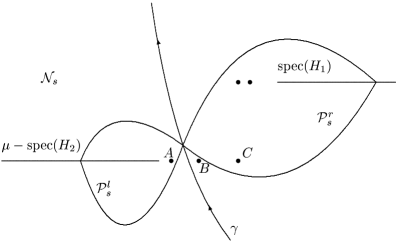
Figure 4. The regions ${\mathcal{P}}_{s}^{\ell}$, ${\mathcal{P}}_{s}^{r}$ and ${\mathcal{N}}_{s}$ for small $s>0$. The points $A$, $B$ and $C$ denote $\mu-\lambda_{23}$, $\mu-\lambda_{22}$ and $\mu-\lambda_{21}$ respectively. The contour $\gamma$ had to be shifted through point $C$, but not yet past $A$. The point $B$ can made to lie on either side of $\gamma$; the residue there gives a smaller asymptotic term than the critical point $\mu_{1}(s)$ of $F$.

Now consider the locations of the poles $\lambda_{1i}$ and $\lambda_{2i}$ relative to the contour $\gamma$ and these regions ${\mathcal{N}}_{s}$ and ${\mathcal{P}}_{s}$. For any $s$, these two collections of poles are separated by the initial choice of contour $\gamma$ in (2.1). However, in deforming $\gamma$ to a $\gamma^{\prime}$ which lies entirely within ${\mathcal{N}}_{s}$ it may be necessary to shift past some of these poles. This is not necessary if all of the $\lambda_{1i}$ lie within ${\mathcal{N}}_{s}\cup{\mathcal{P}}_{s}^{r}$ and all of the $\mu-\lambda_{2i}$ lie within ${\mathcal{N}}_{s}\cup{\mathcal{P}}_{s}^{\ell}$. When $s$ is sufficiently small, then in fact all of the $\lambda_{1i}$ lie within ${\mathcal{N}}_{s}\cup{\mathcal{P}}_{s}^{r}$; all of the $\mu-\lambda_{2i}$ lie in this region too, and none lie in ${\mathcal{P}}_{s}^{\ell}$. On the other hand, when $s\to\infty$, both the $\lambda_{1i}$ and the $\lambda_{2i}$ lie within ${\mathcal{N}}_{s}\cup{\mathcal{P}}_{s}^{\ell}$. As $s$ increases from $0$ to $\infty$, the region ${\mathcal{P}}_{s}^{\ell}$ gradually engulfs each of the points $\lambda_{1i}$, and so the optimal contour (which must always lie in ${\mathcal{N}}_{s}$) must cross these before this happens. A similar phenomenon occurs for the $\lambda_{2i}$.

6.4. Asymptotics at $\partial\overline{M}_{1}\times\partial\overline{M}_{2}$ in the presence of $L^{2}$ eigenvalues for $\mu\in\mathbb{R}$

On the other hand, when $\mu\in\mathbb{R}$ and there are bound states in the interval $(\mu-k_{2}^{2}/4,k_{1}^{2}/4)$, i.e. when

$$\mu<\min\big{\{}k_{1}^{2}/4-\max\{\lambda_{1i}\},k_{2}^{2}/4-\max\{\lambda_{2i}\}\big{\}},$$

then this analysis must fail for certain values of $s$, namely those values where either $\mu_{1}^{0}(s)=\lambda_{1i}$ or $\mu-\mu_{1}^{0}(s)=\lambda_{2i^{\prime}}$ for some $i,i^{\prime}$. For then an optimal contour would need to pass directly through a pole. It is clear that there must be some sort of jump in the behaviour at these points, because for nearby values of $s$ this phenomenon does not occur and the previous analysis may be used to get the asymptotics; the residue at the pole would be included in these asymptotics if $s$ varies slightly to one side, but are not included if it varies slightly to the other. We now prove that $R(\mu)$ has a Legendrian singularity at this front face of $\tilde{X}$ at those values of $s$ where this occurs.

To be definite, suppose that $s_{0}$ satisfies $\mu_{1}^{0}(s_{0})=\lambda_{1i}$. Let $\gamma$ be the original contour defining $R(\mu)$, as in Figure 1, and let $\gamma_{s}$ be an optimal contour for any value $s$ near $s_{0}$. We may arrange that $\gamma_{s}(0)=\mu_{1}^{0}(s)$, so $\gamma_{s_{0}}(0)=\lambda_{1i}$. When $s>s_{0}$ (closer to the lift of $\overline{M}_{1}\times\partial\overline{M}_{2}$) the contour has crossed past $\lambda_{1i}$, and the residue term is present, whereas when $s<s_{0}$ (closer to the lift of $\partial\overline{M}_{1}\times\overline{M}_{2}$) this residue term is not included.

We proceed as follows. First consider what happens when $s\to s_{0}$ from the left, i.e. with $s\leq s_{0}$. Equation (LABEL:eq:corner-asymp-free-8) describes the asymptotics when $s<s_{0}$, and we are interested in the the behavior in the limit. Write

$$R_{2}(\mu-\mu_{1})=R_{2}(\mu-\lambda_{1i})+(\mu_{1}-\lambda_{1i})\tilde{R}_{2}(\mu-\mu_{1}),$$

i.e. expand $R_{2}$ to first order in Taylor series in $\mu_{1}$ around $\mu_{1}^{0}(s_{0})=\lambda_{1i}$. Thus,

(6.15) $$\begin{split}\tilde{R}_{2}(\mu-\mu_{1})=\frac{R_{2}(\mu-\mu_{1})-R_{2}(\mu-\lambda_{1i})}{\mu_{1}-\lambda_{1i}}\\ =-\int_{0}^{1}R_{2}^{\prime}(\sigma(\mu-\mu_{1})+(1-\sigma)(\mu-\lambda_{1i}))\,d\sigma,\end{split}$$

and in particular, $\lim_{\mu_{1}\to\lambda_{1i}}\tilde{R}_{2}(\mu-\mu_{1})=-R^{\prime}_{2}(\mu-\lambda_{1i})$.

Our first remark is that the contour in $\int_{\gamma_{s}}R_{1}(\mu_{1})R_{2}(\mu-\lambda_{1i})f\,d\mu_{1}$ can be shifted farther from the spectrum of $H_{1}$ since now the $R_{2}$ term is independent of $\mu_{1}$, so its contribution is negligible. Hence we only need to analyze $\int_{\gamma_{s}}R_{1}(\mu_{1})(\mu_{1}-\lambda_{1i})\tilde{R}_{2}(\mu-\mu_{1})\,d\mu_{1}$. But

$$\tilde{R}_{1}(\mu_{1})\tilde{R}_{2}(\mu-\mu_{1})=R_{1}(\mu_{1})(\mu_{1}-\lambda_{1i})\tilde{R}_{2}(\mu-\mu_{1})$$

is holomorphic for $\mu_{1}$ near $\lambda_{1i}$, so we may move the contour to go through $\lambda_{1i}$ when $s=s_{0}$. Moreover, from the usual parametrix identity (3.3), using the holomorphy of $\tilde{R}_{1}(\mu_{1})=(\mu_{1}-\lambda_{1i})R_{1}(\mu_{1})$ as a bounded operator on $L^{2}$ near $\mu_{1}=\lambda_{1i}$, $(\mu_{1}-\lambda_{1i})R_{1}(\mu_{1})$ has the standard asymptotics. Note that $\tilde{R}_{1}(\lambda_{1i})=\Pi_{1i}$.

Thus, the holomorphic function $\tilde{R}_{1}(\mu_{1})R_{2}(\mu_{2})f$ has asymptotics

$$\tilde{R}_{1}(\mu_{1})R_{2}(\mu_{2})f=x_{1}^{k_{1}/2}x_{2}^{k_{2}/2}x_{1}^{i\sqrt{\mu_{1}-k_{1}^{2}/4}}x_{2}^{i\sqrt{\mu_{2}-k_{2}^{2}/4}}a(\mu_{1},\mu_{2}),$$

where $a(\mu_{1},\mu_{2})$ is ${\mathcal{C}}^{\infty}$ on $U_{\mu_{1}}\times U_{\mu-\mu_{2}}\times\overline{M}_{1}\times\overline{M}_{2}$, and holomorphic in $\mu_{1}$ and $\mu_{2}$, where $U$ is a neighborhood of $\lambda_{1i}$. Hence

$$\tilde{R}_{1}(\mu_{1})\tilde{R}_{2}(\mu-\mu_{1})f=\frac{\tilde{R}_{1}(\mu_{1})R_{2}(\mu-\mu_{1})f-\tilde{R}_{1}(\mu_{1})R_{2}(\mu-\lambda_{1i})f}{\mu_{1}-\lambda_{1i}}$$

$$=x_{1}^{k_{1}/2}x_{2}^{k_{1}/2}\cdot(\mu_{1}-\lambda_{1i})^{-1}\cdot\left(x_{1}^{i\sqrt{\mu_{1}-k_{1}^{2}/4}}x_{2}^{i\sqrt{\mu-\mu_{1}-k_{2}^{2}/4}}a(\mu_{1},\mu-\mu_{1})\right.$$

$$\left.-x_{1}^{i\sqrt{\mu_{1}-k_{1}^{2}/4}}x_{2}^{i\sqrt{\mu-\lambda_{1i}-k_{2}^{2}/4}}a(\mu_{1},\mu-\lambda_{1i})\right)$$

Now add and subtract $x_{1}^{i\sqrt{\mu_{1}-k_{1}^{2}/4}}x_{2}^{i\sqrt{\mu-\mu_{1}-k_{2}^{2}/4}}a(\mu_{1},\mu-\lambda_{1i})$ in the numerator of this fraction on the right, and note that the term involving the holomorphic function

$$\frac{a(\mu_{1},\mu-\mu_{1})-a(\mu_{1},\mu-\lambda_{1i})}{\mu_{1}-\lambda_{1i}}$$

has the same asymptotics as if $\lambda_{1i}$ were not a pole; thus we only need to consider

$$\int_{\gamma_{s}}\frac{x_{1}^{i\sqrt{\mu_{1}-k_{1}^{2}/4}}x_{2}^{i\sqrt{\mu-\mu_{1}-k_{2}^{2}/4}}-x_{1}^{i\sqrt{\mu_{1}-k_{1}^{2}/4}}x_{2}^{i\sqrt{\mu-\lambda_{1i}-k_{2}^{2}/4}}}{\mu_{1}-\lambda_{1i}}\,a(\mu_{1},\mu-\lambda_{1i})\,d\mu_{1}.$$

We can also write $a(\mu_{1},\mu-\lambda_{1i})=a(\lambda_{1i},\mu-\lambda_{1i})+(\mu_{1}-\lambda_{1i})a_{1}(\mu_{1},\mu-\lambda_{1i})$, where $a_{1}$ is holomorphic in $\mu_{1}$ and smooth on $\overline{M}_{1}\times\overline{M}_{2}$; the term involving $a_{1}$ again yields an expression with the standard asymptotics, as if $\lambda_{1i}$ were not a pole. Hence it remains to consider

$$a(\lambda_{1i},\mu-\lambda_{1i})\int_{\gamma_{s}}\frac{x_{1}^{i\sqrt{\mu_{1}-k_{1}^{2}/4}}x_{2}^{i\sqrt{\mu-\mu_{1}-k_{2}^{2}/4}}-x_{1}^{i\sqrt{\mu_{1}-k_{1}^{2}/4}}x_{2}^{i\sqrt{\mu-\lambda_{1i}-k_{2}^{2}/4}}}{\mu_{1}-\lambda_{1i}}\,d\mu_{1}.$$

This depends on $f$ only via

$$\begin{split}a(\lambda_{1i},\mu-\lambda_{1i})&=-x_{1}^{-k_{1}/2-i\sqrt{\lambda_{1i}-k_{1}^{2}/4}}x_{2}^{-k_{2}/2-i\sqrt{\mu-\lambda_{1i}-k_{2}^{2}/4}}(\Pi_{1i}\otimes R_{2}(\mu-\lambda_{1i}))f\\ &=-x_{1}^{-k_{1}/2-i\sqrt{\lambda_{1i}-k_{1}^{2}/4}}(\Pi_{1i}\otimes P_{2}^{t}(\mu-\lambda_{1i}))f.\end{split}$$

The factor $x_{1}^{-i\sqrt{\lambda_{1i}-k_{1}^{2}/4}}$ here corresponds to the precise decay of the eigenfunction $\phi_{1i}$. The remaining integral is an explicit function which depends only on $s$, $x_{1}$ and $x_{2}$ (and of course $\mu$). Note that in the region $x_{2}>0$, it is simply a smooth function of $s$, and $x_{2}$ (or equivalently, $s$ and $x_{1}$, keeping in mind that $s=\log x_{2}/\log x_{1}$ is near $s_{0}\in(0,+\infty)$. Thus we only need to understand the asymptotics of this function as $x_{1},x_{2}\to 0$.

Factor out $x_{1}^{iF(\mu_{1})}=x_{1}^{iF(\mu_{1}^{0}(s))}x_{1}^{i(F(\mu_{1})-F(\mu_{1}^{0}(s)))}$ to get

(6.16) $$x_{1}^{iF(\mu_{1}^{0}(s))}\int_{\gamma_{s}}e^{-i(F(\mu_{1})-F(\mu_{1}^{0}(s)))/\rho_{1}}\frac{1-e^{-is(\sqrt{\mu-\lambda_{1i}-k_{2}^{2}/4}-\sqrt{\mu-\mu_{1}-k_{2}^{2}/4})/\rho_{1}}}{\mu_{1}-\lambda_{1i}}\,d\mu_{1},$$

where we wrote the integrand in terms of $\rho_{1}=-1/\log x_{1}\geq 0$ to keep the signs easier to follow. Note that $\operatorname{Im}(F(\mu_{1})-F(\mu_{1}^{0}(s)))\leq 0$ along $\gamma_{s}$.

So far any contour $\gamma_{s}$ that stays in ${\mathcal{N}}_{s}$ has been suitable for our calculations. Now we impose an additional condition, namely that there exists a fixed interval $[-\epsilon,\epsilon]$ such that for $s_{0}-\delta\leq s\leq s_{0}$ $\gamma_{s}$ stays in the region where $\operatorname{Im}\sqrt{\mu-\mu_{1}-k_{2}^{2}/4}\geq\operatorname{Im}\sqrt{\mu-\lambda_{1i}-k_{2}^{2}/4}$. Since this region is one side of a parabola, see Figure 3, this condition can be easily satisfied. This condition ensures that the real part of the exponent in the numerator in (6.16) is non-positive, hence bounded even as $\rho_{1}\to 0$. In addition, the fraction in (6.16) is bounded by $C\rho_{1}^{-1}$ for some $C>0$, since dividing the denominator by $\rho_{1}$ yields a bounded function.

The key point is that

$$F(\mu_{1})-F(\mu_{1}^{0}(s))=(\mu_{1}-\mu_{1}^{0}(s))^{2}F_{2}(\mu_{1}-\mu_{1}^{0}(s),\mu_{1}^{0}(s)),$$

with $F_{2}$ non-zero at $(0,\mu_{1}^{0}(s))$, since $\mu_{1}^{0}(s)$ is a non-degenerate critical point of $F$, while

$$\begin{split}\sqrt{\mu-\lambda_{1i}-k_{2}^{2}/4}-\sqrt{\mu-\mu_{1}-k_{2}^{2}/4}=(\mu_{1}-\lambda_{1i})F_{1}(\mu_{1}-\lambda_{1i})\end{split}$$

with $F_{1}$ nonvanishing and holomorphic near $0$. This implies that the first exponent is a smooth function of $(\mu_{1}-\mu_{1}^{0}(s))^{2}/\rho_{1}$, with a negative real part of the same order of magnitude as $\rho_{1}\to 0$, hence Schwartz as $(\mu_{1}-\mu_{1}^{0}(s))^{2}/\rho_{1}\to\infty$, and the second one is a smooth function of $(\mu_{1}-\lambda_{1i})/\rho_{1}$ with a negative real part. However, we can only make the Schwartz conclusion here if the real part of the same order of magnitude as $(\mu_{1}-\lambda_{1i})/\rho_{1}$. Since $\gamma_{s}$ is on one side of a parabola, this is impossible to accomplish if $\gamma_{s}$ is to be smooth (for then it is tangent to the parabola). Hence, we need to break up $\gamma_{s}$ into two integrals which will yield boundary terms. These boundary terms cancel when $s\neq s_{0}$.

The geometry is as follows. Start with the space $Z_{0}=[0,1)_{\rho_{1}}\times(s_{0}-\delta,s_{0}]_{s}\times\mathbb{R}_{t}$. We first blow up $t=0$, $\rho_{1}=0$ parabolically (recall that $t$ is the parameter along $\gamma_{s}$; $\gamma_{s}(0)=\mu_{1}^{0}(s)$), so that in the interior of the front face $s$, $t/\rho_{1}^{1/2}$ and $\rho_{1}$ become valid coordinates. Then $(F(\mu_{1})-F(\mu_{1}^{0}(s)))/\rho_{1}$ is smooth near the interior of the front face, and $e^{i(F(\mu_{1})-F(\mu_{1}^{0}(s)))/\rho_{1}}$ is smooth on the blown up space with infinite order vanishing off the front face. Away from $s=s_{0}$, $e^{-is(\sqrt{\mu-\lambda_{1i}-k_{2}^{2}/4}-\sqrt{\mu-\mu_{1}-k_{2}^{2}/4})/\rho_{1}}$ is rapidly decreasing, hence the standard push-forward theorem for polyhomogeneous functions [17] yields the same result as stationary phase. In fact, we should think of integrating densities, hence we need to change $d\mu_{1}$, i.e. $dt$, to $\rho^{1/2}d(t/\rho^{1/2})$, giving the stationary phase asymptotics $\rho^{1/2}$ times a smooth function of $(s,\rho^{1/2})$ (multiplied by the exponential $x_{1}^{iF(\mu_{1}^{0}(s))}$ that we took outside the integral in (6.16)), though the terms of the form $\rho$ times a smooth function of $\rho$ and $s$ in fact cancel (these are the boundary terms of the integration). This is an alternative way of thinking about complex stationary phase when the real part of the exponent is non-positive and at least comparable to or larger than the imaginary part, as suggested to us by Richard Melrose. It simplifies our previous arguments here, although unfortunately it does not directly apply when considering asymptotics at the continuous spectrum, as we do in the next section.

At $s=s_{0}$ we also need to resolve the geometry of the second factor in the integrand of (6.16). Had we not performed the parabolic blow-up above, it would suffice to blow up

$$F^{\prime}_{1}=\{(\rho_{1},s,t):\ t=0,\ \rho_{1}=0,\ s=s_{0}\}\subset Z_{0}$$

in the usual spherical (homogeneous) sense. Indeed, the exponent in the second factor as well as the denominator are smooth functions of $(\mu_{1}-\lambda_{1i})/\rho_{1}$, hence of $t/\rho_{1}$ and $(s-s_{0})/\rho_{1}$, and the exponential is rapidly decreasing as $|t/\rho_{1}|+|(s-s_{0})/\rho_{1}|\to\infty$ since

$$\operatorname{Im}(\sqrt{\mu-\lambda_{1i}-k_{2}^{2}/4}-\sqrt{\mu-\mu_{1}-k_{2}^{2}/4})\leq-C^{\prime}|\mu_{1}-\lambda_{1i}|\leq-C(|t|+|s-s_{0}|).$$

Thus, the second factor is polyhomogeneous on this blown up space, of order $-1$ on the front face, order $0$ off the front face.

Unfortunately these two blow ups, i.e. the parabolic one of $t=0$, $\rho_{1}=0$, and the spherical one of $t=0$, $\rho_{1}=0$, $s=s_{0}$, conflict with each other, and we need to find a common resolution. One common resolution is the following: we blow up the boundary $\rho_{1}=0$ of $Z_{0}$ by introducing $\hat{\rho}=\rho_{1}^{1/2}$ as our new boundary defining function. We write $(Z_{0})_{1/2}$ for the blown up space. The spherical blow-ups of

$$F_{1}=\{(\hat{\rho},s,t):\ \hat{\rho}=0,\ t=0\}\ \text{and}\ F_{2}=\{(\hat{\rho},s,t):\ \hat{\rho}=0,\ t=0,\ s=s_{0}\}$$

commute with each other since $F_{2}$ is a p-submanifold of $F_{1}$, so $[(Z_{0})_{1/2};F_{1},F_{2}]=[(Z_{0})_{1/2};F_{2},F_{1}]$. Let $\operatorname{ff}_{j}$ denote the front face of the blow-up of $F_{j}$, $j=1,2$. Near the interior of the front face of the second blow-up, i.e. $\operatorname{ff}_{2}$, $t/\hat{\rho}$, $(s-s_{0})/\hat{\rho}$ and $\hat{\rho}$ are valid coordinates. Now blow up the submanifold

$$F_{3}=\{\hat{\rho},(s-s_{0})/\hat{\rho},t/\hat{\rho}):\ t/\hat{\rho}=0,\ (s-s_{0})/\hat{\rho}=0,\ \hat{\rho}=0\}$$

(which is a single point) to obtain

$$Z=[(Z_{0})_{1/2};F_{1},F_{2},F_{3}].$$

This introduces, in particular, the front face of the spherical blow up of

$$F^{\prime}_{1}=\{(\rho_{1},t,s):\ t=0,\ \rho_{1}=0,\ s=s_{0}\}\subset Z_{0}$$

in $Z_{0}$, except that the boundary defining functions differ. In other words, if we blow up the front face of $[Z_{0};F^{\prime}_{1}]$ to admit $\rho_{1}^{1/2}$ as a smooth function, then a neighborhood of the interior of the front face is naturally diffeomorphic to a neighborhood of the interior of the front face $\operatorname{ff}_{3}$ of the blow-up of $F_{3}$. This can be seen explicitly since local coordinates which are valid in this region are given by $(t/\hat{\rho})/\hat{\rho}=t/\rho$, $((s-s_{0})/\hat{\rho})/\hat{\rho}=(s-s_{0})/\rho$ and $\hat{\rho}=\rho^{1/2}$. Since upon blowing up $F_{2}$, the lifts of $F_{1}$ and $F_{3}$ are disjoint, their blow-ups commute. Thus, we can rewrite $Z$ as $[(Z_{0})_{1/2};F_{2},F_{3},F_{1}]$. Since the first factor of the integrand of (6.16) is polyhomogeneous on $[(Z_{0})^{1/2};F_{1}]$, while the second factor is polyhomogeneous on $[(Z_{0})_{1/2};F_{2},F_{3}]$, we deduce that the integrand is (one-step) polyhomogeneous on $Z$.

While the geometry of the integrand only requires these blow-ups, we need further blow-ups to create a b-fibration for the push-forward. Unfortunately, with the blow-ups discussed above, all we can hope for is to create a b-fibration with base given by a double blow-up of $(Y_{0})_{1/2}=[0,1)_{\hat{\rho}}\times(s_{0}-\delta,s_{0}]$ (which is already a blow-up, in the sense of change of the ${\mathcal{C}}^{\infty}$ structure, of $Y_{0}=[0,1)_{\rho_{1}}\times(s_{0}-\delta,s_{0}]$). Namely, one first blows up

$$G_{2}=\{(\hat{\rho},s):\ s=s_{0},\ \hat{\rho}=0\},$$

in $(Y_{0})_{1/2}$, and then

$$G_{3}=\{(\hat{\rho},s):\ (s-s_{0})/\hat{\rho}=0,\ \hat{\rho}=0\}$$

in $[(Y_{0})_{1/2};G_{2}]$; we denote this space by

(6.17) $$Y=[(Y_{0})_{1/2};G_{2},G_{3}].$$

It is then straight-forward to carry out appropriate blow-ups in our resolved space $Z$ to obtain a new space $Z^{\prime}$ such that $Z^{\prime}\to Y$ is a b-fibration. Hence we can apply the push-forward theorem of [17], and deduce that the integral of (6.16) yields a polyhomogeneous function on $Y$. More specifically, the result is a one-step polyhomogeneous function on $Y$ (keep in mind that $\hat{\rho}$ is the boundary defining function!) with order $1$ on the lift of $\hat{\rho}=0$, and order $0$ on each of the two new front faces.

The asymptotics from $s\geq s_{0}$, $s\to s_{0}$, can be seen similarly. The optimal contours in $s>s_{0}$ have been shifted through $\lambda_{1i}$, so there is automatically a contribution from the pole. We are interested in letting $s$ decrease to $s_{0}$. Since in this region the real part of the exponent of $x_{1}^{i\sqrt{\mu_{1}-k_{1}^{2}/4}}$ in the expansion of $R_{1}(\mu_{1})$ is less than that of $x_{1}^{i\sqrt{\lambda_{1i}-k_{1}^{2}/4}}$, we now need to expand an operator associated to $H_{1}$ rather than one associated to $H_{2}$ around $\lambda_{1i}$. This is a little more delicate, as we discuss below. The parametrix identity gives

$$R_{1}(\mu_{1})=P_{1}(\mu_{1})-E(\mu_{1})P_{1}(\mu_{1})+E(\mu_{1})R_{1}(\mu_{1})F(\mu_{1}),$$

with all terms meromorphic. The first two terms are actually holomorphic, so we can shift the integral to the optimal location, and even let it go through $\lambda_{1i}$. Thus, we only need to consider the last term. Here the kernel of $E(\mu_{1})$ is polyhomogeneous on the standard double space $\overline{M}_{1}\times\overline{M}_{1}$, with rapid vanishing on the right face. We expand the holomorphic function $E_{1}(\mu_{1})$ as

$$E(\mu_{1})=E_{1}(\lambda_{1i})+(\mu_{1}-\lambda_{1i})\tilde{E}_{1}(\mu_{1})$$

similarly to the expansion for $R_{2}(\mu-\mu_{1})$ above. The contour of the integral $\int_{\gamma_{s}}E_{1}(\lambda_{1i})R_{1}(\mu_{1})F(\mu_{1})R_{2}(\mu-\mu_{1})f\,d\mu_{1}$ can be shifted farther from $\operatorname{spec}(H_{1})$, hence it is negligible compared to the other terms. So it remains to deal with

$$\int_{\gamma_{s}}\tilde{E}_{1}(\lambda_{1i})(\mu_{1}-\lambda_{1i})R_{1}(\mu_{1})F(\mu_{1})R_{2}(\mu-\mu_{1})f\,d\mu_{1}.$$

But the integrand above again has the standard asymptotics by virtue of the holomorphy of $(\mu_{1}-\lambda_{1i})R_{1}(\mu_{1})$, hence completely analogous calculation apply as for $s\leq s_{0}$ above.

We have introduced these new front faces in $Y_{0}$ in order to understand the asymptotics in terms of polyhomogeneous expansions. We should certainly discuss whether this complicated geometry is simply an artifact of our method, or whether it is necessary in the sense that polyhomogeneous asymptotics do not hold in a simpler space. We certainly need at least one of the front faces. Indeed, the residue term is order $0$ in $s>s_{0}$, and is missing in $s<s_{0}$, where the asymptotic expansion is order $1$ (in terms of $\rho_{1}^{1/2}$). Thus, it is possible to obtain polyhomogeneous asymptotics through $s=s_{0}$ only if there is some blow-up, and hence a new boundary face, along which the term of order $0$ tends to zero on approach to the lift of $s<s_{0}$. In addition, the exponential in the second factor is smooth only after $F^{\prime}_{1}$ is blown up in $Z_{0}$, and so it appears that the spherical blow-up of $s=s_{0}$, $\rho_{1}=0$ in $Y_{0}$, or at least the presence of the front face of the last blow-up in $[(Y_{0})_{1/2};G_{2};G_{3}]$, is necessary. It then remains to see whether the integral (6.16) is polyhomogeneous on $[Y_{0};\{(\rho_{1},s):\ \rho_{1}=0,\ s=s_{0}\}]$. If it is, it must be order $0$ on the front face and order $1/2$ on the lift of $s<s_{0}$. Correspondingly it has order at most $1/2$ on the blow-up of the corner, which is the interior of the front face $[(Y_{0})_{1/2};G_{2}]$, although with a different boundary defining function. Nonetheless, we would expect to see decay in the asymptotics at the front face of $[(Y_{0})_{1/2};G_{2}]$ away from $G_{3}$, and there is no such decay. Indeed, the exponential in the second factor of the integrand in (6.16) is rapidly decreasing in the inverse image of this region under the projection, so it can be disregarded. Thus the dominant term as $\rho_{1}\to 0$ is an integral of the form $\int_{\gamma_{s}}e^{a\mu_{1}^{2}/\rho_{1}}(\mu_{1}-\lambda_{1i})^{-1}\,d\mu_{1}$, $a=-iF^{\prime\prime}(\mu_{1}^{0}(s))/2>0$. Shifting the contour to be vertical, the integral becomes $i\int_{\mathbb{R}}e^{-at^{2}/\rho_{1}}(it+(\mu_{1}^{0}(s)-\lambda_{1i}))^{-1}\,dt$, with imaginary part

$$\int_{\mathbb{R}}e^{-at^{2}/\rho_{1}}\frac{\mu_{1}^{0}(s)-\lambda_{1i}}{t^{2}+(\mu_{1}^{0}(s)-\lambda_{1i}))^{2}}\,dt.$$

Thus, with $\mu_{1}^{0}(s)-\lambda_{1i}=\rho_{1}^{1/2}S$, $S<0$, and changing variables $T=t/\rho_{1}^{1/2}$,

$$\int_{\mathbb{R}}e^{-aT^{2}}\frac{S}{T^{2}+S^{2}}\,dT<0,$$

independent of $\rho_{1}>0$. Hence there is no decay as $\rho_{1}\to 0$. The limit $S\to 0$ can also be analyzed; indeed, it is the distribution $(T+i0)^{-1}$ paired with $e^{-aT^{2}}$. The limit from $s>s_{0}$ is similar, but now we get $(T-i0)^{-1}$ paired with $e^{-aT^{2}}$. The difference, $2\pi i$, is exactly the residue corresponding to the pole.

Note moreover that the principal symbol of $R(\mu)f$ in $s<s_{0}$ is an elliptic $f$-independent multiple of $P_{1}^{t}(\mu_{1}^{0}(s))P_{2}^{t}(\mu-\mu_{1}^{0}(s))f$, which in turn is the restriction of

$$x_{1}^{-k_{1}/2-i\sqrt{\mu_{1}^{0}(s)-k_{1}^{2}/4}}R_{1}(\mu_{1}^{0}(s))P_{2}^{t}(\mu-\mu_{1}^{0}(s))f$$

to $x_{1}=0$. That is, the top term of the asymptotics of $R(\mu)f$, up to elliptic smooth factors and after factoring out $x_{1}^{k_{1}/2}x_{2}^{k_{2}/2}e^{-i\sqrt{\mu-k^{2}/4}/\rho}$, is

$$\rho_{1}^{1/2}x_{1}^{-k_{1}/2-i\sqrt{\mu_{1}^{0}(s)-k_{1}^{2}/4}}R_{1}(\mu_{1}^{0}(s))P_{2}^{t}(\mu-\mu_{1}^{0}(s))f,$$

which behaves as $\frac{\rho_{1}^{1/2}}{\mu_{1}^{0}(s)-\lambda_{1i}}x_{1}^{-k_{1}/2-i\sqrt{\mu_{1}^{0}(s)-k_{1}^{2}/4}}\Pi_{1i}P_{2}^{t}(\mu-\mu_{1}^{0}(s))f$ as $s\to s_{0}$ (up to lower order terms). We have thus explicitly matched the coefficients from the two sides of the corner.

Altogether, we have proved the following theorem.

Theorem 6.3.

Suppose $f\in\dot{\mathcal{C}}^{\infty}(\overline{X})$, $\mu\in\mathbb{C}\setminus\operatorname{spec}(H)$. Let $\rho_{i}=-1/\log x_{i}$, $\rho^{-1}=\sqrt{\rho_{1}^{-2}+\rho_{2}^{-2}}$, $s=\rho_{1}/\rho_{2}$. Then $R(\mu)f$ has the following asymptotic expansion on $\tilde{X}$:

(6.18) $$\begin{split}R(\mu)f&=x_{1}^{k_{1}/2}x_{2}^{k_{2}/2}\exp(-i\sqrt{\mu-k^{2}/4}/\rho)h\\ +\sum_{i=1}^{N_{1}}x_{2}^{k_{2}/2+i\sqrt{\mu-\lambda_{1i}-k_{2}^{2}/4}}(\phi_{1i}&\otimes h_{1i})\chi_{1i}+\sum_{i=1}^{N_{2}}x_{1}^{k_{1}/2+i\sqrt{\mu-\lambda_{1i}-k_{2}^{2}/4}}(h_{2i}\otimes\phi_{2i})\chi_{2i},\end{split}$$

where the terms have the following properties. (See Definition 6.2 for the notation, Figure 4 for a picture.)

1. $h_{1i}\in{\mathcal{C}}^{\infty}(\overline{M}_{2})$, $h_{2i}\in{\mathcal{C}}^{\infty}(\overline{M}_{1})$ satisfy

   (6.19) $$\begin{split}&(\phi_{1i}\otimes h_{1i})|_{\overline{M}_{1}\times\partial\overline{M}_{2}}=-(\Pi_{1i}\otimes P_{2}^{t}(\mu-\lambda_{1i}))f,\ \text{resp.}\\ &(h_{2i}\otimes\phi_{2i})|_{\partial\overline{M}_{1}\times\overline{M}_{2}}.=-(P_{1}^{t}(\mu-\lambda_{2i})\otimes\Pi_{2i})f.\end{split}$$

2. For $\mu$ not real, $\chi_{ji}$ is a function of $s$, $\chi_{ji}\in{\mathcal{C}}^{\infty}(\mathbb{R}^{+})$ is identically $1$ or $0$ for sufficiently large and small $s$, with the effect that

   1. If $\lambda_{1i}\in{\mathcal{P}}^{r}_{s}$, then $\chi_{1i}(s)=0$, and if $\lambda_{2i}\in{\mathcal{P}}^{\ell}_{s}$, then $\chi_{2i}(s)=0$.

   2. If $\lambda_{1i}\in{\mathcal{P}}^{\ell}_{s}$, respectively if $\lambda_{2i}\in{\mathcal{P}}^{r}_{s}$, then $\chi_{1i}(s)=1$, resp. $\chi_{2i}(s)=1$.

   3. If $\lambda_{ji}\in{\mathcal{N}}_{s}$, then the first term in (6.18) dominates the one corresponding to $\phi_{ji}$, hence the choice of $\chi_{ji}$ is irrelevant.

3. If $\mu$ is real, $\mu<\inf\operatorname{spec}(H)$, then $\chi_{1i}$ is a ${\mathcal{C}}^{\infty}$ function of $(s-s_{0})/\rho$, $s_{0}$ given by

   (6.20) $$\lambda_{1i}=\mu_{1}^{0}(s_{0})=\frac{\mu-k_{2}^{2}/4+s_{0}^{2}k_{1}^{2}/4}{1+s_{0}^{2}},$$

   $\chi^{\prime}_{1i}$ is compactly supported, $\lim_{S\to+\infty}\chi_{1i}(S)=1$, $\lim_{S\to-\infty}\chi_{1i}(S)=0$. Similarly, $\chi_{2i}$ is a function of $(s-s_{0})/\rho$, $s_{0}$ given by

   (6.21) $$\lambda_{2i}=\mu-\mu_{1}^{0}(s_{0})=\frac{s_{0}^{2}(\mu-k_{1}^{2}/4)+k_{2}^{2}/4}{1+s_{0}^{2}},$$

   $\chi^{\prime}_{2i}$ is compactly supported, $\lim_{S\to+\infty}\chi_{2i}(S)=0$, $\lim_{S\to-\infty}\chi_{1i}(S)=1$.

4. If $\mu\notin\mathbb{R}$, then $h$ is polyhomogeneous on $\tilde{X}$, of order $1/2$ on the front face, $3/2$ on the side faces. The principal symbol of $h$ is an elliptic $f$-independent multiple of

   (6.22) $$\begin{split}&P_{1}^{t}(\mu_{1}^{0}(s))P_{2}^{t}(\mu-\mu_{1}^{0}(s))f\ \text{on the front face},\\ &S_{1}(k_{1}^{2}/4)P_{2}^{t}(\mu-k_{2}^{2}/4)f\ \text{on the lift of}\ \overline{M}_{1}\times\partial\overline{M}_{2},\\ &P_{1}^{t}(\mu-k_{1}^{2}/4)S_{2}(k_{2}^{2}/4)f\ \text{on the lift of}\ \partial\overline{M}_{1}\times\overline{M}_{2}.\end{split}$$

5. If $\mu\in\mathbb{R}$, $\mu\notin\operatorname{spec}(H)$, then $g$ is polyhomogeneous on $\tilde{X}$ doubly blown up at the finite number of submanifolds $s=s_{0}$, $\rho_{1}=0$, of the front face of $\tilde{X}$, as in (6.17), with $s_{0}$ given by either of the equations (6.20)-(6.21). The order at the front faces of the blow-ups is $0$, while the order on the old front face is still $1/2$. The principal symbol on the front faces depends on $f$ only via $(\Pi_{1i}\otimes P_{2}^{t}(\mu-\lambda_{1i}))f$, resp. $(P_{1}^{t}(\mu-\lambda_{2i})\otimes\Pi_{2i})f$; it is indeed an elliptic multiple of these.

7. Asymptotics inside the continuous spectrum

The arguments needed to analyze the asymptotics of $R(\mu\pm i0)f$ when $f\in\dot{\mathcal{C}}^{\infty}(X)$ and $\mu>k^{2}/4$ are not substantially different, and in some senses even simpler because the contributions from the $L^{2}$ eigenfunctions below the continuous spectrum are always negligible away from the side-faces. Since threshold eigenvalues introduce additional complications similar to the discussion of the previous section, with the additional issue that the push-forward results of [17] are not directly applicable since the stationary phase arguments have a substantially different flavor when the phase is pure imaginary, we will assume that $k_{j}^{2}/4$ is not a pole of $R_{j}$. Thus, we have the following theorem.

Theorem 7.1.

Suppose $f\in\dot{\mathcal{C}}^{\infty}(\overline{X})$, $\mu>k^{2}/4=(k_{1}^{2}+k_{2}^{2})/4$, and $k_{j}^{2}/4$ is not a pole of $R_{j}$, $j=1,2$. Then, with $\rho_{i}=-1/\log x_{i}$, $\rho^{-1}=\sqrt{\rho_{1}^{-2}+\rho_{2}^{-2}}$, $R(\mu-i0)f$ has the following asymptotic expansion on $\tilde{X}$:

(7.1) $$\begin{split}&R(\mu-i0)f=x_{1}^{k_{1}/2}x_{2}^{k_{2}/2}\exp(-i\sqrt{\mu-k^{2}/4}/\rho)h\\ &+\sum_{i=1}^{N_{1}}x_{2}^{k_{2}/2+i\sqrt{\mu-\lambda_{1i}-k_{2}^{2}/4}}(\phi_{1i}\otimes h_{1i})+\sum_{i=1}^{N_{2}}x_{1}^{k_{1}/2+i\sqrt{\mu-\lambda_{1i}-k_{2}^{2}/4}}(h_{2i}\otimes\phi_{2i}),\end{split}$$

where $h$ is one-step polyhomogeneous on $\tilde{X}$, and $h_{1i}$ and $h_{2i}$ are one-step polyhomogeneous on $\bar{M}_{2}$ and $\bar{M}_{1}$ respectively. Moreover, $h$ has order $1/2$ on the front face and $3/2$ on the side faces, while the $h_{1i}$ is in ${\mathcal{C}}^{\infty}(\overline{M}_{2})$ (i.e. has order $0$ at $\partial\overline{M}_{2}$) and $h_{2i}\in{\mathcal{C}}^{\infty}(\overline{M}_{1})$. The principal symbol of $h$ is given by (LABEL:eq:pr-symbol-88).

Remark 7.2.

Note that due to the exponential decay of $x_{1}^{-k_{1}/2}\phi_{1i}$ for non-threshold eigenvalues $\lambda_{1i}$, namely

$$x_{1}^{-k_{1}/2}\phi_{1i}\in x_{1}^{\sqrt{k_{1}^{2}/4-\lambda_{1i}}}{\mathcal{C}}^{\infty}(\bar{M}_{1}),\ k_{1}^{2}/4-\lambda_{1i}>0,$$

and the similar decay of $x_{2}^{-k_{2}/2}\phi_{2i}$, the second term is dominated by the first one everywhere but at the lift of $\bar{M}_{1}\times\partial\bar{M}_{2}$, and similarly the third term is dominated by the first one everywhere but at the lift of $\partial\bar{M}_{1}\times\bar{M}_{2}$. In particular, on a neigborhood $U$ of the lift of $\bar{M}_{1}\times\partial\bar{M}_{2}$, one has the asymptotics

$$R(\mu)f|_{U}=x_{1}^{k_{1}/2}x_{2}^{k_{2}/2}\exp(-i\sqrt{\mu-k^{2}/4}/\rho)g+\sum_{i=1}^{N_{1}}x_{2}^{k_{2}/2+i\sqrt{\mu-\lambda_{1i}-k_{2}^{2}/4}}(\phi_{1i}\otimes g_{1i}),$$

while on a neighborhood $U^{\prime}$ of the front face which is disjoint from $\partial\bar{M}_{1}\times\bar{M}_{2}$ and $\bar{M}_{1}\times\partial\bar{M}_{2}$ both the second and third terms are irrelevant:

$$R(\mu)f|_{U^{\prime}}=x_{1}^{k_{1}/2}x_{2}^{k_{2}/2}\exp(-i\sqrt{\mu-k^{2}/4}/\rho)g.$$

Remark 7.3.

The asymptotics is unchanged away from the corners of $\tilde{X}$ even if $k_{j}^{2}/4$ is a pole of $R_{j}$, $j=1,2$, in the sense that these do not contribute to the asymptotics in the interior of the front face of $\tilde{X}$, and give the standard contribution in each appropriate side face. This follows from stationary phase arguments using the integral representation (6.15). In fact, we can always reduce the calculation to the evaluation of an integral like (6.16), though here it is convenient to rewrite the fraction appearing in that formula as an integral analogous to (6.15).

Figure 5. Contour of integration $\gamma^{\prime}$ to describe $R(\mu)$ inside the main branch of the continuous spectrum. The cuts ${\mathcal{C}}_{1}$ and ${\mathcal{C}}_{2}$, corresponding to the spectra of $H_{1}$ and $H_{2}$, respectively, have been rotated to the cuts $\tilde{\mathcal{C}}_{1}$ and $\tilde{\mathcal{C}}_{2}$, as in Figure 2, to make the picture clearer, although the analytic continuation is not needed for our proof.

Proof.

This is simply a limiting case of the argument of the previous section, but which has additional simplifying features. Thus, we simply consider a smooth contour $\gamma^{\prime}$ that runs along the real axis on the interval $[k_{1}^{2}/4,\mu-k_{2}^{2}/4]$, but avoids the poles of $R_{1}$ as well as $\mu$ minus the poles of $R_{2}$, see Figure 5. Such a contour is simply the limit of the contours $\gamma^{\prime}$ that we have considered before. Note, in particular, that with

$$F(\mu_{1})=\sqrt{\mu_{1}-k_{1}^{2}/4}+s\sqrt{\mu-\mu_{1}-k_{2}^{2}/4},\qquad s=\frac{\rho_{1}}{\rho_{2}}$$

as in the previous section, $\operatorname{Im}F(\mu_{1})\leq 0$ everywhere, and it is strictly negative when $\mu_{1}\notin[k_{1}^{2}/4,\mu-k_{2}^{2}/4]$. Since the critical point of $F$ lies in $[k_{1}^{2}/4,\mu-k_{2}^{2}/4]$, the choice of the contour outside this interval is irrelevant (except that it should be far from the real axis near infinity, as before, to ensure convergence). In particular, $\lambda_{ji}\in{\mathcal{N}}_{s}$, for all $s\in[0,+\infty)$, except if $s=0$, when $\operatorname{Im}F(\mu-\lambda_{2i})=0$ (but $\operatorname{Im}F(\lambda_{1i})<0$); of course a similar statement holds at $s^{-1}=0$ with $\lambda_{2i}$ replaced by $\lambda_{1i}$. Thus, the residues of the poles of $R_{1}$ and $R_{2}$ also provide lower order contributions than the stationary phase term in most regions in $\tilde{X}$, except that the poles of $R_{1}$ give the same order as the stationary phase term at $M_{1}\times\partial\overline{M}_{2}$, and similarly for $R_{2}$. The standard stationary phase lemma now gives the desired results, much as in the previous section. To deal with the points $\mu_{1}=k_{1}^{2}/4$ and $\mu_{1}=\mu-k_{2}^{2}/4$, i.e. the endpoints of $[k_{1}^{2}/4,\mu-k_{2}^{2}/4]$, one introduces $\tau_{1}=\sqrt{\mu_{1}-k_{1}^{2}/4}$, resp. $\tau_{2}=\sqrt{\mu-\mu_{1}-k_{2}^{2}/4}$, just as in the previous section, and notes that in $0\leq s\leq C$, the phase with respect to $\tau_{1}$ is never stationary, while with respect to $\tau_{2}$ it is only stationary at $s=0$, hence the left end point gives a rapidly decreasing contribution in this region, while the right end point gives asymptotically non-trivial terms only at $s=0$, exactly as expected. ∎

8. The resolvent compactification

We now turn to a problem originally posited as one of our main goals, namely to define a resolution $X^{2}_{{\mathrm{res}}}$ of $X^{2}$, which we call the resolvent double space, which is a manifold with corners and on which $R(\mu)$ is polyhomogeneous, at least when $\mu\notin\operatorname{spec}(H)$. This space is meant to be an analogue of the $0$-double space $(\overline{M}_{j})^{2}_{0}$, for either of the conformally compact factors $\overline{M}_{j}$, which we discussed in §3. The existence of this space sets the stage for all further development of the analytic properties of the Laplacian, including the scattering theory, on $X$.

In fact, the last section contains essentially all of the requisite analysis, and what remains here is to show how those calculations may be interpreted. As usual, the starting point is the integral representation (2.1) for $R(\mu)$. Again we begin by assuming that neither operator $H_{j}$ has bound states.

First, as explained in Theorem 3.1, apart from the usual diagonal singularities, the Schwartz kernels of both $R_{1}(\mu_{1})$ and $R_{2}(\mu-\mu_{1})$ are polyhomogeneous at the boundary hypersurfaces of the $0$-double spaces $(\overline{M}_{j})_{0}^{2}$. Hence the Schwartz kernel of the integrand $R_{1}(\mu_{1})R_{2}(\mu-\mu_{1})$ is polyhomogeneous on the product of these $0$-double spaces, $(\overline{M}_{1})^{2}_{0}\times(\overline{M}_{2})^{2}_{0}$, again with diagonal singularities on each factor, and thus it is clear that our resolution process should start here. Our task is to see what new singularities are introduced by the contour integration, and how these may be accomodated geometrically. We shall systematically neglect the diagonal singularities in the ensuing discussion; that they produce the correct singularity upon integration is obvious in the interior, and requires only minor justification, which we omit.

This product of double spaces has six boundary hypersurfaces, namely

$$\operatorname{ff}_{1}\times(\overline{M}_{2})_{0}^{2},\ \operatorname{lf}_{1}\times(\overline{M}_{2})_{0}^{2},\ \operatorname{rf}_{1}\times(\overline{M}_{2})_{0}^{2},\ (\overline{M}_{1})_{0}^{2}\times\operatorname{ff}_{2},\ (\overline{M}_{1})_{0}^{2}\times\operatorname{lf}_{2},\ (\overline{M}_{1})_{0}^{2}\times\operatorname{rf}_{2},$$

where $\operatorname{ff}_{j}$ is the front face, and $\operatorname{lf}_{j}$ and $\operatorname{rf}_{j}$ the left and right faces of $(\overline{M}_{j})^{2}_{0}$. The kernel of $R_{j}(\nu)$ is the product of a smooth function on $(\overline{M}_{j})^{2}_{0}$ (albeit with a diagonal singularity) with the factor

$$(\rho_{\operatorname{lf}_{j}}\rho_{\operatorname{rf}_{j}})^{k_{j}/2+i\sqrt{\nu-k_{j}^{2}/4}};$$

in particular, it is smooth up the $\operatorname{ff}_{j}$. It is straightforward to see that $R(\mu)$ is smooth at the two ‘front faces’ of the product, $\operatorname{ff}_{1}\times(\overline{M}_{2})_{0}^{2}$ and $(\overline{M}_{1})_{0}^{2}\times\operatorname{ff}_{2}$. This is because the exponents in the expansions of $R_{1}(\mu_{1})R_{2}(\mu-\mu_{1})$ at these faces do not depend on $\mu_{1}$. It remains to analyze the behaviour at the remaining ‘side faces’.

In fact, the computations of the last section give the asymptotics of $R(\mu)$ at $(\operatorname{lf}_{1}\times(\overline{M}_{2})_{0}^{2})\cup((\overline{M}_{1})_{0}^{2}\times\operatorname{lf}_{2})$, and in particular at the corner $(\operatorname{lf}_{1}\times(\overline{M}_{2})_{0}^{2})\cap((\overline{M}_{1})_{0}^{2}\times\operatorname{lf}_{2})$. To proceed further, the salient observation is that while those stationary phase computations were motivated by the geometric picture of letting the variable $(z_{1},z_{2})\in M_{1}\times M_{2}$ converge to the boundary (in one of three ways), they can also be interpreted purely analytically as a derivation of asymptotics when integrating a function of the form $x_{1}^{\alpha_{1}}x_{2}^{\alpha_{2}}F$, where $\alpha_{1}$ and $\alpha_{2}$ are the appropriate exponents depending on $\mu$ and $\mu_{1}$ and $F$ depends smoothly on these variables. What we are asking now is the asymptotics of an integral of almost exactly the same form, but where each $x_{j}$ is replaced by $\rho_{\operatorname{lf}_{j}}\rho_{\operatorname{rf}_{j}}$.

Replace each of the exponential type defining function $\rho$ at the side faces of these $0$-double spaces by the polynomial type defining function $-1/\log\rho$. In other words, logarithmically blow up each of the two side faces $\operatorname{lf}_{j}$ and $\operatorname{rf}_{j}$ of $(\overline{M}_{j})_{0}^{2}$, but not the front face. Call the resulting space $(\overline{M}_{j})^{2}_{0,\log}$. For notational convenience, set

$$R_{\operatorname{lf}_{j}}=-1/\log\rho_{\operatorname{lf}_{j}},\qquad R_{\operatorname{rf}_{j}}=-1/\log\rho_{\operatorname{rf}_{j}},\qquad j=1,2.$$

Now perform the same calculations as in the last section. It follows that the asymptotics of $R(\mu)$ along the interiors of each of the four side faces is polyhomogeneous in terms of these new defining functions.

However, to fully resolve the singularities at the various corners, we must perform a further sequence of blow-ups. More specifically, the stationary phase calculation produces terms polyhomogeneous in $R_{\operatorname{lf}_{j}}$ and $R_{\operatorname{rf}_{j}}$, and the only other terms which arise here are polyhomogeneous in $(\log\rho_{\operatorname{lf}_{2}}\rho_{\operatorname{rf}_{2}})/(\log\rho_{\operatorname{lf}_{1}}\rho_{\operatorname{rf}_{1}})$. Thus we need to find a resolution so that this projective coordinate is $\mathcal{C}^{\infty}$ when it is bounded, and similarly for its inverse. It is not hard to do this. We can certainly assume that $\rho_{\operatorname{lf}_{j}},\rho_{\operatorname{rf}_{j}}\leq 1/2$. Now observe that

(8.1) $$\frac{\log(\rho_{\operatorname{lf}_{2}}\rho_{\operatorname{rf}_{2}})}{\log(\rho_{\operatorname{lf}_{1}}\rho_{\operatorname{rf}_{1}})}=\frac{\log\rho_{\operatorname{lf}_{2}}}{\log\rho_{\operatorname{lf}_{1}}+\log\rho_{\operatorname{rf}_{1}}}+\frac{\log\rho_{\operatorname{rf}_{2}}}{\log\rho_{\operatorname{lf}_{1}}+\log\rho_{\operatorname{rf}_{1}}},$$

which is equal to

(8.2) $$\frac{R_{\operatorname{lf}_{1}}}{R_{\operatorname{lf}_{2}}}\frac{R_{\operatorname{rf}_{1}}}{R_{\operatorname{lf}_{1}}+R_{\operatorname{rf}_{1}}}+\frac{R_{\operatorname{lf}_{1}}}{R_{\operatorname{rf}_{2}}}\frac{R_{\operatorname{rf}_{1}}}{R_{\operatorname{lf}_{1}}+R_{\operatorname{rf}_{1}}}.$$

Both terms in this last expression are positive, and hence their sum is bounded if and only if both terms are. Clearly we require a space where all of the quotients

$$R_{\operatorname{lf}_{i}}/R_{\operatorname{lf}_{j}},\quad R_{\operatorname{lf}_{i}}/R_{\operatorname{rf}_{j}},\quad R_{\operatorname{rf}_{i}}/R_{\operatorname{rf}_{j}}\qquad i,j=1,2,$$

and their inverses are smooth (when bounded).

Thus first blow up

(8.3) $$(\operatorname{lf}_{1}\cap\operatorname{rf}_{1})\times(\overline{M}_{2})^{2}_{0,\log},\ (\overline{M}_{1})^{2}_{0,\log}\times(\operatorname{lf}_{2}\cap\operatorname{rf}_{2}).$$

This may be done in either order since these submanifolds are transverse. Next, we must blow up the collection of submanifolds covering

$$\begin{split}&(\operatorname{lf}_{1}\times(\overline{M}_{2})^{2}_{0,\log})\cap((\overline{M}_{1})^{2}_{0,\log}\times\operatorname{lf}_{2}),\ (\operatorname{lf}_{1}\times(\overline{M}_{2})^{2}_{0,\log})\cap((\overline{M}_{1})^{2}_{0,\log}\times\operatorname{rf}_{2}),\\ &(\operatorname{rf}_{1}\times(\overline{M}_{2})^{2}_{0,\log})\cap((\overline{M}_{1})^{2}_{0,\log}\times\operatorname{lf}_{2}),\ (\operatorname{rf}_{1}\times(\overline{M}_{2})^{2}_{0,\log})\cap((\overline{M}_{1})^{2}_{0,\log}\times\operatorname{rf}_{2}).\end{split}$$

These are disjoint now after the initial blow-up, and so may be blown up in any order. The manifold $X^{2}_{{\mathrm{res}}}$ obtained in this way has all the desired properties. In fact, working in a region where (8.1) is bounded, we must show that both terms in (8.2) are smooth. But

$$\frac{R_{\operatorname{lf}_{1}}}{R_{\operatorname{lf}_{2}}}\frac{R_{\operatorname{rf}_{1}}}{R_{\operatorname{lf}_{1}}+R_{\operatorname{rf}_{1}}}=\frac{R_{\operatorname{lf}_{1}}}{R_{\operatorname{lf}_{2}}}\frac{1}{(R_{\operatorname{lf}_{1}}/R_{\operatorname{rf}_{1}})+1},$$

with a similar expression for the other term. The first spherical blow up (8.3) makes $R_{\operatorname{rf}_{j}}/R_{\operatorname{lf}_{j}}$ and its inverse smooth where bounded, while the prefactors $R_{\operatorname{lf}_{1}}/R_{\operatorname{lf}_{2}}$ and $R_{\operatorname{lf}_{1}}/R_{\operatorname{rf}_{2}}$ also become smooth because $(\operatorname{lf}_{1}\times(\overline{M}_{2})^{2}_{0,\log})\cap((\overline{M}_{1})^{2}_{0,\log}\times\operatorname{lf}_{2})$ and $(\operatorname{lf}_{1}\times(\overline{M}_{2})^{2}_{0,\log})\cap((\overline{M}_{1})^{2}_{0,\log}\times\operatorname{rf}_{2})$ have been blown up. We thus conclude that when $H_{1}$ and $H_{2}$ have no $L^{2}$ eigenfunctions, $R(\mu)$ is polyhomogeneous on this space $X^{2}_{\mathrm{res}}$.

To conclude this discussion, suppose that either $H_{1}$ or $H_{2}$ have bound states. Then $R(\mu)$ will have additional singularities at certain submanifolds of $X^{2}_{\mathrm{res}}$ where $\log(\rho_{\operatorname{lf}_{2}}\rho_{\operatorname{rf}_{2}})/\log(\rho_{\operatorname{lf}_{1}}\rho_{\operatorname{rf}_{1}})$ assumes the same critical values $s_{0}$ as already appeared for $s=\log x_{2}/\log x_{1}$ in part (v) of Theorem 6.3. That is, these singularities happen at the submanifolds given by $S=s_{0}$ inside $\partial X^{2}_{{\mathrm{res}}}$, where $S$ is the smooth function on $X^{2}_{\mathrm{res}}$ given by

$$S=\left(\frac{R_{\operatorname{lf}_{1}}}{R_{\operatorname{lf}_{2}}}+\frac{R_{\operatorname{lf}_{1}}}{R_{\operatorname{rf}_{2}}}\right)\frac{1}{(R_{\operatorname{lf}_{1}}/R_{\operatorname{rf}_{1}})+1}=(\sigma_{l1l2}+\sigma_{l1r2})\frac{1}{\sigma_{l1r1}+1},$$

in the region where $\sigma_{l1l2}=\frac{R_{\operatorname{lf}_{1}}}{R_{\operatorname{lf}_{2}}}$, $\sigma_{l1r2}=\frac{R_{\operatorname{lf}_{1}}}{R_{\operatorname{rf}_{2}}}$ and $\sigma_{l1r1}=R_{\operatorname{lf}_{1}}/R_{\operatorname{rf}_{1}}$ are valid coordinates, i.e. where they are bounded. Since the second factor is thus bounded from both below and from above, we conclude that, as long as $s_{0}=0$ is not one of the critical values, at least one of $\sigma_{l1l2}$ and $\sigma_{l1r2}$ is non-zero at any point on $S=s_{0}$, and in addition $\partial_{\sigma_{l1l2}}S\neq 0$, $\partial_{\sigma_{l1r2}}S\neq 0$ there, so $S=s_{0}$ is a codimension one p-submanifold of $X^{2}_{{\mathrm{res}}}$, and we have singularities at its intersection with $\partial X^{2}_{{\mathrm{res}}}$, which in turn is a finite union of codimension one p-submanifolds of $\partial X^{2}_{{\mathrm{res}}}$. These singularities can be resolved by the same double blow up, preceeded by the square root blow up of the boundary defining function, as on the single space.

While these blow ups may appear somewhat complicated, the only relevant part of $X^{2}_{{\mathrm{res}}}$ as far as the Martin boundary is concerned, is the inverse image $U^{\prime}$ of regions $X\times U$, $\overline{U}$ compact subset of $X$, $U=U_{1}\times U_{2}\subset\overline{M}_{1}\times\overline{M}_{2}$ open, under the blow-down map $\beta:X^{2}_{{\mathrm{res}}}\to X^{2}$. Thus, in the second factor we always stay away from the boundary, hence any blow-ups involving $\operatorname{rf}_{1}$, $\operatorname{rf}_{2}$ can be neglected. Thus, the intersection of $U^{\prime}$ with $X^{2}_{{\mathrm{res}}}$ is a subset of

$$[(\overline{M}_{1})_{\log}\times U_{1}\times(\overline{M}_{2})_{\log}\times U_{2};\partial(\overline{M}_{1})_{\log}\times U_{1}\times\partial(\overline{M}_{2})_{\log}\times U_{2}]$$

which is essentially the same as $\tilde{X}\times U_{1}\times U_{2}$ (i.e. they agree up to the rearranging of factors). Hence, in this set the asymptotics of the kernel of $R(\mu)$ is given by Theorem 6.3, with an extra variable on $U$ added, and references to $f$ dropped (this really corresponds to applying the resolvent to delta distributions at points $z$ and letting $z$ vary).

9. The Martin compactification

With the information we have collected and proved about the resolvent $R(\mu)$, it is now a simple matter to determine the full Martin compactification of $X=M_{1}\times M_{2}$. We refer back to §5 for the general details of how this construction is to be carried out, but we briefly recall the main ideas. Fix any $\mu\in\mathbb{R}$, $\mu<\inf\operatorname{spec}(H)$. In addition, let $p\in X$ be fixed and $w^{(\ell)}=(w^{(\ell)}_{1},w^{(\ell)}_{2})\in X$ any sequence which leaves every compact set. Define

$$U^{(\ell)}(z)=\frac{R(\mu;z,w^{(\ell)})}{R(\mu;p,w^{(\ell)})};$$

this function is a solution of $(H-\mu)U^{\ell}=0$ for $z\neq w^{(\ell)}$ and is normalized so that $U^{(\ell)}(p)=1$. Any such sequence has a subsequence $U^{\ell^{\prime}}$ which converges uniformly on compact sets to a function $U$ which satisfies $(H-\mu)U=0$ on all of $X$ and $U(p)=1$. The Martin boundary $\overline{X}_{M}$ is defined to be the set of all possible limit eigenfunctions that arise in this manner.

First consider the case if neither $H_{1}$ nor $H_{2}$ has $L^{2}$ eigenvalues. In this case, by the asymptotics of Proposition 6.1 (see also the last paragraph of the previous section)

(9.1) $$\begin{split}R(\mu)|_{\tilde{X}\times X}&=x_{1}^{k_{1}/2}x_{2}^{k_{2}/2}\exp(-i\sqrt{\mu-k^{2}/4}/\rho)h_{0}g,\end{split}$$

where $h_{0}$ is the product of the square root of a defining function of the front face of $\tilde{X}$ with the $3/2$ power of a defining function of each side face of $\tilde{X}$, and $g$ is ${\mathcal{C}}^{\infty}$ in $\tilde{X}\times X$ with restriction to each face being an elliptic multiple of

(9.2) $$\begin{split}&P_{1}^{t}(\mu_{1}^{0}(s))P_{2}^{t}(\mu-\mu_{1}^{0}(s))\ \text{on the front face},\\ &S_{1}(k_{1}^{2}/4)P_{2}^{t}(\mu-k_{2}^{2}/4)\ \text{on the lift of}\ \overline{M}_{1}\times\partial\overline{M}_{2}\times U,\\ &P_{1}^{t}(\mu-k_{1}^{2}/4)S_{2}(k_{2}^{2}/4)\ \text{on the lift of}\ \partial\overline{M}_{1}\times\overline{M}_{2}\times U.\end{split}$$

In particular,

$$U(\mu,z,w)=\frac{R(\mu;z,w)}{R(\mu;p,w)}$$

is a continuous function on $\tilde{X}_{w}\times X_{z}$. Thus, the map

(9.3) $$\partial\tilde{X}\ni w\mapsto U(\mu,.,w)\in{\mathcal{C}}^{\infty}(X)$$

defines a map $\tilde{X}\to\partial\overline{X}_{M}$ which is continuous and surjective. More explicitly, if $w^{(\ell)}$ is any sequence of points in $X$ converging to $w\in\partial\tilde{X}$, the continuity of $U$ implies that $U^{(\ell)}(z)=U(\mu,z,w)$, hence $U(\mu,.,w)$ is a point in the Martin boundary. Conversely, suppose that $w^{(\ell)}$ is any sequence of points in $X$ which leaves every compact subset of $X$, and such that $U^{(\ell)}$ converges uniformly on compact subsets of $X$. By passing to a subsequence $w^{(\ell^{\prime})}$ we may assume that $w^{(\ell^{\prime})}$ converges to some $w\in\partial\tilde{X}$ since $\tilde{X}$ is compact. Hence $\lim U^{(\ell^{\prime})}(z)=U(\mu,w,z)$, so the map is indeed surjective.

Explicitly, $U$ is given by

(9.4) $$\begin{split}&\frac{P_{1}^{t}(\mu_{1}^{0}(s);z_{1},w_{1})P_{2}^{t}(\mu-\mu_{1}^{0}(s);z_{2},w_{2})}{P_{1}^{t}(\mu_{1}^{0}(s);p_{1},w_{1})P_{2}^{t}(\mu-\mu_{1}^{0}(s);p_{2},w_{2})},\ (s,w_{1},w_{2})\in[0,+\infty)_{s}\times\partial\overline{M}_{1}\times\partial\overline{M}_{2},\\ &\frac{S_{1}(k_{1}^{2}/4;z_{1},w_{1})P_{2}^{t}(\mu-k_{2}^{2}/4;z_{2},w_{2})}{S_{1}(k_{1}^{2}/4;p_{1},w_{1})P_{2}^{t}(\mu-k_{2}^{2}/4;p_{2},w_{2})},\ (w_{1},w_{2})\in\overline{M}_{1}\times\partial\overline{M}_{2},\\ &\frac{P_{1}^{t}(\mu-k_{1}^{2}/4;z_{1},w_{1})S_{2}(k_{2}^{2}/4;z_{2},w_{2})}{P_{1}^{t}(\mu-k_{1}^{2}/4;p_{1},w_{1})S_{2}(k_{2}^{2}/4;p_{2},w_{2})},\ (w_{1},w_{2})\in\partial\overline{M}_{1}\times\overline{M}_{2}.\end{split}$$

Thus, the injectivity of the map (9.3) depends on whether these are all different elements of ${\mathcal{C}}^{\infty}(X_{z})$ as $w$ varies. It is easy to see that the restriction of this map to the front face is indeed injective since $P_{j}^{t}(\nu;z_{j},w_{j})$ has a pole when $z_{j}\to w_{j}$ and is otherwise bounded, and so the points $w_{1}$ and $w_{2}$ are uniquely identified, as is the eigenparameter $\mu_{1}^{0}(s)$ and hence $s$ itself. On the other hand, it is not obviously true that the generalized spherical function $S_{j}(k_{j}^{2}/4;z_{j},w_{j}^{0})$ determines the point $w_{j}^{0}$. In case $M_{j}$ is hyperbolic space, this is holds because of the rotational symmetry around $w_{j}^{0}$, and so must also hold for conformally compact metrics (globally) near to the hyperbolic one. In general, these portions of the Martin boundary are identified with ${\mathcal{I}}_{1}\times\overline{M}_{2}$ and $\overline{M}_{1}\times{\mathcal{I}}_{2}$, where

$$\mathcal{I}_{j}=\mbox{image}\big{(}w_{j}^{0}\longrightarrow S_{j}(k_{j}^{2}/4;z_{j},w_{j}^{0})\big{)}.$$

Next suppose that $H_{1}$ has $L^{2}$ eigenvalues. The asymptotics of the resolvent kernel in $\tilde{X}\times X$ are now given by Theorem 6.3, again in the sense discussed in the last paragraph of the previous section. Let $\lambda_{11}$ be the bottom eigenvalue of $H_{1}$ which is hence simple, and let $s_{0}$ be the corresponding value of $s=\rho_{1}/\rho_{2}$ given by (6.20). In the region $s<s_{0}$, in particular near $\partial\overline{M}_{1}\times\overline{M}_{2}\times X$, $R(\mu)$ has the same asymptotics as before, while on the front face of the double blow up of $s=s_{0}$ as well as in $s>s_{0}$ the leading part of the asymptotics is given by elliptic multiples of $x_{1}^{-k_{1}/2-i\sqrt{\lambda_{1i}-k_{1}^{2}/4}}\Pi_{11}\times P_{2}^{t}(\mu-\lambda_{1i})$ which are independent of $z\in X$. We again set

$$U(\mu,z,w)=\frac{R(\mu;z,w)}{R(\mu;p,w)},$$

and $U$ is again continuous on $\tilde{X}\times X$. Now, however, $w\mapsto U(\mu,.,w)$ factors through the map $\partial\tilde{X}\to\partial\tilde{X}_{c}$, where $\partial\tilde{X}_{c}$ is the collapsed boundary of $\tilde{X}$ given by

$$\partial\tilde{X}_{c}=(\partial\overline{M}_{1}\times\overline{M}_{2})\cup([0,s_{0})_{s}\times\partial\overline{M}_{1}\times\partial\overline{M}_{2})\cup\partial\overline{M}_{2},$$

and the collapse map $\partial\tilde{X}\to\partial\tilde{X}_{c}$ is the identity on the first two sets on the right hand side and is the projection $[s_{0},+\infty)\times\partial\overline{M}_{1}\times\partial\overline{M}_{2}\to\partial\overline{M}_{2}$, resp. $\overline{M}_{1}\times\partial\overline{M}_{2}\to\partial\overline{M}_{2}$ in the other parts of $\partial\tilde{X}$. Thus, we obtain a continuous surjection from $\partial\tilde{X}_{c}$ to $\partial\overline{X}_{M}$.

Again, $U$ can be written down explicitly. It is the same as in the case without $L^{2}$ eigenfunctions when $s<s_{0}$, and it is

$$\frac{P_{2}^{t}(\mu-k_{2}^{2}/4;z_{2},w_{2})}{P_{2}^{t}(\mu-k_{2}^{2}/4;p_{2},w_{2})},\ w_{2}\in\partial\overline{M}_{2}.$$

Thus, the map $\partial\tilde{X}_{c}\to\partial\overline{X}_{M}$ is injective over the collapsed part of the boundary, as can be seen by letting $z_{2}\to w_{2}$, and otherwise we are exactly in the same situation as in the case where there are no $L^{2}$ eigenfunctions.

Similar arguments work if $H_{2}$ has eigenvalues, or even if both $H_{1}$ and $H_{2}$ do. In the latter case $\tilde{X}$ collapses near both side faces.

References

• [1] A. Ancona. Negatively curved manifolds, elliptic operators, and the Martin boundary. Ann. of Math, 125:495–536, 1987.
• [2] M. Anderson and R. Schoen. Positive harmonic functions on complete manifolds of negative curvature. Ann. of Math, 121:429–461, 1985.
• [3] M. Ben-Artzi and A. Devinatz. Resolvent estimates for a sum of tensor products with applications to the spectral theory of differential operators. J. d’Analyse Math., 43:215–250, 1983/84.
• [4] C. L. Epstein, R. B. Melrose, and G. A. Mendoza. Resolvent of the Laplacian on strictly pseudoconvex domains. Acta Math., 167:1–106, 1991.
• [5] A. Freire. On the Martin boundary of Riemannian products. J. Differential Geom., 33(1):215–232, 1991.
• [6] S. Giulini and W. Woess. The Martin compactification of the Cartesian product of two hyperbolic spaces. J. Reine Angew. Math., 444:17–28, 1993.
• [7] Y. Guivarc’h, L. Ji, and J. C. Taylor. Compactifications of symmetric spaces. Birkhäuser, Boston, 1998.
• [8] A. Hassell. Distorted plane waves for the 3 body Schrödinger operator. Geom. Funct. Anal., 10:1–50, 2000.
• [9] P. D. Hislop. The geometry and spectra of hyperbolic manifolds. spectral and inverse spectral theory. Proc. Indian Acad. Sci. Math. Sci., 104:715–776, 1994.
• [10] L. Hörmander. The analysis of linear partial differential operators, vol. 1-4. Springer-Verlag, 1983.
• [11] L. Ji. Satake and Martin compactifications of symmetric spaces are topological balls. Math. Res. Letters, 4:79–89, 1997.
• [12] R. S. Martin. Minimal positive harmonic functions. Trans. Amer. Math. Soc., 49:137–172, 1941.
• [13] R. Mazzeo. The Hodge cohomology of a conformally compact metric. J. Diff. Geom., 28:309–339, 1988.
• [14] R. Mazzeo. Unique continuation at infinity and embedded eigenvalues for asymptotically hyperbolic manifolds. Amer. J. Math., 113:25–45, 1991.
• [15] R. Mazzeo and R. B. Melrose. Meromorphic extension of the resolvent on complete spaces with asymptotically constant negative curvature. J. Func. Anal., 75:260–310, 1987.
• [16] R. Mazzeo. Elliptic theory of differential edge operators. I. Comm. Partial Differential Equations, 16(10):1615–1664, 1991.
• [17] R. B. Melrose. Calculus of conormal distributions on manifolds with corners. International Mathematics Research Notices, no. 3:51–61, 1992.
• [18] R. B. Melrose. Spectral and scattering theory for the Laplacian on asymptotically Euclidian spaces. Marcel Dekker, 1994.
• [19] R. B. Melrose. Geometric scattering theory. Cambridge University Press, 1995.
• [20] R. B. Melrose and M. Zworski. Scattering metrics and geodesic flow at infinity. Inventiones Mathematicae, 124:389–436, 1996.
• [21] P. Perry. The Laplace operator on a hyperbolic manifold. I. spectral and scattering theory. J. Funct. Anal., 75:161–187, 1987.
• [22] R. Schoen and S.-T. Yau. Lectures on differential geometry. International Press, Cambridge, MA, 1994. Lecture notes prepared by Wei Yue Ding, Kung Ching Chang [Gong Qing Zhang], Jia Qing Zhong and Yi Chao Xu, Translated from the Chinese by Ding and S. Y. Cheng, Preface translated from the Chinese by Kaising Tso.
• [23] D. Sullivan. Related aspects of positivity in Riemannian geometry. J. Diff. Geom., 25:327–351, 1987.
• [24] A. Vasy. Structure of the resolvent for three-body potentials. Duke Math. J., 90:379–434, 1997.
• [25] A. Vasy. Propagation of singularities in many-body scattering in the presence of bound states. Preprint, 1999.
• [26] A. Vasy. Propagation of singularities in three-body scattering. Astérisque, 262, 2000.
• [27] M. Zworski. Dimension of the limit set and the density of resonances for convex co-compact hyperbolic surfaces. Invent. Math., 136:353–409, 1999.