Computable Legendrian Invariants

Abstract.

We establish tools to facilitate the computation and application of the Chekanov-Eliashberg differential graded algebra (DGA), a Legendrian-isotopy invariant of Legendrian knots and links in standard contact three-space. More specifically, we reformulate the DGA in terms of front projections, and introduce the characteristic algebra, a new invariant derived from the DGA. We use our techniques to distinguish between several previously indistinguishable Legendrian knots and links.

1. Introduction

A Legendrian knot in standard contact $\mathbb{R}^{3}$ is a knot which is everywhere tangent to the two-plane distribution induced by the contact one-form $dz-y\,dx$. Two Legendrian knots are Legendrian isotopic if there is a smooth isotopy between them through Legendrian knots.

Broadly speaking, we wish to determine when two Legendrian knots are Legendrian isotopic. There are two “classical” invariants for knots under Legendrian isotopy, Thurston-Bennequin number $tb$ and rotation number $r$. These form a complete set of invariants for some knots, including the unknot [3], torus knots [6], and the figure eight knot [6].

However, there do exist non-isotopic Legendrian knots of the same topological type with the same $tb$ and $r$. The method for demonstrating this fact is a new, nonclassical invariant independently introduced by Chekanov [1] and Eliashberg [2]. We will use Chekanov’s combinatorial formulation of this invariant, which we call the Chekanov-Eliashberg differential graded algebra (DGA). Chekanov introduced a concept of equivalence between DGAs which he called stable tame isomorphism; then two Legendrian-isotopic knots have equivalent DGAs.

The Chekanov-Eliashberg DGA was originally defined as an algebra over $\mathbb{Z}/2$ with grading over $\mathbb{Z}/(2r(K))$. This has subsequently been lifted [7] to an algebra over the ring $\mathbb{Z}[t,t^{-1}]$ with grading over $\mathbb{Z}$, by following the picture from symplectic field theory [5]; this lifted algebra is what we will actually call the Chekanov-Eliashberg DGA.

There are two standard methods to portray Legendrian knots in standard contact $\mathbb{R}^{3}$, via projections to $\mathbb{R}^{2}$: the Lagrangian projection to the $xy$ plane, and the front projection to the $xz$ plane. Chekanov and Eliashberg, motivated by the general framework of contact homology [2] and symplectic field theory [5], used the Lagrangian projection in their setups.

When we attempt to apply the Chekanov-Eliashberg DGA to distinguish between Legendrian knots, we encounter two problems. The first is that it is not easy to manipulate Lagrangian-projected knots. Chekanov gives a criterion in [1] for a knot diagram in $\mathbb{R}^{2}$ to be the Lagrangian projection of a Legendrian knot, but it remains highly nontrivial to determine by inspection when two Lagrangian projections represent Legendrian-isotopic knots.

Figure 1. The Legendrian Reidemeister moves which relate Legendrian-isotopic fronts. Reflections of these moves in the horizontal axis are also allowed.

For questions of Legendrian isotopy, the front projection is more convenient, because we know precisely what diagrams represent front projections of Legendrian knots. A front in $\mathbb{R}^{2}$ is simply a (continuous) embedding of $S^{1}$ into the $xz$ plane, with a unique nonvertical tangent line at each point in the image (i.e., so that $dz/dx$ exists at each point), except of course at crossings. Every front is the front projection of a Legendrian knot, and every Legendrian knot projects to such a front. In addition, Legendrian-isotopic fronts are always related by a series of Legendrian Reidemeister moves [14]: see Figure 1.

The second problem is that it is difficult in general to tell when two DGAs are equivalent. To each DGA, Chekanov [1] associated an easy-to-compute Poincaré-type polynomial, which is invariant under DGA equivalence, and used this to exhibit two $5_{2}$ knots which have the same classical invariants but are not Legendrian isotopic. On the other hand, the polynomial is only defined for Legendrian knots possessing so-called augmentations; in addition, there are often many nonisotopic knots with identical classical invariants and polynomial.

This paper develops techniques designed to address these problems. In Section 2, we reformulate the Chekanov-Eliashberg DGA for front projections, and discuss how it can often be easier to compute than the Lagrangian-projection version. (The case of multi-component links, for which the results of this paper hold with minor modifications, is explicitly addressed in Section 2.5.) In Section 3, we introduce a new invariant, the characteristic algebra, which is derived from the DGA and is relatively easy to compute. The characteristic algebra is quite effective in distinguishing between Legendrian isotopy classes; it also encodes the information from both the Poincaré-Chekanov polynomial and a similar higher-order invariant. Section 4 applies the characteristic algebra to a number of knots and links which were previously indistinguishable.

2. Chekanov-Eliashberg DGA in the front projection

This section is devoted to a reformulation of the Chekanov-Eliashberg DGA from the Lagrangian projection to the more useful front projection. In Section 2.1, we introduce resolution, the technique used to translate from front projections to Lagrangian projections. We then define the DGA for the front of a knot in Section 2.2, and discuss a particularly nice and useful case in Section 2.3. In Section 2.4, we review the main results concerning the DGA from [1] and [7]. Section 2.5 discusses the adjustments that need to be made for multi-component links.

2.1. Resolution of a front

Given a front, we can find a Lagrangian projection which represents the same knot through the following construction, which is also considered in [8] under the name “morsification.”

Definition 2.1.

The resolution of a front is the knot diagram obtained by resolving each of the singularities in the front as shown in Figure 2.

The usefulness of this construction is shown by the following result, which implies that resolution is a map from front projections to Lagrangian projections which preserves Legendrian isotopy.

Figure 2. Resolving a front into the Lagrangian projection of a knot.

Proposition 2.2.

The resolution of the front projection of any Legendrian knot $K$ is the Lagrangian projection of a knot Legendrian isotopic to $K$.

A similar result also holds for multi-component links. Note that Proposition 2.2 is a bit stronger than the assertion from [8] that the regular isotopy type of the resolution is invariant under Legendrian isotopy of the front.

Proof.

It suffices to distort the front $K$ smoothly to a front $K^{\prime}$ so that the resolution of $K$ is the Lagrangian projection of the knot corresponding to $K^{\prime}$.

Figure 3. A front projection for the left-handed trefoil (top) is distorted (middle) so that the corresponding Lagrangian projection (bottom), given by $y=dz/dx$, with the same $x$ axis as the middle diagram, is the resolution of the original front. The exceptional segments in the middle diagram appear as corners.

We choose $K^{\prime}$ to have the following properties; see Figure 3 for an illustration. Suppose that there are at most $k$ points in $K$ with any given $x$ coordinate. Outside of arbitrarily small “exceptional segments,” $K^{\prime}$ consists of straight line segments. These line segments each have slope equal to some integer between 0 and $k-1$ inclusive; outside of the exceptional segments, for any given $x$ coordinate, the slopes of the line segments at points with that $x$ coordinate are all distinct. The purpose of the exceptional segments is to allow the line segments to change slopes, by interpolating between two slopes. When two line segments exchange slopes via exceptional segments, the line segment with higher $z$ coordinate has higher slope to the left of the exceptional segment, and lower slope to the right.

It is always possible to construct such a distortion $K^{\prime}$. Build $K^{\prime}$ starting from the left; a left cusp is simply two line segments of slope $j$ and $j+1$ for some $j$, smoothly joined together by appending an exceptional segment to one of the line segments. Whenever two segments need to cross, force them to do so by interchanging their slopes (again, with exceptional segments added to preserve smoothness). To create a right cusp between two segments, interchange their slopes so that they cross, and then append an exceptional segment just before the crossing to preserve smoothness.

We obtain the Lagrangian projection of the knot corresponding to $K^{\prime}$ by using the relation $y=dz/dx$. This projection consists of horizontal lines (parallel to the $x$ axis), outside of a number of crossings arising from the exceptional segments. These crossings can be naturally identified with the crossings and right cusps of $K$ or $K^{\prime}$. In particular, right cusps in $K$ become the crossings associated to a simple loop. It follows that the Lagrangian projection corresponding to $K^{\prime}$ is indeed the resolution of $K$, as desired. ∎

2.2. The DGA for fronts of knots

Suppose that we are given the front projection $Y$ of an oriented Legendrian knot $K$. To define the Chekanov-Eliashberg DGA for $Y$, we simply examine the DGA for the resolution of $Y$ and “translate” this in terms of $Y$. In the interests of readability, we will concentrate on describing the DGA solely in terms of $Y$, invoking the resolution only when the translation is not obvious.

The singularities of $Y$ fall into three categories: crossings (nodes), left cusps, and right cusps. Ignore the left cusps, and call the crossings and right cusps vertices, with labels $a_{1},\ldots,a_{n}$ (see Figure 4); then the vertices of $Y$ are in one-to-one correspondence with the crossings of the resolution of $Y$.

Figure 4. The front projection of a figure eight knot, with vertices labelled.

As an algebra, the Chekanov-Eliashberg DGA of the front $Y$ is defined to be the free, noncommutative, unital algebra $A=\mathbb{Z}[t,t^{-1}]\langle{a_{1},\ldots,a_{n}}\rangle$ over $\mathbb{Z}[t,t^{-1}]$ generated by $a_{1},\ldots,a_{n}$. We wish to define a grading on $A$, and a differential $\partial$ on $A$ which lowers the grading by $1$.

We first address the grading of $A$. For an oriented path $\gamma$ contained in the diagram $Y$, define $c(\gamma)$ to be the number of cusps traversed upwards, minus the number of cusps traversed downwards, along $\gamma$. Note that this is the opposite convention from the one used to calculate rotation number; if we consider $Y$ itself to be an oriented closed curve, then $r(K)=-c(Y)/2$.

Let the degree of the indeterminate $t$ be $2r(K)$. To grade $A$, it then suffices to define the degrees of the generators $a_{i}$; we follow [7].

Definition 2.3.

Given a vertex $a_{i}$, define the capping path $\gamma_{i}$, a path in $Y$ beginning and ending at $a_{i}$, as follows. If $a_{i}$ is a crossing, move initially along the segment of higher slope at $a_{i}$, in the direction of the orientation of $Y$; then follow $Y$, not changing direction at any crossing, until $a_{i}$ is reached again. If $a_{i}$ is a right cusp, then $\gamma_{i}$ is the empty path, if the orientation of $Y$ traverses $a_{i}$ upwards, or the entirety of $Y$ in the direction of its orientation, if the orientation of $Y$ traverses $a_{i}$ downwards.

Definition 2.4.

If $a_{i}$ is a crossing, then $\deg a_{i}=c(\gamma_{i})$. If $a_{i}$ is a right cusp, then $\deg a_{i}$ is $1$ or $1-2r(K)$, depending on whether the orientation of $Y$ traverses $a_{i}$ upwards or downwards, respectively.

We thus obtain a grading for $A$ over $\mathbb{Z}$. As an example, in the figure eight knot shown in Figure 4, $a_{1},a_{2},a_{3},a_{4},a_{7}$ have degree 1, while $a_{5},a_{6}$ have degree 0.

It will be useful to introduce the sign function $\mbox{sgn }v=(-1)^{\deg v}$ on pure-degree elements of $A$, including vertices of $Y$; note that any right cusp has negative sign. The Thurston-Bennequin number for $K$ can be written as the difference between the numbers of positive-sign and negative-sign vertices in $Y$. Since $\deg t=2r(K)$, the graded algebra $A$ incorporates both classical Legendrian-isotopy invariants.

We next wish to define the differential $\partial$ on $A$. As in [1], we define $\partial a_{i}$ for a generator $a_{i}$ by considering a certain class of immersed disks in the diagram $Y$.

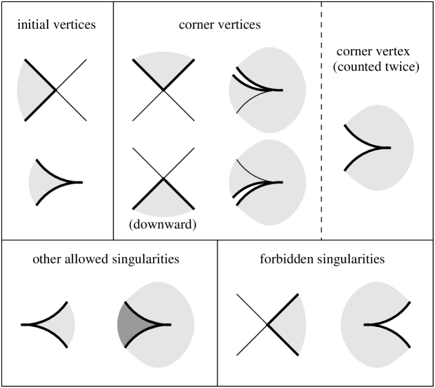
Figure 5. Possible singularities in an admissible map, and their classification. The shaded area is the image of the map restricted to a neighborhood of the singularity; the heavy line indicates the image of the boundary of $D^{2}$. In two of the diagrams, the heavy line has been shifted off of itself for clarity. The diagram with heavy shading indicates that the image overlaps itself.

Definition 2.5.

An admissible map on $Y$ is an immersion from the two-disk $D^{2}$ to $\mathbb{R}^{2}$ which maps the boundary of $D^{2}$ into the knot projection $Y$, and which satisfies the following properties: the map is smooth except possibly at vertices and left cusps; the image of the map near any singularity looks locally like one of the diagrams in Figure 5, excepting the two forbidden ones; and, in the notation of Figure 5, there is precisely one initial vertex.

The singularities of an admissible map thus consist of one initial vertex, a number of corner vertices (possibly including some right cusps counted twice), and some other singularities which we will ignore. One type of corner vertex, the “downward” corner vertex as labelled in Figure 5, will be important shortly in determining signs.

The possible singularities depicted in Figure 5 are all derived by considering the resolution of $Y$, but it is not immediately obvious why the two forbidden singularities should be disallowed. To justify this, call a point $p$ in the domain of an admissible map, and its image under the map, locally rightmost if $p$ attains a local maximum for the $x$ coordinate of its image. Any locally rightmost point in the image of an admissible map must be the unique initial vertex of the map: this point must be a node or a right cusp, which cannot be a negative corner vertex (cf. Figure 5). In particular, there must be a unique locally rightmost point in the image. Of the two forbidden singularities from Figure 5, the left one is disallowed because the initial vertex is not rightmost, and the right one because there would be two locally rightmost points.

To each diffeomorphism class of admissible maps on $Y$, we will now associate a monomial in $\mathbb{Z}[t,t^{-1}]\langle{a_{1},\ldots,a_{n}}\rangle$. Let $f$ be a representative of a diffeomorphism class, and suppose that $f$ has corner vertices at $a_{j_{1}},\ldots,a_{j_{\ell}}$, counted twice where necessary, in counterclockwise order around the boundary of $D^{2}$, starting just after the initial vertex, and ending just before reaching the initial vertex again. Then the monomial associated to $f$, and by extension to the diffeomorphism class of $f$, is

$$\alpha(f)=(\mbox{sgn }f)\,t^{-n(f)}a_{j_{1}}\cdots a_{j_{\ell}},$$

where $(\mbox{sgn }f)$ is the parity ($+1$ for even, $-1$ for odd) of the number of downward corner vertices of $f$ of even degree, and the winding number $n(f)$ is defined below.

The image $f(\partial D^{2})$, oriented counterclockwise, lifts to a collection of oriented paths in the knot $K$. If $a_{i}$ is the initial vertex of $f$, then the lift of $f(\partial D^{2})$, along with the lifts of the capping paths $\gamma_{i}$, $-\gamma_{j_{1}},\ldots,-\gamma_{j_{\ell}}$, form a closed cycle in $K$. We then set $n(f)$ to be the winding number of this cycle around $K$, with respect to the orientation of $K$.

Definition 2.6.

Given a generator $a_{i}$, we define

$$\partial a_{i}=\begin{cases}\sum\alpha(f)&\text{if $a_{i}$ is a crossing}\\ 1+\sum\alpha(f)&\text{if $a_{i}$ is a right cusp oriented upwards}\\ t^{-1}+\sum\alpha(f)&\text{if $a_{i}$ is a right cusp oriented downwards,}\end{cases}$$

where the sum is over all diffeomorphism classes of admissible maps $f$ with initial vertex at $a_{i}$. We extend the differential to the algebra $A$ by setting $\partial(\mathbb{Z}[t,t^{-1}])=0$ and imposing the signed Leibniz rule $\partial(vw)=(\partial v)w+(\mbox{sgn }v)v(\partial w)$.

A few remarks are in order. The power of $t$ in the definition of the monomial $\alpha(f)$ has been translated directly from the corresponding definition in [7]. It is easy to check that the signs also correspond to the signs in [7], after we replace $a_{i}$ by $-a_{i}$ for each $a_{i}$ which is “right-pointing”; that is, near which the knot is locally oriented from left to right for both strands.

Definition 2.6 depends on a choice of orientation of $K$. For an unoriented knot, we may similarly define the differential without the powers of $t$; the DGA is then an algebra over $\mathbb{Z}$ graded over $\mathbb{Z}/(2r(K))$, still a lifting of Chekanov’s original DGA over $\mathbb{Z}/2$.

As a final remark, if $K$ is a stabilization, i.e., contains a zigzag (see, e.g., [6]), then it is easy to see that there is an $a_{i}$ such that $\partial a_{i}=1$ or $\partial a_{i}=t^{-1}$. In this case, $\partial(a_{j}-a_{i}\partial a_{j})=0$ or $\partial(a_{j}-ta_{i}\partial a_{j})=0$ for all $j$, and the DGA collapses modulo tame isomorphisms (see Section 2.4). This was first noted in [1, §11.2].

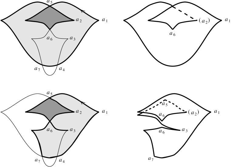
Figure 6. The admissible maps which correspond to the terms $a_{6}$ (top) and $t^{3}a_{6}a_{5}a_{3}a_{6}a_{7}$ (bottom) in $\partial a_{1}$, for the front from Figure 4. The heavy lines indicate the image of the boundary of $D^{2}$; the heavy shading indicates where the images overlap themselves. For clarity, the images of the maps are redrawn to the right.

For the front in Figure 4, we may compute (somewhat laboriously) that

$$\partial a_{1} = 1+a_{6}-t^{2}a_{6}a_{4}a_{6}a_{7}-t^{2}(1-ta_{6}a_{5})a_{3}a_{6}a_{7}+ta_{6}a_{2}(1-ta_{6}-t^{2}a_{7}a_{4}a_{6})a_{7}$$

$$\partial a_{2} = 1-ta_{5}a_{6}$$

$$\partial a_{3} = t^{-1}-a_{6}-ta_{6}a_{7}a_{4}$$

$$\partial a_{4} = \partial a_{5}=\partial a_{6}=\partial a_{7}=0.$$

See Figure 6 for a depiction of two of the admissible maps counted in $\partial a_{1}$.

To illustrate the calculation of the sign and power of $t$ associated to an admissible map, consider the term $t^{3}a_{6}a_{5}a_{3}a_{6}a_{7}$ in $\partial a_{1}$ above. The sign of this term is $(-\mbox{sgn }a_{5})(-\mbox{sgn }a_{6})=+1$. To calculate the power of $t$, we count, with orientation, the number of times the cycle corresponding to this map passes through $a_{1}$. The boundary of the immersed disk passes through $a_{1}$, contributing $1$; $\gamma_{1}$ trivially does not pass through $a_{1}$, contributing $0$; and $-\gamma_{3},-\gamma_{6},-\gamma_{7}$ pass through $a_{1}$, while $-\gamma_{5}$ does not, contributing a total of $-4$. It follows that the power of $t$ is $t^{-(1+0-4)}=t^{3}$.

2.3. Simple fronts

Since the behavior of an admissible map near a right cusp can be complicated, our formulation of the differential algebra may seem no easier to compute than Chekanov’s. There is, however, one class of fronts for which the differential is particularly easy to compute.

Definition 2.7.

A front is simple if it is smoothly isotopic to a front all of whose right cusps have the same $x$ coordinate.

Any front can be Legendrian-isotoped to a simple front: “push” all of the right cusps to the right until they share the same $x$ coordinate. (In the terminology of Figure 1, a series of IIb moves can turn any front into a simple front.)

For a simple front, the boundary of any admissible map must begin at a node or right cusp (the initial vertex), travel leftwards to a left cusp, and then travel rightwards again to the initial vertex. Outside of the initial vertex and the left cusp, the boundary can only have very specific corner vertices: each corner vertex must be a crossing, and, in a neighborhood of each of these nodes, the image of the map must only occupy one of the four regions surrounding the crossing. In particular, the map is an embedding, not just an immersion.

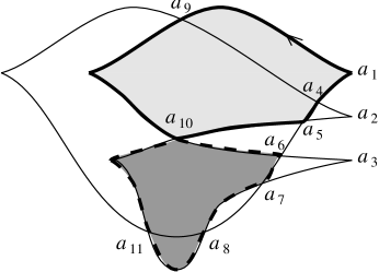
Figure 7. A simple-front version of the front from Figure 4, with two admissible maps drawn. The top shaded region corresponds to the term $ta_{10}a_{5}$ in $\partial a_{1}$; the bottom shaded region corresponds to the term $-ta_{10}a_{7}$ in $\partial a_{6}$.

Example 2.8.

It is easy to calculate the differential for the simple-front version of the figure eight knot given in Figure 7:

$$\begin{array}[]{rclcrcl}\partial a_{1}&=&1+a_{6}+ta_{10}a_{5}&&\partial a_{4}&=&t^{-1}+a_{8}a_{7}-a_{9}a_{6}-ta_{9}a_{10}a_{5}\\ \partial a_{2}&=&1-ta_{9}a_{10}&&\partial a_{5}&=&a_{7}+a_{11}+ta_{11}a_{8}a_{7}\\ \partial a_{3}&=&t^{-1}-a_{10}-ta_{10}a_{11}a_{8}&&\partial a_{6}&=&-ta_{10}a_{7}-ta_{10}a_{11}-t^{2}a_{10}a_{11}a_{8}a_{7}\\ \lx@intercol\hfil\partial a_{7}=\partial a_{8}=\partial a_{9}=\partial a_{10}=\partial a_{11}=0.\hfil\lx@intercol\end{array}$$

For the signs, note that $a_{1},a_{2},a_{3},a_{4},$ and $a_{8}$ have degree 1, $a_{7}$ and $a_{11}$ have degree $-1$, and the other vertices have degree 0; for the powers of $t$, note that $\gamma_{3}$, $\gamma_{4}$, $\gamma_{5}$, $\gamma_{6}$, $\gamma_{7}$, $\gamma_{10}$, and $\gamma_{11}$ pass through $a_{1}$, while the other capping paths do not.

2.4. Properties of the DGA

In this section, we summarize the properties of the Chekanov-Eliashberg DGA. These results were originally proven over $\mathbb{Z}/2$ in [1], and then extended over $\mathbb{Z}[t,t^{-1}]$ in [7]. Proofs can be found in [7] in the Lagrangian-projection setup, or in [12] in the front-projection setup.

Proposition 2.9 ([1],[7]).

For the DGA associated to a Legendrian knot, $\partial$ lowers degree by $1$.

Proposition 2.10 ([1],[7]).

For the DGA associated to a Legendrian knot, $\partial^{2}=0$.

To state the invariance result for the DGA, we need to recall several definitions from [1] or [7].

An (algebra) automorphism of a graded free algebra $\mathbb{Z}[t,t^{-1}]\langle{a_{1},\ldots,a_{n}}\rangle$ is elementary if it preserves grading and sends some $a_{i}$ to $a_{i}+v$, where $v$ does not involve $a_{i}$, and fixes the other generators $a_{j},j\neq i$. A tame automorphism of $\mathbb{Z}[t,t^{-1}]\langle{a_{1},\ldots,a_{n}}\rangle$ is any composition of elementary automorphisms; a tame isomorphism between two free algebras $\mathbb{Z}[t,t^{-1}]\langle{a_{1},\ldots,a_{n}}\rangle$ and $\mathbb{Z}[t,t^{-1}]\langle{b_{1},\ldots,b_{n}}\rangle$ is a grading-preserving composition of a tame automorphism and the map sending $a_{i}$ to $b_{i}$ for all $i$. Two DGAs are then tamely isomorphic if there is a tame isomorphism between them which maps the differential on one to the differential on the other.

Let $E$ be a DGA with generators $e_{1}$ and $e_{2}$, such that $\partial e_{1}=\pm e_{2}$, $\partial e_{2}=0$, both $e_{1}$ and $e_{2}$ have pure degree, and $\deg e_{1}=\deg e_{2}+1$. Then an algebraic stabilization of a DGA $(A=\mathbb{Z}[t,t^{-1}]\langle{a_{1},\ldots,a_{n}}\rangle,\partial)$ is a graded coproduct

$$(S(A),\partial)=(A,\partial)\amalg(E,\partial)=(\mathbb{Z}[t,t^{-1}]\langle{a_{1},\ldots,a_{n},e_{1},e_{2}}\rangle,\partial),$$

with differential and grading induced from $A$ and $E$. Finally, two DGAs are equivalent if they are tamely isomorphic after some (possibly different) number of (possibly different) algebraic stabilizations of each.

We can now state the main invariance result.

Theorem 2.11 ([1],[7]).

Fronts of Legendrian-isotopic knots have equivalent DGAs.

Corollary 2.12 ([1],[7]).

The graded homology of the DGA associated to a Legendrian knot is invariant under Legendrian isotopy.

2.5. The DGA for fronts of links

In this section, we describe the modifications of the definition of the Chekanov-Eliashberg DGA necessary for Legendrian links in standard contact $\mathbb{R}^{3}$. Here the DGA has an infinite family of gradings, as opposed to one, and is defined over a ring more complicated than $\mathbb{Z}[t,t^{-1}]$. The DGA for links also includes some information not found for knots.

Let $L$ be an oriented Legendrian link, with components $L_{1},\ldots,L_{k}$; in this section, for ease of notation, we will also use $L,L_{1},\ldots,L_{k}$ to denote the corresponding front projections. Chekanov’s original definition [1] of the DGA for $L$ gives an algebra over $\mathbb{Z}/2$ graded over $\mathbb{Z}/(2r(L))$, where $r(L)=\gcd(r(L_{1}),\ldots,r(L_{k}))$; we will extend this to an algebra over $\mathbb{Z}[t_{1},t_{1}^{-1},\ldots,t_{k},t_{k}^{-1}]$ graded over $\mathbb{Z}$, and our set of gradings will be more refined than in [1]. We will also discuss an additional structure on the DGA introduced by K. Michatchev [11].

As in Section 2.2, let $a_{1},\ldots,a_{n}$ be the vertices (crossings and right cusps) of $L$. We associate to $L$ the algebra

$$A=\mathbb{Z}[t_{1},t_{1}^{-1},\ldots,t_{k},t_{k}^{-1}]\langle a_{1},\ldots,a_{n}\rangle,$$

with differential and grading to be defined below.

For each crossing $a_{i}$, let $N_{u}(a_{i})$ and $N_{l}(a_{i})$ denote neighborhoods of $a_{i}$ on the two strands intersecting at $a_{i}$, so that the slope of $N_{l}(a_{i})$ is greater than the slope of $N_{u}(a_{i})$, i.e., $N_{u}(a_{i})$ is lower than $N_{l}(a_{i})$ in $y$ coordinate. If $a_{i}$ is a right cusp, define $N_{u}(a_{i})=N_{l}(a_{i})$ to be a neighborhood of $a_{i}$ in $L$. For any vertex $a_{i}$, we may then define two numbers $u(a_{i})$ and $l(a_{i})$, the indices of the link components containing $N_{u}(a_{i})$ and $N_{l}(a_{i})$, respectively.

For each $j=1,\ldots,k$, fix a base point $p_{j}$ on $L_{j}$, away from the singularities of $L$, so that $L_{j}$ is oriented from left to right in a neighborhood of $p_{j}$. To a crossing $a_{i}$, we associate two capping paths $\gamma^{u}_{i}$ and $\gamma^{l}_{i}$: $\gamma^{u}_{i}$ is the path beginning at $p_{u(a_{i})}$ and following $L_{u(a_{i})}$ in the direction of its orientation until $a_{i}$ is reached through $N_{u}(a_{i})$; $\gamma^{l}_{i}$ is the analogous path in $L_{l(a_{i})}$ beginning at $p_{l(a_{i})}$ and ending at $a_{i}$ through $N_{l}(a_{i})$. (If $u(a_{i})=l(a_{i})$, then one of $\gamma^{u}_{i}$ and $\gamma^{l}_{i}$ will contain the other.) Note that, by this definition, when $a_{i}$ is a right cusp, $\gamma^{u}_{i}$ and $\gamma^{l}_{i}$ are both the path beginning at $p_{u(a_{i})}=p_{l(a_{i})}$ and ending at $a_{i}$.

Definition 2.13.

For $(\rho_{1},\ldots,\rho_{k-1})\in\mathbb{Z}^{k-1}$, we may define a $\mathbb{Z}$ grading on $A$ by

$$\deg a_{i}=\begin{cases}1&\text{if $a_{i}$ is a right cusp}\\ c(\gamma^{u}_{i})-c(\gamma^{l}_{i})+2\rho_{u(a_{i})}-2\rho_{l(a_{i})}&\text{if $a_{i}$ is a crossing,}\end{cases}$$

where we set $\rho_{k}=0$. We will only consider gradings on $A$ obtained in this way.

The set of gradings on $A$ is then indexed by $\mathbb{Z}^{k-1}$. (In particular, a knot has precisely one grading, the one given in Section 2.2.) Our motivation for including precisely this set of gradings is given by the following easily proven observation.

Lemma 2.14.

The collection of possible gradings on $A$ is independent of the choices of the points $p_{j}$.

If $a_{i}$ is contained entirely in component $L_{j}$, then the degree of $a_{i}$ may differ from how we defined it in Definition 2.4 with $L_{j}$ a knot by itself. It is easy to calculate that the difference between the two degrees will always be either $0$ or $2r(L_{j})$.

We may define the sign function on vertices, as usual, by $\mbox{sgn }a_{i}=(-1)^{\deg a_{i}}$. This is well-defined and independent of the choice of grading: $\mbox{sgn }a_{i}=-1$ if $a_{i}$ is a right cusp; $\mbox{sgn }a_{i}=1$ if $a_{i}$ is a crossing with both strands pointed in the same direction (either both to the left or both to the right); and $\mbox{sgn }a_{i}=-1$ if $a_{i}$ is a crossing with strands pointed in opposite directions. Note that $tb(L)=\sum_{i=1}^{n}\mbox{sgn }a_{i}$.

We may still define the differential of a generator $a_{i}$ as in Definition 2.6, but we must now redefine $\alpha(f)$ for an admissible map $f$. Suppose that $f$ has initial vertex $a_{i}$ and corner vertices $a_{i_{1}},\ldots,a_{i_{m}}$. Then the lift of $f(\partial D^{2})$ to $L$, together with the lifts of $\gamma^{u}_{i},$ $-\gamma^{u}_{i_{1}},\ldots,-\gamma^{u}_{i_{m}}$, $-\gamma^{l}_{i},$ $\gamma^{l}_{i_{1}},\ldots,\gamma^{l}_{i_{m}},$ form a closed cycle in $L$. Let the winding number of this cycle around component $L_{j}$ be $n_{j}(f)$. Also, define $\mbox{sgn }f$, as before, to be the parity of the number of downward corner vertices of $f$ with positive sign.

We now set

$$\alpha(f)=(\mbox{sgn }f)\,t_{1}^{-n_{1}(f)}\cdots t_{k}^{-n_{k}(f)}a_{i_{1}}\cdots a_{i_{m}}.$$

The differential $\partial$ can then be defined on $A$ essentially as in Definition 2.6, except that we now have $\partial(\mathbb{Z}[t_{1},t_{1}^{-1},\ldots,t_{k},t_{k}^{-1}])=0$, and

$$\partial a_{i}=\begin{cases}\sum\alpha(f)&\text{if $a_{i}$ is a crossing}\\ 1+\sum\alpha(f)&\text{if $a_{i}$ is a right cusp.}\end{cases}$$

Note that the signed Leibniz rule does not depend on the choice of base points $p_{j}$, since the signs $(\mbox{sgn }a_{i})$ are independent of this choice. Also, because of a different choice of capping paths, we always add $1$ to a right cusp; cf. Definition 2.6.

In practice, there is a simple way to calculate $n_{j}(f)$: it is the signed number of times $f(\partial D^{2})$ crosses $p_{j}$. Indeed, the winding number of the appropriate cycle around $L_{j}$ is the signed number of times that it crosses a point on $L_{j}$ just to the left of $p_{j}$. No capping path $\gamma_{i}^{u}$ or $\gamma_{i}^{l}$, however, crosses this point. Hence $n_{j}(f)$ counts the number of times $f(\partial D^{2})$ crosses a point just to the left of $p_{j}$; we could just as well consider $p_{j}$ instead of this point.

We next examine the effect of changing the base points $p_{j}$ on the differential $\partial$. Consider another set of base points $\tilde{p}_{j}$, giving rise to capping paths $\tilde{\gamma}^{u}_{i},\tilde{\gamma}^{l}_{i}$, and let $\xi_{j}$ be the oriented path in $L_{j}$ from $p_{j}^{\prime}$ to $p_{j}$. Then

$$\tilde{\gamma}^{u}_{i}-\gamma^{u}_{i}=\begin{cases}\xi_{u(a_{i})},&N_{u}(a_{i})\subset\xi_{u(a_{i})}\\ \xi_{u(a_{i})}-L_{u(a_{i})},&N_{u}(a_{i})\not\subset\xi_{u(a_{i})},\end{cases}$$

and similarly for $\tilde{\gamma}^{l}_{i}-\gamma^{l}_{i}$. We conclude the following result.

Lemma 2.15.

The differential on $A$, calculated with base points $\tilde{p}_{j}$, is related to the differential calculated with $p_{j}$, by intertwining with the following automorphism on $A$:

$$a_{i}\mapsto\begin{cases}a_{i},&\text{$N_{u}(a_{i})\subset\xi_{u(a_{i})}$ and $N_{l}(a_{i})\subset\xi_{l(a_{i})}$}\\ t_{l(a_{i})}^{-1}a_{i},&\text{$N_{u}(a_{i})\subset\xi_{u(a_{i})}$ and $N_{l}(a_{i})\not\subset\xi_{l(a_{i})}$}\\ t_{u(a_{i})}a_{i},&\text{$N_{u}(a_{i})\not\subset\xi_{u(a_{i})}$ and $N_{l}(a_{i})\subset\xi_{l(a_{i})}$}\\ t_{u(a_{i})}t_{l(a_{i})}^{-1}a_{i},&\text{$N_{u}(a_{i})\not\subset\xi_{u(a_{i})}$ and $N_{l}(a_{i})\not\subset\xi_{l(a_{i})}$.}\end{cases}$$

Figure 8. An oriented link $L$ with components $L_{1}$, $L_{2}$, and $L_{3}$, with corresponding base points $p_{1}$, $p_{2}$, and $p_{3}$ marked but not labelled.

For example, consider the link $L$ in Figure 8, with base points as shown. To give a grading to the DGA on $L$, choose $(\rho_{1},\rho_{2})\in\mathbb{Z}^{2}$. The degrees of generators are as follows:

$$\deg a_{1} =1 \qquad\deg a_{4} =1+2\rho_{2}-2\rho_{1} \qquad\deg a_{7} =-1+2\rho_{1}$$

$$\deg a_{2} =1 \deg a_{5} =1-2\rho_{2} \deg a_{8} =-1+2\rho_{1}-2\rho_{2}$$

$$\deg a_{3} =1 \deg a_{6} =1-2\rho_{1} \deg a_{9} =-1+2\rho_{2}.$$

The differential $\partial$ is then given by

$$\partial a_{1} =1+t_{1}+t_{1}t_{2}^{-1}a_{8}a_{4}+t_{1}t_{3}^{-1}a_{7}a_{6} \qquad\partial a_{4} =t_{2}t_{3}^{-1}a_{9}a_{6} \qquad\partial a_{7} =a_{8}a_{9}$$

$$\partial a_{2} =1+t_{2}+t_{2}t_{3}^{-1}a_{9}a_{5}+a_{4}a_{8} \partial a_{5} =a_{6}a_{8} \partial a_{8} =0$$

$$\partial a_{3} =1+t_{3}+a_{5}a_{9}+a_{6}a_{7} \partial a_{6} =0 \partial a_{9} =0.$$

We can now state several properties of the link DGA, the analogues of the results for knots in Section 2.4.

Proposition 2.16.

If $(A,\partial)$ is a DGA associated to the link $L$, then $\partial^{2}=0$, and $\partial$ lowers degree by $1$ for any of the gradings of $A$.

The main invariance result requires a slight tweaking of the definitions. Define elementary and tame automorphisms as in Section 2.4; now, however, let a tame isomorphism between algebras generated by $a_{1},\ldots,a_{n}$ and $b_{1},\ldots,b_{n}$ be a grading-preserving composition of a tame automorphism and a map sending $a_{i}$ to $\left(\prod_{m=1}^{k}t_{m}^{\nu_{k,m}}\right)b_{i}$, for any set of integers $\{\nu_{k,m}\}$. (This definition is necessitated by Lemma 2.15.) Define algebraic stabilization and equivalence as before.

Proposition 2.17.

If $L$ and $L^{\prime}$ are Legendrian-isotopic oriented links, then for any grading of the DGA for $L$, there is a grading of the DGA for $L^{\prime}$ so that the two DGAs are equivalent.

The proofs of Propositions 2.16 and 2.17 will be omitted here, as they are simply variants on the proofs of Propositions 2.9 and 2.10 and Theorem 2.11; see [1] or [12].

Our set of gradings for $A$ is more restrictive than the set of “admissible gradings” postulated in [1]. To see this, we first translate our criteria for gradings to the Lagrangian-projection picture, and then compare with Chekanov’s original criteria.

Consider a Legendrian link $L$ with components $L_{1},\ldots,L_{k}$. By perturbing $L$ slightly, we may assume that the crossings of $\pi_{xy}(L)$ are orthogonal, where $\pi_{xy}$ is the projection map $(x,y,z)\mapsto(x,y)$; as usual, label these crossings $a_{1},\ldots,a_{n}$. Choose neighborhoods $N_{u}(a_{i})$ and $N_{l}(a_{i})$ in $L$ of the two points mapping to $a_{i}$ under $\pi_{xy}$, so that $N_{u}(a_{i})$ lies above $N_{l}(a_{i})$ in $z$ coordinate, and let $u(a_{i})$ and $l(a_{i})$ be the indices of the link components on which these neighborhoods lie.

For each $j$, choose a point $p_{j}$ on $L_{j}$, and let $\theta_{j}$ be an angle, measured counterclockwise, from the positive $x$ axis to the oriented tangent to $L_{j}$ at $p_{j}$; note that $\theta_{j}$ is only well-defined up to multiples of $2\pi$. Let $r_{u}(a_{i})$ be the counterclockwise rotation number (the number of revolutions made) for the path in $\pi(L_{u(a_{i})})$ beginning at $p_{u(a_{i})}$ and following the orientation of $L_{u(a_{i})}$ until $a_{i}$ is reached via $N_{u}(a_{i})$; similarly define $r_{l}(a_{i})$. Then the gradings for the DGA of $L$ are given by choosing $(\rho_{1},\ldots,\rho_{k-1})\in\mathbb{Z}^{k-1}$ and setting

$$\deg a_{i}=2(r_{l}(a_{i})-r_{u}(a_{i}))+(\theta_{l(a_{i})}-\theta_{u(a_{i})})/\pi+2\rho_{u(a_{i})}-2\rho_{l(a_{i})}-1/2.$$

By comparison, the allowed degrees in [1] are given by

$$\deg a_{i}=2(r_{l}(a_{i})-r_{u}(a_{i}))+(\theta_{l(a_{i})}-\theta_{u(a_{i})})/\pi+\rho_{u(a_{i})}-\rho_{l(a_{i})}-1/2.$$

The difference arises from the fact that Chekanov never uses the orientations of the link components; this forces $\theta_{l(a_{i})}$ and $\theta_{r(a_{i})}$ to be well-defined only up to integer multiples of $\pi$, rather than $2\pi$.

We now discuss an additional structure on the DGA for a link $L$, inspired by [11]. More precisely, we will describe a variant of the relative homotopy splitting from [11]; our variant will split something which is essentially a submodule of the DGA into $k^{2}$ pieces which are invariant under Legendrian isotopy.

Definition 2.18.

For $j_{1}\neq j_{2}$ between $1$ and $k$, inclusive, define $\Gamma_{j_{1}j_{2}}$ to be the module over $\mathbb{Z}[t_{1},t_{1}^{-1},\ldots,t_{k},t_{k}^{-1}]$ generated by words of the form $a_{i_{1}}\cdots a_{i_{m}}$, with $u(a_{i_{1}})=j_{1},$ $l(a_{i_{m}})=j_{2}$, and $u(a_{i_{p+1}})=l(a_{i_{p}})$ for $1\leq p\leq m-1$. If $j_{1}=j_{2}=j$, then let $\Gamma_{j_{1}j_{2}}$ be the module generated by such words, along with an indeterminate $e_{j}$. Finally, let $\Gamma=\oplus\Gamma_{j_{1}j_{2}}$.

The indeterminates $e_{j}$ will replace the $1$ terms in the definition of $\partial$; see below. Note that $a_{i}\in\Gamma_{u(a_{i})l(a_{i})}$. Although $\Gamma$ itself is not an algebra, we have the usual multiplication map $\Gamma_{j_{1}j_{2}}\times\Gamma_{j_{2}j_{3}}\rightarrow\Gamma_{j_{1}j_{3}}$, given on generators by concatenation, once we stipulate that the $e_{j}$’s act as the identity.

Our introduction of $\Gamma$ is motivated by the fact that $\partial a_{i}$ is essentially in $\Gamma_{u(a_{i})l(a_{i})}$ for all $i$. Define $\partial^{\prime}a_{i}$ as follows: if $u(a_{i})\neq l(a_{i})$, then $\partial^{\prime}a_{i}=\partial a_{i}$; if $u(a_{i})=l(a_{i})$, then $\partial^{\prime}a_{i}$ is $\partial a_{i}$, except that we replace any $1$ or $2$ term in $\partial a_{i}$ by $e_{u(a_{i})}$ or $2e_{u(a_{i})}$. (It is easy to see that these are the only possible terms in $\partial a_{i}$ which involve only the $t_{j}$’s and no $a_{m}$’s.)

Lemma 2.19.

$\partial^{\prime}a_{i}\in\Gamma_{u(a_{i})l(a_{i})}$ for all $i$.

Proof.

For a term in $\partial a_{i}$ of the form $a_{i_{1}}\ldots a_{i_{k}}$, where we exclude powers of $t_{j}$’s, we wish to prove that $u(a_{i_{1}})=u(a_{i})$, $l(a_{i_{k}})=l(a_{i})$, and $u(a_{i_{p+1}})=l(a_{i_{p}})$ for all $p$. Consider the boundary of the map which gives the term $a_{i_{1}}\ldots a_{i_{k}}$. By definition, the portion of this boundary connecting $a_{i_{p}}$ to $a_{i_{p+1}}$ belongs to link component $l(a_{i_{p}})$ on one hand, and $u(a_{i_{p+1}})$ on the other. We similarly find that $u(a_{i_{1}})=u(a_{i})$ and $l(a_{i_{k}})=l(a_{i})$. ∎

Definition 2.20.

The differential link module of $L$ is $(\Gamma,\partial^{\prime})$, where we have defined $\partial^{\prime}a_{i}$ above, and we extend $\partial^{\prime}$ to $\Gamma$ by applying the signed Leibniz rule and setting $\partial^{\prime}e_{j}=0$ for all $j$. A grading for $\Gamma$ is one inherited from the DGA of $L$, with $\deg e_{j}=0$ for all $j$.

We may define (grading-preserving) elementary and tame automorphisms and tame isomorphisms for differential link modules as for DGAs, with the additional stipulation that all maps must preserve the link module structure by preserving $\Gamma_{j_{1}j_{2}}$ for all $j_{1},j_{2}$. Similarly, we may define an algebraic stabilization of a differential link module, with the additional stipulation that the two added generators both belong to the same $\Gamma_{j_{1}j_{2}}$. As usual, we then define two differential link modules to be equivalent if they are tamely isomorphic after some number of algebraic stabilizations. We omit the proof of the following result, which again is simply a variant on the proof of the corresponding result for knots.

Proposition 2.21.

If $L$ and $L^{\prime}$ are Legendrian-isotopic oriented links, then for any grading of the differential link module for $L$, there is a grading of the differential link module for $L^{\prime}$ so that the two are equivalent.

In this paper, we will not use the full strength of the differential link module. We will, however, apply first-order Poincaré-Chekanov polynomials derived from the differential link module; we now describe these polynomials, first mentioned in [11]. For the definition of augmentations for knots, and background on Poincaré-Chekanov polynomials, please refer to [1] or Section 3.2.

Assume that $r(L_{1})=\cdots=r(L_{k})=0$, and let $\Gamma$ be the differential link module for $L$, with some fixed grading. We consider the DGAs for $L$ and $L_{1},\ldots,L_{k}$ over $\mathbb{Z}/2$; that is, set $t_{j}=1$ for all $j$, and reduce modulo 2.

Definition 2.22.

Suppose that, when considered alone as a knot, the DGA for each of $L_{1},\ldots,L_{k}$ has an augmentation $\varepsilon_{1},\ldots,\varepsilon_{k}$. Extend these augmentations to all vertices $a_{i}$ of $L$ by setting

$$\varepsilon(a_{i})=\begin{cases}\varepsilon_{u(a_{i})}(a_{i})&\text{if $u(a_{i})=l(a_{i})$}\\ 0&\text{otherwise.}\end{cases}$$

We define an augmentation of $L$ to be any function $\varepsilon$ obtained in this way.

An augmentation $\varepsilon$, as usual, gives rise to a first-order Poincaré-Chekanov polynomial $P^{\varepsilon,1}(\lambda)$; we may say, a bit imprecisely, that this polynomial splits into $k^{2}$ polynomials $P^{\varepsilon,1}_{j_{1}j_{2}}(\lambda)$, corresponding to the pieces in $\Gamma_{j_{1}j_{2}}$.

The polynomials $P^{\varepsilon,1}_{jj}(\lambda)$ are precisely the polynomials $P^{\varepsilon_{j},1}(\lambda)$ for each individual link component $L_{j}$. For practical purposes, we can define $P^{\varepsilon,1}_{j_{1}j_{2}}(\lambda)$ for $j_{1}\neq j_{2}$ as follows. For $a_{i}\in\Gamma_{j_{1}j_{2}}$, define $\partial_{\varepsilon}^{(1)}a_{i}$ to be the image of $\partial a_{i}$ under the following operation: discard all terms in $\partial a_{i}$ containing more than one $a_{m}$ with $u(a_{m})\neq l(a_{m})$, and replace each $a_{m}$ in $\partial a_{i}$ by $\varepsilon(a_{m})$ whenever $u(a_{m})=l(a_{m})$. If we write $V_{j_{1}j_{2}}$ as the vector space over $\mathbb{Z}/2$ generated by $\{a_{i}\in\Gamma_{j_{1}j_{2}}\}$, then $\partial_{\varepsilon}^{(1)}$ preserves $V_{j_{1}j_{2}}$ and $\left(\partial_{\varepsilon}^{(1)}\right)^{2}=0$. We may then set $P^{\varepsilon,1}_{j_{1}j_{2}}(\lambda)$ to be the Poincaré polynomial of $\partial_{\varepsilon}^{(1)}$ on $V_{j_{1}j_{2}}$, i.e., the polynomial in $\lambda$ whose $\lambda^{i}$ coefficient is the dimension of the $i$-th graded piece of $(\ker\partial_{\varepsilon}^{(1)})/({\rm im}\partial_{\varepsilon}^{(1)})$.

We may also define higher-order Poincaré-Chekanov polynomials $P^{\varepsilon,n}_{j_{1}j_{2}}(\lambda)$ by examining the action of $\partial^{\prime}$ on $\Gamma_{j_{1}j_{2}}$, but we will not need these here.

The following result, which follows directly from Proposition 2.21 and Chekanov’s corresponding result from [1], will be used in Section 4.

Theorem 2.23.

Suppose that $L$ and $L^{\prime}$ are Legendrian-isotopic oriented links. Then, for any given grading and augmentation of the DGA for $L$, there is a grading and augmentation of the DGA for $L^{\prime}$ so that the first-order Poincaré-Chekanov polynomials $P^{\varepsilon,1}_{j_{1}j_{2}}$ for $L$ and $L^{\prime}$ are equal for all $j_{1},j_{2}$.

For unoriented links, we simply expand the set of allowed gradings $(\rho_{1},\ldots,\rho_{k-1})$ to allow half-integers, as in [1]. Indeed, a grading of half-integers $(\rho_{1},\ldots,\rho_{k-1})$ corresponds to changing the original orientation of $L$ by either reversing the orientation of $\{L_{j}\,:\,2\rho_{j}~{}\mbox{odd}\}$, or reversing the orientations of $L_{k}$ and $\{L_{j}\,:\,2\rho_{j}~{}\mbox{even}\}$. We deduce this by examining how the capping paths and degrees change when we change the orientation (and hence base point) of one link component $L_{j}$.

For the link from Figure 8, an augmentation is any map with $\varepsilon(a_{i})=0$ for $i\geq 4$. Then $\partial_{\varepsilon}^{(1)}$ is identically zero, and the first-order Poincaré-Chekanov polynomials simply measure the degrees of the $a_{i}$. More precisely, for a choice of grading $(\rho_{1},\rho_{2})\in\mathbb{Z}^{2}$, we have

$$P^{\varepsilon,1}_{11}(\lambda) =\lambda \qquad P^{\varepsilon,1}_{21}(\lambda) =\lambda^{1+2\rho_{2}-2\rho_{1}} \qquad P^{\varepsilon,1}_{31}(\lambda) =\lambda^{1-2\rho_{1}}$$

$$P^{\varepsilon,1}_{12}(\lambda) =\lambda^{-1+2\rho_{1}-2\rho_{2}} \qquad P^{\varepsilon,1}_{22}(\lambda) =\lambda \qquad P^{\varepsilon,1}_{32}(\lambda) =\lambda^{1-2\rho_{2}}$$

$$P^{\varepsilon,1}_{13}(\lambda) =\lambda^{-1+2\rho_{1}} \qquad P^{\varepsilon,1}_{23}(\lambda) =\lambda^{-1+2\rho_{2}} \qquad P^{\varepsilon,1}_{33}(\lambda) =\lambda.$$

3. The characteristic algebra

We would like to use the Chekanov-Eliashberg DGA to distinguish between Legendrian isotopy classes of knots. Unfortunately, it is often hard to tell when two DGAs are equivalent. In particular, the homology of a DGA is generally infinite-dimensional and difficult to grasp; this prevents us from applying Corollary 2.12 directly.

Until now, the only known “computable” Legendrian invariants—that is, nonclassical invariants which can be used in practice to distinguish between Legendrian isotopy classes of knots—were the first-order Poincaré-Chekanov polynomial and its higher-order analogues. However, the Poincaré-Chekanov polynomial is not defined for all Legendrian knots, nor is it necessarily uniquely defined; in addition, as we shall see, there are many nonisotopic knots with the same polynomial. The higher-order polynomials, on the other hand, are difficult to compute, and have not yet been successfully used to distinguish Legendrian knots.

In Section 3.1, we introduce the characteristic algebra, a Legendrian invariant derived from the DGA, which is nontrivial for most, if not all, Legendrian knots with maximal Thurston-Bennequin number. The characteristic algebra encodes the information from at least the first- and second-order Poincaré-Chekanov polynomials, as we explain in Section 3.2. We will demonstrate the efficacy of our invariant, through examples, in Section 4.

Although the results of this section hold for links as well, we will confine our attention to knots for simplicity, except at the end of Section 3.1.

3.1. Definition of the characteristic algebra

The characteristic algebra can be viewed as a close relative of the DGA homology, except that it is easier to handle in general than the homology itself.

Definition 3.1.

Let $(A,\partial)$ be a DGA over $\mathbb{Z}[t,t^{-1}]$, where $A=\mathbb{Z}[t,t^{-1}]\langle{a_{1},\ldots,a_{n}}\rangle$, and let $I$ denote the (two-sided) ideal in $A$ generated by $\{\partial a_{i}\,|\,1\leq i\leq n\}$. The characteristic algebra $\mathcal{C}(A,\partial)$ is defined to be the algebra $A/I$, with grading induced from the grading on $A$.

Definition 3.2.

Two characteristic algebras $A_{1}/I_{1}$ and $A_{2}/I_{2}$ are tamely isomorphic if we can add some number of generators to $A_{1}$ and the same generators to $I_{1}$, and similarly for $A_{2}$ and $I_{2}$, so that there is a tame isomorphism between $A_{1}$ and $A_{2}$ sending $I_{1}$ to $I_{2}$.

In particular, tamely isomorphic characteristic algebras are isomorphic as algebras. Strictly speaking, Definition 3.2 only makes sense if we interpret the characteristic algebra as a pair $(A,I)$ rather than as $A/I$, but we will be sloppy with our notation. Recall that we defined tame isomorphism between free algebras in Section 2.4.

A stabilization of $(A,\partial)$, as defined in Section 2.4, adds two generators $e_{1},e_{2}$ to $A$ and one generator $e_{2}$ to $I$; thus $A/I$ changes by adding one generator $e_{1}$ and no relations.

Definition 3.3.

Two characteristic algebras $A_{1}/I_{1}$ and $A_{2}/I_{2}$ are equivalent if they are tamely isomorphic, after adding a (possibly different) finite number of generators (but no additional relations) to each.

Theorem 3.4.

Legendrian-isotopic knots have equivalent characteristic algebras.

Proof.

Let $(A,\partial)$ be a DGA with $A=\mathbb{Z}[t,t^{-1}]\langle{a_{1},\ldots,a_{n}}\rangle$. Consider an elementary automorphism of $A$ sending $a_{j}$ to $a_{j}+v$, where $v$ does not involve $a_{j}$; since $\partial(a_{j}+v)$ is in $I$, it is easy to see that this automorphism descends to a map on characteristic algebras. We conclude that tamely isomorphic DGAs have tamely isomorphic characteristic algebras. On the other hand, equivalence of characteristic algebras is defined precisely to be preserved under stabilization of DGAs. ∎

In the case of a link, we may also define the characteristic module arising from the differential link module $(\Gamma,\partial^{\prime})$ introduced in Section 2.5. This is the module over $\mathbb{Z}[t_{1},t_{1}^{-1},\ldots,t_{k},t_{k}^{-1}]$ generated by $\Gamma$, modulo the relations

$$v_{1}(\partial^{\prime}a_{i})v_{2}=0\,:\,v_{1}\in\Gamma_{j_{1}j_{2}},a_{i}\in\Gamma_{j_{2}j_{3}},v_{2}\in\Gamma_{j_{3}j_{4}}~{}\text{for some $j_{1},j_{2},j_{3},j_{4}$}.$$

Define equivalence of characteristic modules similarly to equivalence of characteristic algebras, except that replacing a generator $a_{i}$ by $t_{u(a_{i})}^{\pm 1}a_{i}$ or $t_{l(a_{i})}^{\pm 1}a_{i}$ is allowed. Then Legendrian-isotopic links have equivalent characteristic modules. An approach along these lines is used in [11] to distinguish between particular links.

3.2. Relation to the Poincaré-Chekanov polynomial invariants

In this section, we work over $\mathbb{Z}/2$ rather than over $\mathbb{Z}[t,t^{-1}]$; simply set $t=1$ and reduce modulo 2. Thus we consider the DGA $(A,\partial)$ of a Legendrian knot $K$ over $\mathbb{Z}/2$, graded over $\mathbb{Z}/(2r(K))$; let $\mathcal{C}=A/I$ be its characteristic algebra.

We first review the definition of the Poincaré-Chekanov polynomials. The following term is taken from [4].

Definition 3.5.

Let $(A,\partial)$ be a DGA over $\mathbb{Z}/2$. An algebra map $\varepsilon\,:\,A\rightarrow\mathbb{Z}/2$ is an augmentation if $\varepsilon(1)=1$, $\varepsilon\circ\partial=0$, and $\varepsilon$ vanishes for any element in $A$ of nonzero degree.

Given an augmentation $\varepsilon$ of $(A,\partial)$, write $A_{\varepsilon}=\ker\varepsilon$; then $\partial$ maps $(A_{\varepsilon})^{n}$ into itself for all $n$, and thus $\partial$ descends to a map $\partial^{(n)}\,:\,A_{\varepsilon}/A_{\varepsilon}^{n+1}\rightarrow A_{\varepsilon}/A_{\varepsilon}^{n+1}$. We can break $A_{\varepsilon}/A_{\varepsilon}^{n+1}$ into graded pieces $\sum_{i\in\mathbb{Z}/(2r(K))}C_{i}^{(n)}$, where $C_{i}^{(n)}$ denotes the piece of degree $i$. Write $\alpha_{i}^{(n)}=\dim_{\mathbb{Z}/2}\ker(\partial^{(n)}:C_{i}^{(n)}\rightarrow C_{i-1}^{(n)})$ and $\beta_{i}^{(n)}=\dim_{\mathbb{Z}/2}{\rm im}(\partial^{(n)}:C_{i+1}^{(n)}\rightarrow C_{i}^{(n)})$, so that $\alpha_{i}^{(n)}-\beta_{i}^{(n)}$ is the dimension of the $i$-th graded piece of the homology of $\partial^{(n)}$.

Definition 3.6.

The Poincaré-Chekanov polynomial of order $n$ associated to an augmentation $\varepsilon$ of $(A,\partial)$ is $P_{\varepsilon,n}(\lambda)=\sum_{i\in\mathbb{Z}/(2r(K))}\left(\alpha_{i}^{(n)}-\beta_{i}^{(n)}\right)\lambda^{i}$.

Note that augmentations of a DGA do not always exist.

The main result of this section states that we can recover some Poincaré-Chekanov polynomials from the characteristic algebra. To do this, we need one additional bit of information, besides the characteristic algebra.

Definition 3.7.

Let $\gamma_{i}$ be the number of generators of degree $i$ of a DGA $(A,\partial)$ graded over $\mathbb{Z}/(2r(K))$. Then the degree distribution $\gamma\,:\,\mathbb{Z}/(2r(K))\rightarrow\mathbb{Z}_{\geq 0}$ of $A$ is the map $i\mapsto\gamma_{i}$.

Clearly, the degree distribution can be immediately computed from a diagram of $K$ by calculating the degrees of the vertices of $K$.

We are now ready for the main result of this section. Note that the following proposition uses the isomorphism class, not the equivalence class, of the characteristic algebra.

Proposition 3.8.

The set of first- and second-order Poincaré-Chekanov polynomials for all possible augmentations of a DGA $(A,\partial)$ is determined by the isomorphism class of the characteristic algebra $\mathcal{C}$ and the degree distribution of $A$.

Before we can prove Proposition 3.8, we need to establish a few ancillary results. Our starting point is the observation that there is a one-to-one correspondence between augmentations and maximal ideals $\langle a_{1}+c_{1},\ldots,a_{n}+c_{n}\rangle\subset A$ containing $I$ and satisfying $c_{i}=0$ if $\deg a_{i}\neq 0$.

Fix an augmentation $\varepsilon$. We first assume for convenience that $\varepsilon=0$; then $I\subset M$, where $M$ is the maximal ideal $\langle a_{1},\ldots,a_{n}\rangle$. For each $i$, write

$$\partial a_{i}=\partial_{1}a_{i}+\partial_{2}a_{i}+\partial_{3}a_{i},$$

where $\partial_{1}a_{i}$ is linear in the $a_{j}$, $\partial_{2}a_{i}$ is quadratic in the $a_{j}$, and $\partial_{3}a_{i}$ contains terms of third or higher order. The following lemma writes $\partial_{1}$ in a standard form.

Lemma 3.9.

After applying a tame automorphism, we can relabel the $a_{i}$ as $a_{1},\ldots,a_{k},b_{1},\ldots,b_{k}$, $c_{1},\ldots,c_{n-2k}$ for some $k$, so that $\partial_{1}a_{i}=b_{i}$ and $\partial_{1}b_{i}=\partial_{1}c_{i}=0$ for all $i$.

Proof.

For clarity, we first relabel the $a_{i}$ as $\tilde{a}_{i}$. We may assume that the $\tilde{a}_{i}$ are ordered so that $\partial\tilde{a}_{i}$ contains only terms involving $\tilde{a}_{j}$, $j<i$; see [1]. Let $i_{1}$ be the smallest number so that $\partial_{1}\tilde{a}_{i_{1}}\neq 0$. We can write $\partial_{1}\tilde{a}_{i_{1}}=\tilde{a}_{j_{1}}+v_{1}$, where $j_{1}<i_{1}$ and the expression $v_{1}$ does not involve $\tilde{a}_{j_{1}}$. After applying the elementary isomorphism $\tilde{a}_{j_{1}}\mapsto\tilde{a}_{j_{1}}+v_{1}$, we may assume that $v_{1}=0$ and $\partial_{1}\tilde{a}_{i_{1}}=\tilde{a}_{j_{1}}$.

For any $\tilde{a}_{i}$ such that $\partial_{1}\tilde{a}_{i}$ involves $\tilde{a}_{j_{1}}$, replace $\tilde{a}_{i}$ by $\tilde{a}_{i}+\tilde{a}_{i_{1}}$. Then $\partial_{1}\tilde{a}_{i}$ does not involve $\tilde{a}_{j_{1}}$ unless $i=i_{1}$; in addition, no $\partial_{1}\tilde{a}_{i}$ can involve $\tilde{a}_{i_{1}}$, since then $\partial_{1}^{2}\tilde{a}_{i}$ would involve $\tilde{a}_{j_{1}}$. Set $a_{1}=\tilde{a}_{i_{1}}$ and $b_{1}=\tilde{a}_{i_{1}}$; then $\partial_{1}a_{1}=b_{1}$ and $\partial_{1}\tilde{a}_{i}$ does not involve $a_{1}$ or $b_{1}$ for any other $i$.

Repeat this process with the next smallest $\tilde{a}_{i_{2}}$ with $\partial_{1}\tilde{a}_{i_{2}}\neq 0$, and so forth. At the conclusion of this inductive process, we obtain $a_{1},\ldots,a_{k},b_{1},\ldots,b_{k}$ with $\partial_{1}a_{i}=b_{i}$ (and $\partial_{1}b_{i}=0$), and the remaining $\tilde{a}_{i}$ satisfy $\partial_{1}\tilde{a}_{i}=0$; relabel these remaining generators with $c$’s. ∎

Now assume that we have relabelled the generators of $A$ in accordance with Lemma 3.9.

Lemma 3.10.

$\beta_{\ell}^{(1)}$ is the number of $b_{j}$ of degree $\ell$, while $\beta_{\ell}^{(2)}-\beta_{\ell}^{(1)}$ is the dimension of the degree $\ell$ subspace of the vector space generated by

$$\{\partial_{2}b_{i},\partial_{2}c_{i},a_{i}b_{j}+b_{i}a_{j},b_{i}b_{j},b_{i}c_{j},c_{i}b_{j}\},$$

where $i,j$ range over all possible indices.

Proof.

The statement for $\beta_{\ell}^{(1)}$ is obvious. To calculate $\beta_{\ell}^{(2)}-\beta_{\ell}^{(1)}$, note that the image of $\partial^{(2)}$ in $A/A^{3}$ is generated by $\partial a_{i}=b_{i}+\partial_{2}a_{i}$, $\partial b_{i}=\partial_{2}b_{i}$, $\partial c_{i}=\partial_{2}c_{i}$, $\partial(a_{i}a_{j})=a_{i}b_{j}+b_{i}a_{j}$, $\partial(a_{i}b_{j})=b_{i}b_{j}$, $\partial(b_{i}a_{j})=b_{i}b_{j}$, $\partial(a_{i}c_{j})=b_{i}c_{j}$, and $\partial(c_{i}a_{j})=c_{i}b_{j}$. ∎

We wish to write $\beta_{\ell}^{(n)}$ in terms of $\mathcal{C}$, but we first pass through an intermediate step. Let $N^{(n)}$ be the image of $I$ in $M/M^{n+1}$, and let $\delta_{\ell}^{(n)}$ be the dimension of the degree $\ell$ part of $N^{(n)}$. Lemma 3.12 below relates $\beta_{\ell}^{(n)}$ to $\delta_{\ell}^{(n)}$ for $n=1,2$.

Lemma 3.11.

$\delta_{\ell}^{(1)}$ is the number of $b_{i}$ of degree $\ell$, while $\delta_{\ell}^{(2)}-\delta_{\ell}^{(1)}$ is the dimension of the degree $\ell$ subspace of the vector space generated by

$$\{\partial_{2}b_{i},\partial_{2}c_{i},a_{i}b_{j},b_{i}a_{j},b_{i}b_{j},b_{i}c_{j},c_{i}b_{j}\},$$

where $i,j$ range over all possible indices.

Proof.

This follows immediately from the fact that $I$ is generated by $\{\partial a_{i},\partial b_{i},\partial c_{i}\}$. ∎

Lemma 3.12.

$\beta_{\ell}^{(1)}=\delta_{\ell}^{(1)}$ and $\beta_{\ell}^{(2)}=\delta_{\ell}^{(2)}-\sum_{\ell^{\prime}}\delta_{\ell^{\prime}}\delta_{\ell-\ell^{\prime}-1}$.

Proof.

We use Lemmas 3.10 and 3.11. The first equality is obvious. For the second equality, we claim that, for fixed $i$ and $j$, $a_{i}b_{j}$ only appears in conjunction with $b_{i}a_{j}$ in the expressions $\partial_{2}b_{m}$ and $\partial_{2}c_{m}$, for arbitrary $m$. It then follows that $\delta_{\ell}^{(2)}-\beta_{\ell}^{(2)}$ is the number of $a_{i}b_{j}$ of degree $\ell$, which is $\sum_{\ell^{\prime}}\delta_{\ell^{\prime}}\delta_{\ell-\ell^{\prime}-1}$.

To prove the claim, suppose that $\partial_{2}b_{m}$ contains a term $a_{i}b_{j}$. Since $\partial_{2}^{2}b_{m}=0$ and $\partial_{2}(a_{i}b_{j})=b_{i}b_{j}$, there must be another term in $\partial_{2}b_{m}$ which, when we apply $\partial_{2}$, gives $b_{i}b_{j}$; but this term can only be $b_{i}a_{j}$. The same argument obviously holds for $\partial_{2}c_{m}$. ∎

Now let $\varepsilon$ be any augmentation, and let $M_{\varepsilon}=\langle a_{1}+\varepsilon(a_{1}),\ldots,a_{n}+\varepsilon(a_{n})\rangle$ be the corresponding maximal ideal in $A$. If we define $N^{(n)}$ and $\delta_{\ell}^{(n)}$ as above, except with $M$ replaced by $M_{\varepsilon}$, then Lemma 3.12 still holds. We are now ready to prove Proposition 3.8.

Proof of Proposition 3.8.

Note that

$$(M_{\varepsilon}/M_{\varepsilon}^{n+1})/N^{(n)}\cong(M_{\varepsilon}/I)/(M_{\varepsilon}/I)^{n+1};$$

the characteristic algebra $\mathcal{C}=A/I$ and the choice of augmentation $\varepsilon$ determine the right hand side. On the other hand, the dimension of the degree $\ell$ part of $M_{\varepsilon}/M_{\varepsilon}^{n+1}$ is $\gamma_{\ell}$ if $n=1$, and $\gamma_{\ell}+\sum_{\ell^{\prime}}\gamma_{\ell^{\prime}}\gamma_{\ell-\ell^{\prime}}$ if $n=2$. It follows that we can calculate $\{\delta_{\ell}^{(1)}\}$ and $\{\delta_{\ell}^{(2)}\}$ from $\mathcal{C}$, $\varepsilon$, and $\gamma$.

Fix $n=1,2$. By Lemma 3.12, we can then calculate $\{\beta_{\ell}^{(n)}\}$ and hence the Poincaré-Chekanov polynomial

$$P_{\varepsilon,n}(\lambda)=\sum_{\ell}\left((\alpha_{\ell}^{(n)}+\beta_{\ell-1}^{(n)})-\beta_{\ell}^{(n)}-\beta_{\ell-1}^{(n)}\right)\lambda^{\ell}.$$

Letting $\varepsilon$ vary over all possible augmentations yields the proposition. ∎

The situation for higher-order Poincaré-Chekanov polynomials seems more difficult; we tentatively make the following conjecture.

Conjecture 3.13.

The isomorphism class of $\mathcal{C}$ and the degree distribution of $A$ determine the Poincaré-Chekanov polynomials in all orders.

Another set of invariants, similar to the Poincaré-Chekanov polynomials, are obtained by ignoring the grading of the DGA, and considering ungraded augmentations. In this case, the invariants are a set of integers, rather than polynomials, in each order. A proof similar to the one above shows that the first- and second-order ungraded invariants are determined by the characteristic algebra.

In practice, we apply Proposition 3.8 as follows. Given two DGAs, stabilize each with the appropriate number and degrees of stabilizations so that the two resulting DGAs have the same degree distribution. If these new DGAs have isomorphic characteristic algebras, then they have the same first- and second-order Poincaré-Chekanov polynomials (if augmentations exist). If not, then we can often see that their characteristic algebras are not equivalent, and so the original DGAs are not equivalent. Thus calculating characteristic algebras often obviates the need to calculate first- and second-order Poincaré-Chekanov polynomials.

Note that the first-order Poincaré-Chekanov polynomials depend only on the abelianization of $(A,\partial)$; if the procedure described above yields two characteristic algebras whose abelianizations are isomorphic, then the original DGAs have the same first-order Poincaré-Chekanov polynomials. On a related note, empirical evidence leads us to propose the following conjecture, which would yield a new topological knot invariant.

Conjecture 3.14.

For a Legendrian knot $K$ with maximal Thurston-Bennequin number, the equivalence class of the abelianized characteristic algebra of $K$, considered without grading and over $\mathbb{Z}$, depends only on the topological class of $K$.

Here the abelianization is unsigned: $vw=wv$ for all $v,w$.

We can view the abelianization of $\mathcal{C}$ in terms of algebraic geometry. If $\mathcal{C}=(\mathbb{Z}/2)\langle a_{1},\ldots,a_{n}\rangle\,/\,I$, then the abelianization of $\mathcal{C}$ gives rise to a scheme $X$ in $\mathbb{A}^{n}$, affine $n$-space over $\mathbb{Z}/2$. Theorem 3.4 immediately implies the following result.

Corollary 3.15.

The scheme $X$ is a Legendrian-isotopy invariant, up to changes of coordinates and additions of extra coordinates (i.e., we can replace $X\subset\mathbb{A}^{n}$ by $X\times\mathbb{A}\subset\mathbb{A}^{n+1}$).

There is a conjecture about first-order Poincaré-Chekanov polynomials, suggested by Chekanov, which has a nice interpretation in our scheme picture.

Conjecture 3.16 ([1]).

The first-order Poincaré-Chekanov polynomial is independent of the augmentation $\varepsilon$.

Augmentations are simply the $(\mathbb{Z}/2)$-rational points in $X$, graded in the sense that all coordinates corresponding to nonzero-degree $a_{j}$ are zero. It is not hard to see that the first-order Poincaré-Chekanov polynomial at a $(\mathbb{Z}/2)$-rational point $p$ in $X$ is precisely the “graded” codimension in $\mathbb{A}^{n}$ of $T_{p}X$, the tangent space to $X$ at $p$. The following conjecture, which we have verified in many examples, would imply Conjecture 3.16.

Conjecture 3.17.

The scheme $X$ is irreducible and smooth at each $(\mathbb{Z}/2)$-rational point.

4. Applications

In this section, we give several illustrations of the constructions and results from Sections 2 and 3, especially Theorems 2.23 and 3.4. The first three examples, all knots, both illustrate the computation of the characteristic algebra described in Section 3.1, and demonstrate its usefulness in distinguishing between Legendrian knots. The last two examples, multi-component links, apply the techniques of Section 2.5 to conclude results about Legendrian links.

Instead of using the full DGA over $\mathbb{Z}[t,t^{-1}]$ or $\mathbb{Z}[t_{1},t_{1}^{-1},\ldots,t_{k},t_{k}^{-1}]$, we will work over $\mathbb{Z}/2$ by setting $t=1$ and reducing modulo 2.

4.1. Example 1: $\boldsymbol{6_{2}}$

Figure 9. The Legendrian knot $K$, of type $6_{2}$, with vertices labelled.

Our first example answers the Legendrian mirror question of Fuchs and Tabachnikov [10]; see also [13]. Let the Legendrian mirror of a Legendrian knot in $\mathbb{R}^{3}$ be the image of the knot under the involution $(x,y,z)\mapsto(x,-y,-z)$. It is asked in [10] whether a Legendrian knot with $r=0$ must always be Legendrian isotopic to its mirror. We show that the answer is negative by using the characteristic algebra. Our proof is essentially identical to, but slightly cleaner than, the one given in [13]; rather than using the characteristic algebra, [13] performs an explicit computation on the DGA homology.

Let $K$ be the unoriented Legendrian knot given in Figure 9, which is of knot type $6_{2}$, with $r=0$ and $tb=-7$. With vertices labelled as in Figure 9, the differential on the DGA $(A,\partial)$ for $K$ is given by $A=\mathbb{Z}\langle a_{1},\ldots,a_{11}\rangle$ and

$$\begin{array}[]{rclcrcl}\partial a_{1}&=&1+a_{10}a_{5}a_{3}&&\partial a_{6}&=&a_{11}a_{8}\\ \partial a_{2}&=&1+a_{3}(1+a_{6}a_{10}+a_{11}a_{7})&&\partial a_{7}&=&a_{8}a_{10}\\ \partial a_{4}&=&a_{11}+(1+a_{6}a_{10}+a_{11}a_{7})a_{5}&&\partial a_{9}&=&1+a_{10}a_{11}\\ \lx@intercol\hfil\partial a_{5}=\partial a_{8}=\partial a_{10}=\partial a_{11}=\partial a_{3}=0.\hfil\lx@intercol\end{array}$$

The ideal $I$ is generated by the above expressions; the characteristic algebra of $K$ is $\mathcal{C}=A/I$. The grading on $A$ and $\mathcal{C}$ is as follows: $a_{1}$, $a_{2}$, $a_{7}$, $a_{9}$, and $a_{10}$ have degree 1; $a_{3}$, $a_{4}$ have degree 0; and $a_{5}$, $a_{6}$, $a_{8}$, $a_{11}$ have degree $-1$.

The characteristic algebra for the Legendrian mirror of $K$ is the same as $\mathcal{C}=A/I$, but with each term in $I$ reversed.

Lemma 4.1.

We have

$$\mathcal{C}\cong(\mathbb{Z}/2)\langle a_{1},\ldots,a_{7},a_{9},a_{10}\rangle\,/\langle 1+a_{10}a_{5}a_{3},1+a_{3}a_{10}a_{5},1+a_{10}^{2}a_{5}^{2},1+a_{10}a_{5}+a_{6}a_{10}+a_{10}a_{5}^{2}a_{7}\rangle.$$

Proof.

We perform a series of computations in $\mathcal{C}=A/I$:

$$a_{8}=a_{8}+(1+a_{10}a_{11})a_{8}=a_{10}(a_{11}a_{8})=0;$$

$$1+a_{6}a_{10}+a_{11}a_{7}=a_{10}a_{5}a_{3}(1+a_{6}a_{10}+a_{11}a_{7})=a_{10}a_{5};$$

$$a_{11}=(1+a_{6}a_{10}+a_{11}a_{7})a_{5}=a_{10}a_{5}^{2}.$$

Substituting for $a_{8}$ and $a_{11}$ in the relations $\{\partial a_{i}=0\}$ yields the relations in the statement of the lemma. Conversely, given the relations in the statement of the lemma, and setting $a_{8}=0$ and $a_{11}=a_{10}a_{5}^{2}$, we can recover the relations $\{\partial a_{i}=0\}$. ∎

Decompose $\mathcal{C}$ into graded pieces $\mathcal{C}=\oplus_{i}\mathcal{C}_{i}$, where $\mathcal{C}_{i}$ is the submodule of degree $i$.

Lemma 4.2.

There do not exist $v\in\mathcal{C}_{-1},w\in\mathcal{C}_{1}$ such that $vw=1\in\mathcal{C}$.

Proof.

Suppose otherwise, and consider the algebra $\mathcal{C}^{\prime}$ obtained from $\mathcal{C}$ by setting $a_{3}=1,a_{1}=a_{2}=a_{6}=a_{7}=a_{9}=0$. There is an obvious projection from $\mathcal{C}$ to $\mathcal{C}^{\prime}$ which is an algebra map; under this projection, $v,w$ map to $v^{\prime}\in\mathcal{C}^{\prime}_{-1},w^{\prime}\in\mathcal{C}^{\prime}_{1}$, with $v^{\prime}w^{\prime}=1$ in $\mathcal{C}^{\prime}$. But it is easy to see that $\mathcal{C}^{\prime}=(\mathbb{Z}/2)\langle a_{5},a_{10}\rangle\,/\,\langle 1+a_{10}a_{5}\rangle$, with $a_{5}\in\mathcal{C}^{\prime}_{-1}$ and $a_{10}\in\mathcal{C}^{\prime}_{1}$, and it follows that there do not exist such $v^{\prime},w^{\prime}$. ∎

Proposition 4.3.

$K$ is not Legendrian isotopic to its Legendrian mirror.

Proof.

Let $\tilde{\mathcal{C}}$ be the characteristic algebra of the Legendrian mirror of $K$. Since the relations in $\tilde{\mathcal{C}}$ are precisely the relations in $\mathcal{C}$ reversed, Lemma 4.2 implies that there do not exist $v\in\tilde{\mathcal{C}}_{1},w\in\tilde{\mathcal{C}}_{-1}$ such that $vw=1$. On the other hand, there certainly exist $v\in\mathcal{C}_{1},w\in\mathcal{C}_{-1}$ such that $vw=1$; for instance, take $v=a_{10}$ and $w=a_{5}a_{3}$. Hence $\mathcal{C}$ and $\tilde{\mathcal{C}}$ are not isomorphic. This argument still holds if some number of generators is added to $\mathcal{C}$ and $\tilde{\mathcal{C}}$, and so $\mathcal{C}$ and $\tilde{\mathcal{C}}$ are not equivalent. The result follows from Theorem 3.4. ∎

More generally, the characteristic algebra technique seems to be an effective way to distinguish between some knots and their Legendrian mirrors; cf. Section 4.2. Note that Poincaré-Chekanov polynomials of any order can never tell between a knot and its mirror, since, as mentioned above, the differential for a mirror is the differential for the knot, with each monomial reversed.

4.2. Example 2: $\boldsymbol{7_{4}}$

Figure 10. The Legendrian knots $K_{1}$ and $K_{2}$, of type $7_{4}$, with vertices labelled.

Our second example shows that the characteristic algebra is effective even when Poincaré-Chekanov polynomials do not exist. In addition, this section and the next provide the first examples, known to the author, in which the DGA grading is not needed to distinguish between knots.

Consider the Legendrian knots $K_{1}$, $K_{2}$ shown in Figure 10; both are of smooth type $7_{4}$, with $r=0$ and $tb=1$. We will show that $K_{1}$ and $K_{2}$ are not Legendrian isotopic.

The differential on the DGA for $K_{1}$ is given by

$$\partial a_{1} =1+a_{8}a_{13}a_{3} \qquad\partial a_{6} =(1+a_{7}a_{8})a_{13}$$

$$\partial a_{2} =1+a_{3}a_{13}a_{8} \partial a_{9} =a_{13}a_{11}+a_{10}a_{13}$$

$$\partial a_{4} =a_{5}a_{8}a_{13}+a_{13}a_{8}a_{6} \partial a_{10} =1+a_{13}a_{12}$$

$$\partial a_{5} =a_{13}(1+a_{8}a_{7}) \partial a_{11} =1+a_{12}a_{13};$$

the differential for $K_{2}$ is given by

$$\partial a_{1} =1+(1+a_{8}a_{9}+a_{8}a_{13}+a_{12}a_{13}+a_{8}a_{9}a_{12}a_{13}+a_{8}a_{10}a_{11}a_{13})a_{3}$$

$$\partial a_{2} =1+a_{3}a_{13}a_{8}$$

$$\partial a_{4} =a_{13}a_{8}a_{6}+a_{11}a_{13}+a_{5}(1+a_{8}a_{9}+a_{8}a_{13}+a_{12}a_{13}+a_{8}a_{9}a_{12}a_{13}+a_{8}a_{10}a_{11}a_{13})$$

$$\partial a_{5} =a_{13}(1+a_{8}a_{7})$$

$$\partial a_{6} =a_{7}+a_{7}a_{12}a_{13}+(1+a_{7}a_{8})(a_{9}+a_{13}+a_{9}a_{12}a_{13}+a_{10}a_{11}a_{13})$$

$$\partial a_{9} =a_{10}a_{13}$$

$$\partial a_{11} =1+a_{13}a_{12}.$$

Denote the characteristic algebras of $K_{1}$ and $K_{2}$ by $\mathcal{C}_{1}=A/I_{1}$ and $\mathcal{C}_{2}=A/I_{2}$, respectively; here $A=(\mathbb{Z}/2)\langle a_{1},\ldots,a_{13}\rangle$, and $I_{1}$ and $I_{2}$ are generated by the respective expressions above.

Lemma 4.4.

We have

$$\mathcal{C}_{1}\cong(\mathbb{Z}/2)\langle a_{1},\ldots,a_{5},a_{8},a_{9},a_{10},a_{13}\rangle\,/\,\langle 1+a_{3}a_{8}a_{13},a_{3}a_{8}+a_{8}a_{3},a_{3}a_{13}+a_{13}a_{3},a_{8}a_{13}+a_{13}a_{8}\rangle.$$

Proof.

Similar to the proof of Lemma 4.1. ∎

Lemma 4.5.

There is no expression in $\mathcal{C}_{1}$ which is invertible from one side but not from the other.

Proof.

It is clear that the only expressions in $\mathcal{C}_{1}$ which are invertible from either side are products of some number of $a_{3}$, $a_{8}$, and $a_{13}$, with inverses of the same form. Since $a_{3},a_{8},a_{13}$ all commute, the lemma follows. ∎

Lemma 4.6.

In $\mathcal{C}_{2}$, $a_{13}$ is invertible from the right but not from the left.

Proof.

Since $a_{13}a_{12}=1$, $a_{13}$ is certainly invertible from the right. Now consider adding to $\mathcal{C}_{2}$ the relations $a_{3}=1$, $a_{7}=a_{13}$, $a_{8}=a_{12}$, and $a_{i}=0$ for all $i$ not previously mentioned. The resulting algebra is isomorphic to $(\mathbb{Z}/2)\langle a_{12},a_{13}\rangle\,/\,\langle 1+a_{13}a_{12}\rangle$, in which $a_{13}$ is not invertible from the left. We conclude that $a_{13}$ is not invertible from the left in $\mathcal{C}_{2}$ either, as desired. ∎

Proposition 4.7.

The Legendrian knots $K_{1}$ and $K_{2}$ are not Legendrian isotopic.

Proof.

From Lemmas 4.5 and 4.6, $\mathcal{C}_{1}$ and $\mathcal{C}_{2}$ are not equivalent. ∎

Although $\mathcal{C}_{1}$ and $\mathcal{C}_{2}$ are not equivalent, one may compute that their abelianizations are isomorphic; cf. Conjecture 3.14. It is also easy to check that $K_{1}$ and $K_{2}$ have no augmentations, and hence no Poincaré-Chekanov polynomials.

The computation from the proof of Lemma 4.6 also demonstrates that $K_{2}$ is not Legendrian isotopic to its Legendrian mirror; we may use the same argument as in Section 4.1, along with the fact that $a_{12}$ and $a_{13}$ have degrees $2$ and $-2$, respectively, in $\mathcal{C}_{2}$. By contrast, we see from inspection that $K_{1}$ is the same as its Legendrian mirror.

4.3. Example 3: $\boldsymbol{6_{3}}$ and $\boldsymbol{7_{2}}$

Figure 11. The oriented Legendrian knots $K_{3}$ and $K_{4}$, of type $6_{3}$, and the unoriented knots $K_{5}$ and $K_{6}$, of type $7_{2}$.

In a manner entirely analogous to Section 4.2, we can prove that many other pairs of Legendrian knots are not Legendrian isotopic. For example, consider the knots in Figure 11: $K_{3}$ and $K_{4}$, of smooth type $6_{3}$, with $r=1$ and $tb=-4$, and $K_{5}$ and $K_{6}$, of smooth type $7_{2}$, with $r=0$ and $tb=1$.

Proposition 4.8.

$K_{3}$ and $K_{4}$ are not Legendrian isotopic; $K_{5}$ and $K_{6}$ are not Legendrian isotopic.

The proof of Proposition 4.8, which involves computations on the characteristic algebra along the lines of Section 4.2, is omitted here, but can be found in [12]. The $6_{3}$ examples are the first, known to the author, of two knots with nonzero rotation number which have the same classical invariants but are not Legendrian isotopic. The first-order Poincaré-Chekanov polynomial fails to distinguish between either the $6_{3}$ or the $7_{2}$ knots; $K_{3}$ and $K_{4}$ have no augmentations, while $K_{5}$ and $K_{6}$ both have first-order polynomial $\lambda+2$.

4.4. Example 4: triple of the unknot

In this section, we rederive a result of [11] by using the link grading from Section 2.5. Our proof is different from the ones in [11].

Definition 4.9 ([11]).

Given a Legendrian knot $K$, let the $n$-copy of $K$ be the link consisting of $K$, along with $n-1$ copies of $K$ slightly perturbed in the transversal direction. In the front projection, the $n$-copy is simply $n$ copies of the front of $K$, differing from each other by small shifts in the $z$ direction. We will call the $2$-copy and $3$-copy the double and triple, respectively.

Let $L=(L_{1},L_{2},L_{3})$ be the unoriented triple of the usual “flying-saucer” unknot; this is the unoriented version of the link shown in Figure 8.

Proposition 4.10 ([11]).

The unoriented links $(L_{1},L_{2},L_{3})$ and $(L_{2},L_{1},L_{3})$ are not Legendrian isotopic.

Proof.

In Example 2.5, we have already calculated the first-order Poincaré-Chekanov polynomials for $(L_{1},L_{2},L_{3})$, once we allow the grading $(\rho_{1},\rho_{2})$ to range in $(\frac{1}{2}\mathbb{Z})^{2}$. The polynomials for the link $(L_{2},L_{1},L_{3})$ and grading $(\sigma_{1},\sigma_{2})\in(\frac{1}{2}\mathbb{Z})^{2}$ are identical, except with the indices $1$ and $2$ reversed. It is easy to compute that there is no choice of $\rho_{1},\rho_{2},\sigma_{1},\sigma_{2}$ for which these polynomials coincide with the polynomials for $(L_{1},L_{2},L_{3})$ given in Example 2.5. The result now follows from Theorem 2.23. ∎

4.5. Example 5: other links

Figure 12. The double of the figure eight knot from Figure 4.

In this section, we give two examples of other links which can be distinguished using our techniques. The proofs, which are simple and can be found in [12], use the Poincaré-Chekanov polynomial and Theorem 2.23, as in Section 4.4.

Let $(L_{4},L_{5})$ be the unoriented double of the figure eight knot, shown in Figure 12, and let $(L_{5},L_{4})$ be the same link, but with components interchanged. The following result answers a question from [11] about whether there is an unoriented knot whose double is not isotopic to itself with components interchanged.

Proposition 4.11.

The unoriented links $(L_{4},L_{5})$ and $(L_{5},L_{4})$ are not Legendrian isotopic.

Figure 13. The oriented Whitehead link.

Our other example, in which orientation is important, is the oriented Whitehead link $(L_{6},L_{7})$ shown in Figure 13. Let $-L_{j}$ denote $L_{j}$ with reversed orientation. By playing with the diagrams, one can show that $(L_{6},L_{7})$, $(L_{7},-L_{6})$, $(-L_{6},-L_{7})$, and $(-L_{7},L_{6})$ are Legendrian isotopic, as are $(-L_{6},L_{7})$, $(-L_{7},-L_{6})$, $(L_{6},-L_{7})$, and $(-L_{7},-L_{6})$. It is also the case that these two families are smoothly isotopic to each other. By contrast, we have the following result.

Proposition 4.12.

The oriented links $(L_{6},L_{7})$ and $(-L_{7},L_{6})$ are not Legendrian isotopic.

References

- [1] Yu. V. Chekanov, Differential algebra of Legendrian links, preprint, 1999.
- [2] Ya. Eliashberg, Invariants in contact topology, Doc. Math. J. DMV Extra Volume ICM 1998 (electronic), 327-338.
- [3] Ya. Eliashberg and M. Fraser, Classification of topologically trivial Legendrian knots, in Geometry, topology, and dynamics (Montreal, PQ, 1995), CRM Proc. Lecture Notes, 15 (Amer. Math. Soc., Providence, 1998).
- [4] J. Epstein, D. Fuchs, and M. Meyer, Chekanov-Eliashberg invariants and transverse approximations of Legendrian knots, Pacific J. Math., to appear.
- [5] Y. Eliashberg, A. Givental, and H. Hofer, Introduction to symplectic field theory, math.SG/0010059.
- [6] J. Etnyre and K. Honda, Knots and contact geometry, math.GT/0006112.
- [7] J. Etnyre, L. Ng, and J. Sabloff, Coherent orientations and invariants of Legendrian knots, submitted; preprint available as math.SG/0101145.
- [8] E. Ferrand, On Legendrian knots and polynomial invariants, math.GT/0002250.
- [9] D. Fuchs, Chekanov-Eliashberg invariants of Legendrian knots: existence of augmentations, preprint.
- [10] D. Fuchs and S. Tabachnikov, Invariants of Legendrian and transverse knots in the standard contact space, Topology 36 (1997), 1025–1054.
- [11] K. Michatchev, Relative homotopy splitting of differential algebra of Legendrian link, preprint, 2001.
- [12] L. Ng, Invariants of Legendrian links, Ph.D. dissertation, M.I.T., 2001, available at URL below.
- [13] L. Ng, Legendrian mirrors and Legendrian isotopy, math.GT/0008210.
- [14] J. Swiatkowski, On the isotopy of Legendrian knots, Ann. Global Anal. Geom. 10 (1992), 195–207.