Knotting of algebraic curves in complex surfaces

Abstract.

For any $d\geq 5$, I constructed infinitely many pairwise smoothly non-equivalent surfaces $F\subset\mathbb{C}\rm{P}^{2}$ homeomorphic to a non-singular algebraic curve of degree $d$, realizing the same homology class as such a curve and having abelian fundamental group $\pi_{1}(\mathbb{C}\rm{P}^{2}\smallsetminus F)$.

It is a special case of a more general theorem, which concerns for instance those algebraic curves, $A$, in a simply connected algebraic surface, $X$, which admit irreducible degenerations to a curve $A_{0}$, with a unique singularity of the type $X_{9}$, and such that $A\circ A>16$.

1. Introduction

Theorem 1.1.

For any $d\geq 5$ there exist infinitely many smooth oriented closed surfaces $F\subset\mathbb{C}\rm{P}^{2}$ representing class $d\in H_{2}(\mathbb{C}\rm{P}^{2})={\mathbb{Z}}$, having $\rm{genus}(F)=\frac{1}{2}(d-1)(d-2)$ and $\pi_{1}(\mathbb{C}\rm{P}^{2}\smallsetminus F)\cong{\mathbb{Z}}/d$, such that the pairs $(\mathbb{C}\rm{P}^{2},F)$ are pairwise smoothly non-equivalent. Moreover, $d$-fold cyclic coverings over $\mathbb{C}\rm{P}^{2}$ branched along $F$ differ by their Seiberg-Witten invariants and thus are non-diffeomorphic.

This theorem, which answers an old question (cf. [6], Problem 4.110), is proved in [2] for even $d\geq 6$. In this paper I added the proof for odd $d$ and generalized Theorem 1.1 (see below Theorem 1.6). Sections 2-3 and the Appendix reproduce the content of [2] whereas Section 5 extends the results from there.

Remark 1.1.

Note that the surfaces that I construct are not symplectic. Some speculation referring to Gromov’s theorem suggests that any symplectic surface in $\mathbb{C}\rm{P}^{2}$ may be isotopic to an algebraic curve. As far as I know, at the moment it is proved only for degrees $d\leq 4$.

The knotting construction used to obtain surfaces $F$ is a relative of the rim-surgery defined in [5]. An alternative way to achieve Theorem 1.1 is to use the tangle-surgery of Viro introduced in [3]. For technical reasons I prefer to use the rim-surgery in this paper, and give below an idea about the other approach just because it inspired this paper.

1.1. The idea that inspired my construction

Any kind of a surgery on a codimension two submanifold, $F$, in some fixed $n$-manifold $X$ gives rise to some $n$-dimensional surgery on the double covering $Y\to X$ branched along $F$. Vice versa, considering a surgery on $Y$, one can try to perform it equivariantly with respect to the covering transformation, which results in some surgery on a pair $(X,F)$. Sometimes $X$ is preserved, and only $F$ as an embedded submanifold is modified by this surgery. I call such an ambient surgery on $F$ in $X$ the folding of the corresponding surgery on $Y$.

For example, if $Y$ is a complex surface defined over ${\mathbb{R}}$, and $X=Y/\text{\rm{conj}}$ is the quotient by the complex conjugation $\text{\rm{conj}}:Y\to Y$, then the projection $p:Y\to X$ is a double covering branched along $F=\rm{Fix}(\text{\rm{conj}})$ (the real locus of $Y$). Algebraic transformations (say, a blow-up, or a logarithmic transform) can be applied to $Y$ in the real category. It turns out (at least in the examples known to the author) that the quotient $X=Y/\text{\rm{conj}}$ is not changed if a transformation is irreducible over ${\mathbb{C}}$, .i.e., if it does not contain a pair of conj-symmetric transformations localized outside the real part $F$.

Say, the folding of a blow-up at a real point of $Y$ is a real blow-up of $F$, that is an ambient connected sum $(X,F)\#(S^{4},\mathbb{R}\rm{P}^{2})$, because $\mathbb{C}\rm{P}^{2}/\text{\rm{conj}}\cong S^{4}$. Viro observed [3] that the folding of a logarithmic transform is a certain tangle-surgery on $F$. This yields “exotic knottings” of $F=\#_{10}\mathbb{R}\rm{P}^{2}$ in $S^{4}=Y/\text{\rm{conj}}$, where $Y=E(1)=\mathbb{C}\rm{P}^{2}\#_{9}\overline{{\mathbb{C}}\rm P}^{2}$ is a rational elliptic surface, being modified by logarithmic transforms (which produce Dolgachev surfaces defined over ${\mathbb{R}}$).

The same construction applied to a K3 surface, $Y=E(2)$, instead of $E(1)$, gives “exotic knottings” of $F=\rm{Fix}(\text{\rm{conj}})$ in $X=Y/\text{\rm{conj}}$. For a suitable choice of the real structure in $Y$, the quotient $X$ is diffeomorphic to $\mathbb{C}\rm{P}^{2}$ and $F$ becomes a sextic in $X$, so the surgery gives examples for $d=6$ in Theorem 1.1. Viro’s tangle surgery can be applied, in general, along any null-framed annulus membrane on a surface in a four-manifold, which gives in the covering space a logarithmic transform. Suitable membranes on algebraic curves in $\mathbb{C}\rm{P}^{2}$ are described in what follows.

It turned out that the Fintushel-Stern’s surgery on $Y$ admits also a folding, i.e., can be made equivariantly, with the quotient $X$ being preserved, provided the knot that we use is a double knot, i.e., $K\#K$. This folding is just what I call below “an annulus rim surgery”.

1.2. An annulus rim-surgery

Our surgery, like the Viro tangle surgery, requires a suitable annulus membrane and produces a new surface via knotting an old one along such a membrane. By an annulus membrane for a smooth surface $F$ in a $4$-manifold $X$ I mean a smoothly embedded surface $M\subset X$, $M\cong S^{1}\times I$, with $M\cap F=\partial M$ and such that $M$ comes to $F$ normally along $\partial M$. Assume that such a membrane has framing $0$, or equivalently, admits a diffeomorphism of its regular neighborhood $\phi:U\to S^{1}\times D^{3}$ mapping $U\cap F$ onto $S^{1}\times f$, where $f=I\bot\!\!\!\bot I\subset D^{3}$ is a disjoint union of two segments, which are unknotted and unlinked in $D^{3}$, that is to say that a union of $f$ with a pair of arcs on a sphere $\partial D^{3}$ bounds a trivially embedded band, $b\subset D^{3}$, $b\cong I\times I$, so that $f=I\times(\partial I)\subset b$ (see Figure 1). The annulus $M$ can be viewed as $S^{1}\times\{\frac{1}{2}\}\times I$ in $S^{1}\times b\subset S^{1}\times D^{3}\cong U$.

If $X$ and $F$ are oriented, then $f$ inherits an orientation as a transverse intersection, $f=F\pitchfork D^{3}$, and we may choose a band $b$ so that the orientation of $f$ is induced from some orientation of $b$. It is convenient to view $f=I\bot\!\!\!\bot I$ as is shown on Figure 1, so that the segments of $f$ are parallel and oppositely oriented, with $b$ being a thin band between them. Such a presentation is always possible if we allow a modification of $\phi$, since one of the segments of $f$ may be turned around by a diffeomorphism of $D^{3}\to D^{3}$ leaving the other segment fixed.

Given a knot $K\subset S^{3}$, we construct a new smooth surface, $F_{K,\phi}$, obtained from $F$ by tying a pair of segments $I\bot\!\!\!\bot I$ along $K$ inside $D^{3}$, as is shown on Figure 1. More precisely, we consider a band $b_{K}\subset D^{3}$ obtained from $b$ by knotting along $K$ and let $f_{K}$ denote the pair of arcs bounding $b_{K}$ inside $D^{3}$. We assume that the framing of $b_{K}$ is chosen the same as the framing of $b$, or equivalently, that the inclusion homomorphisms from $H_{1}(\partial D^{3}\smallsetminus(\partial f))=H_{1}(\partial D^{3}\smallsetminus(\partial f_{K}))$ to $H_{1}(B^{3}\smallsetminus f)$ and to $H_{1}(B^{3}\smallsetminus f_{K})$ have the same kernel. Then $F_{K,\phi}$ is obtained from $F$ by replacing $S^{1}\times f\subset S^{1}\times D^{3}\cong U$ with $S^{1}\times f_{K}$. It is obvious that $F_{K,\phi}$ is homeomorphic to $F$ and realizes the same homology class in $H_{2}(X)$.

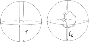
Figure 1. Knotting of a band $b_{K}$

The above construction is called in what follows an annulus rim-surgery, since it looks like the rim-surgery of Fintushel and Stern [5], except that we tie two strands simultaneously, rather then one. Recall that the usual rim-surgery is applied in [5] to surfaces $F\subset X$ which are primitively embedded, that is $\pi_{1}(X\smallsetminus F)=0$, which is not the case for the algebraic curves in $\mathbb{C}\rm{P}^{2}$ of degree $>1$. The primitivity condition is required to preserve the fundamental group of $X\smallsetminus F$ throughout the knotting. An annulus rim-surgery may preserve a non-trivial group $\pi_{1}(X\smallsetminus F)$, if we require commutativity of $\pi_{1}(X\smallsetminus(F\cup M))$, instead of primitivity of the embedding.

Proposition 1.2.

Assume that $X$ is a simply connected closed $4$-manifold, $F\subset X$ is an oriented closed surface with an annulus-membrane $M$ of index $0$, $\phi:U\to S^{1}\times D^{3}$ is a trivialization like described above and $K\subset S^{3}$ is any knot. Assume furthermore that $F\smallsetminus\partial M$ is connected and the group $\pi_{1}(X\smallsetminus(F\cup M))$ is abelian. Then the group $\pi_{1}(X\smallsetminus F_{K,\phi})$ is cyclic and isomorphic to $\pi_{1}(X\smallsetminus F)$.

1.3. Maximal nest curves

To prove Theorem 1.1, I apply an annulus rim-surgery inside $X=\mathbb{C}\rm{P}^{2}$ letting $F={\mathbb{C}}A$ be the complex point set of a suitable non-singular real algebraic curve, containing an annulus, $M$, among the connected components of $\mathbb{R}\rm{P}^{2}\smallsetminus{\mathbb{R}}A$, where ${\mathbb{R}}A={\mathbb{C}}A\cap\mathbb{R}\rm{P}^{2}$ is the real locus of the curve.

One may take, for instance, a real algebraic curve ${\mathbb{C}}A$ of degree $d$, with a maximal nest real scheme. Such a curve for $d=2k$ is constructed by a small real perturbation of a union of $k$ real conics, whose real parts (ellipses) are ordered by inclusion in $\mathbb{R}\rm{P}^{2}$. For $d=2k+1$, we add to such conics a real line not intersecting the conics in $\mathbb{R}\rm{P}^{2}$ and then perturb the unions. The real part, ${\mathbb{R}}A$, of our non-singular curve contains $k$ components, $O_{1},\dots,O_{k}$, called ovals (just deformed ellipses). We order the ovals so that $O_{i}$ lies inside $O_{i+1}$ and denote by $R_{i}$ the annulus-component of $\mathbb{R}\rm{P}^{2}\smallsetminus{\mathbb{R}}A$ between $O_{i}$ and $O_{i+1}$ for $i=1,\dots,k-1$. $R_{0}$ is a topological disk bounded from outside by $O_{1}$, and $R_{k}$ is the component bounded from inside by $O_{k}$.

The closures, $\rm{Cl}(R_{i})$, for $i=1,\dots,k-1$ are obviously $0$-framed annulus-membranes on ${\mathbb{C}}A$. For simplicity, let us choose $M=\rm{Cl}(R_{1})$.

Proposition 1.3.

The assumptions of Proposition 1.2 hold if we put $X=\mathbb{C}\rm{P}^{2}$, let $F={\mathbb{C}}A$ be a maximal nest real algebraic curve of degree $d\geq 5$ and choose $M=\rm{Cl}(R_{1})$.

1.4. Proof of Theorem 1.1 for even $d$

Assuming that the class $[F]\in H_{2}(X;{\mathbb{Z}}/2)$ vanishes, one can consider a double covering $p:Y\to X$ branched along $F$; such a covering is unique if we require in addition that $H_{1}(X;{\mathbb{Z}}/2)=0$. Similarly, we consider the double coverings $Y(K,\phi)\to X$ branched along $F_{K,\phi}$. To prove non-equivalence of pairs $(\mathbb{C}\rm{P}^{2},F_{K,\phi})$ for some family of knots $K$, it is enough to show that $Y(K,\phi)$ are not pairwise diffeomorphic. To show it, I use that $Y(K,\phi)$ is diffeomorphic to the $4$-manifolds $Y_{K\#K}$ obtained from $Y$ by a surgery introduced in [4] (I call it FS-surgery).

Proposition 1.4.

The above $Y(K,\phi)$ is diffeomorphic to a $4$-manifold obtained from $Y$ by the FS-surgery along the torus $T=p^{-1}(M)$ via the knot $K\#K\subset S^{3}$.

To distinguish the diffeomorphism types of $Y_{K\#K}$ one can use the formula of Fintushel and Stern [4] for SW-invariants of a $4$-manifold $Y$ after FS-surgery along a torus $T\subset Y$. Recall that this formula can be applied if the SW-invariants of $Y$ are well-defined and a torus $T$, realizing a non-trivial class $[T]\in H_{2}(Y)$, is c-embedded (the latter means that $T$ lies as a non-singular fiber in a cusp-neighborhood in $Y$, cf. [4]). Being an algebraic surface of genus $\geq 1$, the double plane $Y$ has well-defined SW-invariants. The conditions on $T$ are also satisfied.

Proposition 1.5.

Assume that $X$, $F$ and $M$ are like in Proposition 1.2, $[F]\in H_{2}(X;{\mathbb{Z}}/2)$ vanishes and $p:Y\to X$ is like above. Then the torus $T=p^{-1}(M)$ is primitively embedded in $Y$ and therefore $[T]\in H_{2}(Y)$ is an infinite order class. If, moreover, $X$, $F$ and $M$ are chosen like in Proposition 1.3, then $T\subset Y$ is c-embedded.

Recall that the product formula [4]

$$SW_{Y_{K}}=SW_{Y}{}^{.}\Delta_{K}(t),\ \text{ where }t=\exp(2[T])$$

expresses the Seiberg-Witten invariants (combined in a single polynomial) of the manifold $Y_{K}$, obtained by an FS-surgery, in terms of the Seiberg-Witten invariants of $Y$ and the Alexander polynomial, $\Delta_{K}(t)$, of $K$.

This formula implies that the basic classes of $Y_{K}$ can be expressed as $\pm\beta+2n[T]$, where $\pm\beta\in H_{2}(Y)$ are the basic classes of $Y$ and $|n|\leq\deg(\Delta_{K}(t))$, are the degrees of the non-vanishing monomials in $\Delta_{K}(t)$. So, if $[T]$ has infinite order, then the manifolds $Y(K,\phi)\cong Y_{K\#K}$ differ from each other by their SW-invariants, and moreover, by the numbers of their basic classes, for an infinite family of knots $K$, since the number of the basic classes is determined by the number of the terms in $\Delta_{K\#K}=(\Delta_{K})^{2}$ (one can take any family of knots with Alexander polynomials of distinct degrees). ∎

1.5. A generalization

More generally, one can produce “fake algebraic curves” under the following conditions.

Theorem 1.6.

Assume that $F$ is a non-singular connected curve in a simply connected complex surface $X$, which admits a deformation degenerating $F$ into an irreducible curve $F_{0}\subset X$, with a singularity of the type $X_{9}$, such that the fundamental group $\pi_{1}(X\smallsetminus F_{0})$ is abelian. Then there exists an infinite family of surfaces $F_{K,\phi}\subset X$ homeomorphic to $F$ and realizing the same homology class as $F$, having the same fundamental group of the complement, but with the smoothly non-equivalent pairs $(X,F_{K,\phi})$.

I remind that $X_{9}$-singularity is a point where $4$ non-singular branches meet pairwise transversally. Nori’s theorem [7] gives conditions under which $\pi_{1}(X\smallsetminus F_{0})$ must be abelian. For instance, it is so if $A_{0}$ has no other singularities except $X_{9}$ and $A\circ A>16$.

Remark 1.2.

The claim of Theorem 1.6 holds also if $F_{0}$ has a more complicated then $X_{9}$ singularity, provided the group $\pi_{1}(X\smallsetminus F_{0})$ is abelian.

2. Commutativity of the fundamental group throughout the knotting

Lemma 2.1.

The assumptions of Proposition 1.2 imply that $\pi_{1}(X\smallsetminus(F\cup M))=\pi_{1}(X\smallsetminus F)$ is cyclic with a generator presented by a loop around $F$.

Proof.

The Alexander duality in $X$ combined with the exact cohomology sequence of a pair $(X,F\cup M)$ gives

$$H_{1}(X\smallsetminus(F\cup M))\cong H^{3}(X,F\cup M)=H^{2}(F\cup M)/i^{*}H^{2}(X)$$

where $i:F\cup M\to X$ is the inclusion map. If $F$ is oriented and $F\smallsetminus\partial M$ is connected, then the Mayer-Vietoris Theorem yields $H^{2}(F\cup M)\cong H^{2}(F)\cong{\mathbb{Z}}$, and thus $H_{1}(X\smallsetminus(F\cup M))\cong H_{1}(X\smallsetminus F)$ is cyclic with a generator presented by a loop around $F$. The same property holds for the fundamental groups of $X\smallsetminus(F\cup M)$ and $X\smallsetminus F$, since they are abelian by the assumption of Proposition 1.2. ∎

Proof of Proposition 1.2. Put $X_{0}=\rm{Cl}(X\smallsetminus U)$. Then $\partial X_{0}=\partial U\cong S^{1}\times S^{2}$ and $\partial U\smallsetminus F$ is a deformational retract of $U\smallsetminus(F\cup M)$, so

$$\pi_{1}(X_{0}\smallsetminus F)=\pi_{1}(X\smallsetminus(F\cup M))$$

Since this group is cyclic and is generated by a loop around $F$, the inclusion homomorphism $h:\pi_{1}(\partial U\smallsetminus F)\to\pi_{1}(X_{0}\smallsetminus F)$ is epimorphic and thus $\pi_{1}(X_{0}\smallsetminus F)=\pi_{1}(\partial U\smallsetminus F)/k$, where $k$ is the kernel of $h$.

Applying the Van Kampen theorem to the triad $(X_{0}\smallsetminus F,U\smallsetminus F_{K,\phi},\partial U\smallsetminus F)$, we conclude that $\pi_{1}(X\smallsetminus F_{K,\phi})\cong\pi_{1}(U\smallsetminus F_{K,\phi})/j(k)$, where $j:\pi_{1}(\partial U\smallsetminus F)\to\pi_{1}(U\smallsetminus F_{K,\phi})$ is the inclusion homomorphism. Furthermore, in the splitting

$$\pi_{1}(U\smallsetminus F_{K,\phi})\cong\pi_{1}(S^{1}\times(D^{3}\smallsetminus f_{K}))\cong{\mathbb{Z}}\times\pi_{1}(D^{3}\smallsetminus f_{K})$$

factorization by $j(k)$ kills the first factor ${\mathbb{Z}}$ and adds some relations to $\pi_{1}(D^{3}\smallsetminus f_{K})$, one of which effects to $\pi_{1}(D^{3}\smallsetminus f_{K})$ as if we attach a $2$-cell along a loop, $m_{b}$, going once around the band $b_{K}$ (to see it, note that factorization by $k$ leaves only one generator of $\pi_{1}(\partial D^{3}\smallsetminus f_{K})=\pi_{1}(S^{2}\smallsetminus\{4\text{\rm{pts}}\})$). Attaching such a $2$-cell effects to $\pi_{1}$ as connecting together a pair of the endpoints of $f_{K}$, which transforms $f_{K}$ into an arc (see Figure 2). This arc is unknotted and thus factorization by $j(k)$ makes $\pi_{1}(D^{3}\smallsetminus f_{K})$ cyclic and leaves $\pi_{1}(X\smallsetminus F_{K,\phi})$ isomorphic to $\pi_{1}(X_{0}\smallsetminus F)\cong\pi_{1}(X\smallsetminus(F\cup M))\cong\pi_{1}(X\smallsetminus F)$. ∎

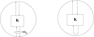
Figure 2. Gluing a $2$-cell along $m_{b}$ effects as transforming $f_{K}$ into an unknotted arc

Proof of Proposition 1.3. All the assumptions of Proposition 1.2 except the last two are obviously satisfied. It is well known that ${\mathbb{C}}A\smallsetminus{\mathbb{R}}A$ splits for a maximal nest curve ${\mathbb{C}}A$ into a pair of connected components permuted by the complex conjugation, and thus, ${\mathbb{C}}A\smallsetminus\partial M$ is connected, provided $\partial M\varsubsetneq{\mathbb{R}}A$, which is the case for $d\geq 5$. So, it is only left to check that the group $\pi_{1}(\mathbb{C}\rm{P}^{2}\smallsetminus({\mathbb{C}}A\cup M))$ is abelian.

There are several ways to check it. For instance, one can refer to my old work [1] containing computation of the homotopy type of $\mathbb{C}\rm{P}^{2}\smallsetminus({\mathbb{C}}A\cup\mathbb{R}\rm{P}^{2})$ and, in particular, of its fundamental group (see also §4 in [3]). This computation concerns a real curve ${\mathbb{C}}A\subset\mathbb{C}\rm{P}^{2}$ if it is an $L$-curve, i.e., ${\mathbb{C}}A$ can be obtained by a non-singular perturbation from a curve ${\mathbb{C}}A_{0}={\mathbb{C}}L_{1}\cup\dots\mathbb{C}L_{d}$ splitting into $d$ real lines, ${\mathbb{C}}L_{i}$, in a generic position. The maximal nest curves, ${\mathbb{C}}A\subset\mathbb{C}\rm{P}^{2}$, can be easily constructed as $L$-curves, and the result of [1] gives a presentation $\pi=\pi_{1}(\mathbb{C}\rm{P}^{2}\smallsetminus({\mathbb{C}}A\cup\mathbb{R}\rm{P}^{2}))=\langle a,b\,|\,a^{d}b^{d}=1\rangle$, where $a$, $b$ are represented by loops around the two connected components of ${\mathbb{C}}A\smallsetminus{\mathbb{R}}A$. More specifically, a basis point and these loops can be taken on the conic $C=\{x^{2}+y^{2}+z^{2}=0\}\subset\mathbb{C}\rm{P}^{2}$, which have the real point set empty. The group $\pi_{1}(\mathbb{C}\rm{P}^{2}\smallsetminus({\mathbb{C}}A\cup M))$ is obtained from $\pi$ by adding the relations corresponding to puncturing the components $R_{i}$, $0\leq i\leq k$, $i\neq 1$, of $\mathbb{R}\rm{P}^{2}\smallsetminus{\mathbb{R}}A$ (here $d=2k$ or $d=2k+1$). Such a relation (as we puncture $R_{i}$) is $a^{d-i}b^{i}=b^{d-i}a^{i}=1$, see [1], or §4 in [3]. A pair of the relations for $i=2$ and $i=3$ implies that $a=b$.

The arguments from [1] and [3] relevant to the above calculation are briefly summarized in the Appendix. ∎

Remark 2.1.

It follows from the proof above that $\pi_{1}(\mathbb{C}\rm{P}^{2}\smallsetminus({\mathbb{C}}A\cup M))$ is not abelian and ${\mathbb{C}}A\smallsetminus\partial M$ is not connected for a maximal nest quartic, ${\mathbb{C}}A$.

3. The double surgery in the double covering

Proof of Proposition 1.4. The proof is based on the following two observations. First, we notice that $Y(K,\phi)$ is obtained from $Y$ by a pair of FS-surgeries along the tori parallel to $T$, then we notice that such pair of surgeries is equivalent to a single FS-surgery along $T$. The both observations are corollaries of Lemma 2.1 in [5], so, I have to recall first the construction from [4], [5].

An FS-surgery [4] on a $4$-manifold $X$ along a torus $T\subset X$, with the self-intersection $T\circ T=0$, via a knot $K\subset S^{3}$ is defined as a fiber sum $X\#_{T=S^{1}\times m_{K}}S^{1}\times M_{K}$, that is an amalgamated connected sum of $X$ and $S^{1}\times M_{K}$ along the tori $T$ and $S^{1}\times m_{K}\subset S^{1}\times M_{K}$. Here $M_{K}$ is a $3$-manifold obtained by the $0$-surgery along $K$ in $S^{3}$, and $m_{K}$ denotes a meridian of $K$ (which may be seen both in $S^{3}$ and in $M_{K}$). Such a fiber sum operation can be viewed as a direct product of $S^{1}$ and the corresponding $3$-dimensional operation, which I call $S^{1}$-fiber sum.

More precisely, $S^{1}$-fiber sum $X\#_{K=L}Y$ of oriented $3$-manifolds $X$ and $Y$ along oriented framed knots $K\subset X$ and $L\subset Y$ is the manifold obtained by gluing the complements $\rm{Cl}(X\smallsetminus N(K))$ and $\rm{Cl}(Y\smallsetminus N(L))$ of tubular neighborhoods, $N(K)$, $N(L)$, of $K$ and $L$ via a diffeomorphism $f:\partial N(K)\to\partial N(L)$ which identifies the longitudes of $K$ with the longitudes of $L$ preserving their orientations, and the meridians of $K$ with the meridians of $L$ reversing the orientations. As it is shown in Lemma 2.1 of [5], tying a knot $K$ in an arc in $D^{3}$ can be interpreted as a fiber sum $D^{3}\#_{m=m_{K}}M_{K}$, where $m$ is a meridian around this arc. The meridians $m$ and $m_{K}$ are endowed here with the $0$-framings ($0$-framing of a meridian makes sense as a meridian lies in a small $3$-disc). To understand this observation, it is useful to view an $S^{1}$-fiber sum with $M_{K}$ as surgering a tubular neighborhood, $N(m)$, of $m$ and replacing it by the complement, $S^{3}\smallsetminus N(K)$ of a tubular neighborhood, $N(K)$, of $K$, so that the longitudes of $m$ are glued to the meridians of $K$ and the meridians of $m$ to the longitudes of $K$. The framing of an arc in $D^{3}$ is preserved under such a fiber sum, so tying a knot in the band $b\subset D^{3}$ is equivalent to taking an $S^{1}$-fiber sum with $M_{K}$ along a meridian $m_{b}$ around $b$.

The double covering over $D^{3}$ branched along $f$ is a solid torus, $N\cong S^{1}\times D^{2}$, and the pull back of $m_{b}$ splits into a pair of circles, $m_{1},m_{2}\subset N$, parallel to $m=S^{1}\times\{0\}$. Therefore, $Y(K,\phi)$ is obtained from $Y$ by performing FS-surgery twice, along the tori

$$T_{i}=S^{1}\times m_{i}\subset p^{-1}(U)\cong S^{1}\times N,\ \ i=1,2$$

The following Lemma implies that this gives the same result as a single FS-surgery along $T=p^{-1}(M)$ via the knot $K\#K$. ∎

Lemma 3.1.

For any pair of knots, $K_{1},K_{2}$, the manifold

$$M_{K_{1}}\#_{m_{K_{1}}=m_{1}}N\#_{m_{2}=m_{K_{2}}}M_{K_{2}}$$

obtained by taking an $S^{1}$-fiber sum twice, is diffeomorphic to $N\#_{m=m_{K}}M_{K}$, for $K=K_{1}\#K_{2}$, via a diffeomorphism identical on $\partial N$.

Proof.

A solid torus $N$ can be viewed as the complement $N=S^{3}-N^{\prime}$ of an open tubular neighborhood $N^{\prime}$ of an unknot, so that $m,m_{1},m_{2}$ represent meridians of this unknot. Taking a fiber sum of $S^{3}$ with $M_{K_{i}}$ along $m_{i}=m_{K_{i}}$ is equivalent to knotting $N^{\prime}$ in $S^{3}$ via $K_{i}$. So, performing $S^{1}$-fiber sum twice, along $m_{1}$ and $m_{2}$, we obtain the same result as after taking fiber sum along $m$ once, via $K=K_{1}\#K_{2}$. ∎

Remark 3.1.

The above additivity property can be equivalently stated as

$$M_{K_{1}}\#_{m_{K_{1}}=m_{K_{2}}}M_{K_{2}}\cong M_{K_{1}\#K_{2}}$$

Proof of Proposition 1.5. Lemma 2.1 implies that, in the assumptions of Proposition 1.2, $\pi_{1}(Y\smallsetminus(F\cup T))$ is a cyclic group with a generator represented by a loop around $F$. Thus, $\pi_{1}(Y\smallsetminus T)=0$ and, by the Alexander duality, $H_{3}(Y,T)=H^{1}(Y\smallsetminus T)=0$, which implies that $[T]\in H_{2}(Y)$ has infinite order.

To check that $T$ is c-embedded it is enough to observe that there exists a pair of vanishing cycles on $T$, or more precisely, a pair of $D^{2}$-membranes, $D_{1},D_{2}\subset Y$, on $T$, having $(-1)$-framing and intersecting at a unique point $x\in T$, so that $[\partial D_{1}],[\partial D_{2}]$ form a basis of $H_{1}(T)$. In the setting of Proposition 1.3, $Y\to\mathbb{C}\rm{P}^{2}$ is a double covering branched along a maximal nest curve ${\mathbb{C}}A$ and $T$ is a connected component of the real part of $Y$ (with respect to a certain real structure on $Y$ lifted from $\mathbb{C}\rm{P}^{2}$). Two nodal degenerations of ${\mathbb{C}}A$ shown on the top part of Figure 3 give nodal degenerations of the double covering $Y$.

In the first of the degenerations of ${\mathbb{C}}A$, a node appears as an oval $O_{1}$ is collapsed into a point. In the second degeneration a crossing-like node can be seen as the fusion point of the ovals $O_{1}$ and $O_{2}$. Existence of such degenerations for our explicitly constructed curve ${\mathbb{C}}A$ is known and trivial. Another simple observation (which is obvious for quartics and thus follows for any maximal nest curve of a higher degree) is that our pair of nodal degenerations can be united into one cuspidal degeneration. This means in particular that the two vanishing cycles in $Y$ intersect transversally at a single point.

Furthermore, our complex vanishing cycles in $Y$ can be chosen conj-invariant. Being a $(-2)$-sphere, each of such complex cycles is divided by its real pair into a pair of $(-1)$-discs. Choosing one disc from each pair, we obtain $D_{1}$ and $D_{2}$ that we need.

It is easy to view these $(-2)$-spheres and the $(-1)$-disks explicitly. First, note that $R_{0}$ is a $(-1)$-membrane on ${\mathbb{C}}A$ and $p^{-1}(R_{0})$ is the first of the conj-symmetric vanishing cycles. The $(-1)$-disk $D_{1}$ is any of its halves. Furthermore, there is another $(-1)$-disk membrane, $Q$ on ${\mathbb{C}}A$ corresponding to the second nodal degeneration. It can be chosen conj-invariant and then is split by $Q\cap\mathbb{R}\rm{P}^{2}$ into semi-discs $Q=Q_{1}\cup Q_{2}$ permuted by conj. $Q_{i}$ is bounded by the arcs $Q\cap\mathbb{R}\rm{P}^{2}$ and $Q_{i}\cap{\mathbb{C}}A$. The disk $D_{2}$ is any of the discs $p^{-1}(Q_{i})$. ∎

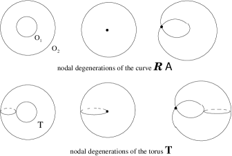
Figure 3. Nodal degenerations of ${\mathbb{R}}A$ providing $(-1)$-framed $D^{2}$-membranes on $T$ $f_{K}$ into an unknotted arc

4. The case of $d$-fold branched covering

Consider as before a maximal nest curve, ${\mathbb{C}}A\subset\mathbb{C}\rm{P}^{2}$, of degree $d\geq 2$, and ${\mathbb{C}}A_{K,\phi}$ obtained from ${\mathbb{C}}A$ via an annulus rim-surgery along $R_{1}$, but now let us denote by $p:Y\to\mathbb{C}\rm{P}^{2}$ and $Y(K,\phi)\to\mathbb{C}\rm{P}^{2}$ the $d$-fold coverings branched along ${\mathbb{C}}A$ and ${\mathbb{C}}A_{K,\phi}$ respectively. Consider a $d$-fold covering $N\to D^{3}$ branched along $f$. The pull-back of $m_{b}$ consists of $d$ circles, $m_{1},\dots,m_{d}$, which are cyclically ordered. Using a homeomorphism $(D^{3},f)\cong(D^{2}\times[0,1],\{z_{1},z_{2}\}\times[0,1])$, where $\{z_{1},z_{2}\}\subset\rm{Int}(D^{2})$, we present $N$ as $F\times[0,1]$, where $F$ is a sphere with $d$ holes. The circles $m_{i}$ go around these holes. An annulus rim-surgery in $\mathbb{C}\rm{P}^{2}$ along $m_{b}\times S^{1}\subset D^{3}\times S^{1}$, is covered by $d$ copies of FS-surgery along the tori $T_{i}=m_{i}\times S^{1}\subset N\times S^{1}$.

The following observation implies that the Fintushel-Stern formula for Seiberg-Witten invariants can be applied in this setting.

Proposition 4.1.

Each of the tori $T_{i}$ is primitively c-embedded in the complement of the others.

Proof.

A pair of $(-1)$-disc membranes, $D_{1}^{i}$, $D_{2}^{i}$, on each of $T_{i}$ is constructed like in the proof of Proposition 1.5. Namely, $p^{-1}(R_{0})$ consists of $d$ disks which yield the disks $D_{1}^{i}$, that are glued along $\{\text{pt}\}\times S^{1}\subset m_{i}\times S^{1}$.

Furthermore, $p^{-1}(Q_{1})$ splits also into $d$ disks, $Q_{1}^{1},\dots,Q_{1}^{d}$. Let us choose their orientations induced from a fixed orientation of $Q_{1}$ and cyclically order in accord with the ordering of $T_{i}$, then the unions $Q_{1}^{i}\cup(-Q_{1}^{i+1})$ provide the required discs $D_{2}^{i}$, which are glued along $m_{i}\times\{\text{pt}\}$. More precisely, $D_{1}^{i}$ are the parts of the components of $p^{-1}(R_{0})$ bounded by the intersections of the components with the tori $T_{i}$, whereas $D_{1}^{i}$ are obtained from $Q_{1}^{i}\cup(-Q_{1}^{i+1})$ by a small shift making them membranes on $T_{i}$. ∎

Next, we observe that there exists only one linear dependence relation between the classes $[T_{i}]\in H_{2}(Y)$.

Proposition 4.2.

The inclusion map $H_{2}(\bigcup_{i}T_{i})\to H_{2}(Y)$ has kernel ${\mathbb{Z}}$ generated by the relation $\Sigma_{i=1}^{d}[T_{i}]=0$. Here $T_{i}$ are oriented uniformly in accord with some fixed orientation of $m_{b}\times S^{1}$.

Proof.

It is enough to show that $\pi_{1}(Y\smallsetminus(N\times S^{1}))=0$, since it implies that $H_{3}(Y,N\times S^{1})\cong H^{1}(Y\smallsetminus(N\times S^{1}))=0$ and thus the inclusion map $H_{2}(N\times S^{1})\to H_{2}(Y)$ is monomorphic. The first inclusion map in the composition $H_{2}(\bigcup_{i}T_{i})\to H_{2}(N\times S^{1})\to H_{2}(Y)$ that we analyze, is just $H_{1}(\partial F)\otimes H_{1}(S^{1})\to H_{1}(F)\otimes H_{1}(S^{1})$, and has kernel $H_{2}(F,\partial F)\otimes H_{1}(S^{1})\cong{\mathbb{Z}}$, as stated in the Proposition.

Now note that $p^{-1}(R_{1})$ is a deformational retract (spine) of $N\times S^{1}$, so it is enough to check the triviality of $\pi_{1}(Y\smallsetminus(p^{-1}(R_{1}))$. This triviality follows from that $\pi_{1}(\mathbb{C}\rm{P}^{2}\smallsetminus({\mathbb{C}}A\cup R_{1}))$ is ${\mathbb{Z}}/d$, with a generator represented by a loop around ${\mathbb{C}}A$ (say, by the computation in [1] reproduced in the Appendix), and thus $\pi_{1}(Y\smallsetminus p^{-1}({\mathbb{C}}A\cup R_{1}))=0$. ∎

Proposition 4.2 together with the Fintushel-Stern formula [4] guarantees that the Seiberg-Witten invariants of $Y(K,\phi)$ are distinct for some sequence of knots $K$ with increasing degrees of $\Delta_{K}(t)$.

Proof of Theorem 1.6 The case of a primitive class $[F]\in H_{2}(X)$ is considered in [5]. More precisely, the assumptions in Theorem 1.1 in [5] are satisfied because our condition on the fundamental group yields that $\pi_{1}(X\smallsetminus F)$ is abelian and thus trivial, existence of an irreducible deformation of $F$ implies that $F\circ F\geq 0$, and $X_{9}$-degeneration guarantees that $F$ is not a rational curve.

If $[F]$ is divisible by $d\geq 2$, then we consider a $d$-fold covering, $p:Y\to X$, branched along $F$ and perform an annulus rim-surgery on $F$ along a membrane $M$ defined as follows. Consider a local topological model of the singularity $X_{9}$, defined in ${\mathbb{C}}^{2}$ by the equation $(x^{2}+y^{2})(x^{2}+2y^{2})=0$, and a model of its perturbation, $(x^{2}+y^{2}-4\varepsilon)(x^{2}+2y^{2}-\varepsilon)=\delta$, where $\varepsilon,\delta\in{\mathbb{R}}$, $0<\!\!<\delta<\!\!<\varepsilon<\!\!<1$. The real locus of a perturbed singularity contains a pair of ovals which bound together in ${\mathbb{R}}^{2}$ an annulus that we take as $M$.

The assumptions of Theorem 1.6 imply those of Proposition 1.2. Namely, irreducibility of $F_{0}$ implies that $F\smallsetminus{\partial M}$ is connected and commutativity of $\pi_{1}(X\smallsetminus F_{0})$ implies commutativity of $\pi_{1}(X\smallsetminus(F\cup M))$ via Van Kampen theorem. Moreover, the singularity $X_{9}$ provides the topological picture that was used in the above proof of Theorem 1.1, in the case of $d$-fold covering. Namely, $X_{9}$ yields the both $(-1)$-disk membranes that were used to show that the Fintushel and Stern formula can be applied to $Y$. ∎

Remark 4.1.

Note that to apply the formula [5] it is not required that $b_{2}^{+}(Y)>1$. Nevertheless, it is so, because $b_{2}^{+}(Y)\geq d$, which can be proved by observing $d$ linearly independent pairwise orthogonal classes in $H_{2}(Y)$, having non-negative squares. One of these classes is $[F]$, and the other $(d-1)$ come from $p^{-1}(M)$, due to Proposition 4.2 (each of these $(d-1)$ classes has self-intersection $0$).

5. Appendix: The topology of $\mathbb{C}\rm{P}^{2}\smallsetminus(\mathbb{R}\rm{P}^{2}\cup{\mathbb{C}}A)$ for $L$-curves ${\mathbb{C}}A$

Let ${\mathbb{C}}A_{0}={\mathbb{C}}L_{1}\cup\dots\cup{\mathbb{C}}L_{d}\subset\mathbb{C}\rm{P}^{2}$ denote the complex point set of a real curve of degree $d$ splitting into $d$ lines, ${\mathbb{C}}L_{i}$. Put $\widetilde{V}=C\cap{\mathbb{C}}A_{0}$, where $C$ is the conic from the proof of Proposition 1.3. Our first observation is that $C\smallsetminus\widetilde{V}$ is a deformational retract of $\mathbb{C}\rm{P}^{2}\smallsetminus(\mathbb{R}\rm{P}^{2}\cup{\mathbb{C}}A_{0})$, and moreover, the latter complement is homeomorphic to $(C\smallsetminus\widetilde{V})\times\rm{Int}(D^{2})$. To see it, it suffices to note that $\mathbb{C}\rm{P}^{2}\smallsetminus\mathbb{R}\rm{P}^{2}$ is fibered over $C$ with a $2$-disc fiber, each fiber being a real semi-line, that is a connected component of ${\mathbb{C}}L\smallsetminus{\mathbb{R}}L$ for some real line ${\mathbb{C}}L\subset\mathbb{C}\rm{P}^{2}$, where ${\mathbb{R}}L={\mathbb{C}}L\cap\mathbb{R}\rm{P}^{2}$. This fibering maps a semi-line into its intersection point with $C$.

It is convenient to view the quotient $C/\text{\rm{conj}}$ of the conic $C$ by the complex conjugation as the projective plane, $\widehat{\mathbb{R}\rm{P}}^{2}$, dual to $\mathbb{R}\rm{P}^{2}\subset\mathbb{C}\rm{P}^{2}$, since each real line, ${\mathbb{C}}L$, intersects $C$ in a pair of conjugated points. If we let $V=\{l_{1},\dots,l_{d}\}\subset\widehat{\mathbb{R}\rm{P}}^{2}$ denote the set of points $l_{i}$ dual to the lines ${\mathbb{R}}L_{i}\subset\mathbb{R}\rm{P}^{2}$, then $\widetilde{V}=q^{-1}(V)$, where $q:C\to C/\text{\rm{conj}}$ is the quotient map.

The information about a perturbation of ${\mathbb{C}}A_{0}$ is encoded in a genetic graph of a perturbation, $\Gamma\subset\widehat{\mathbb{R}\rm{P}}^{2}$. The graph $\Gamma$ is a complete graph with the vertex set $V$, whose edges are line segments. Note that there exist two topologically distinct perturbations of a real node of ${\mathbb{R}}A_{0}$ at $p_{ij}={\mathbb{R}}L_{i}\cap{\mathbb{R}}L_{j}$, as well as there exist two line segments in $\widehat{\mathbb{R}\rm{P}}^{2}$ connecting the vertices $l_{i},l_{j}\in V$. Let ${\mathbb{R}}A$ denotes a real curve obtained from ${\mathbb{R}}A_{0}$ by a sufficiently small perturbation. Then the edge of $\Gamma$ connecting $l_{i}$ and $l_{j}$ contains the points dual to those lines passing through $p_{i,j}$ which do not intersect ${\mathbb{R}}A$ locally, in a small neighborhood of $p_{i,j}$.

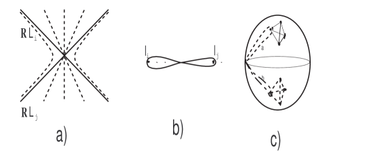
Figure 4. a) A perturbation of a real node; the dashed lines are dual to the points of an edge of $\Gamma$; b) A figure-eight loop along an edge of $\Gamma$; c) The loops in $C\smallsetminus\widetilde{V}$ representing generators “a” and “b”

The complement $\mathbb{C}\rm{P}^{2}\smallsetminus({\mathbb{C}}A\cup\mathbb{R}\rm{P}^{2})$ turns out to be homotopy equivalent to a $2$-complex obtained from $C\smallsetminus\widetilde{V}$ by adding $2$-cells glued along a figure-eight shaped loops along the edges of $\widetilde{\Gamma}=q^{-1}(\Gamma)\subset C$. Such $2$-cells identify pairwise certain generators of $\pi_{1}(C\smallsetminus\widetilde{V})$ “along the edges” of $\widetilde{\Gamma}$ (cf. [3] for details). This easily implies that the group $\pi_{1}(\mathbb{C}\rm{P}^{2}\smallsetminus({\mathbb{C}}A\cup\mathbb{R}\rm{P}^{2}))$ is generated by a pair of elements, $a$ and $b$, represented by a pair of loops in $C\smallsetminus\widetilde{V}$ around a pair of conjugated vertices of $\widetilde{V}$.

For example, for a maximal nest curve, the graph $\Gamma$ is contained in an affine part of $\widehat{\mathbb{R}\rm{P}}^{2}$, i.e., has no common points with some line in $\widehat{\mathbb{R}\rm{P}}^{2}$, namely, with a line dual to a point inside the inner oval of the nest. Therefore, the graph $\widetilde{\Gamma}$ splits into two connected components separated by a big circle in $C$. A loop around any vertex of $\widetilde{V}$ from one of these components represents $a$, and a loop around a vertex from the other component represents $b$. It is trivial to observe also the relation $a^{d}b^{d}=1$ (which is indeed a unique relation in the case of maximal nest curves).

As we puncture $\mathbb{R}\rm{P}^{2}$ at a point $x\in\mathbb{R}\rm{P}^{2}\smallsetminus{\mathbb{R}}A_{0}$, we attach a $2$-cell to $C\smallsetminus\widetilde{V}$ along the big circle $S_{x}\subset C$ dual to $x$. If $x$ moves across a line ${\mathbb{R}}L_{i}$, then $S_{x}$ moves across the pair of points $q^{-1}(l_{i})$. Since a small perturbation and puncturing are located at distinct points of $\mathbb{C}\rm{P}^{2}$ and can be done independently, it is not difficult to see that if we choose $x\in R_{i}$ (in the case of a maximal nest curve ${\mathbb{C}}A$), then the big circle $S_{x}$ cuts $C$ into the hemispheres, one of which contains $i$ vertices from one component of $\widetilde{\Gamma}$ and $d-i$ vertices from the other component. This gives relations $a^{i}b^{d-i}=a^{d-i}b^{i}=1$.

References

- [1] S. Finashin Topology of the Complement of a Real Algebraic Curve in , Zap. Nauch. Sem. LOMI 122 (1982), 137–145
- [2] S. Finashin, Knotting of algebraic curves in , math.GT/9907108, to appear in “Topology”
- [3] S. Finashin, M. Kreck, O. Viro, Non-diffeomorphic but homeomorphic knottings of surfaces in the -sphere Spr. Lecture Notes in Math. 1346 (1988), 157–198
- [4] R. Fintushel, R. Stern, Knots, Links and -manifolds Invent. Math. 134 (1988), 2, 363–400
- [5] R. Fintushel, R. Stern, Surfaces in -manifolds Math. Res. Lett., 4 (1997), 907–914
- [6] R. Kirby, Problems in Low-dimensional Topology, 1996
- [7] M. V. Nori, Zariski conjecture and related problems Ann. Sci. Ec. Norm. Sup., 4 Ser., 16 (1983), 305–344