Filling Length in Finitely Presentable Groups

Abstract

Filling length measures the length of the contracting closed loops in a null-homotopy. The filling length function of Gromov for a finitely presented group measures the filling length as a function of length of edge-loops in the Cayley 2-complex. We give a bound on the filling length function in terms of the log of an isoperimetric function multiplied by a (simultaneously realisable) isodiametric function.

1 Isoperimetric and isodiametric functions

Given a finitely presented group $\Gamma=\left<\mathcal{A}\left|\mathcal{R}\right.\right>$ various filling invariants arise from considering reduced words $w$ in the free group $F(\mathcal{A})$ such that $w=_{\Gamma}1$. Such null-homotopic words are characterised by the existence of an equality in $F(\mathcal{A})$

$$w=\prod_{i=1}^{N}{u_{i}^{-1}r_{i}u_{i}}$$ (1)

for some $N\in\mathbb{N}$, relators $r_{i}\in R$, and words $u_{i}\in F(\mathcal{A})$. A van Kampen diagram provides a geometric means of displaying such an equality - see [2, page 155], [10, pages 235ff]. This gives a notion of a homotopy disc for $w$. Then, in analogy with null-homotopic loops in a Riemannian manifold, we can associate various filling invariants to the possible van Kampen diagrams for null-homotopic words $w$.

Many such filling invariants are discussed by Gromov in Chapter 5 of [9]. We will be concerned with three: the Dehn function (also known as the optimal isoperimetric function), the optimal isodiametric function and the filling length function.

The first two of these invariants are better known than the third - see for example [6] and [7]. Let $|w|$ denote the length of a reduced word in $F(\mathcal{A})$. If $w=_{\Gamma}1$ then define $\text{Area}(w)$ to be the minimum number $N$ such that there is a van Kampen diagram for $w$ with $N$ faces (i.e. 2-cells). The diameter of a van Kampen diagram $\mathcal{D}$ is the supremum over all vertices $v$ of $\mathcal{D}$ of the shortest path in the 1-skeleton of $\mathcal{D}$ that connects $v$ to the base point of $\mathcal{D}$. Define $\text{Diam}(w)$ to be the least diameter of van Kampen diagrams for $w$. Then the Dehn function $f_{0}:\mathbb{N}\to\mathbb{N}$ and optimal isodiametric function $g_{0}:\mathbb{N}\to\mathbb{N}$ for $\Gamma=\left<\mathcal{A}\left|\mathcal{R}\right.\right>$ are defined by

$$f_{0}(n) := \max\left\{\text{Area}(w):w\in F(\mathcal{A}),|w|\leq n\text{ and }w=_{\Gamma}1\right\},$$

$$g_{0}(n) := \max\left\{\text{Diam}(w):w\in F(\mathcal{A}),|w|\leq n\text{ and }w=_{\Gamma}1\right\}.$$

We say that $f$ and $g$ are respectively isoperimetric and isodiametric functions for $\Gamma$ if $f_{0}(n)\leq f(n)$ and $g_{0}(n)\leq g(n)$ for all $n$.

As defined the Dehn and the optimal isodiametric function are dependent on the choice of presentation of $\Gamma$. However different presentations produce $\simeq$-equivalent functions. From an algebraic point of view the Dehn function $f_{0}(n)$ is the least $N$ such that for any null-homotopic word $w$ with $|w|\leq n$ there is an equality in $F(\mathcal{A})$ of the form of equation (1). Similarly (but this time only up to $\simeq$-equivalence) the optimal isodiametric function is the optimal bound on the length of the conjugating words $u_{i}\in F(\mathcal{A})$.

2 The filling length function

In the context of a Riemannian manifold $X$ consider contracting a null-homotopic loop $\gamma:[0,1]\to X$ based at $x_{0}\in X$ to the constant loop at $x_{0}$. By definition there is some continuous $H:[0,1]\times[0,1]\to X$ denoted by $H_{t}(s)=H(t,s)$ with $H_{0}=\gamma$, $H_{1}(s)=x_{0}$ for all $s$, and $H_{t}(0)=H_{t}(1)=x_{0}$ for all $t$. Filling length is a control on the length of the loops $H_{t}$. So the filling length of $H$ is the supremum of the lengths of the loops $H_{t}$ for $t\in[0,1]$. And the filling length of $\gamma$ is the infimum of the filling lengths of all possible null-homotopies $H$. So (using Gromov’s notation) define $\text{Fill}_{0}\text{ Leng}\,\ell$ to be the supremum of the filling lengths of all null-homotopic loops $\gamma:[0,1]\to X$ of length at most $\ell$ and based at $x_{0}\in X$.

Now translate to the situation in a finitely presented group $\Gamma=\left<\mathcal{A}\left|\mathcal{R}\right.\right>$. The concept of homotopy discs is provided by van Kampen diagrams. In the combinatorial context of a van Kampen diagram $\mathcal{D}$ we use elementary homotopies. The boundary word $w$ is reduced to the constant word $1$ at the base point $x_{0}$ by successively applying two types of moves:

1. (1-cell collapse) remove pairs $(e^{1},e^{0})$ for which $e^{0}\in\partial e^{1}$ is a 0-cell which is not the base point $x_{0}$, and $e^{1}$ is a 1-cell only attached to the rest of the diagram at one 0-cell which is not $e^{0}$;

2. (2-cell collapse) remove pairs $(e^{2},e^{1})$ where $e^{2}$ is a 2-cell of $\mathcal{D}$ with $e^{1}$ an edge of $\partial e^{2}\cap\partial\mathcal{D}$ (note this does not change the 0-skeleton of $\mathcal{D}$).

Algebraically 1-cell collapse corresponds to free reduction in $F(A)$ (but not cyclic reduction since the base point $x_{0}$ is preserved). And 2-cell collapse is the substitution of $a_{2}a_{3}\ldots a_{n}$ for $a_{1}^{-1}$, where $a_{1},a_{2},\ldots,a_{n}\in\mathcal{A}^{\pm 1}$ and $a_{1}a_{2}\ldots a_{n}$ is a cyclic permutation of an element of $\mathcal{R}^{\pm 1}$. Let the filling length of $\mathcal{D}$, denoted $FL(\mathcal{D})$, be the best possible bound on the length of the boundary word as we successively apply these two types of move to reduce $w$ to $1$. Define the filling length $FL(w)$ of a null-homotopic word $w$ by

$$FL(w):=\min\left\{FL(\mathcal{D}):\mathcal{D}\text{ is a van Kampen diagram for }w\right\}.$$

Then define the filling length function $h_{0}:\mathbb{N}\to\mathbb{N}$ by

$$h_{0}(n):=\max\left\{FL(w):w\in F(\mathcal{A}),|w|\leq n\text{ and }w=_{\Gamma}1\right\}.$$

As for $f_{0}$ and $g_{0}$, observe that $h_{0}$ is independent of the presentation up to $\simeq$-equivalence.

Some relationships known between $f_{0},g_{0}$ and $h_{0}$ are as follows.

Examples

1. For a finitely presented group $\Gamma=\left<\mathcal{A}\left|\mathcal{R}\right.\right>$ with $K:=\max\left\{|r|:r\in\mathcal{R}\right\}$, we see that for all $n$

   $$g_{0}(n)\leq h_{0}(n)\leq 2Kf_{0}(n)+n.$$

   The first inequality arises since the concentric loops of length at most $h_{0}(n)$ can be followed to reach the base point. The second inequality holds because given a null-homotopic word $w$ of length at most $n$, we find $2Kf_{0}(n)+n$ is at least twice the total length of the 1-skeleton of a van Kampen diagram for $w$.

2. Filling length has also been used by Gersten and Gromov (see pages 100ff of [9]) to give an isoperimetric function:

   $$f_{0}\preceq\exp h_{0}.$$

   A null-homotopic word $w$ of length $n$ can be reduced to the identity by elementary homotopies through distinct words of length at most $h_{0}(n)$. There are at most $\exp(C\,h_{0}(n))$ such words for some constant $C>0$. This bounds the number of 2-cell collapse moves and so this number is at least $f_{0}(n)$.

3. Cohen and Gersten have given a double exponential bound for $f_{0}$ in terms of $g_{0}$ (see [3] and [6]):

   $$f_{0}(n)\preceq\exp\exp(g_{0}(n)+n).$$

4. Asynchronously combable groups have linear bounds on their filling length functions. This is a result of Gersten [8, Theorem 3.1 on page 130] where the notation $LCNH_{1}$ is in this case what we call linearly bounded filling length. In essence the homotopy can be performed by contracting in the direction of the combing, so the contracting loop always remains normal to the combing lines. (See also [7] for definitions.)

3 Logarithmic shelling of finite rooted trees

We now digress to a lemma about rooted trees. Let $\mathcal{T}$ be a finite rooted tree in which each node has valence three except for the root (valence two) and the leaves (valence one).

Let $\mathcal{F}$ be a finite forest of such trees. The visible nodes of $\mathcal{F}$ are the roots. An elementary shelling is the removal of the root of one of its trees (together with the two edges that meet that root when the tree has more than one node). A (complete) shelling is a sequence of elementary shellings ending with the empty forest. The visibility number of a shelling of $\mathcal{F}$ is the maximum number of visible vertices occurring in the shelling. The visibility number $VN(\mathcal{F})$ is the minimum visibility number of all shellings.

Let $N(\mathcal{T})$ denote the number of nodes of $\mathcal{T}$.

Lemma 1

Let the integer $d$ be determined by $2^{d}-1<N(\mathcal{T})\leq 2^{d+1}-1$. Then $VN(\mathcal{T})\leq d+1$.

Proof. To obtain this bound on $VN(\mathcal{T})$ we shall perform each elementary shelling by always choosing a tree with the least number of nodes to shell first.

We argue by induction on $N(\mathcal{T})$, where the induction begins when $N(\mathcal{T})=1$; in this case $d=0$ and $VN(\mathcal{T})=1$, as required.

For the induction step, assume that $N(\mathcal{T})>1$ with $2^{d}-1<N(\mathcal{T})\leq 2^{d+1}-1$. Removing the root of $\mathcal{T}$ produces two trees $\mathcal{T}_{1},\mathcal{T}_{2}$. We let $N(\mathcal{T}_{1})\leq N(\mathcal{T}_{2})$. Let $2^{d_{i}}-1<N(\mathcal{T}_{i})\leq 2^{d_{i}+1}-1$ for $i=1,2$. By the induction hypothesis we have $VN(\mathcal{T}_{i})\leq d_{i}+1$ for $i=1,2$. Since we shell $T_{1}$ first, we get $VN(\mathcal{T})\leq\max(VN(\mathcal{T}_{1})+1,VN(\mathcal{T}_{2}))\leq\max(d_{1}+2,d_{2}+1)$ by the induction hypothesis. There are now two cases, depending on whether $d_{1}<d_{2}$ or $d_{1}=d_{2}$.

Case 1. $d_{1}<d_{2}$. In this case $\max(d_{1}+2,d_{2}+1)=d_{2}+1\leq d+1$, so we get $VN(\mathcal{T})\leq d+1$ as required.

Case 2. $d_{1}=d_{2}$. Here $\max(d_{1}+2,d_{2}+1)=d_{1}+2$. We have $2(2^{d_{1}}-1)+1<N(\mathcal{T}_{1})+N(\mathcal{T}_{2})+1\leq 2(2^{d_{1}+1}-1)+1$, whence $2^{d_{1}+1}-1<N(\mathcal{T})\leq 2^{d_{1}+2}-1$. It follows that $d=d_{1}+1$, and $VN(\mathcal{T})\leq d+1$ as required.

This completes the induction, and the proof of Lemma 1 is complete.

Corollary 1

$VN(\mathcal{T})<\log_{2}(N(\mathcal{T})+1)+1$.

Proof. Write $2^{d}-1<N(\mathcal{T})\leq 2^{d+1}-1$, so $VN(\mathcal{T})\leq d+1<\log_{2}(N(\mathcal{T})+1)+1$, as required.

Remark. Note that since $VN(\mathcal{T})$ is an integer, the upper bound for $VN(\mathcal{T})$ in the corollary can be replaced by the least integer bounding $\log_{2}(N(\mathcal{T})+1)$ from above. Stated in this form, the result is sharp, as we see by taking $T$ to be the complete rooted tree $T(d)$ of depth $d$. In this case $T(d)$ has $2^{d+1}-1$ nodes, and the visibility number is $d+1$.

4 A bound on the filling length function

We now proceed towards our main theorem.

Definition Let $\mathcal{P}$ be a finite presentation for the group $\Gamma$. An AD-pair for $\mathcal{P}$ is a pair of functions $(f,g)$ from $\mathbb{N}$ to $\mathbb{N}$ such that for every circuit $w$ of length at most $n$ in the Cayley graph there exists a van Kampen diagram $\mathcal{D}_{w}$ with area at most $f(n)$ and diameter at most $g(n)$. Note that $f$ is an isoperimetric function and $g$ is an isodiametric function.

Examples Up to common multiplicative constants the following are examples of AD-pairs for groups $\Gamma$.

1. $(E^{x},x)$ for some $E>1$ and $(xL(x),x)$ are both AD-pairs when $\Gamma$ is an asynchronously combable group. Here the length function $L(n)$ is the maximum length of combing paths for group elements at distance at most $n$ from the identity. That $(E^{x},x)$ is an AD-pair follows from the linear bound on the filling length function and that $f_{0}\preceq\exp h_{0}$; see section 2 Example 4. In particular $(x^{2},x)$ is an AD-pair when $\Gamma$ is synchronously automatic since $\Gamma$ then admits a combing in which the combing lines are quasi-geodesics (see [4, pages 84-86]).

2. $(f(x),f(x)+x)$ where $\Gamma$ is an arbitrary finitely presented group with an isoperimetric function $f$. (See Gersten [7], Lemma 2.2.)

3. $(E^{E^{g(x)+x}},g(x))$ for some $E>1$, when $\Gamma$ is an arbitrary finitely presented group with an isodiametric function $g$. (See Gersten [6].)

4. $(x^{r},x^{r-1})$ where $\Gamma$ satisfies a polynomial isoperimetric function of degree $r\geq 2$. We postpone proof of this example to section 5.

5. $(x^{2m+1},x^{m})$ where $\Gamma_{m}$ is

   $$\left<a_{1},\ldots,a_{m},s,t,\tau\left|\,\text{for }i<m,\,s^{-1}a_{i}s=a_{i+1},\right.\right.$$

   $$\hskip 72.26999pt\left.[t,a_{i}]=[\tau,a_{i}]=[s,a_{m}]=[t,a_{m}]=[\tau,a_{m}t]=1\right>.$$

   This family of examples is due to Bridson - see [1]. He shows that in fact $x^{2m+1}$ is the optimal isoperimetric function and $x^{m}$ is the optimal isodiametric function.

Theorem 1

Let $(f,g)$ be an AD-pair for the finite presentation $\mathcal{P}$. Then $h_{0}(n)\preceq g(n)\log(f(n)+1)$ for all $n$.

We actually prove the stronger statement:

Proposition 2

Suppose $\Gamma$ is a finitely and triangularly presented group, and $w\in\Gamma$ is null-homotopic with $n:=|w|$. Given a van Kampen diagram $\mathcal{D}$ for $w$ with $D:=\text{Diam}(\mathcal{D})$ and $A:=\text{Area}(\mathcal{D})$ we find

$$FL(\mathcal{D})\leq(2D+1)(\log_{2}(A+1)+1)+4D+1+n.$$

Any finite presentation $\left<\mathcal{A}\left|\mathcal{R}\right.\right>$ for a group $\Gamma$ yields a finite triangular presentation for $\Gamma$. Such presentations are characterised by the length of relators being at most three. If $r\in\mathcal{R}$ is expressible in $F(\mathcal{A})$ as $w_{1}w_{2}$ where $|w_{1}|,|w_{2}|\geq 2$ then add a new generator $a$ to $\mathcal{A}$, and in $\mathcal{R}$ replace $r$ by $a^{-1}w_{1}$ and $aw_{2}$. A triangular presentation is achieved after a finite number of such transformations.

As $f_{0},g_{0}$ and $h_{0}$ are invariant up to $\simeq$-equivalence on change of finite presentation, Proposition 2 is sufficient to prove Theorem 1.

Proof of Proposition 2. We start by taking a maximal geodesic tree $\mathcal{T}$ in the 1-skeleton of the van Kampen diagram $\mathcal{D}$, and rooted at the base point $x_{0}$ of $\mathcal{D}$. So from any vertex of $\mathcal{D}$ there is a path in $\mathcal{T}$ to $x_{0}$ with length at most $D$.

By cutting along paths in $\mathcal{T}$ we can decompose $\mathcal{D}$ into sub-diagrams $\mathcal{D}_{i}$ where only one edge from $\partial\mathcal{D}-\mathcal{T}$ occurs in each $\mathcal{D}_{i}$. We will perform the elementary homotopy which realises the filling length bound by pushing across each of these $\mathcal{D}_{i}$ in turn, as shown in Figure 1. Then

$$\text{FL}(\mathcal{D})\leq\displaystyle{\max_{i}}\left\{\text{FL}(\mathcal{D}_{i})\right\}+n.$$ (2)

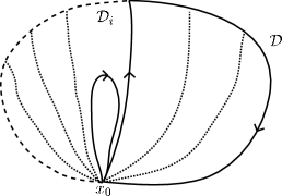
Figure 1: Elementary homotopy of $\mathcal{D}$.

It remains to explain how to perform the elementary homotopy across each $\mathcal{D}_{i}$. We will use six types of 2-cell collapse moves (see section 2 above). These are depicted in Figure 2, with solid lines representing edges in $\mathcal{T}$.

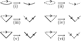
Figure 2: Homotopy moves.

We now describe the means of performing the homotopy in a way that controls filling length. Repeatedly apply the following four steps:

1. 1-cell collapse (see section 2 above),

2. moves (i) and (ii): bi-gon collapse,

3. moves (iii) and (iv),

4. moves (v) and (vi) in accordance with logarithmic shelling.

The first step in the list that is available is performed, and then we return to the start of the list. Repeating this, the boundary loop of $\mathcal{D}_{i}$ will eventually be reduced to the constant loop at the base point $x_{0}$.

The means by which we use logarithmic shelling to choose which 2-cell to collapse when performing step 4 requires some explanation. The result of cutting $\mathcal{D}_{i}$ along $\mathcal{T}$ and removing 2-cells of the type encountered in (i),(ii),(iii), and (iv) of Figure 2, is illustrated in Figure 3. Taking the dual gives a rooted tree of the form discussed in Section 3. The 2-cell to be pushed across is chosen in accordance with the process of logarithmic shelling of rooted trees discussed there. The number of nodes in the tree is at most $A$ and so by Corollary 1 the visibility number is at most $\log_{2}(A+1)+1$.

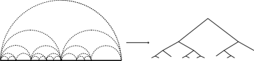
Figure 3: The shelling tree of $\mathcal{D}_{i}$.

It remains to explain how performing the elementary homotopy as described above leads to the required bound on $h_{0}$. Consider the situation when the next step to be applied is number 4. The visibility number associated to the dual tree described above is at most $\log_{2}(A+1)+1$. The homotopy loop includes at most $\log_{2}(A+1)+1$ edges of the type occurring in move (vi). These are separated by paths in $\mathcal{T}$ of length at most $2D$. The loop is closed by another path in $\mathcal{T}$ again of length at most $2D$. So this loop has length at most:

$$\log_{2}(A+1)+1+2D\log_{2}(A+1)+2D=(2D+1)(\log_{2}(A+1)+1).$$

Now applying move (v) or (vi) increases the length of the loop by 1, creating two new channels where moves (i), (ii), (iii) and (iv) may be performed. Consider then applying steps 1, 2 and 3. Step 1 can only decrease the length, and step 2 leaves it unchanged. Step 3 can be applied at most $2D$ times in each of the two channels. Thus the increase in length before step 4 is next applied is at most $1+4D$. This gives bound

$$\text{FL}(\mathcal{D}_{i})\leq(2D+1)(\log_{2}(A+1)+1)+4D+1.$$

Combining this with the inequality (2) we have our result.

5 Examples

In this section we provide a proof for the assertion made in section 2 about an AD-pair for a group with a polynomial isoperimetric function. We then give applications of Theorem 1 to particular classes of groups, and we conclude with a discussion of an open question.

Proposition 3

Let $\Gamma$ be a group admitting a polynomial isoperimetric function of degree $r\geq 2$. Then up to a common multiplicative constant $(x^{r},x^{r-1})$ is an AD-pair for $\Gamma$.

Papasoglu gives this result for $r=2$ in [11, page 799]. It requires a small generalisation of his argument to obtain the result for all $r\geq 2$, as follows. (See also [9, page 100].)

We will make use of some of definitions. Let the radius of a van Kampen diagram $\mathcal{D}$ to be

$$\text{Rad}(\mathcal{D}):=\max\left\{d(v,\partial\mathcal{D}):v\text{ is a vertex of }\mathcal{D}\right\},$$

where $d(v,\partial\mathcal{D})$ is the combinatorial distance in the 1-skeleton.

For a subcomplex $K$ of $\mathcal{D}$ define $\text{star}(K)$ to be the union of closed 2-cells meeting $K$. Define $\text{star}_{i}(K)$ to be the $i$-th iterate of the star operation for $i\geq 1$; by convention $\text{star}_{0}(K)=K$. So if $\Gamma$ is triangularly presented then the 0-cells in $\text{star}_{i}(\partial\mathcal{D})$ are precisely those a distance at most $i$ from $\partial D$.

The substance of Proposition 3 is in the following lemma.

Lemma 2

Suppose $\Gamma=\left<\mathcal{A}\left|\mathcal{R}\right.\right>$ is triangularly presented (see the paragraph following Proposition 2) and that $\mathcal{R}$ includes all null-homotopic words of length at most 3. Suppose further that there is $M>0$ such that $f_{0}(n)\leq Mn^{r}$ for all $n$. Then for all null-homotopic $w$ we have $\text{Rad}(\mathcal{D})\leq 12M\left|w\right|^{r-1}$, where $\mathcal{D}$ is a minimal area van Kampen diagram for $w$.

As discussed in section 4, a change of finite presentation induces a $\simeq$-equivalence on isoperimetric and isodiametric functions. Note that there are only finitely many words of length at most 3 in a finitely presented group. Also observe that adding $n/2$ is sufficient to obtain a diameter bound from a radius bound. Thus this lemma is sufficient to prove Proposition 3.

Proof of Lemma 2. We proceed by induction on $n$. For $n\leq 3$ the result follows from our insistence that $\mathcal{R}$ includes all null-homotopic words of length at most 3.

For the induction step suppose $w$ is null-homotopic and $\left|w\right|=n$. Let $\mathcal{D}$ be a minimal area van Kampen diagram for $w$. Let $N_{i}:=\text{star}_{i}(\partial\mathcal{D})$. Let $c_{i}:=\partial N_{i}-\partial\mathcal{D}$, which is the union of simple closed curves any two of which meet at one point or not at all (note that $c_{0}=\partial(\text{star}_{0}(\partial D))-\partial D$, which is empty).

Now $\text{Area}(N_{i+1})-\text{Area}(N_{i})\geq l(c_{i})/3$ because every 1-cell of $c_{i}$ lies in the boundary of some 2-cell in $N_{i+1}-N_{i}$.

For all $i$,

$$\text{Area}(\mathcal{D})\geq\text{Area}(N_{i+1})\geq l(c_{i})/3+l(c_{i-1})/3+\cdots+l(c_{0})/3.$$

Thus if $l(c_{i})>n/2$ for all $i\leq 6Mn^{r-1}$ we get a contradiction of the area bound $Mn^{r}$ for $\mathcal{D}$. So for some $i\leq 6Mn^{r-1}$ we find $l(c_{i})\leq n/2$. We can appeal to the inductive hypothesis to learn that the diagrams enclosed by the simple closed curves constituting $c_{i}$ have radius at most $12M(n/2)^{r-1}\leq 6Mn^{r-1}$.

So a vertex $v$ of $\mathcal{D}$ either lies in $N_{i}$, in which case $d(v,\partial\mathcal{D})\leq 6Mn^{r-1}$, or is in a diagram enclosed by one of the simple closed curves $c$ of $c_{i}$ . In the latter case $d(v,\partial\mathcal{D})\leq d(v,c)+d(c,\partial\mathcal{D})\leq 12Mn^{r-1}$ as required, thus completing the proof of the lemma.

We now give some applications of our main theorem to particular classes of groups.

Example Polynomial isoperimetric function. If the finitely presented group $\Gamma$ admits a polynomial isoperimetric function of degree $r\geq 2$, it follows from Theorem 1 and Proposition 3 above that $h_{0}(n)\preceq n^{r-1}\log(n+1)$. This contrasts with the inequality $h_{0}\preceq f_{0}$ in section 2 Example 1.

Example Bridson’s Groups $\Gamma_{m}$ (see section 3 Example 5). These have AD-pairs $(x^{2m+1},x^{m})$ and so Theorem 1 gives us bounds of $x^{m}\log x$ on their filling length functions, which is a significant improvement on the bounds $x^{2m+1}$ obtained from the inequality $h_{0}\preceq f_{0}$.

Open question In connection with the double exponential bound quoted in section 2 Example 3, it is an open problem, to our knowledge first raised by John Stallings, whether there is always a simple exponential bound $f_{0}\preceq\exp g_{0}$. It is natural then to ask whether there is always an AD-pair of the form $(\exp g_{0},g_{0})$. (This adds the requirement that the $\exp g_{0}$ bound on $f_{0}$ is always realisable on the same van Kampen diagram as $g_{0}$.) Our main theorem gives a necessary condition that this be true, namely that $h_{0}\preceq{g_{0}}^{2}$.

We shall now make some observations relevant to the single exponential question just stated.

Proposition 4

If $\mathcal{P}$ is a finite presentation, then for all integers $N\geq 3$ there exists $C(N)>0$ such that for all van Kampen diagrams $\mathcal{D}$ in $\mathcal{P}$ all of whose vertices have valence at most $N$ one has

1. $Area(\mathcal{D})\leq N^{Diam(\mathcal{D})+1}-1$, and

2. $FL(\mathcal{D})\leq C(N)\cdot Diam(\mathcal{D})^{2}+n+1$.

Proof. The number of vertices at a given distance $i$ from the base point is at most $N(N-1)^{i-1}$, so it follows that the number of geometric edges $E(\mathcal{D})$ satisfies $E(\mathcal{D})\leq N+N^{2}+\cdots+N^{D}<\frac{N^{D+1}-1}{N-1}$, where $D=Diam(\mathcal{D})$. Since each edge is incident with at most 2 faces, we get $Area(\mathcal{D})\leq 2\frac{N^{D+1}-1}{N-1}\leq N^{D+1}-1$, giving the first conclusion of the proposition.

¿From Proposition 2 it follows that $FL(\mathcal{D})\leq(2D+1)(D+1)\log_{2}(N)+4D+1+n=C(N)D^{2}+n+1$, where $C(N)$ depends only on $N$, proving the second conclusion.

Corollary 2

For every finite presentation $\mathcal{P}$ there is a constant $C>0$ such that if $\mathcal{D}$ is an immersed topological disc diagram in $\mathcal{P}$, then $FL(\mathcal{D})\leq C\cdot\text{Diam}(\mathcal{D})^{2}+n+1$.

Proof. Since $\mathcal{D}$ is immersed, the valence of a vertex $v$ is at most the number of edges incident at a vertex of the Cayley graph, namely, twice the number of generators of $\mathcal{P}$. The corollary follows from the second conclusion of the proposition.

Remark. Gromov observed in [9] 5C that if $h_{0}\preceq g_{0}$, then it follows that $f_{0}\preceq\exp g_{0}$; one sees this as a consequence of section 2 Example 3 above. We do not know an example from finitely presented groups where $h_{0}\preceq g_{0}$ fails; however it is shown in [5] that this can fail in a simply connected Riemannian context.

Steve Gersten	Tim Riley
Mathematics Department	Mathematical Institute
University of Utah	24-29 St Giles
Salt Lake City	Oxford
UT 84112	OX1 3LB
USA	UK
E-mail: gersten@math.utah.edu	E-mail: rileyt@maths.ox.ac.uk

References

- [1] M. Bridson. Asymptotic cones and polynomial isoperimetric inequalities. Topology, 38(3):543–554, 1999.
- [2] M. Bridson and A. Haefliger. Metric Spaces of Non-positive Curvature. Number 319 in Grundlehren der mathematischen Wissenschaften. Springer Verlag, 1999.
- [3] D. E. Cohen. Isoperimetric and isodiametric inequalities for group presentations. Int. J. of Alg. and Comp., 1(3):315–320, 1991.
- [4] D. B. A. Epstein, J. W. Cannon, S. F. Holt, S. V. F. Levy, M. S. Paterson, and W. P. Thurston. Word Processing in Groups. Jones and Bartlett, 1992.
- [5] S. Frankel and M. Katz. The Morse landscape of a Riemannian disc. Ann. Inst. Fourier, Grenoble, 43(2):503–507, 1993.
- [6] S. Gersten. The double exponential theorem for isoperimetric and isodiametric functions. Int. J. of Alg. and Comp., 1(3):321–327, 1991.
- [7] S. Gersten. Isoperimetric and isodiametric functions. In G. Niblo and M. Roller, editors, Geometric group theory II, number 182 in LMS lecture notes. Camb. Univ. Press, 1993.
- [8] S. Gersten. Asynchronously automatic groups. In Charney, Davis, and Shapiro, editors, Geometric group theory, pages 121–133. de Gruyter, 1995.
- [9] M. Gromov. Asymptotic invariants of infinite groups. In G. Niblo and M. Roller, editors, Geometric group theory II, number 182 in LMS lecture notes. Camb. Univ. Press, 1993.
- [10] R. C. Lyndon and P. E. Schupp. Combinatorial Group Theory. Springer Verlag, 1977.
- [11] P. Papasoglu. On the asymptotic invariants of groups satisfying a quadratic isoperimetric inequality. J. Diff. Geom., 44:789–806, 1996.