Kashaev’s invariant and the volume of a hyperbolic knot after Y. Yokota

Abstract.

I follow Y. Yokota to explain how to obtain a tetrahedron decomposition of the complement of a hyperbolic knot and compare it with the asymptotic behavior of Kashaev’s link invariant using the figure-eight knot as an example.

1. Introduction

In [1] R. Kashaev introduced a link invariant by using the quantum dilogarithm and after some concrete calculations for the knots $4_{1}$, $5_{2}$, and $6_{1}$, he conjectured in [2] the asymptotic behavior of his invariant determines the hyperbolic volume for hyperbolic links. More precisely his conjecture is as follows. For an integer $N\geq 2$ let $\langle{L}\rangle_{N}$ be the Kashaev invariant of a link $L$.

Conjecture 1.1 (Kashaev).

If $L$ is hyperbolic, i.e. $S^{3}\setminus{L}$ has a complete hyperbolic structure, then

$$2\pi\lim_{N\to\infty}\frac{\log\left|\langle{L}\rangle_{N}\right|}{N}=\operatorname{Vol}(L),$$

where $\operatorname{Vol}(L)$ is the volume of $S^{3}\setminus{L}$.

On the other hand in [3], J. Murakami and I proved that Kashaev’s invariant coincides with a colored Jones polynomial evaluated at a root of unity. By using this Y. Yokota, following D. Thurston [7], considered a tetrahedron decomposition corresponding to the $R$-matrix used to define colored Jones polynomials and showed that at least for a concrete example, the knot $6_{2}$, this decomposition gives a nice and constructive proof for Kashaev’s conjecture [11] (he also mentioned that this seems work well for other knots; especially for alternating knots). Several computations (without tetrahedron decompositions) were made in [4] and the conjecture was also confirmed for the knots $6_{3}$, $7_{2}$, and $8_{9}$, and for the Whitehead link. (In [4] a relation between the asymptotic behavior of the Kashaev invariant and the Chern–Simons invariant is also mentioned.)

After that Yokota used Kashaev’s original $R$-matrix and found another tetrahedron decomposition of a hyperbolic knot complement fit for the asymptotic behavior of Kashaev’s invariant [9] (see also [10]). This gives simpler decompositions and seems to work much better including non-alternating knots.

This is an expository note to describe Yokota’s method explaining beautiful harmony of Kashaev’s invariants and hyperbolic structures, putting special emphasis on the figure-eight knot.

Acknowledgments.

Part of this work was prepared for a series of lectures at Chiba University in July, 2000. I would like to thank K. Kuga for giving me the opportunity to give lectures there. Thanks are also due to J. Murakami, M. Okamoto, T. Takata and Y. Yokota for helpful discussions.

2. Algebra

In this section I describe Kashaev’s link invariant [1] following Yokota. We fix an integer $N\geq 2$ and put $q=\exp\left(2\pi\sqrt{-1}/N\right)$. Put $(x)_{n}=\prod_{k=1}^{n}(1-x^{k})$ for $n\geq 0$. For integers $0{\leq}k,l,m,n{\leq}N-1$ we put

$$\theta\!\left(\begin{smallmatrix}k&n\\ l&m\end{smallmatrix}\right)=\begin{cases}1\;&\text{if ${l}\neq{m}$ and $q^{k},q^{l},q^{m},q^{n}$ are on the unit circle counterclockwise}\\ &\hfill\text{(other pairs may be the same)},\\ 0\;&\text{otherwise}.\end{cases}$$

Note that $\theta\!\left(\begin{smallmatrix}k&n\\ l&m\end{smallmatrix}\right)=1$ if and only if

$${k}\leq{l}<{m}\leq{n},\quad{n}\leq{k}\leq{l}<{m},\quad{m}\leq{n}\leq{k}\leq{l}\;(m<l),\;\text{or}\quad{l}<{m}\leq{n}\leq{k}.$$

For an integer $x$, we denote by $[x]\in\{0,1,2,\dots,N-1\}$ the residue modulo $N$.

Now Kashaev’s $R$-matrix $R=\left(R_{l,m}^{k,n}\right)$ is an $N^{2}\times N^{2}$-matrix given by

$$R_{l,m}^{k,n}=\frac{Nq^{1-(l-n+1)(m-k)}\theta\!\left(\begin{smallmatrix}k&n\\ l&m\end{smallmatrix}\right)}{(q)_{[m-l-1]}(q^{-1})_{[n-m]}(q)_{[k-n]}(q^{-1})_{[l-k]}}$$

and

$$\left(R^{-1}\right)_{l,m}^{k,n}=\frac{Nq^{-1+(m-k-1)(l-n)}\theta\!\left(\begin{smallmatrix}k&n\\ l&m\end{smallmatrix}\right)}{(q^{-1})_{[m-l-1]}(q)_{[n-m]}(q^{-1})_{[k-n]}(q)_{[l-k]}}.$$

Let $\mu$ be an $N\times N$-matrix with $\mu_{l}^{k}=-\delta_{k,l+1}q^{1/2}$, where $\delta_{i,j}$ is Kronecker’s delta. Then $(R,\mu,-q^{1/2},1)$ is an enhanced Yang–Baxter operator [8], i.e. the following equalities hold. (See [3] for a proof.)

Proposition 2.1.

$$\left({R}\otimes{id}_{\mathbb{C}^{N}}\right)\left({id}_{\mathbb{C}^{N}}\otimes{R}\right)\left({R}\otimes{id}_{\mathbb{C}^{N}}\right)=\left({id}_{\mathbb{C}^{N}}\otimes{R}\right)\left({R}\otimes{id}_{\mathbb{C}^{N}}\right)\left({id}_{\mathbb{C}^{N}}\otimes{R}\right),$$

$$\left(\mu\otimes\mu\right)R=R\left(\mu\otimes\mu\right),$$

$$\sum_{m=0}^{N-1}\left(R^{\pm 1}({id}_{\mathbb{C}^{N}}\otimes\mu)\right)_{lm}^{km}=\left(-q^{1/2}\right)^{\pm 1}\delta_{k,l}$$

with ${id}_{\mathbb{C}^{N}}$ the identity on $\mathbb{C}^{N}$.

Now I will describe how to calculate Kashaev’s invariant for knots using this enhanced Yang-Baxter operator.

First we present a knot in a $(1,1)$-tangle formula so that the string comes from above and goes down and at each crossing both arcs also go down. We decompose the string into edges so that at each crossing four edges meet and at each maximum/minimum where the string go from the left to the right two edges meet. See Figure 2.1 for example. A labeling is an assignment of an element in $\{0,1,2,\dots,N-1\}$ to each edge. Here we assign $0$ to the edge from the starting point and to the edge to the end point. We call the number assigned to an edge its label. Given a labeling we assign the following quantities to crossings and maxima/minima:

$$\raisebox{-14.22636pt}{\begin{picture}(10.0,10.0)\put(10.0,10.0){\vector(-1,-1){10.0}} \put(6.0,4.0){\vector(1,-1){4.0}} \put(4.0,6.0){\line(-1,1){4.0}} \put(0.0,10.0){\makebox(0.0,0.0)[br]{$k$}}\put(10.0,10.0){\makebox(0.0,0.0)[bl]{$n$}} \put(0.0,0.0){\makebox(0.0,0.0)[tr]{$l$}}\put(10.0,0.0){\makebox(0.0,0.0)[tl]{$m$}} \end{picture}}\,:\,R_{lm}^{kn},\qquad\raisebox{-14.22636pt}{\begin{picture}(10.0,10.0)\put(0.0,10.0){\vector(1,-1){10.0}} \put(10.0,10.0){\line(-1,-1){4.0}} \put(4.0,4.0){\vector(-1,-1){4.0}} \put(0.0,10.0){\makebox(0.0,0.0)[br]{$k$}}\put(10.0,10.0){\makebox(0.0,0.0)[bl]{$n$}} \put(0.0,0.0){\makebox(0.0,0.0)[tr]{$l$}}\put(10.0,0.0){\makebox(0.0,0.0)[tl]{$m$}} \end{picture}}\,:\,\left(R^{-1}\right)_{lm}^{kn},\qquad\raisebox{-7.11317pt}{\begin{picture}(10.0,5.0)\qbezier(0.0,5.0)(0.0,0.0)(5.0,0.0)\qbezier(5.0,0.0)(10.0,0.0)(10.0,5.0)\put(5.0,-1.0){\line(0,1){2.0}} \put(9.0,5.5){\vector(0,1){0.0}} \put(1.0,1.0){\makebox(0.0,0.0)[tr]{$k$}} \put(9.0,1.0){\makebox(0.0,0.0)[tl]{$l$}} \end{picture}}\,:\,\mu_{l}^{k},\qquad\raisebox{-7.11317pt}{\begin{picture}(10.0,5.0)\qbezier(0.0,0.0)(0.0,5.0)(5.0,5.0)\qbezier(5.0,5.0)(10.0,5.0)(10.0,0.0)\put(5.0,4.0){\line(0,1){2.0}} \put(10.1,-0.5){\vector(0,-1){0.0}} \put(1.0,4.0){\makebox(0.0,0.0)[br]{$k$}} \put(9.0,4.0){\makebox(0.0,0.0)[bl]{$l$}} \end{picture}}\,:\,\left(\mu^{-1}\right)_{l}^{k}.$$

The weight for a labeling is the product of all the quantities above. Then the Kashaev invariant $\langle{K}\rangle_{N}$ of a knot $K$ is defined to be the sum of all the weights up to some power of $q$ (which does not matter in our case), where the summation runs over all the labelings.

If four edges meeting at a crossing are labeled $k$, $l$, $m$ and $n$ as above, we call $[n-m]$, $[k-n]$, $[l-k]$ and $[m-l-1]$ the angles between the adjacent edges. Then we have the following proposition.

Proposition 2.2 ([9, Proposition 2]).

The weight for a labeling vanishes unless all of the following conditions are satisfied. For a proof see [9].

1. the sum of the angles around any crossing is $N-1$.

2. the sum of the angles contained in any bounded region is $N-1$.

3. any angle in any of the two unbounded regions is zero.

We will calculate the Kashaev invariant for the figure-eight knot.

From Proposition 2.2 (3), we can assume that labels are as in Figure 2.1.

Figure 2.1. Figure-eight knot with a labeling.

Then the Kashaev invariant $\langle{4_{1}}\rangle_{N}$ is

$$\sum_{j=0}^{N-1}\sum_{k\in[0,j-1]}\sum_{i\in[1,j]}\left(R^{-1}\right)_{0,i}^{0,0}\left(R^{-1}\right)_{0,1}^{j,i}R_{N-1,0}^{\phantom{N}k\phantom{1},0}R_{k,j}^{0,0}\left(\mu^{-1}\right)_{N-1}^{0}\mu_{1}^{0}$$

$$=N^{4}\sum_{j=0}^{N-1}\sum_{k\in[0,j-1]}\sum_{i\in[1,j]}\frac{q^{-1}}{(q^{-1})_{[i-1]}(q)_{[-i]}}\times\frac{q^{-1+(-j)(-i)}}{(q)_{[i-1]}(q^{-1})_{[j-i]}(q)_{[-j]}}$$

$$\phantom{N^{4}\sum_{j=0}^{N-1}\sum_{k\in[0,j-1]}\sum_{i\in[1,j]}}\times\frac{q^{1-(N)(-k)}}{(q)_{[k]}(q^{-1})_{[-k-1]}}\times\frac{q^{1-(k+1)j}}{(q)_{[j-k-1]}(q^{-1})_{[-j]}(q^{-1})_{[k]}}$$

$$=N^{2}\sum_{j=0}^{N-1}\frac{q^{-j}}{(q)_{[-j]}(q^{-1})_{[-j]}}\sum_{k\in[0,j-1]}\frac{q^{-kj}}{(q)_{[j-k-1]}(q^{-1})_{[k]}}\sum_{i\in[1,j]}\frac{q^{ij}}{(q)_{[i-1]}(q^{-1})_{[j-i]}}$$

up to some power of $q$, since $(q^{-1})_{[i-1]}(q)_{[-i]}=(q^{-1})_{i-1}(q)_{N-i}=\dfrac{N}{(q)_{N-i}}(q)_{N-i}=N$ and $(q)_{[k]}(q^{-1})_{[-k-1]}=(q)_{k}\dfrac{N}{(q)_{k}}=N$. Here $a\in[b,c]$ means that $q^{b}$, $q^{a}$, and $q^{c}$ are on the unit circle counterclockwise (any pair may be the same). Note that $a\in[b,c]$ if and only if $[a-b]+[c-a]=[c-b]$.

From the lemma below we have

$$\langle{4_{1}}\rangle_{N} =N^{2}\sum_{j=0}^{N-1}\frac{(-1)^{[j-1]}q^{-j-([j-1]+1)([j-1]-2j)/2}}{(q)_{[-j]}(q^{-1})_{[-j]}}\sum_{k\in[0,j-1]}\frac{q^{-kj}}{(q)_{[j-k-1]}(q^{-1})_{[k]}}$$

$$=N^{2}\sum_{j=0}^{N-1}\frac{1}{(q)_{[-j]}(q^{-1})_{[-j]}}$$

$$=\sum_{j=0}^{N-1}(q)_{[N-1+j]}(q^{-1})_{[N-1+j]}$$

$$=\sum_{j=0}^{N-1}(q)_{j}(q^{-1})_{j}.$$

Note that the final formula coincides with Kashaev’s [2, (2.2)].

The following lemma is a key to reduce the summations of the Kashaev’s invariant.

Lemma 2.3 (Yokota’s version of [3, Lemma 3.2]).

Let $0\leq{k},{l},{m}\leq{N-1}$ be integers. Then

$$\sum_{k\in[l,m]}\frac{q^{-(m-l+1)k}}{(q)_{[m-k]}(q^{-1})_{[k-l]}}=(-1)^{[m-l]}q^{([m-l]+1)([m-l]-2m)/2}.$$

Proof.

We use the following equality [3, Lemma 3.2].

$$\begin{split}&\sum_{i=0}^{N-1-\alpha}\frac{q^{(\beta-\alpha)i/2}}{(q)_{i}(q^{-1})_{N-1-\alpha-i}}\\ &\quad=\frac{(-1)^{N-1-\alpha}q^{-N(N-1)/2-\beta(\alpha+1)/2}}{N}\frac{(q)_{\alpha}(q)_{N-1-\alpha+[(\alpha-\beta)/2]}}{(q)_{[(\alpha-\beta)/2]}}.\end{split}$$

To prove the lemma, we put $\beta=-\alpha$. Then we have

$$\sum_{i=0}^{N-1-\alpha}\frac{q^{-\alpha i}}{(q)_{i}(q^{-1})_{N-\alpha-i-1}}=(-1)^{N-1-\alpha}q^{-N(N-1)/2+\alpha(\alpha+1)/2}.$$

Putting $i=[m-k]$ and $N-\alpha-1=[m-l]$, the conclusion follows. ∎

3. Geometry

In this section I will describe how to decompose a knot complement $S^{3}\setminus{K}$ into ideal topological tetrahedra and how these define hyperbolic structure when $K$ is the figure-eight knot. Here ‘ideal’ means that each vertex is at the cusp (the infinite point corresponding to $K$). (That is, all vertices of the tetrahedra meet at a point, and the complement of the regular neighborhood of the point is $S^{3}\setminus{K}$.)

Fix a knot diagram throughout.

3.1. Ideal tetrahedron decomposition of $S^{3}\setminus({K\cup\text{two points}})$

We will decompose $S^{3}\setminus({K\cup\text{two points}})$ into tetrahedra so that all the vertices are either on $K$ or on the two points outside $K$.

First we put an octahedron ${\rm E}_{i}$-${\rm A}_{i}{\rm B}_{i}{\rm C}_{i}{\rm D}_{i}$-${\rm F}_{i}$ at the $i$th crossing of the knot diagram so that ${\rm E}_{i}{\rm F}_{i}$ is perpendicular to the plane, that ${\rm E}_{i}$ and ${\rm F}_{i}$ touch the over-crossing point and the under-crossing point respectively, and that ${\rm A}_{i}$, ${\rm B}_{i}$, ${\rm C}_{i}$, and ${\rm D}_{i}$ are to the northeast, northwest, southwest, and southeast, respectively. (see Figures 3.1 and 3.3). We call this the $i$th octahedron.

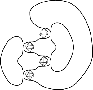
Figure 3.1. Put octahedra at crossings.

We decompose each octahedron into four tetrahedra as shown in Figure 3.2. (For the figure-eight knot, we now have 16 tetrahedra.) We name each vertex of the tetrahedra as in Figure 3.2. (Here we drop subscriptions.)

Figure 3.2. Decompose an octahedron into four tetrahedra.

We deform an octahedron attached to a positive crossing as follows. We pull the vertices ${\rm B}$ and ${\rm D}$ upward and identify the edge ${\rm EB}$ with the edge ${\rm ED}$. Similarly we pull the vertices ${\rm A}$ and ${\rm C}$ downward and identify the edge ${\rm FA}$ with the edge ${\rm FC}$. (See Figure 3.3.)

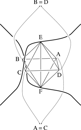
Figure 3.3. Pull the pairs of vertices to $\pm\infty$.

Now the resulting twisted octahedron consists of four twisted tetrahedra (Figure 3.4).

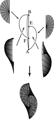
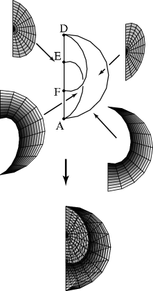
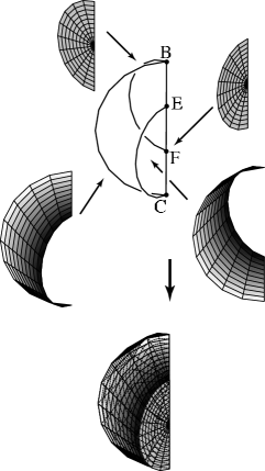
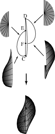
Figure 3.4. Twisted tetrahedra.

The surface of a twisted octahedron consists of four leaves made from $\triangle{b^{+}}{b^{r}}{b^{l}}\cup\triangle{c^{+}}{c^{r}}{c^{l}}$, $\triangle{c^{-}}{c^{l}}{c^{r}}\cup\triangle{d^{-}}{d^{l}}{d^{r}}$, $\triangle{d^{+}}{d^{r}}{d^{l}}\cup\triangle{a^{+}}{a^{r}}{a^{l}}$, and $\triangle{a^{-}}{a^{l}}{a^{r}}\cup\triangle{b^{-}}{b^{l}}{b^{r}}$, which we will call Leaf $\gamma$, Leaf $\delta$, Leaf $\alpha$, and Leaf $\beta$, respectively (Figure 3.5).

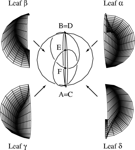
Figure 3.5. A twisted octahedron and its four leaves.

Now this twisted octahedron and the near positive crossing look like Figure 3.6.

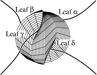
Figure 3.6. A twisted octahedron and a crossing.

For an octahedron attached to a negative crossing we deform it similarly. We pull the vertices ${\rm B}$ and ${\rm D}$ downward, and ${\rm A}$ and ${\rm C}$ upward to identify the edge ${\rm EB}$ with the edge ${\rm ED}$, and the edge ${\rm FA}$ with the edge ${\rm FC}$. In this case Leaf $\alpha$ is made from $\triangle{d^{-}}{d^{l}}{d^{r}}$ and $\triangle{a^{-}}{a^{l}}{a^{r}}$, and Leaves $\beta$, $\gamma$, and $\delta$ are from $\triangle{a^{+}}{a^{r}}{a^{l}}$ and $\triangle{b^{+}}{b^{r}}{b^{l}}$, $\triangle{b^{-}}{b^{l}}{b^{r}}$ and $\triangle{c^{-}}{c^{l}}{c^{r}}$, and $\triangle{c^{+}}{c^{r}}{c^{l}}$ and $\triangle{d^{+}}{d^{r}}{d^{l}}$, respectively.

Now the whole picture for the figure-eight knot is as shown in Figure 3.7.

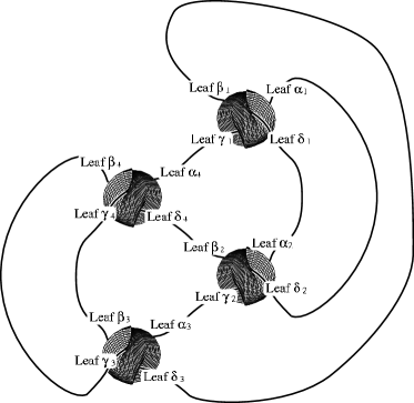
Figure 3.7. Figure-eight knot with twisted octahedra.

Next we identify two leaves facing each other along an arc by thickening the octahedra and shortening the arc. For the figure-eight knot case, we identify Leaves $\delta_{1}$ and $\alpha_{2}$, $\gamma_{2}$ and $\alpha_{3}$, $\gamma_{3}$ and $\beta_{4}$, $\delta_{4}$ and $\beta_{2}$, $\delta_{2}$ and $\alpha_{1}$, $\gamma_{1}$ and $\alpha_{4}$, $\gamma_{4}$ and $\beta_{3}$, and $\delta_{3}$ and $\beta_{1}$. Then the eight vertices ${\rm A_{1}}$, ${\rm C_{1}}$, ${\rm A_{2}}$, ${\rm C_{2}}$, ${\rm B_{3}}$, ${\rm D_{3}}$, ${\rm B_{4}}$, and ${\rm D_{4}}$ are identified. We call the resulting vertex $+\infty$. Similarly the eight vertices ${\rm B_{1}}$, ${\rm D_{1}}$, ${\rm B_{2}}$, ${\rm D_{2}}$, ${\rm A_{3}}$, ${\rm C_{3}}$, ${\rm A_{4}}$, and ${\rm C_{4}}$ are identified with the new vertex $-\infty$. Moreover the other eight vertices $E_{1},F_{1},\dots,E_{4},F_{4}$ are also identified, which we call ${\rm G}$.

Now we have an ideal tetrahedron decomposition of $S^{3}\setminus({K\cup\pm\infty})$ with three ideal vertices. The boundary torus of the regular neighborhood of ${\rm G}$ and the boundary spheres of the regular neighborhoods of $\pm\infty$ look like Figures 3.8, 3.9, and 3.10 respectively if $K$ is the figure-eight knot. Note that we always look at boundaries from the outside.

Figure 3.8. Boundary of the regular neighborhood of ${\rm G}$. (The wavy lines, the dotted lines, and the sidelines are identified respectively.)

Figure 3.9. Boundaries of the regular neighborhoods of ${\rm A_{1}=C_{1}}$, ${\rm A_{2}=C_{2}}$, ${\rm B_{3}=D_{3}}$, and ${\rm B_{4}=D_{4}}$ together with knot diagram before thickening the twisted octahedra viewed from the top (left). Boundary of the regular neighborhood of $+\infty$ (right).

Figure 3.10. Boundaries of the regular neighborhoods of ${\rm B_{1}=D_{1}}$, ${\rm B_{2}=D_{2}}$, ${\rm A_{3}=C_{3}}$, and ${\rm A_{4}=C_{4}}$ together with knot diagram before thickening the twisted octahedra viewed from the bottom (left). Boundary of the regular neighborhood of $-\infty$ (right).

3.2. Ideal tetrahedron decomposition of $S^{3}\setminus{K}$

We will deform the ideal tetrahedron decomposition of $S^{3}\setminus({K\cup\pm\infty})$ given above to obtain an ideal tetrahedron decomposition of $S^{3}\setminus{K}$.

To do this we collapse Leaf $\beta_{1}$ (= Leaf $\delta_{3}$) into the point $G=E_{1}=F_{1}=\dots=E_{4}=F_{4}$ and extend this collapsing over the other tetrahedra linearly. Note that this leaf corresponds to the broken point of the knot diagram to make it a $(1,1)$-tangle in § 2.

I will show how octahedra will collapse.

In the first octahedron ${\rm E_{1}}$-${\rm A_{1}B_{1}C_{1}D_{1}}$-${\rm F_{1}}$, there are two faces $\triangle{a^{+}_{1}}{a^{r}_{1}}{a^{l}_{1}}$ and $\triangle{b^{+}_{1}}{b^{r}_{1}}{b^{l}_{1}}$ which make Leaf $\beta_{1}$. Therefore the tetrahedron ${\rm F_{1}E_{1}A_{1}B_{1}}$ and ${\rm F_{1}E_{1}B_{1}C_{1}}$ (they are the cones over $\triangle{a^{+}_{1}}{a^{r}_{1}}{a^{l}_{1}}$ and $\triangle{b^{+}_{1}}{b^{r}_{1}}{b^{l}_{1}}$ with ${\rm F_{1}}$) are collapsed to edges and so three edges ${\rm F_{1}A_{1}}$, ${\rm F_{1}B_{1}}$ and ${\rm F_{1}C_{1}}$ are identified with the edge ${\rm F_{1}E_{1}}$. The tetrahedron ${\rm F_{1}E_{1}C_{1}D_{1}}$ and ${\rm F_{1}E_{1}D_{1}A_{1}}$ (they are the joins ${\rm E_{1}C_{1}}*{\rm D_{1}F_{1}}$ and ${\rm E_{1}A_{1}}*{\rm D_{1}F_{1}}$) are collapsed to triangles and so two triangles ${\rm F_{1}D_{1}C_{1}}$ and ${\rm F_{1}A_{1}D_{1}}$ are identified with the triangle ${\rm E_{1}F_{1}D_{1}}$. So the first octahedron is collapsed to the triangle ${\rm F_{1}E_{1}D_{1}}$. See Figure 3.11.

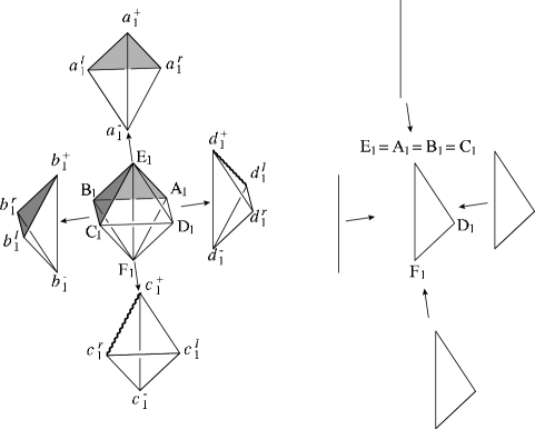
Figure 3.11. The first octahedron is collapsed to the triangle ${\rm F_{1}E_{1}D_{1}}$. (The shaded triangles and the wavy lines are collapsed.)

Similarly the third octahedron is collapsed to the triangle ${\rm F_{3}E_{3}B_{3}}$ since it contains the faces $\triangle{c^{-}_{3}}{c^{l}_{3}}{c^{r}_{3}}$ and $\triangle{d^{-}_{3}}{d^{l}_{3}}{d^{r}_{3}}$ which make Leaf $\delta_{3}$. Here two triangles ${\rm E_{3}B_{3}C_{3}}$ and ${\rm E_{3}A_{3}B_{3}}$ are identified with the triangle ${\rm F_{3}E_{3}B_{3}}$.

On the other hand the edge ${\rm E_{4}C_{4}}$ is identified with the edge ${\rm C_{3}F_{3}}={\rm A_{3}F_{3}}$, which is contained in Leaf $\delta_{3}$. Moreover the edge ${\rm B_{4}A_{4}}$ is identified with the edge ${\rm C_{1}B_{1}}$, which is contained in Leaf $\beta_{1}$. Therefore the fourth octahedron is collapsed to the tetrahedron ${\rm F_{4}E_{4}D_{4}A_{4}}$ as in Figure 3.12. Here the tetrahedron ${\rm F_{4}E_{4}B_{4}C_{4}}$ is collapsed to the triangle ${\rm F_{4}E_{4}B_{4}}$, which is identified with the triangle ${\rm F_{4}E_{4}B_{4}}$. Then the tetrahedron ${\rm F_{4}E_{4}A_{4}B_{4}}$ is collapsed to the triangle ${\rm F_{4}E_{4}A_{4}}$. The tetrahedron ${\rm F_{4}E_{4}C_{4}D_{4}}$ is collapsed to the triangle ${\rm F_{4}E_{4}D_{4}}$.

Figure 3.12. The fourth octahedron is collapsed to the tetrahedron ${\rm F_{4}E_{4}D_{4}A_{4}}$. (The wavy lines are collapsed.)

Similarly the second octahedron is collapsed to the tetrahedron ${\rm F_{2}E_{2}B_{2}C_{2}}$ since two edges ${\rm E_{2}A_{2}}$ and ${\rm C_{2}D_{2}}$ are collapsed to points respectively.

After all only two tetrahedron ${\rm F_{2}E_{2}B_{2}C_{2}}$ and ${\rm F_{4}E_{4}D_{4}A_{4}}$ survive.

Now we want to know the torus boundary of the regular neighborhood of this new vertex. To do that we first look at the regular neighborhood of Leaf $\beta_{1}$ (= Leaf $\delta_{3}$). Figures 3.13 and 3.14 indicate how it appears in the first and the fourth octahedra respectively and how it is collapsed if we collapse the leaf to a point.

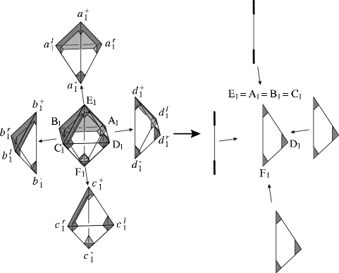
Figure 3.13. The regular neighborhood of Leaf $\beta_{1}$ (= Leaf $\delta_{3}$) in the first octahedron.

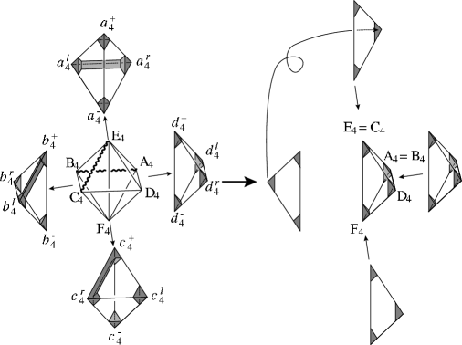
Figure 3.14. The regular neighborhood of Leaf $\beta_{1}$ (= Leaf $\delta_{3}$) in the fourth octahedron.

In the tetrahedron decomposition of $S^{3}\setminus(K\cup\pm\infty)$ the intersections of the regular neighborhood of Leaf $\beta_{1}$ and the boundaries of the (bigger) regular neighborhoods of ${\rm G}$ and $\pm\infty$ look like the shaded regions of Figure 3.15.

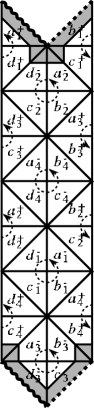
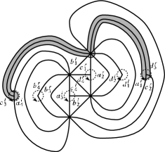
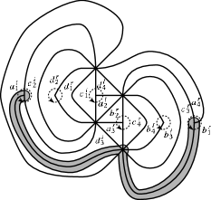
Figure 3.15. The intersections of the regular neighborhood of Leaf $\beta_{1}$ and the boundary of the bigger regular neighborhoods of ${\rm G}$ and $\pm\infty$ are indicated by the shaded regions.

Then we remove the shaded regions and glue the resulting boundaries following the recipe in Figures 3.13 and 3.14, i.e. glue

• $c_{1}^{+}$ and $c_{1}^{r}$, $d_{1}^{+}$ and $d_{1}^{l}$, $a_{3}^{-}$ and $a_{3}^{r}$, $b_{3}^{-}$ and $b_{3}^{l}$, $a_{4}^{r}$ and $a_{4}^{l}$, $b_{4}^{+}$ and $b_{4}^{l}$, $c_{4}^{+}$ and $c_{4}^{r}$, $c_{2}^{r}$ and $c_{2}^{l}$, $d_{2}^{-}$ and $d_{2}^{l}$, and $a_{2}^{-}$ and $a_{2}^{r}$ with quadrangles, and

• $\{a_{1}^{+},a_{1}^{r},a_{1}^{l}\}$, $\{b_{1}^{+},b_{1}^{r},b_{1}^{l}\}$, $\{c_{3}^{-},c_{3}^{r},c_{3}^{l}\}$, $\{d_{3}^{-},d_{3}^{r},d_{3}^{l}\}$ with hexagons.

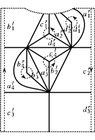
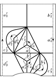
Figure 3.16. Remove the shaded regions in Figure 3.15 and deform the resulting pictures.

Then we have the following pictures of the boundary of the regular neighborhood of $\beta_{1}$ (Figures 3.16 and 3.17).

Figure 3.17. The boundary of the regular neighborhood of $\beta_{1}$.

To collapse it we again follow the recipe in Figures 3.13 and 3.14 and obtain the picture of the boundary of the regular neighborhood of the collapsed $\beta_{1}$. In Figure 3.18 the edges with same numbers are identified.

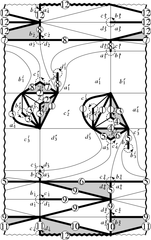
Figure 3.18. The boundary of the regular neighborhood of $\beta_{1}$ after it is collapsed to a point. The edges with same numbers are identified and the shaded regions will survive.

We finally have the triangulation of the cusp torus of $S^{3}\setminus{K}$ (Figure 3.19). In the figure $\lambda$ and $\mu$ denote the latitude (longitude) and the meridian of $K$ respectively.

Figure 3.19. The cusp torus of $S^{3}\setminus{K}$ with the latitude $\lambda$ and the meridian $\mu$.

3.3. Hyperbolicity condition

Now we have a topological ideal tetrahedron decomposition of $S^{3}\setminus{K}$. To introduce a complete hyperbolic structure, we regard each tetrahedron as an ideal hyperbolic tetrahedron parameterized by a complex number with positive imaginary part. This complex parameter $z$ is chosen as follows. First recall that an ideal hyperbolic tetrahedron can be characterized by a Euclidean triangle. (If we consider the upper half space model of the hyperbolic space, then an ideal hyperbolic tetrahedron can be located so that one ideal vertex is at the infinity and the other three are on the $xy$-plane. Then one face of the tetrahedron is in a hemisphere and the other three are in upper half planes perpendicular to the $xy$-plane. Our triangle is the intersection of the three half planes and the $xy$-plane.) If one puts the triangle on the complex plane with two vertices on $0$ and $1$, then the other is on $z$. Note that there are three ways to choose such a parameter (Figure 3.20).

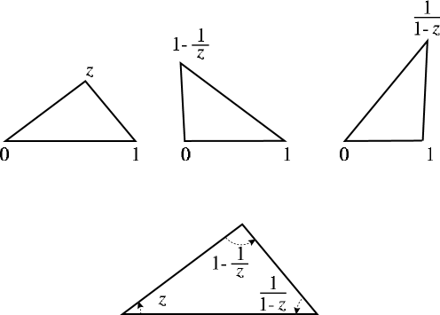
Figure 3.20. Similar triangles parameterized by different complex numbers.

For the tetrahedron with vertex $b_{2}^{\ast}$ we associate $b\in\mathbb{C}$ and that with $d_{4}^{\ast}$ we associate $d\in\mathbb{C}$, where $\ast$ is $+$, $-$, $r$, or $l$. In the cusp torus the triangle labeled $b_{2}^{\ast}$ and $d_{4}^{\ast}$ are similar to the triangles parameterized by $b$ and $d$ respectively for any $\ast$.

It is well known that if the following two conditions are satisfied, then an ideal tetrahedron decomposition parameterized as above defines a hyperbolic structure (more precisely complete hyperbolic structure). (See for example [6, 5].)

1. Consistency condition: at each vertex in the cusp torus, the product of the parameter around the vertex is $1$, and

2. Cusp condition: the products of the parameters along the latitude and the meridian are $1$. Here the parameter of a triangle along a loop is the parameter associated to the small triangle cut by the loop.

Remark 3.1.

The consistency condition means that at each edge of the tetrahedron decomposition the sum of the dihedral angles is equal to $2\pi$. The cusp condition means that the cusp torus is Euclidean.

In our example we have two edges, one connecting $b_{2}^{l}=b_{2}^{-}$ and $b_{2}^{r}=b_{2}^{+}$ and the other connecting $d_{4}^{l}=d_{4}^{+}$ and $d_{4}^{r}=d_{4}^{-}$. So from the consistency condition we have the following two equations since the consistency conditions of two vertices on the torus are the same if they belong to the same edge.

$$b\left(\frac{1}{1-d}\right)b\left(1-\frac{1}{d}\right)\left(1-\frac{1}{b}\right)\left(1-\frac{1}{d}\right) =1,$$

$$d\left(\frac{1}{1-b}\right)\left(\frac{1}{1-d}\right)\left(\frac{1}{1-b}\right)d\left(1-\frac{1}{b}\right) =1.$$

From the cusp condition we have the following two equations.

(3.1) $$\mu :b^{-1}d=1,$$

(3.2) $$\lambda :\left(\frac{1}{1-b}\right)^{-1}d\left(1-\frac{1}{b}\right)^{-1}\left(\frac{1}{1-d}\right)$$

$$\quad\times\left(\frac{1}{1-b}\right)^{-1}d\left(1-\frac{1}{b}\right)^{-1}\left(\frac{1}{1-d}\right)=1.$$

From (3.1) we have $b=d$ and then the rest are all equivalent to $b^{2}-b+1=0$. Since the imaginary part of $b$ should be positive, we have $b=d=\exp(\pi\sqrt{-1}/3)$ and so the two tetrahedra should be regular.

4. Analysis, and Harmony

In §2 we know that if we calculate the Kashaev invariant of the figure-eight knot only the parameter $j$ contributes. Due to Kashaev [2], the asymptotic behavior of $\langle 4_{1}\rangle_{N}$ for large $N$ is

$$\int\exp\left[\frac{N}{2\pi\sqrt{-1}}\left\{-\operatorname{Li}_{2}(z)+\operatorname{Li}_{2}(z^{-1})\right\}\right]\,dz,$$

where $\operatorname{Li}_{2}(z)=-\int_{0}^{z}\log(1-u)/u\,du$ is the dilogarithm function. Note that $z$ corresponds to $q^{j}$ and that $-\operatorname{Li}_{2}(z)$ and $\operatorname{Li}_{2}(z^{-1})$ corresponds to $(q)_{j}$ and $(q^{-1})_{j}$ respectively. We can apply the saddle point method to this integral and know that for large $N$ it is approximated by the value

$$\exp\left[\frac{N\,V(z_{0})}{2\pi\sqrt{-1}}\right]$$

with $V(z):=-\operatorname{Li}_{2}(z)+\operatorname{Li}_{2}(z^{-1})$ and $z_{0}$ satisfies $d\,V(z_{0})/d\,z=0$. Since

$$\frac{d\,V(z)}{d\,z}=\frac{\log(1-z)}{z}+\frac{\log(1-z^{-1})}{z},$$

$z_{0}$ satisfies

(4.1) $$z_{0}^{2}-z_{0}+1=0.$$

Now the Kashaev conjecture follows in this case since $V(z_{0})$ is the volume of the figure-eight knot complement, which is twice the volume of the regular tetrahedron.

On the other hand in §3 we know that only two tetrahedra parameterized by $b$ and $d$ survive. Moreover from the cusp condition these two parameters coincide and satisfy the equation

$$b^{2}-b+1=0,$$

which coincides with (4.1)! Observe that $-\operatorname{Li}_{2}(z)$ corresponds to $(q)_{j-1}=N/(q)_{[-j]}$ which comes from the angle between the edges around the second crossing labeled $0$ and $j$, and $\operatorname{Li}_{2}(z^{-1})$ to $(q^{-1})_{j-1}=N/(q^{-1})_{[-j]}$ which comes from the angle around the fourth crossing between the edges labeled $0$ and $j$.

Yokota proved in [9] similar situations occur for much more general knots including non-alternating knots, showing that for a fixed knot diagram the angles between the surviving labelings of the summation in $\langle{K}\rangle_{N}$ correspond to the surviving dihedral angles in the ideal tetrahedron decomposition and that the partial differential equations defining the saddle point of the integral approximating $\langle{K}\rangle_{N}$ for large $N$ coincide with the hyperbolicity condition. I hope that this note will help the reader to read Yokota’s rather complicated but beautiful paper [9].

References

- [1] R.M. Kashaev, A link invariant from quantum dilogarithm, Modern Phys. Lett. A 10 (1995), no. 19, 1409–1418.
- [2] by same author, The hyperbolic volume of knots from the quantum dilogarithm, Lett. Math. Phys. 39 (1997), no. 3, 269–275.
- [3] H. Murakami and J. Murakami, The colored Jones polynomials and the simplicial volume of a knot, Report No. 20, 1998/99, Institut Mittag-Leffler, arXiv:math.GT/9905075.
- [4] H. Murakami, J. Murakami, M. Okamoto, T. Takata, and Y. Yokota, Kashaev’s conjecture and the Chern–Simons invariants of knots and links, in preparation.
- [5] W.D. Neumann, Combinatorics of triangulations and the Chern-Simons invariant for hyperbolic -manifolds, Topology ’90 (Columbus, OH, 1990) (Berlin), de Gruyter, Berlin, 1992, pp. 243–271.
- [6] W.D. Neumann and D. Zagier, Volumes of hyperbolic three-manifolds, Topology 24 (1985), no. 3, 307–332.
- [7] D. Thurston, Hyperbolic volume and the Jones polynomial, Lecture notes, École d’été de Mathématiques ‘Invariants de nœuds et de variétés de dimension ’, Institut Fourier - UMR 5582 du CNRS et de l’UJF Grenoble (France) du 21 juin au 9 juillet 1999.
- [8] V. G. Turaev, The Yang-Baxter equation and invariants of links, Invent. Math. 92 (1988), 527–553.
- [9] Y. Yokota, On the volume conjecture for hyperbolic knots, in preparation.
- [10] by same author, On the volume conjecture for hyperbolic knots, Proceedings of the 47th Topology Symposium (Inamori Hall, Kagoshima University), July 2000, pp. 38–44.
- [11] by same author, On the volume conjecture of hyperbolic knots, Knot Theory – dedicated to Professor Kunio Murasugi for his 70th birthday (M. Sakuma, ed.), March 2000, pp. 362–367.