Abstract

A toy top is defined as a rotationally symmetric body moving in a constant gravitational field while one point on the symmetry axis is constrained to stay in a horizontal plane. It is an integrable system similar to the Lagrange top. Euler-Poisson equations are derived. Following Felix Klein, the special unitary group $\rm SU(2)$ is used as configuration space and the solution is given in terms of hyperelliptic integrals. The curve traced by the point moving in the horizontal plane is analyzed, and a qualitative classification is achieved. The cases in which the hyperelliptic integrals degenerate to elliptic ones are found and the corresponding solutions are given in terms of Weierstrass elliptic functions.

1 Introduction

The three famous integrable cases of rigid body motion, the tops of Euler, Lagrange and Kowalewsky, have been paramount examples in the theory of integrable systems. The modern algebra-geometric approach, using Lax pairs with a spectral parameter [1], [2] has been applied to all three. It is surprising that the following system appears only sporadically in the literature: A rotationally symmetric rigid body moving in a homogeneous gravitational field with one point on its axis not fixed, but constrained to move in a horizontal plane. Following F. Klein [3, p. 58], we call such a system a toy top.

In many ways, the toy top is similar to Lagrange’s top. It is completely integrable due to the same kind of rotational symmetry. The solution leads to hyperelliptic integrals instead of elliptic ones, but their analytic properties are similar. It seems that Poisson is the first to solve the system [4], using Euler angles. It is treated similarly by E. T. Whittaker [5] and F. Klein [6]. Later, Klein discovered that, as in the case of Lagrange’s top, simpler solutions are obtained when $\rm SU(2)$ is used as configuration space [7], [3].

In this paper we close some gaps in the classical treatment. Following A. I. Bobenko’s and Yu. B. Suris’ treatment of the Lagrange top [8], [9], new equations of motion are derived within the framework of Lagrangian mechanics on Lie groups.

As the toy top moves, its tip traces a curve on the supporting plane. Formulas for this curve are derived and qualitatively different cases are classified.

For certain values of the first integrals, the hyperelliptic integrals appearing in the solution degenerate to elliptic integrals. These cases are classified and the corresponding solutions are given in terms of Weierstrass elliptic functions.

2 Preliminaries

After it is shown how the group of rotations can be considered the configuration space of the toy top, the alternative use of $\rm SU(2)$ is discussed. Finally, Möbius transformations that rotate the Riemann sphere of numbers are discussed for use in chapter 4.

2.1 The group $\rm SU(2)$ as configuration space

The configuration space of the toy top is the direct product of the rotation group with the group of translations in the plane. But since both the gravitational and the resistive force of the plane are vertical, the horizontal component of the velocity of the top’s center of mass is constant. After changing to a suitable moving coordinate system if necessary, the center of mass moves only vertically. This reduces the configuration space to the rotation group: The top can be brought into any admissible position by a rotation around its center of mass, followed by a vertical translation. But the latter is determined by the former due to the constraint.

Instead of the special orthogonal group $\rm SO(3)$ or Euler angles, the special unitary group $\rm SU(2)$ will be used to describe configurations of the toy top. As F. Klein discovered, this leads to simpler formulas. The special unitary group of two dimensions is the matrix group

$${\rm SU(2)}=\left\{\left.\begin{pmatrix}\alpha&\beta\\ \gamma&\delta\end{pmatrix}\in\mathbb{C}^{2\times 2}\;\right|\;\alpha\delta-\beta\gamma=1,\;\delta=\bar{\alpha},\;\gamma=-\bar{\beta}\right\}.$$

Its Lie algebra consists of the skew hermitian matrices with trace zero:

$$\mathrm{su}(2)=\left\{\left.\begin{pmatrix}ix_{3}&-x_{2}+ix_{1}\\ x_{2}+ix_{1}&-ix_{3}\end{pmatrix}\in\mathbb{C}^{2\times 2}\;\right|\;x_{1},x_{2},x_{3}\in\mathbb{R}\right\}.$$

Identify $\mathbb{R}^{3}$ with $\mathrm{su}(2)$ via

$$(x_{1},x_{2},x_{3})\mapsto\frac{1}{2}\begin{pmatrix}ix_{3}&-x_{2}+ix_{1}\\ x_{2}+ix_{1}&-ix_{3}\end{pmatrix}.$$

This corresponds to the choice of basis

$$e_{1}=\frac{1}{2}\begin{pmatrix}0&i\\ i&0\end{pmatrix},\quad e_{2}=\frac{1}{2}\begin{pmatrix}0&-1\\ 1&0\end{pmatrix},\quad e_{3}=\frac{1}{2}\begin{pmatrix}i&0\\ 0&-i\end{pmatrix}.$$

The factor $1/2$ is introduced so that the cross product in $\mathbb{R}^{3}$ corresponds to the Lie bracket in $\mathrm{su}(2)$:

$$x\times y=[x,y].$$

The induced scalar product on $\mathrm{su}(2)$ is

$$\langle x,y\rangle=-2\,\mathrm{Tr}(x\,y).$$

The adjoint action of $\mathrm{SU}(2)$ on its Lie algebra is orthogonal and orientation preserving. The homomorphism

$$\mathrm{Ad}:{\mathrm{SU}(2)} \rightarrow\mathrm{SO}(3)$$

$$\Phi \mapsto(\mathop{\mathrm{Ad}}\nolimits_{\Phi}:x\mapsto\Phi x\Phi^{-1})$$

is 2 to 1 with Kernel $\{\pm 1\}$.

Consider two orthonormal coordinate systems whose origin is the center of mass of the toy top. The first, called the fixed frame, has axes whose directions are fixed. Assume that the third axis points upward. The second coordinate system, called the moving frame, moves with the toy top. Assume its third axis points along the top’s symmetry axis away from the top’s tip. The momentary position of the top is given by a matrix $\Phi\in{\rm SU}(2)$ such that if $X=(X_{1},X_{2},X_{3})$ is the coordinate vector of some point in the body frame then its coordinates $x=(x_{1},x_{2},x_{3})$ with respect to the fixed frame are given by

$$\frac{1}{2}\begin{pmatrix}ix_{3}&-x_{2}+ix_{1}\\ x_{2}+ix_{1}&-ix_{3}\end{pmatrix}=\frac{1}{2}\Phi\begin{pmatrix}iX_{3}&-X_{2}+iX_{1}\\ X_{2}+iX_{1}&-iX_{3}\end{pmatrix}\Phi^{-1}.$$ (2.1)

In the context of rigid body mechanics, the entries of an ${\rm SU}(2)$ matrix are called Cayley-Klein parameters.

Suppose that a curve in ${\rm SU}(2)$ describing the motion of the top is given by

$$\Phi(t)=\begin{pmatrix}\alpha(t)&\beta(t)\\ \gamma(t)&\delta(t)\end{pmatrix}.$$

A moving point whose coordinate vector is $X(t)$ in the moving frame has coordinates $x(t)=\Phi(t)X(t)\Phi^{-1}(t)$ in the fixed frame. Taking the derivative, one obtains $x^{\prime}=\Phi X^{\prime}\Phi^{-1}+[\omega,x]$ and $X^{\prime}=\Phi^{-1}x^{\prime}\Phi-[\Omega,X]$, where $\omega=\Phi^{\prime}\Phi^{-1}$ and $\Omega=\Phi^{-1}\Phi^{\prime}$. Since $\omega=\Phi\Omega\Phi^{-1}$, they represent the same vector, the angular velocity vector, in the fixed and moving frame, respectively. One obtains

$$\omega=\frac{1}{2}\begin{pmatrix}i\omega_{3}&\omega_{2}+i\omega_{1}\\ -\omega_{2}+i\omega_{1}&i\omega_{3}\end{pmatrix}=\begin{pmatrix}\alpha^{\prime}\delta-\beta^{\prime}\gamma&-\alpha^{\prime}\beta+\beta^{\prime}\alpha\\ \gamma^{\prime}\delta-\delta^{\prime}\gamma&-\gamma^{\prime}\beta+\delta^{\prime}\alpha\end{pmatrix}$$ (2.2)

and

$$\Omega=\frac{1}{2}\begin{pmatrix}i\Omega_{3}&\Omega_{2}+i\Omega_{1}\\ -\Omega_{2}+i\Omega_{1}&i\Omega_{3}\end{pmatrix}=\begin{pmatrix}\delta\alpha^{\prime}-\beta\gamma^{\prime}&\delta\beta^{\prime}-\beta\delta^{\prime}\\ -\gamma\alpha^{\prime}+\alpha\gamma^{\prime}&-\gamma\beta^{\prime}+\alpha\delta^{\prime}\end{pmatrix}.$$ (2.3)

2.2 Möbius transformations

There is another way to establish the $\rm SO(3)$ action of $\rm SU(2)$ via Möbius transformations of the Riemann sphere. It is summarized here for reference in Section 4. For more detail see [10, pp. 29ff].

The unit sphere $S^{2}=\{(\xi,\eta,\zeta)\in\mathbb{R}^{3}\,|\,\xi^{2}+\eta^{2}+\zeta^{2}=1\}$ is mapped conformally onto the extended complex plane $\mathbb{C}\,\cup\{\infty\}$ by stereographical projection from the north pole. To the point $z=x+iy$ in the complex plane corresponds the point in the sphere with coordinates

$$\xi=\frac{2x}{|z|^{2}+1},\quad\eta=\frac{2y}{|z|^{2}+1},\quad\zeta=\frac{|z|^{2}-1}{|z|^{2}+1}\;.$$ (2.4)

The conformal maps of the Riemann sphere onto itself are described by Möbius transformations

$$z\mapsto\frac{\alpha z+\beta}{\gamma z+\delta}\,,\quad\text{where }\alpha\delta-\beta\gamma=1.$$ (2.5)

The map sending a matrix in SL(2,$\mathbb{C}$) with entries $\alpha$, $\beta$, $\gamma$, $\delta$ to the Möbius transformation (2.5) is a group homomorphism with kernel $\{1,-1\}$. In particular, the isometric transformations of the sphere, i.e. the rotations, are conformal. They correspond to those Möbius transformations with $\delta=\bar{\alpha},\gamma=-\bar{\beta}$. This is the image of ${\rm SU}(2)$ under the above homomorphism.

3 The Lagrangian, equations of motion, and their solution in terms of hyperelliptic functions

The Lagrangian description of the toy top is used to derive equations of motion. The integrals of motion—total energy and two further integrals connected to the rotational symmetries of the system—are used to reduce the system to one degree of freedom. It is then solved in hyperelliptic integrals. Most of the results in this section, but not the equations of motion (3.1) and their derivation, are already contained in the classical works mentioned in the introduction.

3.1 The Lagrangian, first integrals, and reduced equation of motion

In general, the Lagrangian is a function on the tangent bundle of the configuration space. If this space is a Lie group, it is convenient to trivialize the tangent bundle via left or right multiplication. We will use right multiplication:

$$\mathrm{SU}(2)\times\mathrm{su}(2) \rightarrow\mathrm{TSU}(2)$$

$$(\Phi,\omega) \mapsto(\Phi,\omega\Phi).$$

This corresponds to a description in the fixed frame. For a general exposition of this approach to mechanical systems similar to the Lagrange top, see [8], [9].

In these fixed frame coordinates, the kinetic and potential energy functions are

$$T(\Phi,\omega)=\frac{1}{2}A\langle\omega,\omega\rangle+\frac{1}{2}(C-A)\langle\omega,r\rangle^{2}+\frac{1}{2}\,ps\langle[r,k],\omega\rangle^{2},$$

and

$$V(\Phi,\omega)=p\langle r,k\rangle,$$

where $k=e_{3}$ is the unit vector pointing vertically upward, $r=\Phi k\Phi^{-1}$ is the unit vector pointing in the direction of the top’s axis, $s$ is the distance between the tip of the top and its center of mass, $p$ is the product of $s$ and the mass, and $C$ and $A$ are the inertia moments of the top with respect to the symmetry axis and any perpendicular axis through the center of mass. The gravitational acceleration is assumed to be one, which can be achieved by a suitable choice of units, e.g. for mass. Note that $r^{\prime}=[\omega,r]$. The kinetic energy of the toy top is composed of two parts: one (the first two terms in equation (3.1)) is due to the rotation of the top around its center of mass and the other is due to the vertical motion of the center of mass. If this last term $(ps/2)\langle[r,k],\omega\rangle^{2}$ was missing, and the inertia moments were related to the tip and not the center of mass, one would obtain the kinetic energy of Lagrange’s top. The Lagrange function is

$$L=T-V,$$

with corresponding momentum

$$m=\frac{\partial L}{\partial\omega}=A\omega+(C-A)\langle\omega,r\rangle r+ps\langle[r,k],\omega\rangle[r,k].$$

It is convenient to introduce a derivative $DL(\Phi,\omega)\in\mathrm{su}(2)$ with respect to the first argument of $L$ by

$$\langle DL(\Phi,\omega),\eta\rangle=\frac{d}{d\epsilon}L(e^{\epsilon\eta}\Phi,\omega)\big{|}_{\epsilon=0}.$$

One obtains

$$DL(\Phi,\omega)=(C-A)\langle\omega,r\rangle[r,\omega]+ps\langle[r,k],\omega\rangle[r,[k,\omega]]+p[r,k].$$

Proposition 1.

The equations of motion are

$$\begin{split}m^{\prime}&=[\omega,m]+DL(\Phi,\omega)\\ \Phi^{\prime}&=\omega\Phi.\end{split}$$ (3.1)

The first integrals

$$h=T+V,\quad l=\langle m,k\rangle,\quad\text{and}\quad n=\langle m,r\rangle$$

allow the reduction to

$$\frac{s}{2}\left(\frac{A}{ps}+1-u^{2}\right){u^{\prime}}^{2}=\frac{1}{p}\left(1-u^{2}\right)\left(h-\frac{1}{2C}n^{2}-pu\right)-\frac{1}{2Ap}(l-nu)^{2},$$ (3.2)

where $u=\langle r,k\rangle$.

Proof.

Consider a variation $\Phi(t,\epsilon)$ of $\Phi(t,0)$ with fixed end-points $t=t_{0}$, $t=t_{1}$. Suppose $\partial\Phi/\partial t=\omega\Phi$ (yielding the second equation of motion) and $\partial\Phi/\partial\epsilon=\eta\Phi$. For the variation of the action functional $S=\int_{t_{0}}^{t_{1}}L\,dt$ one obtains,

$$\left.\frac{dS}{d\epsilon}\right|_{\epsilon=0}=\int_{t_{0}}^{t_{1}}\langle DL(\Phi,\omega)-[m,\omega]-m^{\prime},\eta\rangle\,dt.$$

(Note that $\partial\omega/\partial\epsilon-\partial\eta/\partial t+[\omega,\eta]=0$.) This yields the first equation of motion. The total energy $h$ is always a first integral; $l$ and $n$ are easily checked by direct calculation. The integral $l$ is due to the rotational symmetry around the vertical axis and $n$ is due to the rotational symmetry around the top’s axis.

To achieve the reduction, note that in terms of the angular velocity, the momentum integrals are $l=A\langle\omega,k\rangle+(C-A)\langle\omega,r\rangle\langle r,k\rangle$ and $n=C\langle\omega,r\rangle$. Thus one obtains $\langle\omega,r\rangle=n/C$ and $\langle\omega,k\rangle=l/A+\left(1/A-1/C\right)nu$. Furthermore, $\langle\omega,[r,k]\rangle=u^{\prime}$. Unless $r=\pm k$, one finds the following representation of $\omega$ in the basis $(r,k,[r,k])$:

$$(1-u^{2})\,\omega=\left(C^{-1}(1-u^{2})n-A^{-1}(l-nu)u\right)r+A^{-1}(l-nu)k+u^{\prime}[r,k].$$

Now one can express the energy integral $h$ in terms of $l$,$n$,$u$ and $u^{\prime}$. This yields the reduced equation of motion (3.2). ∎

3.2 New dynamical constants

We introduce new dynamical constants $e_{1}$, $e_{2}$, $e_{3}$ to replace $n$, $h$ and $l$. Together with $\pm e_{4}$, also introduced in this section, they are the branchpoints of the hyperelliptic Riemann surface defined in the next section.

Proposition 2.

The third degree polynomial on the right hand side of equation (3.2) has three real roots. Two of them lie in the closed interval $[-1,1]$ and the third is greater or equal to $1$. Hence, equation (3.2) can be written

$$-\frac{s}{2}\left(u^{2}-e_{4}^{2}\right){u^{\prime}}^{2}=\left(u-e_{1}\right)\left(u-e_{2}\right)\left(u-e_{3}\right),$$ (3.3)

where

$$-1\leq e_{1}\leq e_{2}\leq 1\leq e_{3}$$ (3.4)

and

$$e_{4}=\sqrt{1+\frac{A}{ps}}.$$ (3.5)

Proof.

This follows from the fact that for the dynamical constants $l$, $n$ and $h$ to be physically feasible, there has to be a value for $u$ between $1$ and $-1$ such that equation (3.2) leads to real $u^{\prime}$. This means that the polynomial on the right hand side must be nonnegative somewhere in the interval $[-1,1]$. But at $u=\pm 1$ it takes the nonpositive values $-(l\mp n)^{2}/(2Ap)$, and it goes to $\pm\infty$ for $u\rightarrow\pm\infty$. Hence there have to be three real zeroes, situated as stated. ∎

Conversely, it can be shown that inequality (3.4) is the only constraint for the zeroes. I.e., given three numbers satisfying this inequality, there is a state of motion of the top with $e_{1}\leq u\leq e_{2}$ that leads to exactly these zeroes.

Note that the initial value problem with differential equation (3.3) and an initial value for $u$ between $e_{1}$ and $e_{2}$ has more than one solution. First, the initial sign of $u^{\prime}$ has to be determined. But even then the solution is only unique up to the moment when $u$ reaches $e_{1}$ or $e_{2}$. After that, $u$ can either reverse its path straight away, or stay constant for some time. Of course, this indeterminacy is not inherent in the original system, but is introduced by the reduction. Upon closer examination of the system, one finds that $u$ is constantly equal to $e$ only if $e$ is a double zero of the right hand side of (3.3). See [7, pp. 280ff] for a discussion of the analogous situation in the case of the Lagrange top. Except for this singular case, which will be treated in Sections 5.2 and 5.3, only those solutions of (3.3) have to be considered that oscillate periodically between the isolated minima and maxima $e_{1}$ and $e_{2}$.

From now on, we will use $e_{1}$, $e_{2}$ and $e_{3}$ as dynamical constants instead of $l$, $n$ and $h$. However, the first do not uniquely determine the latter. Indeed, substituting $1,-1$ and $0$ into the right hand sides of (3.2) and (3.3), one obtains the relations

$$\begin{split}&\left(1-e_{1}\right)\left(1-e_{2}\right)\left(1-e_{3}\right)=-\frac{1}{2Ap}(l-n)^{2}\\ &\left(-1-e_{1}\right)\left(-1-e_{2}\right)\left(-1-e_{3}\right)=-\frac{1}{2Ap}(l+n)^{2}\\ &-e_{1}e_{2}e_{3}=\frac{1}{p}\left(h-\frac{n^{2}}{2C}-\frac{l^{2}}{2A}\right).\end{split}$$ (3.6)

If the constants $e_{1},e_{2},e_{3}$ are given and none of them is equal to $1$ or $-1$, then the first two equations of (3.6) have four solutions for $(l,n)$. If $(a,b)$ is one of them, the others are $(-a,-b),(b,a)$ and $(-b,-a)$. Note that replacing $l$ and $n$ by $-l$ and $-n$ is equivalent to looking at a mirror image of the system. Once a solution for $(l,n)$ is chosen, the third equation of (3.6) determines the value of $h$. Unless $A=C$, the four solutions for $(l,n)$ lead to two different values for $h$.

If one of the constants $e_{1},e_{2},e_{3}$ is equal to $1$ or $-1$, then $l=n$ or $l=-n$, respectively, so that there are only two solutions.

3.3 The hyperelliptic time integral

Solving equation (3.3) by separation of variables, one obtains for $t$ the hyperelliptic integral

$$t=\int{\sqrt{\frac{-s\left(u^{2}-e_{4}^{2}\right)}{2\left(u-e_{1}\right)\left(u-e_{2}\right)\left(u-e_{3}\right)}}\;du}.$$ (3.7)

Allow complex values for $u$ and $t$ so that it becomes an Abelian integral on a hyperelliptic Riemann surface.

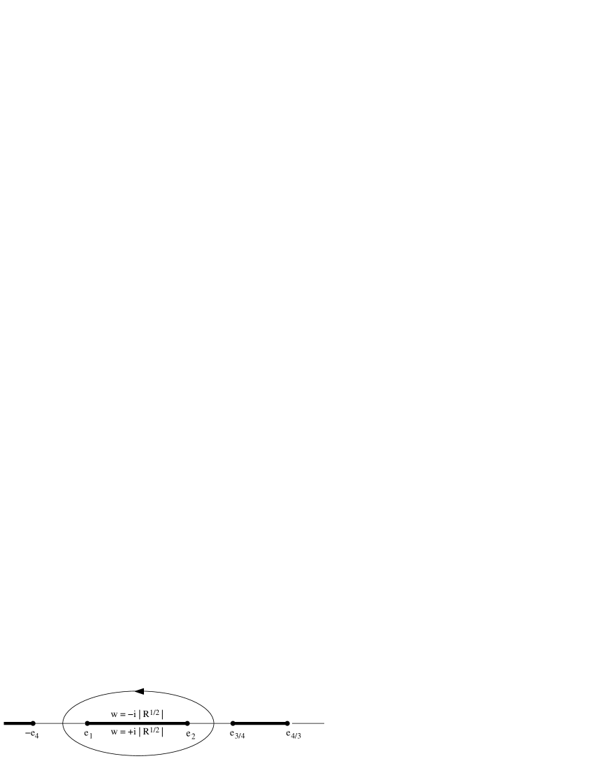
Figure 1: The top sheet of the hyperelliptic curve $C$.

Let $C$ be the hyperelliptic curve given by $w^{2}=R(u)$, where

$$R(u)=(u-e_{1})(u-e_{2})(u-e_{3})(u^{2}-e_{4}^{2}).$$

For future reference we remark that by comparison with equations (3.2) and (3.3),

$$R(u)=\left(u^{2}-1-\frac{A}{ps}\right)\left(\frac{1}{p}(1-u^{2})\left(h-\frac{1}{2C}\,n^{2}-pu\right)-\frac{1}{2Ap}(l-nu)^{2}\right).$$ (3.8)

The hyperelliptic curve $C$ is a two sheeted branched covering of the $u$-plane with the six branch points $e_{1}$, $e_{2}$, $e_{3}$, $e_{4}$, $-e_{4}$, and $\infty$. Figure 1 shows one sheet of $C$ with cuts along the real axis. This will be called the top sheet. Lift the path along which $u$ moves during the motion of the top to a path on the hyperelliptic curve which is homologous to the path drawn in the figure. Then

$$t=-i\sqrt{\frac{s}{2}}\int\left(u^{2}-{e_{4}}^{2}\right)\frac{du}{w}\,.$$ (3.9)

This is an Abelian integral of the second kind which has a simple pole at infinity: Introducing a holomorphic parameter $v^{2}=1/u$ around $\infty$, one obtains the asymptotic expansion $t=-i\sqrt{2s}v^{-1}+O(1)$ for $v\rightarrow 0$.

3.4 Hyperelliptic integrals for the Cayley-Klein parameters

In the following proposition, hyperelliptic integrals for the Cayley-Klein parameters are presented and their analytical properties discussed. These solutions are similar to the corresponding results for the Lagrange top. In the latter case, one obtains elliptic integrals and not hyperelliptic ones as here, but they have the same kind of singularities at corresponding places. Also, the reduction to the case $A=C$ of spherical tops works for the Lagrange top as well. According to F. Klein [7, p. 234], the reduction of Lagrange’s top to the spherical case was first noticed by Darboux.

Proposition 3.

Suppose first that $A=C$. Then the solution of the system is given by the hyperelliptic integrals

$$\begin{split}\log\alpha&=\int\frac{1}{2(u+1)}\left(w+\frac{u^{2}-{e_{4}}^{2}}{1-{e_{4}}^{2}}w_{-1}\right)\frac{du}{w}\\ \log\beta&=\int\frac{1}{2(u-1)}\left(w-\frac{u^{2}-{e_{4}}^{2}}{1-{e_{4}}^{2}}w_{+1}\right)\frac{du}{w}\\ \log\gamma&=\int\frac{1}{2(u-1)}\left(w+\frac{u^{2}-{e_{4}}^{2}}{1-{e_{4}}^{2}}w_{+1}\right)\frac{du}{w}\\ \log\delta&=\int\frac{1}{2(u+1)}\left(w-\frac{u^{2}-{e_{4}}^{2}}{1-{e_{4}}^{2}}w_{-1}\right)\frac{du}{w}\,.\end{split}$$ (3.10)

The constants $w_{\pm 1}$ denote one of the two values of $w$ on $C$ over $u=\pm 1$, i.e.

$$w_{+1}=\pm\sqrt{R(1)}\quad\text{and}\quad w_{-1}=\pm\sqrt{R(-1)}\,.$$

(There are four possible ways to choose, in accordance with the indeterminacy of $l$ and $n$ in terms of $e_{1},e_{2},e_{3}$; see Section 3.2).

They are Abelian integrals of the third kind, the differentials under the integral sign having two simple poles each, with residues $\pm 1$ at the places shown in Table 1, and no other singularities.

Table 1: The poles of the logarithmic differentials.

Differential	pole with res. 1 at	pole with res. -1 at
$d\alpha/\alpha$	$(u,w)=(-1,w_{-1})$	$\infty$
$d\beta/\beta$	$(u,w)=(+1,-w_{+1})$	$\infty$
$d\gamma/\gamma$	$(u,w)=(+1,w_{+1})$	$\infty$
$d\delta/\delta$	$(u,w)=(-1,-w_{-1})$	$\infty$

If $A\neq C$, the solution is

$$\Phi\cdot\begin{pmatrix}\exp(\frac{i}{2}\tau t)&0\\ 0&\exp(-\frac{i}{2}\tau t)\end{pmatrix},$$ (3.11)

where

$$\tau=\left(\frac{1}{C}-\frac{1}{A}\right)n.$$

I.e., the solution differs from the solution for the spherical top only by a rotation with constant speed around the top’s axis.

Proof.

First, the expressions for the logarithmic differentials of $\alpha,\beta,\gamma,\delta$ are derived in the general case. The reduction to the case of spherical tops is then immediate. Finally, the analytic properties of the differentials are examined.

Observe that

$$\begin{split}1&=\alpha\delta-\beta\gamma\\ u&=\alpha\delta+\beta\gamma.\end{split}$$ (3.12)

This implies

$$u+1=2\alpha\delta\text{\quad and\quad}u-1=2\beta\gamma,$$ (3.13)

such that

$$\begin{split}du&=2(\delta\,d\alpha+\alpha\,d\delta)\\ du&=2(\gamma\,d\beta+\beta\,d\gamma).\end{split}$$ (3.14)

By equations (2.2) and (2.3), the components of the angular velocity vector in the direction of the vertical axis and the top’s symmetry axis are given by

$$i\omega_{3} =2(\alpha^{\prime}\delta-\beta^{\prime}\gamma)=2(-\alpha\delta^{\prime}+\beta\gamma^{\prime}),$$

$$i\Omega_{3} =2(\delta\alpha^{\prime}-\beta\gamma^{\prime})=2(-\alpha\delta^{\prime}+\beta^{\prime}\gamma).$$

This implies

$$i(\Omega_{3}+\omega_{3})dt =2(\delta\,d\alpha-\alpha\,d\delta),$$

$$i(\Omega_{3}-\omega_{3})dt =2(\gamma\,d\beta-\beta\,d\gamma).$$

With equations (3.13) and (3.14) one obtains

$$\begin{split}du+i(\Omega_{3}+\omega_{3})dt&=4\,\delta\,d\alpha=2(u+1)\frac{d\alpha}{\alpha}\\ du+i(\Omega_{3}-\omega_{3})dt&=4\,\gamma\,d\beta=2(u-1)\frac{d\beta}{\beta}\\ du-i(\Omega_{3}-\omega_{3})dt&=4\,\beta\,d\gamma=2(u-1)\frac{d\gamma}{\gamma}\\ du-i(\Omega_{3}+\omega_{3})dt&=4\,\alpha\,d\delta=2(u+1)\frac{d\delta}{\delta}.\end{split}$$ (3.15)

Now it follows from $n=C\Omega_{3}$ and $l=A\omega_{3}+(C-A)\Omega_{3}u$ that

$$\Omega_{3}+\omega_{3} =\frac{1}{A}(l+n)+(u+1)\left(\frac{1}{C}-\frac{1}{A}\right)n,$$ (3.16)

$$\Omega_{3}-\omega_{3} =-\frac{1}{A}(l-n)-(u-1)\left(\frac{1}{C}-\frac{1}{A}\right)n.$$ (3.17)

Note that from equation (3.8),

$$R(\pm 1)=\frac{1}{2p^{2}s}(l\mp n)^{2}.$$

Hence the signs of $w_{\pm 1}$ can be chosen such that

$$w_{\pm 1}=\sqrt{\frac{s}{2}}\,\frac{1}{ps}\,(l\mp n),$$

or, from equation (3.5),

$$w_{\pm 1}=\sqrt{\frac{s}{2}}\,(1-{e_{4}}^{2})\,\frac{1}{A}(l\mp n).$$

Together with equation (3.16) and the equation for $dt$ obtained from (3.9), this yields

$$i(\Omega_{3}+\omega_{3})dt =\frac{u-{e_{4}}^{2}}{1-{e_{4}}^{2}}\,w_{-1}\,\frac{du}{w}+i(u+1)\left(\frac{1}{C}-\frac{1}{A}\right)n\,dt$$

$$-i(\Omega_{3}-\omega_{3})dt =\frac{u-{e_{4}}^{2}}{1-{e_{4}}^{2}}\,w_{+1}\,\frac{du}{w}+i(u-1)\left(\frac{1}{C}-\frac{1}{A}\right)n\,dt.$$

Substituting these expressions into (3.15), one obtains

$$\frac{d\alpha}{\alpha} =\frac{1}{2(u+1)}\left(w+\frac{u^{2}-{e_{4}}^{2}}{1-{e_{4}}^{2}}w_{-1}\right)\frac{du}{w}+\frac{i}{2}\left(\frac{1}{C}-\frac{1}{A}\right)n\,dt$$

$$\frac{d\beta}{\beta} =\frac{1}{2(u-1)}\left(w-\frac{u^{2}-{e_{4}}^{2}}{1-{e_{4}}^{2}}w_{+1}\right)\frac{du}{w}-\frac{i}{2}\left(\frac{1}{C}-\frac{1}{A}\right)n\,dt$$

$$\frac{d\gamma}{\gamma} =\frac{1}{2(u-1)}\left(w+\frac{u^{2}-{e_{4}}^{2}}{1-{e_{4}}^{2}}w_{+1}\right)\frac{du}{w}+\frac{i}{2}\left(\frac{1}{C}-\frac{1}{A}\right)n\,dt$$

$$\frac{d\delta}{\delta} =\frac{1}{2(u+1)}\left(w-\frac{u^{2}-{e_{4}}^{2}}{1-{e_{4}}^{2}}w_{-1}\right)\frac{du}{w}-\frac{i}{2}\left(\frac{1}{C}-\frac{1}{A}\right)n\,dt.$$

This implies equations (3.10) and the reduction to the spherical case.

Now assume that $A=C$. The assertions regarding the poles of the logarithmic differentials away from $\infty$ follow straightforwardly. Regarding the asymptotics at $\infty$, note that near $\infty$ the logarithmic differentials are

$$\frac{du}{2(u\pm 1)}+\text{\it a holomorphic part}.$$

Introduce the parameter $\xi^{2}=1/(u\pm 1)$. It is well defined (up to sign) and holomorphic around $\infty$. One finds that the singular part of the logarithmic differentials is $d\xi/\xi$. ∎

4 The trajectory of the tip of the top

In this section we examine the curve that the tip of the top describes in the horizontal plane. This aspect of the top’s motion is particularly easy to observe experimentally. For example, in toy shops one can buy tops that have a pencil lead for a tip or a felt tip pen. Lord Kelvin did experiments with such pencil tipped tops, while F. Klein used cogwheels from a clockwork which he spun on a sooty glass plate. See [7, pp. 619ff] for pictures and a discussion of the significant influence of friction and other concomitants neglected in the mathematical model.

4.1 Geometrical considerations

Since $r$ is the unit vector in the direction of the top’s axis, pointing away from the top’s tip if attached to the center of gravity, the curve traced by the tip of the top on the supporting plane is the orthogonal projection of $-sr$ onto that plane. The following proposition gives a formula for this curve in terms of the Cayley-Klein parameters.

Proposition 4.

Identify the supporting plane with the complex number plane. Then the curve traced by the tip of the top is

$$c=2s\alpha\beta.$$

Proof.

First, project the vector $-r$ stereographically from the north pole of the unit sphere into the complex plane. The result is the image of $0$ under the Möbius transformation (2.5), i.e. $z=\beta/\delta$. Since $\bar{z}=-\gamma/\alpha$, the fromula for $c$ follows from equations (2.4):

$$c=s(\xi+i\eta)=s\,\frac{2z}{|z|^{2}+1}\,.$$

This proves the proposition. ∎

For the qualitative considerations below, it is useful to represent the curve $c$ in polar coordinates: $c=\rho e^{i\phi}$. Clearly, $\rho=s\sqrt{1-u^{2}}$. The angle $\phi$ is not uniquely defined if $\rho$ vanishes, i.e. if $u=\pm 1$. Otherwise, the following proposition gives a formula for $d\phi$.

Proposition 5.

If $-1<u<1$, then

$$i\,d\phi=\frac{1}{2}\,\frac{u^{2}-{e_{4}}^{2}}{1-{e_{4}}^{2}}\left(\frac{w_{-1}}{u+1}-\frac{w_{+1}}{u-1}\right)\frac{du}{w}\,.$$ (4.1)

Proof.

The angle $\phi$ is the argument of the curve $z=2s\alpha\beta$. It follows that $d\phi$ is the imaginary part of the logarithmic differential $dc/c=d\alpha/\alpha+d\beta/\beta$. Formula (4.1) then follows from equations (3.10). ∎

4.2 Loop, cusp, or wobbly arc?

Figure 2: The curve traced by the tip of the top. Here, $w_{-1}$ and $w_{+1}$ have the same sign, $s=1,\ e_{1}=0.7,\ e_{2}=0.9,\ {e_{4}}^{2}=2$ and $e_{3}=1,\ 2,\ 100$ (left to right).

Figure 3: The curve traced by the tip of the top. Here, $w_{-1}$ and $w_{+1}$ have different signs, $s=1,\ e_{1}=0.7,\ e_{2}=0.9,\ {e_{4}}^{2}=2$ and $e_{3}=1,\ 1.1,\ 1.3,\ 1.85,\ 2.5,\ 3$ (top left to bottom right).

Figures 2 and 3 show different trajectories of the top’s tip. Three qualitatively different cases are clearly discernible. In Figure 2 and the top row of Figure 3, the curve is a smooth line circling the origin. The first picture on the bottom row of Figure 3 shows a cusp, and the following two show loops. The next proposition gives a condition in terms of $e_{1}$, $e_{2}$ and $e_{3}$ for the three cases to occur.

Proposition 6.

Assume that $-1<e_{1}$ and $e_{2}<1$. If $w_{+1}$ and $w_{-1}$ have the same sign, then the trajectory of the top’s tip has neither loops nor cusps. If $w_{+1}$ and $w_{-1}$ have different signs, then the curve has loops if and only if

$${\frac{1-e_{1}e_{2}}{e_{2}-e_{1}}}<e_{3}.$$

There are cusps if both sides are equal.

Proof.

Loops occur, if $d\phi/du$ changes sign as $u$ moves from $e_{1}$ to $e_{2}$. It follows from equation (4.1) that this happens if $w_{-1}/(u+1)-w_{+1}/(u-1)=0$ has a solution for $u$ in the interval $(e_{1},e_{2})$. That equation is equivalent to

$$\frac{u+1}{u-1}=\frac{w_{-1}}{w_{+1}}\,.$$ (4.2)

Since the left hand side of this equation is smaller than zero for $u\in(-1,1)$, this equation cannot be fulfilled if $w_{+1}$ and $w_{-1}$ have the same sign. This proves the first part of the proposition.

Now assume that $w_{+1}$ and $w_{-1}$ have different signs. Then

$$\frac{w_{-1}}{w_{+1}}=-\sqrt{\frac{(-1-e_{1})(-1-e_{2})(-1-e_{3})}{(1-e_{1})(1-e_{2})(1-e_{3})}}.$$

In the interval $[e_{1},e_{2}]$, the function $u\mapsto(u+1)/(u-1)$ is continuously decreasing from $(e_{1}+1)/(e_{1}-1)$ to $(e_{2}+1)/(e_{2}-1)$. Hence, equation (4.2) leads to a $u\in(e_{1},e_{2})$ if

$$\frac{e_{2}+1}{e_{2}-1}<-\sqrt{\frac{(-1-e_{1})(-1-e_{2})(-1-e_{3})}{(1-e_{1})(1-e_{2})(1-e_{3})}}<\frac{e_{1}+1}{e_{1}-1}\,.$$

This is equivalent to

$$-\frac{1-e_{3}}{1+e_{3}}<\frac{1+e_{1}}{1-e_{1}}\,\frac{1-e_{2}}{1+e_{2}}<-\frac{1+e_{3}}{1-e_{3}}.$$

The inequality on the right is always fulfilled, because the right hand side is greater than one and the left hand side smaller. The inequality on the left is equivalent to $(1-e_{1}e_{2})/(e_{2}-e_{1})<e_{3}$. This proves the condition for loops. If $(1-e_{1}e_{2})/(e_{2}-e_{1})=e_{3}$, then the zero of $d\phi/du$ occurs at $u=e_{2}$, hence there are cusps. ∎

5 The degenerate cases

If two zeroes of the polynomial $R(u)$ coincide, the hyperelliptic integrals of the Sections 3.3 and 3.4 degenerate to elliptic ones. In those cases, it is possible to solve the system in terms of elliptic functions. This will be done in the following sections. Since $-1\leq e_{1}\leq e_{2}\leq 1\leq e_{3}$ and $e_{4}>1$, only the following cases have to be considered: $e_{1}=e_{2}$, $e_{2}=e_{3}$ and $e_{3}=e_{4}$. Furthermore, the limit case $e_{4}=-e_{4}=\infty$ is examined, because it is of special interest: In this case the toy top becomes the Lagrange top.

5.1 The case $e_{3}=e_{4}$

Suppose that $e_{3}=e_{4}$. Then the hyperelliptic curve $C$ degenerates to the elliptic curve $C_{e_{3}=e_{4}}$, given by $w^{2}=R(u)$, where

$$R(u)=4(u-e_{1})(u-e_{2})(u+e_{3})\,.$$

The leading coefficient of $R$ is chosen to be 4 in accordance with the Weierstrass normalization of elliptic curves. This will simplify the integration of the elliptic integrals in terms of Weierstass elliptic functions $\wp,\zeta$ and $\sigma$. The branchpoints are $e_{1},e_{2},-e_{3}$, and $\infty$.

The $t$-integral and the integrals (3.10) become

$$t=-i\sqrt{2s}\int(u+e_{3})\frac{du}{w}\,,$$ (5.1)

and

$$\begin{split}\log\alpha&=\int\frac{1}{2(u+1)}\left(w+\frac{u+e_{3}}{-1+e_{3}}\,w_{-1}\right)\frac{du}{w}\\ \log\beta&=\int\frac{1}{2(u-1)}\left(w-\frac{u+e_{3}}{1+e_{3}}\,w_{+1}\right)\frac{du}{w}\\ \log\gamma&=\int\frac{1}{2(u-1)}\left(w+\frac{u+e_{3}}{1+e_{3}}\,w_{+1}\right)\frac{du}{w}\\ \log\delta&=\int\frac{1}{2(u+1)}\left(w-\frac{u+e_{3}}{-1+e_{3}}\,w_{-1}\right)\frac{du}{w}\,.\end{split}$$ (5.2)

As before, $w_{\pm 1}$ denotes one of the two values of $w$ on the curve $C_{e_{3}=e_{4}}$ over $u=\pm 1$, i.e

$$w_{+1}=\pm\sqrt{R(1)}\quad\text{and}\quad w_{-1}=\pm\sqrt{R(-1)}.$$

5.1.1 Uniformization of the elliptic curve

The system will be solved by using an Abelian integral of the first kind to uniformize the the elliptic curve $C_{e_{3}=e_{4}}$ and then expressing $t$ and $\alpha,\beta,\gamma,\delta$ as functions of the uniformizing variable.

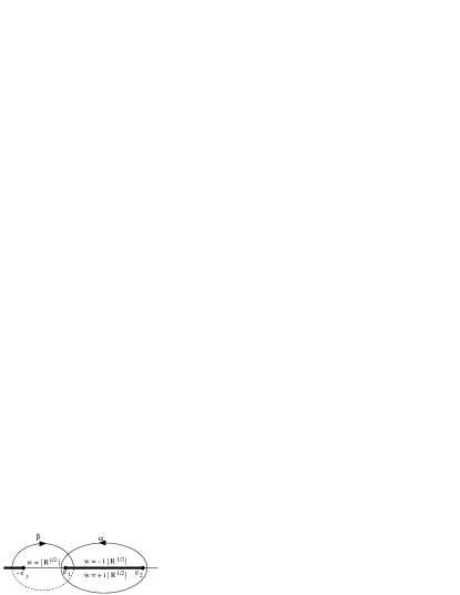
Figure 4: Left: The top sheet of the elliptic curve $C_{e_{3}=e_{4}}$. Right: A fundamental domain in the $x$-plane.

The left part of Figure 4 shows the top sheet of the curve $C_{e_{3}=e_{4}}$ with cuts and a normal cycle basis $\alpha,\beta.$ Let $\omega_{1}$ and $\omega_{2}$ be the corresponding half periods:

$$2\omega_{1}=\int_{\alpha}\frac{du}{w},\quad 2\omega_{2}=\int_{\beta}\frac{du}{w}\,.$$

Note that $\omega_{1}$ lies on the negative imaginary axis and that $\omega_{2}$ is positive. Let the uniformizing variable be given by

$$x=\int_{u=e_{2}}^{u=u(x)}\frac{du}{w}.$$ (5.3)

One obtains $u$ and $w$ as doubly periodic functions of $x$ with periods $2\omega_{1}$ and $2\omega_{2}$, namely

$$u(x)=\wp(x-\omega_{2})+\frac{1}{3}(e_{1}+e_{2}-e_{3})$$ (5.4)

and

$$w(x)=\wp^{\prime}(x-\omega_{2}).$$ (5.5)

The additive constant $(e_{1}+e_{2}-e_{3})/3$ in (5.4) comes from the fact that the branchpoints are not centered around zero as required by the Weierstrass normalization, and the $\wp$-function is shifted by $\omega_{1}$ because the integral in (5.3) does not start in $\infty$ but $e_{2}$.

The right part of Figure 4 shows a fundamental rectangle in the $x$-plane. The points $x=\pm a$ and $x=\pm b$ will be of importance in Section 5.1.3 and are defined as follows: The point $a$ in the $x$-plane is supposed to correspond to the point $(u,w)=(-1,w_{-1})$ on $C_{e_{3}=e_{4}}$, and $b$ is supposed to correspond to $(u,w)=(+1,w_{+1})$. For example, let

$$a=\pm\left(\omega_{1}+\int_{-1}^{e_{1}}\sqrt{R(u)}\,du\right)$$

and

$$b=\pm\int_{e_{2}}^{1}\sqrt{R(u)}\,du,$$

where the signs are chosen according to whether the points $(u,w_{\pm 1})$ lie in the bottom or top sheet. (The figure shows the case where both $x=a$ and $x=b$ correspond to points in the bottom sheet. Otherwise exchange $+a$ with $-a$, or $+b$ with $-b$, respectively.)

Regarding the toy top we adopt the convention that during its motion, the corresponding point on $C_{e_{3}=e_{4}}$ moves on a path homotopic to the cycle $\alpha$. (This choice determines the sign on the right hand side of equation (5.1)). The corresponding point in the $x$-plane then moves on the imaginary axis in the negative direction.

5.1.2 Solution for time as function of the uniformizing variable

We will now pull back the $t$-integral (5.1) to the $x$ plane and solve it. The following proposition gives the resulting formula for $t$ as function of $x$. The initial condition which is chosen means that $u=e_{2}$ at $t=0$, i.e. the axis of the top is initially in its most upright position.

Proposition 7.

Assume that $t=0$ for $x=0$. Then equation (5.1) implies

$$t=i\sqrt{2s}\big{(}\zeta(x-\omega_{2})+\zeta(\omega_{2})-\frac{1}{3}(e_{1}+e_{2}+2e_{3})\,x\big{)}.$$

Proof.

Equations (5.4) and (5.5) imply that the pullback of the holomorphic differential $du/w$ to the $x$-plane is $dx$. The $t$-integral therefore becomes

$$t=-i\sqrt{2s}\int\big{(}\wp(x-\omega_{2})+\frac{1}{3}(e_{1}+e_{2}+2e_{3})\big{)}dx.$$

Since $\zeta^{\prime}=-\wp$, this implies

$$t=i\sqrt{2s}\big{(}\zeta(x-\omega_{2})-\frac{1}{3}(e_{1}+e_{2}+2e_{3})x+\mbox{\em const.}\big{)}.$$

The constant has to be $\zeta(\omega_{2})$ for $t$ to vanish at $x=0$. ∎

5.1.3 Solution for the Cayley-Klein parameters as functions of the uniformizing variable

The following proposition gives formulas for $\alpha,\beta,\gamma,\delta$ as functions of $x$. But first, a few words have to be said about the initial conditions $\alpha_{0},\beta_{0},\gamma_{0},\delta_{0}$ for $t=x=0$.

It is no essential restriction to assume that $\alpha_{0}$ is real and nonnegative and therefore equals $\delta_{0}$, and that $\gamma_{0}$ is purely imaginary with nonnegative imaginary part, such that $\beta_{0}=\gamma_{0}$. For one may always achieve this by suitable rotations of the system about the $z$-Axis and the top’s symmetry axis.

Proposition 8.

Under the above initial conditions, one obtains

$$\begin{split}\alpha=k_{1}e^{l_{1}x}\frac{\sigma(x-a)}{\sigma(x-\omega_{2})},\\ \beta=k_{2}e^{l_{2}x}\frac{\sigma(x+b)}{\sigma(x+\omega_{2})},\\ \gamma=k_{3}e^{l_{3}x}\frac{\sigma(x-b)}{\sigma(x-\omega_{2})},\\ \delta=k_{4}e^{l_{4}x}\frac{\sigma(x+a)}{\sigma(x+\omega_{2})},\end{split}$$ (5.6)

where

$$\begin{split}k_{1}&=k_{4}=\sqrt{\frac{1+e_{2}}{2}}\;\frac{\sigma(\omega_{2})}{\sigma(a)},\\ k_{2}&=k_{3}=\,i\,\sqrt{\frac{1-e_{2}}{2}}\;\frac{\sigma(\omega_{2})}{\sigma(b)},\end{split}$$ (5.7)

and

$$\begin{split}l_{1}&=-l_{4}=\frac{w_{-1}}{2(-1+e_{3})}+\zeta(a-\omega_{2}),\\ l_{3}&=-l_{2}=\frac{w_{+1}}{2(1+e_{3})}+\zeta(b-\omega_{2}).\end{split}$$ (5.8)

Proof.

Consider the asymptotic behavior of the logarithmic differential of $\alpha$:

$$\frac{d\alpha}{\alpha}=\frac{1}{2(u+1)}\left(w+\frac{u+e_{3}}{-1+e_{3}}\,w_{-1}\right)\frac{du}{w}.$$

It has only two simple poles on $C_{e_{3}=e_{4}}$, one at $(u,w)=(-1,w_{-1})$ and the other at $\infty$. For $(u,w)\rightarrow(-1,w_{-1})$, the asymptotic expansion is

$$\frac{d\alpha}{\alpha}=\left(\frac{1}{u+1}+O(1)\right)du.$$

To calculate the asymptotic expansion around the branchpoint $\infty$, introduce the local parameter $\xi^{2}=1/u$. The result is

$$\frac{d\alpha}{\alpha}=\left(-\frac{1}{\xi}+O(1)\right)d\xi.$$

Since the residues of the logarithmic differential of $\alpha$ are $1$ and $-1$, respectively, $\alpha$ itself is not branched on $C_{e_{3}=e_{4}}$, but has a zero at $(u,w)=(-1,w_{-1})$ and a simple pole at $\infty$. It is a multiply valued function, because the additive periods of the logarithmic differential lead to multiplicative periods of $\alpha$. It follows that, in terms of the uniformizing variable $x$, $\alpha$ is of the form

$$\alpha=k_{1}e^{l_{1}x}\frac{\sigma(x-a)}{\sigma(x-\omega_{2})}.$$

Similarly, one obtains the other equations (5.6).

The constants $k_{1},\ldots,k_{4}$ and $l_{1},\ldots,l_{4}$ are determined by the initial conditions. Note first that $\alpha_{0}=\delta_{0}$ implies $k_{1}=k_{4}$ and $\beta_{0}=\gamma_{0}$ implies $k_{2}=k_{3}$. Just substitute $x=0$ into equations (5.6) and observe that $\sigma$ is an odd function.

Further, since $u=e_{2}$ for $x=0$, it follows from equations (3.13) that

$$e_{2}+1=2\alpha_{0}\delta_{0}=2{k_{1}}^{2}\frac{\sigma^{2}(a)}{\sigma^{2}(\omega_{2})}$$

and

$$e_{2}-1=2\beta_{0}\gamma_{0}=2{k_{2}}^{2}\frac{\sigma^{2}(b)}{\sigma^{2}(\omega_{2})}.$$

From this one obtains equations (5.7). The signs of $k_{1}$ and $k_{2}$ are determined so that $\alpha_{0}$ is positive and $\gamma_{0}$ has a positive imaginary part.

Concerning the constants $l_{1},\ldots,l_{4}$, note first that

$$\frac{u+1}{2}=\alpha\delta=k_{1}k_{4}e^{(l_{1}+l_{4})x}\frac{\sigma(x-a)\sigma(x+a)}{\sigma(x-\omega_{2})\sigma(x+\omega_{2})}$$

is a doubly periodic function of $x$. This implies $l_{4}=-l_{1}$ since the quotient of $\sigma$-functions is already doubly periodic. Equally, considering $\beta\gamma=(u-1)/2$ yields $l_{2}=-l_{3}$.

From the logarithmic derivative of $\alpha$ with respect to $x$

$$\frac{d\log\alpha}{dx}=l_{1}+\frac{\sigma^{\prime}(x-a)}{\sigma(x-a)}-\frac{\sigma^{\prime}(x-\omega_{2})}{\sigma(x-\omega_{2})}$$

one obtains

$$l_{1}=\frac{d\log\alpha}{dx}-\zeta(x-a)+\zeta(x-\omega_{2}),$$

since $\sigma^{\prime}/\sigma=\zeta$. The first of equations then (5.8) follows from

$$\lim_{x\rightarrow a}\left(\frac{d\log\alpha}{dx}-\zeta(x-a)\right)=\frac{w_{-1}}{2(-1+e_{3})}\,.$$

Since $\zeta(x-a)=1/(x-a)+O(x-a)$ as $x\rightarrow a$, one has to show that

$$\frac{d\log\alpha}{dx}=\frac{1}{x-a}+\frac{w_{-1}}{2(-1+e_{3})}+O(x-a).$$ (5.9)

From the first equation (5.2) and $dx=du/w$ one obtains

$$\frac{d\log\alpha}{dx}=\frac{1}{2(u+1)}\left(w+\frac{u+e_{3}}{-1+e_{3}}\,w_{-1}\right).$$

Since $w=du/dx$, this yields the expansion

$$\frac{d\log\alpha}{dx} =\frac{1}{2(u+1)}\left(\left.\frac{du}{dx}\right|_{\makebox[0.0pt][l]{$\scriptstyle x=a$}}+(x-a)\left.\frac{d^{2}u}{dx^{2}}\right|_{\makebox[0.0pt][l]{$\scriptstyle x=a$}}+O(x-a)^{2}+\left(1+\frac{u+1}{-1+e_{3}}\right)w_{-1}\right)$$

$$=\frac{1}{u+1}\left.\frac{du}{dx}\right|_{x=a}+\frac{1}{2}\left.\frac{\,\frac{d^{2}u}{dx^{2}}\,}{\frac{du}{dx}}\right|_{x=a}+\frac{w_{-1}}{2(-1+e_{3})}+O(x-a)\,.$$ (5.10)

The last equality uses

$$\frac{x-a}{u+1}=\frac{1}{\left.\frac{du}{dx}\right|_{\makebox[0.0pt][l]{$\scriptstyle x=a$}}}+O(x-a).$$ (5.11)

The asymptotical expansion (5.9) follows from (5.1.3) and

$$\frac{1}{x-a}=\frac{1}{u+1}\left.\frac{du}{dx}\right|_{x=a}+\frac{1}{2}\left.\frac{\,\frac{d^{2}u}{dx^{2}}\,}{\frac{du}{dx}}\right|_{x=a}+O(x-a).$$

To see this last equation, just take the Taylor expansion

$$u+1=\left.\frac{du}{dx}\right|_{x=a}(x-a)+\frac{1}{2}\left.\frac{d^{2}u}{dx^{2}}\right|_{x=a}(x-a)^{2}+O(x-a)^{3},$$

divide by $(x-a)$ and $(u+1)$, and use (5.11) again. The equation for $l_{3}$ is derived analogously. ∎

5.2 The case of regular precession

If a spinning top moves in such a way that the angle between the top’s axis and the vertical is constant, its motion is called regular precession. It then follows from the symmetries of the system that the top spins around its axis with constant speed, while the axis precedes uniformly around the vertical axis. Notably, the solutions for $t$ and the Cayley-Klein parameters in terms of hyperelliptic integrals fail in the case of regular precession because the path of integration degenerates to a point. One would have to look at the system before it is completely reduced to analyze this case. It turns out that regular precession occurs if $R(u)$ has a double zero at the constant value for $u$. There are two qualitatively different ways this can happen. If $e_{1}=e_{2}$, small perturbations of the system will lead to small nutation. The regular precession is stable. But if $e_{2}=e_{3}=1$, small perturbations will lead to nutation between $u=e_{1}$ and $u=e_{2}$. The regular precession is unstable. See [7, pp. 278ff] for an analogous discussion of the stability of regular precession in the case of Lagrange’s top.

5.3 The aperiodic case: $e_{2}=e_{3}=1$

If $e_{2}=e_{3}$, there are two possible types of motion. Either $u$ is constantly 1. This is the unstable case of regular precession mentioned above. Or $u$ moves from 1 to $e_{1}$ and back. This case will be considered in this section. We proceed similarly as in Section 5.1.

The hyperelliptic curve $C$ degenerates to the elliptic curve $C_{\text{aper}}$ given by $w^{2}=R(u)$ with

$$R(u)=4(u-e_{1})(u^{2}-{e_{4}}^{2}).$$

Branchpoints are $e_{1}$, $\pm e_{4}$ and $\infty$. The $t$-integral becomes

$$t=i\,\sqrt{2s}\int\frac{(u^{2}-{e_{4}}^{2})}{u-1}\,\frac{du}{w}.$$ (5.12)

It is singular at $u=1$. That is why this is the aperiodic case. The integrals (3.10) become

$$\begin{split}\log\alpha&=\int\frac{1}{2(u+1)}\left(w-\frac{2}{u-1}\,\frac{u^{2}-{e_{4}}^{2}}{1-{e_{4}}^{2}}w_{-1}\right)\frac{du}{w}\\ \log\beta&=\int\frac{du}{2(u-1)}\\ \log\gamma&=\int\frac{du}{2(u-1)}\\ \log\delta&=\int\frac{1}{2(u+1)}\left(w+\frac{2}{u-1}\,\frac{u^{2}-{e_{4}}^{2}}{1-{e_{4}}^{2}}w_{-1}\right)\frac{du}{w}\;.\end{split}$$ (5.13)

5.3.1 Uniformization of the elliptic curve

Figure 5 shows one sheet of $C_{\text{aper}}$, which will be called the top sheet. Proceed as in Section 5.1.1, but let the curves $c$ start in $(u,w)=(e_{1},0)$. For a normalized cycle basis, take a path $\alpha$ in the top sheet which encircles $e_{1}$ and $e_{4}$ in the counterclockwise direction, and choose $\beta$ accordingly. Let $\omega_{1}$ and $\omega_{2}$ be the corresponding half periods and let $\omega_{3}=\omega_{1}+\omega_{2}$. One obtains the uniformization

$$u=\wp(x-\omega_{3})+\frac{e_{1}}{3}$$

and $w=\wp^{\prime}(x-\omega_{3})$.

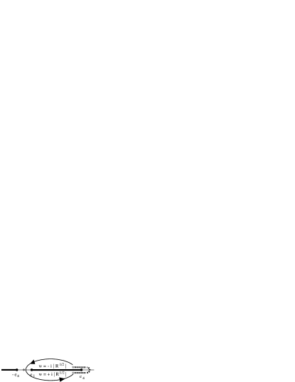
Figure 5: Left: The top sheet of the elliptic curve $C_{\text{aper}}$. Right: A fundamental domain in the $x$-plane.

The right part of Figure 5 shows a fundamental domain in the $x$-plane. Again, the points above $u=\pm 1$ will be important. In the figure, they are marked by asterisks. Let $a$ and $b$ be points in the $x$-plane corresponding to $(u,w)=(-1,w_{-1})$ and $(u,w)=(+1,w_{+1})$, for example,

$$a=\pm\int_{-1}^{e_{1}}\sqrt{R(u)}\,du\quad\text{and}\quad b=\pm i\int_{e_{1}}^{1}\sqrt{-R(u)}\,du.$$

(In the figure they are drawn for the case in which $(-1,w_{-1})$ lies in the top sheet and $w_{+1}$ has positive imaginary part.)

Let the path of integration corresponding to the motion of the top be homotopic the the path with arrows drawn in the figure.

5.3.2 Solution for time as function of the uniformizing variable

The integrand of the $t$-integral has simple poles over $u=1$ which leads to logarithmic type singularities for $t$. The Riemann surface of the function $t$ will therefore be an infinitely sheeted cover of $C_{\text{aper}}$ with the two branchpoints $(u,w)=(1,\pm w_{+1})$. Place a cut on $C_{\text{aper}}$ along the dotted line in Figure 5 and cut the $x$-plane along corresponding lines. Then our path of integration on $C_{\text{aper}}$ does not cross the cut, so that we can consider only one branch of the function $t$ on the cut elliptic curve, or the cut $x$-plane, respectively.

Proposition 9.

Suppose that $t=0$ at $x=0$. Then

$$\frac{t}{i\sqrt{2s}}= -\zeta(x-\omega_{3})-\zeta(\omega_{3})+\left(1+\frac{e_{1}}{3}\right)x$$

$$+\frac{1-{e_{4}}^{2}}{w_{+1}}\left(\log\left(-\frac{\sigma(x-b)}{\sigma(x+b)}\right)+2\big{(}\zeta(\omega_{3})-\zeta(b-\omega_{3})\big{)}x\right),$$

where that branch of the function

$$\log\left(-\frac{\sigma(x-b)}{\sigma(x+b)}\right)$$

is chosen that is zero for $x=0$.

Proof.

Put equation (5.12) in the form

$$t=i\sqrt{2s}\int\left(u+1+\frac{1-{e_{4}}^{2}}{u-1}\right)\frac{du}{w}$$ (5.14)

and consider separately the integrals

$$I_{1}=\int\frac{1}{u-1}\;\frac{du}{w}$$

and

$$I_{2}=\int(u+1)\,\frac{du}{w}\,.$$

Substituting the uniformizing variable in the first integral, we get

$$I_{1} =\int\frac{dx}{\wp(x-\omega_{3})-\wp(b-\omega_{3})}$$

$$=\frac{1}{\wp^{\prime}(b-\omega_{3})}\int\frac{\wp^{\prime}(b-\omega_{3})\,dx}{\wp(x-\omega_{3})-\wp(b-\omega_{3})}.$$

Using the formula

$$\frac{\wp^{\prime}(\eta)}{\wp(\xi)-\wp(\eta)}=\zeta(\xi-\eta)-\zeta(\xi+\eta)+2\zeta(\eta),$$

one obtains

$$I_{1} =\frac{1}{\wp^{\prime}(b-\omega_{3})}\int\big{(}\zeta(x-b)-\zeta(x+b-2\omega_{3})+2\zeta(b-\omega_{3})\big{)}dx$$

$$=\frac{1}{\wp^{\prime}(b-\omega_{3})}\int\big{(}\zeta(x-b)-\zeta(x+b)+2\zeta(\omega_{3})+2\zeta(b-\omega_{3})\big{)}dx.$$

The last equality follows from $\zeta(\xi+2\omega_{k})=\zeta(\xi)+2\zeta(\omega_{k}).$ Now the last integral can easily be solved since $\zeta(\xi)={\sigma^{\prime}(\xi)}/{\sigma(\xi)}$. Note that

$$\wp^{\prime}(b-\omega_{3})=w_{+1}$$

to obtain

$$I_{1}=\frac{1}{w_{+1}}\left(\log\left(\frac{\sigma(x-b)}{\sigma(x+b)}\right)+2\big{(}\zeta(\omega_{3})+\zeta(b-\omega_{3})\big{)}x+\mbox{\em const.}\right).$$

Requiring that $I_{1}=0$ for $x=0$, one obtains

$$I_{1}=\frac{1}{w_{+1}}\left(\log\left(-\frac{\sigma(x-b)}{\sigma(x+b)}\right)+2\big{(}\zeta(\omega_{3})+\zeta(b-\omega_{3})\big{)}x\right),$$ (5.15)

where that branch of the logarithmic term is chosen that vanishes for $x=0$. The other integral is easier to deal with:

$$I_{2} =\int\big{(}\wp(x-\omega_{3})+1+e_{1}/3\big{)}$$

$$=-\zeta(x-\omega_{3})+(1+e_{1}/3)x+\mbox{\em const.},$$

since $\wp=-\zeta^{\prime}$. If the constant is chosen to make $I_{2}$ vanish for $x=0$, this becomes

$$I_{2}=-\zeta(x-\omega_{3})-\zeta(\omega_{3})+\left(1+\frac{e_{1}}{3}\right)x.$$ (5.16)

The formula for $t$ follows from equations (5.14), (5.15) and (5.16). ∎

5.3.3 Solution for the Cayley-Klein parameters

The functions $\alpha,\beta,\gamma,\delta$ are also branched at the points above $u=1$. So we apply the same cut as in the previous section and have to choose branches. As in Section 5.1 we will assume that the initial conditions $\alpha_{0}$ and $\delta_{0}$ are real (and therefore equal) and positive, and that $\beta_{0}$ and $\gamma_{0}$ are imaginary (and therefore equal) with positive imaginary part.

Proposition 10.

If the initial conditions are chosen as explained above, then

$$\begin{split}\alpha&=ke^{lx-i\pi p}\frac{\sigma(x-a)}{\sigma(x-\omega_{3})}\left(\frac{\sigma(x+b)}{\sigma(x-b)}\right)^{p}\\ \gamma&=\beta=i\sqrt{\frac{1-u}{2}}\\ \delta&=ke^{-lx+i\pi p}\frac{\sigma(x+a)}{\sigma(x+\omega_{3})}\left(\frac{\sigma(x-b)}{\sigma(x+b)}\right)^{p},\end{split}$$

where

$$p=-\frac{1}{2}\,\frac{w_{-1}}{w_{+1}},$$

$$k=\sqrt{\frac{1+e_{1}}{2}}\,\frac{\sigma(\omega_{3})}{\sigma(a)},$$

$$l=\frac{w_{-1}}{4}-\frac{w_{-1}}{1-{e_{4}}^{2}}+\zeta(a-\omega_{3})-p\big{(}\zeta(a+b)+\zeta(a-b)),$$

and those branches of the multiply valued functions $(\sigma(x+b)/\sigma(x-b))^{p}$ and
$(\sigma(x-b)/\sigma(x+b))^{p}$ are chosen which take the values $e^{i\pi p}$ and $e^{-i\pi p}$ at $x=0$.

Proof.

The formula for $\beta$ and $\gamma$ follows elementarily from the corresponding integrals (5.13) and the initial conditions. Now consider the logarithmic differential of $\alpha$ from equations (5.13):

$$\frac{d\alpha}{\alpha}=\left(\frac{1}{2(u+1)}-\frac{1}{(u-1)(u+1)}\,\frac{w_{-1}}{w}-\frac{1}{1-{e_{4}}^{2}}\,\frac{w_{-1}}{w}\right)du.$$

As one can read off from this expression, the differential has three simple poles away from infinity, one at $(u,w)=(-1,w_{-1})$ with residue $1$ and two more at $(u,w)=(+1,\pm w_{+1})$ with residues $\mp w_{-1}/2w_{+1}$. Furthermore, the term $du/2(u+1)$ contributes one more simple pole at infinity with residue $-1$.

Table 2: The simple poles of $d\alpha/\alpha$ and $d\delta/\delta$ with residues.

$d\alpha/\alpha$
$(u,w)=$	$(-1,w_{-1})$	$\quad\infty\quad$	$(+1,+w_{+1})$	$(+1,-w_{+1})$
Residue:	1	-1	$-w_{-1}/2w_{+1}$	$w_{-1}/2w_{+1}$
$d\delta/\delta$
$(u,w)=$	$(-1,-w_{-1})$	$\quad\infty\quad$	$(+1,+w_{+1})$	$(+1,-w_{+1})$
Residue:	1	-1	$w_{-1}/2w_{+1}$	$-w_{-1}/2w_{+1}$

The location of the poles with their residues is summarized in Table 2. It also lists the poles of the logarithmic differential of $\beta$, which are obtained similarly. Now the poles with residue $\pm 1$ lead to zeroes and poles of $\alpha$ and $\delta$, while the other poles give rise to branchpoints. It follows that, as functions of $x$, $\alpha$ and $\delta$ are of the form

$$\begin{split}\alpha&=k_{1}e^{l_{1}x}\frac{\sigma(x-a)}{\sigma(x-\omega_{3})}\left(\frac{\sigma(x+b)}{\sigma(x-b)}\right)^{p}\\ \beta&=k_{2}e^{l_{2}x}\frac{\sigma(x+a)}{\sigma(x+\omega_{3})}\left(\frac{\sigma(x-b)}{\sigma(x+b)}\right)^{p}.\end{split}$$ (5.17)

Choose the branches of these multiply valued functions as explained in the proposition. Then the values

$$k_{1} =\sqrt{\frac{1+e_{1}}{2}}\,\frac{\sigma(\omega_{3})}{\sigma(a)}\,e^{-i\pi p}$$

$$k_{2} =\sqrt{\frac{1+e_{1}}{2}}\,\frac{\sigma(\omega_{3})}{\sigma(a)}\,e^{+i\pi p}$$

follow from the initial condition $\alpha_{0}=\delta_{0}=\sqrt{(1+e_{1})/2}$.

Since $2\alpha\delta=u+1$ is a doubly periodic function of $x$, it follows that $l_{2}=-l_{1}$. It is left to show that $l_{1}=l$ as given in the proposition. Since from equation (5.17)

$$\frac{d\log\alpha}{dx}=l_{1}+\zeta(x-a)-\zeta(x-\omega_{3})+p\big{(}\zeta(x+b)-\zeta(x-b)\big{)},$$

this will be achieved if we can prove that for $x\rightarrow a$,

$$\frac{d\log\alpha}{dx}=\frac{1}{x-a}+\frac{w_{-1}}{4}-\frac{w_{-1}}{1-{e_{4}}^{2}}+O(x-1).$$

This follows by a calculation analogous to the one in Section 5.1. ∎

5.4 The Lagrange top as limit case: $e_{4}=-e_{4}=\infty$

Look at the $t$-integral as it is written in equation (3.7). If one simply lets $e_{4}$ tend to infinity, the integrand diverges. But note that from equation (3.5) one obtains

$$-\frac{s}{2}=\frac{A}{2p}\,\frac{1}{1-{e_{4}}^{2}},$$

so that equation (3.7) can be rewritten as

$$t=\sqrt{\frac{A}{2p}}\int\sqrt{\frac{u^{2}-{e_{4}}^{2}}{1-{e_{4}}^{2}}}\frac{du}{\sqrt{(u-e_{1})(u-e_{2})(u-e_{3})}}.$$

Now if one lets $e_{4}$ tend to infinity while keeping $A/p$ constant, this converges to the Abelian integral of the first kind

$$t=\sqrt{\frac{A}{2p}}\int\frac{du}{w}$$

on the elliptic curve $w^{2}=(u-e_{1})(u-e_{2})(u-e_{3})$.

The integrals (3.10) cause no problems. They become

$$\begin{split}\log\alpha&=\int\frac{w+w_{-1}}{2(u+1)}\,\frac{du}{w}\\ \log\beta&=\int\frac{w-w_{+1}}{2(u-1)}\,\frac{du}{w}\\ \log\gamma&=\int\frac{w+w_{+1}}{2(u-1)}\,\frac{du}{w}\\ \log\delta&=\int\frac{w-w_{-1}}{2(u+1)}\,\frac{du}{w}\,.\end{split}$$

This is exactly the solution F. Klein obtains for the Lagrange top [7, p. 238],[3, pp. 28f]. This is not surprising since this limiting case is obtained by letting $s$ tend to zero while keeping all other parameters constant. But in this case the Lagrangian (3.1) coincides with the one of Lagrange’s top.

References

- [1] Dubrovin B.A., Krichever I.M. and Novikov S.P., Integrable Systems I, in Dynamical Systems IV, Editors V.I. Arnol’d and S.P. Novikov, in Encyclopaedia of Mathematical Sciences, no. 4, Springer, Berlin, 1990, 173–280.
- [2] Olshanetsky M.A., Perelomov A.M., Reyman A.G. and Semenov-Tian-Shansky M.A., Integrable Systems II, in Dynamical Systems VII, Editors V.I. Arnol’d and S.P. Novikov, in Encyclopaedia of Mathematical Sciences, no. 16, Springer, Berlin, 1994, 83–259.
- [3] Klein F., The Mathematical Theory of the Top, in Congruence of Sets and other Monographs, Chelsea Publishing Company, New York, Lectures delivered in Princeton in 1896.
- [4] Poisson S.D., Lehrbuch der Mechanik, vol. 2, G. Reimer, Berlin, 1836, Transl. from 2nd ed.
- [5] Whittaker E.T., A Treatise on the Analytical Dynamics of Particles and Rigid Bodies, 4th ed., Cambridge University Press, Cambridge, 1988, First published 1904.
- [6] Klein F., Einleitung in die analytische Mechanik, Teubner, Stuttgart and Leipzig, 1991, Lectures, held in Göttingen 1886/87.
- [7] Klein F. and Sommerfeld A., Über die Theorie des Kreisels, B. G. Teubner, Stuttgart, 1965, Reprint of the 1897-1910 ed.
- [8] Bobenko A.I. and Suris Y.B., Discrete Time Lagrangian Mechanics on Lie groups, with an Application to the Lagrange Top, Communications in Mathematical Physics, 1999, V.204, 147–188.
- [9] Bobenko A.I. and Suris Y.B., Discrete Lagrangian Reduction, Discrete Euler-Poincaré Equations, and Semidirect Products, Letters in Mathematical Physics, 1999, V.49, 79–93.
- [10] Klein F., Vorlesungen über das Ikosaeder und die Auflösung der Gleichungen vom fünften Grade, Teubner, Leipzig, 1993, Reprint of the 1884 ed.