UNKNOTTING VIRTUAL KNOTS WITH GAUSS DIAGRAM FORBIDDEN MOVES

SAM NELSON
Department of Mathematics, Louisiana State University
Baton Rouge, LA 70803
nelson@math.lsu.edu

abstract

The forbidden moves can be combined with Gauss diagram Reidemeister moves to obtain move sequences with which we may change any Gauss diagram (and hence any virtual knot) into any other, including in particular the unknotted diagram.

In 1996 Kauffman [1] introduced the theory of virtual knots, extending the topological concept of β€œknots” to include general Gauss codes. In 1999 Goussarov, Polyak and Viro [2] described virtual knots in terms of Gauss diagrams, which provide a visual way to represent Gauss codes.
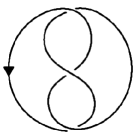
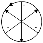
Consider a classical knot diagram $K\subset\mathbf{R}^{2}$ as an immersion $K:S^{1}\to\mathbf{R}^{2}$ of the circle in the plane with crossing information specified at each double point. A Gauss diagram for a classical knot diagram is an oriented circle considered as the preimage of the immersed circle with chords connecting the preimages of each double point. We specify crossing information on each chord by directing the chord toward the undercrossing point and decorating each with with signs specifying the local writhe number.

Refer to captionRefer to caption
Figure 1: A simple knot and its Gauss Diagram

A virtual knot is an equivalence class of Gauss diagrams under the relations in Figure 2, which are the classical Reidemeister moves written in terms of Gauss diagrams. Note that there are several variations of move III depending on the orientations of the strands; we only depict two.

Refer to captionβ€‹βŸ·I​Refer to captionRefer to captionβ€‹βŸ·I​Refer to captionRefer to captionFRACOP⟷IRefer to captionRefer to captionFRACOP⟷IRefer to caption\raisebox{-36.135pt}{\includegraphics[width=72.26999pt,height=72.26999pt]{i1.eps}}{\longleftrightarrow\atop\mathrm{I}}\raisebox{-36.135pt}{\includegraphics[width=72.26999pt,height=72.26999pt]{i2.eps}}\raisebox{-36.135pt}{\includegraphics[width=72.26999pt,height=72.26999pt]{i3.eps}}{\longleftrightarrow\atop\mathrm{I}}\raisebox{-36.135pt}{\includegraphics[width=72.26999pt,height=72.26999pt]{i4.eps}}
Refer to captionβ€‹βŸ·II​Refer to captionRefer to captionβ€‹βŸ·II​Refer to captionRefer to captionFRACOP⟷IIRefer to captionRefer to captionFRACOP⟷IIRefer to caption\raisebox{-36.135pt}{\includegraphics[width=72.26999pt,height=72.26999pt]{ii1.eps}}{\longleftrightarrow\atop\mathrm{II}}\raisebox{-36.135pt}{\includegraphics[width=72.26999pt,height=72.26999pt]{ii2.eps}}\raisebox{-36.135pt}{\includegraphics[width=72.26999pt,height=72.26999pt]{ii3.eps}}{\longleftrightarrow\atop\mathrm{II}}\raisebox{-36.135pt}{\includegraphics[width=72.26999pt,height=72.26999pt]{ii4.eps}}
Refer to captionβ€‹βŸ·III​Refer to captionRefer to captionβ€‹βŸ·III​Refer to captionRefer to captionFRACOP⟷IIIRefer to captionRefer to captionFRACOP⟷IIIRefer to caption\raisebox{-36.135pt}{\includegraphics[width=72.26999pt,height=72.26999pt]{iii1.eps}}{\longleftrightarrow\atop\mathrm{III}}\raisebox{-36.135pt}{\includegraphics[width=72.26999pt,height=72.26999pt]{iii2.eps}}\raisebox{-36.135pt}{\includegraphics[width=72.26999pt,height=72.26999pt]{iii3.eps}}{\longleftrightarrow\atop\mathrm{III}}\raisebox{-36.135pt}{\includegraphics[width=72.26999pt,height=72.26999pt]{iii4.eps}}
Figure 2: Moves I, II and III.

Not every Gauss diagram corresponds to a classical knot. Indeed, a Gauss diagram determines a 4-valent graph with crossing information specified at the vertices; such a graph represents a classical knot or link diagram if it is planar, but, of course, not every 4-valent graph is planar. To draw non-planar graphs in the plane, we usually introduce crossings, but these new crossings must be kept distinct from the vertices, which represent classical crossings specified by the Gauss diagram. To draw these non-planar graphs as virtual knot diagrams, we introduce virtual crossings to distinguish crossings arising from non-planarity of the graph from real crossings represented by vertices. Virtual crossings are drawn as an intersection surrounded by a circle. A virtual crossing has no over- or under-sense and no sign, and virtual crossings do not appear on Gauss diagrams – they are artifacts of our representing a non-planar graph in the plane.

A Gauss diagram determines a neighborhood of each real crossing and the order in which the edges entering and leaving such a neighborhood are connected. Outside these neighborhoods, we are free to draw the arcs connecting the neighborhoods however we want, introducing virtual crossings as necessary. The virtual moves in figure 3 allow us to change any virtual knot diagram representing a particular Gauss diagram into any other virtual knot diagram representing the same Gauss diagram by allowing the interior of an arc containing only virtual crossings to be moved arbitrarily around the diagram.

Refer to captionβ€‹βŸ·v​I​Refer to captionRefer to captionβ€‹βŸ·v​II​Refer to captionRefer to captionFRACOPβŸ·π‘£IRefer to captionRefer to captionFRACOPβŸ·π‘£IIRefer to caption\raisebox{-36.135pt}{\includegraphics[width=72.26999pt,height=72.26999pt]{vi1.eps}}{\longleftrightarrow\atop v\mathrm{I}}\raisebox{-36.135pt}{\includegraphics[width=72.26999pt,height=72.26999pt]{i4.eps}}\raisebox{-36.135pt}{\includegraphics[width=72.26999pt,height=72.26999pt]{vii1.eps}}{\longleftrightarrow\atop v\mathrm{II}}\raisebox{-36.135pt}{\includegraphics[width=72.26999pt,height=72.26999pt]{ii4.eps}}
Refer to captionβ€‹βŸ·v​III​Refer to captionRefer to captionβ€‹βŸ·v​Refer to captionRefer to captionFRACOPβŸ·π‘£IIIRefer to captionRefer to captionFRACOPβŸ·π‘£Refer to caption\raisebox{-36.135pt}{\includegraphics[width=72.26999pt,height=72.26999pt]{viii1.eps}}{\longleftrightarrow\atop v\mathrm{III}}\raisebox{-36.135pt}{\includegraphics[width=72.26999pt,height=72.26999pt]{viii2.eps}}\raisebox{-36.135pt}{\includegraphics[width=72.26999pt,height=72.26999pt]{v1.eps}}{\longleftrightarrow\atop v}\raisebox{-36.135pt}{\includegraphics[width=72.26999pt,height=72.26999pt]{v2.eps}}
Figure 3: Virtual Moves

Goussarov, Polyak and Viro [2] observe that there are two potential moves on virtual knot diagrams which resemble Reidemeister moves that are not allowed – these β€œforbidden moves” depicted in figure 4 alter the Gauss diagram, unlike the other virtual moves. Worse yet, if these two moves are allowed, together they allow us to unknot any knot, rendering the theory trivial. For this reason, these moves are called β€œforbidden”. On Gauss diagrams, the forbidden move $F_{t}$ moves an arrowtail of either sign past an adjacent arrowtail with either sign without conditions on the relative positions of the heads of these arrows, and the other forbidden move $F_{h}$ moves an arrowhead past an arrowhead similarly.

Refer to captionβ€‹βŸ·Fh​Refer to captionRefer to captionβ€‹βŸ·Fh​Refer to captionRefer to captionFRACOP⟷subscriptπΉβ„ŽRefer to captionRefer to captionFRACOP⟷subscriptπΉβ„ŽRefer to caption\raisebox{-36.135pt}{\includegraphics[width=72.26999pt,height=72.26999pt]{iv-h1.eps}}{\longleftrightarrow\atop F_{h}}\raisebox{-36.135pt}{\includegraphics[width=72.26999pt,height=72.26999pt]{iv-h2.eps}}\raisebox{-36.135pt}{\includegraphics[width=72.26999pt,height=72.26999pt]{iv-h3.eps}}{\longleftrightarrow\atop F_{h}}\raisebox{-36.135pt}{\includegraphics[width=72.26999pt,height=72.26999pt]{iv-h4.eps}}
Refer to captionβ€‹βŸ·Ft​Refer to captionRefer to captionβ€‹βŸ·Ft​Refer to captionRefer to captionFRACOP⟷subscript𝐹𝑑Refer to captionRefer to captionFRACOP⟷subscript𝐹𝑑Refer to caption\raisebox{-36.135pt}{\includegraphics[width=72.26999pt,height=72.26999pt]{iv-t1.eps}}{\longleftrightarrow\atop F_{t}}\raisebox{-36.135pt}{\includegraphics[width=72.26999pt,height=72.26999pt]{iv-t2.eps}}\raisebox{-36.135pt}{\includegraphics[width=72.26999pt,height=72.26999pt]{iv-t3.eps}}{\longleftrightarrow\atop F_{t}}\raisebox{-36.135pt}{\includegraphics[width=72.26999pt,height=72.26999pt]{iv-t4.eps}}
Figure 4: The Forbidden moves $F_{h}$ and $F_{t}$.

The fact that allowing the forbidden moves would render virtual (and hence classical) knot theory trivial by making every knot unknotted is proven in [2] in terms of $n$-variations. In this paper we present a short combinatorial proof in terms of Gauss diagrams. The author has subsequently learned that Taizo Kanenobu [3] has a different combinatorial proof of this result using virtual braid moves.

Theorem 1.Any Gauss diagram can be changed into any other Gauss diagram by a sequence of moves of types I, II, III, $F_{h}$ and $F_{t}.$

Proof. The forbidden move $F_{h}$ allows us to move an arrowhead with either sign past an adjacent arrowhead with either sign without conditions on the tails of these respective arrows, and the move $F_{t}$ lets us do the same with arrowtails. If we could move an arrowhead of either sign past an arrowtail of either sign in the same manner, we could simply rearrange the arrows in a given diagram at will.

The sequences of moves in figures 5 and 6 show how to move an arrowhead past an arrowtail of the same sign (move $F_{s}$; see Figure 4) or past an arrowtail of the opposite sign (move $F_{o}$; see Figure 5) using ordinary Reidemeister moves and both forbidden moves.

Refer to captionβ€‹βŸ·II​Refer to captionβ€‹βŸ·Ft​Refer to captionRefer to captionFRACOP⟷IIRefer to captionFRACOP⟷subscript𝐹𝑑Refer to caption\raisebox{-36.135pt}{\includegraphics[width=72.26999pt,height=72.26999pt]{iv-s1.eps}}{\longleftrightarrow\atop\mathrm{II}}\raisebox{-36.135pt}{\includegraphics[width=72.26999pt,height=72.26999pt]{iv-s2.eps}}{\longleftrightarrow\atop F_{t}}\raisebox{-36.135pt}{\includegraphics[width=72.26999pt,height=72.26999pt]{iv-s3.eps}}
⟷Fh​Refer to captionβ€‹βŸ·III​Refer to captionβ€‹βŸ·II​Refer to captionFRACOP⟷subscriptπΉβ„ŽRefer to captionFRACOP⟷IIIRefer to captionFRACOP⟷IIRefer to caption{\longleftrightarrow\atop F_{h}}\raisebox{-36.135pt}{\includegraphics[width=72.26999pt,height=72.26999pt]{iv-s4.eps}}{\longleftrightarrow\atop\mathrm{III}}\raisebox{-36.135pt}{\includegraphics[width=72.26999pt,height=72.26999pt]{iv-s5.eps}}{\longleftrightarrow\atop\mathrm{II}}\raisebox{-36.135pt}{\includegraphics[width=72.26999pt,height=72.26999pt]{iv-s6.eps}}
Figure 5: Move sequence $F_{s}$.
Refer to captionβ€‹βŸ·II​Refer to captionβ€‹βŸ·Fh​Refer to captionRefer to captionFRACOP⟷IIRefer to captionFRACOP⟷subscriptπΉβ„ŽRefer to caption\raisebox{-36.135pt}{\includegraphics[width=72.26999pt,height=72.26999pt]{iv-o1.eps}}{\longleftrightarrow\atop\mathrm{II}}\raisebox{-36.135pt}{\includegraphics[width=72.26999pt,height=72.26999pt]{iv-o2.eps}}{\longleftrightarrow\atop F_{h}}\raisebox{-36.135pt}{\includegraphics[width=72.26999pt,height=72.26999pt]{iv-o3.eps}}
⟷III​Refer to captionβ€‹βŸ·Ft​Refer to captionβ€‹βŸ·II​Refer to captionFRACOP⟷IIIRefer to captionFRACOP⟷subscript𝐹𝑑Refer to captionFRACOP⟷IIRefer to caption{\longleftrightarrow\atop\mathrm{III}}\raisebox{-36.135pt}{\includegraphics[width=72.26999pt,height=72.26999pt]{iv-o4.eps}}{\longleftrightarrow\atop F_{t}}\raisebox{-36.135pt}{\includegraphics[width=72.26999pt,height=72.26999pt]{iv-o5.eps}}{\longleftrightarrow\atop\mathrm{II}}\raisebox{-36.135pt}{\includegraphics[width=72.26999pt,height=72.26999pt]{iv-o6.eps}}
Figure 6: Move sequence $F_{o}$.

Now, to change one Gauss diagram into another with the same numbers of arrows of each sign, we simply use the forbidden moves and moves sequences $F_{o}$ and $F_{s}$ to rearrange the arrows. If we need more arrows of either sign, we can introduce them using type I moves and then move them into position with moves the $F$ moves and sequences; if we have extra arrows, we can use the $F$ moves and sequences to move unwanted arrows into position to be removed by type I moves. In particular, any virtual knot can be unknotted by this technique. Β Β Β Β 

Note that the move sequences $F_{s}$ and $F_{o}$ each use both of the forbidden moves. If we define a new equivalence relation on Gauss diagrams by allowing the usual Reidemeister moves and one forbidden move but not the other, we arrive at the welded knots of S. Kamada [4] or the weakly virtual knots of S. Satoh [5]. Neither of the move sequences $F_{s}$ or $F_{o}$ can be constructed for welded knots since each move sequence requires the use of both forbidden moves.


References

[1] L. H. Kauffman, Virtual Knot Theory, Europ. J. Combinatorics 20 (1999) 663-690.

[2] M. Goussarov, M. Polyak and O.Viro, Finite type invariants of classical and virtual knots, preprint (http://xxx.lanl.gov/abs/math.GT/98100073).

[3] T. Kanenobu, Forbidden moves unknot a virtual knot, J. Knot Theory Ramifications (to appear).

[4] S. Kamada, Braid presentation of virtual knots and welded knots, preprint.

[5] S. Satoh, Virtual knot presentation of ribbon torus-knots, J. Knot Theory Ramifications (to appear).