A Large Dihedral Symmetry of the Set of Alternating Sign Matrices

Abstract

We prove a conjecture of Cohn and Propp, which refines a conjecture of Bosley and Fidkowski about the symmetry of the set of alternating sign matrices (ASMs). We examine data arising from the representation of an ASM as a collection of paths connecting $2n$ vertices and show it to be invariant under the dihedral group $D_{2n}$ rearranging those vertices, which is much bigger than the group of symmetries of the square. We also generalize conjectures of Propp and Wilson relating some of this data for different values of $n$.

1 Introduction

In statistical mechanics, the square ice model represents an ice crystal as a directed graph with oxygen atoms at the vertices and hydrogen atoms on the edges. A hydrogen atom is shared between two oxygen atoms, but it is covalently bonded to one atom, and it is hydrogen bonded to the other; correspondingly, an edge is incident to two vertices, but favors one by pointing at it. Each oxygen has two covalently bonded hydrogens, so each vertex has two edges pointing in and two pointing out, as in Figure 1. The model is called “square” because the graph is taken to be part of the square grid.

In statistical mechanics, the model is interesting on a torus, or on a finite square with unrestricted boundary conditions, but combinatorialists are most interested in applying these restrictions to a graph with a particular set of boundary conditions, which will not allow it to wrap around a torus. At the boundary where the square ends, there are vertices with only one edge. We require that these edges point into the square if they are horizontal, and out of the square if they are vertical, as in Figure 2(a). With these boundary conditions, orientations of a finite square grid are in bijection with a certain set of matrices, called alternating sign matrices (ASMs), which are defined in Section 2. We identify the graphs with the matrices, and refer to them also as ASMs to indicate that they have the proper boundary conditions. ASMs are of greater interest in combinatorics; for example the number of ASMs was proved in [Z, K] to be $\prod_{i=0}^{n-1}\frac{(3i+1)!}{(n+i)!}$, settling a long-standing conjecture of [MRR82]. See [B] for a history of the problem.

Figure 1: The six vertex configurations for the square ice model.

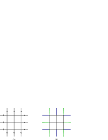
Figure 2: The graph and boundary conditions to put square ice configurations in bijection with ASMs for $n=3$ and the corresponding boundary conditions for paths.

If we color the vertices alternately black and white, and, if we color the edges blue and green depending on the color of the initial vertices, then the rule of two edges in and two out becomes the requirement that each vertex lie on two blue edges and two green edges. As the old boundary conditions determined the orientation of each edge on the boundary, the new one determine its color. Specifically, the boundary edges alternate in color, as in Figure 2(b).

Because no vertex lies on more than two blue edges, we may start at a blue edge on the boundary and follow that edge into the graph. At each interior vertex, there are two blue edges; so there is only one way to leave the vertex while remaining on blue and not retracing the path. Eventually this path ends somewhere else along the boundary. Thus, the path associates the initial vertex with the final vertex. This applies to each boundary vertex lying on a blue edge, so these vertices are divided into pairs by the blue paths of the ASM.

By focusing on the boundary, we may ignore the square structure of the graph, and think only of the outer ring of vertices in their cyclic order. Although a square must be rotated by multiples of $\frac{\pi}{2}$, we may rotate the boundary a much smaller amount, and ask how many ASMs produce the new pairing. The central result of this paper is that there are as many ASMs with the new pairing as with the old one, as conjectured by Carl Bosley and Lukasz Fidkowski[BF]; in fact, we construct an explicit bijection: from each ASM, we construct a new one, with the blue pairing rotated one step clockwise. Absolute position does not matter: a pairing may have connected two corners of the square, but now connects vertices in the middles of sides.

By considering the green edges and the closed loops, Henry Cohn and James Propp [CP] refined this conjecture to the form that we prove here. The boundary edges alternate blue and green. Exactly as with the blue ones, the green edges start paths joining the other half of the boundary vertices. The construction causes the green pairing to rotate not clockwise, but counterclockwise. Because of these opposing rotations, we call the bijection gyration. If we start at an interior vertex, then there are two blue edges, which may be followed to produce two blue paths. Either they both terminate on the boundary, so have been considered in the discussion of pairings, or they rejoin producing a closed loop. While gyration turns some loops from one color to the other, the total number remains constant.

Section 2 defines ASMs and another equivalent representation, called a height function, for which gyration is particularly simple. Section 3 contains the statement of our theorem on the properties of gyration. In Section 4, we define gyration. In Section 5, we split gyration into two steps, which are useful because they have similar properties to gyration itself, but which violate the boundary conditions. Section 6 proves a lemma, which identifies monochromatic paths before and after the these half-steps of gyration. It is the key step. Section 7 combines the lemma with the boundary conditions to prove the theorem. In Section 8 we describe other contexts for gyration and state some open problems.

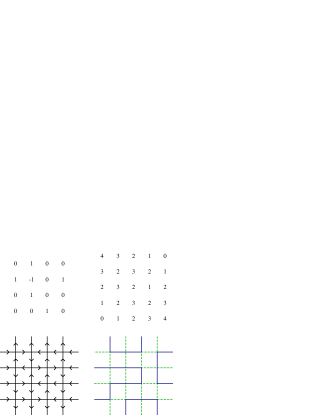
Figure 3: An ASM represented as a matrix, a square ice configuration, and a colored graph.

2 Relation to ASMs and Height Functions

An alternating sign matrix (ASM) of order $n$ is an $n\times n$ square matrix such that each entry is one of $1$, $-1$, and $0$, and the nonzero entries in each row and column alternate in sign and sum to $1$. Let ${\mathcal{A}}_{n}$ denote the set ASMs of order $n$. ASMs are in bijection with another class of matrix, called the corner sum matrix in [RR] and the skewed summation in [EKLP]. These are $(n+1)\times(n+1)$ matrices with integral entries such that horizontally and vertically adjacent entries differing by $1$ and the entries on the edge fixed at the values shown in Figure 3. See [RR] or [EKLP] for the specific bijection. We adopt the statistical mechanics term height function for this type of matrix. We will not make use of height functions, but we mention them because the simplest definition of gyration is in terms of height functions (see Section 4), and this definition can apply to many height functions. The entries of a height function matrix for an ASM should be thought of as ofset from the entries of the ASM itself. If the entries of the ASM lie on vertices in the square grid, then the entries of the height function lie on the faces of that graph.

We may choose the subgraph and some boundary conditions so that the set of configurations of square ice is in bijection with ASMs of order $n$ (see, e.g., [EKLP]). Take the $n^{2}$ vertices with both coordinates between $1$ and $n$, which are called interior vertices. Take all edges incident to these vertices; doing so requires that we take the $4n$ additional neighboring vertices, which have one coordinate from $1$ to $n$ and the other either $0$ or $n+1$; call these vertices endpoints. Denote this graph $L_{n}$. The interior vertices have degree $4$, and must be in one of the six vertex configurations, whereas the endpoints have degree $1$ and cannot. Instead, we require that the vertical edges incident to endpoints be directed out of the square and that the horizontal edges be directed in, as in Figure 2(a).

To turn a square ice configuration with such boundary conditions into an ASM, replace the vertical-out, horizontal-in vertices with $1$s, the vertical-in, horizontal-out vertices with $-1$s, and all other vertices with $0$s, as indicated in Figure 1. Since the four configurations that become $0$s have two horizontal edges oriented in the same absolute direction, the only way a line of horizontal edges, traversed from left to right, changes from edges pointing right to edges pointing left is by passing through a $1$; similarly, a change back comes from passing through a $-1$. Any vertex at which they do not change must come from a $0$. Consider two vertices in the same row that become nonzero and have only $0$s between them. All the edges between them must point in the same direction. The nonzero vertex in that direction is a $1$, and the other a $-1$. Thus the square ice model produces matrices with alternating nonzero entries. The boundary conditions require that the outermost nonzero entries both be $1$s; so the sum of the entries in a row is $1$. The vertical situation is similar, though the role of “in” and “out” switches, both in the configuration that becomes $1$ and in the boundary conditions.

If we give a vertex $(x,y)$ the same parity as $x+y$, and if we color blue those edges directed from odd to even and green those directed from even to odd, then we get a graph in which every interior vertex has two incident green edges and two incident blue edges, except the endpoints, which alternate in the color of their incident edges. In figures, we use solid and dashed lines to represent blue and green, respectively. Let us give an endpoint the same color as its incident edge. The six types of vertices in Figure 1 turn into the six types of vertices in Figure 4 in the same order if the vertex is odd. If the vertex is even, then 1(a) and 1(b) become 4(b) and 4(a), respectively. Similarly, c switches with d, and e with f. We can restore the square ice configuration by directing edges based on their color and the parities of their vertices; therefore, blue-degree $2$, green-degree $2$ graphs with the alternating boundary conditions are in bijection with square ice configurations with the vertical-out, horizontal-in boundary conditions, and thus with ASMs. Figure 3 shows an ASM represented as a matrix, as a square ice configuration, and as a colored graph.

Figure 4: The six vertex possibilities for vertices in the colored graph version of square ice.

In the subgraph of blue edges, all interior vertices have degree $2$, and the endpoints have lower degree; thus, the connected components of this graph are cycles, paths, and isolated points. The isolated points are the green endpoints and may be ignored at the moment. The blue endpoints are the only vertices of degree $1$, so all blue paths begin and end at two blue endpoints. We call the two endpoints of a monochromatic path paired, and refer to the partition of the endpoints into these pairs as the pairing of that ASM.

3 The Theorem

Carl Bosley and Lukasz Fidkowski [BF] conjectured a general principal, which we illustrate for order $3$. In the seven ASMs of order $3$, shown in Figure 5, each vertex is paired in three cases with its neighbor to the left, in three cases with its neighbor to the right, and once with the opposite vertex. Let us number the blue endpoints clockwise, starting with $(0,1)$. Then the observation is true for both vertex $1$, which is on a corner, and vertex $3$, which is in the middle of a side. In general, their conjecture was that from the perspective of the pairing data, the $2n$ blue endpoints are arranged not around a square, but at the vertices of a $2n$-gon: if they are rearranged by an element of $D_{2n}$, the number of ASMs pairing blue endpoints $i$ and $j$ remains the same. Henry Cohn and James Propp [CP] refined this conjecture to the form that we prove. This theorem, the central result of this paper, is stated below.

Figure 5: The blue edges in the seven ASMs of order $3$.

Theorem.

Let ${\mathcal{A}}_{n}(\pi_{B},\pi_{G},\ell)$ be the set of ASMs of order $n$ in which the blue subgraph induces pairing $\pi_{B}$, the green subgraph induces pairing $\pi_{G}$, and the sum of the number of cycles in the two subgraphs is $\ell$. If $\pi_{B}^{\prime}$ is $\pi_{B}$ rotated clockwise, and $\pi_{G}^{\prime}$ is $\pi_{G}$ rotated counterclockwise, then the sets ${\mathcal{A}}_{n}(\pi_{B},\pi_{G},\ell)$ and ${\mathcal{A}}_{n}(\pi_{B}^{\prime},\pi_{G}^{\prime},\ell)$ are in bijection.

The bijection of the theorem is given by gyration, which is defined in the next section. Since the blue and green endpoints rotate in opposite directions, we number the green endpoints clockwise by reflecting the blue labels over the line $y=x$. This labeling compensates for the opposite behavior of the two colors, so that the effect of $G$ is to induce the same permutation of the labels: an increase by $1$. In Section 5, we factor $G$ into two involutions, which have the same effect on the pairings as the generating reflections of $D_{2n}$. Thus if $\sigma\in D_{2n}$ is a permutation of the numbers from $1$ to $2n$ that induces $\pi_{B}^{\prime}$ by rearranging the labels from the pairing $\pi_{B}$ and similarly induces $\pi_{G}^{\prime}$ from $\pi_{G}^{\prime}$, then $|{\mathcal{A}}_{n}(\pi_{B},\pi_{G},\ell)|=|{\mathcal{A}}_{n}(\pi_{B}^{\prime},\pi_{G}^{\prime},\ell)|$.

4 Definition of Gyration

Recall that we represent an ASM as a coloring of the graph $L_{n}$, which lies in the square grid. The square grid is a planar graph and all of its faces are squares. Let us call the square with lower left corner $(i,j)$ even or odd according to the parity of $i+j$. Every edge in the grid is in one even and one odd square. To each square $S$ intersecting $L_{n}$, assign a function $G_{S}\colon{\mathcal{A}}_{n}\to{\mathcal{A}}_{n}$. In the height function representation of an ASM The function is given by fixing the color of all edges not in $S$ and determining the colors of the four edges in that square based solely on their original colors. If $S$ is on the boundary so that one or two of its edges are not in $L_{n}$, let $G_{S}$ be the identity. These boundary functions are not strictly necessary, but because they ensure that the even (or odd) squares that have functions cover $L_{n}$, they are a notational convenience in the next section. Otherwise, there are $2^{4}$, or $16$, possibilities for the colors of the four edges. In $14$ cases, two edges in the square incident to the same vertex are the same color. ASMs that have $S$ colored in one of these ways are fixed points of $G_{S}$. In the remaining cases, the four edges of $S$ are alternately blue and green; the two horizontal edges are one color, and the two vertical the other. For these two cases, the function reverses the color of all four edges. Since the only changes that $G_{S}$ makes is to switch these two cases, it is an involution.

In the square ice view of these objects, reversing the colors corresponds to reversing the direction of oriented edges. The involution reverses all four edges if and only if they are directed all clockwise or all counterclockwise about the square. In the ASM view, the involutions still have a local effect, switching between $0$s and $\pm 1$s, but the particular change and the decision to change depend on entries other than the four corresponding to the vertices of the square. The simplest description of $G_{S}$ is in terms of the height function representation, which is a matrix with entries offset from those in the ASM. Thus each entry lies on a square $S$ intersecting $L_{n}$. The matrix produced by $G_{S}$ agrees with the original matrix in every entry except possibly the one on $S$. There are at most two possible values that the entry on $S$ can take. If there is only one $G_{S}$ leaves the matrix unchanged. If there are two, $G_{S}$ changes the entry to be the other possibility.

Each $G_{S}$ may be considered to be “local” because it depends on and affects only a small set of edges. If $S$ and $S^{\prime}$ are distinct even (or odd) squares, then their edge sets are disjoint; moreover, $G_{S}$ and $G_{S^{\prime}}$ commute. Thus we may, without worry about order, define $G_{0}$ as the composition of the involutions of even squares, and $G_{1}$ as the composition of involutions of odd squares. Since they are compositions of commuting involutions, $G_{0}$ and $G_{1}$ are again involutions. Finally, we define $G$ by $G_{0}\circ G_{1}$.

Let’s summarize the definition: to perform a gyration on a graph, visit each unit square in the graph $L_{n}$, first the odd ones and then the even ones. In each visit, leave alone a square colored almost any way, but reverse the colors of all four edges if there are two parallel blue edges and two parallel green.

5 Alternative Decomposition

It will be convenient to form another decomposition $G=H_{0}\circ H_{1}$, where the $H_{k}$ are no longer functions ${\mathcal{A}}_{n}\to{\mathcal{A}}_{n}$, but affect the paths much like $G$. The range of $H_{1}$ and the domain of $H_{0}$ are no longer ${\mathcal{A}}_{n}$, but instead the similar set ${\mathcal{B}}_{n}$ of graphs with the same underlying graph and the same restriction on colors at vertices of degree $4$, but color-reversed boundary conditions. The blue endpoints alternate with the green ones, so gyration moves a blue endpoint two steps along, to the next blue one. By stopping between $H_{1}$ and $H_{0}$, we will find an intermediate place, where the blue path has moved halfway to its destination and ends at what we have labeled a green endpoint.

Because of the local nature of its definitions, $G_{S}$ may be given a larger domain and range, such as ${\mathcal{A}}_{n}\cup{\mathcal{B}}_{n}$ (or even all colorings). Then $G_{0}$ and $G_{1}$, defined by compositions, may also be extended to that domain. Let $R$ reverse the color of each edge. Since $G_{S}$ is symmetric in blue and green, it commutes with the $R$. Defined by composition, $G_{0}$ and $G_{1}$ also commute with $R$. Then define $H_{k}$, another involution, as the composition of $G_{k}$ with $R$. As $R^{2}$ is the identity, $H_{0}\circ H_{1}=G_{0}\circ G_{1}=G$.

Much as $G_{0}$ (respectively $G_{1}$) is the composition of local involutions associated with even (odd) squares, $R$ may be broken into the local reversals of even (odd) squares. Define $H_{S}$ as $G_{S}$ composed with the reversal of the colors of the edges of $S$, and define $H_{0}$ (respectively $H_{1}$) as the composition of the (commuting) $H_{S}$, for $S$ even (odd). Then $H_{S}$ preserves $2$ of the colorings of the edges of $S$ and reverses the colors in the other $14$. Figure 6 shows the effect of $H_{S}$ on $S$ for a complete (up to rotations) set of colorings of $S$.

From the perspective of this decomposition, the summary of $G$ becomes the following: to perform gyration, visit each unit square, in the same order as the previous description, and reverse the colors of the edges, if any two of the same color are incident to the same vertex, or some edge of the square is missing from $L_{n}$; if, instead, the four edges alternate blue and green around the square, then leave them unchanged.

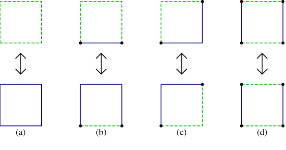
Figure 6: Examples of the effect of $H_{S}$ on the edges of $S$. Large vertices are fixed (see Section 6) with respect to the parity of the squares shown.

6 The Bijection of Components

Now that we have defined the $H_{k}$, we may begin to prove their properties. Fix a graph $c\in{\mathcal{A}}_{n}$ and $k\in\{0,1\}$. Call an interior vertex fixed if the unit squares of parity $k$ containing its two incident blue (or, equivalently, green) edges are distinct. The name is motivated by lemma below. The fixed vertices are the points where a monochromatic path moves from one square of parity $k$ to another. Fixed vertices provide the first suggestion that paths are well behaved under the application of $H_{k}$: a vertex is fixed in $c$ if and only if it is fixed in $H_{k}(c)$, as shown in Figure 6. This preservation also suggests the utility of fixed vertices; their drawback is that $H_{1-k}$ does not preserve them. Instead of focusing on the endpoints, which $H_{k}$ changes, it is easier to work with the fixed vertices, which stay the same, as is shown in the following lemma, which is the principal step in the proof of the theorem.

Lemma 1.

Two fixed vertices are in the same component of the blue (respectively green) subgraph after the action of $H_{k}$ if and only if they were in the same component of the blue (green) before.

Proof.

First consider distinct fixed vertices connected by a path of nonfixed vertices. Since fixed vertices are the points where paths move between squares of parity $k$, such a path must be contained in a single unit square of parity $k$; moreover, for a unit square to contain two fixed vertices, it must be contained in $L_{n}$ instead of being on the boundary. Figure 6 shows that, if there is a monochromatic path between two fixed vertices before the application of $H_{k}$, then there is one afterwards. Specifically, in two cases (Figure 6(a)), all four edges are the same color and there are no fixed vertices. In two cases (Figure 6(d) and a rotation), the edges alternate colors and there are four fixed vertices. In these cases, $H_{k}$ does not change the colors, so we may reuse the old path. In the remaining twelve cases (Figures 6(b), (c) and rotations), there are two fixed vertices connected by one blue and one green path. The application of $H_{k}$ switches these colors, leaving one path of each color.

As the endpoints have degree $0$ or $1$, they cannot be in paths connecting interior vertices, such as fixed vertices. Given a path between fixed vertices $v$ and $w$, we may divide it at each fixed vertex to obtain many paths of nonfixed vertices connecting fixed vertices. From such paths we may construct paths of nonfixed vertices connecting the intermediate fixed vertices after the application of $H_{k}$. Concatenating these paths, we produce a path connecting $v$ and $w$.

Since $H_{k}$ is an involution, the lemma in one direction implies the converse. ∎

The lemma allows us to identify the paths before and after the application of $H_{k}$. It proves that paths behave well and enables us to ask how they move. The involution changes the path, except at the fixed vertices, hence their name. The theorem makes more sense from this perspective: the paths remain intact, but their endpoints circulate, changing the pairing.

Fixed vertices record where paths moved between squares of a particular parity. Since the application of $H_{k}$ does not change whether a vertex is fixed, nor, as the lemma tells us, which path passes through that vertex, a path must pass through the same sequence of squares of parity $k$ before and after the application of $H_{k}$. All that may change is how the path moves inside each of those squares and what it does before the first fixed vertex and after the last. All that remains of the proof of the theorem is to see what happens in the initial and final segments between the endpoints and the fixed vertices.

7 Proof of the Theorem

Take a graph $c\in{\mathcal{A}}_{n}(\pi_{B},\pi_{G},\ell)$.

As the blue subgraph has maximum degree $2$, its components are paths, cycles, and isolated vertices. The lemma gives us a bijection between those blue components with fixed vertices before and after the application of $H_{k}$. A square of parity $k$, but not wholly contained in $L_{n}$, contains a blue endpoint, a green endpoint, a fixed vertex, and at most one nonfixed vertex. The fixed vertex is connected, by appropriately colored paths, to both endpoints. Thus every path connecting two blue endpoints contains at least one fixed vertex. Moreover, this fixed vertex is connected to the endpoints after $H_{k}$, so the bijection of components turns paths into paths and not into cycles.

Thus we have a bijection between the blue paths connecting endpoints before the application of $H_{k}$ with the blue paths connecting endpoints afterwards. We may compose the bijection induced by applying $H_{1}$ to $c$ with that induced by applying $H_{0}$ to $H_{1}(c)$ to obtain a bijection of the sets of blue paths in $c$ and $G(c)$. Since paths induce pairings of the endpoints, and we can associate a path in $c$ with a path in $G(c)$, we can associate the corresponding pairings of the endpoints of the two paths. All we need is to determine how the end of a path moves.

Recall that if a unit square of parity $k$ contains an endpoint, it is on the boundary of $L_{n}$ and it contains a fixed vertex and two endpoints, one blue and one green. When one of the $H_{k}$ affects that square, it switches the endpoints of the blue and green paths, leaving them both passing through the fixed vertex. For example, the unit square indexed by $(0,1)$ and affected by $H_{1}$ contains the blue endpoint $(0,1)$ and the green endpoint $(0,2)$. One of the vertices $(1,1)$ and $(1,2)$ is fixed, depending on whether the edge between them is green or blue, respectively. The effect of $H_{1}$ is to switch the endpoints, to make a blue path end at $(0,2)$ and a green path end at $(0,1)$. The endpoint of the blue path travels clockwise and the endpoint of the green path counterclockwise. Since there are two endpoints in each unit square on the boundary and the endpoints alternate colors, in each unit square the end of the blue path starts counterclockwise of the end of the green path and ends clockwise of it. Similarly, the unit squares associated with $H_{0}$ contain one endpoint of each color. They are arranged in the other order, with what is normally a blue endpoint clockwise of what is normally a green endpoint, but $H_{1}$ has already reversed the colors before the application of $H_{0}$. Thus $H_{0}$ also sends the blue paths clockwise and the green paths counterclockwise.

Over the course of the two steps of $G$, the end of a blue path moves two endpoints, or one blue endpoint, clockwise. Thus the label on each endpoint of a blue path increases by $1$. The effect on the pairing is the same as if we had relabeled the endpoints in that way. Since the endpoints move by switching blue and green, the green ones move counterclockwise, as was anticipated in the choice of green labels.

Finally, we must determine the number of closed loops of both paths in $G(c)$. The lemma states that $H_{k}$ turns cycles that contain fixed vertices into new cycles of the same color that contain fixed vertices; so the number of cycles of each color containing a fixed vertex is preserved. A cycle that does not contain a fixed vertex must be contained in a single unit square of parity $k$. Such a cycle reverses color; the total number of such cycles of both colors is preserved. Thus each $H_{k}$ preserves the total number of cycles; so must $G$, which is $H_{0}\circ H_{1}$. In addition, this preservation is bijective, although the division into cycles with fixed vertices and those without is not preserved because it depends on $k$.

The three statistics match the claims of the theorem, so we have the inclusion,

$$G({\mathcal{A}}(\pi_{B},\pi_{G},\ell))\subset{\mathcal{A}}(\pi_{B}^{\prime},\pi_{G}^{\prime},\ell).$$

The reverse inclusion can be obtained by a similar argument about $G^{-1}$ because $H_{0}$ and $H_{1}$ played essentially identical roles in the proof and $G^{-1}=H_{1}\circ H_{0}$.

To establish the dihedral version of the theorem, note that the function $d$ that reflects a graph across the line $y=x$ reverses the colors of the endpoints. Since $H_{1}$ and $H_{0}$ also reverse the colors of the endpoints, composing $d$ with either of them gives a function ${\mathcal{A}}_{n}\to{\mathcal{A}}_{n}$. Moreover, the reflection preserves the even and odd squares, so it commutes with $H_{1}$ and $H_{0}$. Thus $H_{k}d$ is an involution, and $G=H_{1}d\circ H_{0}d$. The effect of $H_{1}d$ is to send Endpoint $i$ to Endpoint $2n+1-i$, and $H_{0}d$ sends $i$ to $2n+2-i$ (modulo $2n$); in particular, $H_{0}d$ fixes $1$ and $n+1$. These two reflections generate $D_{2n}$. ∎

8 Generalizations and Conjectures

If $n<5$, then $G^{2n}$ is the identity. For larger $n$, it is a bijection ${\mathcal{A}}_{n}\to{\mathcal{A}}_{n}$, which preserves the three statistics, but which is not the identity. Its order is unknown in general. Table 1 shows that the order tends to be divisible by rather small primes, but this phenomenon is not surprising as the order is the least common multiple of the sizes of the orbits. A similar function is $G^{n}$ composed with rotation by $\pi$.

Table 1: The order of $G^{2n}$

$$\begin{array}[]{cc}\hline\cr\vskip 3.0pt plus 1.0pt minus 1.0pt\cr n&\textrm{order}\\ \hline\cr\vskip 6.0pt plus 2.0pt minus 2.0pt\cr 4&1\\ 5&2\\ 6&2\cdot 3\cdot 5\cdot 7\\ 7&2^{2}\cdot 3^{2}\cdot 5\cdot 7\cdot 11\cdot 19\\ \hline\cr\vskip 6.0pt plus 2.0pt minus 2.0pt\cr\end{array}$$

A torus graph with both dimensions even is bipartite, so the bijection between square ice and colored graphs remains. Such a torus graph has bipartite dual, allowing the division of the squares into even and odd, which allows the two steps of gyration. Gyration preserves the total number of cycles, but there are no paths to change. Much as with $G^{2n}$ on the square, we ask for the order of gyration on the torus. Similarly, gyration is well defined and nicely behaved on the infinite plane, although counting is more difficult and statistics may not be defined.

Bijections similar to gyration may be constructed on many models that have a height function, though the representation in terms of colored paths is lost and with it the theorem. Mills, Robbins, and Rumsey examined involutions analogous to $G_{0}$ and $G_{1}$ under the names $\rho$ and $\gamma$ [MRR83].

Knowing that certain sets are in bijection, we are led to ask for their cardinalities. Let $A_{n,k}$ be the number of ASMs of order $n$ such that the blue paths pair vertex $i$ with vertex $2k+1-i$ for $1\leq i\leq 2k$, so that there are nested paths $k$ deep. Let $B_{n,k}$ be those ASMs with that constraint and the additional requirement that for $i>k$, blue endpoint $2i$ is paired with blue endpoint $2i-1$. The author conjectures that $A_{n,k}=B_{n+1,k+1}$. Equality holds for $1\leq n\leq 8$ and $0\leq k\leq 5$. In the cases $k=0,1$, the conjectures are due to James Propp and David Wilson [PW].

The case $k=0$ gives $A_{n,0}=B_{n+1,1}$, which is the most interesting case because both sides simplify. The set counted by the right-hand side is the same as that counted by $B_{n+1,0}$ because they both require that vertex $1$ pair with vertex $2$. The new name $B_{n+1,0}$ is more appealing than $B_{n+1,1}$ because it unifies all of the pairings under a fairly simple rule: every blue path connects consecutively numbered endpoints. The conjecture implies that this set is enumerated by $A_{n,0}$, which is the number of unrestricted ASMs, and is shown in [Z] and [K] to be $\prod_{i=0}^{n-1}\frac{(3i+1)!}{(n+i)!}$.

References

- [BF] Bosley, C. and Fidkowski, L., Personal Communication, 1998.
- [B] Bressoud, D., Proofs and Confirmations: The Story of the Alternating Sign Matrix Conjecture. Cambridge, England: Cambridge University Press, 1999.
- [CP] Cohn, H. and Propp, J., Personal Communication, 1998.
- [EKLP] Elkies, N., Kuperberg, G., Larsen, M., and Propp, J., Alternating-Sign Matrices and Domino Tilings, I, J. Algebraic Combin. 1 (1992), 111–132.
- [K] Kuperberg, G., Another proof of the alternating-sign matrix conjecture, Internat. Math. Res. Notices 1996 (1996), 139–150. arXiv:math.CO/9712207
- [MRR82] Mills, W. H., Robbins, D. P., and Rumsey, H., Jr., Proof of the Macdonald Conjecture, Inventiones Mathimaticae 66 (1982), 73–87.
- [MRR83] Mills, W. H., Robbins, D. P., and Rumsey, H., Jr., Alternating-sign matrices and descending plane partitions, J. Combin. Theory Ser. A 34 (1983), 340–359.
- [MRR86] Mills, W. H., Robbins, D. P., and Rumsey, H., Jr., Self-complementary totally symmetric plane partitions, J. Combin. Theory Ser. A 42 (1986), 277–292.
- [PW] Propp, J. and Wilson, D., Personal Communication, 1999.
- [RR] Robbins, D. P. and Rumsey, H., Jr., Determinants and alternating sign matrices, Adv. Math. 62 (1986), 169–184.
- [Z] Zeilberger, D., Proof of the alternating sign matrix conjecture, Electronic J. of Combinatorics 3(2) (1996), R13.