The Theta Divisor and the Casson-Walker Invariant

Abstract.

We use Heegaard decompositions and the theta divisor on a Riemannian surface to define a three-manifold invariant for rational homology three-spheres. This invariant is defined on the set of ${\mathrm{Spin}}^{c}$ structures

$$\widehat{\theta}\colon{\mathrm{Spin}}^{c}(Y)\longrightarrow\mathbb{Q}.$$

In the first part of the paper, we give the definition of the invariant (which builds on the theory developed in [18]). In the second part, we establish a relationship between this invariant and the Casson-Walker invariant.

1. Introduction

In [18], we studied a topological invariant associated to Heegaard decompositions of oriented three-manifolds whose first Betti number $b_{1}(Y)$ is positive. Starting with a Heegaard decomposition $U_{0}\cup_{\Sigma}U_{1}$ for $Y$, the invariant measures how the theta divisor of $\Sigma$ moves as the surface undergoes degenerations naturally associated to the Heegaard splitting. In this paper, we describe a related construction which works in the case where $b_{1}(Y)=0$, giving a function

$$\widehat{\theta}\colon{\mathrm{Spin}}^{c}(Y)\longrightarrow\mathbb{Q}$$

on the set of ${\mathrm{Spin}}^{c}$ structures on $Y$. Once again, the invariant measures how the theta divisor moves under the prescribed degenerations, except that now a subtlety arises due to a path-dependence of the earlier construction.

To recall the definition of the invariant from [18], we give some geometric background. A Heegaard decomposition $U_{0}\cup_{\Sigma}U_{1}$ of $Y$ is a decomposition of the three-manifold as a union of two handlebodies, identified along an oriented surface $\Sigma$ of genus $g$. A handlebody $U$ can be described by attaching to $\Sigma$ $g$ two-handles and one three-handle. Let $\{\gamma_{1},...,\gamma_{g}\}$ denote the attaching circles for these two-handles. As explained in [18], the handlebody gives rise to a special class of metrics on $\Sigma$, the $U$-allowable metrics. Informally, any metric which is sufficiently stretched out normal to $\{\gamma_{1},...,\gamma_{g}\}$ is a $U$-allowable metric. We think of the Jacobian, $J$, as the space of holomorphic line bundles over $\Sigma$ with degree $g-1$, which in turn is identified with $H^{1}(\Sigma;S^{1})$, by specifying a spin structure on $\Sigma$. The handlebody $U$ gives rise to a canonical $g$-dimensional torus $L(U)\subset J$, which corresponds to the torus $H^{1}(U;S^{1})\subset H^{1}(\Sigma;S^{1})$ under the correspondence induced from any spin structure on $\Sigma$ which extends to $U$. (Note that $L(U)$ is independent of the spin structure on $U$.) A metric $h$ on $\Sigma$ gives rise to an Abel-Jacobi map

$$\Theta\colon\mathrm{Sym}^{g-1}(\Sigma)\longrightarrow J,$$

which associates to a point $D$ in the $(g-1)$-fold symmetric product the holomorphic line bundle which admits a holomorphic section vanishing exactly at $D$. For a $U$-allowable metric, $L(U)$ is disjoint from the theta divisor. Fix a path $h_{t}$ such that $h_{0}$ is $U_{0}$-allowable and $h_{1}$ is $U_{1}$-allowable, and consider the moduli space

$$M(h_{t})=\{(s,t,D)\in[0,1]\times[0,1]\times\mathrm{Sym}^{g-1}(\Sigma)\big{|}s\leq t,\Theta_{h_{s}}(D)\in L(U_{0}),\Theta_{h_{t}}\in L(U_{1})\}.$$

For a generic path (and small perturbations of the $L(U_{0})$ and $L(U_{1})$), these points form a discrete set, which misses the locus where $s=t$. Moreover, the points can be naturally partitioned according to ${\mathrm{Spin}}^{c}$ structures over $Y$, and we define $\theta_{h_{t}}(\mathfrak{a})$ to be the signed number of points in the subset corresponding to the ${\mathrm{Spin}}^{c}$ structure $\mathfrak{a}$. When $b_{1}(Y)>0$, this signed count is shown to be independent of the path of metrics and, indeed, independent of the Heegaard decomposition used in its definition.

By contrast, in the case when $b_{1}(Y)=0$, the signed count $\theta_{h_{t}}$ depends on the choice of path $h_{t}$, since the moduli space can hit the locus where $s=t$ in a one-parameter family of paths. In order to get a well-defined topological invariant, we correct by certain rational-valued, metric-dependent correction terms. Specifically, the path of metrics $h_{t}$ can be used to construct a metric on the cylinder $\mathbb{R}\times\Sigma$ (where we stretch out the time directions, in a manner made precise in Section 5), and the path dependence of the invariant $\theta_{h_{t}}(\mathfrak{a})$ can be reinterpreted in terms of spectral flow: if $h_{t}$ and $h_{t}^{\prime}$ are two paths of metrics which connect $U_{0}$-allowable to $U_{1}$-allowable metrics, then the difference in the $\theta$ is related to the (complex) spectral flow of the ${\mathrm{Spin}}^{c}$ Dirac operator over the cylinder $\mathbb{R}\times\Sigma$ by:

$$\theta_{h_{t}^{\prime}}(\mathfrak{a})-\theta_{h_{t}}(\mathfrak{a})={\mathrm{SF}}(h_{t},h_{t}^{\prime})$$

(see Propositions 2.4 and 2.7). Over a handlebody $U$, in Section 3, we describe a canonical (integer-valued) correction term $\xi^{\circ}$ on the space of metrics over $U$ with $U$-allowable boundary, which also changes by spectral flow. Thus, if we take a path of metrics $h_{t}$, extend it over $U_{0}$ by $k_{0}$, and $U_{1}$ by $k_{1}$, we obtain a metric $k_{Y}$ over $Y$; and the quantity

$$\xi^{\circ}(k_{0})+\theta_{h_{t}}(\mathfrak{a})+\xi^{\circ}(k_{1})$$

will depend on the metric $k_{Y}$ only through the spectral flow of its associated Dirac operator, according to standard splitting results for the spectral flow. To get a topological invariant, then, it suffices to subtract off any other quantity which depends on the metric only through spectral flow in the same manner.

Such a canonical metric-dependent term $\xi_{k_{Y}}(\mathfrak{a})$ is furnished by the index theory for manifolds with cylindrical ends, developed by Atiyah-Patodi-Singer [2]. It is defined as follows. Choose any four-manifold $X$ bounding $Y$, equipped with a cylindrical-end metric $g_{X}$ and a ${\mathrm{Spin}}^{c}$ structure $\mathfrak{r}$ which bounds $k_{Y}$ and $\mathfrak{a}$ respectively. Then,

$$\xi_{k_{Y}}(\mathfrak{a})=\mathrm{ind}_{X}(\mbox{$\not\!\!D$})-\left(\frac{c_{1}(\mathfrak{r})^{2}-\sigma(X)}{8}\right),$$

where $\mathrm{ind}_{X}(\mbox{$\not\!\!D$})$ is the complex index of the Dirac operator associated to the ${\mathrm{Spin}}^{c}$ structure $\mathfrak{r}$, and $\sigma(X)$ is the signature of the intersection form of $X$. By the Atiyah-Singer index theorem, the correction term is independent of the choice of four-manifold $X$ and extending ${\mathrm{Spin}}^{c}$ structure $\mathfrak{r}$. Note that $\xi_{k_{Y}}(\mathfrak{a})$ is a priori a rational number (since $c_{1}(\mathfrak{r})^{2}$ is rational). (Equivalently, $\xi_{k_{Y}}(\mathfrak{a})$ can be obtained as a combination of APS eta-functions for the Dirac and signature operators – see Equation (24). This latter point of view is exploited in Section 8.)

We now define the normalized invariant $\widehat{\theta}$ by the equation

$$\widehat{\theta}(\mathfrak{a})=\xi^{\circ}(k_{0})+\theta_{h_{t}}(\mathfrak{a})+\xi^{\circ}(k_{1})-\xi_{k_{Y}}(\mathfrak{a}).$$

This construction parallels, and was motivated by, a similar treatment of the Seiberg-Witten invariant for homology three-spheres (see [9], [14], [7]).

Our first result, whose proof occupies Sections 2-4, is that the quantity $\widehat{\theta}$, whose definition involves certain choices (a Heegaard decomposition, a family of metrics, etc.), gives a well-defined three-manifold invariant:

Theorem 1.1.

The function

$$\widehat{\theta}\colon{\mathrm{Spin}}^{c}(Y)\longrightarrow\mathbb{Q}$$

is a well-defined topological invariant; in particular, it does not depend on the metrics, Heegaard decompositions of $Y$.

Moreover, we will work out a surgery formula for the invariant, which gives a relationship between $\widehat{\theta}$ and the invariant $\theta$ for manifolds with $b_{1}(Y)=1$. The surgery formula, and our previous computations of $\theta$ when $b_{1}(Y)=1$ from [18], give the following link between the complex geometry of the Heegaard decomposition and the $SU(2)$ representations of the fundamental group of $Y$:

Theorem 1.2.

Let $Y$ be an integral homology three-sphere. Then,

$$2~{}\widehat{\theta}(Y)=\lambda(Y),$$

where $\widehat{\theta}(Y)$ is the invariant evaluated on the unique ${\mathrm{Spin}}^{c}$ structure of $Y$, and $\lambda(Y)$ is Casson’s invariant normalized so that $4\lambda(Y)\equiv\mathrm{sign}(X)\pmod{16}$ for each spin four-manifold $X$ which bounds $Y$.

The surgery formula for integral homology three-spheres, and the proof of the above theorem, are given in Section 6. In Section 7, we study the $\widehat{\theta}$-invariant for rational homology three-spheres. The main result of that section gives a relationship between $\widehat{\theta}$ and Walker’s generalization of Casson’s invariant (see [21]):

Theorem 1.3.

Let $Y$ be a rational homology three-sphere. Then,

$$2\sum_{\mathfrak{a}\in{\mathrm{Spin}}^{c}(Y)}\widehat{\theta}(\mathfrak{a})=\big{|}H_{1}(Y;\mathbb{Z})\big{|}\lambda(Y),$$

where $\lambda(Y)$ is the Casson-Walker invariant of $Y$.

It is interesting to compare the above with the situation in gauge theory. Counting solutions to the Seiberg-Witten equation, one obtains a metric-dependent quantity for rational homology spheres, which depends on its metric through the spectral flow of the Dirac operator. This is the signed count $SW_{Y}(\mathfrak{a})$ of the irreducible Seiberg-Witten monopoles. This, too, can be corrected by the metric-dependent quantity $\xi_{k_{Y}}$ to obtain a rational-valued function

$$SW\colon{\mathrm{Spin}}^{c}(Y)\longrightarrow\mathbb{Q}.$$

Results of  [14] and [7] show that for integral homology three-spheres this invariant agrees with half of Casson’s invariant. This, together with Theorem 1.2, underlines the close relationship between $\widehat{\theta}$ and the Seiberg-Witten invariant (see also [18] for the case where $b_{1}(Y)>0$). In fact, we discovered the invariants $\theta$ and $\widehat{\theta}$ by studying Seiberg-Witten theory and Heegaard decompositions, and it is very natural to make the following conjecture:

Conjecture 1.1.

The invariant $\widehat{\theta}$ agrees with the Seiberg-Witten invariant $SW$ for all rational homology three-spheres.

There are two routes for establishing this conjecture: one is to compare the surgery formulas for both invariants, another is to proceed more directly via an adiabatic limit of the Seiberg-Witten equations. Carrying out either programme would take us rather far from the scope of the present paper. We hope to return to these topics in a future paper.

2. Definition of the Invariant

In this section, we start with studying the metric dependence of the quantity $\theta$, with a view to showing the topological invariance of $\widehat{\theta}$. We begin with a few preliminary remarks on the definition of $\theta$.

Definition 2.1.

A path $\{h_{t}\}_{t\in[0,1]}$ of metrics over $\Sigma$ is called $(U_{0},U_{1})$-allowable if the metric $h_{0}$ is $U_{0}$-allowable, and the metric $h_{1}$ is $U_{1}$-allowable.

Let $M(h_{t})$ denote the moduli space introduced in Section 1.

Proposition 2.2.

The moduli space $M(h_{t})$ can be naturally partitioned into components $M(h_{t},\mathfrak{a})$ labeled by ${\mathrm{Spin}}^{c}$ structures over $Y$. Moreover, for a generic $(U_{0},U_{1})$-allowable path of metrics $h_{t}$ on $\Sigma$, the moduli space is a compact, oriented $0$-manifold which does not contain any points with $s=t$.

Proof. The orientation and partitioning into ${\mathrm{Spin}}^{c}$ structures are described in Section LABEL:Theta:sec:DefTheta of [18]. When $g>1$, the genericity statement follows from Proposition 4.1, which is proved in Section 4 of the present paper. Note that solutions with $s=t$ correspond to points in $\mathrm{Sym}^{g-1}(\Sigma)$ which map to $L(U_{0})\cap L(U_{1})$, which is a discrete set of points (since $Y$ is a homology three-sphere); so these are excluded by dimension counting.

When $g=1$, it is easy to see that the moduli space is empty: in that case, the theta divisor consists of a single, isolated spin structure, which does not bound.         

Armed with Proposition 2.2, we can define $\theta_{h_{t}}(\mathfrak{a})$ to be the signed number of points in the component of $M(h_{t},\mathfrak{a})$.

Definition 2.3.

Given a pair of $(U_{0},U_{1})$-allowable paths $h_{t}$ and $h_{t}^{\prime}$, a $(U_{0},U_{1})$-allowable homotopy from $h_{t}$ to $h_{t}^{\prime}$ is a smooth, two-parameter family of metrics

$$H\colon[0,1]\times[0,1]\rightarrow\mathrm{Met}(\Sigma)$$

so that for each $t\in[0,1]$, $H(0,t)=h_{t}$ and $H(1,t)=h_{t}^{\prime}$, and for each $u\in[0,1]$ the path $t\mapsto H(u,t)$ is a $(U_{0},U_{1})$-allowable path.

We will drop the handlebodies from the notation when they are clear from the context. Since the space of $U_{i}$-allowable metrics is path-connected for $i=0,1$, see [18] (and the space of metrics over $\Sigma$ is simply-connected), any two $(U_{0},U_{1})$-allowable paths can be connected by a $(U_{0},U_{1})$-allowable homotopy.

Note that since $Y$ is a rational homology sphere, the ${\mathrm{Spin}}^{c}$ structures naturally correspond to the intersection points of $L_{0}=L(U_{0})$ and $L_{1}=L(U_{1})$, see also [18].

Proposition 2.4.

Let $h_{t}$ and $h_{t}^{\prime}$ be a pair of generic $(U_{0},U_{1})$-allowable paths. Then,

$$\theta_{h_{t}}(\mathfrak{a})-\theta_{h_{t}^{\prime}}(\mathfrak{a})=\#\{(D,u,t)\in\mathrm{Sym}^{g-1}(\Sigma)\times[0,1]\times[0,1]\big{|}\Theta_{H(u,t)}(D)=p\},$$

where $H$ is any allowable homotopy from $h_{t}$ to $h_{t}^{\prime}$, and $p\in L_{0}\cap L_{1}$ is the point corresponding to the ${\mathrm{Spin}}^{c}$ structure $\mathfrak{a}$.

Remark 2.5.

Note that the set $\{(D,u,t)\in\mathrm{Sym}^{g-1}(\Sigma)\times[0,1]\times[0,1]\big{|}\Theta_{H(u,t)}(D)=p\}$ is not necessarily transversally cut out, as one can easily see by considering spin structures (by Serre duality, it is easy to see that if $p$ corresponds to a spin structure, then the local multiplicities are always even). Thus, the intersection number is to be interpreted by perturbing $p$ slightly.

Proof. Let $H$ be a generic allowable homotopy connecting $h_{t}$ and $h_{t}^{\prime}$. Consider the moduli space

$$M(H)=\left\{(D,u,s,t)|s\leq t,\Theta_{H_{u,s}}(D)\in L(U_{0}),\Theta_{H_{u,t}}(D)\in L(U_{1})\right\}.$$

According to the generic metrics result, Proposition 4.1, this space is an oriented one-manifold with boundary. Since $H$ is an allowable homotopy, the only boundary components are $u=0$, $u=1$ and $s=t$. Thus, counting boundaries, with sign and multiplicity, we get the result as stated.         

The difference term appearing above has another natural interpretation as a spectral flow on the cylinder $\mathbb{R}\times\Sigma$, inspired by work of Yoshida ([22], see also [13], [6]). An allowable path $h_{t}$ and a scale factor $\mu$ naturally induces a metric on the cylinder $\mathbb{R}\times\Sigma$ given by $(\mu dt)^{2}+h_{t}$, where we extend $h_{t}$ to all $t\in\mathbb{R}$ by requiring $h_{t}=h_{0}$ (resp. $h_{1}$) for $t\leq 0$ (resp. $\geq 1$). To describe the relevant spectral flow, we introduce some terminology.

Definition 2.6.

A connection $A$ on a spinor bundle $W$ over $Y$ is called reducible if the trace of its curvature (or, equivalently, the curvature induced on its determinant line bundle) vanishes.

On a rational homology sphere $Y$ equipped with a Riemannian metric, each ${\mathrm{Spin}}^{c}$ structure has a unique reducible connection (up to gauge).

Proposition 2.7.

Fix a ${\mathrm{Spin}}^{c}$ structure $\mathfrak{a}\in{\mathrm{Spin}}^{c}(Y)$. Let $h_{t}$ be an allowable path for some Heegaard decomposition of a rational homology sphere $Y$. Let $A$ be a reducible over $[0,1]\times\Sigma$ which extends to a reducible over $Y$ for the ${\mathrm{Spin}}^{c}$ structure $\mathfrak{a}$. Then, the Dirac operator coupled to $A$ acting on $L^{2}(\mathbb{R}\times\Sigma)$ is Fredholm. If for each $t\in[0,1]$, the theta divisor for $h_{t}$ misses the point corresponding to $\mathfrak{a}$, then for all sufficiently large $\mu$, the Dirac operator for the metric $(\mu dt)^{2}+h_{t}$ and reducible belonging to $\mathfrak{a}$ has no $L^{2}$ kernel over $\mathbb{R}\times\Sigma$. Moreover, let $H$ be an allowable homotopy from $h_{t}$, $h_{t}^{\prime}$ over $\Sigma$. Then, there is some $\mu_{0}\geq 0$ such that for all sufficiently large $\mu,\mu^{\prime}\geq\mu_{0}$, the spectral flow between the two induced Dirac operators on $\mathbb{R}\times\Sigma$ coupled to reducible connections obtained by restricting the reducibles in $\mathfrak{a}\in{\mathrm{Spin}}^{c}(Y)$ is given by

$${\mathrm{SF}}\left((\mu dt)^{2}+h_{t},(\mu^{\prime}dt)^{2}+h_{t}^{\prime}\right)$$

$$= \#\left\{(D,u,t)\in\mathrm{Sym}^{g-1}(\Sigma)\times[0,1]\times[0,1]\big{|}\Theta_{H(u,t)}(D)=p\right\},$$

where $p$ is the point in $J(\Sigma)$ corresponding to the ${\mathrm{Spin}}^{c}$ structure $\mathfrak{a}$.

The above is a special case of the more general result (Proposition 5.3), which is proved in Section 5.

Together, Propositions 2.4 and 2.7 show that $\theta_{h_{t}}(\mathfrak{a})$ depends on the family of metrics and ${\mathrm{Spin}}^{c}$ connection used on the cylinder only through the spectral flow of its Dirac operator. We call metric-dependent quantities which depend on the metric through only the spectral flow of its associated Dirac operator chambered metric invariants. We use $\theta$, together with another invariant $\xi^{\circ}$ for handlebodies, to construct a chambered invariant for certain metrics on $Y$. Note that an allowable path $h_{t}$ and extensions $k_{0}$ and $k_{1}$ of the metrics $h_{0}$ and $h_{1}$ over $U_{0}$ and $U_{1}$ respectively can be spliced together naturally to form a metric $(k_{0})\#(h_{t})\#(k_{1})$ over $Y$.

In Section 3, we construct a canonical chambered invariant $\xi^{\circ}$ for handlebodies of arbitrary genus, which is uniquely determined by an excision property, and a normalization condition which guarantees that $\xi^{\circ}(D^{3})=0$ for a non-negative sectional curvature metric on the three-disk (see Proposition 3.3 for a precise statement of the excision property). Strictly speaking, this function depends on the metric and a connection used on the spinor bundle over $U$, and an exact perturbation of a reducible connection over $U$. Thus, the expression $\xi^{\circ}(\mathfrak{a}|U_{i},k_{i},a_{i})$, denotes the invariant evaluated on the metric $k_{i}$ and the ${\mathrm{Spin}}^{c}$ connection obtained by restricting the reducible in $\mathfrak{a}$ to $U_{i}$, and perturbing by $a_{i}$, where $a_{i}$ is a one-form which is compactly supported in the interior of $U_{i}$. (This one-form is used to ensure that the kernel of the Dirac operator on the handlebody has no kernel, see Lemma 3.1.)

Splitting properties of spectral flow, then, show that the quantity $\xi^{\circ}(\mathfrak{a}|U_{0},k_{0},a_{0})+\theta_{h_{t}}(\mathfrak{a})+\xi^{\circ}(\mathfrak{a}|U_{1},k_{1},a_{1})$ depends on the metric $(k_{0})\#(h_{t})\#(k_{1})$ and the connections used only through the spectral flow of the associated Dirac operator, as described in the next proposition. To state the proposition properly, we must analyze the choices made in “splicing” metrics to obtain a metric on $Y$.

Given metrics $k_{0}$, $k_{1}$ on the handlebodies $U_{0}$ and $U_{1}$, and a path $h_{t}$ on $\Sigma$ which interpolates between the metrics on $\Sigma$ induced on the boundaries of $U_{0}$ and $U_{1}$, we can splice to obtain a metric on $Y$. The spliced metric requires three additional parameters: a scale $\mu$ to be used on the path of metrics $h_{t}$, and a pair of “neck-length” parameters which specify lengths of cylinders to be spliced before and after the middle neck. More precisely, the metric

$$(k_{0})\#_{T_{0}}\left((\mu dt)^{2}+h_{t}\right)\#_{T_{1}}(k_{1})$$

will denote the metric on $Y$ which is obtained by inserting cylinders $[0,T_{i}]\times\Sigma$ given the product metric $dt^{2}+h_{i}$ for $i=0,1$ between the handlebodies $U_{0}$ and $U_{1}$ and the cylinder $[0,1]\times\Sigma$ endowed with the metric $(\mu dt)^{2}+h_{t}$.

Proposition 2.8.

Fix a ${\mathrm{Spin}}^{c}$ structure $\mathfrak{a}\in{\mathrm{Spin}}^{c}(Y)$. Let $h_{t}$ be a generic $(U_{0},U_{1})$-allowable path. For a scale $\mu$ and necklength parameters $T_{0}$ and $T_{1}$, let $k_{Y}(\mu,T_{0},T_{1})$ denote the metric on $Y$ obtained by splicing

$$k_{0}\#_{T_{0}}\left(\left(\mu dt\right)^{2}+h_{t}\right)\#_{T_{1}}k_{1}.$$

Let $A(\mu,T_{0},T_{1})$ denote the corresponding reducible connections. Then, for generic, compactly supported one-forms $a_{0}$, $a_{1}$ in $U_{0}$ and $U_{1}$, the Dirac operator on $Y$ for the metric $k_{Y}(\mu,T_{0},T_{1})$ and connection $A(\mu,T_{0},T_{1})+a_{0}+a_{1}$ has no kernel, provided that $\mu$, $T_{0}$, and $T_{1}$ are sufficiently large. Moreover, suppose that $H$ is an allowable homotopy from $h_{t}$ to another allowable path $h_{t}^{\prime}$ which interpolates between metrics $k_{0}^{\prime}$ and $k_{1}^{\prime}$. Then, for generic compactly-supported one-forms $a_{0}$, $a_{0}^{\prime}$ and $a_{1}$, $a_{1}^{\prime}$ on $U_{0}$ and $U_{1}$ respectively we have that for all sufficiently large $\mu$ and necklength parameters $T_{0},T_{1}$ the spectral flow of the Dirac operator $\mbox{$\not\!\!D$}(\mu,T_{0},T_{1})$ for the metric $k_{Y}(\mu,T_{0},T_{1})$ and connection $A(\mu,T_{0},T_{1})+a_{0}+a_{1}$ to the Dirac operator $\mbox{$\not\!\!D$}^{\prime}(\mu,T_{0},T_{1})$ for the metric $k_{Y}^{\prime}(\mu,T_{0},T_{1})$ and connection $A^{\prime}(\mu,T_{0},T_{1})+a_{0}^{\prime}+a_{1}^{\prime}$ is given by

$${\mathrm{SF}}(\mbox{$\not\!\!D$}(\mu,T_{0},T_{1}),\mbox{$\not\!\!D$}^{\prime}(\mu,T_{0},T_{1}))$$

$$= \left(\xi^{\circ}(\mathfrak{a}|U_{0},k_{0}^{\prime},a_{0}^{\prime})+\theta_{h_{t}^{\prime}}(\mathfrak{a})+\xi^{\circ}(\mathfrak{a}|U_{1},k_{1}^{\prime},a_{1}^{\prime})\right)$$

$$-\big{(}\xi^{\circ}(\mathfrak{a}|U_{0},k_{0},a_{0})+\theta_{h_{t}}(\mathfrak{a})+\xi^{\circ}(\mathfrak{a}|U_{1},k_{1},a_{1})\big{)}.$$

Proof. The vanishing of the kernel follows from the vanishing of the kernel over the three pieces: $U_{0}$, $[0,1]\times\Sigma$, and $U_{1}$ respectively. Over the handlebodies the kernel vanishes for generic choices of $a_{0}$ and $a_{1}$ (this will be proved in Lemma 3.1). Over the cylinder, it vanishes for generic paths $h_{t}$, according to Proposition 2.7. Moreover, the spectral flow statement follows from the splitting principle, the chambered property of $\xi^{\circ}$, and the chambered property of $\theta$, which in turn follows from Proposition 2.4 together with Proposition 2.7.         

In the above proposition, the connection $A=A(\mu,T_{0},T_{1})+a_{0}+a_{1}$ has no kernel for generic $a_{0}$ and $a_{1}$. Thus, if we consider a four-manifold $X$, equipped with a cylindrical-end metric $g_{X}$ and ${\mathrm{Spin}}^{c}$ structure $\mathfrak{r}$ which bounds $k_{Y}$ and $\mathfrak{a}$ respectively, we can find a ${\mathrm{Spin}}^{c}$ connection ${\widetilde{A}}$ which $dt+A$ in a collar neighborhood of its boundary. According to [2], the Dirac operator coupled to ${\widetilde{A}}$ acting on $L^{2}(X)$ (given a cylindrical end $Y\times[0,\infty)$, and endowed with the natural extension of ${\widetilde{A}}$) is a Fredholm operator, and indeed the quantity

(1) $$\xi_{k_{Y}}(\mathfrak{a},A)=\mathrm{ind}_{X}(\mbox{$\not\!\!D$}_{\widetilde{A}})-\left(\frac{c_{1}({\widetilde{A}})^{2}-\sigma(X)}{8}\right),$$

where $\mathrm{ind}_{X}(\mbox{$\not\!\!D$})$ denotes the complex index of the Dirac operator, and $c_{1}({\widetilde{A}})$, of course, denotes the Chern-Weil representative of the first Chern class.

According to the above proposition, if we take the difference between $\xi^{\circ}(\mathfrak{a}|U_{0},k_{0},a_{0})+\theta_{h_{t}}(\mathfrak{a})+\xi^{\circ}(\mathfrak{a}|U_{1},k_{1},a_{1})$ and $\xi_{k_{Y}}(\mathfrak{a},A)$, we get a quantity which is independent of the extending metrics $k_{0}$, $k_{1}$ and the path $h_{t}$. In fact, we get something which is independent of the Heegaard decomposition as well, and hence a topological invariant of $Y$.

Theorem 2.9.

Let $h_{t}$ be a $(U_{0},U_{1})$-allowable path, and the $k_{Y}$ be the metric formed from $k_{0}$, $h_{t}$, and $k_{1}$, where $k_{i}\in\mathrm{Met}(U_{i})$ are metrics which bound $h_{0}$ and $h_{1}$ respectively. Then, for generic $a_{0}$ and $a_{1}$, the quantity

$$\widehat{\theta}(\mathfrak{a})=\xi^{\circ}(\mathfrak{a}|U_{0},k_{0},a_{0})+\theta_{h_{t}}(\mathfrak{a})+\xi^{\circ}(\mathfrak{a}|U_{1},k_{1},a_{1})-\xi_{k_{Y}}(\mathfrak{a},A)$$

(where $A=A(\mu,T_{0},T_{1})$ and $k_{Y}=k_{Y}(\mu,T_{0},T_{1})$ for sufficiently large $\mu$, $T_{0}$, and $T_{1}$) is a topological invariant of $Y$.

The independence of $\widehat{\theta}$ of the Heegaard decomposition relies on the corresponding result for $\theta$, which was established in [18]. To state the result, use a connected sum for paths of metrics. For a fixed metric on the torus $S^{1}\times S^{1}$, a metric $h$ over $\Sigma$ (which is flat in a neighborhood of the connected sum point $p\in\Sigma$), and a real number $T>0$, let $h(T)$ denote the metric on $\Sigma^{\prime}=\Sigma\#(S^{1}\times S^{1})$ obtained by a connected sum with neck-length $T$. Similarly, for a one-parameter family $h_{t}$ over $\Sigma$, we let $h_{t}(T)$ denote the one-parameter family of metrics on $\Sigma^{\prime}$ obtained in this manner. Then, we have the following:

Proposition 2.10.

Let $U_{0}\#_{\Sigma}U_{1}$ be a Heegaard decomposition of $Y$, and let $U_{0}^{\prime}\#_{\Sigma^{\prime}}U_{1}^{\prime}$ be the “stabilized” Heegaard decomposition; i.e. $U_{0}^{\prime}=U_{0}\#(S^{1}\times D)$, $\Sigma^{\prime}=\Sigma\#(S^{1}\times S^{1})$, $U_{1}^{\prime}=U_{1}\#(D\times S^{1})$. For a path of metrics on $h_{t}$ and a neck-length $T$, let $h_{t}(T)$ denote the path of metrics on $\Sigma^{\prime}$ obtained by forming the connected sum of metrics. Given a generic $(U_{0},U_{1})$-allowable path $h_{t}$, for all sufficiently large $T$, $h_{t}(T)$ is a generic $(U_{0}^{\prime},U_{1}^{\prime})$-allowable path, and the moduli spaces are diffeomorphic. Thus,

$$\theta_{h(T)}(\mathfrak{a})=\theta_{h_{t}(T)}(\mathfrak{a}).$$

Proof. The allowability of $h_{t}(T)$ and diffeomorphism statement for $\theta$ were proved in Proposition LABEL:Theta:prop:Stabilization of [18]; note that the hypothesis that $b_{1}(Y)>0$ was not used in the proof of this fact. One can arrange for $h_{t}$ and $h_{t}(T)$ to be generic simultaneously by varying the family $h_{t}$ in a region $U\subset\Sigma$ which does not contain the connected sum point. This statement is proved in Proposition 4.1.         

The proof of Theorem 2.9 is not difficult, given the excisive properties of spectral flow, and the above proposition. However, spelling out the precise form of excision needed involves some notation which we give in the Section 3, so we defer the proof to the end of that section.

3. Chambered metric invariants over Handlebodies

Let $Y$ be a closed, oriented three-manifold equipped with a ${\mathrm{Spin}}^{c}$ structure $\mathfrak{a}$ with spinor bundle $W$ whose first Chern class is torsion. Consider the space $\mathcal{C}(Y)$ of pairs $(k_{Y},A)$, where $k_{Y}$ is a metric over $Y$, and $A$ is a connection over $W$ (modulo gauge). This space is homotopy equivalent to the torus $\mathbb{T}^{b_{1}(Y)}$. A function

$$f\colon\mathcal{C}(Y)-\{(k,A)\big{|}\mathrm{Ker}\mbox{$\not\!\!D$}_{(k,A)}\neq 0\}\longrightarrow\mathbb{R}$$

is said to be a chambered metric invariant if

$$f(k_{Y}^{\prime},A^{\prime})-f(k_{Y},A)={\mathrm{SF}}(\mbox{$\not\!\!D$}_{(k_{Y},A)},\mbox{$\not\!\!D$}_{(k_{Y}^{\prime}A^{\prime})}),$$

where ${\mathrm{SF}}((k_{Y},A),(k_{Y}^{\prime},A^{\prime}))$ denotes the spectral flow of the ${\mathrm{Spin}}^{c}$ Dirac operator along any path in $\mathcal{C}(Y)$ which connects the pairs $(k_{Y},A)$ and $(k_{Y}^{\prime},A^{\prime})$; i.e. it is the intersection number of the spectrum of the ${\mathrm{Spin}}^{c}$ Dirac operator with the zero eigenvalue. Note that, since we have assumed that $c_{1}(W)$ is torsion, the Atiyah-Singer index theorem guarantees that the spectral flow is independent of the path.

Note that a chambered invariant is uniquely determined by its value on any one pair $(k_{Y},A)$ over $Y$. The quintessential chambered invariant is the invariant $\xi_{k_{Y}}$ defined by Equation (1). Our goal in this section is to construct a chambered metric invariant for handlebodies. When working with manifolds-with-boundary, special care must be taken to ensure that the spectral flow used in the above definition makes sense.

Let $U$ be a handlebody which bounds $\Sigma$, and fix an identification $\partial U\cong\Sigma$. Let $h$ be a metric on $\Sigma$. A metric $k$ is said to bound h if there is a neighborhood of $\partial U$ which is isometric to $(-1,0]\times\Sigma$ given the product metric

$$(dt)^{2}+h.$$

Note that a metric $k$ which bounds a metric on $\Sigma$ can be naturally extended to a cylindrical-end metric on the handlebody

$$U^{+}=U\cup_{\Sigma}\left([0,\infty)\times\Sigma\right).$$

A metric $k$ is said to be product-like near its boundary if it bounds some metric $h$ on its boundary. The relevant properties of the Dirac operator coupled to such a metric are summarized in the following:

Lemma 3.1.

Let $k$ be a metric on $U$ which bounds a $U$-allowable metric. Then for all connections $A$ on the spinor bundle of the form $A=A_{0}+a$, where $A_{0}$ is reducible and $a$ is compactly supported, the associated Dirac operator is Fredholm. Moreover, for generic such $A$, the associated Dirac operator has no kernel.

Proof. The connection $A$ naturally induces a connection on the spinor bundle of the boundary. More precisely, under the splitting

$$W|\partial U=S^{+}\oplus S^{-}$$

into the $\pm 1$-eigenspaces of Clifford multiplication by $i$ times the volume form of $\Sigma=\partial U$, the connection $A$ naturally induces a connection $B$ on $S^{+}$. If $\mathrm{Tr}F_{A}$ is compactly supported in $U$, then the induced connection $B$ has normalized curvature form.

The Dirac operator in a neighborhood of $\partial U$ takes the form

$$\frac{\partial}{\partial t}+\sqrt{2}\left(\begin{array}[]{cc}0&\overline{\partial}_{B}\\ \overline{\partial}_{B}^{*}&0\end{array}\right)\colon\left(\begin{array}[]{c}S^{+}\\ S^{-}\end{array}\right)\longrightarrow\left(\begin{array}[]{c}S^{+}\\ S^{-}\end{array}\right).$$

According to Proposition 1.1 of [2], this operator is Fredholm if the kernels of $\overline{\partial}_{B}$ and $\overline{\partial}_{B}^{*}$ are trivial. Now, if $A$ is reducible, or even if it differs from a reducible by a compactly supported one-form, then $B\in L(U)$. Thus, the Fredholm condition is guaranteed if $k$ is $U$-allowable.

The genericity statement is an application of the Sard-Smale theorem (see [19]). Let

$$\mathcal{C}^{\circ}(U)=\left\{(k,A+a)\Bigg{|}\begin{array}[]{l}\text{$k$ bounds a $U$-allowable metric}\\ \mathrm{Tr}F_{A}=0\\ a\in\Omega^{1}_{c}(i\mathbb{R})\end{array}\right\},$$

and

$${\mathfrak{M}}=\{(k,A,\Psi)\big{|}(k,A+a)\in\mathcal{C}^{\circ}(U),\mbox{$\not\!\!D$}_{k,A}\Psi=0,\|\Psi\|=1\}/\mathrm{Map}(U,S^{1}).$$

With in Sobolev completions, ${\mathfrak{M}}$ is a Banach manifold which is transversally cut out from

$$\mathcal{C}^{\circ}(U)\times\{\Psi\big{|}\|\Psi\|=1\}/\mathrm{Map}(U,S^{1})$$

by the Dirac equation: i.e. if $\phi$ were in its cokernel at $(k,A,\Psi)$, then by varying the spinor component, we would see that $\phi$ is $\mbox{$\not\!\!D$}_{(k,A)}$-harmonic. By varying the connection (indeed, in any open set), we see that $\phi$ must vanish identically (by the unique continuation principle). It is easy to see that the projection map from ${\mathfrak{M}}$ to $\mathcal{C}^{\circ}(U)/\mathrm{Map}(U,S^{1})$ which forgets the spinor is Fredholm of index $-1$. It follows then from the Sard-Smale theorem that for generic $(k,A)\in\mathcal{C}^{\circ}(U)$, there are no harmonic spinors.         

The above lemma gives a space $\mathcal{C}^{\circ}(U)$ of pairs $(k,A)$ for which the associated Dirac operator is a self-adjoint, Fredholm operator. Thus, as in [4], the spectral flow along any path in $\mathcal{C}^{\circ}(U)$ is well-defined. Indeed, since the ${\mathrm{Spin}}^{c}$ structure on a handlebody comes from a spin structure, and $\mathcal{C}^{\circ}(U)$ retracts back to the space of flat connections modulo gauge, the spectral flow of the Dirac operator between any two pairs in $\mathcal{C}^{\circ}(U)$ is well-defined and independent of the path joining them. (It is proved in Lemma LABEL:Theta:lemma:SFHandlebody of [18] that the spectral flow around any loop in the space of flat connections over the handlebody is trivial.) Thus, a function

$$f\colon\mathcal{C}^{\circ}(U)-\{(k,A)\big{|}\mathrm{Ker}\mbox{$\not\!\!D$}_{(k,A)}\neq 0\}\longrightarrow\mathbb{R}$$

is said to be a chambered invariant if

$$f(k^{\prime},A^{\prime})-f(k,A)={\mathrm{SF}}(\mbox{$\not\!\!D$}_{k,A},\mbox{$\not\!\!D$}_{k^{\prime},A^{\prime}}).$$

The goal of this section is to define one canonical chambered invariant $\xi^{\circ}$ for handlebodies of arbitrary genus, as we describe shortly. We then spell out the properties of this invariant. These results rely on a splitting theorem for spectral flow for manifolds with boundary, which in turn holds because we have a strong non-degeneracy condition along corners and boundaries: in the form which we require, the splitting principle can be seen to be a straightforward consequence of the Fredholm theory developed by Müller [17]. After proving the various properties of $\xi^{\circ}$, we use them to establish the stabilization invariance of the normalized invariant $\widehat{\theta}$, see Theorem 2.9.

To state the defining properties for $\xi^{\circ}$, we must describe how to (metrically) perform surgeries on a handlebody. (Figure 1 gives a schematic illustration of this operation in the case where the handlebody has genus two.) Let $U$ be a handlebody. Fix a collection of disjoint, embedded disks $\{D_{1},...,D_{n}\}\subset U$ (whose boundaries are embedded in the boundary of $\partial U$). A metric $k$ on $U$ which is product-like in a neighborhood of its boundary is said to be product-like in a neighborhood of the disks if there is an isometry from the metric product

$$\coprod_{i=1}^{n}D_{i}\times[-1,1]\subset U,$$

which identifies the central slice $D_{i}\times\{0\}$ with the $i^{th}$ disk, and where the disks $D_{i}$ are endowed with a non-negative scalar curvature metric which is product-like near its boundary. For positive real numbers $T_{1},...,T_{n}$, let $k(T_{1},...,T_{n})$ denote the metric stretched out normal to the disks: it is the metric obtained by replacing the cylinder $D_{i}\times[-1,1]$ with the elongated cylinder $D_{i}\times[-T_{i},T_{i}]$. Moreover, we say that the connection $A$ is product-like in a neighborhood of the disks $\{D_{1},...,D_{n}\}$ if the trace of its curvature vanishes in the product neighborhood and it is supported away from $\partial U$. In this case, the connection has a canonical extension $A(T_{1},...,T_{n})$ over the stretched out handlebody.

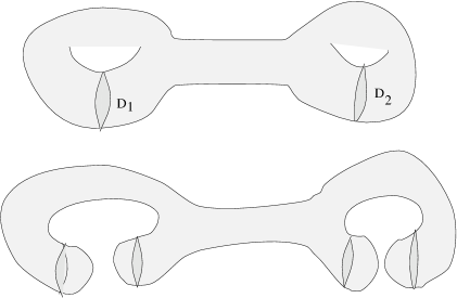
Figure 1. Surgeries on a genus $2$ handlebody

Given a genus $g$ handlebody $U^{g}$, one can find $g$ embedded disks $\{D_{1},...,D_{g}\}$, whose complement in $U^{g}$ is homeomorphic to a three-dimensional ball. Such a collection $\{D_{1},...,D_{g}\}$ is called a complete set of attaching disks for $U^{g}$. Note that if a metric $k$ bounds a metric $h$ on its boundary, and is product-like in a neighborhood of a complete set of attaching disks, then for all sufficiently large $T_{1},...,T_{g}$, the metric $k(T_{1},...,T_{g})$ is $U^{g}$-allowable in a neighborhood of its boundary. (Indeed, much of this section is modeled on the corresponding results for $U$-allowable metrics in Section 2 of [18].)

The complement $V$ of the attaching disks in $U^{g}$ is, strictly speaking, a manifold-with-corners. We smooth out the corners to get a smooth genus zero handlebody as follows. Let $B^{+}$ be the three-dimensional manifold-with-corners which is diffeomorphic to half of the three-dimensional ball (i.e. $B^{+}\cong\{(x,y,z)\in\mathbb{R}^{3}\big{|}x^{2}+y^{2}+z^{2}\leq 1,z\geq 0$). This manifold has two boundary components $\partial_{0}B^{+}$, $\partial_{1}B^{+}$, both of which are two-dimensional disks, which meet normally along their equator. The manifold obtained by attaching $2g$ copies of $B^{+}$ to $V$ along its $2g$ faces is a smooth, genus zero handlebody.

If $k$ is a metric on $U^{g}$ which is product-like in a neighborhood of the $g$ attaching disks, the genus zero handlebody inherits a metric which depends on $g$ parameters, denoted $k_{0}(T_{1},...,T_{g})$. This metric depends also on a choice of a metric $k_{0}^{+}$ on $B^{+}$ of non-negative sectional curvature, which in a neighborhood of both of its boundaries is isometric to $D\times[0,\epsilon)$. We construct such a metric in Lemma 3.2. Given this result, we let $k_{0}(T_{1},...,T_{g})$ denote the metric obtained by removing $(-1,1)\times D_{i}$ (for $i=1,...,g$) from $U^{g}$, attaching solid cylinders $[0,T_{i}]\times D$ along the $2g$ new boundary components, and then capping off with $2g$ copies of $B^{+}$, endowed with the metric $k_{0}^{+}$. Formally, $k_{0}(T_{0},...,T_{g})$ is the metric inherited from the description:

$$\Big{(}U^{g}-\bigcup_{i=1}^{g}[-1,1]\times D_{i}\Big{)}\cup_{\{\pm 1\}\times D_{i}=\{0\}\times D}\Big{(}\left[0,T_{i}\right]\times D\Big{)}\cup_{\{T_{i}\}\times D=\partial_{1}B_{\pm i}}\Big{(}B_{\pm i}\Big{)},$$

where $B_{\pm i}$ are $2g$ copies of $B^{+}$. Note that $k_{0}(T_{1},...,T_{g})$ is a metric on the genus zero handlebody (i.e. a three-ball), which is product-like near its boundary.

Moreover, if we have a ${\mathrm{Spin}}^{c}$ connection $A$ on $U^{g}$ which is product-like in a neighborhood of the disks, then it has a natural extension to the surgered manifold, obtained by extending it over the three-balls $B^{+}$ to have traceless curvature. We denote the resulting connection by $A_{0}(T_{1},...,T_{g})$. Before stating the definition of $\xi^{\circ}$, we pause to construct the metric $k_{0}^{+}$ on the three-dimensional half-ball used in the above construction.

Lemma 3.2.

There is a metric $k_{0}^{+}$ on $B^{+}$ with everywhere non-negative sectional curvatures, which is product-like in a neighborhood of its boundaries, and whose boundary is a union of two copies of $D$, meeting at a corner.

Proof. Fix some constant $0\leq\epsilon<\frac{1}{4}$, and fix a smooth, non-decreasing function

$$\psi\colon[0,1]\longrightarrow[0,1]$$

with

$$\psi(t)=\left\{\begin{array}[]{ll}\frac{3\epsilon}{2}&{\text{if $t\leq\epsilon$}}\\ t&{\text{if $t\geq 2\epsilon$}}\end{array}\right.$$

Then, the hypersurface

$$S^{3}\cong\{(x_{1},x_{2},x_{3},x_{4})\in\mathbb{R}^{4}\big{|}\sum_{i=1}^{4}\psi(x_{i})^{2}=1\}$$

inherits a metric from $\mathbb{R}^{4}$. The region where $x_{3}\geq 0$ and $x_{4}\geq 0$ is diffeomorphic to half of the three-ball (its two boundaries, are the loci where $x_{3}$ and $x_{4}$ vanish respectively). Since the function $\psi$ is constant for small values, the metric is easily seen to respect the corners. Moreover, the metric is easily seen to have all non-negative sectional curvatures (see for example [8]), as the hypersurface is locally described as a graph of $\sqrt{1-\psi(x_{1})^{2}-\psi(x_{2})^{2}-\psi(x_{3})^{2}}$ (after possibly renumbering the four variables), which is clearly a convex function.         

By doubling the metric $k_{0}^{+}$ above, we obtain a cylindrical-end metric on the three-ball $D^{3}$ with non-negative scalar curvature (note that this can be connected to any “standard” cylindrical-end metric on the three-disk through metrics of non-negative scalar curvature).

Proposition 3.3.

There is a unique chambered invariant $\xi^{\circ}$ with the following properties:

1. If $g=0$, and we endow $U$ with the metric obtained by doubling $k_{0}^{+}$ (and a connection with traceless curvature), then $\xi^{\circ}(U)=0$.

2. If $g=1$ and we endow $U$ with a product metric of the form $S^{1}\times D$ (and a connection with traceless curvature), then $\xi^{\circ}(U)=0$.

3. If $(k,A)$ is product-like in a neighborhood of $g$ attaching disks, then

   $$\xi^{\circ}(k(T),A(T))=\xi^{\circ}(k(T^{\prime}),A(T^{\prime})),$$

   for all sufficiently large $T,T^{\prime}$.

4. If $(k,A)$ is product-like in a neighborhood of $g$ attaching disks, then

   (2) $$\xi^{\circ}(k(T),A(T))=\xi^{\circ}(k_{0}(T),A_{0}(T))$$

   for all sufficiently large $T$.

This invariant is additive for boundary connected sum, in the following sense. Let $U^{g_{1}}$ and $U^{g_{2}}$ be a pair of handlebodies, and fix points $p_{1}$ and $p_{2}$ in $\partial U^{g_{1}}$ and $\partial U^{g_{2}}$ respectively. Fix metrics $k_{1}$ and $k_{2}$ for which a neighborhood of the $p_{1}$ and $p_{2}$, are isometric to the standard piece $B^{+}-\partial_{1}B^{+}$. Then, we can form the “boundary connected sum”

$$U^{g_{1}}\#_{T}U^{g_{2}}=\left(U^{g_{1}}-B^{+}\right)\cup\left([-T,T]\times D\right)\cup\left(U^{g_{2}}-B^{+}\right).$$

This is a genus $g_{1}+g_{2}$ handlebody, endowed with a metric, denoted $k_{1}\#_{T}k_{2}$, which bounds the connected sum metric $\left(\partial U^{g_{1}}\right)\#_{T}\left(\partial U^{g_{1}}\right)$. Moreover, if $A_{1}$ and $A_{2}$ are connections whose curvature is traceless over the standard pieces, then the connections can be naturally extended, as well.

Proposition 3.4.

The invariant $\xi^{\circ}$ is additive under boundary connected sum, in the sense that for pairs $(k_{1},A_{1})$ and $(k_{2},A_{2})$ on $U^{g_{1}}$ and $U^{g_{2}}$, there is a $T_{0}>0$, so that for all $T\geq T_{0}$,

$$\xi^{\circ}((k_{1},A_{1})\#_{T}(k_{2},A_{2}))=\xi^{\circ}((k_{1},A_{1})\#_{T}(k_{0}^{+},A_{0}^{+}))+\xi^{\circ}((k_{2},A_{2})\#_{T}(k_{0}^{+},A_{0}^{+})),$$

where $(k_{0}^{+},A_{0}^{+})$ is a pair over $B^{+}$ where $k_{0}^{+}$ is as in Lemma 3.2, and $A_{0}^{+}$ has traceless curvature.

This invariant is compatible with the correction term $\xi$ for $S^{3}$ with its genus zero or one Heegaard decompositions, in the following sense:

Proposition 3.5.

Let $S^{3}=U_{0}\cup_{\Sigma}U_{1}$ be a standard genus zero or one Heegaard decomposition of $S^{3}$. Let $h_{t}$ be a path of metrics on the Heegaard surface (sphere or two-torus) $\Sigma$, and let $k_{0}$, $k_{1}$ be metrics over the genus zero or one handlebodies $U_{0}$ and $U_{1}$ which extend $h_{0}$ and $h_{1}$ respectively. Then,

$$\xi\big{(}(k_{0})\#(h_{t})\#(k_{1})\big{)}=\xi^{\circ}(k_{0})+\xi^{\circ}(k_{1}).$$

The construction of $\xi^{\circ}$, and the proof of its various properties, rests a splitting (or excision) principle for spectral flow, which we will presently outline. This excision principle involves degenerating the handlebodies normal to embedded disks, and the objects one encounters under such degenerations are manifolds-with-corners. Formally, we have the following:

Definition 3.6.

A truncated handlebody $V$ is a smooth three-manifold with corners which is homeomorphic to a handlebody, and whose codimension one boundary consists of a surface-with-boundary $F$, the bounding surface, and a collection of disjoint disks $\{D_{1},...,D_{n}\}$, the faces. The bounding surface $F$ meets the faces normally along the boundary.

Examples of truncated handlebodies include the product $D\times[0,1]$, the half-ball $B^{+}$, and the complement of a collection of embedded disks in the genus $g$ handlebody.

It is useful to describe the product structure near the boundaries of a truncated handlebody $V$ in detail. To cover the faces, we have a diffeomorphism

$$\Phi\colon\bigcup_{i=1}^{n}D_{i}\times(-1,0]\subset V$$

onto a neighborhood of this boundary region for $V$. In turn, a neighborhood of the boundary of the union of disks admits an identification

$$\phi\colon\bigcup_{i=1}^{n}(-1,0]\times S^{1}_{i}\longrightarrow\bigcup_{i=1}^{n}D_{i}.$$

The remaining boundary region for $V$ is a surface $F$ of genus zero with $n$ boundary circles, and we have a diffeomorphism

$$\Psi\colon F\times(-1,0]\subset V.$$

onto this boundary region. A neighborhood fo the boundary of $F$ admits an identification

$$\psi\colon\bigcup_{i=1}^{n}S^{1}_{i}\times(-1,0]\longrightarrow F.$$

We can require that all these identifications be compatible, in the sense that the following maps commute:

$$\begin{CD}\bigcup_{i=1}^{n}(-1,0]\times S^{1}_{i}\times(-1,0]@>{\phi\times{{\mathchoice{\rm 1\mskip-4.0mul}{\rm 1\mskip-4.0mul}{\rm 1\mskip-4.5mul}{\rm 1\mskip-5.0mul}}}}>{}>\bigcup_{i=1}^{n}D_{i}\times(-1,0]\\ @V{{{\mathchoice{\rm 1\mskip-4.0mul}{\rm 1\mskip-4.0mul}{\rm 1\mskip-4.5mul}{\rm 1\mskip-5.0mul}}}\times\psi}V{}V@V{\Phi}V{}V\\ (-1,0]\times F@>{\Psi}>{}>V\end{CD}.$$

A metric $\mu$ is said to be product-like in a neighborhood of its boundaries if the above identifications $\Phi,\Psi,\phi,\psi$ are all isometries, where the domains of the maps are all given product metrics (and their ranges are given metrics induced from $\mu$).

A truncated handlebody $V$ can be naturally completed to a three-manifold $V^{+}$ without boundary by attaching $[0,\infty)\times F$ along the bounding surface, solid cylinders $D_{i}\times[0,\infty)$ along the faces, and a region $[0,\infty)\times S^{1}_{i}\times[0,\infty)$ along the corners $\{S^{1}_{i}\}$. If a metric $\mu$ is product-like in a neighborhood of its boundaries, it can be naturally extended to a complete metric, by giving all these standard pieces product metrics in a compatible manner. In particular, this compatibility ensures that in the region

$$\left([0,\infty)\times F\right)\cup\left([0,\infty)\times S^{1}_{i}\times[0,\infty)\right),$$

the metric $\mu^{+}$ is isometric to a product of $[0,\infty)$ with the cylindrical completion of the bounding surface

$$F^{+}=F_{\partial F=\bigcup S^{1}_{i}}\bigcup S^{1}_{i}\times[0,\infty)$$

As always, we will consider the Dirac operator with respect to such a metric, coupled to a ${\mathrm{Spin}}^{c}$ connection $A$ with traceless curvature. Note that the connection $A$ can be naturally extended to a connection $A^{+}$ on $V^{+}$ in such a manner that the curvature remains traceless.

Definition 3.7.

The pair $(\mu,A)$ is said to be strongly non-degenerate on the boundary if the restriction $(\mu,A)$ to the bounding surface $F$ has trivial kernel with APS boundary conditions or, equivalently, if the induced Dirac operator induced on any of the attached slices $F^{+}\subset V^{+}$ has trivial $L^{2}$ kernel.

Note that there is another product region “at infinity”, the region

$$D^{+}\times[0,\infty)=\left(D_{i}\times[0,\infty)\right)\cup\left([0,\infty)\times S^{1}_{i}\times[0,\infty)\right).$$

The induced Dirac operator on these attached slices $D^{+}$ automatically has trivial $L^{2}$ kernel, since its kernel is naturally identified with the harmonic spinors on the two-sphere (see Proposition LABEL:Theta:prop:LTwoCohom of [18]).

In [17], Müller considers Dirac operators on manifolds-with-corners, which satisfy a certain non-degeneracy hypothesis along its corners (see also [15]). Specializing some of his results to the case of truncated handlebodies, we obtain a Fredholm and exponential decay result. To spell out the exponential decay result, let $V_{T}\subset V^{+}$ denote the subset obtained by attaching subsets $F\times[0,T]$, $[0,T]\times S^{1}_{i}\times[0,T]$, and $D_{i}\times[0,T]$ to $V$.

Proposition 3.8.

Let $V$ be a truncated handlebody. Suppose that $(\mu,A)$ is strongly non-degenerate on the boundary. Then, the Dirac operator coupled to $A^{+}$ induces a Fredholm operator on $L^{2}(V^{+})$. In particular, there is a real number $\epsilon>0$ with the property that the spectrum of the Dirac operator in the range $(-\epsilon,\epsilon)$ is discrete. Moreover, eigenvectors in this range enjoy an exponential decay property: there are constants $C,c>0$ with the property that for each $\lambda$-eigenvector $\Phi$ of $\mbox{$\not\!\!D$}_{A^{+}}$ for $\lambda\in(-\epsilon,\epsilon)$,

$$\int_{V^{+}-V_{T}}|\Phi|^{2}\leq Ce^{-cT}\int_{V^{+}}|\Phi|^{2}.$$

Proof. Both statements are proved in [17]: the Fredholm paramatrix is constructed in the proof of Proposition 2.8, and the exponential decay estimate is Proposion 2.19 of that reference.         

Given the Fredholm paramatrix and exponential decay, the usual splicing techniques give a splitting principle for spectral flow. Suppose that $V$, $V^{\prime}$ be a pair of truncated handlebodies, and let $\{D_{1},...,D_{n}\}$, $\{D_{1}^{\prime},...,D_{n}^{\prime}\}$ be a collection of (not necessarily all) faces in $V$ and $V^{\prime}$ respectively. Then, we can form a new truncated handlebody

$$V\#_{T}V^{\prime}=\left(V\right)\cup_{D_{i}=D_{i}\times\{-T\}}\left(\bigcup_{i=1}^{n}D_{i}\times[-T,T]\right)\cup_{D_{i}\times\{T\}=D_{i}^{\prime}}\left(V^{\prime}\right).$$

If $(\mu,A)$ and $(\mu^{\prime},A^{\prime})$ is are strongly non-degenerate pairs on $V$ and $V^{\prime}$, discrete spectrum and exponential decay considerations on the boundaries show that for all $T$ sufficiently large, the induced pair $(\mu,A)\#_{T}(\mu^{\prime},A^{\prime})$ is strongly non-degenerate on $V\#_{T}V^{\prime}$. Indeed, we have the following direct consequence of Proposition 3.8:

Proposition 3.9.

Let $(\mu_{t},A_{t})$ and $(\mu_{t}^{\prime},A_{t}^{\prime})$ be a pair of one-parameter families of strongly non-degenerate data on $V$ and $V^{\prime}$, then for all sufficiently long tube-lengths, the spectral flow of $V\#V^{\prime}$ is the sum of the spectral flows of the pieces. More precisely, if the kernels of the Dirac operators of $\mbox{$\not\!\!D$}_{(\mu_{0},A_{0})}$, $\mbox{$\not\!\!D$}_{(\mu_{1},A_{1})}$, $\mbox{$\not\!\!D$}_{(\mu_{0}^{\prime},A_{0}^{\prime})}$, $\mbox{$\not\!\!D$}_{(\mu_{1}^{\prime},A_{1}^{\prime})}$ are all trivial, then there is a real $T_{0}$ so that for all $T\geq T_{0}$, the kernels of $\mbox{$\not\!\!D$}_{(\mu_{0},A_{0})\#_{T}(\mu_{0}^{\prime},A_{0}^{\prime})}$ and $\mbox{$\not\!\!D$}_{(\mu_{1},A_{1})\#_{T}(\mu_{1}^{\prime},A_{1}^{\prime})}$ are trivial, and indeed

$${\mathrm{SF}}((\mu_{t},A_{t})\#_{T}(\mu_{t}^{\prime},A_{t}^{\prime}))={\mathrm{SF}}(\mu_{t},A_{t})+{\mathrm{SF}}(\mu_{t}^{\prime},A_{t}^{\prime}).$$

Having set up the splitting principle for spectral flow, we turn our attention to the existence and uniqueness for $\xi^{\circ}$:

Proof of Proposition 3.3. Suppose $g=0$. Let $k_{0}$ be a metric obtained by doubling $k_{0}^{+}$. Let $A_{0}$ be the connection on the corresponding spinor bundle with traceless curvature. Given any pair $\wp=(k,A)\in\mathcal{C}^{\circ}(U)$, define

$$\xi^{\circ}(\wp)={\mathrm{SF}}(\wp_{0}^{+},\wp),$$

where $\wp_{0}^{+}$ consists of the metric $k_{0}$ and the reducible connection $A_{0}$. This is by definition a chambered invariant. Hence we have existence and uniqueness when $g=0$.

Suppose now that $g>0$, and let $\wp=(k,A)\in\mathcal{C}^{\circ}(U)$ be a pair which is product-like in a neighborhood of $g$ attaching disks $\{D_{1},...,D_{g}\}$. First, we show that for all sufficiently large $T$ the right hand side of Equation (2) stabilizes. Let $V$ denote the truncated handlebody obtained by removing the product neighborhoods of the attaching disks from $U^{g}$. For generic $\wp$, the kernel of the Dirac operator on $V$ has no kernel (this follows from the Fredholm property from Proposition 3.8, together with the proof of Lemma 3.1), so, by the splitting principle for the zero-modes, there is a $T_{0}$ so that for all $T\geq T_{0}$, the right hand side of Equation (2) for $\xi^{\circ}(\wp)$ does not depend on $T$. So we let Equation (2) be the definition of $\xi^{\circ}(k(T),A(T))$. Using spectral flow, this specifies $\xi^{\circ}$ for any pair $(k,A)\in\mathcal{C}^{\circ}(U)$. We have to show that $\xi^{\circ}$ is independent of the choice of product-like metric we started with, and, indeed, the choice of attaching disks.

To this end, let $\wp=(k,A)$ and $\wp^{\prime}=(k^{\prime},A^{\prime})$ be product-like in a neighborhood of the same $g$ attaching disks. Then by the splitting principle for spectral flow, for all sufficiently large $T$

$${\mathrm{SF}}(\wp(T),\wp^{\prime}(T))={\mathrm{SF}}(\wp_{0}(T),\wp^{\prime}_{0}(T)).$$

It follows that $\xi^{\circ}$ is independent of the choice of initial $\wp$.

Next, we verify that the definition of $\xi^{\circ}$ is independent of the particular choice of attaching disks when $g>0$. Suppose that $\wp\in\mathcal{C}^{\circ}(U)$ is product-like normal to $g+1$ disks $D_{1}^{\prime},D_{1},D_{2},...,D_{g}$, so that $\{D_{1},...,D_{g}\}$ and $\{D_{1}^{\prime},D_{2},...D_{g}\}$ are both complete sets of attaching disks. We would like to show that the value of $\xi^{\circ}$ obtained by surgering out the first set is the same as that obtained by surgering out the second set. To see this, we prove that the invariant agrees with a quantity obtained by surgering out all $g+1$ disks simultaneously. More precisely, let $\wp_{0}(T^{\prime},T)$ denote the pair on the genus zero handlebody obtained by inserting a cylinder $[-T^{\prime},T]\times D$ about $D_{1}^{\prime}$ and surgering out the $\{D_{1},...,D_{g}\}$, and let $\wp_{0,0}(T^{\prime},T)$ denote the metric obtained by surgering all $g+1$ disks (using tubelength $T^{\prime}$ around $D_{1}^{\prime}$ and $T$ around all the others). Note that the pair $\wp_{0,0}(T^{\prime},T)$ lives on a union of two disjoint genus zero handlebodies. (See Figure 2 for an illustration.)

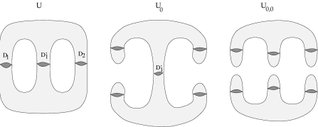
Figure 2. A genus $2$ handlebody $U$ with two complete sets of attaching disks $\{D_{1},D_{2}\}$ and $\{D_{1}^{\prime},D_{2}\}$. The manifold $U_{0}$ obtained by surgering along the first set of attaching disks is a three-ball, and the manifold $U_{0,0}$ obtained by surgering along all the attaching disks is a disjoint union of two three-balls.

By the splitting principle, the Dirac operator is generically invertible for all sufficiently long tubelengths (along all $g+1$ disks) in both $U$ and the doubly-surgered $U_{0,0}$. Thus, the quantity

$$Q={\mathrm{SF}}(\wp,\wp(T^{\prime},T))+{\mathrm{SF}}(\wp_{0,0}(T^{\prime},T),\wp_{0}^{+}\coprod\wp_{0}^{+})$$

is independent of the particular $T^{\prime},T$, provided that both are larger than some constant $T_{0}$. Our aim is to show that $Q$, in which both sets of attaching disks play the same role, agrees with $\xi^{\circ}$ calculated using the disks $\{D_{1},...,D_{g}\}$. We compare $Q$ with

$$P={\mathrm{SF}}(\wp,\wp(1,T))+{\mathrm{SF}}(\wp_{0}(1,T),\wp_{0}^{+}),$$

the quantity obtained by calculating $\xi^{\circ}$ using the disks $\{D_{1},...,D_{g}\}$. Now

$$P-Q = {\mathrm{SF}}(\wp(T^{\prime},T),\wp(1,T))+{\mathrm{SF}}(\wp_{0}(1,T),\wp_{0}^{+})+{\mathrm{SF}}(\wp_{0}^{+}\coprod\wp_{0}^{+},\wp_{0,0}(T^{\prime},T)).$$

But

$${\mathrm{SF}}(\wp_{0,0}(T^{\prime},T),\wp_{0}^{+}\coprod\wp_{0}^{+})={\mathrm{SF}}(\wp_{0}(T^{\prime},T),\wp_{0}^{+}),$$

since taking $T$ to be sufficiently large, both terms can be identified with the spectral flow from the complement of $D_{1}^{\prime}$ in $\wp_{0}(1,T)$ to the disjoint union of two half-balls $B^{+}\coprod B^{+}$ (endowed with the metric $k_{0}$ and connections with traceless curvature). Substituting back, we see that $P=Q$. Since we can switch the roles of $D_{1}$ and $D_{1}^{\prime}$ (without changing $Q$), we have shown that $\xi^{\circ}$ is independent of the attaching disks.

Note that $\xi^{\circ}(S^{1}\times D)$ is independent of the length of the $S^{1}$ factor, since the spectral flow between two such metrics vanishes. So, by definition $\xi^{\circ}(S^{1}\times D)$ agrees with the $\xi^{\circ}$ for the metric on $D^{3}$ obtained by surgering out the attaching disk. This metric is precisely $k_{0}^{+}\cup[-T,T]\times D\cup k_{0}^{+}$ – so $\xi^{\circ}$ of it vanishes. ∎

Proof of Proposition 3.4. The proof follows in the same manner as the proof that $\xi^{\circ}$ is independent of the attaching disks. Consider the attaching disks for $U^{g_{1}}$ and $U^{g_{2}}$, and the disk used for the boundary connected sum. Then pull out all $g_{1}+g_{2}+1$ disks simultaneously. ∎

Proof of Proposition 3.5. By the splitting theorem for spectral flow on the closed manifold $S^{3}$, we can reduce the proposition to a model case. Suppose that $k_{0}$, $h_{t}$, and $k_{1}$ are metrics on $U_{0}$, $\Sigma$, and $U_{1}$ for which the proposition is known, and let $k_{0}^{\prime}$, $h_{t}^{\prime}$, and $k_{1}^{\prime}$ denote arbitrary (compatible) metrics on $U_{0}$, $\Sigma\times[0,1]$, and $U_{1}$. Then,

$$\xi\left((k_{0}^{\prime})\#(h_{t}^{\prime})\#(k_{1}^{\prime})\right)-\xi\left((k_{0})\#(h_{t})\#(k_{1})\right) = {\mathrm{SF}}\left((k_{0})\#(h_{t})\#(k_{1}),(k_{0}^{\prime})\#(h_{t}^{\prime})\#(k_{1}^{\prime})\right)$$

$$= {\mathrm{SF}}(k_{0},k_{0}^{\prime})+{\mathrm{SF}}(h_{t},h_{t}^{\prime})+{\mathrm{SF}}(k_{1},k_{1}^{\prime}).$$

Note now that for $i=0,1$, ${\mathrm{SF}}\left(k_{i},k_{i}^{\prime}\right)=\xi^{\circ}(k_{i}^{\prime})-\xi^{\circ}(k_{i})$. Moreover, it follows from Proposition 2.7 that ${\mathrm{SF}}(h_{t},h_{t}^{\prime})\equiv 0$. Thus, the proposition is established once it is established for a model triple of metrics.

We consider the case where $g=1$. Let $k_{0}$ and $k_{1}$ be a pair of metrics the of the form $D\times S^{1}$, where the disk is endowed with a non-negative scalar curvature metric, and the $S^{1}$ factor has the same length as the boundary of $D$; let $h_{t}$ denote the constant family of metrics. We know that $\xi^{\circ}(k_{0})=\xi^{\circ}(k_{1})=0$, and need to show that for all sufficiently large $T$, $\xi(k_{0}\#_{T}k_{1})=0$.

We connect the standard, round metric on $S^{3}$ (for which it is easy to see that $\xi=0$, since it bounds a metric on the four-ball with non-negative sectional curvatures) with a metric of the form $k_{0}\#_{T}k_{1}$ through a path of metrics with non-negative scalar curvature, to show that the correction terms $\xi$ agree. To this end, let

$$\psi_{s}\colon[0,1]\rightarrow[0,1]$$

be a smooth, one-parameter family of smooth functions, depending smoothly on a parameter $s\in[0,1]$, with following properties:

• $\psi_{s}(t)=t$ for $t<1-s$,

• $\frac{\partial}{\partial t}\psi_{s}(t)\equiv 0$ for $t>1-s+\epsilon$,

• $\frac{\partial}{\partial t}\psi_{s}(t)\geq 0$ for all $t$,

• $\frac{d^{2}\psi_{s}}{dt^{2}}(t)\leq 0$ for all $t$.

For example, if $f\colon\mathbb{R}\rightarrow[0,1]$ is a smooth, non-increasing, non-negative function with $f(t)\equiv 1$ for $t<0$, $f(t)\equiv 0$ for $t>\epsilon$, then we can let $\psi_{s}(t)=\int_{0}^{t}f(x+s-1)dx$.

Let $(r,\theta,\phi)$ denote coordinates on $(0,1)\times S^{1}\times S^{1}$. The standard three-sphere can be obtained from this space by attaching two circles $0\times 0\times S^{1}$ and $1\times S^{1}\times 0$ “at infinity” (i.e. at $r=0$ and $r=1$). Moreover, for all $s<1$, the metric on $(0,1)\times S^{1}\times S^{1}$ given by

$$g_{s}=\frac{dr^{2}}{1-r^{2}}+\psi_{s}(r)^{2}d\theta^{2}+\psi_{s}(\sqrt{1-r^{2}})^{2}d\phi^{2}$$

extends over the two circles at $r=0$, $r=1$ to give a smooth metric on $S^{3}$, since in a neighborhood of those regions, $\psi_{s}(r)\equiv r$ and $\phi_{s}(\sqrt{1-r^{2}})\equiv\sqrt{1-r^{2}}$. Note that when $s=0$, the above metric agrees with the standard round metric on $S^{3}$. By Cartan’s method of moving frames (see [20]), it is easy to see that the connection matrix of the Levi-Civita connection is given by:

$$\left(\begin{array}[]{ccc}0&\sqrt{1-r^{2}}\psi_{s}^{\prime}(r)d\theta&-r\psi_{s}^{\prime}(\sqrt{1-r^{2}})d\phi\\ -\sqrt{1-r^{2}}\psi_{s}^{\prime}(r)d\theta&0&0\\ r\psi_{s}^{\prime}(\sqrt{1-r^{2}})d\phi&0&0\end{array}\right);$$

and hence the curvature matrix is:

$$\left(\begin{array}[]{ccc}0&-A(r)dr\wedge d\theta&-B(r)dr\wedge d\phi\\ A(r)dr\wedge d\theta&0&0\\ B(r)dr\wedge d\phi&0&0\end{array}\right),$$

where $A_{s}(r)=\frac{\psi_{s}^{\prime}(r)r}{\sqrt{1-r^{2}}}-\psi_{s}^{\prime\prime}(r)\sqrt{1-r^{2}}$ and $B_{s}(r)=\psi_{s}^{\prime}(\sqrt{1-r^{2}})-\frac{r^{2}\psi_{s}^{\prime\prime}(r)}{\sqrt{1-r^{2}}}$

Thus, the sectional curvatures are always non-negative.

When $s>\frac{1}{2}$, then $g_{s}$ extends to a decomposition of $S^{3}$ as a union of $S^{1}\times D$ with $D\times S^{1}$ endowed with the product metric. In particular, the metric is product-like in the region where $r$ is in a neighborhood of $\frac{1}{2}$.

Thus, the proposition follows. ∎

Proof of Theorem 2.9. In view of Proposition 2.8, the invariant $\widehat{\theta}(\mathfrak{a})$ can depend only on the Heegaard decomposition, not on the metrics used in its definition. Topological invariance then amounts to showing that $\widehat{\theta}(\mathfrak{a})$ remains unchanged under stabilization. But this is a consequence of the excision property of indices, together with the stabilization of $\theta(\mathfrak{a})$ (see Proposition 2.10).

Suppose $U_{0}\cup_{\Sigma}U_{1}$ is a Heegaard decomposition and

$$\left(U_{0}\#\left(S^{1}\times D\right)\right)\cup_{\Sigma\#\left(S^{1}\times S^{1}\right)}\left(U_{1}\#\left(D\times S^{1}\right)\right)$$

is its stabilization, then the difference $\Delta$ between the corresponding invariants $\widehat{\theta}$ (which we would like to show vanishes) is given by:

(3) $$\Delta = \xi^{\circ}\left(U_{0}\#_{T}\left(S^{1}\times D\right)\right)+\theta\left(h_{t}\#_{T}\left(S^{1}\times S^{1}\right)\right)+\xi^{\circ}\left(U_{1}\#_{T}\left(D\times S^{1}\right)\right)$$

$$-\xi\left(\left(U_{0}\#_{T}\left(S^{1}\times D\right)\right)\#\left(h_{t}\#_{T}\left(S^{1}\times S^{1}\right)\right)\#\left(U_{1}\#_{T}\left(D\times S^{1}\right)\right)\right)$$

$$-\xi^{\circ}\left(U_{0}\#_{T}B\right)-\theta\left(h_{t}\#_{T}\left(S^{2}\right)\right)-\xi^{\circ}\left(U_{1}\#_{T}B\right)$$

$$+\xi\left(\left(U_{0}\#_{T}B\right)\#\left(h_{t}\#_{T}\left(S^{2}\right)\right)\#\left(U_{1}\#_{T}\left(B\right)\right)\right).$$

Note that on $\Sigma\#(S^{1}\times S^{1})$ we are using an allowable path induced from an allowable path on $\Sigma$, as in Proposition 2.10; also on the handlebodies, we are using the metric arising from the boundary connected sum. The difference in the terms using $\xi$ is a spectral flow (by its chambered nature); moreover by the excision principle for spectral flow, we get:

$$\xi\left(\left(U_{0}\#_{T}\left(S^{1}\times D\right)\right)\#\left(h_{t}\#_{T}\left(S^{1}\times S^{1}\right)\right)\#\left(U_{1}\#_{T}\left(D\times S^{1}\right)\right)\right)$$

(4) $$-\xi\left(\left(U_{0}\#_{T}B\right)\#\left(h_{t}\#_{T}\left(S^{2}\right)\right)\#\left(U_{1}\#_{T}\left(B\right)\right)\right)$$

$$= {\xi\left(\left(B\#_{T}\left(S^{1}\times D\right)\right)\#\left(S^{2}\#_{T}\left(S^{1}\times S^{1}\right)\right)\#\left(B\#_{T}\left(D\times S^{1}\right)\right)\right)}$$

$$-\xi\left(\left(B\#_{T}B\right)\#\left(S^{2}\#_{T}\left(S^{2}\right)\right)\#\left(B\#_{T}\left(B\right)\right)\right)$$

$$= {\xi\left(\left(B\#_{T}\left(S^{1}\times D\right)\right)\#\left(S^{2}\#_{T}\left(S^{1}\times S^{1}\right)\right)\#\left(B\#_{T}\left(D\times S^{1}\right)\right)\right)}$$

i.e. we have excised out $Y$ and replaced it by a three-sphere (and used the positivity of the scalar curvature on the second term). Now, the compatibility of $\xi^{\circ}$ and $\xi$ (Proposition 3.5) allows us to conclude that

(5) $$\xi\left(\left(B\#_{T}\left(S^{1}\times D\right)\right)\#\left(S^{2}\#_{T}\left(S^{1}\times S^{1}\right)\right)\#\left(B\#_{T}\left(D\times S^{1}\right)\right)\right)$$

$$= \xi^{\circ}(B\#_{T}(S^{1}\times D))+\xi^{\circ}(B\#_{T}(D\times S^{1})).$$

Combining Equations (3), (4), and (5) (and using the additivity of $\xi^{\circ}$, see Proposition 3.4), we get that

$$\Delta=\theta(h_{t}\#(S^{1}\times S^{1}))-\theta(h_{t}\#(S^{2})).$$

By the stabilization invariance of $\theta$ (see Proposition 2.10), this implies that $\Delta=0$, as required. ∎

4. Transversality of the Theta Divisor

The aim of this section is to prove a “generic metrics” result for the Abel-Jacobi map. Indeed, we show that for a fixed divisor $D\in\mathrm{Sym}^{g-1}(\Sigma)$, the map from the space of metrics to the Jacobian

$$h\mapsto\Theta_{h}(D)$$

is a submersion onto the Jacobian, provided that the genus $g$ of the Riemann surface is greater than one. Strictly speaking, to view this as a map into one, fixed space, we fix a spin structure over $\Sigma$, and hence an identification $J_{h}\cong H^{1}(\Sigma;S^{1})$.

This technical result was used in our definition of $\theta$: it guarantees that the moduli space whose count defines $\theta$ does consist of isolated points. (It was also used in Section LABEL:Theta:sec:WallCross of [18], in the derivation of a “wall-crossing” formula.)

Proposition 4.1.

Let $\Sigma$ be a surface of genus greater than one. Then, for each divisor $D\in\mathrm{Sym}^{g-1}(\Sigma)$, the map

$$\mathrm{Met}(\Sigma)\longrightarrow H^{1}(\Sigma;S^{1})$$

given by $h\mapsto\Theta_{h}(D)$ is a submersion. Indeed, restricting to the subset of metrics which are fixed outside some open subset $U\subset\Sigma$, we still get a submersion.

The proof relies on the following elementary fact:

Lemma 4.2.

Given a pair of non-zero vectors $v,w\in\mathbb{R}^{2}$, and a complex structure $j_{0}$ on $\mathbb{R}^{2}$, i.e. an endomorphism of $\mathbb{R}^{2}$ with $j_{0}^{2}=-{{\mathchoice{\rm 1\mskip-4.0mul}{\rm 1\mskip-4.0mul}{\rm 1\mskip-4.5mul}{\rm 1\mskip-5.0mul}}}$, there is a one-parameter family $j_{t}$ of complex structures with $\frac{\partial}{\partial t}\Big{|}_{t=0}j_{t}v=w.$

Proof. We can introduce coordinates on $\mathbb{R}^{2}$ with respect to which $j_{0}$ takes the form $j_{0}=\left(\begin{array}[]{cc}0&-1\\ 1&0\end{array}\right)$. For any real numbers $a$, $b$, let $X=\frac{1}{2}\left(\begin{array}[]{cc}-b&-a\\ -a&b\end{array}\right)$. Clearly, $j_{t}(a,b)=e^{tX}j_{0}e^{-tX}$ gives a one-parameter family of complex structures whose differential at $t=0$ acts by

$$\left(\begin{array}[]{cc}-a&b\\ b&a\end{array}\right).$$

The lemma follows.         

Proof of Proposition 4.1. Suppose $h_{0}$ is some fixed metric, for which $\Phi$ is an $A_{0}$-holomorphic section which represents $D$. Then $\Theta_{h}(D)$ is defined as follows. Let $a^{0,1}\in\Omega^{0,1}_{h}$ be a form for which

$$\overline{\partial}_{A_{0}+a^{0,1}}\Phi=0.$$

Note that $a^{0,1}$ depends on the metric $h$. Then, $\Theta_{h}(D)=\Theta_{h_{0}}(D)+[\Pi_{\mathcal{H}_{h}}\mathrm{Im}a^{0,1}]$, where $\Pi_{\mathcal{H}_{h}}$ denotes the $L^{2}$ projection map to the space of harmonic one-forms $\mathcal{H}_{h}$ for the metric $h$. Now if the metric $h$ differs from $h_{0}$ only in a region $U\subset\Sigma$ where $\Phi\neq 0$, then $a^{0,1}$ can be written as follows:

$$a^{0,1}=-\frac{(1+iJ_{h})\nabla_{A_{0}}\Phi}{\Phi}.$$

Here, $J_{h}$ is (pull-back by) the almost-complex structure induced from the metric; i.e. it is the Hodge star operator on one-forms.

So, if $h_{t}$ is a one-parameter family of metrics through $t=0$ (where $\Phi$ is $A_{0}$-holomorphic), then the derivative of the theta map is given by

$$\frac{\partial}{\partial t}_{t=0}\left[\Pi_{\mathcal{H}_{h_{t}}}\mathrm{Im}\left(-\frac{(1+iJ_{h})\nabla_{A_{0}}\Phi}{\Phi}\right)\right] = \left[\Pi_{\mathcal{H}_{h_{0}}}\mathrm{Im}\left(i\frac{dh_{t}}{dt}(0)\frac{\nabla_{A_{0}}\Phi}{\Phi}\right)\right]$$

$$= \left[\Pi_{\mathcal{H}_{h_{0}}}J^{\prime}(0)\mathrm{Re}\left(\frac{\nabla_{A_{0}}\Phi}{\Phi}\right)\right].$$

Now, $b=\mathrm{Re}\left(\frac{\nabla_{A_{0}}\Phi}{\Phi}\right)$ is a differential one-form which cannot vanish identically: if it did, that would mean that $\Phi$ is $A_{0}$-parallel, since $\Phi$ is $A_{0}$-holomorphic. But there are no non-zero, parallel sections of a bundle of degree $g-1$, unless $g=1$ (which is ruled out by the hypothesis).

Even if we choose $J^{\prime}(0)$ to be supported in the region where $b\neq 0$, we would get a submersion. If this were not the case, we would be able to find an $h_{0}$-harmonic one-form $\omega$ which was orthogonal to the image of that derivative; i.e. for all variations $J^{\prime}$ of the metric, we have that

$$\langle\Pi_{\mathcal{H}_{h_{0}}}J^{\prime}\circ b,\omega\rangle=\langle J^{\prime}\circ b,\omega\rangle=0.$$

But if $b,\omega$ are forms, then one can always find a one-parameter family of almost-complex structures $J_{t}$ whose derivative at zero sends $b$ to a non-negative multiple of $\omega$, in view of Lemma 4.2 ∎

5. The Dirac operator on the Cylinder

Let $\{h_{t}\}_{t\in[0,1]}$ be a path of metrics on a compact, oriented two-manifold $\Sigma$ of genus $g$ which are stationary for all $t<\epsilon$ and $t>1-\epsilon$. Let $B_{t}\in J_{h_{t}}$ be a family of ${\mathrm{Spin}}^{c}$ connections which are stationary for $t<\epsilon$ and $t>1-\epsilon$ as well. Then, these data naturally induce a metric on $[0,1]\times\Sigma$, together with a connection $A$ on the spinor bundle. We introduce a one-parameter family $g_{\mu}$ of metrics on $[0,1]\times\Sigma$, which is to be thought of as “stretching” the $\mathbb{R}$-factor. Specifically, the metric tensor is given by

$$k_{\mu}^{cyl}=(\mu dt)^{2}+h_{t}$$

or, equivalently, $k_{\mu}^{cyl}$ is the pull-back of the metric $dt^{2}+h_{t/\mu}$ over $[0,\mu]\times\Sigma$, by the map $(t,\sigma)\mapsto(\mu t,\sigma)$.

Since the paths $\{h_{t}\}$ and $\{B_{t}\}$ are $t$-independent near the ends, they admit natural extensions to $\mathbb{R}\times\Sigma$.

Our aim is to prove the following:

Proposition 5.1.

Let $(\{h_{t}\}_{t\in[0,1]},B_{t})$ be a path of metrics and connections, with $B_{t}\in J_{h_{t}}$. Suppose moreover that for all $t\in[0,1]$, the connection $B_{t}$ misses the $h_{t}$ theta divisor. Then, there is some scale $\mu_{0}$, so that for all $\mu\geq\mu_{0}$, the Dirac operator on $\mathbb{R}\times\Sigma$ given the metric $k_{\mu}^{cyl}$ has trivial $L^{2}$ kernel.

The proposition rests on a “near-Weitzenböck” decomposition for the square of the Dirac operator.

Let $W$ be a spinor bundle over the cylinder (for any of the metrics $h_{t}$). Clearly, the restriction of $W$ to any $t$-slice is a Clifford bundle over $\Sigma$ with the metric $h_{t}$. This allows us to think of the family of Dirac operators on $\Sigma$ indexed by $t$ (associated to the metric $h_{t}$, and connection $B_{t}$) as a single operator

$$\mbox{$\not\!\!{D}$}\colon W\longrightarrow W,$$

over $\mathbb{R}\times\Sigma$. Recall that the two-dimensional Dirac operator can be written as

(6) $$\mbox{$\not\!{\partial}$}=\sqrt{2}\left(\begin{array}[]{cc}0&\overline{\partial}_{B_{t}}^{*}\\ \overline{\partial}_{B_{t}}&0\end{array}\right)$$

with respect to the natural splitting of $W=S^{+}\oplus S^{-}$.

Lemma 5.2.

The Dirac operator for the three-manifold $\mathbb{R}\times\Sigma$ has the following “near”-Weitzenböck decomposition

$$\mbox{$\not\!\!{D}$}^{*}\mbox{$\not\!\!{D}$}=-(\frac{1}{\mu}\frac{\partial}{\partial t})^{2}+\mbox{$\not\!{\partial}$}^{*}\mbox{$\not\!{\partial}$}+L_{\mu}\circ\nabla+M_{\mu},$$

where the maps $L_{\mu}$ and $M_{\mu}$ are bundle endomorphisms $L_{\mu}\colon\Lambda^{1}\otimes W\longrightarrow W$ and $M_{\mu}\colon W\longrightarrow W$ whose pointwise operator norms go to zero as $\mu\mapsto\infty$; indeed, there are constants $L$ and $M$, so that for all $\mu$, we have

$$\|L_{\mu}\|\leq\frac{1}{\mu}L, \|M_{\mu}\|=\frac{1}{\mu}M.$$ and

(The bounds here are pointwise bounds on sections of endomorphism bundles.)

In the proof of the lemma, we find it convenient to use a reducible connection on $T(\mathbb{R}\times\Sigma)$, which is independent of $\mu$, defined as follows. Consider the natural orthogonal splitting (which is valid for all $\mu$)

$$\Lambda^{1}\mathbb{R}\times\Sigma=\mathbb{R}dt\oplus\Pi_{\Sigma}^{*}\Lambda^{1}.$$

The family of Levi-Civita connections on $\Sigma$ which arises from the family of metrics $h_{t}$ can be viewed as a single connection on the $dt^{\perp}$ summand. Now, let ${}^{\circ}\nabla$ denote the (reducible) connection which is the connect sum of that connection with the connection on the trivial line bundle $\mathbb{R}dt$ for which $dt$ is covariantly constant. If $W_{0}$ is a spinor bundle over $\Sigma$, consider the bundle $W=\Pi_{\Sigma}^{*}W_{0}$ over $Y$. $W$ already has a Clifford action of $dt^{\perp}$. For each $\mu$, we can complete this action

$$\rho_{\mu}\colon TY\otimes W\longrightarrow W,$$

by defining

$$\rho_{\mu}(\mu dt)=\left(\begin{array}[]{cc}i&0\\ 0&-i\end{array}\right).$$

Proof. We calculate the (connection form) difference between the Levi-Civita connection and ${}^{\circ}\nabla$ over $T(\mathbb{R}\times\Sigma)$. Suppose for the moment that $\mu=1$. Let $\theta^{1},\theta^{2}$ be a (time dependent) moving coframe for $\Sigma$. There are functions $w,x,y,z$ over $\mathbb{R}\times\Sigma$ for which

$$d\theta^{1} = wdt\wedge\theta^{1}+xdt\wedge\theta^{2}+\omega^{1}_{2}\wedge\theta^{2}$$

$$d\theta^{2} = ydt\wedge\theta^{1}+zdt\wedge\theta^{2}-\omega^{1}_{2}\wedge\theta^{1},$$

where $\omega^{1}_{2}$ is the connection matrix for the metric $h_{t}$ over $\Sigma$. Thus, by the Cartan formalism, the connection matrix with respect to the coframe $(dt,\theta^{1},\theta^{2})$ is given by

(7) $$\left(\begin{array}[]{ccc}0&-w\theta^{1}-\left(\frac{x+y}{2}\right)\theta^{2}&-z\theta^{2}-\left(\frac{x+y}{2}\right)\theta^{1}\\ w\theta^{1}+\left(\frac{x+y}{2}\right)\theta^{2}&0&\left(\frac{y-x}{2}\right)dt+\omega^{1}_{2}\\ z\theta^{2}+\left(\frac{x+y}{2}\right)\theta^{1}&\left(\frac{x-y}{2}\right)dt+\omega^{2}_{1}&0\end{array}\right).$$

For general $\mu$, $(\mu dt,\theta^{1},\theta^{2})$ form a moving coframe, and the above calculation shows that the difference form

$$\mbox{${}^{\circ}\nabla$}_{\mu}-\mbox{$\nabla$}_{\mu}=\frac{1}{\mu}\Xi_{\mu},$$

where $\Xi_{\mu}$ is a one-form whose $g_{\mu}$ length is independent of $\mu$. In fact, by glancing at the connection matrix, we have that $\mbox{${}^{\circ}\mbox{$\not\!\!{D}$}$}_{\mu}-\mbox{$\not\!\!{D}$}_{\mu}=\xi,$ for some endomorphism $\xi$ which is independent of $\mu$. It follows that the square can be written

$$\mbox{$\not\!\!{D}$}\circ\mbox{$\not\!\!{D}$}=-\frac{1}{\mu^{2}}\frac{\partial}{\partial t}\circ\frac{\partial}{\partial t}+\mbox{$\not\!{\partial}$}^{*}\circ\mbox{$\not\!{\partial}$}+\{\rho_{\mu}(\mu dt)\nabla_{{\mu dt}^{\flat}},\mbox{$\not\!{\partial}$}\}+\frac{1}{\mu}(\xi^{*}\mbox{${}^{\circ}\mbox{$\not\!\!{D}$}$}+\mbox{${}^{\circ}\mbox{$\not\!\!{D}$}$}\xi).$$

The anticommutator term can be expressed in the local coframe:

$$\{\rho_{\mu}(\mu dt)\nabla_{{\mu dt}^{\flat}},\mbox{$\not\!{\partial}$}\} = \{\rho_{\mu}(\mu dt)\nabla_{{\mu dt}^{\flat}},\theta^{1}\nabla_{\theta^{1}}+\theta^{2}\nabla_{\theta^{2}}\}$$

$$= \rho_{\mu}(dt\wedge\theta^{1})[\nabla_{\mu dt},\nabla_{\theta^{1}}]+\rho_{\mu}(dt\wedge\theta^{2})[\nabla_{\mu dt},\nabla_{\theta^{2}}]$$

$$= \rho_{\mu}(\Pi_{(\Lambda^{2}_{\Sigma})}^{\perp}\circ F_{\mu})+\frac{1}{\mu}\left(\rho_{\mu}(\mu dt\wedge\theta^{1})\nabla_{[\frac{\partial}{\partial t},e_{1}]}+\rho_{\mu}(\mu dt\wedge\theta^{2})\nabla_{[\frac{\partial}{\partial t},e_{2}]}\right).$$

The two-form $F_{\mu}$ is independent of $\mu$ (only its Clifford action depends on $\mu$); and the Clifford action of a fixed form in $dt\wedge\Lambda^{1}_{\Sigma}\subset TY$ scales like $1/\mu$.

    

In view of Equation (6), the hypothesis that $B_{t}$ always misses the theta divisor is equivalent to the statement that there is a non-zero lower bound $\delta_{0}>0$ on the square of the eigenvalues of the two-dimensional Dirac operator $\not\!{\partial}$; in particular,

$$\int_{\{t\}\times\Sigma}\langle\mbox{$\not\!{\partial}$}\Psi,\mbox{$\not\!{\partial}$}\Psi\rangle\geq\delta_{0}\int_{\{t\}\times\Sigma}\langle\Psi,\Psi\rangle.$$

This, together with the formula from Lemma 5.2, gives us a differential inequality for harmonic spinors on the cylinder.

Proof of Proposition 5.1. Let $\Phi$ be a kernel element of $\not\!\!{D}$. Then,

$$0 = \mbox{$\not\!\!{D}$}\circ\mbox{$\not\!\!{D}$}~{}\Phi$$

$$= -\frac{1}{\mu^{2}}\frac{\partial^{2}}{\partial t^{2}}\Phi+\mbox{$\not\!{\partial}$}^{*}\mbox{$\not\!{\partial}$}\Phi+L_{\mu}\circ\nabla\Phi+M_{\mu}\Phi.$$

Taking pointwise inner-product with $\Phi$ (using the metric on $W$), and integrating out over $\{t\}\times\Sigma$, we see that

(8) $$0 = \langle-\frac{1}{\mu^{2}}\frac{\partial^{2}}{\partial t^{2}}\Phi,\Phi\rangle+\langle\mbox{$\not\!{\partial}$}\Phi,\mbox{$\not\!{\partial}$}\Phi\rangle+\langle L_{\mu}\circ\nabla\Phi,\Phi\rangle+\langle M_{\mu}\Phi,\Phi\rangle$$

$$\geq -\frac{1}{2\mu^{2}}\frac{\partial}{\partial t}^{2}\langle\Phi,\Phi\rangle+\left(\delta_{0}-\frac{1}{\mu}M\right)\langle\Phi,\Phi\rangle-\langle L_{\mu}\circ\nabla\Phi,\Phi\rangle.$$

Now, we have:

(9) $$\left|\int_{\{t\}\times\Sigma}\langle L_{\mu}\circ\nabla\Phi,\Phi\rangle\right| \leq \frac{1}{\mu}L\left(\int_{\{t\}\times\Sigma}|\nabla\Phi|^{2}\right)^{\frac{1}{2}}\left(\int_{\{t\}\times\Sigma}|\Phi|^{2}\right)^{\frac{1}{2}}$$

But, we have, by integration-by-parts and the usual Weitzenböck formula:

$$\langle\nabla\Phi,\nabla\Phi\rangle = \frac{1}{2\mu^{2}}\frac{\partial^{2}}{\partial t^{2}}\langle\Phi,\Phi\rangle+\langle\nabla^{*}\nabla\Phi,\Phi\rangle$$

$$= \frac{1}{2\mu^{2}}\frac{\partial^{2}}{\partial t^{2}}\langle\Phi,\Phi\rangle+\langle(s_{\mu}+\rho_{\mu}(F_{A}))\Phi,\Phi\rangle$$

$$\leq \frac{1}{2\mu^{2}}\frac{\partial^{2}}{\partial t^{2}}\langle\Phi,\Phi\rangle+C\langle\Phi,\Phi\rangle,$$

for some non-negative constant $C$ independent of $\mu$ (here, $s_{\mu}$ is the scalar curvature of the stretched manifold; this curvature stays bounded as $\mu\mapsto\infty$); so, substituting this into Inequality (9), then plugging back into Equation (8), we get the following differential inequality for the function $\|\Phi\|^{2}$ (thought of as a function of $t$, given by $t\mapsto\int_{Y}|\Phi(t,y)|^{2}dy$):

$$0 \geq -\frac{1}{2\mu^{2}}\frac{\partial}{\partial t}^{2}\|\Phi\|^{2}+\left(\delta_{0}-\frac{1}{\mu}M\right)\|\Phi\|^{2}-\frac{1}{\mu}L\left(\frac{1}{2\mu^{2}}\frac{\partial^{2}}{\partial t^{2}}{\|\Phi\|^{2}}+C\|\Phi\|^{2}\right)^{\frac{1}{2}}\|\Phi\|.$$

By rearranging the above inequality we get for sufficiently large $\mu$ an inequality of the form

$$0\geq-\frac{1}{2\mu^{2}}\frac{\partial}{\partial t}^{2}\|\Phi\|^{2}+{\delta}\|\Phi\|^{2},$$

where $\delta>0$ is some constant (which we can make arbitrarily close to $\delta_{0}$ by choosing $\mu$ to be sufficiently large). This in turn shows that $\|\Phi\|^{2}$ has no interior maxima. In particular, if $\Phi$ is integrable, it follows that $\Phi\equiv 0$. ∎

We now spell out:

Proposition 5.3.

Let $h_{t}$, $h_{t}^{\prime}$ be two generic allowable paths of metrics over $\Sigma$, and fix an allowable homotopy $H(u,t)$ between them. Suppose that $B(u,t)$ is a two-parameter family of connections in $J_{H(u,t)}$ which is transverse to $\Theta_{H}$. Then, there is some $\mu_{0}\geq 0$ such that for all sufficiently large $\mu,\mu^{\prime}\geq\mu_{0}$, the spectral flow between the two induced Dirac operators on $\mathbb{R}\times\Sigma$ is given by

$${\mathrm{SF}}\left((\mu dt)^{2}+h_{t},(\mu^{\prime}dt)^{2}+h_{t}^{\prime}\right)$$

$$= \#\left\{(D,u,t)\in\mathrm{Sym}^{g-1}(\Sigma)\times[0,1]\times[0,1]\big{|}\Theta_{H(u,t)}(D)=B(u,t)\right\}.$$

Proof. By Proposition 5.1, the spectral flow localizes to the region where $B(u,t)$ meets the $H(u,t)$-theta divisor. By homotopy invariance of both quantities, then, it follows that the spectral flow must be some multiple of the above intersection number. The factor is then calculated in a model case, as in Proposition LABEL:Theta:prop:SFInterp of [18] (note that in that proposition, the “spectral flow” refers to real spectral flow, hence the difference in factors of $2$).         

6. $\widehat{\theta}$ and the Casson invariant

In this section, we prove Theorem 1.2. At the heart of this computation is a surgery formula.

We focus presently on the case where $Y$ is an integral homology three-sphere. In this case, there is only one ${\mathrm{Spin}}^{c}$ structure, and we denote its invariant by $\widehat{\theta}(Y)$. Note that $\widehat{\theta}(Y)$ is an integer, since in this case, the APS correction term $\xi(Y)$ is an integer for all metrics.

Let $Y$ as above and fix a knot $K\subset Y$. Let $Y_{p/q}$ be the manifold obtained from $Y$ by $(p/q)$-surgery along $K$, so that $Y_{0}$ is an integral homology $S^{1}\times S^{2}$, and $Y_{1}$ is another integral homology three-sphere. Note that, since $b_{1}(Y_{0})=1$, the theory from [18] applies, to give us an integer-valued invariant $\theta(Y_{0},\mathfrak{a})$ for each ${\mathrm{Spin}}^{c}$ structure $\mathfrak{a}\in{\mathrm{Spin}}^{c}(Y_{0})$.

Our first result is the following surgery formula for $\widehat{\theta}$.

Theorem 6.1.

$$\widehat{\theta}(Y_{1})-\widehat{\theta}(Y)=\sum_{\mathfrak{a}\in{\mathrm{Spin}}^{c}(Y_{0})}\theta(Y_{0},\mathfrak{a}).$$

This theorem, together with Theorem LABEL:Theta:thm:CalculateZ from [18], which relates $\theta(Y_{0})$ with the Alexander polynomial of $Y_{0}$, gives the following:

Theorem 6.2.

Let $A=a_{0}+\sum_{i=1}^{k}a_{i}(T^{i}+T^{-i})$ be the symmetrized Alexander polynomial of $Y_{0}$, normalized so that

$$A(1)=1.$$

Then,

$$\widehat{\theta}(Y_{1})-\widehat{\theta}(Y)=\sum_{j=1}^{\infty}j^{2}a_{j}.$$

Proof. We recall from [18] that $\theta(Y_{0},\mathfrak{a})=\sum_{j=1}^{\infty}ja_{|i|+j}$, where the ${\mathrm{Spin}}^{c}$ structure $\mathfrak{a}$ corresponds to the integer $i$ under the identification ${\mathrm{Spin}}^{c}(Y_{0})\cong H^{2}(Y;\mathbb{Z})\cong\mathbb{Z}$ which sends the spin structure to $0$.         

Remark 6.3.

It is an easy consequence of this theorem that:

$$\widehat{\theta}(Y_{1/n})-\widehat{\theta}(Y)=n\sum_{j=1}^{\infty}j^{2}a_{j}.$$

Corollary 6.4.

Let $Y$ be an oriented homology three-sphere. Then, $2\widehat{\theta}(Y)$ is equal to the Casson invariant $\lambda(Y)$.

Proof. Every integral homology three-sphere can be obtained from $S^{3}$ by a sequence of $\pm 1$ surgeries. So, it follows that $\widehat{\theta}$ is uniquely determined by its surgery formula and its value on $S^{3}$. It is easy to see that $\widehat{\theta}(S^{3})=0$: fix a genus one Heegaard decomposition of $S^{3}$, and let $h_{t}$ be a constant family of metrics on the torus, which is clearly an allowable path, and indeed $\theta(S^{3})=0$ for this path. Furthermore, the correction terms cancel each other by Proposition 3.5.

Since Casson’s invariant $\lambda$ satisfies the same surgery formula (see [1]), and $\lambda(S^{3})=0$ as well, we get the result.         

To prove Theorem 6.1, we find a Heegaard decomposition $Y=U_{0}\cup_{\Sigma}U_{1}$ for which the knot $K$ is dual to the last attaching disk for $U_{1}$, i.e. it intersects the last attaching disk transversally in one point, and is disjoint from the other ones. To see that this can be arranged, start with a Morse function on $Y-{\mathrm{nd}}(K)$ with $1$ zero-handle, $g$ one-handles, and $g-1$ two-handles. This gives us a handlebody $U_{0}$ and $g-1$ two-handles, whose attaching circles we denote by $\{\beta_{1},...,\beta_{g-1}\}$. Completing the Morse function over ${\mathrm{nd}}(K)$, we have described the second handlebody $U_{1}$ so that $K$ is dual to the final attaching disk. Heegaard decompositions for the various surgeries $Y_{p/q}$ are given by surgeries in $U_{1}$: thus, these can be described by fixing one surface $\Sigma$, one complete set of attaching circles $\{\alpha_{1},...,\alpha_{g}\}$, a $g-1$-tuple of attaching circles $\{\beta_{1},...,\beta_{g-1}\}$, and allowing the final attaching circle $\beta_{g}$ to vary.

We would like to compare the $\theta$-invariants for the various surgeries. To that end, we fix a path $h_{t}$ of metrics, so that $h_{0}$ is $U_{0}$-allowable and $h_{1}$ is $U_{1}$ allowable for any choice of $\beta_{g}$. Such a metric $h_{1}$ can be found, thanks to Lemma LABEL:Theta:lemma:MissThetaHS of [18], which shows that any metric which is sufficiently stretched out normal to the $\{\beta_{1},...,\beta_{g-1}\}$ is $U_{1}$-allowable.

We define a “moduli space” belonging to the knot complement and the path of metrics.

$$M_{h_{t}}(Y-K)=\{(D,s,t)\in\mathrm{Sym}^{g-1}\times[0,1]\times[0,1]\big{|}s\leq t,\Theta_{h_{s}}(D)\in L(U_{0}),\Theta_{h_{t}}(D)\in\Lambda(U_{1})\},$$

where $\Lambda(U_{1})\subset J$ is the set of connections $B\in J$ so that $\mathrm{Hol}_{\beta_{i}}(B)=0$ for $i=1,...,g-1$. There is a map

$$\rho\colon M_{h_{t}}(Y-K)\longrightarrow\mathbb{T}^{2},$$

which is analogous to a boundary value map, given by measuring holonomy around the meridian $m$ and the longitude $\ell$ of $K$, i.e.

$$\rho(D,s,t)=\mathrm{Hol}_{m\times\ell}(\Theta_{h_{t}}(D)),$$

normalized so that the point $0\times 0\in\mathbb{T}^{2}$ corresponds to the spin structure which extends over $Y$. With these conventions, then, any “reducible” (in the sense of Definition 2.6) on $Y-K$ can be restricted to the boundary; its holonomies will lie in the circle $S^{1}\times\{0\}$.

Note that $\Lambda(U_{1})\cap\Theta_{h_{1}}(\mathrm{Sym}^{g-1}(\Sigma))$ is not necessarily empty. However, for any $\epsilon>0$, there is a $T$ so that if $h_{1}$ is stretched out at least $T$ normal to the $\{\beta_{1},...,\beta_{g-1}\}$, then the holonomy of any point in $\Lambda(U_{1})\cap\Theta_{h_{1}}(\mathrm{Sym}^{g-1}(\Sigma))$ around $m\times\ell$ lies in an $\epsilon$ neighborhood of $\frac{1}{2}\times\frac{1}{2}$. This follows from Lemma LABEL:Theta:lemma:MissThetaHS of [18].

This moduli space has the following important properties:

Proposition 6.5.

For any $\epsilon>0$, if $h_{1}$ is sufficiently stretched out normal to the attaching circles $\{\beta_{1},...,\beta_{g-1}\}$, then the moduli space of the knot complement $M_{h_{t}}(Y-K)$ is generically a compact, smooth, one-dimensional manifold with two types of boundary components corresponding to $t=1$ and $s=t$. Furthermore, the $t=1$ boundary maps under $\rho$ into an $\epsilon$-neighborhood of $\frac{1}{2}\times\frac{1}{2}$, and those with $s=t$ map under $\rho$ to $S^{1}\times 0$.

Proof. Smoothness follows from the generic metrics statement (Proposition 4.1). There is no $s=0$ boundary since the metric $h_{0}$ is $U_{0}$-allowable. The $t=1$ boundary lies in $\Lambda(U_{1})\cap\Theta_{h_{1}}(\mathrm{Sym}^{g-1}(\Sigma))$, which maps near $\frac{1}{2}\times\frac{1}{2}$, as above. The $s=t$ boundary corresponds to the intersection of the theta divisor with $L(U_{0})\cap\Lambda(U_{1})$, which in turn maps to $S^{1}\times 0$. Indeed, this latter circle corresponds to the circle of reducibles $Y-K$: the point $0\times 0$ corresponds to the spin structure which extends over $Y$, while the point $\frac{1}{2}\times 0$ corresponds to the spin structure on $Y_{1}$.         

As we shall see presently, the $\theta$-invariants for the surgered manifolds $Y$, $Y_{1}$, and $Y_{0}$ are related by a spectral flow term, defined as follows. Let $(\mu dt)^{2}+h_{t}$ denote the metric on the cylinder $\mathbb{R}\times\Sigma$ induced by the family $h_{t}$. By restriction, the spin structures $\mathfrak{a}_{0}$ and $\mathfrak{a}_{1}$ on $Y$ and $Y_{1}$ respectively induce spin structures on $Y-K$. These can be viewed as different ${\mathrm{Spin}}^{c}$-connections on the same ${\mathrm{Spin}}^{c}$ structure on $Y-K$, which we will connect by a path $\{A_{t}\}$ of reducible connections. For definiteness, we choose a path whose holonomies around the meridian are monotone increasing from $0$ to $\frac{1}{2}$. By restricting to the cylinder $\mathbb{R}\times\Sigma$, we get a path of reducibles $\{A_{t}\}$, and hence a corresponding path of Dirac operators $\mbox{$\not\!\!D$}_{A_{t}|\mathbb{R}\times\Sigma}$. As we have seen (Proposition 2.7), if the metric on $\mathbb{R}\times\Sigma$ is sufficiently stretched out, then this spectral flow between the Dirac operators is independent of the scale $\mu$. We denote this spectral flow by ${\mathrm{SF}}_{\mathbb{R}\times\Sigma}(\mathfrak{a}_{0},\mathfrak{a}_{1})$. With this spectral flow defined, we turn our attention to the following key step towards establishing Theorem 6.1:

Proposition 6.6.

Fix a generic path of metrics $h_{t}$ so that $\rho(M_{h_{t}}(Y-K))$ misses the spin structures $0\times 0$ and $\frac{1}{2}\times 0$. The theta invariant satisfies:

(10) $$\theta_{h_{t}}(Y_{1})-\theta_{h_{t}}(Y)=\left(\sum_{\mathfrak{a}\in{\mathrm{Spin}}^{c}(Y_{0})}\theta(Y_{0},\mathfrak{a})\right)+{\mathrm{SF}}_{\mathbb{R}\times\Sigma}(\mathfrak{a}_{0},\mathfrak{a}_{1}).$$

Proof. Fix a real number $\delta$ with $0<\delta<\frac{1}{2}-\epsilon$. Fix curves in $\mathbb{T}^{2}$: $\gamma=0\times S^{1}$, $\gamma_{0}=S^{1}\times\{\delta\}$, and $\gamma_{1}=\{(s,s+\frac{1}{2})\}$. Note that the restriction of $\mathfrak{a}_{0}$ and $\mathfrak{a}_{1}$ to the torus gives the spin structures corresponding to $0\times 0$ and $\frac{1}{2}\times 0$ respectively. Since the moduli space misses these spin structures, it follows that $\theta_{h_{t}}(Y)$ and $\theta_{h_{t}}(Y_{1})$ are well-defined, and indeed by the definition of the $\theta$-invariant, we have that $\#\rho^{-1}(\gamma)=\theta_{h_{t}}(Y)$ and $\#\rho^{-1}(\gamma_{1})=\theta_{h_{t}}(Y_{1})$; similarly,

$$\#\rho^{-1}(\gamma_{0})=\left(\sum_{\mathfrak{a}\in{\mathrm{Spin}}^{c}(Y_{0})}\theta(Y_{0},\mathfrak{a})\right).$$

Consider the oriented subset $C\subset\mathbb{T}^{2}$ which does not contain $\frac{1}{2}\times\frac{1}{2}$, and whose boundary is $\gamma_{0}+\gamma-\gamma_{1}$. Then, by transversality,

(11) $$\partial\left(\rho^{-1}(C)\right)=\rho^{-1}(\gamma_{0})+\rho^{-1}(\gamma)-\rho^{-1}(\gamma_{1})+\left(\partial M_{h_{t}}(Y-K)\right)\cap\rho^{-1}(C).$$

According to Proposition 6.5, and our choice of $C$, $\left(\partial M_{h_{t}}(Y-K)\right)\cap\rho^{-1}(C)$ consists of boundary components where $s=t$. In fact, Proposition 5.3 shows that

$$\#\left(\partial M_{h_{t}}(Y-K)\right)\cap\rho^{-1}(C)={\mathrm{SF}}_{\mathbb{R}\times\Sigma}(\mathfrak{a}_{0},\mathfrak{a}_{1}),$$

so that counting points in Equation (11), we obtain Equation (10).         

We can understand the spectral flow on the cylinder in terms of data on the knot complement, thanks to the splitting principle for spectral flow. Specifically, we can connect $\mathfrak{a}_{0}$ and $\mathfrak{a}_{1}$ through reducibles on the knot complement, endowed with a metric which is $k_{0}$ on $U_{0}$, $h_{t}$ on the cylinder, and a fixed metric on $U_{1}-{\mathrm{nd}}(K)$ which is product-like near both the $\Sigma$-boundary (where it is isometric to a collar around $h_{1}$), and the torus boundary of ${\mathrm{nd}}(K)$. (In fact, for concreteness, we assume that it has the form $S^{1}\times S^{1}$ near the knot, where we take the product of longitude and meridian.) According to the splitting principle, then,

(12) $${\mathrm{SF}}_{Y-K}(\mathfrak{a}_{0},\mathfrak{a}_{1})={\mathrm{SF}}_{U_{0}}(\mathfrak{a}_{0},\mathfrak{a}_{1})+{\mathrm{SF}}_{\mathbb{R}\times\Sigma}(\mathfrak{a}_{0},\mathfrak{a}_{1})+{\mathrm{SF}}_{U_{1}-K}(\mathfrak{a}_{0},\mathfrak{a}_{1}).$$

Strictly speaking, in order to achieve the apropriate transversality, so that the Dirac operator at the endpoints $\mathfrak{a}_{0}$ and $\mathfrak{a}_{1}$ have no kernel, we have relaxed the reducibility hypothesis, to include perturbations of reducibles by one-forms which are compactly supported in the two handlebodies (see the proof of Lemma 3.1). Thus, for example, Equation (12) should be interpreted as follows: fix a pair $a_{0}$ and $a_{1}$ of one-forms which are compactly supported inside $U_{0}$ and $U_{1}-K$ respectively. ${\mathrm{SF}}_{Y-K}(\mathfrak{a}_{0},\mathfrak{a}_{1})$ is the spectral flow of the family $A_{t}+a_{0}+a_{1}$, where $A_{t}$ is the family of reducibles connecting $\mathfrak{a}_{0}$ to $\mathfrak{a}_{1}$, and the spectral flows over $U_{0}$ and $U_{1}-K$ are actually the restrictions of $A_{t}+a_{0}+a_{1}$ to these two submanifolds. In the interest of clarity, we suppress these perturbations from the subsequent discussion: when we discuss to “reducibles”, we mean, in fact, connections obtained by perturbing reducibles in this manner. (Note also that these perturbations leave the holonomies around attaching circles unchanged.)

To relate the spectral flow on the knot complement with data on closed manifolds, we have the following result, which could be called a surgery formula for $\xi$ (compare [16], see also [14]):

Lemma 6.7.

Fix a cylindrical-end metric $k^{\prime}$ on $Y-K$, and let $k_{0}$, $k_{1}$ be metrics on the genus one handlebody $U$ which agree with $k^{\prime}$ along the boundary. Then, for all sufficiently large $T$,

$$\xi_{Y_{1}}(k^{\prime}\cup_{T}k_{1})-\xi_{Y}(k^{\prime}\cup_{T}k_{0})={\mathrm{SF}}_{Y-K}(\mathfrak{a}_{0},\mathfrak{a}_{1})+\xi^{\circ}(k_{1},\mathfrak{a}_{1})-\xi^{\circ}(k_{0},\mathfrak{a}_{0}).$$

Proof. Recall that there is a natural cobordism $W$ from $Y$ to $Y_{1}$. This cobordism is obtained from $Y\times[0,1]$, and then attaching a two-handle with $+1$ framing. We have a natural inclusion

$$(Y-K)\times[0,1]\subset W,$$

which maps $(Y-K)\times\{0,1\}$ to the boundary of $W$ (i.e. taking $(Y-K)\times\{0\}$ to the knot complement, as a subset of $Y$, and $(Y-K)\times\{1\}$ to the corresponding subset of $Y_{1}$). Fix a metric on $W$ whose restriction to the region $(Y-K)\times[0,1]$ is a product metric, its restriction to the $Y$ boundary agrees with $k^{\prime}\cup_{T}k_{0}$, and its restriction to $Y_{1}$ agrees with $k^{\prime}\cup_{T}k_{1}$.

Consider the ${\mathrm{Spin}}^{c}$ structure $\mathfrak{r}$ on $W$ whose first Chern class generates $H^{2}(W;\mathbb{Z})$. Endow $W$ with a ${\mathrm{Spin}}^{c}$ connection in $\mathfrak{r}$ whose restriction to $(Y-K)\times[0,1]$ is a path of reducibles, and whose first Chern form is compactly supported away from the boundary (and hence it interpolates between $\mathfrak{a}_{0}$ and $\mathfrak{a}_{1}$). By definition,

(13) $$\xi_{Y_{1}}-\xi_{Y}=\mathrm{ind}\mbox{$\not\!\!D$}_{A}-\left(\frac{c_{1}(\mathfrak{r})^{2}-\sigma(W)}{8}\right)=\mathrm{ind}\mbox{$\not\!\!D$}_{A}.$$

The index is calculated by an excision principle. Let $Z=W-(Y-K)\times[0,1]$. According to [17], the Dirac operator on both $Z$ and $(Y-K)\times[0,1]$ is a Fredholm operator, since the Dirac operator has no kernels on the “corners” $S^{1}\times S^{1}\times\{0,1\}$ and the various boundaries $Y-K$ (coupled to $\mathfrak{a}_{0}$ and $\mathfrak{a}_{1}$ respectively) and $[0,1]\times\Sigma_{1}$ (coupled to a sufficiently slowly-moving one-parameter family of connections on $\Sigma_{1}$ which bound – see Proposition 5.1). Thus, the index splits as

$$\mathrm{ind}\mbox{$\not\!\!D$}_{A}=\mathrm{ind}{\mbox{$\not\!\!D$}_{A}}|_{(Y-K)\times[0,1]}+\mathrm{ind}{\mbox{$\not\!\!D$}_{A}}|_{Z}.$$

The first term is the spectral flow ${\mathrm{SF}}_{Y-K}(\mathfrak{a}_{0},\mathfrak{a}_{1})$. To understand the second term, we replace the knot complement $Y-K$ by a much simpler knot-complement $D\times S^{1}$, endowed with a family of connections whose holonomy around the $S^{1}$ factor goes from $0$ to $\frac{1}{2}$. Note that the manifold $W_{0}=\left(D\times S^{1}\right)\cup_{S^{1}\times S^{1}}Z$ is a cobordism from $S^{3}$ to $S^{3}$: indeed, it is ${\mathbb{CP}}^{2}$ punctured at two points. Moreover, the connection $A|_{Z}$ extends over $W_{0}$, to give a connection $A_{0}$. Now, by the same splitting principle,

$$\mathrm{ind}\mbox{$\not\!\!D$}_{A_{0}}=\mathrm{ind}{\mbox{$\not\!\!D$}_{A_{0}}}|_{(D\times S^{1})\times[0,1]}+\mathrm{ind}{\mbox{$\not\!\!D$}_{A_{0}}}|_{Z}.$$

The first term on the right hand side is a spectral flow for the Dirac operator through flat connections on the manifold $D\times S^{1}$, which has non-negative sectional curvatures; thus, the index vanishes. The second term on the right is, of course, the same as $\mathrm{ind}{\mbox{$\not\!\!D$}_{A}}|_{Z}$; thus, we have that

(14) $$\mathrm{ind}\mbox{$\not\!\!D$}_{A_{0}}=\mathrm{ind}{\mbox{$\not\!\!D$}_{A}}|_{Z}$$

Finally, by the same reasoning which gave Equation (13), we have that

(15) $$\mathrm{ind}{\mbox{$\not\!\!D$}_{A_{0}}}=\xi((D\times S^{1})\cup(U,k_{0}))-\xi((D\times S^{1})\cup(U,k_{1})),$$

which is a difference of the APS invariant for the three-sphere $S^{3}$. Now, according to Proposition 3.5 (together with the fact that $\xi^{\circ}(D\times S^{1})\equiv 0$ for any ${\mathrm{Spin}}^{c}$ connections with traceless curvature), we have that

(16) $$\xi((D\times S^{1})\cup U_{1})-\xi((D\times S^{1})\cup U_{0})=\xi^{\circ}(U_{0})-\xi^{\circ}(U_{1}).$$

Combining Equations (13)-(16), we have established the lemma.         

The surgery formula for $\widehat{\theta}$ now is an easy consequence of the surgery formula for $\theta$ and $\xi$:

Proof of Theorem 6.1. First we claim that the chambered properties of $\xi^{\circ}$ and $\xi$, the splitting formula (the version stated in Equation 12), and Lemma 6.7, we see that

$$\Big{(}\xi(Y_{1},\mathfrak{a}_{1})-\xi^{\circ}(U_{0},\mathfrak{a}_{1})-\xi^{\circ}(U_{1}^{\prime},\mathfrak{a}_{1})\Big{)}-\Big{(}\xi(Y,\mathfrak{a}_{0})-\xi^{\circ}(U_{0},\mathfrak{a}_{0})-\xi^{\circ}(U_{1},\mathfrak{a}_{0})\Big{)}={\mathrm{SF}}_{\mathbb{R}\times\Sigma}(\mathfrak{a}_{0},\mathfrak{a}_{1}).$$

It follows that

$$\widehat{\theta}(Y_{1})-\widehat{\theta}(Y)=\theta_{h_{t}}(Y_{1})-\theta_{h_{t}}(Y)-{\mathrm{SF}}_{\mathbb{R}\times\Sigma}(\mathfrak{a}_{0},\mathfrak{a}_{1}).$$

Proposition 6.6 then finishes the proof. ∎

7. $\widehat{\theta}$ and the Casson-Walker invariant

Let $X$ be an oriented three-manifold with a torus boundary and $H_{1}(X;\mathbb{R})\cong\mathbb{R}$. The map $H_{1}(\partial X;\mathbb{Z})\longrightarrow H_{1}(X;\mathbb{Z})$ has one-dimensional kernel. Let $\ell^{\prime}$ denote a generator for the kernel, $d(X)>0$ denote its divisibility, and let $\ell$ be the element $\ell^{\prime}/d$. We call $\ell$ the longitude.

Fix a homology class $m\in H_{1}(\partial X)$ with $m\cdot\ell=1$. For a pair of relatively prime integers $(p,q)$, the manifold $Y_{p/q}$ is obtained from $X$ by attaching a $S^{1}\times D$ with $\partial D=pm+q\ell$, and let $Y=Y_{1/0}$. Note that in general $Y_{p/q}$ depends on a choice of $m$, but $Y_{0}=Y_{0/1}$ does not. Note also that $Y_{0}$ is a rational homology $S^{1}\times S^{2}$, while all the other $Y_{p/q}$ are rational homology spheres.

There is a short exact sequence

(17) $$\begin{CD}0@>{}>{}>\mathbb{Z}@>{}>{}>{\mathrm{Spin}}^{c}(Y_{0})@>{}>{}>{\mathrm{Spin}}^{c}(X)@>{}>{}>0\end{CD},$$

by which we mean that the subgroup $\mathbb{Z}\subset H^{2}(Y_{0};\mathbb{Z})$ generated by the Poincaré dual to $m$ (viewed as a subset of $Y_{0}$) acts freely on ${\mathrm{Spin}}^{c}(Y_{0})$, and its quotient is naturally identified (under restriction to $X\subset Y_{0}$) with ${\mathrm{Spin}}^{c}(X)$.

Thus, each ${\mathrm{Spin}}^{c}$ structure $\mathfrak{a}$ on $X$ has a natural level $y=y(\mathfrak{a})\in\mathbb{Z}/{d}\mathbb{Z}$ defined as follows. Let $\mathfrak{b}$ be any ${\mathrm{Spin}}^{c}$ structure on $Y_{0}$ whose restriction is $\mathfrak{a}$, and consider its image in

$$\underline{{\mathrm{Spin}}^{c}}(Y_{0})/\mathbb{Z}(\mathrm{PD}[m])\cong\mathbb{Z}/{d}\mathbb{Z},$$

where $\underline{{\mathrm{Spin}}^{c}}(Y_{0})$ is the group of ${\mathrm{Spin}}^{c}$ structures modulo the action of the torsion subgroup of $H^{2}(Y_{0};\mathbb{Z})$.

Furthermore, for any of the $Y_{p/q}$, the map ${\mathrm{Spin}}^{c}(Y_{p/q})$ to ${\mathrm{Spin}}^{c}(X)$ is surjective, and its fibers consist of orbits by a cyclic group generated by the Poincaré dual to the knot which is the core of the complement $Y_{p/q}-X$ (for $Y=Y_{1/0}$, this fiber has order $d=d(X)$). For a fixed ${\mathrm{Spin}}^{c}$ structure $\mathfrak{a}$ on $X$, let ${\mathrm{Spin}}^{c}(Y_{p/q};\mathfrak{a})$ denote the set of ${\mathrm{Spin}}^{c}$ structures $\mathfrak{b}\in{\mathrm{Spin}}^{c}(Y_{p/q})$ whose restriction to $X$ is $\mathfrak{a}$.

Our main result in this section is:

Theorem 7.1.

For integers $p,q,d,y$ with $p$ and $q$ relatively prime, $d>0$ and $0\leq y<d$, there is quantity $\epsilon(p,q,d,y)\in\mathbb{Q}$ with the following property. Let $X$ be an oriented rational homology $S^{1}\times D$, with divisibility $d(X)=d$, and choose $m$, $\ell$ as above. Fixing any ${\mathrm{Spin}}^{c}$ structure $\mathfrak{a}$ over $X$ with level $y(\mathfrak{a})=y$, we have the relation:

$$\left(\sum_{\mathfrak{b}\in{\mathrm{Spin}}^{c}(Y_{p/q};\mathfrak{a})}\widehat{\theta}_{Y_{p/q}}(\mathfrak{b})\right)=p\left(\sum_{\mathfrak{c}\in{\mathrm{Spin}}^{c}(Y;\mathfrak{a})}\widehat{\theta}_{Y}(\mathfrak{c})\right)+q\left(\sum_{\mathfrak{d}\in{\mathrm{Spin}}^{c}(Y_{0};\mathfrak{a})}\theta_{Y_{0}}(\mathfrak{d})\right)+\epsilon(p,q,d,y).$$

Corollary 7.2.

For $X$ as above,

$$\left(\sum_{\mathfrak{b}\in{\mathrm{Spin}}^{c}(Y_{p/q})}\widehat{\theta}_{Y_{p/q}}(\mathfrak{b})\right)=p\left(\sum_{\mathfrak{a}\in{\mathrm{Spin}}^{c}(Y)}\widehat{\theta}_{Y}(\mathfrak{a})\right)+q(\sum_{i=1}^{\infty}a_{i}i^{2})+|\mathrm{Tors}H_{1}(X;\mathbb{Z})|\epsilon(p,q,d),$$

where $d=d(X)$, $a_{i}$ are the coefficients of the symmetrized Alexander polynomial of $Y_{0}$, normalized so that

$$A(1)=|\mathrm{Tors}H^{2}(Y_{0};\mathbb{Z})|,$$

and

$$\epsilon(p,q,d)=\sum_{y=0}^{d-1}\frac{\epsilon(p,q,d,y)}{d}.$$

Proof. This follows from the surgery formula, and the calculation of $\theta(Y_{0})$ from [18], according to which

$$\sum_{\mathfrak{a}\in{\mathrm{Spin}}^{c}(Y_{0})}\theta_{Y_{0}}(\mathfrak{a})=\sum_{i=1}^{\infty}a_{i}i^{2}.$$

    

Remark 7.3.

Let $K\subset Z$ be a knot in any rational homology three-sphere. In the above notation, $Z=Y_{p/q}$ for $X=Z-{\mathrm{nd}}(K)$ and some choice of $m$, $p$, and $q$. Clearly, any non-zero surgery on $K$ would give another rational three-sphere of the form $Z^{\prime}=Y_{p^{\prime}/q^{\prime}}$. Thus, applying Corollary 7.2 twice, one gets a relationship between $\widehat{\theta}(Z)$, $\widehat{\theta}(Z^{\prime})$ and the Alexander polynomial for the zero-surgery. If the divisibility $d(X)$ of $X$ equals $n$, then we call the surgery from $Z$ to $Z^{\prime}$ a surgery with divisibility $n$.

Let $L_{p,q}$ denote the lens space $S^{3}=\{(w,z)\in\mathbb{C}^{2}\big{|}|w|^{2}+|z|^{2}=1\}$ modulo the equivalence relation

$$(w,z)\sim(e^{\frac{2\pi i}{p}}w,e^{\frac{2\pi qi}{p}}z).$$

In order to calculate $\epsilon(p,q,1)$, we rely on a calculation given in Section 8:

Proposition 7.4.

$$2\left(\sum_{\mathfrak{a}\in{\mathrm{Spin}}^{c}(L_{p,q})}\widehat{\theta}_{L_{p,q}}(\mathfrak{a})\right)=-p\cdot s(q,p),$$

where $s(q,p)$ is the Dedekind sum

$$s(q,p)=\frac{1}{4p}\sum_{k=1}^{p-1}\cot\left(\frac{\pi k}{p}\right)\cot\left(\frac{\pi kq}{p}\right).$$

As a consequence of Corollary 7.2 and Proposition 7.4, we have the following:

Theorem 7.5.

$$2\left(\sum_{\mathfrak{a}\in{\mathrm{Spin}}^{c}(Y)}\widehat{\theta}_{Y}(\mathfrak{a})\right)=\big{|}H_{1}(Y;\mathbb{Z})\big{|}\lambda(Y),$$

where $\lambda(Y)$ is the Casson-Walker invariant of $Y$.

Proof. Since any rational homology three-sphere $Y$ can be obtained from $S^{3}$ by a sequence of surgeries on rational homology three-spheres, Corollary 7.2 and the constants $\epsilon(p,q,d)$ determine the sum

$$\sum_{\mathfrak{a}{\mathrm{Spin}}^{c}(Y)}\widehat{\theta}_{Y}(\mathfrak{a})$$

(see Remark 7.3). A suitably normalized version of the Casson-Walker invariant satisfies a formula of the same shape, with constants $\epsilon^{\prime}(p,q,d)$. We spell this out as follows.

Let $|\mathrm{Tors}(H_{1}(X))|=k$, so that $|\mathrm{Tors}H_{1}(Y_{0})|=k/d$ and $|H_{1}(Y)|=dk$, $|H_{1}(Y_{p/q})|=pdk$.

Walker’s surgery formula (see p. 82 of [21]) says that:

$$\lambda(Y_{p/q})=\lambda(Y)+\frac{q}{pd^{2}}\Gamma(X)-s(q,p)+\frac{(d^{2}-1)q}{12d^{2}p}.$$

Here, $\Gamma(X)$ is the sum

$$\sum_{j}b_{j}j^{2},$$

where $A_{X}(T)=\sum b_{j}T^{j}$ is the symmetrized Alexander polynomial of $X$, normalized so that $A_{X}(1)=1$. (The symmetrization forces us to allow half-integer powers of $T$, if $d$ is even.) We compare $\Gamma(X)$ with $\sum_{j}a_{j}j^{2}$. By comparing with the Milnor torsion, one sees that $A_{X}=A_{Y_{0}}(1+T+...T^{d-1})$ up to possible multiples of $T$ and constants. Now, $a_{j}$ are the coefficients in the Alexander polynomial of $Y_{0}$, normalized so that $A_{Y_{0}}(1)=|\mathrm{Tors}H_{1}(Y_{0};\mathbb{Z})|$. With these normalizations, then, it follows that

$$A_{X}=\frac{1}{k}A_{Y_{0}}(T)\left(\frac{T^{d/2}-T^{-d/2}}{T^{1/2}-T^{-1/2}}\right).$$

Then,

$$\sum_{j}b_{j}j^{2} = \frac{d^{2}}{dT^{2}}A_{X}(1)$$

$$= \frac{d}{k}(\frac{d^{2}}{dT^{2}}A_{Y_{0}}(1))+\frac{1}{d}\sum_{\frac{-d+1}{2}}^{\frac{d-1}{2}}i^{2}$$

$$= \frac{d}{k}\left(\sum_{j}a_{j}j^{2}\right)+\frac{(d^{2}-1)}{12}$$

For the renormalized version

$$\lambda^{\prime}(Y)=\frac{1}{2}|H_{1}(Y)|\lambda(Y),$$

we then have:

$$\lambda^{\prime}(Y_{p/q}) = p\lambda^{\prime}(Y)+\frac{q}{2}\left(\sum_{j}a_{j}j^{2}\right)+\frac{qk(d^{2}-1)}{12d}-\frac{pkd\cdot s(q,p)}{2}$$

$$= p\lambda^{\prime}(Y)+q\left(\sum_{j\geq 1}a_{j}j^{2}\right)+|\mathrm{Tors}H_{1}(X;\mathbb{Z})|\left(\frac{q(d^{2}-1)}{12d}-\frac{pd\cdot s(q,p)}{2}\right).$$

It follows that $\epsilon^{\prime}(p,q,d)=\left(\frac{q(d^{2}-1)}{12d}-\frac{pd\cdot s(q,p)}{2}\right)$.

Thus, it remains to show that

$$\epsilon(p,q,d)=\epsilon^{\prime}(p,q,d).$$

For $d=1$ it follows from Proposition 7.4 that $2\epsilon(p,q,1)=-p\cdot s(q,p)$, so we have that $\epsilon(p,q,1)=\epsilon^{\prime}(p,q,1)$ as claimed.

We now argue that in fact $\epsilon(p,q,d)$ is determined by the surgery formula and the values of $\epsilon(p,q,1)$. To this end, we find it convenient to make the following definitions. Choose three fiber circles in $S^{2}\times S^{1}$, and let $M(p_{1},q_{1},p_{2},q_{2},p_{3},q_{3})$ denote the manifold obtained by performing $p_{i}/q_{i}$ surgery on the $i^{th}$ circle, with respect to the framing induced by the product structure. Similarly, let $N(p_{1},q_{1},p_{2},q_{2})$ denote the manifold obtained from surgeries along only two circles, and let $Y(p_{1},q_{1},p_{2},q_{2})$ be the three-manifold obtained from $N(p_{1},q_{1},p_{2},q_{2})$ by deleting a tubular neighborhood of the third circle. Note that $N(p_{1},q_{1},p_{2},q_{2})$ is either a lens space or $S^{1}\times S^{2}$.

Note that $M(n,1,-n,1,q,-p)$ is obtained from $M(n,1,-n,1,0,1)$ by a $(p,q,n)$ surgery. Note also that $M(n,1,-n,1,0,1)$ is a connected sum of lens spaces $L(n,1)\#{\overline{L(n,1)}}$. This is clear, for example, from the Kirby calculus picture in Figure 3.

Figure 3. Kirby Calculus picture of $M(p_{1},q_{1},p_{2},q_{2},p_{3},q_{3})$

Suppose first that $q$ and $n$ are relatively prime. Then, since $d(Y(n,1,q,-p))=1$, it follows that $M(n,1,-n,1,q,-p)$ is obtained from $S^{3}$ by a sequence of surgeries of divisibility $1$.

With this in place, we turn our attention to the cases where $n=2$. We can assume that $q$ is even. Consider the manifold $Y(2,1,2,1)$. It has divisibility equal to $2$. It is easy to see that $M(2,1,2,1,p-q,q)$ is gotten from $M(2,1,2,1,1,0)$ by a $(p,q,2)$ surgery. Both of these manifolds can be obtained from $S^{3}$ by surgeries of divisibility $1$. (Note that the first manifold is $L(4,1)$, and $Y(2,1,p-q,q)$ has divisibility $1$, since $p-q$ is odd.)

For the general case, we use induction on $d$. Note that $d(Y(n,1,q,-p))\leq n$, with equality iff $q=tn$ and $n|t-p$. Similarly, $d(Y(-n,1,q,-p))\leq n$, with equality iff $q=tn$ and $n|t+p$. Now it follows that $M(n,1,-n,1,q,-p)$ can be obtained from either $N(n,1,q,-p)$ or $N(-n,1,q,-p)$ with surgeries of divisibility less than $n$, unless $q=tn$ and $n|2p$. Since $n>2$, this would imply that $p$ and $q$ are not relatively prime.

Now, since $\epsilon(p,q,1)=\epsilon^{\prime}(p,q,1)$, it follows from the above argument that $\epsilon(p,q,d)=\epsilon^{\prime}(p,q,d)$ for all $d$. This finishes the proof of Theorem 7.5.         

Theorem 7.1 rests on an analogue of Proposition 6.6, which gives a relation among $\theta_{Y}$, $\theta_{Y_{p/q}}$, $\theta_{Y_{0}}$, and certain spectral flow terms. As before, we can define

$$M_{h_{t}}(X)=\{(D,s,t)\in\mathrm{Sym}^{g-1}\times[0,1]\times[0,1]\big{|}s\leq t,\Theta_{h_{s}}(D)\in L(U_{0}),\Theta_{h_{t}}(D)\in\Lambda(U_{1})\},$$

where the handlebodies $U_{0}$ and $U_{1}$ refer to the Heegaard decomposition of $Y$. Note, however that the spaces $L(U_{0})$ and $\Lambda(U_{1})$ depend only on $X$.

We describe how to partition this moduli space according to ${\mathrm{Spin}}^{c}$ structures on $X$. As in [18], we consider the map

$$\begin{CD}\pi_{1}(J)\cong H^{1}(\Sigma;\mathbb{Z})@>{\delta}>{}>H^{2}(X;\mathbb{Z}).\end{CD}$$

Its kernel gives rise to a covering space $\widetilde{J}$ of $J$, with transformation group $H^{2}(X;\mathbb{Z})$. A spin structure $\mathfrak{a}$ on $X$ gives rise to lifts of $L(U_{0})$ and $\Lambda(U_{1})$ in $\widetilde{J}$, up to simultaneous translation by elements of $H^{2}(X;\mathbb{Z})$ as follows. Let $\mathfrak{a}_{0}$ be a spin structure on $X$, and let $p\in J$ be the corresponding point. Any ${\mathrm{Spin}}^{c}$ structure on $X$ can be written as $\mathfrak{a}_{0}+\ell$, where $\ell\in H^{2}(X;\mathbb{Z})$. Let ${\widetilde{p}}$ be any lift of $p$ to $\widetilde{J}$. Then $L_{0}(\mathfrak{a})$ is the lift of $L_{0}$ to $\widetilde{J}$ which passes through ${\widetilde{p}}$, and $\Lambda_{1}(\mathfrak{a})$ is the lift of $\Lambda_{1}$ which passes through ${\widetilde{p}}+\ell$. (It is easy to see that these subspaces are independent of the spin structure, as stated.) Note that the quotient map, induces a diffeomorphism of each $L_{0}(\mathfrak{a})$, resp. $\Lambda_{1}(\mathfrak{a})$, to the corresponding spaces $L_{0}$ and $\Lambda_{1}$ respectively. Also, there is a lifting

$$\widetilde{\Theta}_{h}\colon{\widetilde{\mathrm{Sym}}}^{g-1}(\Sigma)\longrightarrow\widetilde{J},$$

where ${\widetilde{\mathrm{Sym}}}^{g-1}(\Sigma)$ is the lift of $\mathrm{Sym}^{g-1}(\Sigma)$ corresponding to kernel of the map

$$\begin{CD}\pi_{1}(\mathrm{Sym}^{g-1}(\Sigma))@>{}>{}>H_{1}(\mathrm{Sym}^{g-1}(\Sigma))@>{(\Theta_{h})_{*}}>{}>H_{1}(J)\cong H^{1}(\Sigma;\mathbb{Z})@>{\delta}>{}>H^{2}(X;\mathbb{Z}).\end{CD}$$

Correspondingly, let

$$M_{h_{t}}(X,\mathfrak{a})=\{(D,s,t)\in\mathrm{Sym}^{g-1}\times[0,1]\times[0,1]\big{|}s\leq t,\widetilde{\Theta}_{h_{s}}(D)\in L_{0}(\mathfrak{a}),\widetilde{\Theta}_{h_{t}}(D)\in\Lambda_{1}(\mathfrak{a})\}.$$

These spaces naturally give a partition

$$M_{h_{t}}(X)=\coprod_{\mathfrak{a}\in{\mathrm{Spin}}^{c}(X)}M_{h_{t}}(X,\mathfrak{a}).$$

As in Section 6, we have a map:

$$\rho\colon M_{h_{t}}(X)\longrightarrow J(\partial X)\cong\mathbb{T}^{2},$$

defined by

$$\rho(D,s,t)=\mathrm{Hol}_{m\times\ell}(\Theta_{h_{t}}(D)),$$

normalized so that the point $(\frac{1}{2},\frac{1}{2})\in\mathbb{T}^{2}$ corresponds to the spin structure on $S^{1}\times S^{1}$ which does not bound, and the circle of reducibles for any level zero ${\mathrm{Spin}}^{c}$ structure on $X$ restrict to give the circle $S^{1}\times\{0\}$.

Proposition 7.6.

For any $\epsilon>0$, if $h_{1}$ is sufficiently stretched out normal to the attaching circles $\{\beta_{1},...,\beta_{g-1}\}$, then the moduli space $M_{h_{t}}(X,\mathfrak{a})$ is generically a compact, smooth, one-dimensional manifold with two types of boundary components corresponding to $t=1$ and $s=t$. Furthermore, the $t=1$ boundary maps under $\rho$ into an $\epsilon$-neighborhood of $\frac{1}{2}\times\frac{1}{2}$, and those with $s=t$ map under $\rho$ to the circle $\gamma_{0}(y)=S^{1}\times\{\frac{y}{d}\}$.

Proof. The $s=t$ boundaries correspond to the intersection of the theta divisor with the $L(U_{0})\cap\Lambda(U_{1})$. Using the identification between the Jacobian and the $H^{1}(\Sigma;S^{1})$, $L(U_{0})\cap\Lambda(U_{1})$ corresponds to those $S^{1}$ representations of $\pi_{1}(\Sigma)$ which extend to representations of $\pi_{1}(X)$. Since $d\ell$ bounds in $X$, these representations must take $\ell$ to a $d$-torsion point. Tensoring with any element of $H^{2}(Y_{0};\mathbb{Z})$ which maps to a generator of $H^{2}(Y_{0};\mathbb{Z})/\mathrm{Tors}$, and taking the reducible representative on $X$, changes the holonomy around $\ell$ by $1/d$: this shows that the number $y$ appearing above is the level of the ${\mathrm{Spin}}^{c}$ structure as defined in the beginning of this section.         

Let $\gamma_{p/q}$ denote the circle in $S^{1}\times S^{1}$ with slope $p/q$ and which goes through the point $(0,0)$ if $q$ even and $(\frac{1}{2},0)$ if $q$ is odd. Let $\gamma_{0}(y)$ denote the circle $S^{1}\times\{\frac{y}{d}\}$, and $\gamma_{0}(y)^{\prime}$ denote the vertical translate of $\gamma_{0}(y)$ by some small $\delta>0$. Let $\gamma$ be the circle $0\times S^{1}$.

The curve $\gamma_{p/q}$ meets $\gamma_{0}(y)$ in $p$ points. Using the orientation on $H^{1}(X;\mathbb{R})$ coming from $m$, we can label these in increasing order $\phi_{1}<\phi_{2}<...<\phi_{p}$. Also, $\gamma_{0}(y)$ intersects $\gamma$ in a single point $\phi_{0}=(0,y)$. To each $\phi_{i}$, we can associate the interval $[\phi_{i},\phi_{0}]$. Now, to any interval $I\subset\gamma_{0}(y)$, we can associate a spectral flow ${\mathrm{SF}}_{\mathbb{R}\times\Sigma}I$ defined as follows. Each interval is covered by $d$ one-parameter families of (nearly reducible) ${\mathrm{Spin}}^{c}$ connections with traceless curvature in the ${\mathrm{Spin}}^{c}$ structure $\mathfrak{a}$ on $X$. By restricting to $\mathbb{R}\times\Sigma\subset X$, we get $d$ one-parameter families of Dirac operators. ${\mathrm{SF}}_{\mathbb{R}\times\Sigma}I$, then, denotes the sum of these spectral flows.

We have the following analogue of Proposition 6.6. To state it, we must make some preliminary remarks concerning spectral flow on $X$ and $\mathbb{R}\times\Sigma$. The set of ${\mathrm{Spin}}^{c}$ connections on $\mathfrak{a}$ over $X$ with traceless curvature is parameterized by the circle $\frac{H^{1}(X;\mathbb{R})}{H^{1}(X;\mathbb{Z})}$, which we orient via the homology class $m\in H_{1}(X;\mathbb{Z})$. These operators give rise to a family $\{A_{t}\}$ of Dirac operators over $\mathbb{R}\times\Sigma$. Strictly speaking, this family might not be a family of Fredholm operators, if the level is $d/2$, since in this case the boundary value of $\{A_{t}\}$ goes through the bad point. We can compensate for this by introducing a some curvature so that the the boundary value maps to a curve of the form $S^{1}\times(\frac{1}{2}+\epsilon)$.

Lemma 7.7.

The spectral flow around the circle determined by $\{A_{t}\}$ depends only $y$ and $d$.

Proof. This follows immediately from the splitting principle for spectral flow, applied to the zero-surgery $Y_{0}$.         

Proposition 7.8.

Fix a generic path of metrics $h_{t}$ so that $\rho(M_{h_{t}}(X,\mathfrak{a}))$ misses the points $\phi_{0},\phi_{1},...,\phi_{p}$. Then, we have that

(18) $$\sum_{\mathfrak{b}\in{\mathrm{Spin}}^{c}(Y_{p/q};\mathfrak{a})}\theta_{Y_{p/q}}(\mathfrak{b}) = p\left(\sum_{\mathfrak{c}\in{\mathrm{Spin}}^{c}(Y;\mathfrak{a})}\theta_{Y}(\mathfrak{c})\right)+q\left(\sum_{\mathfrak{d}\in{\mathrm{Spin}}^{c}(Y_{0};\mathfrak{a})}\theta_{Y_{0}}(\mathfrak{d})\right)$$

$$+\sum_{i=1}^{p}{\mathrm{SF}}_{\mathbb{R}\times\Sigma}[\phi_{i},\phi_{0}]+f(p,q,d,y),$$

where $d=d(X)$ and $y=y(\mathfrak{a})$, and $f(p,q,d,y)$ is an integer which is independent of $X$.

Proof. Note first of all that $\gamma_{p/q}$ is homologous to $p\gamma+q\gamma_{0}^{\prime}(y)$. Thus, we can consider the oriented $2$-chain $C\subset S^{1}\times S^{1}$ which does not contain $\frac{1}{2}\times\frac{1}{2}$, and whose boundary is $\gamma_{p/q}-p\gamma-q\gamma_{0}^{\prime}(y)$. By elementary differential topology,

$$\partial(\rho^{-1}(C))=\rho^{-1}(\gamma_{p/q})-p\rho^{-1}(\gamma)-q\rho^{-1}(\gamma_{0}^{\prime}(y))+\left(\rho|_{\partial\mathcal{M}_{h_{t}}(X;\mathfrak{a})}\right)^{-1}(C).$$

These are to be viewed $0$-chains; i.e. we have that

(19) $$\#\left(\partial(\rho^{-1}(C))=\#\rho^{-1}(\gamma_{p/q})\right)-p\left(\#\rho^{-1}(\gamma)\right)-q\left(\#\rho^{-1}(\gamma_{0}^{\prime}(y))\right)+\sum_{x\in\partial\mathcal{M}_{h_{t}}(X;\mathfrak{a})}u_{x}$$

where $u_{x}$ denotes the multiplicity of $C$ at $\rho(x)$ times the degree of $\rho$ to $x$. Note that

(20) $$\#\rho^{-1}\gamma_{p/q} = \sum_{\mathfrak{b}\in{\mathrm{Spin}}^{c}(Y_{p/q};\mathfrak{a})}\theta_{Y_{p/q}}(\mathfrak{b})$$

(21) $$\#\rho^{-1}(\gamma) = \sum_{\mathfrak{c}\in{\mathrm{Spin}}^{c}(Y;\mathfrak{a})}\theta_{Y}\left(\mathfrak{c}\right)$$

(22) $$\#\rho^{-1}(\gamma_{0}^{\prime}(y)) = \sum_{\mathfrak{d}\in{\mathrm{Spin}}^{c}(Y_{0};\mathfrak{a})}\theta_{Y_{0}}(\mathfrak{d}).$$

Note that the multiplicity of $C$ is constant on the open interval $(\phi_{i},\phi_{i+1})$ and $(\phi_{p},\phi_{0})$, and we denote the constant by $\nu_{i}$ and $\nu_{p}$ respectively. Thus, we can write the final term in Equation (19) as:

$$\sum_{x\in\partial\mathcal{M}_{h_{t}}(Y-K;\mathfrak{a})}u_{x} = \left(\sum_{i=0}^{p-1}\nu_{i}~{}{\mathrm{SF}}_{\mathbb{R}\times\Sigma}[\phi_{i},\phi_{i+1}]\right)+\nu_{p}~{}{\mathrm{SF}}_{\mathbb{R}\times\Sigma}[\phi_{p},\phi_{0}],$$

thanks to Proposition 5.3. Moreover, it is a simple homological fact that $\nu_{i}=\nu_{0}+i$, so we can rewrite the above quantity as a sum of

$$\sum_{i=1}^{p}{\mathrm{SF}}_{\mathbb{R}\times\Sigma}[\phi_{i},\phi_{0}]+\nu_{0}f(\mathfrak{a}),$$

where $f(\mathfrak{a})$ is the spectral flow around the circle from Lemma 7.7. Substituting this back into Equation (19), along Equations (21)-(22), we obtain Equation (18).

Note that in the case where the level is $2$, the spectral flow terms might not be defined, since the path of reducibles fails to induce a Fredholm operator. This can be compensated by using spectral flow through nearly-reducible connections (i.e. translating $\gamma_{0}$, once again, by a small amount).         

The next step is to see how $\xi$ changes under surgeries, which is another application of the excision principle for indices. Fix ${\mathrm{Spin}}^{c}$ structures $\mathfrak{c}$ and $\mathfrak{b}$ on $Y_{p/q}$ and $Y$ which restrict to the same ${\mathrm{Spin}}^{c}$ structure on $Y-K$ (so that the corresponding ${\mathrm{Spin}}^{c}$ connections induced on $X$ can be connected through connections with traceless curvature).

There is a standard cobordism $Z_{p/q}$ between the neighborhood of a knot, thought of as the core of $U=D\times S^{1}$, and its $p/q$ surgery, $U_{p/q}$. Of course, $U_{p/q}$ is also diffeomorphic to $U$, but we will use different metrics. From standard Kirby calculus, this cobordism is obtained as a plumbing of two-spheres, prescribed by the Hirzebruch-Jung fraction expansion of $p/q$. Since the original manifolds have boundaries, the “cobordism” $Z_{p/q}$ is actually a manifold-with-corners, with a boundary $[0,1]\times S^{1}\times S^{1}$, and two others which are $U$ and $U_{p/q}$. In particular, if we fix $S^{1}\times D$, then $\left([0,1]\times S^{1}\times D\right)\cup_{[0,1]\times S^{1}\times S^{1}}Z_{p/q}$ is the standard cobordism between $S^{3}$ and the lens space $L_{p,q}$ and, more generally, if $X=Y-K$, then the manifold

$$W_{p/q}=\left([0,1]\times X\right)\times_{[0,1]\times S^{1}\times S^{1}}Z_{p/q}$$

is a cobordism between the manifold $Y$ and $Y_{p/q}$, identifying $S^{1}\times S^{1}$ with the meridian times the longitude.

We endow $Z_{p/q}$ with a metric compatible with its manifold-with-corners structure; i.e. so that it is product-like in neighborhoods of each of its boundaries. Indeed, we can choose the metric on $[0,1]\times S^{1}\times S^{1}$ to be independent of the $[0,1]$ factor. If $X$ is fixed with a product-like metric near its boundary, where it is identified with $S^{1}\times S^{1}$ (meridian times longitude), then this, together with a neck-length parameter $T$, gives both $Y$ and $Y_{p/q}$ preferred metrics.

Fix a ${\mathrm{Spin}}^{c}$ structure $\mathfrak{x}$ on $W_{p/q}$ with $\mathfrak{x}|{Y_{p/q}}=\mathfrak{b}$, and $\mathfrak{x}|{Y}=\mathfrak{c}$. We can choose a ${\mathrm{Spin}}^{c}$ connection $A$ on $\mathfrak{x}$, whose restriction to $[0,1]\times(Y-K)$ induces a one-parameter family of reducibles $\{A_{t}\}$ on $Y-K$. We then have the following analogue of Lemma 6.7:

Proposition 7.9.

Let $\mathfrak{a}=\mathfrak{b}|(Y-K)=\mathfrak{c}|(Y-K)$. The difference $\xi(Y_{p/q},\mathfrak{b})-\xi(Y,\mathfrak{c})-{\mathrm{SF}}_{Y-K}(\{A_{t}\})$ is independent of the manifold $Y$, depending only on $p$, $q$, $d$, and $y(\mathfrak{a})$

Proof. Since ${\mathrm{SF}}_{Y-K}(A_{t})$ can be thought of as the $L^{2}$ index of the Dirac operator for $(Y-K)\times[0,1]$, with ends attached, the above statement is an easy application of the splitting principle for the index, bearing in mind that the difference $\xi(Y_{p/q},\mathfrak{b})-\xi(Y,\mathfrak{c})$ is the index of the Dirac operator on $W_{p/q}$, and topological terms which depend only on $p$, $q$, $d$, and $y(\mathfrak{a})$.         

Proof of Theorem 7.1. The surgery formula for $\theta$ shows that the the invariant transforms in the manner which $\widehat{\theta}$ is claimed to transform under, plus a sum of spectral flow terms on $\mathbb{R}\times\Sigma$. We show (with the help of Proposition 7.9) that these spectral flow terms are cancelled by the correction terms $\xi^{\circ}$ for the handlebodies and the terms for $\xi$ for the manifolds $Y$ and $Y_{p/q}$. This is true since first of all the

$$\xi^{\circ}(U_{1}(p/q),\mathfrak{b})-\xi^{\circ}(U_{1},\mathfrak{c})={\mathrm{SF}}_{U_{1}-K}(\mathfrak{c},\mathfrak{b})+\left(\xi^{\circ}(U(p/q))-\xi^{\circ}(U)\right),$$

so

$$\left(\xi^{\circ}(U_{0},\mathfrak{b})+\xi^{\circ}(U_{1}(p/q),\mathfrak{b})\right)-\left(\xi^{\circ}(U_{0},\mathfrak{c})+\xi^{\circ}(U_{1},\mathfrak{c})\right)$$

$$= {\mathrm{SF}}_{U_{0}}(\mathfrak{c},\mathfrak{b})+{\mathrm{SF}}_{U_{1}-K}(\mathfrak{c},\mathfrak{b})+\left(\xi^{\circ}(U(p/q))-\xi^{\circ}(U)\right)$$

Applying the splitting theorem for spectral flow

$${\mathrm{SF}}_{Y-K}(\mathfrak{c},\mathfrak{b})={\mathrm{SF}}_{U_{0}}(\mathfrak{c},\mathfrak{b})+{\mathrm{SF}}_{\mathbb{R}\times\Sigma}(\mathfrak{c},\mathfrak{b})+{\mathrm{SF}}_{U_{1}-K}(\mathfrak{c},\mathfrak{b}),$$

Proposition 7.8 and Proposition 7.9, the theorem follows. ∎

8. The invariant $\widehat{\theta}$ for lens spaces

In this section, we calculate the $\widehat{\theta}$-invariant for lens spaces $L_{p,q}$. Our aim is the following:

Proposition 8.1.

There is an identification ${\mathrm{Spin}}^{c}(L_{p,q})\cong\mathbb{Z}/{p}\mathbb{Z}$, under which the invariant $\widehat{\theta}$ for $L(p,q)$ is given by

$$2~{}\widehat{\theta}_{L_{p,q}}(\alpha)=-s(q,p)-\frac{1}{2p}\sum_{g=1}^{p-1}\csc\left(\frac{\pi g}{p}\right)\csc\left(\frac{\pi qg}{p}\right)\cos\left(\frac{2\pi g\alpha}{p}\right)$$

if $p$ is even and

$$2~{}\widehat{\theta}_{L_{p,q}}(\alpha)=-s(q,p)-\frac{1}{2p}\sum_{g=1}^{p-1}\csc\left(\frac{2\pi g}{p}\right)\csc\left(\frac{2\pi qg}{p}\right)\cos\left(\frac{2\pi g\alpha}{p}\right)$$

if $p$ is odd. In particular, in either case,

(23) $$2\sum_{\mathfrak{a}\in{\mathrm{Spin}}^{c}(L_{p,q})}\widehat{\theta}_{L_{p,q}}(\mathfrak{a})=-p\cdot s(q,p).$$

Remark 8.2.

The reader can find the precise identification ${\mathrm{Spin}}^{c}(L_{p,q})\cong\mathbb{Z}/{p}\mathbb{Z}$ in the course of the proof of the above result (see the proof of Lemma 8.4). We do not spell this out at this point, since our main interest is Equation (23) which is independent of these identifications.

Note first that $L_{p,q}$ can be thought of as a quotient of the standard, round three-sphere $S^{3}$ by a group of isometries. We call this the standard metric on $L_{p,q}$. We can work with this metric to calculate $\widehat{\theta}$, according to the following lemma, whose proof is given at the end of this section:

Lemma 8.3.

On a lens space $L_{p,q}$, we have that

$$\widehat{\theta}(L_{p,q},\mathfrak{a})=-\xi(L_{p,q},\mathfrak{a})$$

for any ${\mathrm{Spin}}^{c}$ structure $\mathfrak{a}\in{\mathrm{Spin}}^{c}(L_{p,q})$, where the right hand side is calculated using the standard metric on $L_{p,q}$.

The calculation of $\xi(L_{p,q})$ is a straightforward consequence of the Atiyah-Bott-Lefschetz fixed point theorem, for manifolds with boundary (a variant of which is mentioned in [3], with a complete proof given in [10]). Closely related calculations can be found in ([12], see also [11]). We review the relevant theory.

We find it convenient to express the correction terms $\xi(Y)$ in terms of Atiyah-Patodi-Singer eta-invariants, by the APS index theorem. If $(X,\mathfrak{r})$ is a ${\mathrm{Spin}}^{c}$ four-manifold which bounds a rational homology three-sphere $Y$ with ${\mathrm{Spin}}^{c}$ structure $\mathfrak{a}$,

$$\mathrm{ind}_{\mathbb{R}}(\mbox{$\not\!\!D$},\mathfrak{r})=-\frac{1}{12}\int_{X}p_{1}(X)+\frac{1}{4}\int_{X}c_{1}(\mathfrak{r})^{2}-\frac{\eta^{\mathrm{Dirac}}(Y,\mathfrak{a})+h}{2},$$

(where $h$ is the real dimension of the kernel of the Dirac operator on $Y$, and $\eta^{\mathrm{Dirac}}(Y)$ is its real eta invariant), while

$$\sigma(X)=\frac{1}{3}\int_{X}p_{1}(X)-\eta^{sign}(Y).$$

Here, $p_{1}(X)$ is the first Pontryagin form of $X$ and $\eta^{sign}(Y)$ is the eta invariant for the signature operator for even forms, appearing in Theorem 4.14 of [2]. (Metrics are suppressed from the notation, but one should bear in mind that the index of the Dirac operator, the first Pontryagin form, and the eta invariants and $h$ of the boundary all depend on metrics; and moreover the metric on $X$ must have a cylindrical collar near its boundary for the formula to hold.) It follows, then that, if the Dirac operator on $Y$ has no kernel, then

(24) $$\xi(Y)=\frac{1}{2}\mathrm{ind}_{\mathbb{R}}(\mbox{$\not\!\!D$},\mathfrak{r})-\frac{\langle c_{1}(\mathfrak{r})^{2},[X]\rangle}{8}+\frac{\sigma(X)}{8}=-\frac{1}{4}\eta^{\mathrm{Dirac}}(Y,\mathfrak{a})-\frac{1}{8}\eta^{sign}.$$

For the standard metric on $L_{p,q}$, the formula

(25) $$\eta^{sign}(L_{p,q})=-4s(q,p)$$

can be found in Proposition 2.12 of [3]. This formula, and the formula for $\eta^{\mathrm{Dirac}}$, are both obtained by a Lefschetz-type theorem, which we outline for Dirac operator.

Let $g$ be an isometry of ${\widehat{Y}}$, which is lifted to an automorphism of the spinor bundle of ${\widehat{Y}}$. Then, if $V_{\lambda}$ denotes the $\lambda$-eigenspace of the Dirac operator, $g$ induces an automorphism of $V_{\lambda}$, and there is an associated $\eta$-function $\eta_{g}(s,{\widehat{Y}})$, defined by analytically continuing the function of $s$

$$\eta_{g}(s,{\widehat{Y}})=\sum_{\lambda\in(\mathrm{Spec}\mbox{$\not\!\!D$}-0)}\frac{({\mathrm{sign}}\lambda)\mathrm{Tr}(g|V_{\lambda})}{|\lambda|^{s}}$$

over the complex plane. The $g$-eta invariant, then, is defined to be the evaluation $\eta_{g}({\widehat{Y}})=\eta_{g}(0,{\widehat{Y}})$. Moreover, if $G$ is a finite group of automorphisms of a spin-manifold ${\widehat{Y}}$, which acts freely by isometries on the base, and $\alpha$ is any representation of $G$, there is an associated flat line bundle $F_{\alpha}$ over the spin manifold $Y={\widehat{Y}}/G$. Coupling the Dirac operator to $F_{\alpha}$, we obtain an $\eta$-invariant $\eta_{\alpha}(Y)$ obtained by evaluating $\eta_{\alpha}(s,Y)$ at $s=0$. If the representation maps to $S^{1}$, this is the eta invariant for the Dirac operator on $Y$ coupled to the ${\mathrm{Spin}}^{c}$ structure obtained by tensoring the spin bundle on $Y$ with $F_{\alpha}$. The eta invariants are related by:

(26) $$\eta_{\alpha}(s,Y)=\frac{1}{|G|}\sum_{g\in G}\eta_{g}(s,{\widehat{Y}})\chi_{\alpha}(g),$$

where $\chi_{\alpha}$ is the character of $\alpha$.

If the action of $g$ on ${\widehat{Y}}$ extends to $X$ as an isometry acting on the spinor bundle, then there is a $g$-index

$$\mathrm{ind}(D,g)=\mathrm{Tr}(g|\mathrm{Ker}D)-\mathrm{Tr}(g|\mathrm{Coker}D).$$

The APS version of the $G$-index theorem (see Theorem 1.2 of [10]) gives a formula for the $g$-index in terms of local numbers around the fixed points of $g$, and the $g$-eta invariant. If the fixed point set of $g$ on $X$ is isolated, it takes the particularly simple form:

(27) $$\mathrm{ind}(D,g)=\sum_{x\in{\mathrm{F}ix}(g)}\frac{\mathrm{Tr}(g|W^{+}_{x})-\mathrm{Tr}(g|W^{-}_{x})}{\det(1-d_{x}g)}-\frac{\eta_{g}(0)+h_{g}}{2},$$

where $d_{x}g$ is the differential of $g$ at $x$.

Lemma 8.4.

For the standard metric on $L_{p,q}$, the eta invariant for the Dirac operator is given by

$$\eta^{\mathrm{Dirac}}_{\alpha}(0)=\left\{\begin{array}[]{ll}-\frac{1}{p}\sum_{g=1}^{p-1}\csc\left(\frac{\pi g}{p}\right)\csc\left(\frac{\pi qg}{p}\right)\cos\left(\frac{2\pi g\alpha}{p}\right)&{\text{if $p$ is even}}\\ -\frac{1}{p}\sum_{g=1}^{p-1}\csc\left(\frac{2\pi g}{p}\right)\csc\left(\frac{2\pi qg}{p}\right)\cos\left(\frac{2\pi g\alpha}{p}\right)&{\text{if $p$ is odd}}\end{array}\right..$$

Proof. The $\eta$-invariants of $L_{p,q}$ can be calculated using $G$-index theorem, applied to a $\mathbb{Z}/{p}\mathbb{Z}$ action on the four-ball $B^{4}$ endowed with an $SO(4)$-invariant metric with non-negative scalar curvature which is product-like near the boundary. To lift the action to the spinor bundle, we follow [5]. Let $h$ be the rotation

$$h(w,z)=(\zeta w,\zeta^{q}z),$$

where $\zeta_{p}$ is a primitive $p^{th}$ root of unity. The element $h$ generates a $\mathbb{Z}/{p}\mathbb{Z}$ action on $B^{4}$. This can be lifted to a map ${\widetilde{h}}$ which acts on the spinor bundles $W^{+}$ and $W^{-}$ by choosing a square root $\gamma$ of $\zeta$ and letting

$${\widetilde{g}}(\Phi_{\pm})=\gamma^{\pm 1-q}\Phi_{\pm},$$

where $\Phi_{\pm}$ is a spinor in $W^{\pm}$, viewed as a bundle of quaternions. There are two slightly different cases, according to the parity of $p$. If $p$ is even, then $\pm 1-q$ is even, so $\gamma^{\pm 1-q}$ has order $p$; if $p$ is odd then $(\gamma^{\pm 1-q})^{2}$ has order $p$. Thus, letting ${\widetilde{g}}={\widetilde{h}}$ if $p$ is even and ${\widetilde{g}}={\widetilde{h}}^{2}$ if $p$ is odd, we see that multiples of ${\widetilde{g}}$ generate a free $\mathbb{Z}/{p}\mathbb{Z}$ action on $B^{4}$ together with its spinor bundle.

We apply the $G$-index theorem to any $g\in\mathbb{Z}/{p}\mathbb{Z}$, to compute the $g$-eta invariant. First note that the four-ball has non-negative scalar curvature, so the kernel and cokernel of the Dirac operator vanish; in particular, the $g$-index vanishes. If $g\neq 0$, the only fixed point of $g$ is the origin, and it is easy to calculate the contribution of that fixed point to be

$$-\frac{1}{2}\csc\left(\frac{\pi g}{p}\right)\csc\left(\frac{\pi qg}{p}\right) -\frac{1}{2}\csc\left(\frac{2\pi g}{p}\right)\csc\left(\frac{2\pi qg}{p}\right)$$ resp.

according to whether $p$ is even or odd. It then follows from the $G$-index theorem that, for $g\neq 0$,

$$\eta_{g}(0)=-\csc\left(\frac{\pi g}{p}\right)\csc\left(\frac{\pi qg}{p}\right).$$

From Equation (26), it follows that

$$\eta_{\alpha}(0)=-\frac{2}{p}\left(\eta(0,S^{3})+\sum_{g=1}^{p-1}\eta_{g}(0)\cos\left(\frac{2\pi g\alpha}{p}\right)\right).$$

Since $S^{3}$ has symmetric spectrum, the term $\eta(0,S^{3})=0$. The lemma follows.         

We now give the proof of Lemma 8.3, to justify our use of the “standard metric”.

Proof of Lemma 8.3. Suppose we have a genus one Heegaard decomposition $L_{p,q}=U_{0}\cup_{S^{1}\times S^{1}}U_{1}$, and fix a pair $k_{0}^{\prime}$ and $k_{1}^{\prime}$ of metrics on $U_{0}$ and $U_{1}$ with non-negative scalar curvature metrics which bound a fixed flat metric on the torus. These induce a metric $k_{0}^{\prime}\#_{T}k_{1}^{\prime}$ on $L_{p,q}$ with non-negative scalar curvatures. Then, for all $T$,

$$\widehat{\theta}(\mathfrak{a})=\xi^{\circ}(k_{0}^{\prime})+\xi^{\circ}(k_{1}^{\prime})-\xi(\mathfrak{a},k_{0}^{\prime}\#_{T}k_{1}^{\prime}).$$

This is true since all $\theta(\mathfrak{a})$ vanishes identically, as the theta divisor on a torus does not bound. Moreover, $\xi(\mathfrak{a},k_{0}^{\prime}\#_{T}k_{1}^{\prime})$ is independent of $T$, since for all $T$, the metrics have non-negative scalar curvatures, so the Dirac operator never acquires kernel.

We connect the standard metric on $L_{p,q}$ with a metric of the form $k_{0}^{\prime}\#_{T}k_{1}^{\prime}$ through a path of metrics with non-negative scalar curvature, to show that the correction terms $\xi$ agree. In fact, consider the one-parameter family of metrics on $S^{3}$ constructed in the proof of Proposition 3.5. These metrics are always invariant under the $S^{1}\times S^{1}$ action on $S^{3}$ (rotating the $\theta$ and $\phi$ coordinates). In particular, they are invariant under the $\mathbb{Z}/{p}\mathbb{Z}\subset S^{1}\times S^{1}$ action whose quotient gives $L_{p,q}$. The requisite metrics on $L_{p,q}$, then are the metrics induced on the quotient by the $\mathbb{Z}/{p}\mathbb{Z}$ action.

Note that $\xi^{\circ}(k_{0}^{\prime})=\xi^{\circ}\left((D\times S^{1})/(\mathbb{Z}/{p}\mathbb{Z})\right)=0$, since the metric on $D\times S^{1}/(\mathbb{Z}/{p}\mathbb{Z})$ can be realized metrically as a fiber bundle over $S^{1}$ with fiber a disk (endowed with a circle-invariant metric with non-negative sectional curvature), where the holonomy is rotation through some angle. Since any rotation is isotopic to the identity through isometries, we can connect $D\times S^{1}/(\mathbb{Z}/{p}\mathbb{Z})$ with a product metric $D\times S^{1}$ through metrics of non-negative sectional curvature. Hence, $\xi^{\circ}\left((D\times S^{1})/(\mathbb{Z}/{p}\mathbb{Z})\right)=0$. Similarly, $\xi^{\circ}(k_{1}^{\prime})=0$. Thus, the lemma follows. ∎

Thus, we have given all the ingredients to Proposition 8.1. Specifically, we have:

Proof of Proposition 8.1. The proposition follows from Lemma 8.3, Equations (24) and (25), and then Lemma 8.4. ∎

References

[1]
S. Akbulut and J. McCarthy.
Casson’s invariant for oriented homology -spheres – an
exposition.
Number 36 in Annals of Mathematics Studies. Princeton University
Press, 1990.
[2]
M. F. Atiyah, V. K. Patodi, and I. M. Singer.
Spectral asymmetry and Riemannian geometry, I.
Math. Proc. Camb. Phil. Soc., 77:43–69, 1975.
[3]
M. F. Atiyah, V. K. Patodi, and I. M. Singer.
Spectral asymmetry and riemannian geometry. II.
Math. Proc. Cambridge Philos. Soc, 78(3):405–432, 1975.
[4]
M. F. Atiyah, V. K. Patodi, and I. M. Singer.
Spectral asymmetry and Riemannian geometry, III.
Math. Proc. Camb. Phil. Soc., 79:71–99, 1976.
[5]
D. M. Austin.
-instantons on .
J. Differential Geom., 32(2):383–413, 1990.
[6]
S. Cappell, R. Lee, and E. Miller.
Self-adjoint elliptic operators and manifold decompositions, part
II: Spectral flow and Maslov index.
Comm. Pure Appl. Math, 49:869–909, 1996.
[7]
W. Chen.
Casson’s invariant and Seiberg-Witten gauge theory.
Turkish J. Math, 21(1):61–81, 1997.
[8]
M. P. do Carmo.
Riemannian Geometry.
Mathematics: Theory & Applications. Birkhäuser, 1992.
[9]
S. K. Donaldson.
The Seiberg-Witten equations and -manifold topology.
Bull. Amer. Math. Soc. (N.S.), 33(1):45–70, 1996.
[10]
H. Donnelly.
Eta invariants for -spaces.
Indiana Univ. Math. J., 27(6):889–918, 1978.
[11]
R. Fintushel and R. J. Stern.
Rational blowdowns of smooth -manifolds.
J. Differential Geom, 46(2):181–235, 1997.
[12]
P. B. Gilkey.
The Geometry of Spherical Space Form Groups.
Number 7 in Series in Pure Mathematics. World Scientific Publishing
Co., Inc., 1989.
[13]
P. Kirk and E. Klassen.
Computing spectral flow via cup products.
J. Differential Geom., 40(3):505–562, 1994.
[14]
Y. Lim.
1998.
[15]
R. R. Mazzeo and R. B. Melrose.
Analytic surgery and the eta invariant.
Geom. Funct. Anal., 5(1):14–75, 1995.
[16]
R. Meyerhoff and D. Ruberman.
Cutting and pasting and the -invariant.
Duke Math. J., 61(3):747–761, 1990.
[17]
W. Müller.
On the -index of Dirac operators on manifolds with corners
of codimension two. I.
J. Differential Geom., 44(1):97–177, 1996.
[18]
P. S. Ozsváth and Z. Szabó.
The theta divisor and three-manifold invariants.
Preprint, 1999.
[19]
S. Smale.
An infinite dimensional version of Sard’s theorem.
Amer. J. Math., 87:861–866, 1965.
[20]
M. Spivak.
A Comprehensive Introduction to Differential Geometry,
volume II.
Publish or Perish, Inc., 1979.
[21]
K. Walker.
An extension of Casson’s invariant.
Number 126 in Annals of Mathematics Studies. Princeton University
Press, 1992.
[22]
T. Yoshida.
A computational algorithm of spectral flow in Floer homology,
volume 1 of Ohio State Univ. Math. Res. Inst. Publ., pages 445–457.
de Gruyter, 1992.