Rigidity and quasi-rigidity
of
extremal cycles
in
Hermitian symmetric spaces

Abstract.

Let $M$ be a compact Hermitian symmetric space and let $W\not=\emptyset$ be a compact complex subvariety of $M$ of codimension $p$. There exists a nontrivial holomorphic exterior differential system ${\mathcal{I}}$ on $M$ with the property that any compact complex subvariety $V\subset M$ of dimension $p$ that satisfies $[V]\cap[W]=0$ is necessarily an integral variety of ${\mathcal{I}}$.

The system ${\mathcal{I}}$ is almost never involutive. However, its $p$-dimensional integral varieties (when they exist) can sometimes be described explicitly by taking advantage of this non-involutivity. In this article, several of these ideals ${\mathcal{I}}$ will be analyzed, particularly in the case where $M$ is a Grassmannian, and the results applied to prove various results about the rigidity of algebraic subvarieties with certain specified homology classes.

These rigidity results have implications for the classification of certain holomorphic bundles over compact Kähler manifolds that are generated by their global sections. For example, if $F\to M$ is generated by its global sections and $M$ is compact and Kähler, then, as is well-known, $c_{2}(F)\geq 0$. If equality holds, then either $F$ is the pullback to $M$ of a holomorphic bundle $F^{\prime}\to C$ over a curve $C$ via a holomorphic map $\kappa:M\to C$ or else $F=L\oplus T$ where $L$ is a line bundle and $T$ is trivial. There is a similar (though more complicated) characterization when $c_{3}(F)=0$.

1. Introduction

1.1. An overview

This article is an account of some basic local geometric properties of the Hermitian symmetric spaces and how these properties can be used to derive interesting topological and algebro-geometric consequences.

1.1.1. A seed problem

The study that lead to this article was inspired by a simple problem: To understand, from a geometric point of view, why a certain subvariety in $\operatorname{Gr}(3,6)$, the Grassmannian of $3$-planes in $\mathbb{C}^{\,6}$, cannot be smoothed, i.e., is not homologous to a smooth subvariety of $\operatorname{Gr}(3,6)$.

The subvariety in question can be described as follows (where I will generalize the setting for the sake of exposition): The Grassmannian $\operatorname{Gr}(m,n)$ of $m$-dimensional subspaces of $\mathbb{C}^{\,n}$ is a smooth compact algebraic variety of dimension $m(n{-}m)$ that is naturally embedded into the projective space ${\mathbb{P}}\bigl{(}\Lambda^{m}(\mathbb{C}^{\,n})\bigr{)}$. For any $k\leq n{-}m$ and any subspace $W\subset\mathbb{C}^{\,n}$ of codimension $m{+}k{-}1$, the subvariety

$$\sigma(W)=\bigl{\{}\ E\in\operatorname{Gr}(m,n)\mid E\cap W\not=\{0\}\ \bigr{\}}$$

has codimension $k$ in $\operatorname{Gr}(m,n)$. (The subvariety $\sigma(W)$ is one of an important family of subvarieties of the Grassmannians known as Schubert cycles (see §2.2) whose associated homology classes form a natural basis for the integral homology of $\operatorname{Gr}(m,n)$. In particular, $\sigma(W)$ is denoted $\sigma_{(k)}$ in the standard notation for Schubert cycles.)

When $m\geq 2$ and $0<k<n{-}m$, the variety $\sigma(W)$ is singular. For example, when $m=2$, the singular locus of $\sigma(W)$ is $\operatorname{Gr}(2,W)\subset\operatorname{Gr}(2,n)$, i.e., the set of $2$-planes that lie completely in $W$.

Now, in some cases, $\sigma(W)$, though singular, is homologous to a smooth subvariety of $\operatorname{Gr}(m,n)$. For example, when $k=1$ the hypersurface $\sigma(W)\subset\operatorname{Gr}(m,n)$ is a hyperplane section $\operatorname{Gr}(m,n)\cap{\mathbb{P}}(H_{W})$ where $H_{W}\subset\Lambda^{m}(\mathbb{C}^{\,n})$ is the hyperplane of $m$-vectors that are annihilated by the decomposable $m$-form $\alpha_{W}$ (unique up to multiples) that has $W\subset\mathbb{C}^{\,n}$ as its kernel. Meanwhile, for the generic hyperplane $H\subset\Lambda^{m}(\mathbb{C}^{\,n})$, the intersection $\operatorname{Gr}(m,n)\cap{\mathbb{P}}(H)$ is a smooth hypersurface in $\operatorname{Gr}(m,n)$ that is homologous to $\sigma(W)$.

However, when $k=2$, Hartshorne, Rees, and Thomas [14, Theorem 2] show that $\sigma(W)\subset\operatorname{Gr}(3,6)$ is not homologous to a smooth subvariety. They do this by using results of Thom [25, 26] to prove the stronger result that the integral homology class of $\operatorname{Gr}(3,6)$ that $\sigma(W)$ represents is not representable as an integral linear combination of homology classes of smooth, oriented submanifolds of $\operatorname{Gr}(3,6)$ of (real) codimension $4$.

A slightly different situation presents itself for the case $k=2$ in $\operatorname{Gr}(2,5)$. In this case, $\sigma(W)$ itself is singular, but its homology class can be written as the difference of the homology classes of two nonsingular subvarieties. However, this use of differences is essential, because it turns out that $\sigma(W)$ is not homologous to any nonsingular subvariety.

In fact, when $k=2$ and $n\geq 5$, it turns out (see Theorem 7) that any codimension $2$ subvariety of $\operatorname{Gr}(m,n)$ that is homologous to $\sigma(W)$ must actually be equal to $\sigma(W^{\prime})$ for some subspace $W^{\prime}\subset\mathbb{C}^{\,n}$ of codimension $m{+}1$ (and hence must be singular). Moreover, it turns out that no integral multiple of the homology class of $\sigma(W)$ can be represented by a smooth subvariety of $\operatorname{Gr}(m,n)$ (see the discussion in Example 16). This is in spite of the fact that results of Thom [26] show that there is an integral multiple of the homology class of $\sigma(W)$ that can be represented by a smooth submanifold of $\operatorname{Gr}(m,n)$, even one with a complex normal bundle. Of course, such a submanifold cannot be holomorphic.

My goal in this article is to explain these sorts of nonsmoothability and rigidity results from a more geometric perspective, using techniques from differential and algebraic geometry, along the lines of Griffiths and Harris [12] rather than the topological techniques of Thom.

1.1.2. The basic idea

I now want to explain why one might expect to be able to approach this problem by local, differential-geometric techniques.

Recall that complex vector spaces are canonically oriented, so that it makes sense to say whether a top-degree differential form is positive or not. More generally, one says that a (real-valued) $2p$-form on a complex manifold $M$ is weakly positive if it is non-negative on every complex $p$-plane $E\subset T_{m}M$. The standard example of such a form is the $p$-th power of a Kähler form (which is actually positive on each tangent complex $p$-plane).

It is an interesting feature of the Grassmannians $\operatorname{Gr}(m,n)$ (which, as will be seen, generalizes to other Hermitian symmetric spaces and Schubert varieties) that there exists a closed, weakly positive $\bigl{(}m(n{-}m){-}2,m(n{-}m){-}2\bigr{)}$-form $\phi$ on $\operatorname{Gr}(m,n)$ that is non-zero in cohomology and yet vanishes identically when pulled back to the smooth locus of $\sigma(W)$ where $W\subset\mathbb{C}^{\,n}$ is a subspace of codimension $m{+}1$. It follows that $\phi$ must vanish identically when pulled back to the smooth locus of any codimension $2$ subvariety $X\subset\operatorname{Gr}(m,n)$ that is homologous to $W$.

The conditions on a complex $(m(n{-}m){-}2)$-plane $E\subset T_{V}\operatorname{Gr}(m,n)$ that $\phi$ vanish identically on $E$ turn out to be very restrictive. An analysis of these conditions shows that any codimension $2$ complex submanifold $X\subset\operatorname{Gr}(m,n)$ to which $\phi$ pulls back to be zero must satisfy an overdetermined system of holomorphic first order partial differential equations. Fortunately, this system of equations is fairly simple, and one can describe its local solutions explicitly in terms of local subvarieties of ${\mathbb{P}}^{n-1}$: One finds that there exists a rational map $\lambda:X\dashrightarrow{\mathbb{P}}^{n-1}$ whose differential generically has rank $n{-}m{-}2$ with the property that, for all $V\in X$, the point $\lambda(V)$ lies in ${\mathbb{P}}(V)$. Thus, letting $Y\subset{\mathbb{P}}^{n-1}$ be the closure of the image of $\lambda$, one finds that $X$ is a subset of the variety of $m$-planes whose projectivizations meet $Y$. For dimension reasons, $X$ must be open in this variety. (See Theorem 7 for details).

Thus, when $n\geq m{+}2$, for any codimension $2$ algebraic variety $X\subset\operatorname{Gr}(m,n)$ that satisfies the equation in integral homology $[X]=r\,\bigl{[}\sigma(W)\bigr{]}$, there exists a codimension $m{+}1$ subvariety $Y\subset{\mathbb{P}}^{n-1}$ of degree $r$ so that

$$X=\bigl{\{}\ V\in\operatorname{Gr}(m,n)\mid{\mathbb{P}}(V)\cap Y\not=\emptyset\ \bigr{\}}.$$

From this description, it is easy to see that $X$ is singular unless $Y$ is a single point. In particular, $X$ is singular if $n\geq m{+}3$ or if $n=m{+}2$ and $r>1$.

Thus, this line of argument realizes the original goal of finding a geometric explanation for the fact that many of the varieties $\sigma(W)$ are not homologous to smooth subvarieties. It also provides sharper results, since it shows that $\sigma(W)$ cannot even be deformed in any non-trivial way: Any codimension $2$ subvariety $X\subset\operatorname{Gr}(m,n)$ that is homologous to $\sigma(W)$ is of the form $X=\sigma(W^{\prime})$ for some subspace $W^{\prime}\subset\mathbb{C}^{\,n}$ of codimension $m{+}1$. For this reason, the cycle $\sigma(W)$ will be said to be rigid. Even when $[X]=r\,\bigl{[}\sigma(W)\bigr{]}$ for some $r>1$, the variety $X$ displays a form of rigidity: It is a union of an $(n{-}m{-}2)$-parameter family of $\operatorname{Gr}(m{-}1,n{-}1)$s linearly embedded into $\operatorname{Gr}(m,n)$. Roughly speaking, it can only ‘deform’ in $n{-}m{-}2$ of its $m(n{-}m){-}2$ dimensions. I refer to this (rather loosely defined) property as quasi-rigidity.

1.1.3. The general program

While the considerations above may seem very special, they actually generalize to cover an enormous number of cases.

Let $M=U/K$ be an irreducible Hermitian symmetric space of compact type, where $U$ is compact, connected simple Lie group and $K\subset U$ is a symmetric subgroup with a central subgroup of dimension $1$.

By results of Kostant [17, 18], there is an essentially canonical basis ${\mathsf{P}}(M)$ for the integral homology $H_{*}(M,{\mathbb{Z}})$ (which is all of even degree and torsion free) that generalizes the well-known Schubert basis of the Grassmannians $\operatorname{Gr}(m,n)$ (see §2). Each of the elements of the basis ${\mathsf{P}}(M)$ is representable by a (generalized) Schubert variety in $M$ and, furthermore, the integral homology class of any compact subvariety of $M$ is an integral combination of elements of ${\mathsf{P}}(M)$ with non-negative coefficients.

For each such Schubert variety $\sigma\subset M$, there is a unique $U$-invariant harmonic form $\phi_{\sigma}$ of type $(p,p)$ where $p=\dim M-\dim\sigma$ that represents intersection with $\sigma$, in the sense that

$$\int_{X}\phi_{\sigma}=[\sigma]\cap[X]\in{\mathbb{Z}}$$

when $X\subset M$ is any subvariety of (complex) dimension $p$ and the right hand side is interpreted as the homological intersection pairing. As Kostant shows, the form $\phi_{\sigma}$ is weakly positive. In particular, $\phi_{\sigma}$ must vanish identically on any $X$ that satisfies the homological condition $[\sigma]\cap[X]=0$.

It turns out (and, in any case, follows easily from Kostant’s results) that any complex submanifold of $M$ on which $\phi_{\sigma}$ vanishes must satisfy a first order system of holomorphic partial differential equations. This system depends only on the cohomology class $[\sigma]$ and turns out to be invariant under $G$, the identity component of the group of biholomorphisms of $M$ (which contains $U$ as a maximal compact subgroup).

Thus, one may expect to get global information about the complex subvarieties $X$ that satisfy $[X]\cap[\sigma]=0$ by studying the studying the local solutions of this system of partial differential equations. This expectation is amply borne out by the results in this article.

The cases in which $\sigma$ has low dimension or codimension turn out to be particularly accessible, and a complete description of the subvarieties $X$ satisfying $[X]\cap[\sigma]=0$ is available. It often takes the form of saying that such subvarieties are rigid or quasi-rigid in a sense analogous to that of the examples discussed above in the Grassmannian case.

These descriptions of rigid and quasi-rigid varieties in the Grassmannians will be applied to the characterization of holomorphic bundles over compact complex manifolds that are generated by their sections and yet satisfy certain vanishing conditions on polynomials in their Chern classes.

Of course, the idea of using (weak) positivity of a $(p,p)$ form representing a cohomology class on a complex manifold $M$ to derive information about the subvarieties on which it vanishes is not new. In fact, this already appears in the work of Kostant cited above. Another place where this technique has been used to great effect is in Griffiths and Harris [12, §4], where they combine these ideas with information coming from the geometry of Gauss maps to study the subvarieties of Abelian varieties that have degenerate Gauss maps.

After the first version of this article was posted to the arXiv, Dan Burns brought to my attention the (unpublished) 1997 thesis of Maria Walters [27], in which she also investigated the consequences of positivity of certain of the forms on the Grassmannians to prove rigidity results. Some of her results anticipate mine. I will discuss the relation between her results and the results of the present article as the opportunity arises.

In concluding this overview, I would like to thank several people for their very helpful comments and suggestions on the first version of this article or for references to the algebraic geometry literature: Dan Burns, Igor Dolgachev, Phillip Griffiths, Robin Hartshorne, Chad Schoen, and Maria Walters. Any errors or infelicities that remain are solely due to me.

1.2. Background

In this section, I introduce some of the concepts that will be important in this article.

1.2.1. Differential ideals and systems

The reader will probably be relieved to know that, in the cases studied in this article, no essential use is made of the theory of exterior differential systems as such. For example, there is no use of the concepts of polar spaces, regularity, involutivity, characteristic variety, and so on. The Cartan-Kähler theorem will not even be mentioned outside this sentence.

In fact, the reader only needs to know the following exterior differential systems terminology to read this article:

Definition 1 (Differential ideals, integral elements, and integral varieties).

A differential ideal ${\mathcal{I}}$ on $M$ is a sheaf of ideals of holomorphic differential forms on $M$ that is closed under exterior derivative. An integral element of ${\mathcal{I}}$ is a (complex) subspace $E\subset T_{x}M$ on which all of the forms in ${\mathcal{I}}_{x}$ vanish. An integral variety of ${\mathcal{I}}$ is a subvariety $X\subset M$ with the property that, at every smooth point $x\in X$, the tangent space $T_{x}X$ is an integral element of ${\mathcal{I}}$.

The general procedure for extracting information about integral varieties of an ideal ${\mathcal{I}}$ is to, first, compute the space of integral elements, which is essentially an algebraic problem and, second, use the integral elements to describe the local submanifolds that are integral varieties of ${\mathcal{I}}$, which is a differential geometric problem. One then applies the local description from the second step to deduce global results about algebraic integral varieties of ${\mathcal{I}}$.

As a guide to the reader, I generally call algebraic results about integral elements ‘Lemmas’, local differential geometric results ‘Propositions’, and global topological or algebro-geometric results ‘Theorems’. Thus, the names do not always reflect the degree of difficulty of the corresponding proofs. In fact, the most difficult arguments in the article tend to be the algebraic arguments that compute the integral elements of a given ideal. The differential geometric arguments are usually straightforward (if somewhat involved) applications of the method of the moving frame.

I do not mean to suggest that some knowledge of exterior differential systems (EDS) would not be helpful, and the interested reader might want to consult [3]. Indeed, many of the results in this article were first found by doing an exterior differential systems analysis. However, once the results were found, it was possible to prove them without invoking EDS theory, so I did. Meanwhile, for the reader familiar with EDS theory, I have included comments from time to time that point out EDS features that may be of interest. Other readers can safely ignore these comments.

This EDS avoidance does not significantly lengthen any of the proofs, so I feel that the savings of not having to introduce and discuss concepts from exterior differential systems justifies this strategy. The main disadvantage to the reader is that it does not explain why the rigidity results could have been anticipated, making them seem somewhat miraculous.

There is a more general notion that, while it will not play any direct role in this article, will be needed in the discussions of the work of Maria Walters:

Definition 2.

Let $M$ be a complex manifold and let $m$ be an integer satisfying $0<m<\dim M$. Let $\operatorname{Gr}(m,TM)$ denote the complex manifold whose elements are the complex $m$-planes tangent to $M$, i.e., each $E\in\operatorname{Gr}(m,TM)$ is an $m$-dimensional subspace $E\subset T_{x}M$ for some $x\in M$. A differential system for $m$-dimensional subvarieties of $M$ is a subvariety $\Sigma\subset\operatorname{Gr}(m,TM)$. A solution of $\Sigma$ is a subvariety $X\subset M$ with the property that $T_{x}X$ lies in $\Sigma$ for every smooth point $x\in X$.

Strictly speaking, such a $\Sigma\subset\operatorname{Gr}(m,TM)$ should be called a first-order differential system, but since no other kind will appear in this article, I will leave this as understood.

For any differential ideal ${\mathcal{I}}$ on $M$ and any integer $m$ with $0<m<\dim M$, the space of $m$-dimensional integral elements of ${\mathcal{I}}$ defines a differential system $\mathcal{V}_{m}({\mathcal{I}})\subset\operatorname{Gr}(m,TM)$. Not every differential system in the above sense is of the form $\mathcal{V}_{m}({\mathcal{I}})$ for some ideal ${\mathcal{I}}$, so this is a proper generalization.

1.2.2. Effective cycles

Let $M$ be a compact complex manifold. For each integer $p$ in the range $0\leq p\leq\dim M$, let ${\mathcal{Z}}^{+}_{p}(M)$ denote the semigroup of effective $p$-cycles in $M$. Thus, an element $X$ in ${\mathcal{Z}}^{+}_{p}(M)$ is a formal sum $X_{1}+X_{2}+\dots+X_{k}$, where each $X_{i}\subset M$ is an irreducible, compact, complex, $p$-dimensional subvariety. (Of course, the $X_{i}$ need not be distinct.)

Since a compact complex $p$-dimensional subvariety $X\subset M$ is triangulable [22], its singular locus has codimension at least $2$ [11], and its smooth locus $X^{\circ}\subset X$ is canonically oriented, it follows that $X$ defines a homology class $[X]\in H_{2p}(M,{\mathbb{Z}})$ and this extends to a semigroup homomorphism $[\cdot]:{\mathcal{Z}}^{+}_{p}(M)\to H_{2p}(M,{\mathbb{Z}})$.

It is a fundamental problem in complex geometry to describe the image semigroup $\left[{\mathcal{Z}}^{+}_{p}(M)\right]\subset H_{2p}(M,{\mathbb{Z}})$. Certain of these classes will play an important role in this article:

Definition 3 (Atomic classes and extremal rays).

A class $z\in\bigl{[}{\mathcal{Z}}^{+}_{p}(M)\bigr{]}$ will be said to be atomic if it cannot be written as a sum $z=z_{1}+z_{2}$ where $z_{1},z_{2}\in\bigl{[}{\mathcal{Z}}^{+}_{p}(M)\bigr{]}$ are both nonzero. When $z$ is atomic, the ray $R_{z}={\mathbb{Z}}^{+}\cdot z$ will be said to be extremal if $z_{1}+z_{2}\in R_{z}$ for $z_{1},z_{2}\in\bigl{[}{\mathcal{Z}}^{+}_{p}(M)\bigr{]}$ implies $z_{1},z_{2}\in R_{z}$.

Obviously, these notions are not useful when $\bigl{[}{\mathcal{Z}}^{+}_{p}(M)\bigr{]}$ contains torsion classes in $H_{2p}(M,{\mathbb{Z}})$. However, in the cases of interest in this article, there will be no torsion classes anyway. For example, when $M$ admits a Kähler form $\omega$, there are no torsion classes in $\bigl{[}{\mathcal{Z}}^{+}_{p}(M)\bigr{]}$ (see Example 3).

Given $z\in H_{2p}(M,{\mathbb{Z}})$, one could ask for a description of the set

(1.1) $${\mathcal{Z}}^{+}_{p}(M,z)=\bigl{\{}\ X\in{\mathcal{Z}}^{+}_{p}(M)\ \vrule\ [X]=z\ \bigl{\}}.$$

When $M$ is compact and Kähler, ${\mathcal{Z}}^{+}_{p}(M,z)$ has the structure of a (possibly reducible) compact, complex analytic space [21]. Furthermore, when $M$ is projective, ${\mathcal{Z}}^{+}_{p}(M,z)$ is a finite union of irreducible projective varieties [5, 21]. The study of these varieties is a large part of algebraic geometry, with even relatively simple cases, such as ${\mathcal{Z}}^{+}_{1}\bigl{(}{\mathbb{P}}^{3},r[{\mathbb{P}}^{1}]\bigr{)}$, not being fully understood [13, Chapter IV, §6].

Example 1 (Surfaces of degree $2$ in ${\mathbb{P}}^{4}$).

As is well-known, $H_{4}({\mathbb{P}}^{4},{\mathbb{Z}})={\mathbb{Z}}\cdot[{\mathbb{P}}^{2}]$. The variety ${\mathcal{Z}}_{2}^{+}\bigl{(}{\mathbb{P}}^{4},[{\mathbb{P}}^{2}]\bigr{)}$ consists of the linear ${\mathbb{P}}^{2}$s in ${\mathbb{P}}^{4}$, and so can be identified with $\operatorname{Gr}(3,5)$, which has complex dimension $6$ and is irreducible and smooth.

On the other hand, the variety ${\mathcal{Z}}_{2}^{+}\bigl{(}{\mathbb{P}}^{4},\,2[{\mathbb{P}}^{2}]\bigr{)}$ is neither irreducible nor smooth. It has two irreducible components, one of dimension $12$ and the other of dimension $13$. The first component consists of pairs of ${\mathbb{P}}^{2}$s in ${\mathbb{P}}^{4}$ and so is identifiable with the symmetric product $\operatorname{Gr}(3,5)^{(2)}$, a singular variety of dimension $12$. The second component consists of the degree $2$ surfaces that are degenerate, i.e., that lie in some hyperplane in ${\mathbb{P}}^{4}$. Since the quadric surfaces that lie in a given ${\mathbb{P}}^{3}$ form a ${\mathbb{P}}^{9}$, this second component has dimension $13$. These two irreducible components meet in a common subvariety of dimension $10$ that consists of the pairs of ${\mathbb{P}}^{2}$s that meet in at least a line.

1.2.3. Smoothability

In this article, I will adopt a rather naïve notion of what it means for a subvariety to be smoothable.

Definition 4 (Smoothability).

An class $z\in H_{2p}(M,{\mathbb{Z}})$ will be said to be smoothly representable if there exists a smooth (i.e., nonsingular) subvariety $X\subset M$ so that $[X]=z$.

An element $X\in{\mathcal{Z}}^{+}_{p}(M)$ will be said to be smoothable if $[X]$ is smoothly representable.

As to why this definition may be viewed as naïve, the reader should compare the discussion in [14], where a class $z\in H_{2p}(M,{\mathbb{Z}})$ is regarded as smoothly representable if there exist nonsingular, irreducible subvarieties $X_{1},\dots,X_{k}\subset M$ of dimension $p$ and (not necessarily positive) integers $m_{1},\dots,m_{k}$ so that $z=m_{1}[X_{1}]+\dots+m_{k}[X_{k}]$. I might have called this latter notion virtual smooth representability and the associated notion of smoothability virtual smoothability, but it turns out that algebraic geometers have found this version of (homological) smooth representability to be the most useful, so, in most sources, ‘smoothability’ means ‘virtual smoothability’ and not the term as I have defined it.

Example 1 shows why this article’s notion of ‘smoothability’ is different from some sort of ‘smoothable under small deformations’ since the union of a pair of transversely intersecting ${\mathbb{P}}^{2}$s in ${\mathbb{P}}^{4}$ is not ‘smoothable by a small deformation’ in the strict sense, though it is smoothable in the sense adopted in this article because it is homologous to a smooth quadric surface in any ${\mathbb{P}}^{3}$ in ${\mathbb{P}}^{4}$.

Example 2 (Curves of degree $3$ in ${\mathbb{P}}^{3}$).

As is well-known, $H_{2}({\mathbb{P}}^{3},{\mathbb{Z}})={\mathbb{Z}}\cdot[{\mathbb{P}}^{1}]$. The variety ${\mathcal{Z}}_{1}^{+}\bigl{(}{\mathbb{P}}^{3},[{\mathbb{P}}^{1}]\bigr{)}$ consists of the linear ${\mathbb{P}}^{1}$s in ${\mathbb{P}}^{3}$, and so can be identified with $\operatorname{Gr}(2,4)$, which has complex dimension $4$ and is irreducible and smooth.

The variety ${\mathcal{Z}}_{1}^{+}\bigl{(}{\mathbb{P}}^{3},\,2[{\mathbb{P}}^{1}]\bigr{)}$ is neither irreducible nor smooth. It has two irreducible components, both of dimension $8$. The first component consists of pairs of ${\mathbb{P}}^{1}$s in ${\mathbb{P}}^{3}$ and so is identifiable with the symmetric product $\operatorname{Gr}(2,4)^{(2)}$. The second component consists of the degree $2$ curves that are degenerate, i.e., that lie in some hyperplane in ${\mathbb{P}}^{3}$. Since the conics that lie in a given ${\mathbb{P}}^{2}$ form a ${\mathbb{P}}^{5}$, this second component has dimension $8$ as well. These two irreducible components meet in a common subvariety of dimension $6$ that consists of the pairs of ${\mathbb{P}}^{1}$s that meet in at least a point.

The variety ${\mathcal{Z}}_{1}^{+}\bigl{(}{\mathbb{P}}^{3},\,3[{\mathbb{P}}^{1}]\bigr{)}$ has four irreducible components, each of dimension $12$. In addition to the two components that are the image of the natural map

(1.2) $${\mathcal{Z}}_{1}^{+}\bigl{(}{\mathbb{P}}^{3},[{\mathbb{P}}^{1}]\bigr{)}\times{\mathcal{Z}}_{1}^{+}\bigl{(}{\mathbb{P}}^{3},2[{\mathbb{P}}^{1}]\bigr{)}\longrightarrow{\mathcal{Z}}_{1}^{+}\bigl{(}{\mathbb{P}}^{3},3[{\mathbb{P}}^{1}]\bigr{)},$$

there are two further components, one consisting of the degenerate curves of degree $3$ (the generic member of which is a nonsingular plane cubic) and the other consisting of the closure of the space of twisted cubic curves. Note that the ‘generic’ element of each component is a smooth (though possibly reducible) curve, but that these represent four very different ways of smoothing $3[{\mathbb{P}}^{1}]$.

1.2.4. Positivity

An ${\mathbb{R}}$-valued $2p$-form $\phi$ on $M$ is said to be weakly positive in the sense of Harvey and Knapp [15] if it evaluates on each complex $p$-plane $E\subset T_{x}M$ to be nonnegative (see §1.4). If $\phi$ is closed and weakly positive, its deRham cohomology class $[\phi]\in H^{2p}(M,{\mathbb{R}})$ satisfies

(1.3) $$\bigl{\langle}[\phi],[X]\bigr{\rangle}=\int_{X}\phi\geq 0$$

for any compact $p$-dimensional subvariety $X\subset M$. When $[\phi]\not=0$, this implies that the image $\bigl{[}{\mathcal{Z}}^{+}_{p}(M)\bigr{]}$ must lie in a closed ‘halfspace’ $H^{+}\bigl{(}[\phi]\bigr{)}\subset H_{2p}(M,{\mathbb{Z}})$.

The intersection of these halfspaces $H^{+}\bigl{(}[\phi]\bigr{)}$ as $\phi$ ranges over the closed, weakly positive $2p$-forms on $M$ is a semigroup $H^{+}_{2p}(M,{\mathbb{Z}})$ that evidently satisfies

(1.4) $$\bigl{[}{\mathcal{Z}}^{+}_{p}(M)\bigr{]}\subseteq H^{+}_{2p}(M,{\mathbb{Z}})\subset H_{2p}(M,{\mathbb{Z}}).$$

Example 3 (Kähler forms).

When $M$ admits a Kähler structure $\omega$, it defines an Hermitian metric on $M$ and the Wirtinger theorem [11, p. 31] implies

(1.5) $$\bigl{\langle}[\omega^{p}],[X]\bigr{\rangle}=\int_{X}\omega^{p}=p!\,\operatorname{vol}(X)>0.$$

Thus, $\bigl{[}{\mathcal{Z}}^{+}_{p}(M)\bigr{]}$ (if nonempty) lies strictly on one side of a hyperplane in $H_{2p}(M,{\mathbb{Z}})$.

Note also that, in the Kähler case, $\bigl{[}{\mathcal{Z}}^{+}_{p}(M)\bigr{]}$ cannot contain any torsion classes. Moreover, if a class $z\in\bigl{[}{\mathcal{Z}}^{+}_{p}(M)\bigr{]}$ is atomic, then any $X\in{\mathcal{Z}}^{+}_{p}(M,z)$ must be irreducible. If, in addition, the ray $R_{z}$ is extremal, then any $X\in{\mathcal{Z}}^{+}_{p}(M,\,r\,z)$ is the sum $X=X_{1}+\cdots+X_{k}$ of irreducible $X_{i}\in{\mathcal{Z}}^{+}_{p}(M,r_{i}z)$ where $r=r_{1}+\cdots+r_{k}$.

Despite its fundamental importance, the Kähler form is not typical of the sort of positive form that will be studied in this article. Instead, I will be interested in closed weakly positive $2p$-forms $\phi$ that vanish identically on certain $p$-dimensional compact subvarieties $X$. In such a situation, any effective cycle $X^{\prime}$ whose homology class is that of $r[X]$ for any $r\in{\mathbb{Z}}^{+}$ must necessarily be a union of irreducible $p$-cycles on which $\phi$ vanishes.

Definition 5 (Zero planes of a weakly positive form).

Let $\phi\in\Omega^{2p}(M)$ be a weakly positive form. Then $Z(\phi)\subset\operatorname{Gr}(p,TM)$ denotes the set of complex tangent $p$-planes on which $\phi$ vanishes. A complex subvariety $X\subset M$ to which $\phi$ pulls back to become zero is known as a $\phi$-null subvariety.

In many cases, the set $Z(\phi)$ is rather small, and, consequently, this implies severe restrictions on the possible $\phi$-null subvarieties. It is not generally true that $Z(\phi)$ is a differential system in the sense of Definition 2.

However, in many cases, when $\phi$ satisfies a strengthened condition known as positivity (see §1.4), one can construct an exterior differential system ${\mathcal{I}}_{\phi}$ whose complex integral varieties are exactly the $\phi$-null subvarieties.

These exterior differential systems ${\mathcal{I}}_{\phi}$ are usually very far from being involutive, and their integral manifolds display varying degrees of rigidity, as will be explored in this article. In some cases, this rigidity permits a complete description of the integral manifolds and, hence, a complete description of the effective $p$-cycles whose homology classes lie on the boundary of the halfspace  $H^{+}\bigl{(}[\phi]\bigr{)}\subset H_{2p}(M,{\mathbb{Z}})$.

Example 4 (The $n$-quadric).

A simple example will illustrate these ideas. The proofs will be taken up in §4.2. Let $(,)$ be the standard complex inner product on $\mathbb{C}^{\,n+2}$ and let $Q_{n}\subset{\mathbb{P}}^{n+1}$ be the space of null lines for this inner product, i.e., $[v]$ lies in $Q_{n}$ for $v\not=0$ in $\mathbb{C}^{\,n+2}$ if and only if $(v,v)=0$. Then $Q_{n}$ is a compact complex manifold of dimension $n$. It can also be regarded as an Hermitian symmetric space:

(1.6) $$Q_{n}=\frac{\operatorname{SO}(n+2)}{\operatorname{SO}(2)\times\operatorname{SO}(n)}$$

and so carries an $\operatorname{SO}(n{+}2)$-invariant Kähler structure $\omega$.

When $n$ is odd, $H_{2p}(Q_{n},{\mathbb{Z}})\simeq{\mathbb{Z}}$ for $0\leq p\leq n$ and there is a unique generator $a_{p}\in H_{2p}(Q_{n},{\mathbb{Z}})$ on which $[\omega^{p}]$ is positive. It is not hard to see that

$$[{\mathcal{Z}}^{+}_{p}(Q_{n})]={\mathbb{Z}}^{+}\cdot a_{p}=H^{+}_{2p}(Q_{n},{\mathbb{Z}}).$$

When $n=2m$, one still has $H_{2p}(Q_{2m},{\mathbb{Z}})\simeq{\mathbb{Z}}$ for $0\leq p<m$ and $m<p\leq 2m$, but $H_{2m}(Q_{2m},{\mathbb{Z}})\simeq{\mathbb{Z}}^{2}$. A pair of generators of $H_{2m}(Q_{2m},{\mathbb{Z}})$ can be described as follows: The subvariety $N_{m+1}\subset\operatorname{Gr}(m{+}1,\mathbb{C}^{\,2m+2})$ of isotropic $(m{+}1)$-planes in $\mathbb{C}^{\,2m+2}$ has two components, say $N^{\pm}_{m+1}$, each of dimension $\frac{1}{2}m(m{+}1)$. (These components are exchanged by any orientation reversing element of $\operatorname{O}(2m{+}2)$.) If $W^{\pm}\subset\mathbb{C}^{\,2m+2}$ are two isotropic $(m{+}1)$-dimensional subspaces with $W^{\pm}\in N^{\pm}_{m+1}$, then it is not difficult to show that the two $m$-cycles $P_{\pm}={\mathbb{P}}(W^{\pm})\subset Q_{2m}$ have the property that $[P_{+}]$ and $[P_{-}]$ are a basis for $H_{2m}(Q_{2m},{\mathbb{Z}})$.

Moreover, there exist $\operatorname{SO}(2m{+}2)$-invariant $2m$-forms $\phi_{\pm}$ with the properties

1. $\phi_{+}$ and $\phi_{-}$ are closed and weakly positive;

2. $\omega^{m}=\phi_{+}+\phi_{-}$; and

3. $\phi_{\pm}$ vanishes on $P_{\mp}$.

It follows that $a=r_{+}\,[P_{+}]+r_{-}\,[P_{-}]$ lies in $H^{+}_{2m}(Q_{2m},{\mathbb{Z}})$ if and only if $r_{+}$ and $r_{-}$ are nonnegative integers. Moreover, $\phi_{-}$ (respectively, $\phi_{+}$) must vanish on any effective $m$-cycle $X$ that is homologous to $r[P_{+}]$ (respectively, $r[P_{-}]$). In particular, the two classes $[P_{\pm}]\in H_{2m}(Q_{2m},{\mathbb{Z}})$ are atomic and generate extremal rays.

It will be shown in §4.2 that any $m$-cycle $X\subset Q_{2m}$ on which $\phi_{-}$ vanishes has the property that, for any smooth point $x\in X$, there is a unique $W^{+}_{x}\in N^{+}_{m+1}$ so that $X$ and ${\mathbb{P}}(W^{+}_{x})$ are tangent at $x$. Further, it will be shown that this implies, when $X$ is irreducible, that $X$ must actually be equal to ${\mathbb{P}}(W^{+}_{x})$ for some (and hence any) $x\in X$. Consequently, for every integer $r\geq 1$,

(1.7) $${\mathcal{Z}}^{+}_{m}\bigl{(}Q_{2m},r[P_{+}]\bigr{)}=\bigl{(}N^{+}_{m+1}\bigr{)}^{(r)}$$

Of course, the analogous formula holds for the classes $r[P_{-}]$.

Thus, the extremal classes in $H^{+}_{2m}(Q_{2m},{\mathbb{Z}})$ satisfy a strong form of rigidity.

The rigidity of subvarieties representing $2[P_{+}]$ or $2[P_{-}]$ should be contrasted with the ‘flexibility’ of the subvarieties $X\subset Q_{2m}$ that satisfy $[X]=[P_{+}]+[P_{-}]$. An example of such a variety is $X=Q_{2m}\cap P^{m+1}$, where $P^{m+1}$ is any $(m{+}1)$-dimensional linear projective subspace of ${\mathbb{P}}^{2m+1}$. Thus, ${\mathcal{Z}}^{+}_{m}\bigl{(}Q_{2m},[P_{+}]+[P_{-}]\bigr{)}$ contains $\operatorname{Gr}(m{+}2,2m{+}2)$, a space of dimension $m(m{+}2)$. This dimension is greater than that of ${\mathcal{Z}}^{+}_{m}\bigl{(}Q_{2m},2[P_{+}]\bigr{)}$, which, being the symmetric square of $N^{+}_{m+1}$, has dimension $m(m{+}1)$.

1.2.5. Grassmannians

Much of this article will deal with the case $M=\operatorname{Gr}(m,n)$, the Grassmannian of $m$-planes in $\mathbb{C}^{\,n}$. This is a complex manifold of dimension $N=m(n{-}m)$. Its homology groups are described as follows [15, 24]:

Let ${\mathsf{P}}(m,n)$ denote the set of $m$-tuples $\mathsf{a}=(a_{1},\ldots,a_{m})$ where $a_{1},\ldots,a_{m}$ are integers satisfying

(1.8) $$n{-}m\geq a_{1}\geq a_{2}\geq\cdots\geq a_{m}\geq 0.$$

Define $|\mathsf{a}|=a_{1}{+}\cdots{+}a_{m}$ and $d(\mathsf{a})=m(n{-}m)-|\mathsf{a}|\geq 0$. Let $\sigma_{\mathsf{a}}\subset\operatorname{Gr}(m,n)$ denote the set of $m$-planes $E\subset\mathbb{C}^{\,n}$ that satisfy

(1.9) $$\dim\bigl{(}E\cap\mathbb{C}^{\,n-m+i-a_{i}}\bigr{)}\geq i.$$

Then $\sigma_{\mathsf{a}}$ is an irreducible complex subvariety of $\operatorname{Gr}(m,n)$ of dimension $d(\mathsf{a})$ that is known as the Schubert variety (or Schubert cycle) of type $\mathsf{a}$.

It is known [11, Chapter 0, §5] that the set

(1.10) $${\mathsf{P}}_{p}(m,n)=\{\ [\sigma_{\mathsf{a}}]\ \mid\ \mathsf{a}\in{\mathsf{P}}(m,n),\ d(\mathsf{a})=p\ \}$$

is a basis for the free abelian group $H_{2p}\bigl{(}\operatorname{Gr}(m,n),{\mathbb{Z}}\bigr{)}$ and, that, furthermore, the semigroup generated by ${\mathsf{P}}_{p}(m,n)$ is equal to $\left[{\mathcal{Z}}^{+}_{p}\bigl{(}\operatorname{Gr}(m,n)\bigr{)}\right]=H^{+}_{2p}\bigl{(}\operatorname{Gr}(m,n),{\mathbb{Z}}\bigr{)}$. Thus, each of the classes $[\sigma_{\mathsf{a}}]$ is atomic and each of the rays $R_{\mathsf{a}}=\bigl{\{}r\,[\sigma_{\mathsf{a}}]\,\mid\,r\in{\mathbb{Z}}^{+}\bigr{\}}$ is extremal.

Example 5 (The cycle $\sigma_{(2)}$).

Consider the case $\mathsf{a}=(2)$. The cycle $\sigma_{(2)}$ consists of the $m$-planes $V\subset\mathbb{C}^{\,n}$ that meet $\mathbb{C}^{\,n-m-1}$ in at least a line. In other words $V$ lies in $\sigma_{(2)}$ if and only if ${\mathbb{P}}V\cap{\mathbb{P}}^{n-m-2}\not=\emptyset$. Note that $\sigma_{(2)}$ has codimension $2$ in $\operatorname{Gr}(m,n)$.

More generally, for any subset $Y\subset{\mathbb{P}}^{n-1}$, define

(1.11) $$\Psi_{m}(Y)=\bigl{\{}\ V\in\operatorname{Gr}(m,n)\mid{\mathbb{P}}V\cap Y\not=\emptyset\ \bigr{\}}.$$

If $Y$ is an algebraic subvariety of ${\mathbb{P}}^{n-1}$ of dimension $n{-}m{-}2$ and degree $r$, then it is easy to see that $\Psi_{m}(Y)$ is an algebraic subvariety of $\operatorname{Gr}(m,n)$ of codimension $2$ that satisfies $\bigl{[}\Psi_{m}(Y)\bigr{]}=r[\sigma_{(2)}]$.

Conversely, by Theorem 7, any codimension $2$ subvariety $X\subset\operatorname{Gr}(m,n)$ satisfying $[X]=r[\sigma_{(2)}]$ is of the form $X=\Psi_{m}(Y)$ for some algebraic variety $Y\subset{\mathbb{P}}^{n-1}$ of dimension $n{-}m{-}2$ and degree $r$.

Thus, when $\Psi_{m}$ is extended additively to a semigroup homomorphism $\Psi_{m}:{\mathcal{Z}}^{+}_{n-m-2}({\mathbb{P}}^{n-1})\to{\mathcal{Z}}^{+}_{m(n-m)-2}\bigl{(}\operatorname{Gr}(m,n)\bigr{)}$ in the obvious way, the map

$$\Psi_{m}:{\mathcal{Z}}^{+}_{n-m-2}\bigl{(}{\mathbb{P}}^{n-1},r\bigl{[}{\mathbb{P}}^{n-m-2}\bigr{]}\bigr{)}\longrightarrow{\mathcal{Z}}^{+}_{m(n-m)-2}\bigl{(}\operatorname{Gr}(m,n),r[\sigma_{(2)}]\bigr{)}$$

is a bijection for all $r\geq 1$.

Example 6 (The cycle $\sigma_{(1,1)}$).

The cycle $\sigma_{(1,1)}\subset\operatorname{Gr}(m,n)$ is the set of $m$-planes $V$ that meet $\mathbb{C}^{\,n-m+1}$ in a subspace of dimension at least $2$. Equivalently $\sigma_{(1,1)}$ is the union of the $\operatorname{Gr}(m,\xi)$ where $\xi\in\operatorname{Gr}(n{-}1,n)$ is any hyperplane that contains $\mathbb{C}^{\,n-m+1}$. The set of such hyperplanes is a ${\mathbb{P}}^{m-2}$ in $\operatorname{Gr}(n{-}1,n)\simeq{\mathbb{P}}^{n-1}$.

More generally, for any subset $Y^{*}\subset\operatorname{Gr}(n{-}1,n)\simeq{\mathbb{P}}^{n-1}$, define

(1.12) $$\Sigma_{m}(Y^{*})=\bigcup_{\xi\in Y^{*}}\operatorname{Gr}(m,\xi)\subset\operatorname{Gr}(m,n).$$

If $Y^{*}$ is an algebraic subvariety of $\operatorname{Gr}(n{-}1,n)$ of dimension $m{-}2$ and degree $r$, then $\Sigma_{m}(Y^{*})$ is an algebraic subvariety of $\operatorname{Gr}(m,n)$ of codimension $2$ that satisfies $[\Sigma_{m}(Y^{*})]=r[\sigma_{(1,1)}]$.

Conversely, by Theorem 8, any codimension $2$ algebraic variety $X\subset\operatorname{Gr}(m,n)$ that satisfies $[X]=r[\sigma_{(1,1)}]$ is of the form $X=\Sigma_{m}(Y^{*})$ for some algebraic subvariety $Y^{*}\subset\operatorname{Gr}(n{-}1,n)$ of dimension $m{-}2$ and degree $r$.

Thus, when $\Sigma_{m}$ is extended additively to a semigroup homomorphism $\Sigma_{m}:{\mathcal{Z}}^{+}_{m-2}\bigl{(}\operatorname{Gr}(n{-}1,n)\bigr{)}\to{\mathcal{Z}}^{+}_{m(n-m)-2}\bigl{(}\operatorname{Gr}(m,n)\bigr{)}$ in the obvious way, the map

$$\Sigma_{m}:{\mathcal{Z}}^{+}_{m-2}\bigl{(}{\mathbb{P}}^{n-1},r\bigl{[}{\mathbb{P}}^{m-2}\bigr{]}\bigr{)}\longrightarrow{\mathcal{Z}}^{+}_{m(n-m)-2}\bigl{(}\operatorname{Gr}(m,n),r[\sigma_{(1,1)}]\bigr{)}$$

is a bijection for all $r\geq 1$.

Thus, for example, any $X\in{\mathcal{Z}}^{+}_{2n{-}6}\bigl{(}\operatorname{Gr}(2,n),r[\sigma_{(1,1)}]\bigr{)}$ is of the form

(1.13) $$X=\operatorname{Gr}(2,\xi_{1})+\cdots+\operatorname{Gr}(2,\xi_{r})$$

for some unique $\xi_{1},\ldots,\xi_{r}\in\operatorname{Gr}(n{-}1,n)$. Of course, such a $X$ will be singular when $r>1$ and $n\geq 4$.

1.3. Notation

The notation used in this article is mostly standard. The space of $n$-by-$m$ matrices with complex entries will be denoted by $\mathbb{C}^{\,n,m}$ and it will be endowed with the Hermitian inner product $\langle\mathbf{u},\mathbf{v}\rangle=\operatorname{tr}\bigl{(}\mathbf{u}^{*}\,\mathbf{v}\bigr{)}$, where $\mathbf{u}^{*}$ denotes the conjugate transpose of $\mathbf{u}$. As usual, $\mathbb{C}^{\,n,1}$ will be abbreviated to $\mathbb{C}^{\,n}$. When $m<n$, I will regard $\mathbb{C}^{\,m}$ as the subspace of $\mathbb{C}^{\,n}$ defined by setting the bottom $n{-}m$ entries equal to zero.

Unless otherwise specified, all projective spaces and Grassmannians are meant to be taken in the complex category. For any nonzero vector $v$ in a vector space $V$, the symbol $[v]$ denotes the line ${\mathbb{C}}v$ spanned by $v$. The Grassmannian of $m$-dimensional subspaces of a vector space $V$ will be denoted $\operatorname{Gr}(m,V)$, with the shorthand notation $\operatorname{Gr}(m,n)$ for $\operatorname{Gr}(m,\mathbb{C}^{\,n})$. The space $\operatorname{Gr}(m,V)$ will frequently be identified with the projectivization of the cone of simple $m$-vectors in $\Lambda^{m}(V)$. As usual, $\operatorname{Gr}(1,V)$ will be denoted ${\mathbb{P}}V$ and $\operatorname{Gr}(\dim V{-}1,V)$ will be identified with ${\mathbb{P}}V^{*}$.

If $W\subset V$ is a pair of vector spaces, then $\operatorname{Gr}(m,W)$ is a submanifold of $\operatorname{Gr}(m,V)$ in the obvious sense. If $m$ satisfies $\dim W\leq m\leq\dim V$, then $[W,V]_{m}$ will denote the set of $E\in\operatorname{Gr}(m,V)$ satisfying $W\subset E\subset V$. This space is a Grassmannian in its own right, naturally identified with $\operatorname{Gr}\bigl{(}m{-}\dim W,V/W\bigr{)}$.

If $V$ is a vector space and $E\subset V$ is a subspace, then $\cdot_{|_{E}}:\Lambda(V^{*})\to\Lambda(E^{*})$ denotes the induced pullback homomorphism. I.e., for $\phi\in\Lambda^{m}(V^{*})$, its pullback to $E$ will be denoted $\phi_{|_{E}}\in\Lambda^{k}(E^{*})$.

1.4. Orientation and positivity

A complex vector space $E$ of dimension $n$ carries a canonical orientation, namely, the one for which $(\mathbf{e}_{1},\mathrm{i}\,\mathbf{e}_{1},\dots,\mathbf{e}_{n},\mathrm{i}\,\mathbf{e}_{n})$ is a positively oriented ${\mathbb{R}}$-basis of $E$ whenever $(\mathbf{e}_{1},\dots,\mathbf{e}_{n})$ is a ${\mathbb{C}}$-basis of $E$.

Definition 6 (Weak positivity).

A real-valued $(p,p)$-form $\phi$ on a complex vector space $V$ of dimension $n\geq p$ is weakly positive [15] if $\phi(\mathbf{e}_{1},\mathrm{i}\,\mathbf{e}_{1},\dots,\mathbf{e}_{p},\mathrm{i}\,\mathbf{e}_{p})\geq 0$ for all $\mathbf{e}_{1},\dots,\mathbf{e}_{p}\in V$.

If $\zeta$ is any $(p,0)$-form on $V$, the real-valued $(p,p)$-form $\phi=\mathrm{i}^{p^{2}}\zeta{\mathchoice{\,{\scriptstyle\wedge}\,}{{\scriptstyle\wedge}}{{\scriptscriptstyle\wedge}}{{\scriptscriptstyle\wedge}}}\overline{\zeta}$ is weakly positive, as is any sum of the form

(1.14) $$\phi=\mathrm{i}^{p^{2}}\sum_{k=1}^{K}\zeta_{k}{\mathchoice{\,{\scriptstyle\wedge}\,}{{\scriptstyle\wedge}}{{\scriptscriptstyle\wedge}}{{\scriptscriptstyle\wedge}}}\overline{\zeta_{k}}$$

where $\zeta_{1},\dots,\zeta_{K}$ are $(p,0)$-forms on $V$.

Definition 7 (Positivity).

A $2p$-form $\phi$ that can be expressed in the form (1.14) is said to be positive.

Remark 1 (Usage caveats).

This terminology can be misleading, since, for example, $\phi=0$ is positive according to this definition. In [12, p. 401], Griffiths and Harris adopted the more suggestive terminology ‘non-negative’ for what had, until then, been called ‘positive’. For various reasons, I have not followed suit.

Compare Griffiths [10] and Harvey and Knapp [15]. To be accurate, Harvey and Knapp define positivity somewhat differently, but prove that their definition is equivalent to the one given above [15, Theorem 1.2]. The reader should also keep in mind that the term ‘positive’ in reference to $(p,p)$-forms is used somewhat differently by some authors. See [15] for a thorough discussion.

When $2\leq p\leq n{-}2$, Harvey and Knapp show that there exist weakly positive forms that are not positive, so the two concepts really are different.

Positivity is preserved under pullback and, if $S:W\to V$ is a linear surjection, then $S^{*}\phi$ is positive if and only if $\phi$ is positive. Moreover, the wedge product of positive forms is positive, as is the sum.

1.4.1. The zero locus and ideal of a positive form

Given $\phi$ of the form (1.14), the linear span of the forms $\zeta_{1},\dots,\zeta_{K}$ in $\Lambda^{(p,0)}(V)$ is well-defined, even though the representation (1.14) is not unique [15, Theorem 1.2]. Let $\operatorname{I}_{\phi}\subset\Lambda^{(*,0)}(V)$ denote the ideal generated by $\zeta_{1},\dots,\zeta_{K}$.

It follows that a given complex $p$-plane $E\in\operatorname{Gr}(p,V)$ satisfies $\phi_{|_{E}}>0$ unless each of the $\zeta_{1},\dots,\zeta_{K}$ vanishes on $E$, i.e., unless $E$ is an integral element of $\operatorname{I}_{\phi}$.

Thus, when $\phi$ is positive, the locus $Z(\phi)\subset\operatorname{Gr}(p,V)$ consisting of the $p$-planes on which $\phi$ vanishes is a complex subvariety of $\operatorname{Gr}(p,V)$. (This is not generally the case for forms $\phi$ that are only weakly positive.)

The subvariety $Z(\phi)$ can be singular and/or reducible, as will be seen.

If $\phi$ is positive, with a representation as in (1.14) and $\psi$ is a positive $(q,q)$ form, with a representation of the form

(1.15) $$\psi=\mathrm{i}^{q^{2}}\sum_{j=1}^{J}\eta_{j}{\mathchoice{\,{\scriptstyle\wedge}\,}{{\scriptstyle\wedge}}{{\scriptscriptstyle\wedge}}{{\scriptscriptstyle\wedge}}}\overline{\eta_{j}},$$

then

(1.16) $$\psi{\mathchoice{\,{\scriptstyle\wedge}\,}{{\scriptstyle\wedge}}{{\scriptscriptstyle\wedge}}{{\scriptscriptstyle\wedge}}}\phi=\mathrm{i}^{(p+q)^{2}}\sum_{j=1}^{J}\sum_{k=1}^{K}\bigl{(}\eta_{j}{\mathchoice{\,{\scriptstyle\wedge}\,}{{\scriptstyle\wedge}}{{\scriptscriptstyle\wedge}}{{\scriptscriptstyle\wedge}}}\zeta_{k}\bigr{)}{\mathchoice{\,{\scriptstyle\wedge}\,}{{\scriptstyle\wedge}}{{\scriptscriptstyle\wedge}}{{\scriptscriptstyle\wedge}}}\overline{\bigl{(}\eta_{j}{\mathchoice{\,{\scriptstyle\wedge}\,}{{\scriptstyle\wedge}}{{\scriptscriptstyle\wedge}}{{\scriptscriptstyle\wedge}}}\zeta_{k}\bigr{)}}\,,$$

so that, not only is $\psi{\mathchoice{\,{\scriptstyle\wedge}\,}{{\scriptstyle\wedge}}{{\scriptscriptstyle\wedge}}{{\scriptscriptstyle\wedge}}}\phi$ positive, but one also has the equality of ideals

(1.17) $$\operatorname{I}_{\psi{\mathchoice{\,{\scriptstyle\wedge}\,}{{\scriptstyle\wedge}}{{\scriptscriptstyle\wedge}}{{\scriptscriptstyle\wedge}}}\phi}=\operatorname{I}_{\psi}{\mathchoice{\,{\scriptstyle\wedge}\,}{{\scriptstyle\wedge}}{{\scriptscriptstyle\wedge}}{{\scriptscriptstyle\wedge}}}\operatorname{I}_{\phi}\,.$$

1.4.2. The generalized Wirtinger inequality

The positive definite Hermitian inner products $\langle,\rangle$ on $V$ are in one-to-one correspondence with the positive $(1,1)$-forms $\omega$ on $V$ that are non-zero on each line. As is shown in [15], a choice of such an $\omega$ defines several norms on the space of real-valued $(p,p)$-forms. For one of these norms, denoted $|\!|\cdot|\!|_{1}$ in [15], Harvey and Knapp prove their Generalized Wirtinger Inequality [15, Theorem 1.8 (b)]:

(1.18) $$\phi{\mathchoice{\,{\scriptstyle\wedge}\,}{{\scriptstyle\wedge}}{{\scriptscriptstyle\wedge}}{{\scriptscriptstyle\wedge}}}\frac{\omega^{n-p}}{(n{-}p)!}\leq|\!|\phi|\!|_{1}\,\frac{\omega^{n}}{n!}$$

and show that equality in (1.18) holds if and only if $\phi$ is positive. In particular, if $\phi$ is positive, then $\phi{\mathchoice{\,{\scriptstyle\wedge}\,}{{\scriptstyle\wedge}}{{\scriptscriptstyle\wedge}}{{\scriptscriptstyle\wedge}}}\omega^{n-p}\geq 0$, with equality only for $\phi=0$.

As an application of this fact, consider a compact complex manifold $M$ endowed with a Kähler structure $\omega$. If $\phi\in\Omega^{p,p}(M)$ is a nonzero, closed, positive $(p,p)$-form, then its cohomology class $[\phi]\in H^{p,p}(M,{\mathbb{R}})$ is nonzero, since

$$\int_{M}\phi{\mathchoice{\,{\scriptstyle\wedge}\,}{{\scriptstyle\wedge}}{{\scriptscriptstyle\wedge}}{{\scriptscriptstyle\wedge}}}\frac{\omega^{n-p}}{(n{-}p)!}=\int_{M}|\!|\phi|\!|_{1}\,\frac{\omega^{n}}{n!}>0.$$

This motivates the following definition: A class $a\in H^{p,p}(M,{\mathbb{R}})$ will be said to be positive if $a=[\phi]$ for some closed positive $(p,p)$-form $\phi$. Denote the set of positive classes by $H^{p,p}_{+}(M,{\mathbb{R}})\subset H^{p,p}(M,{\mathbb{R}})$. Since the positive forms are closed under addition and scalar multiplication by non-negative numbers, $H^{p,p}_{+}(M,{\mathbb{R}})$ is a convex cone in $H^{p,p}(M,{\mathbb{R}})$ that (except for $0$) lies strictly on one side of the hyperplane

$$H^{p,p}_{\omega}(M,{\mathbb{R}})=\{\>a\in H^{p,p}(M,{\mathbb{R}})\mid a\cup[\omega^{n-p}]=0\>\}.$$

Note that the cone $H^{p,p}_{+}(M,{\mathbb{R}})$ does not depend on the choice of Kähler structure $\omega$, even though $H^{p,p}_{\omega}(M,{\mathbb{R}})$ does.

2. Geometry of Grassmannians

To avoid trivialities, assume that $0<m<n$ throughout this section.

2.1. Partition posets and their operations

This is as good a place as any to collect the basic definitions and properties of partitions that will be needed in what follows.

Definition 8.

(The partition poset) ${\mathsf{P}}(m,n)$ is the set of partitions $\mathsf{a}=(a_{1},\dots,a_{m})$ where the $a_{i}$ are integers satisfying

$$n-m\geq a_{1}\geq a_{2}\geq\dots\geq a_{m}\geq 0.$$

Set $|\mathsf{a}|=a_{1}+\dots+a_{m}$ and $d(\mathsf{a})=m(n{-}m)-|\mathsf{a}|$.

Also, define $\mathsf{a}\leq\mathsf{b}$ to mean that $a_{i}\leq b_{i}$ for $1\leq i\leq m$. When $\mathsf{a}\leq\mathsf{b}$, a chain from $\mathsf{a}$ to $\mathsf{b}$ is a set of elements $\mathsf{a}_{p},\mathsf{a}_{p+1},\dots,\mathsf{a}_{q}\in{\mathsf{P}}(m,n)$ where $|\mathsf{a}_{k}|=k$ for $p\leq k\leq q$, and

$$\mathsf{a}=\mathsf{a}_{p}\leq\mathsf{a}_{p+1}\leq\dots\leq\mathsf{a}_{q}=\mathsf{b}.$$

The number of distinct chains from $\mathsf{a}$ to $\mathsf{b}$ will be denoted $\mu^{\mathsf{b}}_{\mathsf{a}}$. By definition $\mu^{\mathsf{b}}_{\mathsf{a}}=0$ if $\mathsf{a}\not\leq\mathsf{b}$.

The relation $\leq$ is a partial order on ${\mathsf{P}}(m,n)$. As examples, the Hasse diagrams of ${\mathsf{P}}(3,6)$ and ${\mathsf{P}}(2,5)$ are to be found in Figures 1 and 2, respectively. (The labeling above the nodes will be explained later.) This poset structure is sometimes referred to as the Bruhat poset of $\operatorname{Gr}(m,n)$.

When $m$ and $n$ can be inferred from context, I will usually suppress trailing zeroes, e.g., writing $(2,1)$ to denote $(2,1,0)\in{\mathsf{P}}(3,6)$. The partition $(q,0,\dots,0)$ will often be denoted more simply by $q$ when this will not cause confusion.

There are two operations on the partition posets that will be needed.

Definition 9 (Dual and conjugate partitions).

For each $\mathsf{a}=(a_{1},\ldots,a_{m})\in{\mathsf{P}}(m,n)$ define its dual partition $\mathsf{a}^{*}\in{\mathsf{P}}(m,n)$ by

(2.1) $$\mathsf{a}^{*}=(n{-}m{-}a_{m},\,n{-}m{-}a_{m-1},\ldots,n{-}m{-}a_{1}).$$

For $\mathsf{a}=(a_{1},\dots,a_{m})\in{\mathsf{P}}(m,n)$, the conjugate partition $\mathsf{a}^{\prime}\in{\mathsf{P}}(n{-}m,n)$ is defined as follows: Set $a_{0}=n{-}m$ and then, when $1\leq a\leq n{-}m$, set $\mathsf{a}^{\prime}_{a}=j$ where $j\in\{0,\dots,m\}$ is the largest integer for which $a_{j}\geq a$.

One can show that $(\mathsf{a}^{\prime})^{\prime}=\mathsf{a}$ and $|\mathsf{a}^{\prime}|=|\mathsf{a}|$. One also has $(\mathsf{a}^{*})^{\prime}=(\mathsf{a}^{\prime})^{*}$, $(\mathsf{a}^{*})^{*}=\mathsf{a}$, and $d(\mathsf{a})+d(\mathsf{a}^{*})=m(n{-}m)$. Moreover, $\mathsf{a}\leq\mathsf{b}$ is equivalent to $\mathsf{b}^{*}\leq\mathsf{a}^{*}$ and $\mathsf{a}^{\prime}\leq\mathsf{b}^{\prime}$.

For more on the conjugate construction as well as its interpretation in terms of Young tableaux, see [9, p. 45].

2.2. Schubert cycles

The group $\operatorname{SL}(n,{\mathbb{C}})$ acts transitively on $\operatorname{Gr}(m,n)$ on the left in the usual way: $A\cdot E=A(E)\subset\mathbb{C}^{\,n}$ for $A\in\operatorname{SL}(n,{\mathbb{C}})$ and $E\in\operatorname{Gr}(m,n)$. When $0<m<n$, the stabilizer of $\mathbb{C}^{\,m}\in\operatorname{Gr}(m,n)$ is a maximal parabolic subgroup that will be denoted $P_{m}\subset\operatorname{SL}(n,{\mathbb{C}})$. For notational convenience, set $P_{0}=P_{n}=\operatorname{SL}(n,{\mathbb{C}})$.

The definition of Schubert cycles in a Grassmannian was already given in §1.2.5, but it is convenient to generalize this definition slightly and it will be necessary to discuss the geometry of these cycles in a bit more detail. For proofs of the statements in this subsection, see [11, Chapter 1, Section 5].

Let $V$ be a complex vector space of dimension $n$. A flag $F$ in $V$ is a nested sequence of vector spaces $V_{i}\subset V_{i+1}$ for $0\leq i\leq n$ with $\dim V_{i}=i$ and $V_{n}=V$. Since the connected group $\operatorname{SL}(V)\simeq\operatorname{SL}(n,{\mathbb{C}})$ acts transitively on the set of flags in $V$, the choice of flag will not materially affect the constructions to be made below.

For $\mathsf{a}=(a_{1},\ldots,a_{m})\in{\mathsf{P}}(m,n)$, the Schubert cell $W_{\mathsf{a}}(F)\subset\operatorname{Gr}(m,V)$ is, by definition, the set of $E\in\operatorname{Gr}(m,V)$ satisfying

(2.2) $$i=\dim(E\cap V_{n-m+i-a_{i}})>\dim(E\cap V_{n-m+i-a_{i}-1})$$

for $1\leq i\leq m$. For $\mathsf{a}\not=\mathsf{b}$ in ${\mathsf{P}}(m,n)$, the sets $W_{\mathsf{a}}(F)$ and $W_{\mathsf{b}}(F)$ are disjoint and the union of the $W_{\mathsf{a}}(F)$ as $\mathsf{a}$ ranges over ${\mathsf{P}}(m,n)$ is the whole of $\operatorname{Gr}(m,V)$.

When $V=\mathbb{C}^{\,n}$ and $F$ is the standard flag, i.e., $V_{i}=\mathbb{C}^{\,i}\subset\mathbb{C}^{\,n}$ for all $i$, then $W_{\mathsf{a}}(F)$ will be denoted $W_{\mathsf{a}}$.

The set $W_{\mathsf{a}}(F)$ is a subvariety of $\operatorname{Gr}(m,V)$ that is biholomorphic with $\mathbb{C}^{\,d(\mathsf{a})}$. In fact, the description of Schubert cells in [11, pp. 195–6] shows that there exists a closed, nilpotent subgroup of $\operatorname{SL}(V)$ that acts simply transitively on $W_{\mathsf{a}}(F)$. I will need a description of this subgroup later, so I give it here:

Definition 10 (Subspace type).

For any partition $\mathsf{a}\in{\mathsf{P}}(m,n)$, let $\operatorname{\mathfrak{n}}_{\mathsf{a}}\subset\mathbb{C}^{\,n-m,m}$ denote the vector space of matrices $\textsf{Z}=(z^{a}_{i})$ that satisfy $z^{a}_{i}=0$ when $a>n{-}m-a_{i}$. (Note that $\operatorname{\mathfrak{n}}_{\mathsf{a}}$ has dimension $d(\mathsf{a})$.)

A subspace $A\subset\mathbb{C}^{\,n-m,m}$ is of type $\mathsf{a}$ if $A=q\,\operatorname{\mathfrak{n}}_{\mathsf{a}}\,s^{-1}$ for some $q\in\operatorname{GL}(n{-}m,{\mathbb{C}})$ and $s\in\operatorname{GL}(m,{\mathbb{C}})$.

More generally, if $Q$ and $S$ are vector spaces of dimensions $n{-}m$ and $m$ respectively, a subspace $A\subset Q\otimes S^{*}$ will be said to be of type $\mathsf{a}$ if there exist isomorphisms $q:\mathbb{C}^{\,n-m}\to Q$ and $s:\mathbb{C}^{\,m}\to S$ so that $A=q{\otimes}(s^{-1})^{*}(\operatorname{\mathfrak{n}}_{\mathsf{a}})$.

Let $P_{\mathsf{a}}\subset\operatorname{GL}(n{-}m,{\mathbb{C}}){\times}\operatorname{GL}(m,{\mathbb{C}})$ be the pairs $(q,s)\in\operatorname{GL}(n{-}m,{\mathbb{C}}){\times}\operatorname{GL}(m,{\mathbb{C}})$ that satisfy $\operatorname{\mathfrak{n}}_{\mathsf{a}}=q\,\operatorname{\mathfrak{n}}_{\mathsf{a}}\,s^{-1}$.

Now, let $N_{\mathsf{a}}\subset\operatorname{SL}(n,{\mathbb{C}})$ be the abelian nilpotent subgroup defined by

(2.3) $$N_{\mathsf{a}}=\left\{\ \begin{pmatrix}\operatorname{I}_{m}&0\\ \textsf{Z}&\operatorname{I}_{n-m}\end{pmatrix}\ \vrule\ \textsf{Z}\in\operatorname{\mathfrak{n}}_{\mathsf{a}}\right\}.$$

Then $N_{\mathsf{a}}\cdot\mathbb{C}^{\,m}\subset\operatorname{Gr}(m,n)$ is a Schubert cell $W_{\mathsf{a}}(F)$ for some flag $F$ (that depends on $\mathsf{a}$).

Remark 2 (Closure of type).

Since $P_{\mathsf{a}}$ contains the pairs $(q,s)$ where $q$ and $s$ are upper triangular matrices, it is a parabolic subgroup of $\operatorname{GL}(n{-}m,{\mathbb{C}}){\times}\operatorname{GL}(m,{\mathbb{C}})$. It follows that, for any $Q$ and $S$, the subspaces of $Q{\otimes}S^{*}$ of type $\mathsf{a}$ form a closed $\bigl{(}\operatorname{GL}(Q){\times}\operatorname{GL}(S)\bigr{)}$-orbit in $\operatorname{Gr}\bigl{(}d(\mathsf{a}),Q{\otimes}S^{*}\bigr{)}$. This fact will be useful in §2.8.

In fact, the $\bigl{(}\operatorname{GL}(Q){\times}\operatorname{GL}(S)\bigr{)}$-orbit of a subspace $A\in\operatorname{Gr}\bigl{(}d,\,Q{\otimes}S^{*}\bigr{)}$ is closed only when $A$ has type $\mathsf{a}$ for some $\mathsf{a}$. The reason for this is simple: If the orbit of $A$ is closed, then its stabilizer $P_{A}\subset\operatorname{GL}(Q){\times}\operatorname{GL}(S)$ must be a parabolic subgroup of $\operatorname{GL}(Q){\times}\operatorname{GL}(S)$. Every parabolic subgroup contains a Borel subgroup and all Borel subgroups are conjugate, so there is a $\operatorname{\mathfrak{n}}\in\operatorname{Gr}\bigl{(}d,\,\mathbb{C}^{\,n-m,m}\bigr{)}$ such that $A=q{\otimes}(s^{-1})^{*}(\operatorname{\mathfrak{n}})$ for some isomorphisms $q:\mathbb{C}^{\,n-m}\to Q$ and $s:\mathbb{C}^{\,m}\to S$ and so that $\operatorname{\mathfrak{n}}$ is stable under the action of the Borel subgroup consisting of the pairs of upper triangular matrices in $\operatorname{GL}(n{-}m,{\mathbb{C}}){\times}\operatorname{GL}(m,{\mathbb{C}})$. It is easily proved that the only subspaces of $\mathbb{C}^{\,n-m,m}$ that are stable under this Borel subgroup are the subspaces of the form $\operatorname{\mathfrak{n}}_{\mathsf{a}}$ for $\mathsf{a}\in{\mathsf{P}}(m,n)$.

The closure $\sigma_{\mathsf{a}}(F)=\overline{W_{\mathsf{a}}(F)}\subset\operatorname{Gr}(m,V)$ is an irreducible variety of dimension $d(\mathsf{a})$, known as the Schubert cycle or Schubert variety of type $\mathsf{a}$ associated to the flag $F$.

Note that $\sigma_{\mathsf{a}}(F)=\sigma_{\mathsf{a}}(F^{\prime})$ if $V_{i}=V^{\prime}_{i}$ for all $i$ such that $a_{i}>a_{i+1}$. In other words, $\sigma_{\mathsf{a}}(F)$ frequently depends only on partial flag information. As usual, when $F$ is the standard flag, one simply writes $\sigma_{\mathsf{a}}$.

Since the connected Lie group $\operatorname{SL}(V)\simeq\operatorname{SL}(n,{\mathbb{C}})$ acts transitively on the space of flags in $V$, the homology class $[\sigma_{\mathsf{a}}(F)]$ is independent of the choice of $F$ and will usually just be written as $[\sigma_{\mathsf{a}}]$.

The classes $\bigl{\{}[\sigma_{\mathsf{a}}]\>\vrule\>d(\mathsf{a})=p\,\bigr{\}}$ form a basis for $H_{2p}\bigl{(}\operatorname{Gr}(m,n),{\mathbb{Z}}\bigr{)}$ as a free abelian group and one has the homology intersection pairing

(2.4) $$[\sigma_{\mathsf{a}}]\cap[\sigma_{\mathsf{b}^{*}}]=\delta^{\mathsf{b}}_{\mathsf{a}}\,.$$

Remark 3 (Singularity of Schubert cycles).

For most $n$, $m$, and $\mathsf{a}\in{\mathsf{P}}(m,n)$, the Schubert cycle $\sigma_{\mathsf{a}}$ is singular. In fact, as shown in [20], $\sigma_{\mathsf{a}}$ is singular unless $\mathsf{a}^{*}=(p,\dots,p)$ for some $p$ with $0\leq p\leq n{-}m$. (As usual, I suppress trailing zeroes, so the length of $\mathsf{a}^{*}$ can be anywhere from $0$ to $m$.) When $\mathsf{a}^{*}=(p,\dots,p)$ has length $q$, then $\sigma_{\mathsf{a}}=[W_{-},W_{+}]_{m}\subset\operatorname{Gr}(m,n)$, where $W_{-}$ has dimension $m{-}q$, $W_{+}$ has dimension $m{+}p$, and $W_{-}$ is a subspace of $W_{+}$. Thus, $\sigma_{\mathsf{a}}\simeq\operatorname{Gr}(q,p{+}q)$ in this case.

Remark 4 ($A$-cycles).

The Schubert cycles can be generalized in a way that will be used later on to produce examples of subvarieties of $\operatorname{Gr}(m,n)$ that satisfy certain differential systems or homological conditions, so I will describe it here. If $A\subset\mathbb{C}^{\,n-m,m}$ is any complex subspace of dimension $d$, define $N_{A}\subset\operatorname{SL}(n,{\mathbb{C}})$ to be the abelian nilpotent subgroup

(2.5) $$N_{A}=\left\{\ \begin{pmatrix}\operatorname{I}_{m}&0\\ \textsf{Z}&\operatorname{I}_{n-m}\end{pmatrix}\ \vrule\ \textsf{Z}\in A\right\}.$$

Then $N_{A}{\cdot}\mathbb{C}^{\,m}\subset\operatorname{Gr}(m,n)$ is biholomorphic to $\mathbb{C}^{\,d}$. The closure $\sigma_{A}=\overline{N_{A}{\cdot}\mathbb{C}^{\,m}}$ is the image of a rational map of ${\mathbb{P}}^{d}$ into $\operatorname{Gr}(m,n)$ and hence is an irreducible, $d$-dimensional, algebraic subvariety of $\operatorname{Gr}(m,n)$ [11, pp. 492-3]. Note that, while $\sigma_{A}$ will generally be singular, it is ‘quasi-homogeneous’, in the sense that it contains a Zariski-open subset, namely $N_{A}{\cdot}\mathbb{C}^{\,m}$ that is homogeneous under a subgroup of $\operatorname{SL}(n,{\mathbb{C}})$.

What is not so obvious is how one expresses the homology class $[\sigma_{A}]$ in terms of the homology classes of the Schubert cycles. For example, when $\dim A=1$, then one easily sees that $[\sigma_{A}]=r\,[\sigma_{(1)^{*}}]$ where $r>0$ is the rank of a generator of $A$.

When $\dim A>1$, the homology class $[\sigma_{A}]$ is more difficult to compute. However, one can say that, for the generic $A\in\operatorname{Gr}(d,\mathbb{C}^{\,n-m,m})$, the class $[\sigma_{A}]$ is a linear combination with strictly positive coefficients of all of the $[\sigma_{\mathsf{a}^{*}}]$ with $|\mathsf{a}|=d$. This is because each of the corresponding forms $\phi_{\mathsf{a}}$ will be nonzero on the Zariski open subset $N_{A}{\cdot}\mathbb{C}^{\,m}\subset\sigma_{A}$.

I will usually refer to any subvariety of $\operatorname{Gr}(m,n)$ that is equivalent to $\sigma_{A}$ under the action of $\operatorname{SL}(n,{\mathbb{C}})$ as an $A$-cycle. For any subspace $B\subset\mathbb{C}^{\,n-m,m}$, the cycle $\sigma_{B}$ is an $A$-cycle when there are $q\in\operatorname{GL}(n{-}m,{\mathbb{C}})$ and $s\in\operatorname{GL}(m,{\mathbb{C}})$ so that $B=q\,A\,s^{-1}$. In this case, one also says that $B$ is a subspace of type $A$.

More generally, if $Q$ and $S$ are vector spaces, a subspace $B\subset Q\otimes S^{*}=\operatorname{Hom}(S,Q)$ is said to be of type $A$ if there are isomorphisms $i:\mathbb{C}^{\,n-m}\to Q$ and $\pi:S\to\mathbb{C}^{\,m}$ so that

$$B=\left\{\,q\circ a\circ\pi\mid a\in A\,\right\}$$

(where the elements of $A$ are regarded as linear maps from $\mathbb{C}^{\,m}$ to $\mathbb{C}^{\,n-m}$).

2.3. The canonical bundles

The trivial bundle $\operatorname{Gr}(m,V)\times V$ over $\operatorname{Gr}(m,V)$ contains the subbundle $S$ of rank $m$ that consists of the pairs $(E,v)$ with $v\in E$. The quotient construction then defines a canonical bundle $Q$ over $\operatorname{Gr}(m,V)$ of rank $n{-}m$ whose fiber over $E$ is canonically isomorphic to $V/E$. These fit into the exact sequence

(2.6) $$0\longrightarrow S\longrightarrow\operatorname{Gr}(m,V)\times V\longrightarrow Q\longrightarrow 0.$$

Moreover, there is a canonical bundle isomorphism

(2.7) $$T\operatorname{Gr}(m,V)=Q\otimes S^{*}$$

corresponding to the canonical isomorphism $T_{E}\operatorname{Gr}(m,V)\simeq V/E\otimes E^{*}$.

When $0\leq q\leq m(n{-}m)$, there is a canonical decomposition of the $q$-th (complex) exterior power of the cotangent bundle of the form [9, p. 80]

(2.8) $$\Lambda^{q,0}\bigl{(}T^{*}\operatorname{Gr}(m,V)\bigr{)}=\Lambda^{q}(S\otimes Q^{*})=\bigoplus_{\begin{subarray}{c}\mathsf{a}\in{\mathsf{P}}(m,n)\\ |\mathsf{a}|=q\end{subarray}}{\mathbb{S}}_{\mathsf{a}}(S)\otimes{\mathbb{S}}_{\mathsf{a}^{\prime}}(Q^{*})$$

where ${\mathbb{S}}_{\mathsf{b}}$ denotes the Schur functor associated to the partition $\mathsf{b}$ in the category of vector spaces and linear maps [9, Lecture 6]. The formula (2.8) seems to be due to Ehresmann [6].

For example,

(2.9) $$\begin{split}\Lambda^{2,0}\bigl{(}T^{*}\operatorname{Gr}(m,V)\bigr{)}&=\bigl{(}{\mathbb{S}}_{(2)}(S)\otimes{\mathbb{S}}_{(1,1)}(Q^{*})\bigr{)}\oplus\bigl{(}{\mathbb{S}}_{(1,1)}(S)\otimes{\mathbb{S}}_{(2)}(Q^{*})\bigr{)}\\ &=\bigl{(}S^{2}(S)\otimes\Lambda^{2}(Q^{*})\bigr{)}\oplus\bigl{(}\Lambda^{2}(S)\otimes S^{2}(Q^{*})\bigr{)},\end{split}$$

and, as long as $2\leq m\leq n{-}2$, both of these summands will be nontrivial.

Definition 11 (The ideal ${\mathcal{I}}_{\mathsf{a}}$).

For $\mathsf{a}\in{\mathsf{P}}(m,n)$, let ${\mathcal{I}}_{\mathsf{a}}$ denote the exterior ideal on $\operatorname{Gr}(m,n)$ generated by the sections of the subbundle

$$\operatorname{I}_{\mathsf{a}}={\mathbb{S}}_{\mathsf{a}}(S)\otimes{\mathbb{S}}_{\mathsf{a}^{\prime}}(Q^{*})\subset\Lambda^{|\mathsf{a}|,0}\bigl{(}T^{*}\operatorname{Gr}(m,n)\bigr{)}.$$

The ideal ${\mathcal{I}}_{\mathsf{a}}$ is invariant under the action of $\operatorname{SL}(n,{\mathbb{C}})$. It is not hard to see that ${\mathcal{I}}_{\mathsf{a}}$ is holomorphic and differentially closed. This will be proved below (see Proposition 1), when a different description of ${\mathcal{I}}_{\mathsf{a}}$ is given.

2.4. Chern classes

Let $c(Q)$ and $c(S)$ denote, respectively, the total Chern classes of the canonical quotient bundle and subbundle over $\operatorname{Gr}(m,n)$. In view of (2.6), these satisfy $c(Q)c(S)=c(Q\oplus S)=1$. Writing $c(Q)=1+q_{1}+\dots+q_{n-m}$ and $c(S)=1+s_{1}+\dots+s_{m}$ with $s_{j},q_{j}\in H^{2j}\bigl{(}\operatorname{Gr}(m,n),{\mathbb{Z}}\bigr{)}$, this gives the relation

(2.10) $$(1+s_{1}+\dots+s_{m})(1+q_{1}+\dots+q_{n-m})=1,$$

which allows one to compute the $s_{i}$ recursively in terms of the $q_{j}$ (or vice versa). For example, $s_{1}=-q_{1}$, $s_{2}={q_{1}}^{2}-q_{2}$, etc. In fact, comparing like degrees on both sides for degrees between $0$ and $m$ gives a recursive formula for $c(S)$ in terms of $c(Q)$ and then the remaining degrees between $m{+}1$ and $n$ yield graded polynomial relations $R_{m+1}(q)=\dots=R_{n}(q)=0$ on the $q_{j}$.

It is well-known [23] that the classes $q_{1},\dots,q_{n-m}\in H^{*}\bigl{(}\operatorname{Gr}(m,n),{\mathbb{Z}}\bigr{)}$ generate the ring $H^{*}\bigl{(}\operatorname{Gr}(m,n),{\mathbb{Z}}\bigr{)}$, i.e., that this ring is isomorphic to the polynomial ring on the classes $q_{1},\dots,q_{n-m}$ modulo the ideal generated by the relations $R_{m+1}(q)=\dots=R_{n}(q)=0$.

Certain polynomials in these classes, the so-called Schur classes, will play an important role in this article. These are defined for each $\mathsf{a}\in{\mathsf{P}}(m,n)$ by the Giambelli determinant formula:

(2.11) $$q_{\mathsf{a}}=\begin{vmatrix}q_{a_{1}}&q_{a_{1}+1}&\ldots&q_{a_{1}+m-1}\\ q_{a_{2}-1}&q_{a_{2}}&\ldots&q_{a_{2}+m-2}\\ [2.0]4\\ q_{a_{m}-m+1}&q_{a_{m}-m+2}&\ldots&q_{a_{m}}\\ \end{vmatrix}.$$

where, by convention, $q_{0}=1$ and $q_{j}=0$ unless $0\leq j\leq n{-}m$. These classes correspond naturally to the Schubert cycles [11, p. 205 and p. 411], i.e., using the natural pairing between cohomology and homology, they satisfy

(2.12) $$\bigl{\langle}q_{\mathsf{a}},[\sigma_{\mathsf{b}^{*}}]\bigr{\rangle}=[\sigma_{\mathsf{a}}]\cap[\sigma_{\mathsf{b}^{*}}]=\delta^{\mathsf{b}}_{\mathsf{a}}\,.$$

Thus, $\{\,q_{\mathsf{a}}\mid\mathsf{a}\in{\mathsf{P}}(m,n),\>|\mathsf{a}|=p\,\}$ is a basis of the lattice $H^{2p}\bigl{(}\operatorname{Gr}(m,n),{\mathbb{Z}}\bigr{)}$.

An explicit formula for the product $q_{\mathsf{a}}\,q_{\mathsf{b}}$ in $H^{*}\bigl{(}\operatorname{Gr}(m,n),{\mathbb{Z}}\bigr{)}$ is known, of course, as this is the basis for the Schubert calculus. However, I will not need to work with the full formula in what follows, only the simplest Pieri formula [11, p. 203]:

(2.13) $$q_{1}\,q_{\mathsf{a}}=\sum_{\begin{subarray}{c}\mathsf{b}\in{\mathsf{P}}(m,n)\\ |\mathsf{b}|=|\mathsf{a}|+1\\ \mathsf{b}\geq\mathsf{a}\end{subarray}}q_{\mathsf{b}}=\sum_{\begin{subarray}{c}\mathsf{b}\in{\mathsf{P}}(m,n)\\ |\mathsf{b}|=|\mathsf{a}|+1\end{subarray}}\mu^{\mathsf{b}}_{\mathsf{a}}\,q_{\mathsf{b}}\,,$$

which, by induction and the definition of $\mu^{\mathsf{b}}_{\mathsf{a}}$, generalizes to

(2.14) $$(q_{1})^{p}\,q_{\mathsf{a}}=\sum_{\begin{subarray}{c}\mathsf{b}\in{\mathsf{P}}(m,n)\\ |\mathsf{b}|=|\mathsf{a}|+p\end{subarray}}\mu^{\mathsf{b}}_{\mathsf{a}}\,q_{\mathsf{b}}\,.$$

2.5. $\operatorname{Gr}(m,n)$ as an Hermitian symmetric space

I will now briefly review the Kähler geometry of $\operatorname{Gr}(m,n)$. For more details, consult [11, 12].

Let $\operatorname{SU}(n)$ denote the group of special unitary $n$-by-$n$ matrices. When a name is needed for the inclusion $\operatorname{SU}(n)\subset\operatorname{GL}(n,{\mathbb{C}})$, I will write it as $\mathsf{u}:\operatorname{SU}(n)\to\operatorname{GL}(n,{\mathbb{C}})$. I will also write

(2.15) $$\mathsf{u}=\begin{pmatrix}\mathsf{u}_{1}&\mathsf{u}_{2}&\cdots&\mathsf{u}_{n}\end{pmatrix}$$

and regard each column as a function $\mathsf{u}_{k}:\operatorname{SU}(n)\to\mathbb{C}^{\,n}$.

In what follows, the Hermitian summation convention will be assumed, i.e., when a subscript occurs both barred and unbarred in a single term, a summation over that subscript is implied. Adopt the index range conventions

$$1\leq i,j,k\leq m<a,b,c\leq n$$

together with the comprehensive index range $1\leq A,B,C\leq n$. The complex valued 1-forms $\upsilon_{\bar{A}B}={\mathsf{u}_{A}}\!^{*}\,\mathrm{d}\mathsf{u}_{B}=-\,\overline{\upsilon_{\bar{B}A}}$ satisfy the structure equations

(2.16) $$\mathrm{d}\mathsf{u}_{A}=\mathsf{u}_{B}\,\upsilon_{\bar{B}A}\qquad\text{and}\qquad\mathrm{d}\upsilon_{\bar{A}B}=-\upsilon_{\bar{A}C}{\mathchoice{\,{\scriptstyle\wedge}\,}{{\scriptstyle\wedge}}{{\scriptscriptstyle\wedge}}{{\scriptscriptstyle\wedge}}}\upsilon_{\bar{C}B}\,.$$

The map

(2.17) $$\pi_{m}=[\mathsf{u}_{1}{\mathchoice{\,{\scriptstyle\wedge}\,}{{\scriptstyle\wedge}}{{\scriptscriptstyle\wedge}}{{\scriptscriptstyle\wedge}}}\cdots{\mathchoice{\,{\scriptstyle\wedge}\,}{{\scriptstyle\wedge}}{{\scriptscriptstyle\wedge}}{{\scriptscriptstyle\wedge}}}\mathsf{u}_{m}]:\operatorname{SU}(n)\to\operatorname{Gr}(m,n)$$

makes $\operatorname{SU}(n)$ into a principal right $S\bigl{(}\operatorname{U}(m)\times\operatorname{U}(n{-}m)\bigr{)}$-bundle over $\operatorname{Gr}(m,n)$, where $S\bigl{(}\operatorname{U}(m)\times\operatorname{U}(n{-}m)\bigr{)}\subset\operatorname{SU}(n)$ is the group of matrices of the form

(2.18) $$\begin{pmatrix}A&0\\ 0&B\\ \end{pmatrix}$$

with $A\in\operatorname{U}(m)$, $B\in\operatorname{U}(n{-}m)$, and $\det A\,\det B=1$. In particular, $\operatorname{Gr}(m,n)$ is an Hermitian symmetric space

(2.19) $$\operatorname{Gr}(m,n)=\operatorname{SU}(n)/S\bigl{(}\operatorname{U}(m)\times\operatorname{U}(n{-}m)\bigr{)}.$$

Write the left-invariant $\operatorname{\mathfrak{su}}(n)$-valued $1$-form $\upsilon=\mathsf{u}^{*}\,\mathrm{d}\mathsf{u}=\mathsf{u}^{-1}\,\mathrm{d}\mathsf{u}=-\upsilon^{*}$ on $\operatorname{SU}(n)$ in block form as

(2.20) $$\upsilon=\begin{pmatrix}\>\sigma&-\omega^{*}\\ \>\omega&\theta\\ \end{pmatrix}$$

where $\sigma=-\sigma^{*}$ is $m$-by-$m$, $\omega$ is $(n{-}m)$-by-$m$, and $\theta=-\theta^{*}$ is $(n{-}m)$-by-$(n{-}m)$.

By the structure equations, $d\theta+\theta{\mathchoice{\,{\scriptstyle\wedge}\,}{{\scriptstyle\wedge}}{{\scriptscriptstyle\wedge}}{{\scriptscriptstyle\wedge}}}\theta=\omega{\mathchoice{\,{\scriptstyle\wedge}\,}{{\scriptstyle\wedge}}{{\scriptscriptstyle\wedge}}{{\scriptscriptstyle\wedge}}}\omega^{*}$. For each $1\leq j\leq n{-}m$, there is a unique form $\phi_{j}\in\Omega^{j,j}\bigl{(}\operatorname{Gr}(m,n)\bigr{)}$ so that

(2.21) $$\det\left(I_{n-m}+\frac{\mathrm{i}}{2\pi}\ \omega{\mathchoice{\,{\scriptstyle\wedge}\,}{{\scriptstyle\wedge}}{{\scriptscriptstyle\wedge}}{{\scriptscriptstyle\wedge}}}\omega^{*}\right)=\pi_{m}^{*}\bigl{(}1+\phi_{1}+\cdots+\phi_{n-m}\bigr{)}.$$

Each $\phi_{j}$ is invariant under the action of $\operatorname{SU}(n)$ and satisfies $[\phi_{j}]=c_{j}(Q)=q_{j}$.

It is well-known [24] that the forms $\phi_{1},\ldots,\phi_{n-m}$ generate the ring of $\operatorname{SU}(n)$-invariant forms on $\operatorname{Gr}(m,n)$. Moreover, the map

$$[\cdot]:{\mathbb{Z}}[\phi_{1},\ldots,\phi_{n-m}]\to H^{*}\bigl{(}\operatorname{Gr}(m,n),{\mathbb{Z}}\bigr{)}$$

is a isomorphism of rings.

In particular, $\phi_{1}>0$ defines an $\operatorname{SU}(n)$-invariant Kähler form on $\operatorname{Gr}(m,n)$. The normalization is such that, if  $E^{-}\subset\mathbb{C}^{\,n}$ is an $(m{-}1)$-plane and $E^{+}\subset\mathbb{C}^{\,n}$ is an $(m{+}1)$-plane containing $E^{-}$, then the line

(2.22) $$[E^{-},E^{+}]_{m}=\{E\in\operatorname{Gr}(m,n)\ \vrule\ E^{-}\subset E\subset E^{+}\ \}\simeq{\mathbb{P}}^{1}$$

has unit area. When $m=1$, this defines the usual Fubini-Study metric on ${\mathbb{P}}^{n-1}$.

This is as good a place as any to prove the following result for future use.

Proposition 1.

For each $\mathsf{a}\in{\mathsf{P}}(m,n)$, the ideal ${\mathcal{I}}_{\mathsf{a}}$ on $\operatorname{Gr}(m,n)$ is holomorphic and differentially closed.

Proof.

The ideal ${\mathcal{I}}_{\mathsf{a}}$ is the sheaf of sections of the sub-bundle $\operatorname{I}_{\mathsf{a}}\subset\Lambda^{|\mathsf{a}|,0}(T^{*})$. By its construction, this bundle is $\operatorname{SU}(n)$-invariant and its fiber over $\mathbb{C}^{\,m}\in\operatorname{Gr}(m,n)$ is the subspace ${\mathbb{S}}_{\mathsf{a}}(\mathbb{C}^{\,m})\otimes{\mathbb{S}}_{\mathsf{a}^{\prime}}\bigl{(}(\mathbb{C}^{\,m})^{\perp}\bigr{)}\subset\Lambda^{|\mathsf{a}|}\bigl{(}\mathbb{C}^{\,m}\otimes(\mathbb{C}^{\,m})^{\perp}\bigr{)}$. This latter subspace is a (minimal) $K$-invariant subspace of $\Lambda^{|\mathsf{a}|}\bigl{(}\mathbb{C}^{\,m}\otimes(\mathbb{C}^{\,m})^{\perp}\bigr{)}$ where $K=S\bigl{(}\operatorname{U}(m)\times\operatorname{U}(n{-}m)\bigr{)}$ is the stabilizer in $\operatorname{SU}(n)$ of $\mathbb{C}^{\,m}$. Since $\operatorname{Gr}(m,n)$ is a symmetric space, it follows that the sub-bundle $\operatorname{I}_{\mathsf{a}}$ is parallel with respect to the Levi-Civita connection of the $\operatorname{SU}(n)$-invariant metric associated to the Kähler form $\phi_{1}$ on $\operatorname{Gr}(m,n)$. Equivalently,  $\nabla\operatorname{I}_{\mathsf{a}}\subset T^{*}\otimes\Lambda^{|\mathsf{a}|}(T^{*})$ is a subspace of $T^{*}\otimes\operatorname{I}_{\mathsf{a}}$. Since the Levi-Civita connection is torsion-free, the exterior derivative $d$ on $p$-forms is just $d=W\circ\nabla$ where $W:T^{*}\otimes\Lambda^{p}(T^{*})\to\Lambda^{p+1}(T^{*})$ is the bundle map induced by wedge product. The differential closure and holomorphicity of ${\mathcal{I}}_{\mathsf{a}}$ now follow immediately. ∎

2.5.1. Schur forms

For $\mathsf{a}\in{\mathsf{P}}(m,n)$, define the Schur form $\phi_{\mathsf{a}}$ on $\operatorname{Gr}(m,n)$ to be the polynomial

(2.23) $$\phi_{\mathsf{a}}=\det\begin{vmatrix}\phi_{a_{1}}&\phi_{a_{1}+1}&\ldots&\phi_{a_{1}+m-1}\\ \phi_{a_{2}-1}&\phi_{a_{2}}&\ldots&\phi_{a_{2}+m-2}\\ [2.0]4\\ \phi_{a_{m}-m+1}&\phi_{a_{m}-m+2}&\ldots&\phi_{a_{m}}\\ \end{vmatrix},$$

where, again, the convention is that $\phi_{0}=1$ and $\phi_{j}=0$ unless $0\leq j\leq n{-}m$. Note that $\phi_{(p)}=\phi_{p}$ for $0\leq p\leq n{-}m$, so that a potential notational confusion is avoided.

Then, by the above discussion, the set $\{\phi_{\mathsf{a}}\mid\mathsf{a}\in{\mathsf{P}}(m,n),|\mathsf{a}|=p\}$ is a basis for the $\operatorname{SU}(n)$-invariant $2p$-forms on $\operatorname{Gr}(m,n)$. Since $[\phi_{\mathsf{a}}]=q_{\mathsf{a}}$, the pairing identity (2.12) implies

(2.24) $$\int_{\sigma_{\mathsf{b}^{*}}}\phi_{\mathsf{a}}=\bigl{\langle}q_{\mathsf{a}},[\sigma_{\mathsf{b}^{*}}]\bigr{\rangle}=\delta^{\mathsf{b}}_{\mathsf{a}}\,.$$

Consequently, no constant linear combination $\phi=c^{\mathsf{a}}\,\phi_{\mathsf{a}}$ could possibly be a (weakly) positive $2p$-form unless $c^{\mathsf{a}}\geq 0$ for all $\mathsf{a}$. A result of Fulton and Lazarsfeld [8] shows that this necessary condition is actually sufficient:

Theorem 1 (Fulton-Lazarsfeld).

For any $\mathsf{a}\in{\mathsf{P}}(m,n)$, the form $\phi_{\mathsf{a}}$ is positive.

Remark 5.

In [8, Appendix A], Fulton and Lazarsfeld give an explicit formula for $\phi_{\mathsf{a}}$ that makes this clear. Since I will need their formula in what follows, I will sketch their proof.

Alternatively, it follows from general results of Kostant [18, Corollary 6.15] that there exist unique $\operatorname{SU}(n)$-invariant forms $\phi_{\mathsf{a}}$ on $\operatorname{Gr}(m,n)$ that satisfy (2.24) and that these uniquely defined forms are necessarily positive. However, the very explicit Giambelli formula (2.23) for $\phi_{\mathsf{a}}$ requires a separate argument.

Sketch of proof.

Fix $\mathsf{a}\in{\mathsf{P}}(m,n)$ with $|\mathsf{a}|=p>0$ and let $S_{p}$ denote the symmetric group on $[1,p]=\{1,\dots,p\}$. Recall from [9, Lecture 4] (whose notation I will follow) that one can associate to $\mathsf{a}$ an irreducible, unitary representation $\rho_{\mathsf{a}}:S_{p}\to\operatorname{U}(V_{\mathsf{a}})$. For example, $\mathsf{a}=(p)$ corresponds to the trivial representation of $S_{p}$, while $\mathsf{a}=(1,\dots,1)$ corresponds to the alternating representation, i.e., $\sigma\mapsto\operatorname{sgn}(\sigma)\in\{\pm 1\}$. Let $\chi_{\mathsf{a}}:S_{p}\to{\mathbb{C}}$ be the corresponding character.

Define $\Theta^{a}_{b}=\omega^{a}_{i}{\mathchoice{\,{\scriptstyle\wedge}\,}{{\scriptstyle\wedge}}{{\scriptscriptstyle\wedge}}{{\scriptscriptstyle\wedge}}}\overline{\omega^{b}_{i}}$ for $a,b\in\{m{+}1,\dots,n\}=[m{+}1,n]$. According to Fulton and Lazarsfeld [8, (A.6)], the formula

(2.25) $$\pi^{*}_{m}(\phi_{\mathsf{a}})=\frac{1}{p!}\left(\frac{\mathrm{i}}{2\pi}\right)^{p}\sum_{\tau\in S_{p}}\ \sum_{\alpha\in[m{+}1,n]^{p}}\chi_{\mathsf{a}^{\prime}}\bigl{(}\tau\bigr{)}\>\Theta^{\alpha_{1}}_{\alpha_{\tau(1)}}{\mathchoice{\,{\scriptstyle\wedge}\,}{{\scriptstyle\wedge}}{{\scriptscriptstyle\wedge}}{{\scriptscriptstyle\wedge}}}\dots\mathchoice{\,{\scriptstyle\wedge}\,}{{\scriptstyle\wedge}}{{\scriptscriptstyle\wedge}}{{\scriptscriptstyle\wedge}}\Theta^{\alpha_{p}}_{\alpha_{\tau(p)}}$$

holds for any $\mathsf{a}\in{\mathsf{P}}(m,n)$. Using manipulations similar to those in [8, Appendix A], (2.25) can be rewritten in the form

(2.26) $$\pi^{*}_{m}(\phi_{\mathsf{a}})=\frac{\mathrm{i}^{p^{2}}}{(2\pi)^{p}}\sum_{\alpha\in[m{+}1,n]^{p}}\ \sum_{i\in[1,m]^{p}}\operatorname{tr}\left(\zeta^{\alpha}_{i}(\mathsf{a}^{\prime}){\mathchoice{\,{\scriptstyle\wedge}\,}{{\scriptstyle\wedge}}{{\scriptscriptstyle\wedge}}{{\scriptscriptstyle\wedge}}}\bigl{(}\zeta^{\alpha}_{i}(\mathsf{a}^{\prime})\bigr{)}^{*}\right)$$

where, for $i\in[1,m]^{p}$ and $\alpha\in[m{+}1,n]^{p}$, I have set

(2.27) $$\zeta^{\alpha}_{i}(\mathsf{a}^{\prime})=\frac{1}{p!}\sum_{\tau\in S_{p}}\rho_{\mathsf{a}^{\prime}}(\tau^{-1})\>\omega^{\alpha_{\tau(1)}}_{i_{1}}{\mathchoice{\,{\scriptstyle\wedge}\,}{{\scriptstyle\wedge}}{{\scriptscriptstyle\wedge}}{{\scriptscriptstyle\wedge}}}\cdots{\mathchoice{\,{\scriptstyle\wedge}\,}{{\scriptstyle\wedge}}{{\scriptscriptstyle\wedge}}{{\scriptscriptstyle\wedge}}}\omega^{\alpha_{\tau(p)}}_{i_{p}}\,,$$

so that $\zeta^{\alpha}_{i}(\mathsf{a}^{\prime})$ is a $p$-form on $\operatorname{SU}(n)$ with values in $\operatorname{Aut}(V_{\mathsf{a}^{\prime}})$.

Since $\pi_{m}:\operatorname{SU}(n)\to\operatorname{Gr}(m,n)$ is a submersion, (2.26) shows that $\phi_{\mathsf{a}}$ is indeed positive. ∎

2.6. Bundles generated by global sections

Let $F\to M$ be a holomorphic vector bundle of rank $r$ over a compact complex manifold $M$ and denote the vector space of its global holomorphic sections by $H^{0}(M,F)$. This space is finite dimensional, with, say, dimension $n=h^{0}(F)$. Consider the evaluation mapping

$$\operatorname{ev}_{\!F}:M\times H^{0}(M,F)\to F$$

defined by $\operatorname{ev}_{\!F}(x,s)=s(x)$. If this is a surjective bundle mapping, then $F$ is said to be generated by global sections.

Assuming that $F$ is generated by global sections, let $K\subset M\times H^{0}(M,F)$ be the kernel of $\operatorname{ev}_{\!F}$. Then $K$ is a holomorphic subbundle of rank $m=h^{0}(F)-\operatorname{rank}(F)=n{-}r$. The holomorphic mapping  $\kappa_{F}:M\to\operatorname{Gr}\bigl{(}m,H^{0}(M,F)\bigr{)}\simeq\operatorname{Gr}(m,n)$ defined by $\kappa_{F}(x)=K_{x}$ satisfies $F=\kappa_{F}^{*}(Q)$ where $Q$, as usual, denotes the quotient bundle over $\operatorname{Gr}(m,n)$ as defined in §2.3.

The Chern classes of $F$ are given by $c_{a}(F)=\kappa_{F}^{*}\bigl{(}c_{a}(Q)\bigr{)}$. Generalizing this, for any partition $\mathsf{a}\in{\mathsf{P}}(m,n)$, one can define $c_{\mathsf{a}}(F)$ to be $\kappa_{F}^{*}(q_{\mathsf{a}})$. Of course, each $c_{\mathsf{a}}(F)$ can be written as a polynomial in the usual Chern classes of $F$:

$$c_{\mathsf{a}}(F)=\det\begin{vmatrix}\hfill c_{a_{1}}(F)&\hfill c_{a_{1}+1}(F)&\ldots&c_{a_{1}+m-1}(F)\\ \hfill c_{a_{2}-1}(F)&\hfill c_{a_{2}}(F)&\ldots&c_{a_{2}+m-2}(F)\\ [2.0]4\\ c_{a_{m}-m+1}(F)&c_{a_{m}-m+2}(F)&\ldots&\hfill c_{a_{m}}(F)\\ \end{vmatrix}.$$

Thus, one takes this to be the definition of the Schur-Chern class $c_{\mathsf{a}}(F)$ even when $F$ is not generated by global sections.

Theorem 1 implies that, when $F$ is generated by global sections, each Schur-Chern class $c_{\mathsf{a}}(F)$ is represented by a positive $\bigl{(}|\mathsf{a}|,|\mathsf{a}|\bigr{)}$-form, i.e., that $c_{\mathsf{a}}(F)$ is positive in the sense of §1.4. This observation yields the following basic fact.

Corollary 1.

Suppose that $M$ is compact and Kähler, and that $F\to M$ is a holomorphic bundle that is generated by global sections. Then $c_{\mathsf{a}}(F)\geq 0$ and equality holds and only if $\kappa_{F}^{*}(\phi_{\mathsf{a}})=0$.

Proof.

Fix any positive definite Hermitian inner product on $H^{0}(M,F)$ and define the corresponding invariant forms $\phi_{\mathsf{a}}$ on $\operatorname{Gr}(m,n)$. If $c_{\mathsf{a}}(F)=0$, then, since it is represented by $\kappa_{F}^{*}(\phi_{\mathsf{a}})$, which is positive by Theorem 1, and since $M$ is Kähler, the Generalized Wirtinger Inequality of §1.4 implies that $\kappa_{F}^{*}(\phi_{\mathsf{a}})$ must vanish identically. ∎

Assume now that $M$ is connected and that $F\to M$ is generated by its global sections. Then $\kappa_{F}(M)\subset\operatorname{Gr}(m,n)$ is a irreducible algebraic variety of some dimension $\dim_{F}(M)\leq\dim M$. Since $\phi_{1}$ is a Kähler form on $\operatorname{Gr}(m,n)$, Wirtinger’s theorem implies that $\dim_{F}(M)$ is the largest integer $p\geq 0$ so that $\bigl{(}c_{1}(F)\bigr{)}^{p}\not=0$.

One consequence of the Frobenius Formula [9, p. 49] is the identity

(2.28) $$(\phi_{1})^{p}=\sum_{|\mathsf{a}|=p}(\dim V_{\mathsf{a}})\,\phi_{\mathsf{a}}\,.$$

In particular, $\dim_{F}(M)$ is the largest integer $p$ for which there exists an $\mathsf{a}\in{\mathsf{P}}(m,n)$ with $|\mathsf{a}|=p$ and $c_{\mathsf{a}}(F)\not=0$.

Remark 6 (Relation with ampleness).

Fulton and Lazarsfeld [8] prove that if $F\to M$ is ample then $c_{\mathsf{a}}(F)\not=0$ for all $\mathsf{a}\in{\mathsf{P}}(m,n)$ with $|\mathsf{a}|\leq\dim M$. Their work was the culmination of the efforts of several authors who had established partial results along these lines relating the notion of ampleness with that of positivity of various Chern classes. For a full discussion of the historical development, see [8].

In this article, I am going to be characterize the ‘extremal cases’ where $F\to M$ is generated by its global sections but $c_{\mathsf{a}}(F)$ vanishes for some $\mathsf{a}$ with $|\mathsf{a}|\leq 3$. Of course, such a bundle is not ample if $|\mathsf{a}|\leq\dim M$.

Example 7 (When $\dim_{F}(M)=0$ or $1$).

Here are two particularly simple cases. In each case, I am assuming that $M$ is compact, connected, and Kähler and that $F\to M$ is a holomorphic bundle that is generated by its global sections. In particular, $c_{1}(F)\geq 0$, so $\bigl{(}c_{1}(F)\bigr{)}^{p}\geq 0$ for all $p\geq 0$.

First, if $c_{1}(F)=0$, then $\kappa_{F}^{*}(\phi_{1})=0$, so $\kappa_{F}(M)$ has dimension $0$ and therefore is a single point. Equivalently, $K_{x}\subset\mathbb{C}^{\,n}$ is independent of $x\in M$. Of course, this implies that any section of $F$ that vanishes at one point of $M$ vanishes at all points of $M$. Consequently, $\operatorname{ev}_{\!F}:M\times H^{0}(F)\to F$ is an isomorphism, i.e., $F$ is trivial.

Second, suppose that $c_{1}(F)\not=0$ but that $\bigl{(}c_{1}(F)\bigr{)}^{2}=0$. Then $\kappa_{F}^{*}({\phi_{1}}^{2})=0$, so $\kappa_{F}(M)$ has dimension $1$ and thus is an irreducible algebraic curve in $\operatorname{Gr}(m,n)$. Let $C\to\kappa_{F}(M)$ be the (canonical) desingularization of $\kappa_{F}(M)$ and let $Q_{C}$ be the pullback to $C$ of $Q$ under the composition $C\to\kappa_{F}(M)\subset\operatorname{Gr}(m,n)$. Then there exists a unique ‘lifting’ $\kappa:M\to C$ of $\kappa_{F}$ and it satisfies $F=\kappa^{*}(Q_{C})$. Thus, the vanishing of  $\bigl{(}c_{1}(F)\bigr{)}^{2}$ implies that $F$ is the pullback of a bundle over a curve. Conversely, it is obvious that if $Q_{C}\to C$ is any bundle over a curve that is generated by its global sections, then for any map $\kappa:M\to C$, the bundle $\kappa^{*}(Q_{C})$ is generated by its global sections and satisfies $\bigl{(}c_{1}(F)\bigr{)}^{2}=0$.

Of course, this description generalizes to the cases where $\dim_{F}(M)>1$, but in these cases there need not be a desingularization $X\to\kappa_{F}(M)$ that allows a holomorphic lifting $\kappa:M\to X$ of $\kappa_{F}$. Thus, one can only say that $F$ is the pullback of a bundle over a singular variety of dimension $\dim_{F}(M)$. It would be interesting to know conditions implying that the singularities of the image $\kappa_{F}(M)$ can be resolved in a manner compatible with the mapping $\kappa_{F}$.

2.7. The ideal ${\mathcal{I}}_{\mathsf{a}}$

By Corollary 1, if $F\to M$ is generated by global sections, then $c_{\mathsf{a}}(F)=0$ if and only if $\phi_{\mathsf{a}}$ vanishes on the tangent planes to $\kappa_{F}(M)\subset\operatorname{Gr}(m,n)$ at the smooth points of $\kappa_{F}(M)$. Of course, when $|\mathsf{a}|<\dim_{F}(M)$, this vanishing puts nontrivial conditions on the image $\kappa_{F}(M)$. It is to the analysis of these conditions that I now turn.

It follows from (2.28) that there is no complex $p$-plane on which all of the forms $\phi_{\mathsf{a}}$ with $|\mathsf{a}|=p$ vanish. However, except when $\mathsf{a}=(1)$ or $(1)^{*}$ (i.e., the cases for which there is only one term in the sum), the locus $Z(\phi_{\mathsf{a}})$ is nonempty:

Corollary 2.

$Z(\phi_{\mathsf{a}})$ contains the $|\mathsf{a}|$-planes $E\subset T_{V}\operatorname{Gr}(m,n)\simeq V^{\perp}\otimes V^{*}$ of type $\mathsf{b}^{*}$ for every $\mathsf{b}\in{\mathsf{P}}(m,n)$ with $\mathsf{b}\not=\mathsf{a}$ and $|\mathsf{b}|=|\mathsf{a}|$.

Proof.

By (2.24) and the positivity of $\phi_{\mathsf{a}}$, it follows that, when $\mathsf{b}\not=\mathsf{a}$ and $|\mathsf{b}|=|\mathsf{a}|$, the form $\phi_{\mathsf{a}}$ vanishes on the Schubert variety $\sigma_{\mathsf{b}^{*}}$. As has already been seen, at each smooth point $V\in\sigma_{\mathsf{b}^{*}}$, the tangent plane $T_{V}\sigma_{\mathsf{b}^{*}}\subset T_{V}\operatorname{Gr}(m,n)\simeq V^{\perp}\otimes V^{*}$ is of type $\mathsf{b}^{*}$ and so must belong to $Z(\phi_{\mathsf{a}})$.

Conversely, every subspace $E\subset T_{V}\operatorname{Gr}(m,n)\simeq V^{\perp}\otimes V^{*}$ of type $\mathsf{b}^{*}$ is tangent to the Schubert cell $W_{\mathsf{b}^{*}}(F)$ for some flag $F$ on $\mathbb{C}^{\,n}$. Since $W_{\mathsf{b}^{*}}(F)$ is dense in the smooth locus of $\sigma_{\mathsf{b}^{*}}(F)$, it follows that $E$ must belong to $Z(\phi_{\mathsf{a}})$. ∎

Remark 7.

As will be seen (cf. Lemma 8), it is not generally true that every element of $Z(\phi_{\mathsf{a}})$ is of type $\mathsf{b}^{*}$ for some $\mathsf{b}\in{\mathsf{P}}(m,n)$ with $|\mathsf{b}|=|\mathsf{a}|$ and $\mathsf{b}\not=\mathsf{a}$.

Lemma 1.

Suppose that $\mathsf{a}\in{\mathsf{P}}(m,n)$ satisfies $|\mathsf{a}|=p$. Then $Z(\phi_{\mathsf{a}})$ consists of the complex $p$-planes $P\subset T_{V}\operatorname{Gr}(m,n)$ that are integral elements of ${\mathcal{I}}_{\mathsf{a}}$. More generally, $\phi_{\mathsf{a}}$ vanishes on a complex subspace $E\subset T_{V}\operatorname{Gr}(m,n)$ if and only if it is an integral element of ${\mathcal{I}}_{\mathsf{a}}$.

Proof.

It follows from equations (2.26) and (2.27), together with the discussion in [9, §6.1] of Weyl’s construction of the of Schur functors (especially the Exercises 6.14 and 6.15), that, when the $(p,p)$-form $\phi_{\mathsf{a}}$ is written locally in the form

$$\phi_{\mathsf{a}}=\mathrm{i}^{p^{2}}\,\sum_{k=1}^{K}\zeta_{k}{\mathchoice{\,{\scriptstyle\wedge}\,}{{\scriptstyle\wedge}}{{\scriptscriptstyle\wedge}}{{\scriptscriptstyle\wedge}}}\overline{\zeta_{k}}$$

for some local $(p,0)$-forms $\zeta_{1},\dots,\zeta_{K}$, these latter forms must be a local basis of the subspace $\operatorname{I}_{\mathsf{a}}={\mathbb{S}}_{\mathsf{a}}(S)\otimes{\mathbb{S}}_{\mathsf{a}^{\prime}}(Q^{*})\subset\Lambda^{p}(S\otimes Q^{*})=\Lambda^{p}\bigl{(}T^{*}\operatorname{Gr}(m,n)\bigr{)}$. The statements of the lemma follow immediately from this and Definition 11. The representation-theoretic details are left to the reader. ∎

Example 8.

Consider the case of $\mathsf{a}=(2)$, for which $\phi_{(2)}=\phi_{2}$, i.e., the form representing the second Chern class of the quotient bundle. Since $\mathsf{a}^{\prime}=(1,1)$, the representation $\rho_{\mathsf{a}^{\prime}}$ has degree $1$ and $\rho_{\mathsf{a}^{\prime}}(\tau)$ is simply the sign of $\tau\in S_{2}$. This gives

(2.29) $$\zeta^{\alpha_{1}\alpha_{2}}_{i_{1}i_{2}}(\mathsf{a}^{\prime})=\frac{1}{2}\left(\omega^{\alpha_{1}}_{i_{1}}{\mathchoice{\,{\scriptstyle\wedge}\,}{{\scriptstyle\wedge}}{{\scriptscriptstyle\wedge}}{{\scriptscriptstyle\wedge}}}\omega^{\alpha_{2}}_{i_{2}}-\omega^{\alpha_{2}}_{i_{1}}{\mathchoice{\,{\scriptstyle\wedge}\,}{{\scriptstyle\wedge}}{{\scriptscriptstyle\wedge}}{{\scriptscriptstyle\wedge}}}\omega^{\alpha_{1}}_{i_{2}}\right)=\frac{1}{2}\left(\omega^{\alpha_{1}}_{i_{1}}{\mathchoice{\,{\scriptstyle\wedge}\,}{{\scriptstyle\wedge}}{{\scriptscriptstyle\wedge}}{{\scriptscriptstyle\wedge}}}\omega^{\alpha_{2}}_{i_{2}}+\omega^{\alpha_{1}}_{i_{2}}{\mathchoice{\,{\scriptstyle\wedge}\,}{{\scriptstyle\wedge}}{{\scriptscriptstyle\wedge}}{{\scriptscriptstyle\wedge}}}\omega^{\alpha_{2}}_{i_{1}}\right).$$

Note that this expression is skew-symmetric in $\alpha_{1},\alpha_{2}$ and symmetric in $i_{1},i_{2}$. It then follows from Definition 11 that these 2-forms span the $\pi_{m}$-pullback of the ideal ${\mathcal{I}}_{(2)}$, as is claimed by Lemma 1.

Corollary 3.

A subvariety $V\subset\operatorname{Gr}(m,n)$ of dimension $|\mathsf{a}|$ satisfies $[V]=r[\sigma_{\mathsf{a}^{*}}]$ for some $r\in{\mathbb{Z}}^{+}$ if and only if it is an integral variety of ${\mathcal{I}}_{\mathsf{b}}$ for all $\mathsf{b}\in{\mathsf{P}}(m,n)$ with $\mathsf{b}\not=\mathsf{a}$ and $|\mathsf{b}|=|\mathsf{a}|$.

Proof.

It has already been noted that $[V]=r[\sigma_{\mathsf{a}^{*}}]$ for some $r\in{\mathbb{Z}}^{+}$ if and only if $\int_{V}\phi_{\mathsf{b}}=0$ for all $\mathsf{b}\in{\mathsf{P}}(m,n)$ with $\mathsf{b}\not=\mathsf{a}$ and $|\mathsf{b}|=|\mathsf{a}|$. Since, by Theorem 1, $\phi_{\mathsf{b}}$ is positive, the equation $\int_{V}\phi_{\mathsf{b}}=0$ holds if and only if $\phi_{\mathsf{b}}$ vanishes on $V$. In turn, by Lemma 1, this holds if and only if $V$ is an integral manifold of ${\mathcal{I}}_{\mathsf{b}}$ for all $\mathsf{b}\in{\mathsf{P}}(m,n)$ with $\mathsf{b}\not=\mathsf{a}$ and $|\mathsf{b}|=|\mathsf{a}|$, as claimed. ∎

2.7.1. Ideal inclusions

Equation (2.14) in cohomology implies the form equation

(2.30) $$(\phi_{1})^{p}{\mathchoice{\,{\scriptstyle\wedge}\,}{{\scriptstyle\wedge}}{{\scriptscriptstyle\wedge}}{{\scriptscriptstyle\wedge}}}\phi_{\mathsf{a}}=\sum_{\begin{subarray}{c}\mathsf{b}\in{\mathsf{P}}(m,n)\\ |\mathsf{b}|=p+|\mathsf{a}|\end{subarray}}\mu^{\mathsf{b}}_{\mathsf{a}}\,\phi_{\mathsf{b}}\,,$$

which leads to the following result, which characterizes the integral elements of ${\mathcal{I}}_{\mathsf{a}}$ in terms of the $Z(\phi_{\mathsf{b}})$ with $\mathsf{b}\geq\mathsf{a}$.

Lemma 2.

The following relationships hold between ideals and integral elements:

1. ${\mathcal{I}}_{\mathsf{b}}\subseteq{\mathcal{I}}_{\mathsf{a}}$ if and only if $\mathsf{a}\leq\mathsf{b}$.

2. A complex subspace $E\subset T_{V}\operatorname{Gr}(m,n)$ of dimension $r+|\mathsf{a}|$ is an integral element of ${\mathcal{I}}_{\mathsf{a}}$ if and only if it is an integral element of ${\mathcal{I}}_{\mathsf{b}}$ for all $\mathsf{b}\in{\mathsf{P}}(m,n)$ with $|\mathsf{b}|=r+|\mathsf{a}|$ and $\mathsf{b}\geq\mathsf{a}$.

3. A complex subspace $E\subset T_{V}\operatorname{Gr}(m,n)$ of type $\mathsf{b}^{*}$ is an integral element of ${\mathcal{I}}_{\mathsf{a}}$ if and only if $\mathsf{b}\not\geq\mathsf{a}$.

Proof.

Assertion (1) follows from equation (2.30) together with equation (1.17) and the fact that ${\mathcal{I}}_{1}=\Omega^{(*,0)}\bigl{(}\operatorname{Gr}(m,n)\bigr{)}$.

For assertion (2), one direction is easy: If $E$ is an integral element of ${\mathcal{I}}_{\mathsf{a}}$, then, by the first statement, $E$ is an integral element of ${\mathcal{I}}_{\mathsf{b}}$ for all $\mathsf{b}$ with $\mathsf{b}\geq\mathsf{a}$.

Conversely, suppose that $E$ has dimension $r+|\mathsf{a}|$ and is an integral element of ${\mathcal{I}}_{\mathsf{b}}$ for all $\mathsf{b}\in{\mathsf{P}}(m,n)$ with $|\mathsf{b}|=r+|\mathsf{a}|$ and $\mathsf{b}\geq\mathsf{a}$. Then (2.30) implies that the form $(\phi_{1})^{r}{\mathchoice{\,{\scriptstyle\wedge}\,}{{\scriptstyle\wedge}}{{\scriptscriptstyle\wedge}}{{\scriptscriptstyle\wedge}}}\phi_{\mathsf{a}}$ vanishes on $E$. Since $\phi_{1}$ pulls back to $E$ to be a strictly positive $(1,1)$-form, the Generalized Wirtinger Inequality (1.18) implies that $\phi_{\mathsf{a}}$ must vanish on $E$ as well, i.e., that $E$ is an integral element of ${\mathcal{I}}_{\mathsf{a}}$, as desired.

Finally, (3) now follows from (2) and Corollary 2. ∎

2.7.2. Some integral manifolds of ${\mathcal{I}}_{\mathsf{a}}$

As has already been remarked, the ideals ${\mathcal{I}}_{\mathsf{a}}$ are invariant under the action of $\operatorname{SL}(n,{\mathbb{C}})$ and so the space of integral elements of each ${\mathcal{I}}_{\mathsf{a}}$ at any given point in $\operatorname{Gr}(m,n)$ is essentially independent of the point. Moreover, two subspaces $A\subset Q_{V}\otimes V^{*}=T_{V}\operatorname{Gr}(m,n)$ and $B\subset Q_{W}\otimes W^{*}=T_{W}\operatorname{Gr}(m,n)$ of the same type (see Remark 4) are either both integral elements of ${\mathcal{I}}_{\mathsf{a}}$ or neither integral elements of ${\mathcal{I}}_{\mathsf{a}}$.

In particular, if $E\subset Q_{V}\otimes V^{*}=T_{V}\operatorname{Gr}(m,n)$ is an integral element of ${\mathcal{I}}_{\mathsf{a}}$, consider an $E$-cycle $\sigma_{E}\subset\operatorname{Gr}(m,n)$. Since $\sigma_{E}$ (which is birational to a projective space) is quasi-homogeneous, it contains a Zariski-open set $\sigma^{\circ}_{E}$ in its smooth locus such that the tangent space at each point of $\sigma^{\circ}_{E}$ is a subspace of type $E$ and hence, in particular, an integral element of ${\mathcal{I}}_{\mathsf{a}}$. Since $\sigma_{E}$ is irreducible, this implies that $\sigma_{E}$ is actually an integral manifold of ${\mathcal{I}}_{\mathsf{a}}$. This yields the following elementary but important result:

Proposition 2.

Every integral element $E$ of ${\mathcal{I}}_{\mathsf{a}}$ is tangent to an integral manifold of ${\mathcal{I}}_{\mathsf{a}}$ that is an $E$-cycle $\sigma_{E}$.

Remark 8 (Non-uniqueness).

It is not generally true that all of the integral manifolds of a given ${\mathcal{I}}_{\mathsf{a}}$ (even the ones of maximal dimension) are of the form $\sigma_{E}$ for some integral element $E$ of ${\mathcal{I}}_{\mathsf{a}}$. In fact, this seems to be very rare and several examples of its failure will be seen in the next section.

Lemma 3.

The maximum dimension for integral elements of ${\mathcal{I}}_{\mathsf{a}}$ is equal to the maximum value of $|\mathsf{b}|$ for $\mathsf{b}\in{\mathsf{P}}(m,n)$ that satisfy $\mathsf{b}\not\geq\mathsf{a}$.

Proof.

Set $r=\max\{\,|\mathsf{b}|{-}|\mathsf{a}|\,\mid\,\mathsf{b}\not\geq\mathsf{a}\}\geq 0$ and suppose that $\mathsf{b}\in{\mathsf{P}}(m,n)$ is such that $\mathsf{b}\not\geq\mathsf{a}$ and $|\mathsf{b}|=r{+}|\mathsf{a}|$. By Lemma 2(3), any subspace $E\subset T_{V}\operatorname{Gr}(m,n)$ of type $\mathsf{b}^{*}$ is an integral element of ${\mathcal{I}}_{\mathsf{a}}$. Since the dimension of such an $E$ is $|\mathsf{b}|$, it follows that ${\mathcal{I}}_{\mathsf{a}}$ has integral elements of dimension $r{+}|\mathsf{a}|$.

It remains to show that ${\mathcal{I}}_{\mathsf{a}}$ has no integral elements of dimension $r{+}1{+}|\mathsf{a}|$. By the defining property of $r$, in the equation

(2.31) $$(\phi_{1})^{r+1}{\mathchoice{\,{\scriptstyle\wedge}\,}{{\scriptstyle\wedge}}{{\scriptscriptstyle\wedge}}{{\scriptscriptstyle\wedge}}}\phi_{\mathsf{a}}=\sum_{\begin{subarray}{c}\mathsf{b}\in{\mathsf{P}}(m,n)\\ |\mathsf{b}|=r+1+|\mathsf{a}|\end{subarray}}\mu^{\mathsf{b}}_{\mathsf{a}}\,\phi_{\mathsf{b}}\,,$$

all of the coefficients $\mu^{\mathsf{b}}_{\mathsf{a}}$ with $|\mathsf{b}|=r{+}1{+}|\mathsf{a}|$ are positive. It follows that if $E$ were an integral element of ${\mathcal{I}}_{\mathsf{a}}$ of dimension $r{+}1{+}|\mathsf{a}|$, then $E$ would be an integral element of ${\mathcal{I}}_{\mathsf{b}}$ for all $\mathsf{b}$ with $|\mathsf{b}|=r{+}1{+}|\mathsf{a}|$. Since all such $\mathsf{b}$ satisfy $\mathsf{b}\geq 0$, Lemma 2(2), would then imply that $E$ was an integral element of ${\mathcal{I}}_{(0)}$, which is absurd, since ${\mathcal{I}}_{(0)}$ has no positive dimensional integral elements. ∎

Remark 9 (Maximal vs. maximum dimension).

As will be seen during the computation of the integral elements of ${\mathcal{I}}_{(3)}$ below, it is not true that all of the maximal integral elements of ${\mathcal{I}}_{\mathsf{a}}$ have the maximum dimension allowed by Lemma 3. Moreover, it can also happen that there are integral elements of the maximum dimension that are not of type $\mathsf{b}^{*}$ for any $\mathsf{b}$. Thus, Lemma 3, while very useful, is still quite a long way from determining the space of integral elements of ${\mathcal{I}}_{\mathsf{a}}$.

Remark 10 (Explicit computation).

It is actually quite easy to explicitly determine the maximum dimension of integral elements of ${\mathcal{I}}_{\mathsf{a}}$. Let $\mathsf{a}=(a_{1},\dots,a_{m})$ and, for convenience, set $a_{m+1}=0$. For each $q$ in the range $1\leq q\leq m$ for which $a_{q}>a_{q+1}$, consider the partition $\mathsf{a}^{q}=(a_{1}^{q},\dots,a_{m}^{q})$ defined by the conditions $a_{i}^{q}=n{-}m$ for all $i<q$ and $a_{i}^{q}=a_{q}-1$ for $i\geq q$. Since $a_{q}^{q}=a_{q}-1<a_{q}$, it follows that $\mathsf{a}^{q}\not\geq\mathsf{a}$. Any $\mathsf{b}\not=\mathsf{a}^{q}$ that satisfies $\mathsf{b}\geq\mathsf{a}^{q}$ also satisfies $\mathsf{b}\geq\mathsf{a}$ and, moreover, these $\mathsf{a}^{q}$ (there are at most $m$ of them) are the maximal elements in ${\mathsf{P}}(m,n)$ that are not greater than $\mathsf{a}$. Thus, the maximal dimension of an integral element of ${\mathcal{I}}_{\mathsf{a}}$ is the maximum of $|\mathsf{a}^{q}|$ where $a_{q}>a_{q+1}$.

2.7.3. Complementarity

Every $V\in\operatorname{Gr}(m,n)$ has an orthogonal complement $V^{\perp}\in\operatorname{Gr}(n{-}m,n)$ with respect to the standard Hermitian inner product. There is an $\operatorname{SU}(n)$-equivariant identification

(2.32) $$T_{V}\operatorname{Gr}(m,n)\simeq V^{\perp}\otimes V^{*}$$

for which the Hermitian metric on $T_{V}\operatorname{Gr}(m,n)$ induced by $\phi_{1}$ agrees with the tensor product Hermitian metric induced by the Hermitian metrics on $V$ and $V^{\perp}$. This identification will be used implicitly from now on.

The assignment $V\mapsto V^{\perp}$ induces an anti-holomorphic isometry $\perp:\operatorname{Gr}(m,n)\to\operatorname{Gr}(n{-}m,n)$.

It is not difficult to show that $\perp^{*}(\phi_{\mathsf{a}^{\prime}})=(-1)^{|\mathsf{a}|}\phi_{\mathsf{a}}$, so knowledge of the integral elements and integral manifolds of ${\mathcal{I}}_{\mathsf{a}}$ on $\operatorname{Gr}(m,n)$ implies such information about ${\mathcal{I}}_{\mathsf{a}^{\prime}}$ on $\operatorname{Gr}(n{-}m,n)$. Specifically,

(2.33) $$Z(\phi_{\mathsf{a}^{\prime}})=\left\{\ {\perp_{*}}(\bar{E})\mid E\in Z(\phi_{\mathsf{a}})\ \right\}$$

and, by the definition of the ideals ${\mathcal{I}}_{\mathsf{a}}$,

(2.34) $${\perp^{*}}\bigl{(}{\mathcal{I}}_{\mathsf{a}}\bigr{)}=\overline{{\mathcal{I}}_{\mathsf{a}^{\prime}}},$$

so that $\perp$ exchanges the integral manifolds of ${\mathcal{I}}_{\mathsf{a}}$ on $\operatorname{Gr}(m,n)$ with those of ${\mathcal{I}}_{\mathsf{a}^{\prime}}$ on $\operatorname{Gr}(n{-}m,n)$.

The relationship (2.33) substantially reduces the number of cases one needs to treat in computing the integral elements of the various ${\mathcal{I}}_{\mathsf{a}}$. For example, the knowledge of $Z(\phi_{(2)})$ for all the cases where $2\leq m\leq n{-}2$ implies the knowledge of $Z(\phi_{(1,1)})$ for all cases where $2\leq m\leq n{-}2$, as will be seen.

2.7.4. Duality

On any oriented Riemannian $n$-manifold $M$, the Hodge star

(2.35) $$*:\Omega^{k}(M)\to\Omega^{n-k}(M)$$

is defined in such a way that any oriented orthonormal basis  $(e_{1},\ldots,e_{n})$ of $T_{x}M$ and any $\phi\in\Omega^{k}(M)$ satisfy

(2.36) $$\phi(e_{1},\ldots,e_{k})={*}\phi(e_{k+1},\ldots,e_{n}).$$

For any oriented $k$-dimensional subspace $E\subset T_{x}M$, let $E^{\perp}\subset T_{x}M$ be its orthogonal complement, oriented so that $T_{x}M=E\oplus E^{\perp}$ as oriented vector spaces.

Harvey and Knapp show [15, Corollary 1.3(b)] that if $\phi$ is a positive $(p,p)$-form on a Kähler manifold $M$ of dimension $m$, then ${*}\phi$ is a positive $(m{-}p,m{-}p)$-form. Moreover, (2.36) implies

(2.37) $$Z({*}\phi)=\{\>E^{\perp}\mid E\in Z(\phi)\>\}.$$

By Definition 10, if $E\subset T_{V}\operatorname{Gr}(m,n)$ is of type $\mathsf{a}$, then $E^{\perp}$ is of type $\mathsf{a}^{*}$. It follows from this, (2.37), and Corollary 2 that $*\phi_{\mathsf{a}}$ vanishes on the subspaces of type $\mathsf{b}$ where $\mathsf{b}\not=\mathsf{a}$ and $|\mathsf{b}|=|\mathsf{a}|$. Consequently, ${*}\phi_{\mathsf{a}}$ is some positive multiple of $\phi_{\mathsf{a}^{*}}$.

In particular, for all $\mathsf{a}\in{\mathsf{P}}(m,n)$,

(2.38) $$Z(\phi_{\mathsf{a}^{*}})=Z({*}\phi_{\mathsf{a}})=\left\{\>E^{\perp}\mid E\in Z(\phi_{\mathsf{a}})\>\right\}.$$

This identity reduces by a factor of two the task of computing the integral elements of the various ${\mathcal{I}}_{\mathsf{a}}$.

Remark 11 (The action of the Hodge star operator).

Although it will not be needed in this article, the reader may be curious about the multiplier in the relationship between $*\phi_{\mathsf{a}}$ and $\phi_{\mathsf{a}^{*}}$. This multiplier can be calculated easily by first using Wirtinger’s theorem to note that, for each $p$ in the range $0\leq p\leq m(n{-}m)$, the expression $\frac{1}{p!}{\phi_{1}}^{p}$ restricts to each complex $p$-plane to be the volume form. This implies

$$*\left(\frac{{\phi_{1}}^{p}}{p!}\right)=\frac{{\phi_{1}}^{m(n-m)-p}}{\bigl{(}m(n{-}m)-p\bigr{)}!}.$$

Now, applying this equality to (2.28) and using the fact that $*\phi_{\mathsf{a}}$ is a multiple of $\phi_{\mathsf{a}^{*}}$ yields the relation

$$\frac{\dim V_{\mathsf{a}}}{|\mathsf{a}|!}\,{*}\phi_{\mathsf{a}}=\frac{\dim V_{\mathsf{a}^{*}}}{|\mathsf{a}^{*}|!}\,\phi_{\mathsf{a}^{*}}\,.$$

The dimension of $V_{\mathsf{a}}$ is computed in [9, Lecture 4]. The reader might also compare [19], where the ideas of this calculation are generalized to the other Hermitian symmetric spaces.

One other consequence of (2.28) that bears mentioning is that, when combined with Wirtinger’s theorem (1.5) and (2.24), it yields the useful formula

(2.39) $$\operatorname{vol}(\sigma_{\mathsf{a}^{*}})=\frac{\dim V_{\mathsf{a}}}{|\mathsf{a}|!}\,.$$

2.8. Walters’ differential systems

The thesis of Maria Walters [27] is particularly focussed on the study of the subvarieties $V\subset\operatorname{Gr}(m,n)$ that satisfy $[V]=r[\sigma_{\mathsf{a}^{*}}]$ for some $\mathsf{a}\in{\mathsf{P}}(m,n)$. To this end, she defines two differential systems [27, §5.1] and discusses some related rigidity questions.

2.8.1. The two differential systems

The first system [27, Definition 40], which she denotes $\mathcal{R}_{\mathsf{a}}$ and calls a Schur differential system, is the intersection of the $Z(\phi_{\mathsf{b}})$ for all $\mathsf{b}\in{\mathsf{P}}(m,n)$ with $\mathsf{b}\not=\mathsf{a}$ and $|\mathsf{b}|=|\mathsf{a}|$. Thus, the (local) integrals of this system are the subvarieties $X\subset\operatorname{Gr}(m,n)$ of dimension $|\mathsf{a}|$ with the property that $\phi_{\mathsf{b}}$ vanishes when pulled back to $X$ for all $\mathsf{b}\in{\mathsf{P}}(m,n)$ with $\mathsf{b}\not=\mathsf{a}$ and $|\mathsf{b}|=|\mathsf{a}|$. By Corollary 3, a closed subvariety $X\subset\operatorname{Gr}(m,n)$ is an integral of the system $\mathcal{R}_{\mathsf{a}}$ if and only if $[V]=r[\sigma_{\mathsf{a}^{*}}]$ for some $r\in{\mathbb{Z}}^{+}$. Note that $\mathcal{R}_{\mathsf{a}}$ is a closed subvariety of $\operatorname{Gr}\bigl{(}|\mathsf{a}|,T\operatorname{Gr}(m,n)\bigr{)}$ that is invariant under the natural action of $\operatorname{SL}(n,{\mathbb{C}})$, and that it may be singular and/or disconnected.

The second [27, Definition 41], which she denotes $\mathcal{B}_{\mathsf{a}}$ and calls a Schubert differential system, is more restrictive, being made up of the subspaces $A\subset T_{V}\operatorname{Gr}(m,n)=\mathbb{C}^{\,n}/V\otimes V^{*}$ of type $\mathsf{a}$ (see Definition 10). By Remark 2, the system $\mathcal{B}_{\mathsf{a}}$ is a closed subvariety of $\operatorname{Gr}\bigl{(}d(\mathsf{a}),T\operatorname{Gr}(m,n)\bigr{)}$. In fact, it is homogeneous under the isometry group of $\operatorname{Gr}(m,n)$ and hence is a smooth bundle over $\operatorname{Gr}(m,n)$. Since the tangent spaces to a Schubert cell $W_{\mathsf{a}}(F)$ are of type $\mathsf{a}$, it follows that, at all of its smooth points, the tangent spaces to $\sigma_{\mathsf{a}}(F)=\overline{W_{\mathsf{a}}(F)}$ are of type $\mathsf{a}$. Thus, a subvariety $X\subset\operatorname{Gr}(m,n)$ of codimension $|\mathsf{a}|$ is an integral of $\mathcal{B}_{\mathsf{a}}$ if and only if, at each smooth point $x\in X$, there exists some Schubert variety $\sigma_{\mathsf{a}}(F)$ passing through $x$ and smooth there and so that $T_{x}X=T_{x}\sigma_{\mathsf{a}}(F)$.

2.8.2. Inclusion relations

The two systems are related by the inclusion $\mathcal{B}_{\mathsf{a}}\subseteq\mathcal{R}_{\mathsf{a}^{*}}$. In some cases, equality holds, such as for $\mathsf{a}=(p)^{*}$ and $((p)^{\prime})^{*}$ when $p>1$ (see Remarks 25 and 27), but this appears to be rare. Even in the simple case $\mathsf{a}=(1)$, the two are different as soon as $2\leq m\leq n{-}m$.

Walters shows the difference between $\mathcal{B}_{(2,1)}$ and $\mathcal{R}_{(2,1)^{*}}=\mathcal{R}_{(2,1)}$ in $\operatorname{Gr}(2,5)$ by exhibiting a three-dimensional subvariety $X\subset\operatorname{Gr}(2,5)$ that is an integral of $\mathcal{R}_{(2,1)^{*}}$ [27, Example 2] but not an integral of $\mathcal{B}_{(2,1)}$ [27, Proposition 16]. This difference can be exhibited more directly by computing $\mathcal{R}_{(2,1)^{*}}$ (see Lemma 10).

Example 9 (When $\mathcal{B}_{\mathsf{a}}\not=\mathcal{R}_{\mathsf{a}^{*}}$).

Walters’ example is one of a general family. Let $p$ and $q$ be integers satisfying $1\leq p\leq n{-}m$ and $1\leq q\leq m$ and consider $\mathsf{a}=(p,\dots,p,p{-}1)$ where $|\mathsf{a}|=pq-1$ for some $p,q\geq 1$ and $\mathsf{b}=(p,\dots,p)$ where $|\mathsf{b}|=pq$. Then $\mathsf{a}$ is the unique element of ${\mathsf{P}}(m,n)$ satisfying $|\mathsf{a}|=|\mathsf{b}|{-}1$ and $\mathsf{a}\leq\mathsf{b}$. (In other words, $\mathsf{a}$ is the unique predecessor of $\mathsf{b}$.) It then follows from Lemma 2(3) that a subspace $E\subset T_{V}\operatorname{Gr}(m,n)$ of type $\mathsf{b}^{*}$ (and hence of dimension $pq$) is an integral element of ${\mathcal{I}}_{\mathsf{c}}$ for all $\mathsf{c}\not=\mathsf{a}$ with $|\mathsf{c}|=pq{-}1$. In particular, any hyperplane $H\subset E$ is a $(pq{-}1)$-dimensional integral element of of ${\mathcal{I}}_{\mathsf{c}}$ for all $\mathsf{c}\not=\mathsf{a}$ with $|\mathsf{c}|=pq{-}1$ and so, by definition, belongs to $\mathcal{R}_{\mathsf{a}^{*}}$.

When $p$ and $q$ are each at least $2$, the general hyperplane in $E$ is not of type $\mathsf{a}^{*}$, so $\mathcal{B}_{\mathsf{a}}\not=\mathcal{R}_{\mathsf{a}^{*}}$ for such $\mathsf{a}$. In fact, the hyperplanes in $E\simeq\mathbb{C}^{\,p,q}$ break up into $\min\{p,q\}$ orbits under the action of $\operatorname{GL}(p,{\mathbb{C}})\times\operatorname{GL}(q,{\mathbb{C}})$, so $\mathcal{R}_{\mathsf{a}^{*}}$ consists of at least $\min\{p,q\}$ distinct $\operatorname{SL}(n,{\mathbb{C}})$-orbits in this case.

The case $\mathsf{a}=(2,1)$ shows that there can be other orbits in $\mathcal{R}_{\mathsf{a}^{*}}$ besides these ‘obvious’ ones (see Remark 21).

Remark 12 (Connectedness of $\mathcal{R}_{\mathsf{a}^{*}}$).

Since $\mathcal{R}_{\mathsf{a}^{*}}$ is invariant under the $\operatorname{SL}(n,{\mathbb{C}})$ action on $\operatorname{Gr}\bigl{(}|\mathsf{a}^{*}|,T\operatorname{Gr}(m,n)\bigr{)}$, it is a union of $\operatorname{SL}(n,{\mathbb{C}})$-orbits. By Remark 2, the only closed $\operatorname{SL}(n,{\mathbb{C}})$-orbit in $\mathcal{R}_{\mathsf{a}^{*}}$ is $\mathcal{B}_{\mathsf{a}}$. In particular, the closure of any $\operatorname{SL}(n,{\mathbb{C}})$-orbit in $\mathcal{R}_{\mathsf{a}^{*}}$ contains $\mathcal{B}_{\mathsf{a}}$, so it follows that $\mathcal{R}_{\mathsf{a}^{*}}$ is connected (though it may be, and often is, reducible). For a discussion of a specific case, see Remark 21.

2.8.3. Rigidity questions

Walters asks whether every (smooth) irreducible integral variety of $\mathcal{R}_{\mathsf{a}}$ is necessarily equal to (an open subset of) some Schubert cycle $\sigma_{\mathsf{a}^{*}}$ and shows that, for certain $\mathsf{a}$ the answer is ‘yes’, while, for others, the answer is ‘no’. Although she does not introduce this terminology, in the cases where the answer is ‘yes’, one might describe this by saying that $\sigma_{\mathsf{a}}$ is Schur rigid.

Example 10 (Schur non-rigidity).

Walters cites the classical example [27, Example 2] of the (smooth) variety $N\subset\operatorname{Gr}(2,5)$ consisting of the $2$-planes that are isotropic for a nondegenerate complex inner product on $\mathbb{C}^{\,5}$. The dimension of $N$ is $3$ and $[N]=4[\sigma_{(2,1)}]$, so $N$ must be a solution of $\mathcal{R}_{(2,1)^{*}}$. However, $N$ is not a Schubert variety. (It is not even a solution of $\mathcal{B}_{(2,1)}$ [27, Proposition 16].)

More generally, Schur rigidity fails for any $\mathsf{a}$ for which $\mathcal{B}_{\mathsf{a}}\not=\mathcal{R}_{\mathsf{a}^{*}}$ since, if $A\subset T_{V}\operatorname{Gr}(m,n)$ belongs to $\mathcal{R}_{\mathsf{a}^{*}}$ but not $\mathcal{B}_{\mathsf{a}}$, then the $A$-cycle $\sigma_{A}$ will be an integral variety of $\mathcal{R}_{\mathsf{a}^{*}}$ that is not a Schubert cycle $\sigma_{\mathsf{a}}$. (See Remark 4.)

Walters also asks whether every (smooth) irreducible integral variety of $\mathcal{B}_{\mathsf{a}}$ is necessarily equal to (an open subset of) some Schubert cycle $\sigma_{\mathsf{a}}$ and, again, shows that, for certain $\mathsf{a}$ the answer is ‘yes’, while, for others, the answer is ‘no’. Again, although she does not introduce this terminology, in the cases where the answer is ‘yes’, one might describe this by saying that $\sigma_{\mathsf{a}}$ is Schubert rigid.

Example 11 (Schubert rigidity).

Walters shows [27, Theorem 8 and Corollary 5] that when

1. $\mathsf{a}=(p,\dots,p)^{*}$ for some $p>1$ (except for $\mathsf{a}=(p)^{*}$),

2. $\mathsf{a}=(n-m)^{*}$, or

3. $\mathsf{a}=((m)^{\prime})^{*}$,

then any local solution of $\mathcal{B}_{\mathsf{a}}$ is a Schubert cycle $\sigma_{\mathsf{a}}(F)$ for some flag $F$.

She does this as follows: First, she observes that, in all of the cases listed above, the Schubert cycle $\sigma_{\mathsf{a}}$ is smooth and, in fact, homogeneous. She then shows that, for an $\mathsf{a}$ from one of the cases listed above, two Schubert cycles $\sigma_{\mathsf{a}}(F)$ and $\sigma_{\mathsf{a}}(F^{\prime})$ that are tangent at some common point must coincide. Finally, she shows that if $W\subset\operatorname{Gr}(m,n)$ is a solution of $\mathcal{B}_{\mathsf{a}}$, then the ‘Gauss map’, defined by sending each point $x\in W$ to the (unique) Schubert cycle $\sigma_{\mathsf{a}}(x)$ passing through $x$ and having $T_{x}W$ as its tangent space, must be constant.

Example 12 (Schubert non-rigidity).

By contrast, Walters provides examples [27, Proposition 17 and Example 3] that show that, when

1. $\mathsf{a}=(p)^{*}$ for $p$ in the range $1\leq p<n{-}m$,

2. $\mathsf{a}=((q)^{\prime})^{*}$ for $q$ in the range $1\leq q<m$, or

3. $\mathsf{a}=(2,1)$ where $(m,n)=(2,5)$,

there are solutions of $\mathcal{B}_{\mathsf{a}}$ that are not Schubert cycles.

While she does not give a complete classification of the solutions of $\mathcal{B}_{(2,1)}$, she does show [27, Proposition 18] that such solutions $W\subset\operatorname{Gr}(2,5)$ are ruled. For more on these solutions, see Remark 35.

Remark 13 (Higher order rigidity).

For general $\mathsf{a}\in{\mathsf{P}}(m,n)$ the cycle $\sigma_{\mathsf{a}}$ is singular and it is also not true that two cycles $\sigma_{\mathsf{a}}(F)$ and $\sigma_{\mathsf{a}}(F^{\prime})$ that are tangent at a common smooth point must be equal.

The simplest example of this is $\mathsf{a}=(1)$ when $(m,n)=(2,4)$. A Schubert cycle $\sigma_{(1)}\subset\operatorname{Gr}(2,4)$ is uniquely determined by a $2$-plane $W\in\operatorname{Gr}(2,4)$, e.g., the cycle $\sigma_{(1)}(W)$ is simply the set of $2$-planes $V\subset~{}\mathbb{C}^{\,4}$ such that $V\cap W\not=(0)$. It follows that there is a $3$-parameter family of $\sigma_{(1)}$s passing through a given $V\in\operatorname{Gr}(2,4)$ and all but one of these, namely $\sigma_{(1)}(V)$ itself, is smooth there. However, there is only a $2$-parameter family of subspaces of $T_{V}\operatorname{Gr}(2,4)$ that are of type $(1)$. Thus, there is a $1$-parameter family of $\sigma_{(1)}$s passing through $V$ and having a given tangent plane there.

This might seem to account for the non-rigidity of the solutions of $\mathcal{B}_{(1)}$ in $\operatorname{Gr}(2,4)$. At least, it provides one place where Walters’ argument for rigidity (see Example 11) would fail in this case.

However, one should not immediately assume the failure of rigidity based on this non-uniqueness alone:

Example 13 (Second order rigidity).

Consider, the case of $\mathsf{a}=(2,2)$ when $(m,n)=(3,6)$. A Schubert cycle $\sigma_{(2,2)}\subset\operatorname{Gr}(3,6)$ is uniquely determined by a $3$-plane $W\in\operatorname{Gr}(3,6)$, e.g., the cycle $\sigma_{(2,2)}(W)$ is simply the set of $3$-planes $V\subset~{}\mathbb{C}^{\,6}$ such that $\dim(V\cap W)\geq 2$. It follows that there is a $5$-parameter family of $\sigma_{(2,2)}$s passing through a given $V\in\operatorname{Gr}(3,6)$ and all but one of these, namely $\sigma_{(2,2)}(V)$ itself, is smooth there. However, there is only a $4$-parameter family of subspaces of $T_{V}\operatorname{Gr}(3,6)$ that are of type $(2,2)$. Thus, there is a $1$-parameter family of $\sigma_{(2,2)}$s passing through $V$ and having a given tangent plane there.

Nevertheless, it turns out that any irreducible solution to $\mathcal{B}_{(2,2)}$ in $\operatorname{Gr}(3,6)$ is $\sigma_{(2,2)}(V)$ for some $V\in\operatorname{Gr}(3,6)$. The proof of this result depends on going to a second order Gauss map: One shows that for any point $x$ of a (nonsingular, local) solution $W\subset\operatorname{Gr}(3,6)$ of $\mathcal{B}_{(2,2)}$, there is a unique $V\in\operatorname{Gr}(3,6)$ such that $x$ is a smooth point of $\sigma_{(2,2)}(V)$ and so that $W$ and $\sigma_{(2,2)}(V)$ osculate to order $2$ at $x$. This defines a ‘second order Gauss map’ from $W$ to $\operatorname{Gr}(3,6)$ and consideration of the structure equations for this Gauss map show that it is constant.

In fact, this second order argument generalizes to prove Schubert rigidity in all of the cases $\mathsf{a}=(p,\dots,p)$ in $\operatorname{Gr}(m,n)$ where $|\mathsf{a}|=pq$ and where $p$ and $q$ satisfy $2\leq p\leq n{-}m$ and $2\leq q\leq m$. The argument is very much like the moving frame arguments for the last two cases in the proof of Proposition 6. This is not accidental; see Remark 33.

It could well be that there are examples of $\mathsf{a}$ for which all irreducible solutions of $\mathcal{B}_{\mathsf{a}}$ are of the form $\sigma_{\mathsf{a}}$, but where the proof of such rigidity requires consideration of a suitable ‘Gauss map’ of order even greater than $2$.

Remark 14 ($A$-rigidity).

Generalizing the case of $\mathcal{B}_{\mathsf{a}}$, for any subspace $A\subset\mathbb{C}^{\,n-m,m}$ of dimension $d$, one can consider the subset $\mathcal{B}_{A}\subset\operatorname{Gr}\bigl{(}d,T\operatorname{Gr}(m,n)\bigr{)}$ consisting of the subspaces $E\subset T_{V}\operatorname{Gr}(m,n)$ of type $A$. Of course, $\mathcal{B}_{A}$ is a single $\operatorname{SL}(n,{\mathbb{C}})$-orbit in $\operatorname{Gr}\bigl{(}d,T\operatorname{Gr}(m,n)\bigr{)}$, but it is not compact unless $A$ has type $\mathsf{a}$ for some $\mathsf{a}\in{\mathsf{P}}(m,n)$. One can also pose the more general $A$-rigidity problem: Is every connected solution of $\mathcal{B}_{A}$ an open subset of some $A$-cycle $\sigma_{A}$?

As pointed out in Remark 33, there are examples of non-Schubert $A$ where this sort of ‘$A$-rigidity’ does hold.

2.9. Integral element computations

In this section, I will compute the space of integral elements of ${\mathcal{I}}_{\mathsf{a}}$, ${\mathcal{I}}_{\mathsf{a}^{*}}$, ${\mathcal{I}}_{\mathsf{a}^{\prime}}$, and ${\mathcal{I}}_{{\mathsf{a}^{\prime}}{}^{*}}={\mathcal{I}}_{{\mathsf{a}^{*}}{}^{\prime}}$ for the first three nontrivial cases: $\mathsf{a}=(2)$, $(3)$, and $(2,1)$.

To simplify the notation, I will begin with some conventions: For any $V\in\operatorname{Gr}(m,n)$, I will write $Q_{V}$ for the quotient space $\mathbb{C}^{\,n}/V$ and abbreviate this to $Q$ when there is no danger of confusion. Also, for a vector $\mathbf{z}\in\mathbb{C}^{\,n}$, I will usually denote its class in $Q_{V}$ by $[\![\mathbf{z}]\!]_{V}$, abbreviated to $[\![\mathbf{z}]\!]$ when there is no danger of confusion.

Once an element $V\in\operatorname{Gr}(m,n)$ is fixed, I will consider only unimodular bases $\mathbf{v}=(\mathbf{v}_{1},\dots,\mathbf{v}_{n})$ of $\mathbb{C}^{\,n}$ with the property that $V$ is spanned by $\mathbf{v}_{1},\dots,\mathbf{v}_{m}$. (These bases will not be assumed to be unitary.) The dual basis of $\bigl{(}\mathbb{C}^{\,n}\bigr{)}^{*}$ will be denoted $\mathbf{v}^{*}=(\mathbf{v}^{1},\dots,\mathbf{v}^{n})$, and the elements $\mathbf{v}^{1},\dots,\mathbf{v}^{m}$ will be regarded as a basis of $V^{*}$ in the obvious way. I will adopt the usual index ranges $1\leq i,j,k\leq m<\alpha,\beta,\gamma\leq n$.

Using the canonical isomorphism $T_{V}\operatorname{Gr}(m,n)=Q\otimes V^{*}$, the identity map $\eta:T_{V}\operatorname{Gr}(m,n)\to Q\otimes V^{*}$ can be expanded in the form

(2.40) $$\eta=[\![\mathbf{v}_{\alpha}]\!]{\otimes}\mathbf{v}^{i}\,\eta^{\alpha}_{i}\,,$$

so that $\{\,\eta^{\alpha}_{i}\mid 1\leq i\leq m<\alpha\leq n\,\}$ are a basis for the $(1,0)$-forms on $T_{V}\operatorname{Gr}(m,n)$. This basis depends, of course, on the choice of the basis $\mathbf{v}$, and it is important to understand this dependence.

It is customary to write $\eta=(\eta^{\alpha}_{i})$ and to think of it as having values in $\mathbb{C}^{\,n-m,m}$, so I will follow this convention. If $\tilde{\mathbf{v}}=(\tilde{\mathbf{v}}_{1},\dots,\tilde{\mathbf{v}}_{n})$ is any other unimodular basis with the property that $V$ is spanned by $\tilde{\mathbf{v}}_{1},\dots,\tilde{\mathbf{v}}_{m}$, then $\tilde{\mathbf{v}}=\mathbf{v}\,\mathbf{u}$ where $\mathbf{u}$ lies in $P_{m}\subset\operatorname{SL}(n,{\mathbb{C}})$, i.e.,

(2.41) $$\mathbf{u}=\begin{pmatrix}A&C\\ 0&B\end{pmatrix}$$

where $A$ lies in $\operatorname{GL}(m,{\mathbb{C}})$ and $B$ lies in $\operatorname{GL}(n{-}m,{\mathbb{C}})$ and, of course, they satisfy $\det(A)\det(B)=1$. It is not difficult to compute that the corresponding matrix $\tilde{\eta}$ satisfies

(2.42) $$\tilde{\eta}=B^{-1}\,\eta\,A.$$

Thus, the effect of allowable basis changes is to pre- and post-multiply $\eta$ by invertible matrices.

2.9.1. Dimension and codimension $2$

The first task is to determine the integral elements of ${\mathcal{I}}_{(2)}$ and ${\mathcal{I}}_{(1,1)}$.

It is simpler to first state a result that characterizes the maximal integral elements of these ideals and then deduce the structure of the space of integral elements of any given dimension from the maximal list.

Lemma 4.

The maximal integral elements of ${\mathcal{I}}_{(2)}$ in $T_{V}\operatorname{Gr}(m,n)\simeq Q\otimes V^{*}$ fall into two distinct classes:

1. The $m$-dimensional subspaces $E=L{\otimes}V^{*}$, where $L\subset Q$ is any line.

2. The $1$-dimensional subspaces $E\subset Q{\otimes}V^{*}$ that do not lie in any subspace of the first kind.

Proof.

Fix $V\in\operatorname{Gr}(m,n)$ and consider any basis $\mathbf{v}=(\mathbf{v}_{1},\dots,\mathbf{v}_{n})$ of $\mathbb{C}^{\,n}$ with the property that $V$ is spanned by $\mathbf{v}_{1},\dots,\mathbf{v}_{m}$. Let $\mathbf{v}^{1},\dots,\mathbf{v}^{n}$ be the dual basis of $(\mathbb{C}^{\,n})^{*}$. The identification $\eta:T_{V}\operatorname{Gr}(m,n)\to Q\otimes V^{*}$ can be written in the form

(2.43) $$\eta=[\![\mathbf{v}_{\alpha}]\!]{\otimes}\mathbf{v}^{i}\,\eta^{\alpha}_{i}\,,$$

where $\{\,\eta^{\alpha}_{i}\mid 1\leq i\leq m<\alpha\leq n\,\}$ are a basis for the $(1,0)$-forms on $T_{V}\operatorname{Gr}(m,n)$.

In terms of these $(1,0)$-forms, the $(2,0)$-forms

(2.44) $$\theta^{\alpha_{1}\alpha_{2}}_{i_{1}i_{2}}=\frac{1}{2}\left(\eta^{\alpha_{1}}_{i_{1}}{\mathchoice{\,{\scriptstyle\wedge}\,}{{\scriptstyle\wedge}}{{\scriptscriptstyle\wedge}}{{\scriptscriptstyle\wedge}}}\eta^{\alpha_{2}}_{i_{2}}-\eta^{\alpha_{2}}_{i_{1}}{\mathchoice{\,{\scriptstyle\wedge}\,}{{\scriptstyle\wedge}}{{\scriptscriptstyle\wedge}}{{\scriptscriptstyle\wedge}}}\eta^{\alpha_{1}}_{i_{2}}\right)=-\theta^{\alpha_{2}\alpha_{1}}_{i_{1}i_{2}}=\theta^{\alpha_{1}\alpha_{2}}_{i_{2}i_{1}}$$

with $1\leq i_{1},i_{2}\leq m<\alpha_{1},\alpha_{2}\leq n$ generate ${\mathcal{I}}_{(2)}$ on $T_{V}\operatorname{Gr}(m,n)$ (see (2.29)).

A subspace $E\subset T_{V}\operatorname{Gr}(m,n)$ of dimension $d$ is defined by a set of $m(n{-}m)-d$ independent linear relations among the $\eta^{\alpha}_{i}$. Let $\xi^{\alpha}_{i}$ denote the restriction of $\eta^{\alpha}_{i}$ to $E$, so that exactly $d\geq 2$ of the $\xi^{\alpha}_{i}$ are linearly independent. The hypothesis that $E$ be an integral element of ${\mathcal{I}}_{(2)}$ is then just that

(2.45) $$\xi^{\alpha_{1}}_{i_{1}}{\mathchoice{\,{\scriptstyle\wedge}\,}{{\scriptstyle\wedge}}{{\scriptscriptstyle\wedge}}{{\scriptscriptstyle\wedge}}}\xi^{\alpha_{2}}_{i_{2}}-\xi^{\alpha_{2}}_{i_{1}}{\mathchoice{\,{\scriptstyle\wedge}\,}{{\scriptstyle\wedge}}{{\scriptscriptstyle\wedge}}{{\scriptscriptstyle\wedge}}}\xi^{\alpha_{1}}_{i_{2}}=0,$$

so I assume these quadratic relations from now on.

The $\eta^{\alpha}_{i}$ and (hence) the $\xi^{\alpha}_{i}$ depend on the choice of $\mathbf{v}$. Choose the basis $\mathbf{v}$ so that the maximum number, say $p$, of $\{\,\xi^{\alpha}_{1}\mid\alpha>m\,\}$ are linearly independent. (I.e., so that the first ‘column’ of $\xi$ contains the maximal number of linearly independent $1$-forms.) Note that $p$ satisfies $1\leq p\leq\min(d,n{-}m)$. By making an allowable basis change, I can assume that $\xi^{m+1}_{1},\ldots,\xi^{m+p}_{1}$ are linearly independent and that $\xi^{\alpha}_{1}=0$ for $\alpha>m+p$.

Setting $\alpha_{1}=1$, $\alpha_{2}=2$, and $i_{1}=i_{2}=1$ in (2.45) yields $2\,\xi^{m+1}_{1}{\mathchoice{\,{\scriptstyle\wedge}\,}{{\scriptstyle\wedge}}{{\scriptscriptstyle\wedge}}{{\scriptscriptstyle\wedge}}}\xi^{m+2}_{1}=0$. Thus, it follows that $p=1$.

All of the forms $\{\>\xi^{\alpha}_{i}\mid 2\leq i\leq m,\>m{+}1<\alpha\leq n\>\}$ must be multiples of $\xi^{m+1}_{1}$, since, otherwise, a new allowable basis $\tilde{\mathbf{v}}$ could be found that would result in at least two independent forms among the corresponding $\tilde{\xi}^{\alpha}_{1}$, contradicting the maximality of $p$, which is equal to $1$.

Since $d>1$, there must be $d{-}1>0$ forms among $\{\xi^{m+1}_{2},\dots,\xi^{m+1}_{m}\}$ that are linearly independent modulo $\xi^{m+1}_{1}$. By making a basis change that fixes $\mathbf{v}_{1}$, I can assume that $\{\,\xi^{m+1}_{1},\dots,\xi^{m+1}_{d}\,\}$ are linearly independent, but that  $\xi^{m+1}_{j}=0$ when $d<j\leq m$.

Since there cannot be two linearly independent forms among $\{\>\xi^{\alpha}_{i}\mid\alpha>m\>\}$ for any $1\leq i\leq m$, it follows that $\xi^{\alpha}_{i}{\mathchoice{\,{\scriptstyle\wedge}\,}{{\scriptstyle\wedge}}{{\scriptscriptstyle\wedge}}{{\scriptscriptstyle\wedge}}}\xi^{m+1}_{i}=0$ for $1<i\leq d$ and $\alpha>m{+}1$, but it has already been shown that $\xi^{\alpha}_{i}{\mathchoice{\,{\scriptstyle\wedge}\,}{{\scriptstyle\wedge}}{{\scriptscriptstyle\wedge}}{{\scriptscriptstyle\wedge}}}\xi^{m+1}_{1}=0$ for $1<i\leq d$ and $\alpha>m{+}1$. Since $\xi^{m+1}_{1}{\mathchoice{\,{\scriptstyle\wedge}\,}{{\scriptstyle\wedge}}{{\scriptscriptstyle\wedge}}{{\scriptscriptstyle\wedge}}}\xi^{m+1}_{i}\not=0$ for $1<i\leq d$, it follows that $\xi^{\alpha}_{i}=0$ for $1<i\leq d$ and $\alpha>m{+}1$.

Finally, when $j$ satisfies $d<j\leq m$, the same argument that showed that $\xi^{\alpha}_{j}$ is a multiple of $\xi^{m+1}_{1}$ when $\alpha>m{+}1$ shows that $\xi^{\alpha}_{j}$ is also a multiple of $\xi^{m+1}_{2}$ when $\alpha>m{+}1$. Of course, this implies that $\xi^{\alpha}_{j}=0$ when $\alpha>m{+}1$.

The result of all this vanishing is that

$$\xi=\eta_{|_{E}}=[\![\mathbf{v}_{m+1}]\!]\otimes\bigl{(}\mathbf{v}^{1}\,\xi^{m+1}_{1}+\dots+\mathbf{v}^{d}\,\xi^{m+1}_{d}\bigr{)}.$$

Since $\eta$ is the identity map, $\xi:E\to Q\otimes V^{*}$ is just inclusion. In particular, $E$ is a subspace of $L\otimes V^{*}$ where $L={\mathbb{C}}{\cdot}[\![\mathbf{v}_{m+1}]\!]$, as desired.

For the converse, just note that, when $E\subset[\![\mathbf{v}_{m+1}]\!]\otimes V^{*}$, it follows that $\xi^{\alpha}_{i}=0$ when $\alpha>m{+}1$. Since the left hand side of (2.45) clearly vanishes when $\alpha_{1}=\alpha_{2}$, it follows that all of these expressions must vanish on $E$. Thus, $E$ is an integral element of ${\mathcal{I}}_{(2)}$. ∎

Remark 15 (Non-involutivity of ${\mathcal{I}}_{(2)}$).

Note that ${\mathcal{I}}_{(2)}$ is trivial unless $n{-}m\geq 2$, so assume that this holds. Lemma 4 implies that ${\mathcal{I}}_{(2)}$ is not involutive when $m\geq 2$, since its generic integral element of dimension $1$ does not lie in any integral element of dimension $2$. However, each integral element of dimension $2$ or more lies in a unique integral element of dimension $m$.

For $2\leq d\leq m$, the space of $d$-dimensional integral elements of ${\mathcal{I}}_{(2)}$ in $T_{V}\!\operatorname{Gr}(m,n)$ is the same as the set of subspaces of type $(1,\dots,1)^{*}$ (where the sequence of $1$s has length $d$).

Corollary 4.

Every element of $Z(\phi_{(2)})$ is of type $(1,1)^{*}$.

In particular, $Z(\phi_{(2)})$ is no larger than it is forced to be by Corollary 2. The proof is immediate.

Remark 16 (Walters’ results when $m=2$).

Although she does not remark on this explicitly, the case $m=2$ of Corollary 4 is contained implicitly in her proof of Theorem $5$ of [27]. Specifically, her Claim 4.2.3 is equivalent to Corollary 4 in the case $m=2$.

Lemma 5.

The maximal integral elements of ${\mathcal{I}}_{(1,1)}$ in $T_{V}\operatorname{Gr}(m,n)\simeq Q\otimes V^{*}$ fall into two distinct classes:

1. The $(n{-}m)$-dimensional subspaces $E=Q{\otimes}L$, where $L\subset V^{*}$ is any line.

2. The $1$-dimensional subspaces $E\subset Q{\otimes}V^{*}$ that do not lie in any subspace of the first kind.

Proof.

Apply Lemma 4 and the complementarity principle (§2.7.3). ∎

Corollary 5.

Every element of $Z(\phi_{(1,1)})$ is of type $(2)^{*}$.

In particular, $Z(\phi_{(1,1)})$ is no larger than it is forced to be by Corollary 2. The proof is immediate.

Remark 17 (Walters’ results when $m=2$).

Although she does not remark on this explicitly, the case $m=2$ of Corollary 5 is contained implicitly in her proof of Theorem $6$ of [27].

Now, for the ideals ${\mathcal{I}}_{(2)^{*}}$ and ${\mathcal{I}}_{(1,1)^{*}}$, only the integral elements of dimension $m(n{-}m)-2$ will be of interest, so I state the next two results for those cases only.

Lemma 6.

Suppose $2\leq m\leq n{-}2$. For any $V\in\operatorname{Gr}(m,n)$, any codimension $2$ subspace $W\subset V^{*}$, and any hyperplane $H\subset Q$, the subspace

(2.46) $$E=(H{\otimes}V^{*})+(Q{\otimes}W)\subset T_{V}\operatorname{Gr}(m,n)$$

is an integral element of ${\mathcal{I}}_{(2)^{*}}$ of dimension $m(n{-}m)-2$.

Conversely, if $E\subset T_{V}\operatorname{Gr}(m,n)$ is an integral element of ${\mathcal{I}}_{(2)^{*}}$ of dimension $m(n{-}m)-2$, there exist uniquely a codimension $2$ subspace $W\subset V^{*}$ and a hyperplane $H\subset Q$ so that $E$ is of the form (2.46).

Proof.

Apply Lemma 4 and the duality principle (§2.7.4). ∎

Corollary 6.

Every element of $Z(\phi_{(2)^{*}})$ is of type $(1,1)$.

In particular, $Z(\phi_{(2)^{*}})$ is no larger than it is forced to be by Corollary 2. The proof is immediate.

Lemma 7.

Suppose $2\leq m\leq n{-}2$. For any $V\in\operatorname{Gr}(m,n)$, any codimension $2$ subspace $W\subset Q$, and any hyperplane $H\subset V^{*}$, the subspace

(2.47) $$E=(W{\otimes}V^{*})+(Q{\otimes}H)\subset T_{V}\operatorname{Gr}(m,n)$$

is an integral element of ${\mathcal{I}}_{(1,1)^{*}}$ of dimension $m(n{-}m)-2$. Conversely, if $E\subset T_{V}\operatorname{Gr}(m,n)$ is an integral element of ${\mathcal{I}}_{(1,1)^{*}}$ of dimension $m(n{-}m)-2$, there exist uniquely a codimension $2$ subspace $W\subset Q$ and a hyperplane $H\subset V^{*}$ so that $E$ is of the form (2.47)

Proof.

Apply Lemma 5 and the duality principle (§2.7.4). ∎

Corollary 7.

Every element of $Z(\phi_{(1,1)^{*}})$ is of type $(2)$.

In particular, $Z(\phi_{(1,1)^{*}})$ is no larger than it is forced to be by Corollary 2. The proof is immediate.

2.9.2. Dimension $3$

I will now treat the cases $\mathsf{a}=(3)$, $(1,1,1)=(3)^{\prime}$, and $(2,1)=(2,1)^{\prime}$. For these classes, the structure of the space of integral elements of ${\mathcal{I}}_{\mathsf{a}}$ is more complicated than it was for the classes of degree $2$.

It is simpler to first state a result that characterizes the maximal integral elements of these ideals and then deduce the structure of the space of integral elements of any given dimension from the maximal list.

Remark 18 (Codimension $3$).

By complementarity, the calculations in this subsubsection also determine $Z(\phi_{\mathsf{a}})$ when $\mathsf{a}=(3)^{*}$, $(2,1)^{*}$, and $(1,1,1)^{*}$. However, I will not actually use these results in later sections, so I will not remark on them explicitly.

Lemma 8.

The maximal integral elements of ${\mathcal{I}}_{(3)}$ in $T_{V}\operatorname{Gr}(m,n)\simeq Q\otimes V^{*}$ fall into four disjoint classes:

1. Any $2m$-dimensional subspace $E=P{\otimes}V^{*}$ where $P\subset Q$ is a subspace of dimension $2$.

2. Any $(m{+}1)$-dimensional subspace $E=L{\otimes}V^{*}+{\mathbb{C}}{\cdot}R$ where $L\subset Q$ is a line and $R\in Q{\otimes}V^{*}$ is any element for which $\bar{R}\in(Q/L)\otimes V^{*}$ has rank at least $2$.

3. Any $3$-dimensional subspace $E$ that has a basis of the form

   $$(q_{2}{\otimes}l_{3}-q_{3}{\otimes}l_{2},\ q_{3}{\otimes}l_{1}-q_{1}{\otimes}l_{3},\ q_{1}{\otimes}l_{2}-q_{2}{\otimes}l_{1})$$

   where $(q_{1},q_{2},q_{3})$ and $(l_{1},l_{2},l_{3})$ are each linearly independent in $Q$ and $V^{*}$, respectively.

4. Any $2$-dimensional subspace $E\subset Q\otimes V^{*}$ that is not a subspace of an integral element of any of the first three kinds.

Remark 19 (Relations among the types).

When $n{-}m=2$, the ideal ${\mathcal{I}}_{(3)}$ is empty since $\phi_{3}=0$. In this case, there is only the first type of maximal integral element, i.e., the whole tangent space. This case will be set aside as trivial in the discussion that follows. Also, I remind the reader that $m\geq 2$, so that $2m>m{+}1>2$.

Only the integral elements of the first type form a closed set in the appropriate Grassmannian. Indeed, these $2m$-dimensional integral elements form a smooth variety $X_{1}\subset\operatorname{Gr}(2m,Q{\otimes}V^{*})$ that is isomorphic to $\operatorname{Gr}(2,Q)$.

The closure of the set of integral elements of the second type is a (generally singular) variety $X_{2}\subset\operatorname{Gr}(m{+}1,Q{\otimes}V^{*})$. Let $X^{\prime}_{2}\subset X_{2}$ denote the integral elements of the second type. The ‘extra’ elements in the closure $X_{2}$ are evidently $(m{+}1)$-dimensional integral elements of ${\mathcal{I}}_{(3)}$ that lie in a (necessarily unique) $2m$-dimensional integral element of the first type.

The closure of the set of integral elements of the third type is a (generally singular) variety $X_{3}\subset\operatorname{Gr}(3,Q{\otimes}V^{*})$. Let $X^{\prime}_{3}\subset X_{3}$ denote the integral elements of the third type. The complement $X_{3}\setminus X^{\prime}_{3}$ can be written as a union $Y_{1}\cup Y_{2}$, with $Y_{1}$ consisting of integral elements that lie in a $2m$-dimensional integral element of the first type and $Y_{2}$ consisting of integral elements that lie in a $(m{+}1)$-dimensional integral element of the second type. In general, neither of these two varieties $Y_{i}$ contains the other and the intersection $Y_{1}\cap Y_{2}$ is usually non-empty.

The integral elements of the fourth type form an open subset of $\operatorname{Gr}(2,Q{\otimes}V^{*})$, since, evidently, every $2$-plane $E\subset Q{\otimes}V^{*}$ is an integral element of ${\mathcal{I}}_{(3)}$ but, when $n-m\geq 3$, the generic $2$-plane $E\subset Q{\otimes}V^{*}$ does not lie a subspace of any of the first three types. In any case, these integral elements are not of interest, since only integral varieties of ${\mathcal{I}}_{(3)}$ of dimension $3$ or more will be considered in what follows.

Remark 20 (The structure of $Z(\phi_{(3)})$).

Any $3$-dimensional integral element of ${\mathcal{I}}_{(3)}$ must lie in a maximal integral element of one of the first three types, so this affords a description of $Z(\phi_{(3)})$. One notices immediately is that $Z(\phi_{(3)})$ contains many $3$-planes in $T_{V}\operatorname{Gr}(m,n)$ that are neither of type $(2,1)^{*}$ nor of type $(1,1,1)^{*}$. In fact, the set of subspaces of these types constitutes a rather small part of $Z(\phi_{(3)})$, which, for large $m$ and $n$ is the union of a large number of distinct $\operatorname{SL}(n,{\mathbb{C}})$-orbits. This will make the analysis of the corresponding integral manifolds and varieties of ${\mathcal{I}}_{(3)}$ much more interesting than those of ${\mathcal{I}}_{(2)}$.

Proof.

I will maintain the basic notation established during the proof of Lemma 4, especially the identification $\eta:T_{V}\operatorname{Gr}(m,n)\to Q\otimes V^{*}$, which will be used implicitly throughout the proof.

Now, the ideal ${\mathcal{I}}_{(3)}$ is generated by the $(3,0)$-forms

(2.48) $$\theta^{\alpha_{1}\alpha_{2}\alpha_{3}}_{i_{1}i_{2}i_{3}}=\frac{1}{6}\sum_{\tau\in S_{3}}\operatorname{sgn}(\tau)\,\eta^{\alpha_{\tau(1)}}_{i_{1}}{\mathchoice{\,{\scriptstyle\wedge}\,}{{\scriptstyle\wedge}}{{\scriptscriptstyle\wedge}}{{\scriptscriptstyle\wedge}}}\eta^{\alpha_{\tau(2)}}_{i_{2}}{\mathchoice{\,{\scriptstyle\wedge}\,}{{\scriptstyle\wedge}}{{\scriptscriptstyle\wedge}}{{\scriptscriptstyle\wedge}}}\eta^{\alpha_{\tau(3)}}_{i_{3}}\,.$$

Note that $\theta^{\alpha}_{i}$ is skewsymmetric in its upper indices and symmetric in its lower indices.

As in the proof of Lemma 4, let $E\subset T_{V}\operatorname{Gr}(m,n)$ be an integral element of ${\mathcal{I}}_{(3)}$ of dimension $d$ and let $\xi$ be the restriction of $\eta$ to $E$. Then exactly $d$ of the $\xi^{\alpha}_{i}$ are linearly independent and they satisfy the cubic relations

(2.49) $$0=\sum_{\tau\in S_{3}}\operatorname{sgn}(\tau)\,\xi^{\alpha_{\tau(1)}}_{i_{1}}{\mathchoice{\,{\scriptstyle\wedge}\,}{{\scriptstyle\wedge}}{{\scriptscriptstyle\wedge}}{{\scriptscriptstyle\wedge}}}\xi^{\alpha_{\tau(2)}}_{i_{2}}{\mathchoice{\,{\scriptstyle\wedge}\,}{{\scriptstyle\wedge}}{{\scriptscriptstyle\wedge}}{{\scriptscriptstyle\wedge}}}\xi^{\alpha_{\tau(3)}}_{i_{3}}\,.$$

where $\alpha_{1}<\alpha_{2}<\alpha_{3}$ and $i_{1}\leq i_{2}\leq i_{3}$.

Before embarking on the classification, I first verify that each of the four types of subspaces listed in the lemma are indeed integral elements of ${\mathcal{I}}_{(3)}$.

If $E$ is of the first type, then it is possible to choose the basis $\mathbf{v}$ so that $\xi^{\alpha}_{i}=0$ for all $\alpha>m{+}2$. In other words $\xi^{\alpha}_{i}$ is zero unless $\alpha=m{+}1$ or $m{+}2$. Since the expression on the right hand side of (2.49) vanishes identically unless $\alpha_{1}$, $\alpha_{2}$, and $\alpha_{3}$ are distinct, it follows immediately that these expressions all vanish on $E$, i.e., that $E$ is an integral element of ${\mathcal{I}}_{(3)}$.

If $E$ is of the second type, then it is possible to choose the basis $\mathbf{v}$ so that all of the $\xi^{\alpha}_{i}$ with $\alpha>m{+}1$ are multiples of a single $1$-form, say $\psi$. Again, since the expression on the right hand side of (2.49) vanishes identically unless $\alpha_{1}$, $\alpha_{2}$, and $\alpha_{3}$ are distinct, it follows that every potentially nonzero term in any of these expressions contains a wedge product of two forms that are multiples of $\psi$, and hence must vanish. Thus, all of these expressions vanish on $E$, so that $E$ is indeed an integral element of ${\mathcal{I}}_{(3)}$.

If $E$ is of the third type, then it is possible to choose the basis $\mathbf{v}$ so that $\xi^{m+j}_{i}=0$ unless $1\leq i,j\leq 3$ and so that $\xi^{m+j}_{i}=-\xi^{m+i}_{j}$, while $\xi^{m+1}_{2}{\mathchoice{\,{\scriptstyle\wedge}\,}{{\scriptstyle\wedge}}{{\scriptscriptstyle\wedge}}{{\scriptscriptstyle\wedge}}}\xi^{m+2}_{3}{\mathchoice{\,{\scriptstyle\wedge}\,}{{\scriptstyle\wedge}}{{\scriptscriptstyle\wedge}}{{\scriptscriptstyle\wedge}}}\xi^{m+3}_{1}\not=0$. It is now not difficult to verify directly that all of the expressions on the right hand side of (2.49) vanish.

If $E$ is of the fourth type, then it has dimension $2$, so any $3$-form on $E$ is trivially zero. Hence, all of the $2$-dimensional subspaces $E$ are integral elements of ${\mathcal{I}}_{(3)}$.

Now, suppose that $E\subset T_{V}\operatorname{Gr}(m,n)$ is an integral element. There is nothing to prove unless $d=\dim E$ is at least $3$, so assume this. I am going to show that $E$ necessarily lies in an integral element of one of the first three types. Since no integral element of one of these types lies in an integral element of a different type, it will then follow that they are all maximal.

As before, choose the basis $\mathbf{v}$ so as to have the maximum number $p$ of linearly independent $\xi^{\alpha}_{i}$ in the first ‘column’ and make a basis change so that $\xi^{m+1}_{1},\dots,\xi^{m+p}_{1}$ are linearly independent while $\xi^{\alpha}_{1}=0$ for $\alpha>m{+}p$. Then the argument made in the course of Lemma 4 shows that all of the forms $\xi^{\alpha}_{i}$ for $\alpha>m{+}p$ must be linear combinations of $\xi^{m+1}_{1},\dots,\xi^{m+p}_{1}$ (or else the maximality of $p$ would be contradicted).

Now, setting $\alpha_{1}=m{+}1$, $\alpha_{2}=m{+}2$, and $\alpha_{3}=m{+}3$ and $i_{1}=i_{2}=i_{3}=1$ in (2.49) yields $6\,\xi^{m+1}_{1}{\mathchoice{\,{\scriptstyle\wedge}\,}{{\scriptstyle\wedge}}{{\scriptscriptstyle\wedge}}{{\scriptscriptstyle\wedge}}}\xi^{m+2}_{1}{\mathchoice{\,{\scriptstyle\wedge}\,}{{\scriptstyle\wedge}}{{\scriptscriptstyle\wedge}}{{\scriptscriptstyle\wedge}}}\xi^{m+3}_{1}=0$. Thus, $p\leq 2$.

First, suppose that $p=1$. Since $\xi^{\alpha}_{i}$ is a multiple of $\xi^{m+1}_{1}$ when $\alpha>m{+}1$, there must be at least $d\geq 3$ linearly independent forms in the first ‘row’ of $\xi$, i.e., among $\{\xi^{m+1}_{1},\dots,\xi^{m+1}_{m}\}$. Write $\xi^{\alpha}_{i}=R^{\alpha}_{i}\,\xi^{m+1}_{1}$ for $\alpha>m{+}1$ and consider the $(m{+}1)$-dimensional subspace $W$ of $Q\otimes V^{*}$ spanned by the $m$ elements $\mathbf{e}^{i}=[\![\mathbf{v}_{m+1}]\!]{\otimes}v^{i}$ and the element $R=R^{\alpha}_{i}\,[\![\mathbf{v}_{\alpha}]\!]{\otimes}v^{i}$ (note that the sum only contains terms with $\alpha>m{+}1$). Then $W$ contains $E$. If the rank of $R$ is greater than $1$, then $W={\mathbb{C}}{\cdot}[\![\mathbf{v}_{m+1}]\!]{\otimes}V^{*}+{\mathbb{C}}{\cdot}R$, so $W$ is an integral element of ${\mathcal{I}}_{(3)}$ of the second kind. If the rank of $R$ is less than or equal to $1$, then $W$ is a subspace of $P\otimes V^{*}$ where $P\subset Q$ is any $2$-dimensional subspace that contains $[\![\mathbf{v}_{m+1}]\!]$ and the range of $R$. Thus, $E$ lies in an integral element of the first kind. Either way, the assumption that $p=1$ implies that $E$ is a subspace of an integral element of one of the kinds listed in the lemma.

Next, suppose that $p=2$, so that $\xi^{m+1}_{1}{\mathchoice{\,{\scriptstyle\wedge}\,}{{\scriptstyle\wedge}}{{\scriptscriptstyle\wedge}}{{\scriptscriptstyle\wedge}}}\xi^{m+2}_{1}\not=0$, but $\xi^{\alpha}_{1}=0$ for $\alpha>m{+}2$. Then $\xi^{\alpha}_{i}\equiv 0\mod~{}\xi^{m+1}_{1},\xi^{m+2}_{1}$ for all $\alpha>m{+}2$. Since $d=\dim E\geq 3$, there must be at least one $1$-form in $\{\>\xi^{m+1}_{i},\xi^{m+2}_{i}\mid i>1\>\}$ that is nonzero modulo $\xi^{m+1}_{1},\xi^{m+2}_{1}$. By making a basis change in $\mathbf{v}_{2},\dots,\mathbf{v}_{m}$ and in $\mathbf{v}_{m+1},\mathbf{v}_{m+2}$, I can assume that $\xi^{m+1}_{2}{\mathchoice{\,{\scriptstyle\wedge}\,}{{\scriptstyle\wedge}}{{\scriptscriptstyle\wedge}}{{\scriptscriptstyle\wedge}}}\xi^{m+1}_{1}{\mathchoice{\,{\scriptstyle\wedge}\,}{{\scriptstyle\wedge}}{{\scriptscriptstyle\wedge}}{{\scriptscriptstyle\wedge}}}\xi^{m+2}_{1}\not=0$.

Suppose, first, that it is possible to make such a basis change so that the four $1$-forms $\xi^{m+1}_{1},\xi^{m+2}_{1},\xi^{m+1}_{2},\xi^{m+2}_{2}$ are linearly independent. Since any three elements in any column of $\xi$ must be linearly dependent, it follows that $\xi^{\alpha}_{2}\equiv 0\mod~{}\xi^{m+1}_{2},\xi^{m+2}_{2}$ for all $\alpha>m{+}2$. However, it has already been shown that $\xi^{\alpha}_{2}\equiv 0\mod~{}\xi^{m+1}_{1},\xi^{m+2}_{1}$ for all $\alpha>m{+}2$ and the linear independence of $\xi^{m+1}_{1},\xi^{m+2}_{1},\xi^{m+1}_{2},\xi^{m+2}_{2}$ then implies that $\xi^{\alpha}_{2}=0$ for all $\alpha>m{+}2$. Once this has been established, the same argument that showed that $\xi^{\alpha}_{i}\equiv 0\mod~{}\xi^{m+1}_{1},\xi^{m+2}_{1}$ for all $\alpha>m{+}2$ can be applied to the second column of $\xi$ to conclude that $\xi^{\alpha}_{i}\equiv 0\mod~{}\xi^{m+1}_{2},\xi^{m+2}_{2}$ for all $\alpha>m{+}2$. Combining these two congruences yields that $\xi^{\alpha}_{i}=0$ for all $\alpha>m{+}2$. In other words, $E$ is a subspace of the span of $\{\,[\![\mathbf{v}_{m+1}]\!]{\otimes}\mathbf{v}^{i},[\![\mathbf{v}_{m+2}]\!]{\otimes}\mathbf{v}^{i}\mid 1\leq i\leq m\,\}$, i.e., $E\subset P\otimes V^{*}$ where $P\subset Q$ is the $2$-plane spanned by $[\![\mathbf{v}_{m+1}]\!]$ and $[\![\mathbf{v}_{m+2}]\!]$. Thus, $E$ lies inside an integral element of the first type.

Suppose, then, that for any choice of basis,  $\xi^{m+1}_{1},\xi^{m+2}_{1},\xi^{m+1}_{2},\xi^{m+2}_{2}$ are linearly dependent. By making a basis change in $\mathbf{v}_{m+1},\mathbf{v}_{m+2}$, I can assume that the linear dependence is that $\xi^{m+2}_{2}{\mathchoice{\,{\scriptstyle\wedge}\,}{{\scriptstyle\wedge}}{{\scriptscriptstyle\wedge}}{{\scriptscriptstyle\wedge}}}\xi^{m+1}_{1}{\mathchoice{\,{\scriptstyle\wedge}\,}{{\scriptstyle\wedge}}{{\scriptscriptstyle\wedge}}{{\scriptscriptstyle\wedge}}}\xi^{m+2}_{1}=0$, i.e., that $\xi^{m+2}_{2}=a_{1}\xi^{m+1}_{1}+a_{2}\xi^{m+2}_{1}$ for some $a_{1},a_{2}\in{\mathbb{C}}$. By subtracting $a_{2}$ times the first column from the second column, I can assume that $a_{2}=0$, so $\xi^{m+2}_{2}=a\,\xi^{m+1}_{1}$ for some $a\in{\mathbb{C}}$.

On the other hand, adding $t$ times the first column to the second column and wedging together the first (i.e., top), second, and $\alpha$-th entries of the result gives

$$(\xi^{m+1}_{2}+t\,\xi^{m+1}_{1}){\mathchoice{\,{\scriptstyle\wedge}\,}{{\scriptstyle\wedge}}{{\scriptscriptstyle\wedge}}{{\scriptscriptstyle\wedge}}}(a\,\xi^{m+1}_{1}+t\,\xi^{m+2}_{1}){\mathchoice{\,{\scriptstyle\wedge}\,}{{\scriptstyle\wedge}}{{\scriptscriptstyle\wedge}}{{\scriptscriptstyle\wedge}}}\xi^{\alpha}_{2}\,,$$

which must vanish for all values of $t$. The  $t^{2}$-coefficient is $\xi^{m+1}_{1}{\mathchoice{\,{\scriptstyle\wedge}\,}{{\scriptstyle\wedge}}{{\scriptscriptstyle\wedge}}{{\scriptscriptstyle\wedge}}}\xi^{m+2}_{1}{\mathchoice{\,{\scriptstyle\wedge}\,}{{\scriptstyle\wedge}}{{\scriptscriptstyle\wedge}}{{\scriptscriptstyle\wedge}}}\xi^{\alpha}_{2}$, which is already known to vanish. The $t$-coefficient is $\xi^{m+1}_{2}{\mathchoice{\,{\scriptstyle\wedge}\,}{{\scriptstyle\wedge}}{{\scriptscriptstyle\wedge}}{{\scriptscriptstyle\wedge}}}\xi^{m+2}_{1}{\mathchoice{\,{\scriptstyle\wedge}\,}{{\scriptstyle\wedge}}{{\scriptscriptstyle\wedge}}{{\scriptscriptstyle\wedge}}}\xi^{\alpha}_{2}$. Since this must vanish as well, it follows that $\xi^{m+2}_{1}{\mathchoice{\,{\scriptstyle\wedge}\,}{{\scriptstyle\wedge}}{{\scriptscriptstyle\wedge}}{{\scriptscriptstyle\wedge}}}\xi^{\alpha}_{2}=0$ for $\alpha>m{+}2$, so that there exist numbers $b^{\alpha}\in{\mathbb{C}}$ for $\alpha>m{+}2$ so that $\xi^{\alpha}_{2}=b^{\alpha}\,\xi^{m+2}_{1}$.

First, suppose that $a\not=0$. Then the vanishing of the constant coefficient of the above expression yields $\xi^{m+1}_{2}{\mathchoice{\,{\scriptstyle\wedge}\,}{{\scriptstyle\wedge}}{{\scriptscriptstyle\wedge}}{{\scriptscriptstyle\wedge}}}\xi^{m+1}_{1}{\mathchoice{\,{\scriptstyle\wedge}\,}{{\scriptstyle\wedge}}{{\scriptscriptstyle\wedge}}{{\scriptscriptstyle\wedge}}}\xi^{\alpha}_{2}=0$, which, combined with $\xi^{m+2}_{1}{\mathchoice{\,{\scriptstyle\wedge}\,}{{\scriptstyle\wedge}}{{\scriptscriptstyle\wedge}}{{\scriptscriptstyle\wedge}}}\xi^{\alpha}_{2}=0$ implies that $\xi^{\alpha}_{2}=0$ for $\alpha>m{+}2$. Now, since the top two entries of the second column of $\xi$ are linearly independent, the same argument as was applied to the first column applies to the second and, indeed, to any linear combination of the first and second. In particular, it now follows that, for all $t$,

$$(\xi^{m+1}_{2}+t\,\xi^{m+1}_{1}){\mathchoice{\,{\scriptstyle\wedge}\,}{{\scriptstyle\wedge}}{{\scriptscriptstyle\wedge}}{{\scriptscriptstyle\wedge}}}(a\,\xi^{m+1}_{1}+t\,\xi^{m+2}_{1}){\mathchoice{\,{\scriptstyle\wedge}\,}{{\scriptstyle\wedge}}{{\scriptscriptstyle\wedge}}{{\scriptscriptstyle\wedge}}}\xi^{\alpha}_{i}=0$$

for any $i>2$ and $\alpha>m{+}2$. Using the fact that $a$ is nonzero and separating the terms out by $t$-degree then leads to the conclusion that $\xi^{\alpha}_{2}=0$ for all $i$ and all $\alpha>m{+}2$. In other words, the only nonzero entries of $\xi$ are in the first two rows. Thus, $E$ is a subspace of $P\otimes V^{*}$ where $P\subset Q$ is the $2$-plane spanned by $[\![\mathbf{v}_{m+1}]\!]$ and $[\![\mathbf{v}_{m+2}]\!]$. Thus, $E$ lies inside an integral element of the first type.

Thus, suppose, from now on, that $a=0$, i.e., that $\xi^{m+2}_{2}=0$.

If $b^{\alpha}=0$ for $\alpha>m{+}2$, then all of the entries in the first two columns of $\xi$ beyond the first two rows are zero. In particular, if I were to add $t$ times the first column to the second, I would have a new second column whose only nonzero entries were the top $\xi^{m+1}_{2}+t\,\xi^{m+1}_{1}$ and the second entry $t\,\xi^{m+2}_{1}$. It would then follow that $(\xi^{m+1}_{2}+t\,\xi^{m+1}_{1}){\mathchoice{\,{\scriptstyle\wedge}\,}{{\scriptstyle\wedge}}{{\scriptscriptstyle\wedge}}{{\scriptscriptstyle\wedge}}}(t\,\xi^{m+2}_{1}){\mathchoice{\,{\scriptstyle\wedge}\,}{{\scriptstyle\wedge}}{{\scriptscriptstyle\wedge}}{{\scriptscriptstyle\wedge}}}\xi^{\alpha}_{i}=0$ for all $\alpha>m{+}2$ and for all $t$. Separating out the powers of $t$ in this expression, it would then follow that

$$0=\xi^{m+1}_{2}{\mathchoice{\,{\scriptstyle\wedge}\,}{{\scriptstyle\wedge}}{{\scriptscriptstyle\wedge}}{{\scriptscriptstyle\wedge}}}\xi^{m+2}_{1}{\mathchoice{\,{\scriptstyle\wedge}\,}{{\scriptstyle\wedge}}{{\scriptscriptstyle\wedge}}{{\scriptscriptstyle\wedge}}}\xi^{\alpha}_{i}=\xi^{m+1}_{1}{\mathchoice{\,{\scriptstyle\wedge}\,}{{\scriptstyle\wedge}}{{\scriptscriptstyle\wedge}}{{\scriptscriptstyle\wedge}}}\xi^{m+2}_{1}{\mathchoice{\,{\scriptstyle\wedge}\,}{{\scriptstyle\wedge}}{{\scriptscriptstyle\wedge}}{{\scriptscriptstyle\wedge}}}\xi^{\alpha}_{i}\,,$$

so that $\xi^{m+2}_{1}{\mathchoice{\,{\scriptstyle\wedge}\,}{{\scriptstyle\wedge}}{{\scriptscriptstyle\wedge}}{{\scriptscriptstyle\wedge}}}\xi^{\alpha}_{i}=0$ for all $\alpha>m{+}2$. Thus, write $\xi^{\alpha}_{i}=R^{\alpha}_{i}\,\xi^{m+2}_{1}$ for $\alpha>m{+}2$.

If all of the $R^{\alpha}_{i}$ vanish, then, again, $E$ is a subspace of $P\otimes V^{*}$ where $P\subset Q$ is the $2$-plane spanned by $[\![\mathbf{v}_{m+1}]\!]$ and $[\![\mathbf{v}_{m+2}]\!]$, so again, $E$ lies inside an integral element of the first type.

If not all of the $R^{\alpha}_{i}$ vanish, then there is some integer $r\geq 1$ that is the rank of the $(n{-}m{-}2)$-by-$(m{-}2)$ matrix $(R^{\alpha}_{i})$. By making a basis change in $\mathbf{v}_{3},\dots,\mathbf{v}_{m}$ and $\mathbf{v}_{m+3},\dots,\mathbf{v}_{n}$, I can assume that $R^{m+i}_{i}=1$ for $3\leq i\leq r{+}2$ and that $R^{\alpha}_{i}=0$ otherwise when $\alpha>m{+}2$, so I do this.

I want to show that $\xi^{m+2}_{i}{\mathchoice{\,{\scriptstyle\wedge}\,}{{\scriptstyle\wedge}}{{\scriptscriptstyle\wedge}}{{\scriptscriptstyle\wedge}}}\xi^{m+2}_{1}=0$ for $i>2$. Suppose I can do this, say, $\xi^{m+2}_{i}=R^{m+2}_{i}\,\xi^{m+2}_{1}$ for all $i$. Then $E$ will be a subspace of the $(m{+}1)$-dimensional integral element of ${\mathcal{I}}_{(3)}$ that is spanned by $[\![\mathbf{v}_{m+1}]\!]{\otimes}v^{i}$ and the element $R=R^{\alpha}_{i}\,[\![\mathbf{v}_{\alpha}]\!]{\otimes}v^{i}$, i.e., an integral element of the second type of the lemma, and this subcase will be completed.

To prove this claim, first suppose that $3\leq i\leq r{+}2$, consider the ‘column’ obtained by first adding $t$ times the first column of $\xi$ and $s$ times the second column of $\xi$ to the $i$-th column of $\xi$, and then wedging together the first (i.e., top), second, and $i$-th entries. This must vanish, so

$$0=(\xi^{m+1}_{i}+t\,\xi^{m+1}_{1}+s\,\xi^{m+1}_{2}){\mathchoice{\,{\scriptstyle\wedge}\,}{{\scriptstyle\wedge}}{{\scriptscriptstyle\wedge}}{{\scriptscriptstyle\wedge}}}(\xi^{m+2}_{i}+t\,\xi^{m+2}_{1}){\mathchoice{\,{\scriptstyle\wedge}\,}{{\scriptstyle\wedge}}{{\scriptscriptstyle\wedge}}{{\scriptscriptstyle\wedge}}}\xi^{m+2}_{1}\,.$$

If this vanishes for all $t$ and $s$, then

$$0=\xi^{m+1}_{2}{\mathchoice{\,{\scriptstyle\wedge}\,}{{\scriptstyle\wedge}}{{\scriptscriptstyle\wedge}}{{\scriptscriptstyle\wedge}}}\xi^{m+2}_{i}{\mathchoice{\,{\scriptstyle\wedge}\,}{{\scriptstyle\wedge}}{{\scriptscriptstyle\wedge}}{{\scriptscriptstyle\wedge}}}\xi^{m+2}_{1}=\xi^{m+1}_{1}{\mathchoice{\,{\scriptstyle\wedge}\,}{{\scriptstyle\wedge}}{{\scriptscriptstyle\wedge}}{{\scriptscriptstyle\wedge}}}\xi^{m+2}_{i}{\mathchoice{\,{\scriptstyle\wedge}\,}{{\scriptstyle\wedge}}{{\scriptscriptstyle\wedge}}{{\scriptscriptstyle\wedge}}}\xi^{m+2}_{1}\,,$$

so, by the linear independence of $\xi^{m+1}_{1},\xi^{m+2}_{1},\xi^{m+1}_{2}$, it follows that $\xi^{m+2}_{i}{\mathchoice{\,{\scriptstyle\wedge}\,}{{\scriptstyle\wedge}}{{\scriptscriptstyle\wedge}}{{\scriptscriptstyle\wedge}}}\xi^{m+2}_{1}=0$, i.e., that $\xi^{m+2}_{i}=R^{m+2}_{i}\,\xi^{m+2}_{1}$ when $i\leq r{+}2$. Next, suppose that $i>r{+}2$. Consider the ‘column’ obtained by first adding $t$ times the first column of $\xi$ and $s$ times the second column of $\xi$ and then the third column to the $i$-th column of $\xi$, and then wedging together the first (i.e., top), second, and third entries. This must vanish, so

$$0=(\xi^{m+1}_{i}+t\,\xi^{m+1}_{1}+s\,\xi^{m+1}_{2}+\xi^{m+3}_{1}){\mathchoice{\,{\scriptstyle\wedge}\,}{{\scriptstyle\wedge}}{{\scriptscriptstyle\wedge}}{{\scriptscriptstyle\wedge}}}(\xi^{m+2}_{i}+t\,\xi^{m+2}_{1}+R^{m+2}_{3}\,\xi^{m+2}_{1}){\mathchoice{\,{\scriptstyle\wedge}\,}{{\scriptstyle\wedge}}{{\scriptscriptstyle\wedge}}{{\scriptscriptstyle\wedge}}}\xi^{m+2}_{1}\,.$$

Again, since this vanishes for all $t$ and $s$,

$$0=\xi^{m+1}_{2}{\mathchoice{\,{\scriptstyle\wedge}\,}{{\scriptstyle\wedge}}{{\scriptscriptstyle\wedge}}{{\scriptscriptstyle\wedge}}}\xi^{m+2}_{i}{\mathchoice{\,{\scriptstyle\wedge}\,}{{\scriptstyle\wedge}}{{\scriptscriptstyle\wedge}}{{\scriptscriptstyle\wedge}}}\xi^{m+2}_{1}=\xi^{m+1}_{1}{\mathchoice{\,{\scriptstyle\wedge}\,}{{\scriptstyle\wedge}}{{\scriptscriptstyle\wedge}}{{\scriptscriptstyle\wedge}}}\xi^{m+2}_{i}{\mathchoice{\,{\scriptstyle\wedge}\,}{{\scriptstyle\wedge}}{{\scriptscriptstyle\wedge}}{{\scriptscriptstyle\wedge}}}\xi^{m+2}_{1}\,,$$

so, by the linear independence of $\xi^{m+1}_{1},\xi^{m+2}_{1},\xi^{m+1}_{2}$, it follows that $\xi^{m+2}_{i}{\mathchoice{\,{\scriptstyle\wedge}\,}{{\scriptstyle\wedge}}{{\scriptscriptstyle\wedge}}{{\scriptscriptstyle\wedge}}}\xi^{m+2}_{1}=0$, i.e., that $\xi^{m+2}_{i}=R^{m+2}_{i}\,\xi^{m+2}_{1}$ when $i>r{+}2$. Thus, the desired claim is established.

The only subcase left to treat now is when not all of the $b^{\alpha}$ vanish, so assume this. By making a basis change in $\mathbf{v}_{m+3},\dots,\mathbf{v}_{n}$, I can assume that $\xi^{m+3}_{2}=\xi^{m+2}_{1}$, but that $\xi^{\alpha}_{2}=0$ for $\alpha>m{+}3$ (and $\alpha=m{+}2$, of course).

The argument applied to the first column that showed that all of the forms $\xi^{\alpha}_{i}$ with $\alpha>m{+}2$ must be linear combinations of $\xi^{m+1}_{1},\xi^{m+2}_{1}$ can now be applied to the second column. The result is that all of the forms $\xi^{\alpha}_{i}$ with $\alpha>m{+}3$ or $\alpha=m{+}2$ must be linear combinations of $\xi^{m+1}_{2},\xi^{m+2}_{1}$. Explicitly, there are constants $R^{\alpha}_{i}$, $S_{i}$, $T_{i}$ when $\alpha>m{+}1$ so that, when $i>2$,

$$\xi^{\alpha}_{i}=\begin{cases}R^{m+2}_{i}\,\xi^{m+2}_{1}+S_{i}\,\xi^{m+1}_{2}&\qquad\alpha=m{+}2,\\ R^{m+3}_{i}\,\xi^{m+2}_{1}+T_{i}\,\xi^{m+1}_{1}&\qquad\alpha=m{+}3,\\ R^{\alpha\phantom{+3}}_{i}\,\xi^{m+2}_{1}&\qquad\alpha>m{+}3.\end{cases}$$

If $S_{i}=T_{i}=0$ for all $i$, then $E$ lies in the span of the elements $[\![\mathbf{v}_{m+1}]\!]{\otimes}\mathbf{v}^{i}$ and the element

$$R=[\![\mathbf{v}_{m+2}]\!]{\otimes}\mathbf{v}^{1}+[\![\mathbf{v}_{m+3}]\!]{\otimes}\mathbf{v}^{2}+\sum_{\alpha>m{+}3,\>i}R^{\alpha}_{i}[\![\mathbf{v}_{\alpha}]\!]{\otimes}\mathbf{v}^{i}.$$

Consequently, $E$ lies in an integral element of the second kind listed in the lemma.

Thus, the subcase that remains to be treated is when not all of the $S_{i}$ and $T_{i}$ vanish, so assume this. (Note, by the way, that this subcase can only occur if $m\geq 3$.) By subtracting from the $i$-th column $R^{m+2}_{i}$ times the first column and $R^{m+3}_{i}$ times the second column (which is effected by an appropriate basis change in $\mathbf{v}_{1},\dots,\mathbf{v}_{m}$), I can actually assume that $R^{m+2}_{i}=R^{m+3}_{i}=0$, so I do this.

I claim that $S_{i}+T_{i}=0$ for all $i>2$. To see this, note that, adding to the $i$-th column $t$ times the first column and $s$ times the second column and then wedging together the top three entries of the resulting column gives

$$0=(\xi^{m+1}_{i}+t\,\xi^{m+1}_{1}+s\,\xi^{m+1}_{2}){\mathchoice{\,{\scriptstyle\wedge}\,}{{\scriptstyle\wedge}}{{\scriptscriptstyle\wedge}}{{\scriptscriptstyle\wedge}}}(S_{i}\,\xi^{m+1}_{2}+t\,\xi^{m+2}_{1}){\mathchoice{\,{\scriptstyle\wedge}\,}{{\scriptstyle\wedge}}{{\scriptscriptstyle\wedge}}{{\scriptscriptstyle\wedge}}}(T_{i}\,\xi^{m+1}_{1}+s\,\xi^{m+2}_{1})\,.$$

This must vanish for all values of $s$ and $t$. Expanding this out and taking the $st$ coefficient yields $(S_{i}+T_{i})\,\xi^{m+1}_{1}{\mathchoice{\,{\scriptstyle\wedge}\,}{{\scriptstyle\wedge}}{{\scriptscriptstyle\wedge}}{{\scriptscriptstyle\wedge}}}\xi^{m+1}_{2}{\mathchoice{\,{\scriptstyle\wedge}\,}{{\scriptstyle\wedge}}{{\scriptscriptstyle\wedge}}{{\scriptscriptstyle\wedge}}}\xi^{m+2}_{1}$, so $S_{i}+T_{i}=0$ as claimed.

Now, by making a basis change in $\mathbf{v}_{3},\dots,\mathbf{v}_{m}$, I can assume that $S_{i}=T_{i}=0$ for $i>3$ while $S_{3}=-T_{3}=1$, so I do this.

Now, I claim that $\xi^{\alpha}_{i}=0$ for $\alpha>m{+}3$. This has already been established for $i=1$ and $2$. If there were some $\alpha>m{+}3$ for which $\xi^{\alpha}_{3}=R^{\alpha}_{3}\,\xi^{m+2}_{1}\not=0$, then the second, third, and $\alpha$-th entries of the third column would be linearly independent, contrary to hypothesis. Thus, $\xi^{\alpha}_{3}=0$ for $\alpha>m{+}3$. Now, if $\xi^{\alpha}_{i}=R^{\alpha}_{i}\,\xi^{m+2}_{1}\not=0$, for some $i>3$ and $\alpha>m{+}3$, then adding the $i$-th column of $\xi$ to the third column will produce a column with three linearly independent entries. Thus, $\xi^{\alpha}_{i}=0$ for $\alpha>m{+}3$ and all $i$, as claimed.

The entries of $\xi$ that remain to be understood are $\{\xi^{m+1}_{3},\dots,\xi^{m+1}_{m}\}$ (the remainder of the first row). Since $0=\xi^{m+1}_{3}{\mathchoice{\,{\scriptstyle\wedge}\,}{{\scriptstyle\wedge}}{{\scriptscriptstyle\wedge}}{{\scriptscriptstyle\wedge}}}\xi^{m+2}_{3}{\mathchoice{\,{\scriptstyle\wedge}\,}{{\scriptstyle\wedge}}{{\scriptscriptstyle\wedge}}{{\scriptscriptstyle\wedge}}}\xi^{m+3}_{3}=-\xi^{m+1}_{3}{\mathchoice{\,{\scriptstyle\wedge}\,}{{\scriptstyle\wedge}}{{\scriptscriptstyle\wedge}}{{\scriptscriptstyle\wedge}}}\xi^{m+1}_{2}{\mathchoice{\,{\scriptstyle\wedge}\,}{{\scriptstyle\wedge}}{{\scriptscriptstyle\wedge}}{{\scriptscriptstyle\wedge}}}\xi^{m+1}_{1}$, there are constants $c^{1}_{3},c^{2}_{3}\in{\mathbb{C}}$ so that $\xi^{m+1}_{3}=c^{1}_{3}\,\xi^{m+1}_{1}+c^{2}_{3}\,\xi^{m+1}_{2}$. Adding $t$ times the first column and $s$ times the second column to the third column and wedging the top three entries yields

$$0 =\bigl{(}(t+c^{1}_{3})\,\xi^{m+1}_{1}+(s+c^{2}_{3})\,\xi^{m+1}_{2}\bigr{)}{\mathchoice{\,{\scriptstyle\wedge}\,}{{\scriptstyle\wedge}}{{\scriptscriptstyle\wedge}}{{\scriptscriptstyle\wedge}}}(\xi^{m+1}_{2}+t\,\xi^{m+2}_{1}){\mathchoice{\,{\scriptstyle\wedge}\,}{{\scriptstyle\wedge}}{{\scriptscriptstyle\wedge}}{{\scriptscriptstyle\wedge}}}(-\xi^{m+1}_{1}+s\,\xi^{m+2}_{1})$$

$$=(c^{1}_{3}\,s-c^{2}_{3}\,t)\,\xi^{m+1}_{1}{\mathchoice{\,{\scriptstyle\wedge}\,}{{\scriptstyle\wedge}}{{\scriptscriptstyle\wedge}}{{\scriptscriptstyle\wedge}}}\xi^{m+1}_{2}{\mathchoice{\,{\scriptstyle\wedge}\,}{{\scriptstyle\wedge}}{{\scriptscriptstyle\wedge}}{{\scriptscriptstyle\wedge}}}\xi^{m+2}_{1}\,.$$

Since this must vanish for all $s$ and $t$, this gives $c^{1}_{3}=c^{2}_{3}=0$. Thus $\xi^{m+1}_{3}=0$.

For $i>3$, adding the $i$-th column to the third column has the effect of replacing $\xi^{m+1}_{3}$ by $\xi^{m+1}_{i}$ in the upper left hand $3$-by-$3$ minor. The above argument can then be repeated to conclude that $\xi^{m+1}_{i}=0$ as well.

Now, exchanging the first and third rows and then multiplying the top row by $-1$ yields a $\xi$ whose upper left hand $3$-by-$3$ minor is of the form

$$\begin{pmatrix}0&-\psi^{3}&\phantom{-}\psi^{2}\\ \phantom{-}\psi^{3}&0&-\psi^{1}\\ -\psi^{2}&\phantom{-}\psi^{1}&0\end{pmatrix},\qquad\qquad(\psi^{1}{\mathchoice{\,{\scriptstyle\wedge}\,}{{\scriptstyle\wedge}}{{\scriptscriptstyle\wedge}}{{\scriptscriptstyle\wedge}}}\psi^{2}{\mathchoice{\,{\scriptstyle\wedge}\,}{{\scriptstyle\wedge}}{{\scriptscriptstyle\wedge}}{{\scriptscriptstyle\wedge}}}\psi^{3}\not=0)$$

while all of the other entries of $\xi$ vanish. Thus $E$ has dimension $3$ and has the third type listed in the lemma.

Finally, it has been shown that every integral element of ${\mathcal{I}}_{(3)}$ of dimension at least $3$ lies in either a ($2m$-dimensional) integral element of the first type, a ($(m{+}1)$-dimensional) integral element of the second type, or a ($3$-dimensional) integral element of the third type. It only remains to observe that none of the integral elements of the second type lie in an integral element of the first type, and none of the integral elements of the third type lie in an integral element of either of the first two types. Thus, the first three types listed in the statement of the lemma are each maximal. The only integral elements not accounted for are the maximal ones of dimension at most $2$. Since every $2$-dimensional subspace is an integral element, the ones that do not lie in a subspace of any of the first three types must be maximal. The classification is now complete. ∎

Lemma 9.

The maximal integral elements of ${\mathcal{I}}_{(1,1,1)}$ in $T_{V}\operatorname{Gr}(m,n)\simeq Q\otimes V^{*}$ fall into four disjoint classes:

1. Any $2(n{-}m)$-dimensional subspace $E=Q\otimes P$ where $P\subset V^{*}$ is a subspace of dimension $2$.

2. Any $(n{-}m{+}1)$-dimensional subspace $E=Q\otimes L+{\mathbb{C}}{\cdot}R$ where $L\subset V^{*}$ is a line and $R\in Q\otimes V^{*}$ is any element for which $\bar{R}\in Q\otimes V^{*}/L$ has rank at least $2$.

3. Any $3$-dimensional subspace $E$ that has a basis of the form

   $$(q_{2}{\otimes}l_{3}-q_{3}{\otimes}l_{2},\ q_{3}{\otimes}l_{1}-q_{1}{\otimes}l_{3},\ q_{1}{\otimes}l_{2}-q_{2}{\otimes}l_{1})$$

   where $(q_{1},q_{2},q_{3})$ and $(l_{1},l_{2},l_{3})$ are each linearly independent in $Q$ and $V^{*}$, respectively.

4. Any $2$-dimensional subspace $E\subset Q\otimes V^{*}$ that is not a subspace of an integral element of any of the first three kinds.

Proof.

Apply Lemma 8 and the complementarity principle (§2.7.3). ∎

Before going on to study the case $\mathsf{a}=(2,1)=(2,1)^{\prime}$, I state the following ‘combined’ result. It will be needed in the next section.

Lemma 10.

The maximal integral elements of ${\mathcal{I}}_{(1,1,1)}\cup{\mathcal{I}}_{(3)}$ in $T_{V}\operatorname{Gr}(m,n)\simeq Q\otimes V^{*}$ fall into five disjoint types:

1. Any $4$-dimensional subspace $E=W\otimes P$ where $W\subset Q$ and $P\subset V^{*}$ are subspaces of dimension $2$.

2. Any $3$-dimensional subspace $E$ that has a basis of the form

   $$(q_{2}{\otimes}v^{3}-q_{3}{\otimes}v^{2},\ q_{3}{\otimes}v^{1}-q_{1}{\otimes}v^{3},\ q_{1}{\otimes}v^{2}-q_{2}{\otimes}v^{1})$$

   where $(q_{1},q_{2},q_{3})$ and $(v^{1},v^{2},v^{3})$ are each linearly independent in $Q$ and $V^{*}$, respectively.

3. Any $3$-dimensional subspace $E$ that has a basis of the form

   $$(q_{2}{\otimes}v^{3},\ -q_{1}{\otimes}v^{3},\ q_{1}{\otimes}v^{2}-q_{2}{\otimes}v^{1})$$

   where $(q_{1},q_{2})$ and $(v^{1},v^{2},v^{3})$ are each linearly independent in $Q$ and $V^{*}$, respectively.

4. Any $3$-dimensional subspace $E$ that has a basis of the form

   $$(-q_{3}{\otimes}v^{2},\ q_{3}{\otimes}v^{1},\ q_{1}{\otimes}v^{2}-q_{2}{\otimes}v^{1})$$

   where $(q_{1},q_{2},q_{3})$ and $(v^{1},v^{2})$ are each linearly independent in $Q$ and $V^{*}$, respectively.

5. Any $2$-dimensional subspace $E\subset Q\otimes V^{*}$ that is not a subspace of an integral element of any of the first four kinds.

Proof.

Combine Lemmas 8 and 9. ∎

Remark 21 ($\mathcal{R}_{(2,1)}=Z(\phi_{(1,1,1)})\cap Z(\phi_{(3)})$).

Lemma 10 allows a rather complete description of the three dimensional integral elements of ${\mathcal{I}}_{(1,1,1)}\cup{\mathcal{I}}_{(3)}$, which is what Maria Walters calls the Schubert differential system $\mathcal{R}_{(2,1)}$. (See §2.8.1.)

The set $Y_{1}\subset\operatorname{Gr}(4,Q{\otimes}V^{*})$ of $4$-dimensional integral elements of ${\mathcal{I}}_{(1,1,1)}\cup{\mathcal{I}}_{(3)}$ of the first type is a variety isomorphic to $\operatorname{Gr}(2,Q)\times\operatorname{Gr}(2,V^{*})$. The set $X_{1}\subset\operatorname{Gr}(3,Q{\otimes}V^{*})$ consisting of $3$-dimensional subspaces $E$ lying in a $4$-dimensional integral element $E^{+}$, i.e., an element of $Y_{1}$, is also a closed submanifold. In fact, because the extension $E\mapsto E^{+}$ is unique, this defines an algebraic submersion $X_{1}\to Y_{1}$ whose fiber over $E^{+}\in V_{1}$ is simply $\operatorname{Gr}(3,E^{+})\simeq{\mathbb{P}}^{3}$. From this, one can show that $X_{1}$ is a smooth submanifold of $\operatorname{Gr}(3,Q{\otimes}V^{*})$ of dimension $2n{-}5$.

The space $X_{1}$ contains the subvariety $B_{(2,1)^{*}}$, consisting of the subspaces of type $(2,1)^{*}$, as a hypersurface. Both $B_{(2,1)^{*}}$ and its complement $X_{1}^{\prime}=X_{1}\setminus B_{(2,1)^{*}}$ are single $\bigl{(}\operatorname{GL}(Q)\times\operatorname{GL}(V)\bigr{)}$-orbits in $\operatorname{Gr}(3,Q{\otimes}V^{*})$.

For $i=2$, $3$, or $4$, let  $X_{i}\subset\operatorname{Gr}(3,Q{\otimes}V^{*})$ denote the closure of the set $X^{\prime}_{i}$ of $3$-dimensional integral elements of type $(i)$ in the list of Lemma 10. Each of the spaces $X_{i}^{\prime}$ is a single $\bigl{(}\operatorname{GL}(Q)\times\operatorname{GL}(V)\bigr{)}$-orbit in $\operatorname{Gr}(3,Q{\otimes}V^{*})$ and is not closed.

If $m\geq 3$ and $n{-}m\geq 3$, the sets $X_{2}$, $X_{3}$, and $X_{4}$ are nonempty and they have dimensions $3n{-}10$, $2n{+}m{-}8$ and $3n{-}m{-}8$, respectively. Furthermore, $X_{2}\setminus X^{\prime}_{2}=X_{3}\cup X_{4}$. One can show that $X_{34}=X_{3}\cap X_{4}=X_{1}\cap X_{3}=X_{1}\cap X_{4}$ is the complement of $X^{\prime}_{3}$ in $X_{3}$ and of $X^{\prime}_{4}$ in $X_{4}$. In fact, this intersection is simply $B_{(2,1)^{*}}$.

If $m\geq 3$ but $n{-}m=2$, then $X_{2}$ and $X_{4}$ are empty, but $X_{3}$ is nonempty and has dimension $3m{-}4$. The intersection $X_{1}\cap X_{3}$ is $B_{(2,1)^{*}}$.

If $m=2$ but $n{-}m=3$, then $X_{2}$ and $X_{3}$ are empty, but $X_{4}$ is nonempty and has dimension $2m{+}1$. The intersection $X_{1}\cap X_{4}$ is $B_{(2,1)^{*}}$.

Of course, if $m=n{-}m=2$, then $X_{2}$, $X_{3}$, and $X_{4}$ are empty. But in this case, ${\mathcal{I}}_{(1,1,1)}$ and ${\mathcal{I}}_{(3)}$ are both trivial ideals and every $3$-plane is an integral element.

Note that, except in this last (trivial) case, the space $R_{(2,1)}\subset\operatorname{Gr}(3,Q\otimes V^{*})$ has two irreducible components and that they intersect in the locus $B_{(2,1)^{*}}$. This closure information can be displayed in a diagram

(2.50) $$\begin{matrix}&&X_{3}^{\prime}&\\ &\nearrow&&\searrow\\ X_{2}^{\prime}&&\longrightarrow&&\mathcal{B}_{(2,1)^{*}}&\longleftarrow&X_{1}^{\prime}\\ &\searrow&&\nearrow\\ &&X_{4}^{\prime}&\end{matrix}$$

where each of the five entries is a single $\bigl{(}\operatorname{GL}(Q)\times\operatorname{GL}(V)\bigr{)}$-orbit and each arrow points from a given orbit to an orbit in its closure.

I will have more to say about the geometry of these integral elements in the next section.

Lemma 11.

The maximal integral elements of ${\mathcal{I}}_{(2,1)}$ in $T_{V}\operatorname{Gr}(m,n)\simeq Q\otimes V^{*}$ fall into three disjoint classes:

1. Any $m$-dimensional subspace $E=L{\otimes}V^{*}$ where $L\subset Q$ is a line.

2. Any $(n{-}m)$-dimensional subspace $E=Q{\otimes}L$ where $L\subset V^{*}$ is a line.

3. Any $2$-dimensional subspace $E\subset Q\otimes V^{*}$ that is not a subspace of an integral element of either of the first two kinds.

Proof.

Again, the notation established in the previous proof-analyses will be maintained. The first difference is that the ideal ${\mathcal{I}}_{(2,1)}$ is generated by $(3,0)$-forms of the form

(2.51) $$\theta_{i_{1}i_{2}i_{3}}(c)=\sum_{\alpha\in[m{+}1,n]^{3}}c_{\alpha_{1}\alpha_{2}\alpha_{3}}\,\eta^{\alpha_{1}}_{i_{1}}{\mathchoice{\,{\scriptstyle\wedge}\,}{{\scriptstyle\wedge}}{{\scriptscriptstyle\wedge}}{{\scriptscriptstyle\wedge}}}\eta^{\alpha_{2}}_{i_{2}}{\mathchoice{\,{\scriptstyle\wedge}\,}{{\scriptstyle\wedge}}{{\scriptscriptstyle\wedge}}{{\scriptscriptstyle\wedge}}}\eta^{\alpha_{3}}_{i_{3}}\,.$$

where $c:[m{+}1,n]^{3}\to{\mathbb{C}}$ satisfies the relations

(2.52) $$c_{\alpha_{1}\alpha_{2}\alpha_{3}}=c_{\alpha_{2}\alpha_{1}\alpha_{3}},\qquad\qquad c_{\alpha_{1}\alpha_{2}\alpha_{3}}+c_{\alpha_{2}\alpha_{3}\alpha_{1}}+c_{\alpha_{3}\alpha_{1}\alpha_{2}}=0.$$

(Essentially, $c$ is the general element of ${\mathbb{S}}_{(2,1)}(\mathbb{C}^{\,n-m})$.) Note that $\theta_{i}(c)$ satisfies

(2.53) $$\theta_{i_{1}i_{2}i_{3}}(c)=-\theta_{i_{2}i_{1}i_{3}}(c),\qquad\qquad\theta_{i_{1}i_{2}i_{3}}(c)+\theta_{i_{2}i_{3}i_{1}}(c)+\theta_{i_{3}i_{1}i_{2}}(c)=0.$$

As in the proofs of Lemmas 4 and 8, let $E\subset T_{V}\operatorname{Gr}(m,n)$ be an integral element of ${\mathcal{I}}_{(2,1)}$ of dimension $d$ and let $\xi$ be the restriction of $\eta$ to $E$. Then exactly $d$ of the $\xi^{\alpha}_{i}$ are linearly independent and they satisfy the cubic relations

(2.54) $$0=\sum_{\alpha\in[m{+}1,n]^{3}}c_{\alpha_{1}\alpha_{2}\alpha_{3}}\,\xi^{\alpha_{1}}_{i_{1}}{\mathchoice{\,{\scriptstyle\wedge}\,}{{\scriptstyle\wedge}}{{\scriptscriptstyle\wedge}}{{\scriptscriptstyle\wedge}}}\xi^{\alpha_{2}}_{i_{2}}{\mathchoice{\,{\scriptstyle\wedge}\,}{{\scriptstyle\wedge}}{{\scriptscriptstyle\wedge}}{{\scriptscriptstyle\wedge}}}\xi^{\alpha_{3}}_{i_{3}}\,.$$

for all $c$ that satisfy the relations (2.52).

Before going on to the classification, it is a good idea to verify that the subspaces listed in the statement of the lemma are indeed integral elements of ${\mathcal{I}}_{(2,1)}$.

If $E=L{\otimes}V^{*}$ for some line $L\subset Q$, then it is possible to choose the basis $\mathbf{v}$ so that $L$ is spanned by $[\![\mathbf{v}_{m+1}]\!]$. In this case, $\xi^{\alpha}_{i}=0$ for all $\alpha>m{+}1$. Since the relations (2.52) imply that $c_{\alpha\alpha\alpha}=0$ for all $\alpha$, it follows that the right hand side of (2.54) must vanish identically for all $c$ satisfying (2.52). Thus, $L{\otimes}V^{*}$ is an integral element of ${\mathcal{I}}_{(2,1)}$.

If $E=Q{\otimes}L$ for some line $L\subset V^{*}$, then it is possible to choose the basis $\mathbf{v}$ so that $L$ is spanned by $\mathbf{v}^{1}$. In this case, $\xi^{\alpha}_{i}=0$ for all $i>1$. Thus, the right hand side of (2.54) vanishes unless $i_{1}=i_{2}=i_{3}=1$. However, the remaining expression

$$\sum_{\alpha\in[m{+}1,n]^{3}}c_{\alpha_{1}\alpha_{2}\alpha_{3}}\,\xi^{\alpha_{1}}_{1}{\mathchoice{\,{\scriptstyle\wedge}\,}{{\scriptstyle\wedge}}{{\scriptscriptstyle\wedge}}{{\scriptscriptstyle\wedge}}}\xi^{\alpha_{2}}_{1}{\mathchoice{\,{\scriptstyle\wedge}\,}{{\scriptstyle\wedge}}{{\scriptscriptstyle\wedge}}{{\scriptscriptstyle\wedge}}}\xi^{\alpha_{3}}_{1}$$

vanishes because $c_{\alpha_{1}\alpha_{2}\alpha_{3}}=c_{\alpha_{2}\alpha_{1}\alpha_{3}}$. Thus $Q{\otimes}L$ is an integral element of ${\mathcal{I}}_{(2,1)}$.

Now, on to the classification. Fix $\alpha$, and $\beta$ satisfying $m<\alpha\not=\beta\leq n$. Let $c:[m{+}1,n]^{3}\to{\mathbb{C}}$ satisfy $c_{\alpha\alpha\beta}=2$ while $c_{\alpha\beta\alpha}=c_{\beta\alpha\alpha}=-1$ and suppose further that $c_{\alpha_{1}\alpha_{2}\alpha_{3}}=0$ except in these three cases. Then $c$ satisfies (2.52). The relation (2.54) specializes in this case to

$$0=2\,\xi^{\alpha}_{i_{1}}{\mathchoice{\,{\scriptstyle\wedge}\,}{{\scriptstyle\wedge}}{{\scriptscriptstyle\wedge}}{{\scriptscriptstyle\wedge}}}\xi^{\alpha}_{i_{2}}{\mathchoice{\,{\scriptstyle\wedge}\,}{{\scriptstyle\wedge}}{{\scriptscriptstyle\wedge}}{{\scriptscriptstyle\wedge}}}\xi^{\beta}_{i_{3}}-\xi^{\alpha}_{i_{1}}{\mathchoice{\,{\scriptstyle\wedge}\,}{{\scriptstyle\wedge}}{{\scriptscriptstyle\wedge}}{{\scriptscriptstyle\wedge}}}\xi^{\beta}_{i_{2}}{\mathchoice{\,{\scriptstyle\wedge}\,}{{\scriptstyle\wedge}}{{\scriptscriptstyle\wedge}}{{\scriptscriptstyle\wedge}}}\xi^{\alpha}_{i_{3}}-\xi^{\beta}_{i_{1}}{\mathchoice{\,{\scriptstyle\wedge}\,}{{\scriptstyle\wedge}}{{\scriptscriptstyle\wedge}}{{\scriptscriptstyle\wedge}}}\xi^{\alpha}_{i_{2}}{\mathchoice{\,{\scriptstyle\wedge}\,}{{\scriptstyle\wedge}}{{\scriptscriptstyle\wedge}}{{\scriptscriptstyle\wedge}}}\xi^{\alpha}_{i_{3}}\,.$$

Now, setting $i_{1}=i$ and $i_{2}=i_{3}=j$, this relation reduces to the simple relation

(2.55) $$0=3\,\xi^{\alpha}_{i}{\mathchoice{\,{\scriptstyle\wedge}\,}{{\scriptstyle\wedge}}{{\scriptscriptstyle\wedge}}{{\scriptscriptstyle\wedge}}}\xi^{\alpha}_{j}{\mathchoice{\,{\scriptstyle\wedge}\,}{{\scriptstyle\wedge}}{{\scriptscriptstyle\wedge}}{{\scriptscriptstyle\wedge}}}\xi^{\beta}_{j}\,.$$

Thus, (2.55) holds whenever $1\leq i,j\leq m<\alpha,\beta\leq n$.

The relation (2.55) must hold on $E$ and, moreover, because the condition of being an integral element of ${\mathcal{I}}_{(2,1)}$ is unaffected by the choice of basis $\mathbf{v}$, it follows that these relations among triples of matrix entries in any $2$-by-$2$ minor of $\xi$ must continue to hold when $\xi$ is pre- or post-multiplied by any matrices. This device will be very helpful in what follows.

Now suppose that $E\subset T_{V}\operatorname{Gr}(m,n)$ is an integral element of ${\mathcal{I}}_{(2,1)}$ of dimension $d\geq 3$. (Unless $d\geq 3$, there is nothing to prove.)

Suppose that the basis $\mathbf{v}$ has been chosen so as to have the maximum number $p$ of linearly independent forms in the first column of $\xi$ and that, moreover, it has been arranged that $\xi^{\alpha}_{1}=0$ for $\alpha>m{+}p$. Then all of the 1-forms $\xi^{\alpha}_{i}$ with $\alpha>m{+}p$ must be linear combinations of $\xi^{m+1}_{1},\dots,\xi^{m+p}_{1}$ (otherwise, the maximality of $p$ would be contradicted).

Suppose, first, that $p>1$. Then, for $j>1$ and any $\alpha$ and $\beta$ satisfying $m{+}1\leq\alpha<\beta\leq m{+}p$, the relation $\xi^{\alpha}_{j}{\mathchoice{\,{\scriptstyle\wedge}\,}{{\scriptstyle\wedge}}{{\scriptscriptstyle\wedge}}{{\scriptscriptstyle\wedge}}}\xi^{\alpha}_{1}{\mathchoice{\,{\scriptstyle\wedge}\,}{{\scriptstyle\wedge}}{{\scriptscriptstyle\wedge}}{{\scriptscriptstyle\wedge}}}\xi^{\beta}_{1}=0$ shows that $\xi^{\alpha}_{j}$ is a linear combination of $\xi^{\alpha}_{1}$ and $\xi^{\beta}_{1}$, so it follows that $\xi^{m+1}_{1},\dots,\xi^{m+p}_{1}$ is actually a basis for the $1$-forms on $E$. In other words, $p=d\geq 3$. Thus, choosing any $\alpha$, $\beta$, and $\gamma$ satisfying $m{+}1\leq\alpha<\beta<\gamma\leq m{+}p$ and $j$ satisfying $1<j\leq m$, the relations

$$\xi^{\alpha}_{j}{\mathchoice{\,{\scriptstyle\wedge}\,}{{\scriptstyle\wedge}}{{\scriptscriptstyle\wedge}}{{\scriptscriptstyle\wedge}}}\xi^{\alpha}_{1}{\mathchoice{\,{\scriptstyle\wedge}\,}{{\scriptstyle\wedge}}{{\scriptscriptstyle\wedge}}{{\scriptscriptstyle\wedge}}}\xi^{\beta}_{1}=\xi^{\alpha}_{j}{\mathchoice{\,{\scriptstyle\wedge}\,}{{\scriptstyle\wedge}}{{\scriptscriptstyle\wedge}}{{\scriptscriptstyle\wedge}}}\xi^{\alpha}_{1}{\mathchoice{\,{\scriptstyle\wedge}\,}{{\scriptstyle\wedge}}{{\scriptscriptstyle\wedge}}{{\scriptscriptstyle\wedge}}}\xi^{\gamma}_{1}=0$$

and the independence of $\{\xi^{\alpha}_{1},\xi^{\beta}_{1},\xi^{\gamma}_{1}\}$ imply that $\xi^{\alpha}_{j}{\mathchoice{\,{\scriptstyle\wedge}\,}{{\scriptstyle\wedge}}{{\scriptscriptstyle\wedge}}{{\scriptscriptstyle\wedge}}}\xi^{\alpha}_{1}=0$. In other words, there are constants $R^{\alpha}_{j}$ so that $\xi^{\alpha}_{j}=R^{\alpha}_{j}\,\xi^{\alpha}_{1}$ when $m{+}1\leq\alpha\leq m{+}p$.

Making a basis change in $\mathbf{v}_{1},\dots,\mathbf{v}_{m}$ (which has the effect of post-multiplying $\xi$ by an invertible $m$-by-$m$ matrix), I can assume that $R^{m+1}_{j}=0$ for $j>1$. I claim that, for this choice of basis, $R^{\alpha}_{j}=0$ whenever $1<j\leq m<\alpha\leq m{+}p$. To see this, fix any $j$ and $q$ satisfying $1<j\leq m<m{+}q\leq m{+}p$. Add the $q$-th row of $\xi$ to the first row, resulting in a new matrix $\tilde{\xi}$. Choose an $r\not=1,q$ with $r<p$ and wedge together the $(1,1)$, $(1,j)$, and $(r,1)$ entries of $\tilde{\xi}$, obtaining

$$0=\tilde{\xi}^{m+1}_{j}{\mathchoice{\,{\scriptstyle\wedge}\,}{{\scriptstyle\wedge}}{{\scriptscriptstyle\wedge}}{{\scriptscriptstyle\wedge}}}\tilde{\xi}^{m+1}_{1}{\mathchoice{\,{\scriptstyle\wedge}\,}{{\scriptstyle\wedge}}{{\scriptscriptstyle\wedge}}{{\scriptscriptstyle\wedge}}}\tilde{\xi}^{m+r}_{1}=R^{m+q}_{j}\,\xi^{m+q}_{1}{\mathchoice{\,{\scriptstyle\wedge}\,}{{\scriptstyle\wedge}}{{\scriptscriptstyle\wedge}}{{\scriptscriptstyle\wedge}}}\xi^{m+1}_{1}{\mathchoice{\,{\scriptstyle\wedge}\,}{{\scriptstyle\wedge}}{{\scriptscriptstyle\wedge}}{{\scriptscriptstyle\wedge}}}\tilde{\xi}^{m+r}_{1}\,.$$

However $\{\xi^{m+q}_{1},\xi^{m+1}_{1},\tilde{\xi}^{m+r}_{1}\}$ are linearly independent, so $R^{m+q}_{j}=0$. Thus, $\xi^{\alpha}_{j}=0$ for $1<j\leq m<\alpha\leq m{+}p$, as desired.

Now, if any $\xi^{\alpha}_{j}$ with $1<j\leq m$ and $m{+}p<\alpha\leq n$ were nonzero, I could add the row that it appears on to, say, the top row, and get a new $\xi$ that still satisfies all of the hypotheses so far but has a nonzero entry on the top row after the first column. Since I have just shown that this is impossible, it follows that $\xi^{\alpha}_{j}=0$ for all $j>1$.

Of course, this implies that $E\subset Q\otimes{\mathbb{C}}{\cdot}\mathbf{v}^{1}$, so that $E$ lies in an integral element of the second kind.

Now suppose, instead, that $p=1$. Then, by the first part of the argument, there must be $(d{-}1)$ $1$-forms among the $\{\xi^{m+1}_{2},\dots,\xi^{m+1}_{m}\}$ that are linearly independent modulo $\xi^{m+1}$. By a change of basis in $\mathbf{v}$, I can assume that $\{\xi^{m+1}_{1},\dots,\xi^{m+1}_{d}\}$ are linearly independent and that $\xi^{m+1}_{j}=0$ for $j>d$. Recall that, by hypothesis, $d\geq 3$.

Now, I claim that  $\xi^{\alpha}_{j}=0$ for all $\alpha>m{+}1$. To see this, first note that, when $1<i\not=j\leq d$, the relation $\xi^{m+1}_{i}{\mathchoice{\,{\scriptstyle\wedge}\,}{{\scriptstyle\wedge}}{{\scriptscriptstyle\wedge}}{{\scriptscriptstyle\wedge}}}\xi^{m+1}_{j}{\mathchoice{\,{\scriptstyle\wedge}\,}{{\scriptstyle\wedge}}{{\scriptscriptstyle\wedge}}{{\scriptscriptstyle\wedge}}}\xi^{\alpha}_{j}=0$ implies that $\xi^{\alpha}_{j}$ is a linear combination of $\{\xi^{m+1}_{i},\xi^{m+1}_{j}\}$ for $\alpha>{m+1}$ and $1<j\leq d$. However, the maximality of $p$ has already shown that $\xi^{\alpha}_{j}{\mathchoice{\,{\scriptstyle\wedge}\,}{{\scriptstyle\wedge}}{{\scriptscriptstyle\wedge}}{{\scriptscriptstyle\wedge}}}\xi^{m+1}_{1}=0$. Thus, $\xi^{\alpha}_{j}=0$ when $j\leq d$.

If $\xi^{\alpha}_{j}$ were nonzero for some $j>d$, then adding the $j$-th column of $\xi$ to the second column would produced a $\tilde{\xi}$ that still satisfied the ${\mathcal{I}}_{(2,1)}$ relations, but had a nonzero entry in the second column other than the top entry. It has just been shown, though, that this is impossible. Thus,  $\xi^{\alpha}_{j}=0$ whenever $\alpha>m{+}1$.

Of course, this implies that $E\subset{\mathbb{C}}{\cdot}[\![\mathbf{v}_{m+1}]\!]\otimes V^{*}$, so that $E$ lies in an integral element of the first kind.

Thus, the argument has shown that any integral element of ${\mathcal{I}}_{(2,1)}$ of dimension $3$ or more lies in an integral element of one of the first two types listed in the statement of the lemma, as desired. ∎

Corollary 8.

Every $3$-dimensional integral element of ${\mathcal{I}}_{(2,1)}$ is a subspace that is either of type $(3)^{*}$ or of type $(1,1,1)^{*}$.

Remark 22 (Non-involutivity of ${\mathcal{I}}_{(2,1)}$).

By Lemma 11, the ideal  ${\mathcal{I}}_{(2,1)}$ has no $3$-dimensional integral elements when $m=n{-}m=2$, a fact that could have been seen directly from (2.38) since $(2,1)^{*}=(1)$ in this case.

On the other hand, Corollary 8 implies that the set $Z\bigl{(}\phi_{(2,1)}\bigr{)}$ has two components when both $m$ and $n{-}m$ are at least $3$. Each of these components is smooth and closed.

Since the intersection of an integral element of ${\mathcal{I}}_{(2,1)}$ of the first kind listed in Lemma 11 with an integral element of the second kind is at most of dimension $1$, it follows that every integral element of ${\mathcal{I}}_{(2,1)}$ of dimension $2$ or more lies in a unique maximal integral element.

Finally, ${\mathcal{I}}_{(2,1)}$ is not involutive for integral manifolds of dimension $3$ or more since the generic $2$-plane does not lie in any $3$-dimensional integral element.

2.9.3. General remarks on higher degrees

As the reader will have noticed, the analysis of the integral elements of ${\mathcal{I}}_{(3)}$ was considerably more difficult than the analysis of the integral elements of ${\mathcal{I}}_{(2)}$ and also more difficult than the analysis of the integral elements of ${\mathcal{I}}_{(2,1)}$. In this last subsection of this section, I will collect together a few remarks about the calculations in general.

First of all, calculation of the integral elements of ${\mathcal{I}}_{\mathsf{a}}$ for general $\mathsf{a}$ seems to be difficult. Of course, Corollary 2 provides an important ‘lower bound’ for these integral elements, but the example of ${\mathcal{I}}_{(3)}$ shows that this can be very far from a complete description.

In general, when $|\mathsf{a}|=p$, recall that ${\mathcal{I}}_{\mathsf{a}}$ is generated by the $\operatorname{GL}(n,{\mathbb{C}})$-invariant subspace ${\mathbb{S}}_{\mathsf{a}}(V^{*})\otimes{\mathbb{S}}_{\mathsf{a}^{\prime}}(Q)\subset\Lambda^{p,0}\bigl{(}T^{*}\operatorname{Gr}(m,n)\bigr{)}$. Given this, is not difficult to show that $\pi_{m}^{*}({\mathcal{I}}_{\mathsf{a}})\subset\Omega^{p}\bigl{(}\operatorname{SU}(n)\bigr{)}$ is generated by the forms

(2.56) $$\theta_{i_{1}\dots i_{p}}(c)=\sum_{\alpha\in[m{+}1,n]^{p}}c_{\alpha_{1}\dots\alpha_{p}}\,\omega^{\alpha_{1}}_{i_{1}}{\mathchoice{\,{\scriptstyle\wedge}\,}{{\scriptstyle\wedge}}{{\scriptscriptstyle\wedge}}{{\scriptscriptstyle\wedge}}}\dots\mathchoice{\,{\scriptstyle\wedge}\,}{{\scriptstyle\wedge}}{{\scriptscriptstyle\wedge}}{{\scriptscriptstyle\wedge}}\omega^{\alpha_{p}}_{i_{p}}\,,$$

where $c:[m{+}1,n]^{p}\to{\mathbb{C}}$ ranges over the elements of ${\mathbb{S}}_{\mathsf{a}^{\prime}}(\mathbb{C}^{\,n-m})$. Moreover, the forms $\theta_{i_{1}\dots i_{p}}(c)$ for fixed $c$ have the same $i$-index symmetry as the general element of ${\mathbb{S}}_{\mathsf{a}}(\mathbb{C}^{\,m})$.

Consequently, in the notation for integral elements $E\subset Q\otimes V^{*}$ that has been employed in this section, one sees that the corresponding matrix $\xi$ must satisfy the relations

(2.57) $$0=\sum_{\alpha\in[m{+}1,n]^{p}}c_{\alpha_{1}\dots\alpha_{p}}\,\xi^{\alpha_{1}}_{i_{1}}{\mathchoice{\,{\scriptstyle\wedge}\,}{{\scriptstyle\wedge}}{{\scriptscriptstyle\wedge}}{{\scriptscriptstyle\wedge}}}\dots\mathchoice{\,{\scriptstyle\wedge}\,}{{\scriptstyle\wedge}}{{\scriptscriptstyle\wedge}}{{\scriptscriptstyle\wedge}}\xi^{\alpha_{p}}_{i_{p}}\,,$$

where $c:[m{+}1,n]^{p}\to{\mathbb{C}}$ ranges over the elements of ${\mathbb{S}}_{\mathsf{a}^{\prime}}(\mathbb{C}^{\,n-m})$. Unfortunately, these relations appear to be rather difficult to understand directly except in the simplest cases.

Example 14.

Consider $\mathsf{a}=(p)$ (where $p\leq n{-}m$, of course). Since ${\mathbb{S}}_{(p)}(\mathbb{C}^{\,m})=S^{p}(\mathbb{C}^{\,m})$ while ${\mathbb{S}}_{(p)^{\prime}}(\mathbb{C}^{\,n-m})=\Lambda^{p}(\mathbb{C}^{\,n-m})$, the above relations are equivalent to

(2.58) $$0=\sum_{\tau\in S_{p}}\operatorname{sgn}(\tau)\,\xi^{\alpha_{\tau(1)}}_{i_{1}}{\mathchoice{\,{\scriptstyle\wedge}\,}{{\scriptstyle\wedge}}{{\scriptscriptstyle\wedge}}{{\scriptscriptstyle\wedge}}}\dots\mathchoice{\,{\scriptstyle\wedge}\,}{{\scriptstyle\wedge}}{{\scriptscriptstyle\wedge}}{{\scriptscriptstyle\wedge}}\xi^{\alpha_{\tau(p)}}_{i_{p}}\,,$$

whenever $1\leq i_{1}\leq\dots\leq i_{p}\leq m<\alpha_{1}<\dots<\alpha_{p}\leq n$. Now, the expression on the right is symmetric in $i_{1},\dots,i_{p}$, which motivates considering the general linear combination $\xi^{\alpha}(t)=t^{i}\xi^{\alpha}_{i}$ and rewriting the above relation in the form

(2.59) $$0=\xi^{\alpha_{1}}(t){\mathchoice{\,{\scriptstyle\wedge}\,}{{\scriptstyle\wedge}}{{\scriptscriptstyle\wedge}}{{\scriptscriptstyle\wedge}}}\dots\mathchoice{\,{\scriptstyle\wedge}\,}{{\scriptstyle\wedge}}{{\scriptscriptstyle\wedge}}{{\scriptscriptstyle\wedge}}\xi^{\alpha_{p}}(t)\,.$$

Thus, the relations (2.58) are equivalent to the condition that the wedge product of any $p$ of the entries of any linear combination of the columns of $\xi$ should vanish.

Note that this last formulation is precisely the condition stated by Griffiths and Harris as [12, (4.6)] for the vanishing of the Chern form $c_{p}$, as it should be. However, a glance at the analysis of the integral elements of ${\mathcal{I}}_{(3)}$ shows that this formulation, though an important first step, is still very far from a determination of the integral elements of ${\mathcal{I}}_{(3)}$.

One strategy for studying the relations (2.57) is to choose $c$ to be a highest weight vector for the representation  ${\mathbb{S}}_{\mathsf{a}^{\prime}}(\mathbb{C}^{\,n-m})$ and/or to combine the relations so as to reflect a highest weight vector for ${\mathbb{S}}_{\mathsf{a}}(\mathbb{C}^{\,m})$. This usually gives the simplest relations.

For example, the formulation  (2.59) is nothing but considering the relation for the orbit of a highest weight vector in ${\mathbb{S}}_{\mathsf{a}}(\mathbb{C}^{\,m})=S^{p}(\mathbb{C}^{\,m})$. Similarly, the relation (2.55) that was so fundamental to the analysis of integral elements of ${\mathcal{I}}_{(2,1)}$ is merely the relation corresponding to a highest weight vector.

Since an irreducible representation is spanned by the orbit of its highest weight vector, all the relations (2.58) will be generated by starting with a highest weight relation and considering all the relations it implies after pre- and post-multiplying $\xi$ by arbitrary invertible matrices of the appropriate size. This was essentially the strategy I used in constructing the proofs of the various Lemmas in this section.

Finally, since, among all the representations ${\mathbb{S}}_{\mathsf{a}}(V)$ with $|\mathsf{a}|=p$, the ones with $\mathsf{a}=(p)$ and $\mathsf{a}=(p)^{\prime}$ are generally the lowest dimensional, the ideals ${\mathcal{I}}_{(p)}$ and ${\mathcal{I}}_{(p)^{\prime}}$ are usually the smallest in size. For that reason, one might expect that their integral elements would display a greater variety than the integral elements for ${\mathcal{I}}_{\mathsf{a}}$ with other $\mathsf{a}$ of the same degree. This expectation was born out in the degree $3$ case, since the analysis for ${\mathcal{I}}_{(3)}$ and ${\mathcal{I}}_{(1,1,1)}$ was considerably more complicated than the analysis for ${\mathcal{I}}_{(2,1)}$, an ideal with approximately four times as many generators as either of the other two.

The reader experienced with exterior differential systems will know to take this sort of ‘dimension count’ with a grain of salt, since it is usually more subtle algebraic features than the rank of an ideal that play the major role in determining the integral elements and integral manifolds. However, this ‘dimension count’ does seem to correspond somewhat to the complexity of the analysis in each case, so I offer it as an observation to the interested reader.

Remark 23 (The Hasse diagram of ${\mathsf{P}}(3,6)$).

The Hasse diagram for the ideal poset of the Grassmannian $\operatorname{Gr}(3,6)$ is drawn in Figure 1. Each node is labeled below according to its partition $\mathsf{a}$ and labeled above according to the rank of ${\mathbb{S}}_{\mathsf{a}^{\prime}}(Q)\otimes{\mathbb{S}}_{\mathsf{a}}(S^{*})$. Inspection of this figure may clarify some of the relationships discussed in this section. I certainly found it helpful.

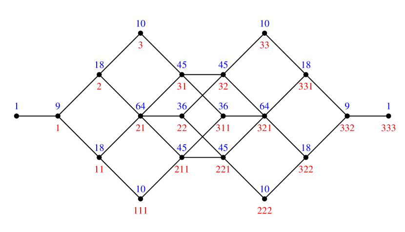
Figure 1. The ideal poset for $\operatorname{Gr}(3,6)$. The lower label on each node is the $\mathsf{a}\in{\mathsf{P}}(3,6)$ associated to the node and the upper label is the dimension of the corresponding subspace of $\Lambda^{*,0}(\operatorname{\mathfrak{m}})$.

3. Extremal Cycles in Grassmannians

3.1. Ideals of degree $2$

In this section, I am going to analyze the integral varieties of ${\mathcal{I}}_{(2)}$ and ${\mathcal{I}}_{(1,1)}$. The main application will be to giving a complete description of the the effective cycles of dimension $2$ or more whose homology classes are either of the form $r[\sigma_{(1,\dots,1)^{*}}]$ (see Theorem 2) or $r[\sigma_{(p)^{*}}]$ (see Theorem 5). Essentially, these results state that such cycles are represented only by subvarieties of projective spaces ‘in disguise’.

3.1.1. Integrals of ${\mathcal{I}}_{(2)}$

First, a characterization of the irreducible integral varieties of ${\mathcal{I}}_{(2)}$.

Proposition 3.

For every $A\in\operatorname{Gr}(m{+}1,n)$, the submanifold $\operatorname{Gr}(m,A)\subset\operatorname{Gr}(m,n)$ is an integral manifold of ${\mathcal{I}}_{(2)}$.

Conversely if $X\subset\operatorname{Gr}(m,n)$ is an integral variety of ${\mathcal{I}}_{(2)}$ that is irreducible and of dimension $d\geq 2$, then $X\subset\operatorname{Gr}(m,A)$ for some unique $A\in\operatorname{Gr}(m{+}1,n)$.

Proof.

It is immediate that, for any $A\in\operatorname{Gr}(m{+}1,n)$, the submanifold $\operatorname{Gr}(m,A)$ is an integral manifold of ${\mathcal{I}}_{(2)}$.

Suppose that $X\subset\operatorname{Gr}(m,n)$ satisfies the stated hypotheses and let $X^{\circ}\subset X$ denote the smooth part of $X$, which is connected since $X$ is irreducible [11, p. 21]. By hypothesis,  $X^{\circ}$ is an integral manifold of ${\mathcal{I}}_{(2)}$, i.e., its tangent planes are integral elements of ${\mathcal{I}}_{(2)}$.

Since $d\geq 2$, Lemma 4 implies that for every $V\in X^{\circ}$ there is a $d$-plane $P_{V}\subset V^{*}$ and a line $L_{V}\subset Q_{V}=\mathbb{C}^{\,n}/V$ so that

(3.1) $$T_{V}X=L_{V}\otimes P_{V}\subset Q_{V}\otimes V^{*}=T_{V}\operatorname{Gr}(m,n).$$

Now consider the set $F\subset X^{\circ}\times\operatorname{SL}(n,{\mathbb{C}})$ consisting of the set of pairs $(V,\mathsf{v})$ so that $V\in X^{\circ}$ and

1. $\mathsf{v}_{1},\dots,\mathsf{v}_{m}$ spans $V$;

2. $\mathsf{v}_{1},\dots,\mathsf{v}_{m-d}$ spans the annihilator of $P_{V}$; and

3. $[\![\mathsf{v}_{m+1}]\!]$ spans $L_{V}\subset Q_{V}$.

Then $F$ is a holomorphic $G$-bundle over $X^{\circ}$ where $G\subset\operatorname{SL}(n,{\mathbb{C}})$ is the parabolic subgroup that stabilizes $\mathbb{C}^{\,m-d}$, $\mathbb{C}^{\,m}$, and $\mathbb{C}^{\,m+1}$, i.e.,

$$G=P_{m-d}\cap P_{m}\cap P_{m+1}.$$

From now on, all computations will take place on $F$ or subbundles of $F$. Since  $X^{\circ}$ and $G$ are connected, $F$ is connected as well.

Consider the structure equations

(3.2) $$\mathrm{d}\mathsf{v}_{A}=\mathsf{v}_{B}\,\omega^{B}_{A}\,,\qquad\qquad\mathrm{d}\omega^{A}_{B}=-\omega^{A}_{C}{\mathchoice{\,{\scriptstyle\wedge}\,}{{\scriptstyle\wedge}}{{\scriptscriptstyle\wedge}}{{\scriptscriptstyle\wedge}}}\omega^{C}_{B}\,.$$

By (3.1) and the definition of $F$, it follows that $\omega^{\alpha}_{i}=0$ for all pairs $(i,\alpha)$ satisfying either $1\leq i\leq m{-}d$ and $\alpha=m{+}1$ or $1\leq i\leq m$ and $m{+}1<\alpha\leq n$. On the other hand, $\omega^{m+1}_{m-d+1}{\mathchoice{\,{\scriptstyle\wedge}\,}{{\scriptstyle\wedge}}{{\scriptscriptstyle\wedge}}{{\scriptscriptstyle\wedge}}}\dots\mathchoice{\,{\scriptstyle\wedge}\,}{{\scriptstyle\wedge}}{{\scriptscriptstyle\wedge}}{{\scriptscriptstyle\wedge}}\omega^{m+1}_{m}\not=0$.

Consequently, taking $\alpha>m{+}1$ and $j$ satisfying  $m{-}d<j\leq m$ and computing exterior derivatives via the structure equations yields

(3.3) $$0=\mathrm{d}\omega^{\alpha}_{j}=-\omega^{\alpha}_{A}{\mathchoice{\,{\scriptstyle\wedge}\,}{{\scriptstyle\wedge}}{{\scriptscriptstyle\wedge}}{{\scriptscriptstyle\wedge}}}\omega^{A}_{j}=-\omega^{\alpha}_{m+1}{\mathchoice{\,{\scriptstyle\wedge}\,}{{\scriptstyle\wedge}}{{\scriptscriptstyle\wedge}}{{\scriptscriptstyle\wedge}}}\omega^{m+1}_{j}\,.$$

Since $\omega^{m+1}_{m-d+1}{\mathchoice{\,{\scriptstyle\wedge}\,}{{\scriptstyle\wedge}}{{\scriptscriptstyle\wedge}}{{\scriptscriptstyle\wedge}}}\dots\mathchoice{\,{\scriptstyle\wedge}\,}{{\scriptstyle\wedge}}{{\scriptscriptstyle\wedge}}{{\scriptscriptstyle\wedge}}\omega^{m+1}_{m}\not=0$ and $d\geq 2$, this implies $\omega^{\alpha}_{m+1}=0$ when $\alpha>m{+}1$.

Since $\omega^{\alpha}_{i}=0$ for all pairs $(i,\alpha)$ satisfying $1\leq i\leq m{+}1<\alpha\leq n$, it follows that

(3.4) $$\mathrm{d}\mathsf{v}_{1}\equiv\dots\equiv\mathrm{d}\mathsf{v}_{m+1}\equiv 0\mod\mathsf{v}_{1},\dots,\mathsf{v}_{m+1}\,.$$

Thus, the span of the $\mathbb{C}^{\,n}$-valued functions $\mathsf{v}_{1},\dots,\mathsf{v}_{m+1}$ is locally constant on $F$. Since $F$ is connected, this span is constant. Let $A\subset\mathbb{C}^{\,n}$ be this span. By construction $A$ contains $V$ for all $V\in X^{\circ}$. Thus, $X^{\circ}$ lies in $\operatorname{Gr}(m,A)$. Since $X^{\circ}$ is dense in $X$, it follows that $X$ itself lies in $\operatorname{Gr}(m,A)\simeq{\mathbb{P}}(A^{*})$, as claimed. ∎

Proposition 3 has some interesting consequences.

Theorem 2.

Suppose that $1<p\leq m$ and let $\mathsf{a}=(1,\dots,1)$ with $|\mathsf{a}|=p$. Let $X\subset\operatorname{Gr}(m,n)$ be an irreducible $p$-dimensional variety that satisfies $[X]=r\,[\sigma_{\mathsf{a}^{*}}]$ for some $r\in{\mathbb{Z}}^{+}$. Then there exists a unique $A\in\operatorname{Gr}(m{+}1,n)$ so that

$$X\subset\operatorname{Gr}(m,A)\quad\left(\simeq{\mathbb{P}}(A^{*})\simeq{\mathbb{P}}^{m}\right)$$

and $r$ is the degree of $X$ as a variety in ${\mathbb{P}}^{m}$.

Conversely, for $A\in\operatorname{Gr}(m{+}1,n)$, any subvariety $X\subset\operatorname{Gr}(m,A)\subset\operatorname{Gr}(m,n)$ of dimension $p$ and degree $r$ satisfies $[X]=r\,[\sigma_{\mathsf{a}^{*}}]$.

Proof.

Since $[X]=r\,[\sigma_{\mathsf{a}^{*}}]$, it follows that $\phi_{\mathsf{b}}$ vanishes on $X^{\circ}$, the smooth part of $X$, for all $\mathsf{b}\in{\mathsf{P}}(m,n)$ with $|\mathsf{b}|=p$ and $\mathsf{b}\not=\mathsf{a}$. Consider the positive $(p,p)$-form $(\phi_{1})^{p-2}{\mathchoice{\,{\scriptstyle\wedge}\,}{{\scriptstyle\wedge}}{{\scriptscriptstyle\wedge}}{{\scriptscriptstyle\wedge}}}\phi_{2}$. (This is where the hypothesis $p>1$ is used.) By Pieri’s formula (2.30)

$$(\phi_{1})^{p-2}{\mathchoice{\,{\scriptstyle\wedge}\,}{{\scriptstyle\wedge}}{{\scriptscriptstyle\wedge}}{{\scriptscriptstyle\wedge}}}\phi_{(2)}=\sum_{\begin{subarray}{c}\mathsf{b}\in{\mathsf{P}}(m,n)\\ |\mathsf{b}|=p\end{subarray}}\mu^{\mathsf{b}}_{(2)}\,\phi_{\mathsf{b}}\,.$$

Since $\mathsf{a}\not\geq(2)$, it follows that $\mu^{\mathsf{a}}_{(2)}=0$, so every term on the right hand side of the above equation vanishes on $X^{\circ}$. Thus $(\phi_{1})^{p-2}{\mathchoice{\,{\scriptstyle\wedge}\,}{{\scriptstyle\wedge}}{{\scriptscriptstyle\wedge}}{{\scriptscriptstyle\wedge}}}\phi_{2}$ vanishes on $X^{\circ}$ as well. Since $\phi_{1}$ defines a Kähler form on $X^{\circ}$, the generalized Wirtinger inequality (1.18) implies that $\phi_{2}$ must vanish on $X^{\circ}$. In particular, $X$ is an integral manifold of ${\mathcal{I}}_{(2)}$. Since $X$ is irreducible and of dimension $p>1$, Proposition 3 applies. The statements about degree now follow immediately. ∎

This result has an interesting consequence of its own:

Theorem 3.

Suppose that $m>1$ and let $\mathsf{a}=(1,\dots,1)$, where $|\mathsf{a}|=m$. Let $X\subset\operatorname{Gr}(m,n)$ be an irreducible $m$-dimensional variety that satisfies $[X]=r\,[\sigma_{\mathsf{a}^{*}}]$ for some $r\in{\mathbb{Z}}^{+}$. Then $r=1$ and there exists a unique $A\in\operatorname{Gr}(m{+}1,n)$ so that $X=\operatorname{Gr}(m,A)$. (In particular, $X$ is a Schubert variety $\sigma_{\mathsf{a}^{*}}$.)

Remark 24 (Walters’ results).

When $m=2$, Theorem 3 was proved by Walters [27, Theorem 5 and Corollary 3]. Her proof relies on a local computation in coordinates that, essentially, computes the $2$-dimensional integral elements of ${\mathcal{I}}_{(2)}$ in the case $m=2$ (see [27, Claim 4.2.3]) and then, using this, proves a coordinate version of Proposition 3 in this case.

Remark 25 (Schur rigidity and quasi-rigidity).

As was mentioned already in §2.8.3, Walters showed that $\mathsf{a}=((m)^{\prime})^{*}$, has Schubert rigidity, i.e., that any (local) solution of $\mathcal{B}_{\mathsf{a}}$ is a Schubert variety $\sigma_{\mathsf{a}}$. Theorem 3 shows that this $\mathsf{a}$ even has Schur rigidity. This is not surprising, though, because, as the proof of Theorem 2 makes clear, $\mathcal{B}_{\mathsf{a}}=\mathcal{R}_{\mathsf{a}^{*}}$ for all $\mathsf{a}$ of the form $((p)^{\prime})^{*}$ when $p>1$.

Walters also showed that, when $p<m$, the type $\mathsf{a}=((p)^{\prime})^{*}$ does not have Schubert rigidity. However, she did not classify the solutions to $\mathcal{B}_{\mathsf{a}}$ in this case. Theorem 2 does this classification in the range $1<p<m$, showing that such an irreducible variety is a $p$-dimensional subvariety of a projective space $\operatorname{Gr}(m,A)\simeq{\mathbb{P}}^{m}$ for some $A\in\operatorname{Gr}(m{+}1,n)$.

Since $\mathcal{B}_{(1)^{*}}\not=\mathcal{R}_{(1)}$, the solutions of $\mathcal{B}_{(1)^{*}}$ (the omitted case) are of a different nature. However, it is not difficult to show that an irreducible curve in $\operatorname{Gr}(m,n)$ that is a solution of $\mathcal{B}_{(1)^{*}}$ can be described as follows: Fix a subspace $W\subset\mathbb{C}^{\,n}$ of dimension $k<m$ and let $C\subset{\mathbb{P}}\bigl{(}\mathbb{C}^{\,n}/W\bigr{)}\simeq{\mathbb{P}}^{n-k-1}$ be a projective curve that spans a projective subspace of dimension at least $m{-}k$. Let $C^{[m-k-1]}\subset\operatorname{Gr}\bigl{(}m{-}k,\mathbb{C}^{\,n}/W\bigr{)}$ be the $(m{-}k{-}1)$-th osculating curve of $C$ and consider its inclusion into $\operatorname{Gr}(m,n)$ by the canonical injection $\operatorname{Gr}\bigl{(}m{-}k,\mathbb{C}^{\,n}/W\bigr{)}\hookrightarrow\operatorname{Gr}(m,n).$ This image curve is a solution to $\mathcal{B}_{(1)^{*}}$ and every irreducible solution is of this form.

3.1.2. Bundles with $c_{2}=0$

Proposition 3 can also be applied to characterize bundles generated by their sections but with vanishing second Chern class.

Theorem 4.

Let $M$ be a connected compact Kähler manifold and let $F\to M$ be a holomorphic vector bundle that is generated by its sections. If $c_{2}(F)=0$, then either there exists a holomorphic splitting $F=L\oplus T$ where $L$ is a line bundle and $T$ is trivial or else there exists an algebraic curve $C$, a bundle $F^{\prime}\to C$ that is generated by its sections, and a holomorphic mapping $\kappa:M\to C$ so that $F=\kappa^{*}(F^{\prime})$.

Proof.

Since $F$ is generated by its sections, there exists an $n>0$ and a surjective holomorphic bundle map $\phi:M\times\mathbb{C}^{\,n}\to F$. Let $m\leq n$ be the rank of the kernel bundle $K\subset M\times\mathbb{C}^{\,n}$. The mapping $\kappa:M\to\operatorname{Gr}(m,n)$ defined by $\kappa(x)=K_{x}$ then has the property that $F=\kappa^{*}(Q)$. Moreover, $c_{2}(F)=\kappa^{*}\bigl{(}c_{2}(Q)\bigr{)}=\kappa^{*}(q_{2})$.

Since $[\phi_{2}]=c_{2}(Q)=q_{2}$ and $\phi_{2}$ is a positive $(2,2)$-form, it follows that $\kappa^{*}(\phi_{2})$ is a positive $(2,2)$-form on $M$ that represents $c_{2}(F)$. Since $M$ is compact and Kähler, the hypothesis $c_{2}(F)=0$ implies that the representing positive form $\kappa^{*}(\phi_{2})$ must also be zero by Corollary 1. Equivalently, $\kappa(M)\subset\operatorname{Gr}(m,n)$ is an integral variety of ${\mathcal{I}}_{(2)}$. Since $M$ is connected, $\kappa(M)$ is irreducible. Now there are three cases:

If the dimension of $\kappa(M)$ is equal to $0$, then $\kappa$ is constant and $F=\kappa^{*}(Q)$ is trivial. This falls into both of the two cases allowed by the proposition.

If the dimension of $\kappa(M)$ is equal to $1$, then $\kappa(M)$ is an algebraic curve $C\subset\operatorname{Gr}(m,n)$. Replace $C$ by its normalization if necessary and define $F^{\prime}\to C$ to be the pullback to $C$ of the bundle $Q\to\operatorname{Gr}(m,n)$. Then $\kappa^{*}(F^{\prime})=F$.

If the dimension of $\kappa(M)$ is greater than $1$, then Proposition 3 implies that there exists an $(m{+}1)$-plane $A\subset\mathbb{C}^{\,n}$ so that $\kappa(M)\subset\operatorname{Gr}(m,A)$. Let $B\subset\mathbb{C}^{\,n}$ be a subspace of dimension $n{-}m{-}1$ that is a complement to $A$. The bundle $Q$ restricted to $\operatorname{Gr}(m,A)$ splits as a sum $L^{\prime}\oplus T^{\prime}$ where $L^{\prime}$ is a line bundle and $T^{\prime}$ is trivial. Explicitly, for $V\in\operatorname{Gr}(m,A)$, $L^{\prime}_{V}=A/V$ and $T^{\prime}_{V}=B$. Setting $L=\kappa^{*}(L^{\prime})$ and $T=\kappa^{*}(T^{\prime})$ yields the desired splitting. ∎

3.1.3. Integrals of ${\mathcal{I}}_{(1,1)}$

Now, all of these results from the analysis of ${\mathcal{I}}_{(2)}$ can be translated by complementarity into corresponding results from the analysis of ${\mathcal{I}}_{(1,1)}$:

Proposition 4.

Suppose that $n{-}m\geq 2$ and let $V\subset\operatorname{Gr}(m,n)$ be an irreducible subvariety of dimension $d>1$ that is an integral manifold of ${\mathcal{I}}_{(1,1)}$. Then there is a unique $A\in\operatorname{Gr}(m{-}1,n)$ so that

$$V\subset[A,\mathbb{C}^{\,n}]_{m}\quad\left(\ =\operatorname{Gr}(1,\mathbb{C}^{\,n}/A)\simeq{\mathbb{P}}^{n-m}\right).$$

Conversely, for every $A\in\operatorname{Gr}(m{-}1,n)$, the submanifold $[A,\mathbb{C}^{\,n}]_{m}\subset\operatorname{Gr}(m,n)$ is an integral manifold of ${\mathcal{I}}_{(1,1)}$.

Proof.

Apply complementarity to the proof of Proposition 3. ∎

This proposition can be applied to characterize the cycles representing a number of extremal classes.

Theorem 5.

Suppose that $1<p\leq n{-}m$ and let $V\subset\operatorname{Gr}(m,n)$ be an irreducible $p$-dimensional variety that satisfies $[V]=r\,[\sigma_{(p)^{*}}]$ for some $r\in{\mathbb{Z}}^{+}$. Then there exists a unique $A\in\operatorname{Gr}(m{-}1,n)$ so that

$$V\subset[A,\mathbb{C}^{\,n}]_{m}\quad\left(\simeq{\mathbb{P}}(\mathbb{C}^{\,n}/A)\simeq{\mathbb{P}}^{n-m}\right)$$

and $r$ is the degree of $V$ as a variety in ${\mathbb{P}}^{n-m}$. Conversely, for each $A\in\operatorname{Gr}(m{-}1,n)$, any $p$-dimensional variety $V\subset[A,\mathbb{C}^{\,n}]_{m}$ of degree $r$ satisfies $[V]=r\,[\sigma_{(p)^{*}}]$.

Proof.

Apply complementarity to the proof of Theorem 2. ∎

Remark 26 (Walters’ results).

These results when $p=2$ and $m=2$ are also (partially) to be found in the work of Walters.

Remark 27 (Another Schur-Schubert coincidence).

Note that Theorem 5 also implies that $\mathcal{B}_{\mathsf{a}}=\mathcal{R}_{\mathsf{a}^{*}}$ when $\mathsf{a}=(p)^{*}$ for $p>1$. However, this could have been proved directly, using the algebraic ideas that went into the proof.

3.1.4. Bundles with ${c_{1}}^{2}-c_{2}=0$

Proposition 4 can also be applied to characterize bundles generated by their sections but with vanishing Schur-Chern polynomial $c_{(1,1)}$.

Theorem 6.

Let $M$ be a connected compact Kähler manifold and let $F\to M$ be a holomorphic vector bundle of rank $r$ that is generated by its sections.

Then $c_{1}(F)^{2}-c_{2}(F)\geq 0$ and, if equality holds, either $F=(M{\times}\mathbb{C}^{\,r+1})/L$ for some line bundle $L\subset M{\times}\mathbb{C}^{\,r+1}$ or else there exists an algebraic curve $C$, a bundle $F^{\prime}\to C$ that is generated by its sections, and a holomorphic mapping $\kappa:M\to C$ so that $F=\kappa^{*}(F^{\prime})$.

Proof.

Let $H^{0}(F)$ be the space of global sections of $F$, a vector space of dimension $n=h^{0}(F)$. Let $\operatorname{ev}_{\!F}:M\times H^{0}(F)\to F$ be the evaluation mapping, which, by assumption, is surjective, so that $n\geq r$. The kernel $K\subset M\times H^{0}(F)$ is then a subbundle of rank $m=n{-}r$ and can be used to define a mapping $\kappa_{F}:M\to\operatorname{Gr}\bigl{(}m,H^{0}(F)\bigr{)}$ that satisfies  $\kappa_{F}^{*}(Q)=F$. Consequently,

$$c_{1}(F)^{2}-c_{2}(F)=c_{(1,1)}(F)=\left[\kappa^{*}(\phi_{(1,1)})\right].$$

Thus, the inequality $c_{1}(F)^{2}-c_{2}(F)\geq 0$ follows directly from Corollary 1. Moreover, if equality holds, $\kappa_{F}(M)\subset\operatorname{Gr}\bigl{(}m,H^{0}(F)\bigr{)}$ must be an integral variety of ${\mathcal{I}}_{(1,1)}$. As in the proof of Theorem 4, there are now three cases:

If $\kappa_{F}(M)$ is a single point, then $F$ is trivial.

If $\kappa_{F}(M)$ is a curve, let $C\to\kappa_{F}(M)\subset\operatorname{Gr}\bigl{(}m,H^{0}(F)\bigr{)}$ be its normalization and let $F^{\prime}$ be the pullback of $Q$ to $C$.

If $\kappa_{F}(M)$ has dimension greater than $1$, then Proposition 4 implies that there is an $(m{-}1)$-plane $A\subset H^{0}(F)$ so that $\kappa_{F}(M)\subset\bigl{[}A,H^{0}(F)\bigr{]}_{m}$. However, this implies that $M\times A$ is a subset of $K$. In other words, $A$ consists of the global sections of $F$ that vanish at all points of $M$. Of course, this implies that $A=(0)$, i.e., that $m=1$, so that $H^{0}(F)=n=r{+}m=r{+}1$, which is what needed to be shown. ∎

3.2. Ideals of codegree $2$

In this subsection, I will analyze the maximal dimension integral varieties of the ideals ${\mathcal{I}}_{(1,1)^{*}}$ and ${\mathcal{I}}_{(2)^{*}}$, namely their integral varieties of codimension $2$ in $\operatorname{Gr}(m,n)$. This is not really of interest unless both ideals are nontrivial, so I will assume that $2\leq m\leq n{-}2$. In this case, $[\sigma_{(2)}]$ and $[\sigma_{(1,1)}]$ are linearly independent and give a basis of $H_{m(n-m)-4}\bigl{(}\operatorname{Gr}(m,n),{\mathbb{Z}}\bigr{)}$. The goal of this subsection is to give a description of the effective cycles representing these classes, so I state the main results in those terms, rather than directly in terms of the integral varieties of the ideals.

One reason for interest in these results is that the comparison of the nonsmoothability of these varieties with the nonsmoothability results of Hartshorne, Rees, and Thomas [14].

3.2.1. Integrals of ${\mathcal{I}}_{(1,1)^{*}}$

Consider the class $[\sigma_{(2)}]$. Recall that $\sigma_{(2)}\subset\operatorname{Gr}(m,n)$ consists of the $m$-planes $E\subset\mathbb{C}^{\,n}$ that meet $\mathbb{C}^{\,n-m-1}$ in at least a line. Equivalently, this is the same as requiring that ${\mathbb{P}}E\subset{\mathbb{P}}^{n-1}$ meet a fixed ${\mathbb{P}}^{n-m-2}\subset{\mathbb{P}}^{n-1}$.

Theorem 7.

For any algebraic variety $A\subset\operatorname{Gr}(1,n)$ of codimension $m{+}1$ and degree $r$, the variety

$$\Psi_{m}(A)=\bigl{\{}\,E\in\operatorname{Gr}(m,n)\mid{\mathbb{P}}E\cap A\not=\emptyset\,\}$$

is of codimension $2$ in $\operatorname{Gr}(m,n)$ and satisfies $\bigl{[}\Psi_{m}(A)\bigr{]}=r\,[\sigma_{(2)}]$.

Conversely, if $V\subset\operatorname{Gr}(m,n)$ is an algebraic variety of codimension $2$ that satisfies $[V]=r\,[\sigma_{(2)}]$ for some $r\in{\mathbb{Z}}^{+}$, then $V=\Psi_{m}(A)$ for some unique algebraic variety $A\subset\operatorname{Gr}(1,n)$ of codimension $m{+}1$ and degree $r$.

Proof.

Let $A\subset\operatorname{Gr}(1,n)\simeq{\mathbb{P}}^{n-1}$ be an algebraic variety of codimension $m{+}1$ and degree $r$. It is immediate that $\Psi_{m}(A)$ is of codimension $2$. Moreover, a simple local calculation shows that, at its smooth points, its tangent spaces are integral elements of ${\mathcal{I}}_{(1,1)^{*}}$ (cf. Corollary 7). Thus, $\phi_{(1,1)^{*}}$ vanishes on $\Psi_{m}(A)$, which implies that $\bigl{[}\Psi_{m}(A)\bigr{]}=r^{\prime}\,[\sigma_{(2)}]$ for some $r^{\prime}$. Since $r^{\prime}=1$ when $r=1$, it follows easily that $r^{\prime}=r$ in all cases.

Now, for the converse statement, it clearly suffices to prove the characterization when $V$ is irreducible, so assume this. Thus suppose that $V\subset\operatorname{Gr}(m,n)$ satisfies the stated hypotheses and is irreducible. Let $V^{\circ}\subset V$ denote the smooth part of $V$, which is connected, since $V$ is irreducible. Since $[V]=r\,[\sigma_{(2)}]$, this smooth part $V^{\circ}$ must be an integral manifold of ${\mathcal{I}}_{(1,1)^{*}}$, i.e., its tangent planes must be integral elements of ${\mathcal{I}}_{(1,1)^{*}}$. Thus, by Lemma 7, for every $E\in V^{\circ}$ there exists a line $L_{E}\subset E$ and a codimension $2$ subspace $R_{E}\subset Q_{E}=\mathbb{C}^{\,n}/E$ so that

(3.5) $$T_{E}V=\bigl{(}R_{E}{\otimes}E^{*}\bigr{)}+\bigl{(}Q_{E}{\otimes}L_{E}^{\perp}\bigr{)}\subset Q_{E}\otimes E^{*}=T_{E}\operatorname{Gr}(m,n).$$

Consider the set $F\subset V^{\circ}\times\operatorname{GL}(n,{\mathbb{C}})$ consisting of the set of pairs $(E,\mathsf{v})$ so that

1. $\mathsf{v}_{1}$ spans $L_{E}$;

2. $\mathsf{v}_{1},\dots,\mathsf{v}_{m}$ spans $E$; and

3. $[\![\mathsf{v}_{m+1}]\!]_{E},\dots,[\![\mathsf{v}_{n-2}]\!]_{E}$ spans $R_{E}\subset Q_{E}$.

Then $F$ is a holomorphic $G$-bundle over $V^{\circ}$ where $G\subset\operatorname{GL}(n,{\mathbb{C}})$ is the parabolic subgroup that stabilizes $\mathbb{C}^{\,1}$, $\mathbb{C}^{\,m}$, and $\mathbb{C}^{\,n-2}$. From now on, all computations will take place on $F$ or subbundles of $F$. Of course, since $G$ is connected and since $V^{\circ}$ is connected, it follows that $F$ is connected as well.

Consider the structure equations

(3.6) $$\begin{split}\mathrm{d}\mathsf{v}_{A}&=\mathsf{v}_{B}\,\omega^{B}_{A}\,,\\ \mathrm{d}\omega^{A}_{B}&=-\omega^{A}_{C}{\mathchoice{\,{\scriptstyle\wedge}\,}{{\scriptstyle\wedge}}{{\scriptscriptstyle\wedge}}{{\scriptscriptstyle\wedge}}}\omega^{C}_{B}\,.\\ \end{split}$$

By (3.5) and the definition of $F$, it follows that $\omega^{n-1}_{1}=\omega^{n}_{1}=0$ and, moreover, that these two relations are the only linear relations among the $m(n{-}m)$ forms $\omega^{a}_{i}$ with $1\leq i\leq m<a\leq n$. Note that these latter forms generate the module of forms that are semibasic for the fibration $\pi:F\to V^{\circ}$.

Computing exterior derivatives via the structure equations yields

(3.7) $$\begin{split}0=\mathrm{d}\omega^{n-1}_{1}&={}-\omega^{n-1}_{A}{\mathchoice{\,{\scriptstyle\wedge}\,}{{\scriptstyle\wedge}}{{\scriptscriptstyle\wedge}}{{\scriptscriptstyle\wedge}}}\omega^{A}_{1}=-\sum_{j=2}^{m}\omega^{n-1}_{j}{\mathchoice{\,{\scriptstyle\wedge}\,}{{\scriptstyle\wedge}}{{\scriptscriptstyle\wedge}}{{\scriptscriptstyle\wedge}}}\omega^{j}_{1}-\sum_{a=m+1}^{n-2}\omega^{n-1}_{a}{\mathchoice{\,{\scriptstyle\wedge}\,}{{\scriptstyle\wedge}}{{\scriptscriptstyle\wedge}}{{\scriptscriptstyle\wedge}}}\omega^{a}_{1}\,,\\ 0=\mathrm{d}\omega^{n\phantom{-1}}_{1}&={}-\omega^{n\phantom{-1}}_{A}{\mathchoice{\,{\scriptstyle\wedge}\,}{{\scriptstyle\wedge}}{{\scriptscriptstyle\wedge}}{{\scriptscriptstyle\wedge}}}\omega^{A}_{1}=-\sum_{j=2}^{m}\omega^{n\phantom{-1}}_{j}{\mathchoice{\,{\scriptstyle\wedge}\,}{{\scriptstyle\wedge}}{{\scriptscriptstyle\wedge}}{{\scriptscriptstyle\wedge}}}\omega^{j}_{1}-\sum_{a=m+1}^{n}\omega^{n\phantom{-1}}_{a}{\mathchoice{\,{\scriptstyle\wedge}\,}{{\scriptstyle\wedge}}{{\scriptscriptstyle\wedge}}{{\scriptscriptstyle\wedge}}}\omega^{a}_{1}\,.\\ \end{split}$$

Reducing these equations modulo $\{\omega^{m+1}_{1},\ldots,\omega^{n-2}_{1}\}$ yields

(3.8) $$\sum_{j=2}^{m}\omega^{n-1}_{j}{\mathchoice{\,{\scriptstyle\wedge}\,}{{\scriptstyle\wedge}}{{\scriptscriptstyle\wedge}}{{\scriptscriptstyle\wedge}}}\omega^{j}_{1}\equiv\sum_{j=2}^{m}\omega^{n}_{j}{\mathchoice{\,{\scriptstyle\wedge}\,}{{\scriptstyle\wedge}}{{\scriptscriptstyle\wedge}}{{\scriptscriptstyle\wedge}}}\omega^{j}_{1}\equiv 0\mod\omega^{m+1}_{1},\ldots,\omega^{n-2}_{1}\,.$$

Since $\{\omega^{n-1}_{j},\omega^{n}_{j}\mid 2\leq j\leq m\}$ are linearly independent modulo $\{\omega^{m+1}_{1},\ldots,\omega^{n-2}_{1}\}$, these equations imply that

(3.9) $$\omega^{2}_{1}\equiv\dots\equiv\omega^{k}_{1}\equiv 0\mod\omega^{m+1}_{1},\ldots,\omega^{n-2}_{1}\,.$$

Thus, there exist functions $\{\,s^{j}_{a}\mid 2\leq j\leq m<a\leq n{-}2\,\}$ on $F$ so that $\omega^{j}_{1}=s^{j}_{a}\,\omega^{a}_{1}$. The structure equations now imply that

(3.10) $$d\mathsf{v}_{1}\equiv\sum_{a=m+1}^{n-2}(\mathsf{v}_{a}+s^{j}_{a}\,\mathsf{v}_{j})\,\omega^{a}_{1}\mod\mathsf{v}_{1}\,.$$

Consequently, the map $[\mathsf{v}_{1}]:F\to\operatorname{Gr}(1,\mathbb{C}^{\,n})={\mathbb{P}}^{n-1}$ is a holomorphic map of constant rank $n{-}m{-}2$. Moreover, since the forms $\{\omega^{m+1}_{1},\ldots,\omega^{n-2}_{1}\}$ are $\pi$-semibasic, and $\pi$ has connected fibers, it follows that there is a well-defined holomorphic map $\lambda:V^{\circ}\to{\mathbb{P}}^{n-1}$ of constant rank $n{-}m{-}2$ that satisfies $\lambda(E)=L_{E}$, i.e., $[\mathsf{v}_{1}]=\lambda\circ\pi$.

By dimension count, the fibers of $\lambda$ have dimension $m(n{-}m){-}2-(n{-}m{-}2)=(m{-}1)(n{-}m)$. Moreover, by construction, for each line $L=\lambda(E)$, the fiber $\lambda^{-1}(L)$ is embedded as a submanifold of the sub-Grassmannian $[L,\mathbb{C}^{\,n}]_{m}\subset\operatorname{Gr}(m,n)$, which also has dimension $(m{-}1)(n{-}m)$. It follows that $V^{\circ}\cap[L,\mathbb{C}^{\,n}]_{m}$ is an open subset of $[L,\mathbb{C}^{\,n}]_{m}$. Since $V$ is algebraic, it follows that $V$ must actually contain $[L,\mathbb{C}^{\,n}]_{m}$ for all $L\in\lambda(V^{\circ})$.

Let $B\subset~{}\operatorname{Gr}(1,\mathbb{C}^{\,n})$ be the set of lines $L$ for which $[L,\mathbb{C}^{\,n}]_{m}$ lies in $V$. Then $B$ is evidently a variety that has at least one component $B^{\prime}$ of dimension $d\geq n{-}m{-}2$. Since, in particular, $V$ must contain all of the $m$-planes that meet $B^{\prime}$, it follows that the dimension of $B^{\prime}$ cannot be more than $n{-}m{-}2$ (otherwise, it would impose at most one condition for a ${\mathbb{P}}^{m-1}\subset{\mathbb{P}}^{n-1}$ to meet $B^{\prime}$). By connectedness, the image $\lambda(V^{\circ})$ must lie in a component of $B$, say $A\subset B$ that has the maximum possible dimension, namely $n{-}m{-}2$.

Let $W\subset V$ denote the set of $m$-planes $E$ satisfying ${\mathbb{P}}(E)\cap A\not=\emptyset$. Then, since $A$ has dimension $n{-}m{-}2$, it follows that $W$ has the same dimension as $V$. Since $V$ is irreducible, $W=V$. Now, if $B$ had any other component $A^{\prime}\not=A$ of dimension $n{-}m{-}2$, then the corresponding $W^{\prime}$ would also satisfy $W^{\prime}=V$ and, consequently, $W^{\prime}=W$. However, this would imply that every ${\mathbb{P}}^{m-1}$ that meets $A$ must also meet $A^{\prime}$ and vice versa. But if $A\not=A^{\prime}$, this is absurd. Thus, $A$ is unique.

Finally, the equation $r=\deg(A)$ and the converse follow by the Schubert calculus and calculation, respectively. ∎

Remark 28 (Integral varieties of ${\mathcal{I}}_{(1,1)^{*}}$).

The reader may have expected Theorem 7 to have been stated in terms of a characterization of the irreducible integral varieties of ${\mathcal{I}}_{(1,1)^{*}}$ of codimension $2$. There is, of course, such a characterization and it follows the more-or-less expected lines except for one caveat: What is true (and the above proof can be easily adapted so as to prove it) is that every codimension $2$, irreducible integral variety $V$ of ${\mathcal{I}}_{(1,1)^{*}}$ is locally of the form $\Psi_{m}(A)$ for some irreducible subvariety $A\subset\operatorname{Gr}(1,n)$ of dimension $n{-}m{-}2$. In this sense, the codimension $2$ integral manifolds of ${\mathcal{I}}_{(1,1)^{*}}$ depend (in Cartan’s sense) on $m{+}1$ functions of $n{-}m{-}2$ variables (in the holomorphic category). However, without some hypotheses on the ‘finiteness’ of the variety $V$, the mapping $\lambda:V^{\circ}\to\operatorname{Gr}(1,n)$ can be very far from proper, so that the image is not a variety, even locally. It is for this reason that I incorporated compactness into the statement of Theorem 7.

Example 15 (Rigidity of $\sigma_{(2)}$).

Theorem 7 shows that any $V\subset\operatorname{Gr}(m,n)$ of codimension $2$ that satisfies $[V]=[\sigma_{(2)}]$ must actually be a Schubert cycle, a very strong form of rigidity. Of course, when $(m,n)=(2,4)$, this result is classical [7] (and, in any case, already follows from the previous results on extremal subvarieties of dimension $2$).

Example 16 (Nonsmoothability).

Note that the variety $\Psi_{m}(A)\subset\operatorname{Gr}(m,n)$ will be singular as soon as $A$ is not a single point. Thus, Theorem 7 implies that if $n>m{+}2$, then any $V\subset\operatorname{Gr}(m,n)$ of codimension $2$ satisfying $[V]=r[\sigma_{(2)}]$ with $r>0$ must necessarily be singular.

In [14], the authors use results of Thom [26] to prove that, for any $r>0$, there are integers $m$ and $n$ for which the class $r[\sigma_{(2)}]$ in $H_{*}\bigl{(}\operatorname{Gr}(m,n),{\mathbb{Z}}\bigr{)}$ cannot be represented by a smooth manifold. While Thom’s results also show that, for every $m$ and $n>m{+}2$, there exists an $r>0$ for which $r[\sigma_{(2)}]$ is representable by a smooth manifold, Theorem 7 implies that, when $n>m{+}2$, the class $r[\sigma_{(2)}]$ is not representable by a smooth algebraic variety for any $r>0$.

If $n=m{+}2$, the cycle $\sigma_{(2)}=[\mathbb{C}^{\,1},\mathbb{C}^{\,m+2}]_{m}$ is isomorphic to $\operatorname{Gr}(m{-}1,m{+}1)$ and hence is smooth. Theorem 7 implies that if $V\subset\operatorname{Gr}(m,m{+}2)$ satisfies $[V]=r[\sigma_{(2)}]$, then

$$V=[L_{1},\mathbb{C}^{\,m+2}]_{m}\cup\dots\cup[L_{r},\mathbb{C}^{\,m+2}]_{m}$$

for some lines $L_{1},\dots,L_{r}\in\operatorname{Gr}(1,\mathbb{C}^{\,m+1})={\mathbb{P}}^{m+1}$. In particular, $V$ is singular when $r>1$.

3.2.2. Integrals of ${\mathcal{I}}_{(2)^{*}}$

Recall that $\sigma_{(1,1)}$ consists of the $m$-planes $E\subset\mathbb{C}^{\,n}$ that meet $\mathbb{C}^{\,n-m+1}$ in at least a $2$-plane. Now, $E$ satisfies this condition when $E+\mathbb{C}^{\,n-m+1}$ has dimension at most $n{-}1$, i.e., when $E$ lies in a hyperplane containing $\mathbb{C}^{\,n-m+1}$. Thus, another way of describing $\sigma_{(1,1)}$ is as the $m$-planes that lie in one of the hyperplanes in $\mathbb{C}^{\,n}$ that contain $\mathbb{C}^{\,n-m+1}$. The set of such hyperplanes forms a ${\mathbb{P}}^{m-2}$ in $\operatorname{Gr}(n{-}1,n)\simeq{\mathbb{P}}^{n-1}$. This description of $\sigma_{(1,1)}$ motivates the following result.

Theorem 8.

For any algebraic variety $A\subset\operatorname{Gr}(n{-}1,n)$ of dimension $m{-}2$ and degree $r$, the subvariety $V=\Sigma_{m}(A)$ defined by

$$\Sigma_{m}(A)=\cup_{H\in A}\operatorname{Gr}(m,H)$$

has codimension $2$ in $\operatorname{Gr}(m,n)$ and satisfies $[V]=r\,[\sigma_{(1,1)}]$.

Conversely, if $V\subset\operatorname{Gr}(m,n)$ is an algebraic variety of codimension $2$ that satisfies $[V]=r\,[\sigma_{(1,1)}]$ for some $r\in{\mathbb{Z}}^{+}$, then there exists a subvariety $A\subset\operatorname{Gr}(n{-}1,n)$ of dimension $m{-}2$ and degree $r$ so that $V=\Sigma_{m}(A)$.

Proof.

Let $A\subset\operatorname{Gr}(n{-}1,n)\simeq{\mathbb{P}}^{n-1}$ be an algebraic variety of dimension $m{-}2$ and degree $r$. A simple local calculation verifies that $\Sigma_{m}(A)$ as defined in the proposition has codimension $2$ in $\operatorname{Gr}(m,n)$ and that its tangent space at a smooth point is of type $(1,1)$. Consequently (cf. Corollary 6), it follows that $\bigl{[}\Sigma_{m}(A)\bigr{]}=r^{\prime}\bigl{[}\sigma_{(1,1)}\bigr{]}$ for some $r^{\prime}>0$. Since $r=1$ if and only if $A$ is a linear ${\mathbb{P}}^{m-2}$ and since, in this case, $\Sigma_{m}(A)$ is a Schubert cycle of type $(1,1)$, it follows that $r^{\prime}=1$ in this case. It now follows easily by a degree argument that $r^{\prime}=r$ in all cases.

Now, to prove, the converse, it clearly suffices to treat the case in which $V\subset\operatorname{Gr}(m,n)$ is irreducible, so assume this. Thus, suppose that $V\subset\operatorname{Gr}(m,n)$ satisfies the stated hypotheses and let $V^{\circ}\subset V$ denote the smooth part of $V$, which is connected, since $V$ is irreducible. Since $[V]=r\,[\sigma_{(1,1)}]$, this smooth part $V^{\circ}$ must be an integral manifold of ${\mathcal{I}}_{(2)^{*}}$, i.e., its tangent planes must be integral elements of ${\mathcal{I}}_{(2)^{*}}$. Thus, by Lemma 6, for every $E\in V^{\circ}$ there exists a 2-plane $P_{E}\subset E$ and a hyperplane $R_{E}\subset Q_{E}=\mathbb{C}^{\,n}/E$ so that

(3.11) $$T_{E}V=\bigl{(}R_{E}{\otimes}E^{*}\bigr{)}+\bigl{(}Q_{E}{\otimes}P_{E}^{\perp}\bigr{)}\subset Q_{E}\otimes E^{*}=T_{E}\operatorname{Gr}(m,n).$$

Consider the set $F\subset V^{\circ}\times\operatorname{GL}(n,{\mathbb{C}})$ consisting of the set of pairs $(E,\mathsf{v})$ so that

1. $\mathsf{v}_{1},\mathsf{v}_{2}$ spans $P_{E}$;

2. $\mathsf{v}_{1},\dots,\mathsf{v}_{m}$ spans $E$; and

3. $[\![\mathsf{v}_{m+1}]\!]_{E},\dots,[\![\mathsf{v}_{n-1}]\!]_{E}$ spans $R_{E}\subset Q_{E}$.

Then $F$ is a holomorphic $G$-bundle over $V^{\circ}$ where $G\subset\operatorname{GL}(n,{\mathbb{C}})$ is the parabolic subgroup that stabilizes $\mathbb{C}^{\,2}$, $\mathbb{C}^{\,m}$, and $\mathbb{C}^{\,n-1}$. From now on, all computations will take place on $F$ or subbundles of $F$. Of course, since $G$ is connected and since $V^{\circ}$ is connected, it follows that $F$ is connected as well.

Consider the structure equations

(3.12) $$\begin{split}\mathrm{d}\mathsf{v}_{A}&=\mathsf{v}_{B}\,\omega^{B}_{A}\,,\\ \mathrm{d}\omega^{A}_{B}&=-\omega^{A}_{C}{\mathchoice{\,{\scriptstyle\wedge}\,}{{\scriptstyle\wedge}}{{\scriptscriptstyle\wedge}}{{\scriptscriptstyle\wedge}}}\omega^{C}_{B}\,.\\ \end{split}$$

By (3.11) and the definition of $F$, it follows that $\omega^{n}_{1}=\omega^{n}_{2}=0$ and, moreover, that these two relations are the only linear relations among the $m(n{-}m)$ forms $\omega^{a}_{i}$ with $1\leq i\leq m<a\leq n$. Note that these latter forms generate the module of forms that are semibasic for the fibration $\pi:F\to V^{\circ}$.

Computing exterior derivatives via the structure equations yields

(3.13) $$\begin{split}0=\mathrm{d}\omega^{n}_{1}&={}-\omega^{n}_{A}{\mathchoice{\,{\scriptstyle\wedge}\,}{{\scriptstyle\wedge}}{{\scriptscriptstyle\wedge}}{{\scriptscriptstyle\wedge}}}\omega^{A}_{1}=-\sum_{j=3}^{m}\omega^{n}_{j}{\mathchoice{\,{\scriptstyle\wedge}\,}{{\scriptstyle\wedge}}{{\scriptscriptstyle\wedge}}{{\scriptscriptstyle\wedge}}}\omega^{j}_{1}-\sum_{a=m+1}^{n-1}\omega^{n}_{a}{\mathchoice{\,{\scriptstyle\wedge}\,}{{\scriptstyle\wedge}}{{\scriptscriptstyle\wedge}}{{\scriptscriptstyle\wedge}}}\omega^{a}_{1}\,,\\ 0=\mathrm{d}\omega^{n}_{2}&={}-\omega^{n}_{A}{\mathchoice{\,{\scriptstyle\wedge}\,}{{\scriptstyle\wedge}}{{\scriptscriptstyle\wedge}}{{\scriptscriptstyle\wedge}}}\omega^{A}_{2}=-\sum_{j=3}^{m}\omega^{n}_{j}{\mathchoice{\,{\scriptstyle\wedge}\,}{{\scriptstyle\wedge}}{{\scriptscriptstyle\wedge}}{{\scriptscriptstyle\wedge}}}\omega^{j}_{2}-\sum_{a=m+1}^{n-1}\omega^{n}_{a}{\mathchoice{\,{\scriptstyle\wedge}\,}{{\scriptstyle\wedge}}{{\scriptscriptstyle\wedge}}{{\scriptscriptstyle\wedge}}}\omega^{a}_{2}\,.\\ \end{split}$$

Reducing these equations modulo $\{\omega^{n}_{3},\ldots,\omega^{n}_{m}\}$ yields

(3.14) $$\sum_{a=m+1}^{n-1}\omega^{n}_{a}{\mathchoice{\,{\scriptstyle\wedge}\,}{{\scriptstyle\wedge}}{{\scriptscriptstyle\wedge}}{{\scriptscriptstyle\wedge}}}\omega^{a}_{1}\equiv\sum_{a=m+1}^{n-1}\omega^{n}_{a}{\mathchoice{\,{\scriptstyle\wedge}\,}{{\scriptstyle\wedge}}{{\scriptscriptstyle\wedge}}{{\scriptscriptstyle\wedge}}}\omega^{a}_{2}\equiv 0\mod\omega^{n}_{3},\ldots,\omega^{n}_{m}\,.$$

Since $\{\omega^{a}_{1},\omega^{a}_{2}\mid m{+}1\leq a\leq n{-}1\}$ are linearly independent modulo $\{\omega^{n}_{3},\ldots,\omega^{n}_{m}\}$, these equations imply that

(3.15) $$\omega^{n}_{m+1}\equiv\dots\equiv\omega^{n}_{n-1}\equiv 0\mod\omega^{n}_{3},\ldots,\omega^{n}_{m}\,.$$

Thus, there exist functions $\{\,s_{j}^{a}\mid 3\leq j\leq m<a\leq n{-}1\,\}$ on $F$ so that $\omega^{n}_{a}=s^{j}_{a}\,\omega^{n}_{j}$. The structure equations now imply that for all $A<n$,

(3.16) $$d\mathsf{v}_{a}\equiv 0\mod\mathsf{v}_{1},\dots,\mathsf{v}_{n-1},\omega^{n}_{3},\ldots,\omega^{n}_{m}\,.$$

Consequently, the map $[\mathsf{v}_{1}{\mathchoice{\,{\scriptstyle\wedge}\,}{{\scriptstyle\wedge}}{{\scriptscriptstyle\wedge}}{{\scriptscriptstyle\wedge}}}\dots\mathchoice{\,{\scriptstyle\wedge}\,}{{\scriptstyle\wedge}}{{\scriptscriptstyle\wedge}}{{\scriptscriptstyle\wedge}}\mathsf{v}_{n-1}]:F\to\operatorname{Gr}(n{-}1,\mathbb{C}^{\,n})\simeq{\mathbb{P}}^{n-1}$ is a holomorphic map of constant rank $m{-}2$. Moreover, since the forms $\{\omega^{n}_{3},\ldots,\omega^{n}_{m}\}$ are $\pi$-semibasic, and $\pi$ has connected fibers, it follows that there is a well-defined holomorphic map $\xi:V^{\circ}\to\operatorname{Gr}(n{-}1,\mathbb{C}^{\,n})$ of constant rank $m{-}2$ that satisfies $\xi(E)=H_{E}$, where $H_{E}/E=R_{E}$. In particular, $[\mathsf{v}_{1}{\mathchoice{\,{\scriptstyle\wedge}\,}{{\scriptstyle\wedge}}{{\scriptscriptstyle\wedge}}{{\scriptscriptstyle\wedge}}}\dots\mathchoice{\,{\scriptstyle\wedge}\,}{{\scriptstyle\wedge}}{{\scriptscriptstyle\wedge}}{{\scriptscriptstyle\wedge}}\mathsf{v}_{n-1}]=\xi\circ\pi$.

The same sort of argument as was made in Theorem 7 now shows that there is an irreducible variety $A\subset\operatorname{Gr}(n{-}1,\mathbb{C}^{\,n})$ of dimension $m{-}2$ such that $A$ is the closure of $\xi(V^{\circ})$ and, moreover, that $V$ consists exactly of the union of the $\operatorname{Gr}(m,H)$ for $H\in A$. Details are left to the reader.

Finally, the equation $r=\deg(A)$ and the converse follow by the Schubert calculus and calculation, respectively. ∎

Remark 29 (Integral varieties of ${\mathcal{I}}_{(2)^{*}}$).

What was said before in Remark 28 about the characterization of the local integrals varieties of ${\mathcal{I}}_{(1,1)^{*}}$ applies also to the characterization of the local integral varieties of ${\mathcal{I}}_{(2)^{*}}$. Namely, every codimension $2$, irreducible integral variety $V$ of ${\mathcal{I}}_{(2)^{*}}$ is locally of the form $\Sigma_{m}(A)$ for some irreducible subvariety $A\subset\operatorname{Gr}(n{-}1,n)$ of dimension $m{-}2$. In this sense, the codimension $2$ integral manifolds of ${\mathcal{I}}_{(2)^{*}}$ depend (in Cartan’s sense) on $n{-}m{+}1$ functions of $m{-}2$ variables (in the holomorphic category).

3.3. Ideals of degree $3$

In this subsection, I turn to the much more interesting case of the ideals ${\mathcal{I}}_{(3)}$, ${\mathcal{I}}_{(2,1)}$, and ${\mathcal{I}}_{(1,1,1)}$ and their application to describing the cycles representing certain homology classes in $\operatorname{Gr}(m,n)$. Of course, the first and the last of these three are linked by complementarity, so there are really only two cases to consider in depth.

3.3.1. Integrals of ${\mathcal{I}}_{(2,1)}$

It turns out (for reasons that stem from the discussion in §2.9.3) that the analysis of the integral varieties of ${\mathcal{I}}_{(3)}$ and ${\mathcal{I}}_{(1,1,1)}$ is much more difficult than the analysis of the integral varieties of ${\mathcal{I}}_{(2,1)}$. Thus, I will start with this ‘middle’ case.

Proposition 5.

For any $W_{-}\in\operatorname{Gr}(m{-}1,n)$ and $W_{+}\in\operatorname{Gr}(m{+}1,n)$, the submanifolds $[W_{-},\mathbb{C}^{\,n}]_{m}\ (\simeq{\mathbb{P}}^{n-m})$ and $\operatorname{Gr}(m,W_{+})\ (\simeq{\mathbb{P}}^{m})$ in $\operatorname{Gr}(m,n)$ are integral manifolds of ${\mathcal{I}}_{(2,1)}$.

Conversely, for any irreducible subvariety $V\subset\operatorname{Gr}(m,n)$ of dimension $d\geq 3$ that is an integral variety of ${\mathcal{I}}_{(2,1)}$, there exists either a fixed $(m{+}1)$-plane $W_{+}\subset\mathbb{C}^{\,n}$ so that $V\subset\operatorname{Gr}(m,W_{+})$ or an $(m{-}1)$-plane $W_{-}\subset\mathbb{C}^{\,n}$ so that $V\subset[W_{-},\mathbb{C}^{\,n}]_{m}$.

Proof.

By Lemma 11, every integral element of ${\mathcal{I}}_{(2,1)}$ of dimension at least $3$ is either an integral element of ${\mathcal{I}}_{(2)}$ or of ${\mathcal{I}}_{(1,1)}$. Moreover, these two ideals have no integral elements of dimension $2$ or more in common. Thus, any irreducible integral variety of ${\mathcal{I}}_{(2,1)}$ is either an integral variety of ${\mathcal{I}}_{(2)}$ or of ${\mathcal{I}}_{(1,1)}$. Now apply either Proposition 3 or Proposition 4, as appropriate. ∎

Proposition 5 has an application to the rigidity of certain extremal cycles:

Theorem 9.

If $X\subset\operatorname{Gr}(m,n)$ is an irreducible variety of dimension $d\geq 3$ satisfying $[X]=r[\sigma_{(d)^{*}}]+s[\sigma_{{(d)^{\prime}}^{*}}]$, then either

1. $s=0$ and $X\subset[A,\mathbb{C}^{\,n}]_{m}$ for some $(m{-}1)$-plane $A\subset\mathbb{C}^{\,n}$, or else

2. $r=0$ and $X\subset\operatorname{Gr}(m,A)$ for some $(m{+}1)$-plane $A\subset\mathbb{C}^{\,n}$.

Proof.

In each case, the homological assumption implies that $\phi_{(2,1)}$ vanishes on $V$ and, hence, that $V$ is an integral variety of ${\mathcal{I}}_{(2,1)}$. Now apply Proposition 5. ∎

Remark 30.

The significance of Theorem 9 is that it shows how rigid the effective cycles are on an entire $2$-dimensional ‘face’ of $H^{+}_{2d}\bigl{(}\operatorname{Gr}(m,n),{\mathbb{Z}}\bigr{)}$, namely, the semigroup spanned by $[\sigma_{(d)^{*}}]$ and $[\sigma_{{(d)^{\prime}}^{*}}]$. In fact, any effective $d$-cycle in $\operatorname{Gr}(m,n)$ whose homology class lies on this ‘face’ is a union of $d$-cycles whose homology classes lie on the two bounding extremal rays generated (individually) by $[\sigma_{(d)^{*}}]$ and $[\sigma_{{(d)^{\prime}}^{*}}]$.

3.3.2. Bundles with $c_{1}c_{2}-c_{3}=0$

Proposition 5 can be applied to characterize the bundles generated by sections that satisfy $c_{1}c_{2}=c_{3}$.

Theorem 10.

Let $M$ be a connected compact Kähler manifold and let $F\to M$ be a holomorphic vector bundle of rank $r$ that is generated by its sections.

If $c_{1}(F)c_{2}(F)-c_{3}(F)=0$, then one (or more) of the following is true:

1. $F=(M{\times}\mathbb{C}^{\,r+1})/L$ for some line bundle $L\subset M{\times}\mathbb{C}^{\,r+1}$.

2. $F=L\oplus(M{\times}\mathbb{C}^{\,r-1})$ for some line bundle $L$ that is generated by its sections.

3. There is an algebraic curve $C$, a bundle $F^{\prime}\to C$ that is generated by its sections, and a holomorphic mapping $\kappa:M\to C$ so that $F=\kappa^{*}(F^{\prime})$.

4. There is a (possibly singular) algebraic surface $S$, a bundle $F^{\prime}\to S$, and a holomorphic mapping $\kappa:M\to S$ so that $F=\kappa^{*}(F^{\prime})$.

Proof.

Let $H^{0}(F)$ be the space of global sections of $F$, a vector space of dimension $n=h^{0}(F)$. Let $\operatorname{ev}_{\!F}:M\times H^{0}(F)\to F$ be the evaluation mapping, which, by assumption, is surjective, so that $n\geq r$. The kernel $K\subset M\times H^{0}(F)$ is then a subbundle of rank $m=n{-}r$ and can be used to define a mapping $\kappa_{F}:M\to\operatorname{Gr}\bigl{(}m,H^{0}(F)\bigr{)}$ that satisfies  $\kappa_{F}^{*}(Q)=F$. Consequently,

$$c_{1}(F)c_{2}(F)-c_{3}(F)=c_{(2,1)}(F)=\left[\kappa^{*}(\phi_{(2,1)})\right].$$

Thus, the inequality $c_{1}(F)c_{2}(F)-c_{3}(F)\geq 0$ follows directly from Theorem 1.

If equality holds, $\kappa_{F}(M)\subset\operatorname{Gr}\bigl{(}m,H^{0}(F)\bigr{)}$ must be an integral variety of ${\mathcal{I}}_{(2,1)}$. There are now five cases:

If $\kappa_{F}(M)$ is a single point, then $F$ is trivial.

If $\kappa_{F}(M)$ is a curve, let $C\to\kappa_{F}(M)\subset\operatorname{Gr}\bigl{(}m,H^{0}(F)\bigr{)}$ be its normalization and let $F^{\prime}$ be the pullback of $Q$ to $C$.

If $\kappa_{F}(M)$ is a (possibly singular) surface $S\subset\operatorname{Gr}(m,n)$, let $F^{\prime}$ be the pullback of $Q$ to $S$.

If $\kappa_{F}(M)$ has dimension greater than $2$, then Proposition 5 implies that $\kappa_{F}(M)$ is either an integral variety of ${\mathcal{I}}_{(2)}$, in which case $c_{2}(F)=0$, so that Theorem 4 applies, or else of ${\mathcal{I}}_{(1,1)}$, in which case $c_{(1,1)}(F)=0$, so that Theorem 6 applies. ∎

3.3.3. Integrals of ${\mathcal{I}}_{(3)}$ and ${\mathcal{I}}_{(1,1,1)}$

Now I turn to the more difficult problem of classifying the integral varieties of ${\mathcal{I}}_{(3)}$ (and, by complementarity, ${\mathcal{I}}_{(1,1,1)}$). To avoid trivial cases in which ${\mathcal{I}}_{(3)}=(0)$, assume that $n\geq m{+}3$.

Proposition 6.

The following are integral varieties of ${\mathcal{I}}_{(3)}$ in $\operatorname{Gr}(m,n)$:

1. For any $A\in\operatorname{Gr}(m{+}2,\mathbb{C}^{\,n})$, the $2m$-dimensional submanifold $\operatorname{Gr}(m,A)$.

2. For any curve $C\subset\operatorname{Gr}(m{+}1,n)$, the $(m{+}1)$-dimensional subvariety

   $$\Sigma_{m}(C)=\cup_{B\in C}\operatorname{Gr}(m,B).$$

3. For any pair $W_{-}\in\operatorname{Gr}(m{-}2,n)$ and $W_{+}\in\operatorname{Gr}(m{+}3,n)$ with $W_{-}\subset W_{+}$ and any nondegenerate quadratic form $G$ on $W_{+}/W_{-}\simeq\mathbb{C}^{\,5}$, the $3$-dimensional submanifold $N_{G}(W_{-},W_{+})\subset\operatorname{Gr}(m,n)$ that consists of the $m$-planes $W$ in $[W_{-},W_{+}]_{m}$ for which $W/W_{-}$ is $G$-isotropic in $W_{+}/W_{-}$.

4. For any pair $W_{-}\in\operatorname{Gr}(m{-}3,n)$ and $W_{+}\in\operatorname{Gr}(m{+}3,n)$ with $W_{-}\subset W_{+}$ and any nondegenerate quadratic form $G$ on $W_{+}/W_{-}\simeq\mathbb{C}^{\,6}$, the $3$-dimensional submanifold $N_{G}(W_{-},W_{+})\subset\operatorname{Gr}(m,n)$ that consists of the $m$-planes $W$ in $[W_{-},W_{+}]_{m}$ for which $W/W_{-}$ is $G$-isotropic in $W_{+}/W_{-}$.

5. Any subvariety $V\subset\operatorname{Gr}(m,n)$ of dimension at most $2$.

Moreover, any irreducible algebraic integral variety of ${\mathcal{I}}_{(3)}$ is a subvariety of an algebraic integral variety of one of the five listed types.

Remark 31 (The ‘exceptional’ integrals).

The submanifold $N_{G}(W_{-},W_{+})$ defined in Item $3$ is isomorphic to ${\mathbb{P}}^{3}$. The submanifold $N_{G}(W_{-},W_{+})$ defined in Item $4$ is isomorphic to the disjoint union of two copies of ${\mathbb{P}}^{3}$. See §4.3 for more information.

Remark 32 (The structure of the proof).

The following proof is rather complex, but I am at a loss as to how to simplify it. Perhaps, though, this complexity is unavoidable in view of the complexity of the resulting classification. However, an overview without details may be of some use to the reader, so I will give it here.

Roughly speaking, the strategy of the proof will be to identify the types of maximal integral manifolds of ${\mathcal{I}}_{(3)}$ with the types of maximal integral elements of ${\mathcal{I}}_{(3)}$ as listed in Lemma 8. As the reader will see, the correspondence is not perfect, but this will at least serve as a guide to organizing the proof.

The first step is to restrict to the smooth locus $X^{\circ}$ of an irreducible integral variety $X$ of ${\mathcal{I}}_{(3)}$ of dimension $d\geq 3$ and introduce an integer $\delta(V)$ for $V\in X^{\circ}$ that is the dimension of the smallest subspace $Q^{\prime}_{V}\subset Q_{V}$ for which $T_{V}X\subset T_{V}\operatorname{Gr}(m,n)$ lies in $Q^{\prime}_{V}\otimes V^{*}$. The set $X^{\star}\subset X^{\circ}$ on which $\delta$ attains its maximum value $\delta(X)\leq n{-}m$ is a Zariski open subset of $X$ and $Q^{\prime}\to X^{\star}$ is a holomorphic bundle over $X^{\star}$.

The proof is then broken up into cases according to $\delta(X)$. When $\delta(X)=1$ (an easy case), $X$ actually lies in $\operatorname{Gr}(m,B)$ for some $B\in\operatorname{Gr}(m{+}1,n)$, so that $X$ falls into the first category of the proposition.

The case $\delta(X)=2$ turns out to be the most complicated, as there are several subcases and some of these even have their own subsubcases. The basic idea is that if the tangent spaces are sufficiently ‘free’ in an appropriate sense, then one can show that $X$ must lie in $\operatorname{Gr}(m,A)$ for some $A\in\operatorname{Gr}(m{+}2,n)$. However, there is one ‘degenerate’ subsubcase in which a lack of ‘freeness’ allows the tangent spaces to $X$ to vary in such a way that $X$ can only be shown to lie in a curve of $\operatorname{Gr}(m,m{+}1)$s, as described in the second category of the proposition.

The case $\delta(X)=3$ is, in some ways, the most interesting. The only possibility for the tangent spaces of $X^{\circ}$ are the integral elements of ${\mathcal{I}}_{(3)}$ that are of the second and third types listed in Lemma 8. When the tangent spaces are of the second type, one can find a Zariski-open $X^{\bullet}\subset X$ (that lies in $X^{\star}$) and define a canonical $A:X^{\bullet}\to\operatorname{Gr}(m{+}1,n)$ whose differential has rank is at least equal to $1$. In the case that the rank of $dA$ is identically $1$, it is not difficult to show that $X$ must belong to the second category of the proposition (in fact, $C$ is the closure of the image $A(X^{\bullet})$). When the rank of $dA$ is greater than $1$, one shows that $\dim X=3$ and then a (rather involved) moving frame analysis shows that $X$ belongs to the third category of the proposition. When the tangent spaces are of the third type listed in Lemma 8, then an analysis via the moving frame (also rather involved) shows that $X$ must belong to the fourth category of the proposition.

When $\delta(X)>3$, the only possibility for the tangent spaces of $X^{\circ}$ are the integral elements of ${\mathcal{I}}_{(3)}$ that are of the second type listed in Lemma 8. The moving frame analysis in this case is straightforward, with the result that $X$ belongs to the second category of the proposition.

Proof.

Verifying that each of the types listed is indeed an integral manifold of ${\mathcal{I}}_{(3)}$ is relatively straightforward. Simple calculations via the moving frame show that the tangent spaces to these subvarieties at their smooth points are integral elements of ${\mathcal{I}}_{(3)}$. Alternatively, the calculations below will provide a direct proof.

Thus, let $X\subset\operatorname{Gr}(m,n)$ be an irreducible integral variety of ${\mathcal{I}}_{(3)}$. If $\dim X\leq 2$, there is nothing to prove, so assume that $\dim X=d\geq 3$.

Let $X^{\circ}\subset X$ be the smooth part of $V$. Then for each $V\in X^{\circ}$, the subspace $T_{V}X\subset T_{V}\operatorname{Gr}(m,n)=Q_{V}{\otimes}V^{*}$ is an integral element of ${\mathcal{I}}_{(3)}$ of dimension at least $3$. For $V\in X^{\circ}$, let $Q^{\prime}_{V}\subset Q_{V}=\mathbb{C}^{\,n}/V$ be the smallest subspace for which $T_{V}X$ is contained in $Q^{\prime}_{V}\otimes V^{*}$. The function $\delta:X^{\circ}\to{\mathbb{Z}}^{+}$ defined by $\delta(V)=\dim Q^{\prime}_{V}\geq 1$ is equal to its maximum value, say $\delta(X)$, on a subset $X^{\star}\subset X^{\circ}$ that is open and dense in $X^{\circ}$ and connected. (For any $q$, the set of $V\in X^{\circ}$ for which $\delta(V)<q$ is easily seen to be an analytic subvariety of $X^{\circ}$.)

Suppose, first, that $\delta(X)=1$. Then $Q^{\prime}_{V}{\otimes}V^{*}$ is an integral element of ${\mathcal{I}}_{(2)}$ for all $V\in X^{\star}$, so $X^{\star}$ and, hence, $X^{\circ}$ and $X$ are integral varieties of ${\mathcal{I}}_{(2)}$. By Proposition 3, there exists a $B\in\operatorname{Gr}(m{+}1,n)$ so that $X\subset\operatorname{Gr}(m,B)$. Choosing $A\in[B,\mathbb{C}^{\,n}]_{m+2}$, it follows that $X\subset\operatorname{Gr}(m,A)$. Thus, $X$ lies in an integral manifold of the first category listed in the proposition.

Suppose, second, that $\delta(X)=2$. In this case, I claim that, for each $V\in X^{\star}$, the space $T_{V}X$ lies in a unique maximal integral element, namely $Q^{\prime}_{V}\otimes V^{*}$. To see this, first note that $Q^{\prime}_{V}\otimes V^{*}$ is a maximal integral element of the first type. Now, since it has dimension at least $3$, $T_{V}X$ does not lie in an integral element of the fourth type listed in Lemma 8. Also, it cannot lie in an integral element of the third type, because these integral elements have dimension $3$, which would force $T_{V}X$ to equal a maximal integral element of the third type, but these integral elements do not lie in any integral element of the first type. Finally, suppose $T_{V}X$ were to lie in an integral element of the second type, say $T_{V}X\subset L{\otimes}V^{*}+{\mathbb{C}}{\cdot}R$, where $L\subset Q_{V}$ is a line and $R\in Q_{V}{\otimes}V^{*}$ has the property that $\bar{R}\in Q_{V}/L\otimes V^{*}$ has rank at least $2$. Now, is easy to see that the only subspaces of $L{\otimes}V^{*}+{\mathbb{C}}{\cdot}R$ that have dimension at least $3$ and that lie in a subspace of the form $P\otimes V^{*}$ where $P\subset Q$ has dimension at most $2$ are the subspaces of $L{\otimes}V^{*}$. Consequently, if $T_{V}X$ were to lie in $L{\otimes}V^{*}+{\mathbb{C}}{\cdot}R$, then it would follow that $T_{V}X$ lies in $L{\otimes}V^{*}$. But this would violate the assumption that $\delta(V)=2$. Thus, the claim has been established.

Because of the evident uniqueness of $Q^{\prime}_{V}$ for $V\in X^{\star}$, the family of vector spaces $Q^{\prime}\to X^{\star}$ is a holomorphic subbundle of $Q\to X^{\star}$ of rank $2$. Now I need to introduce another invariant. For $V\in X^{\star}$, say that a subspace $S\subset V$ is free if the composition

$$\rho_{S}:T_{V}X\hookrightarrow Q^{\prime}_{V}{\otimes}V^{*}\longrightarrow Q^{\prime}_{V}\otimes S^{*}$$

is surjective. For each $p\leq m$, the set of non-free subspaces of $V$ of dimension $p$ is an algebraic subset of $\operatorname{Gr}(p,V)$. Let $\sigma(V)\leq m$ be the dimension of the largest free subspace of $V$ and let $s$ be the maximum of $\sigma(V)$ for $V\in X^{\star}$. Let $X^{\bullet}\subset X^{\star}$ be subset consisting of those $V\in X^{\star}$ for which $\sigma(V)=s$. Since the complement of $X^{\bullet}$ in $X^{\star}$ is evidently a proper analytic subvariety of $X^{\star}$, it follows that $X^{\bullet}$ is open and dense in $X^{\star}$ and is connected.

Now, I claim that $s\geq 1$. This follows by elementary linear algebra from the assumptions $\dim T_{V}X\geq 3$ and $\delta(X)\geq 2$, so I will leave this to the reader.

Suppose first that $s\geq 2$ and let $F\subset X^{\bullet}\times\operatorname{GL}(n,{\mathbb{C}})$ be the set of pairs $(V,\mathsf{v})$ that satisfy the conditions

1. $\mathsf{v}_{1},\dots,\mathsf{v}_{m}$ span $V$,

2. $\mathsf{v}_{m-s+1},\dots,\mathsf{v}_{m}$ span a free subspace of $V$, and

3. $[\![\mathsf{v}_{m+1}]\!],\ [\![\mathsf{v}_{m+2}]\!]$ spans $Q^{\prime}_{V}$.

Then $F$ is connected, as follows from the connectedness of $X^{\bullet}$.

Consider the usual structure equations:

$$\mathrm{d}\mathsf{v}_{A}=\mathsf{v}_{B}\omega^{B}_{A}\qquad\qquad\mathrm{d}\omega^{A}_{B}=-\omega^{A}_{C}{\mathchoice{\,{\scriptstyle\wedge}\,}{{\scriptstyle\wedge}}{{\scriptscriptstyle\wedge}}{{\scriptscriptstyle\wedge}}}\omega^{C}_{B}\,.$$

The conditions defining $F$ imply that $\omega^{\alpha}_{i}=0$ whenever $1\leq i\leq m$ and $\alpha>m{+}2$. Moreover, the freeness assumption implies that the $2s$ entries of the matrix

$$\begin{pmatrix}\omega^{m+1}_{m-s+1}&\dots&\omega^{m+1}_{m}\\ \vskip 2.0pt\cr\\ \omega^{m+2}_{m-s+1}&\dots&\omega^{m+2}_{m}\end{pmatrix}$$

are linearly independent on $F$. Now, when $m{-}s{+}1\leq i\leq m$ and $\alpha>m{+}2$, the structure equations combined with the stated vanishing of forms give

$$0=\mathrm{d}\omega^{\alpha}_{i}=-\omega^{\alpha}_{A}{\mathchoice{\,{\scriptstyle\wedge}\,}{{\scriptstyle\wedge}}{{\scriptscriptstyle\wedge}}{{\scriptscriptstyle\wedge}}}\omega^{A}_{i}={}-\omega^{\alpha}_{m+1}{\mathchoice{\,{\scriptstyle\wedge}\,}{{\scriptstyle\wedge}}{{\scriptscriptstyle\wedge}}{{\scriptscriptstyle\wedge}}}\omega^{m+1}_{i}-\omega^{\alpha}_{m+2}{\mathchoice{\,{\scriptstyle\wedge}\,}{{\scriptstyle\wedge}}{{\scriptscriptstyle\wedge}}{{\scriptscriptstyle\wedge}}}\omega^{m+2}_{i}\,.$$

This implies, because of the stated linear independence, that

$$\omega^{\alpha}_{m+1}\equiv\omega^{\alpha}_{m+2}\equiv 0\mod\omega^{m+1}_{i},\omega^{m+2}_{i}$$

for each $m{-}s{+}1\leq i\leq m$. Since $s\geq 2$ by hypothesis, the stated linear independence implies that $\omega^{\alpha}_{m+1}=\omega^{\alpha}_{m+2}=0$, for all $\alpha>m{+}2$.

In turn, this implies that

$$\mathrm{d}\mathsf{v}_{1}\equiv\cdots\equiv\mathrm{d}\mathsf{v}_{m+2}\equiv 0\mod\mathsf{v}_{1},\cdots,\mathsf{v}_{m+2}\,.$$

In other words, the $(m{+}2)$-plane spanned by $\mathsf{v}_{1},\cdots,\mathsf{v}_{m+2}$ is locally constant on $F$. Since $F$ is connected, this implies that there is a fixed $A\in\operatorname{Gr}(m{+}2,n)$ that is spanned by $\mathsf{v}_{1},\cdots,\mathsf{v}_{m+2}$ at all points of $F$. By construction, this implies that $A$ contains $V$ for all $V\in X^{\bullet}$. Of course, this implies that $X^{\bullet}$ lies in $\operatorname{Gr}(m,A)$, and hence that $X$ lies in $\operatorname{Gr}(m,A)$.

Thus, suppose instead that $s=1$. For each $V\in X^{\bullet}$, the set of lines $L\subset V$ that are free is the complement in $\operatorname{Gr}(1,V)$ of an algebraic subset and is therefore open, dense, and connected. By hypothesis, for any $2$-plane $P\subset V$, the induced mapping $\rho_{P}:T_{V}X\to Q^{\prime}_{V}{\otimes}P^{*}$ is not surjective. I claim that, for $P$ outside a closed algebraic set in $\operatorname{Gr}(2,V)$, the mapping $\rho_{P}$ has rank $3$. Certainly, the set of $P$ for which the rank of $\rho_{P}$ is at most $2$ is an algebraic subvariety of $\operatorname{Gr}(2,V)$, so it suffices to show that it is not everything. However, this follows by linear algebra since $\dim T_{V}X\geq 3$ and $\delta(V)\geq 2$. I leave details to the reader.

Say that a $P\in\operatorname{Gr}(2,V)$ is semi-free if the rank of $\rho_{P}$ is $3$. When $P$ is semi-free, the annihilator of $\rho_{P}(T_{V}X)\subset Q^{\prime}_{V}{\otimes}P^{*}$ is a line in $(Q^{\prime}_{V})^{*}{\otimes}P$. There are two subcases now to consider. The first is when the tensor rank of a generator of this line is generically equal to $2$. The second is when the tensor rank of a generator of this line is equal to $1$ everywhere.

Consider the first subcase and let $X^{\diamond}\subset X^{\bullet}$ be the open, dense, connected subset consisting of those $V\in X^{\bullet}$ for which there exist $P\in\operatorname{Gr}(2,V)$ so that the rank of a generator of the annihilator of $\rho_{P}(T_{V}X)$ in $(Q^{\prime}_{V})^{*}{\otimes}P$ is equal to $2$. Let $F^{\diamond}\subset X^{\diamond}\times\operatorname{GL}(n,{\mathbb{C}})$ be the set of pairs $(V,\mathsf{v})$ that satisfy the conditions

1. $\mathsf{v}_{1},\dots,\mathsf{v}_{m}$ span $V$,

2. $[\![\mathsf{v}_{m+1}]\!],\ [\![\mathsf{v}_{m+2}]\!]$ spans $Q^{\prime}_{V}$.

3. $\mathsf{v}_{m-1},\ \mathsf{v}_{m}$ span a semi-free plane $P\subset V$, and, moreover, the annihilator of $\rho_{P}(T_{V}X)$ is spanned by $\mathsf{v}^{m+2}{\otimes}\mathsf{v}_{m-1}+\mathsf{v}^{m+1}{\otimes}\mathsf{v}_{m}\in(Q^{\prime}_{V})^{*}{\otimes}P$.

Then $F^{\diamond}$ is connected, as follows from the connectedness of $X^{\diamond}$.

Consider the usual structure equations:

$$\mathrm{d}\mathsf{v}_{A}=\mathsf{v}_{B}\omega^{B}_{A}\qquad\qquad\mathrm{d}\omega^{A}_{B}=-\omega^{A}_{C}{\mathchoice{\,{\scriptstyle\wedge}\,}{{\scriptstyle\wedge}}{{\scriptscriptstyle\wedge}}{{\scriptscriptstyle\wedge}}}\omega^{C}_{B}\,.$$

The conditions that define $F^{\diamond}$ give $\omega^{\alpha}_{i}=0$ whenever $1\leq i\leq m$ and $\alpha>m{+}2$. Moreover, the semi-freeness and the assumption about the annihilator imply that the four $1$-forms

$$\{\omega^{m+1}_{m-1},\omega^{m+1}_{m},\omega^{m+2}_{m-1},\omega^{m+2}_{m}\}$$

satisfy exactly one linear relation, $\omega^{m+2}_{m-1}+\omega^{m+1}_{m}=0$, and are otherwise linearly independent on $F^{\diamond}$.

Just as in the case $s\geq 2$, when $i=m{-}1$ or $m$ and $\alpha>m{+}2$, the structure equations combined with the stated vanishing of forms give

$$0=\mathrm{d}\omega^{\alpha}_{i}=-\omega^{\alpha}_{A}{\mathchoice{\,{\scriptstyle\wedge}\,}{{\scriptstyle\wedge}}{{\scriptscriptstyle\wedge}}{{\scriptscriptstyle\wedge}}}\omega^{A}_{i}={}-\omega^{\alpha}_{m+1}{\mathchoice{\,{\scriptstyle\wedge}\,}{{\scriptstyle\wedge}}{{\scriptscriptstyle\wedge}}{{\scriptscriptstyle\wedge}}}\omega^{m+1}_{i}-\omega^{\alpha}_{m+2}{\mathchoice{\,{\scriptstyle\wedge}\,}{{\scriptstyle\wedge}}{{\scriptscriptstyle\wedge}}{{\scriptscriptstyle\wedge}}}\omega^{m+2}_{i}\,.$$

This implies, because of the stated linear independence, that

$$\omega^{\alpha}_{m+1}\equiv\omega^{\alpha}_{m+2}\equiv 0\mod\omega^{m+1}_{i},\omega^{m+2}_{i}$$

when $i=m{-}1$ or $m$. Now, however, because the span of $\{\omega^{m+1}_{m-1},\omega^{m+2}_{m-1}\}$ intersects the span of $\{\omega^{m+1}_{m},\omega^{m+2}_{m}\}$ in the multiples of $\omega^{m+1}_{m}$, these congruences only imply that

$$\omega^{\alpha}_{m+1}\equiv\omega^{\alpha}_{m+2}\equiv 0\mod\omega^{m+1}_{m}$$

for all $\alpha>m{+}2$. Setting $\omega^{\alpha}_{j}=R^{\alpha}_{j}\,\omega^{m+1}_{m}$ for $j=m{+}1$ and $m{+}2$ and $\alpha>m{+}2$ and substituting this back into the relation

$$0=-\omega^{\alpha}_{m+1}{\mathchoice{\,{\scriptstyle\wedge}\,}{{\scriptstyle\wedge}}{{\scriptscriptstyle\wedge}}{{\scriptscriptstyle\wedge}}}\omega^{m+1}_{i}-\omega^{\alpha}_{m+2}{\mathchoice{\,{\scriptstyle\wedge}\,}{{\scriptstyle\wedge}}{{\scriptscriptstyle\wedge}}{{\scriptscriptstyle\wedge}}}\omega^{m+2}_{i}$$

for $i=m{-}1$ and $m$ shows that $R^{\alpha}_{j}=0$ for $j=m{+}1$ and $m{+}2$ and $\alpha>m{+}2$. Thus, $\omega^{\alpha}_{j}=0$ for $\alpha$ and $j$ with these ranges, just as in the $s\geq 2$ case.

In turn, this implies that

$$\mathrm{d}\mathsf{v}_{1}\equiv\cdots\equiv\mathrm{d}\mathsf{v}_{m+2}\equiv 0\mod\mathsf{v}_{1},\cdots,\mathsf{v}_{m+2}\,.$$

In other words, the $(m{+}2)$-plane spanned by $\mathsf{v}_{1},\cdots,\mathsf{v}_{m+2}$ is locally constant on $F$. Since $F$ is connected, this implies that there is a fixed $A\in\operatorname{Gr}(m{+}2,n)$ that is spanned by $\mathsf{v}_{1},\cdots,\mathsf{v}_{m+2}$ at all points of $F$. By construction, this implies that $A$ contains $V$ for all $V\in X^{\bullet}$. Of course, this implies that $X^{\bullet}$ lies in $\operatorname{Gr}(m,A)$, and hence that $X$ lies in $\operatorname{Gr}(m,A)$. This finishes the first subcase of $s=1$.

Consider the second subcase, in which the rank of the annihilator of $\rho_{P}(T_{V}X)$ in $(Q^{\prime}_{V})^{*}{\otimes}P$ is equal to $1$ for all semi-free $P\in\operatorname{Gr}(2,V)$ and $V\in X^{\bullet}$.

Let $F^{\bullet}\subset X^{\bullet}\times\operatorname{GL}(n,{\mathbb{C}})$ be the set of pairs $(V,\mathsf{v})$ that satisfy the conditions

1. $\mathsf{v}_{1},\dots,\mathsf{v}_{m}$ span $V$,

2. $[\![\mathsf{v}_{m+1}]\!],\ [\![\mathsf{v}_{m+2}]\!]$ spans $Q^{\prime}_{V}$.

3. $\mathsf{v}_{m-1},\ \mathsf{v}_{m}$ span a semi-free plane $P\subset V$, and, moreover, the annihilator of $\rho_{P}(T_{V}X)$ is spanned by $\mathsf{v}^{m+2}{\otimes}\mathsf{v}_{m-1}\in(Q^{\prime}_{V})^{*}{\otimes}P$.

Then $F^{\bullet}$ is connected, as follows from the connectedness of $X^{\bullet}$.

Consider the usual structure equations:

$$\mathrm{d}\mathsf{v}_{A}=\mathsf{v}_{B}\,\omega^{B}_{A}\qquad\qquad\mathrm{d}\omega^{A}_{B}=-\omega^{A}_{C}{\mathchoice{\,{\scriptstyle\wedge}\,}{{\scriptstyle\wedge}}{{\scriptscriptstyle\wedge}}{{\scriptscriptstyle\wedge}}}\omega^{C}_{B}\,.$$

The conditions defining $F^{\bullet}$ imply that $\omega^{\alpha}_{i}=0$ whenever $1\leq i\leq m$ and $\alpha>m{+}2$. Moreover, the semi-freeness and the assumption about the annihilator imply that the three $1$-forms  $\{\omega^{m+1}_{m-1},\omega^{m+1}_{m},\omega^{m+2}_{m}\}$ are linearly independent, while $\omega^{m+2}_{m-1}=0$.

When $\alpha>m{+}2$, the structure equations combined with the stated vanishing of forms give

$$0=\mathrm{d}\omega^{\alpha}_{m-1}=-\omega^{\alpha}_{A}{\mathchoice{\,{\scriptstyle\wedge}\,}{{\scriptstyle\wedge}}{{\scriptscriptstyle\wedge}}{{\scriptscriptstyle\wedge}}}\omega^{A}_{m-1}={}-\omega^{\alpha}_{m+1}{\mathchoice{\,{\scriptstyle\wedge}\,}{{\scriptstyle\wedge}}{{\scriptscriptstyle\wedge}}{{\scriptscriptstyle\wedge}}}\omega^{m+1}_{m-1}\,.$$

so $\omega^{\alpha}_{m+1}=R^{\alpha}\,\omega^{m+1}_{m-1}$ for some functions $R^{\alpha}$. The structure equations then give

$$\begin{split}0=\mathrm{d}\omega^{\alpha}_{m}=-\omega^{\alpha}_{A}{\mathchoice{\,{\scriptstyle\wedge}\,}{{\scriptstyle\wedge}}{{\scriptscriptstyle\wedge}}{{\scriptscriptstyle\wedge}}}\omega^{A}_{m}&={}-\omega^{\alpha}_{m+1}{\mathchoice{\,{\scriptstyle\wedge}\,}{{\scriptstyle\wedge}}{{\scriptscriptstyle\wedge}}{{\scriptscriptstyle\wedge}}}\omega^{m+1}_{m}-\omega^{\alpha}_{m+2}{\mathchoice{\,{\scriptstyle\wedge}\,}{{\scriptstyle\wedge}}{{\scriptscriptstyle\wedge}}{{\scriptscriptstyle\wedge}}}\omega^{m+2}_{m}\\ &={}-R^{\alpha}\omega^{m+1}_{m-1}{\mathchoice{\,{\scriptstyle\wedge}\,}{{\scriptstyle\wedge}}{{\scriptscriptstyle\wedge}}{{\scriptscriptstyle\wedge}}}\omega^{m+1}_{m}-\omega^{\alpha}_{m+2}{\mathchoice{\,{\scriptstyle\wedge}\,}{{\scriptstyle\wedge}}{{\scriptscriptstyle\wedge}}{{\scriptscriptstyle\wedge}}}\omega^{m+2}_{m}\,,\end{split}$$

which implies, first, that $R^{\alpha}=0$ for all $\alpha>m{+}2$ and then that there must exist functions $S^{\alpha}$ so that $\omega^{\alpha}_{m+2}=S^{\alpha}\,\omega^{m+2}_{m}$.

If all of the $S^{\alpha}$ vanish identically, then $\omega^{\alpha}_{m+1}=\omega^{\alpha}_{m+2}=0$ when $\alpha>m{+}2$, which implies, as before, that

$$\mathrm{d}\mathsf{v}_{1}\equiv\cdots\equiv\mathrm{d}\mathsf{v}_{m+2}\equiv 0\mod\mathsf{v}_{1},\cdots,\mathsf{v}_{m+2}\,.$$

In other words, the $(m{+}2)$-plane spanned by $\mathsf{v}_{1},\cdots,\mathsf{v}_{m+2}$ is locally constant on $F^{\bullet}$. Since $F^{\bullet}$ is connected, this implies that there is a fixed $A\in\operatorname{Gr}(m{+}2,n)$ that is spanned by $\mathsf{v}_{1},\cdots,\mathsf{v}_{m+2}$ at all points of $F$. By construction, this implies that $A$ contains $V$ for all $V\in X^{\bullet}$. Of course, this implies that $X^{\bullet}$ lies in $\operatorname{Gr}(m,A)$, and hence that $X$ lies in $\operatorname{Gr}(m,A)$.

Suppose, instead, that the $S^{\alpha}$ do not vanish identically. The set $F^{\diamond}\subset F^{\bullet}$ on which at least one of the $S^{\alpha}$ is nonzero is the complement of an analytic subvariety of $F^{\bullet}$ and hence is open and dense in $F^{\bullet}$ and connected. Its image $X^{\diamond}\subset X^{\bullet}$ is easily seen to be the complement of a proper analytic subvariety in $X^{\bullet}$, so $X^{\diamond}$ is open and dense in $X^{\bullet}$ and is connected also.

Now, I claim that for $1\leq i<m{-}1$, there exist functions $U_{i}$ on $F^{\diamond}$ so that $\omega^{m+2}_{i}=U_{i}\,\omega^{m+2}_{m}$. To see this, differentiate the relation $\omega^{\alpha}_{i}=0$ for $\alpha>m{+}2$ and $i<m{-}1$, which now yields

$$0=-\omega^{\alpha}_{A}{\mathchoice{\,{\scriptstyle\wedge}\,}{{\scriptstyle\wedge}}{{\scriptscriptstyle\wedge}}{{\scriptscriptstyle\wedge}}}\omega^{A}_{i}=-\omega^{\alpha}_{m+2}{\mathchoice{\,{\scriptstyle\wedge}\,}{{\scriptstyle\wedge}}{{\scriptscriptstyle\wedge}}{{\scriptscriptstyle\wedge}}}\omega^{m+2}_{i}=-S^{\alpha}\,\omega^{m+2}_{m}{\mathchoice{\,{\scriptstyle\wedge}\,}{{\scriptstyle\wedge}}{{\scriptscriptstyle\wedge}}{{\scriptscriptstyle\wedge}}}\omega^{m+2}_{i}\,.$$

Since not all of the $S^{\alpha}$ vanish, this implies the desired relations. Now that this has been established, the fact that there must be at least $d{-}1\geq 2$ one-forms among $\{\omega^{m+1}_{1},\dots\omega^{m+1}_{m}\}$ that are independent modulo $\omega^{m+2}_{m}$ shows that $d\leq m{+}1$ and that $[\![\mathsf{v}_{m+1}]\!]$ spans the unique line $L_{V}\subset Q^{\prime}_{V}$ with the property that $T_{V}X$ meets $L_{V}{\otimes}V^{*}$ in a subspace of dimension $d{-}1$.

Write $T_{V}X\cap(L_{V}{\otimes}V^{*})=L_{V}{\otimes}P_{V}$ where $P_{V}\subset V^{*}$ has dimension $d{-}1$.

Consider the subset $F^{\prime}\subset F^{\diamond}$ consisting of the $(V,\mathsf{v})\in F^{\diamond}$ for which $(P_{V})^{\perp}\subset V$ is spanned by the $\mathbf{v}_{i}$ for which $i\leq m{-}d{+}1$. The above arguments show that $F^{\prime}\to X^{\diamond}$ is a $G$-bundle where

$$G^{\prime}=P_{m-d+1}\cap P_{m}\cap P_{m+1}\cap P_{m+2}\subset\operatorname{GL}(n,{\mathbb{C}}),$$

and so is connected. Consequently, there are well-defined mappings $A:X^{\diamond}\to\operatorname{Gr}(m{+}1,n)$ and $B:X^{\diamond}\to\operatorname{Gr}(m{+}2,n)$ with the property that, for all $V\in X^{\diamond}$ and $(V,\mathsf{v})\in F^{\prime}$, the span of $\{\mathsf{v}_{1},\dots,\mathsf{v}_{m+1}\}$ is $A(V)$ and the span of $\{\mathsf{v}_{1},\dots,\mathsf{v}_{m+2}\}$ is $B(V)$.

In addition to the relations already found, the relations $\omega^{m+1}_{i}\equiv 0\mod\omega^{m+2}_{m}$ hold for $i\leq m{-}d{+}1$ while the $d$ one-forms $\{\omega^{m+1}_{m-d+2},\dots,\omega^{m+1}_{m},\omega^{m+2}_{m}\}$ are linearly independent and generate the semibasic forms for the map $F^{\prime}\to X^{\diamond}$.

When $\alpha>m{+}2$, the structure equations and the stated and derived vanishing (including $\omega^{\alpha}_{m+1}=0$) give

$$\begin{split}S^{\alpha}\,\mathrm{d}\omega^{m+2}_{m}&\equiv d\bigl{(}S^{\alpha}\,\omega^{m+2}_{m}\bigr{)}\mod\omega^{m+2}_{m}\\ &\equiv d\omega^{\alpha}_{m+2}\equiv-\omega^{\alpha}_{A}{\mathchoice{\,{\scriptstyle\wedge}\,}{{\scriptstyle\wedge}}{{\scriptscriptstyle\wedge}}{{\scriptscriptstyle\wedge}}}\omega^{A}_{m+2}\\ &\equiv{}-\omega^{\alpha}_{m+2}{\mathchoice{\,{\scriptstyle\wedge}\,}{{\scriptstyle\wedge}}{{\scriptscriptstyle\wedge}}{{\scriptscriptstyle\wedge}}}\omega^{m+2}_{m+2}-\sum_{\beta>m{+}2}\omega^{\alpha}_{\beta}{\mathchoice{\,{\scriptstyle\wedge}\,}{{\scriptstyle\wedge}}{{\scriptscriptstyle\wedge}}{{\scriptscriptstyle\wedge}}}\omega^{\beta}_{m+2}\\ &\equiv{}-S^{\alpha}\,\omega^{m+2}_{m}{\mathchoice{\,{\scriptstyle\wedge}\,}{{\scriptstyle\wedge}}{{\scriptscriptstyle\wedge}}{{\scriptscriptstyle\wedge}}}\omega^{m+2}_{m+2}-\sum_{\beta>m{+}2}\omega^{\alpha}_{\beta}{\mathchoice{\,{\scriptstyle\wedge}\,}{{\scriptstyle\wedge}}{{\scriptscriptstyle\wedge}}{{\scriptscriptstyle\wedge}}}(S^{\beta}\,\omega^{m+2}_{m})\\ &\equiv 0\mod\omega^{m+2}_{m}\,.\end{split}$$

Since not all of the $S^{\alpha}$ vanish, it follows that

(3.17) $$\mathrm{d}\omega^{m+2}_{m}\equiv 0\mod\omega^{m+2}_{m}$$

on $F^{\prime}$. Thus $F^{\prime}$ is foliated by hypersurfaces that are the leaves of $\omega^{m+2}_{m}=0$. Since $\omega^{m+2}_{m}$ is semibasic for $F^{\prime}\to X^{\diamond}$ and since the fibers of this submersion are connected, this foliation pushes down to define a codimension $1$ foliation ${\mathcal{F}}$ of $X^{\diamond}$. The tangent space to the ${\mathcal{F}}$-leaf through $V\in X^{\diamond}$ is simply the unique rank $1$ subspace of $T_{V}X\subset Q^{\prime}_{V}\otimes V^{*}$ of dimension $d{-}1$, namely $L_{V}\otimes P_{V}$.

Now, differentiating the relation $\omega^{m+2}_{m-1}=0$ yields

$$\begin{split}0&=-\omega^{m+2}_{A}{\mathchoice{\,{\scriptstyle\wedge}\,}{{\scriptstyle\wedge}}{{\scriptscriptstyle\wedge}}{{\scriptscriptstyle\wedge}}}\omega^{A}_{m-1}\\ &={}-U_{i}\,\omega^{m+2}_{m}{\mathchoice{\,{\scriptstyle\wedge}\,}{{\scriptstyle\wedge}}{{\scriptscriptstyle\wedge}}{{\scriptscriptstyle\wedge}}}\omega^{i}_{m-1}-\omega^{m+2}_{m}{\mathchoice{\,{\scriptstyle\wedge}\,}{{\scriptstyle\wedge}}{{\scriptscriptstyle\wedge}}{{\scriptscriptstyle\wedge}}}\omega^{m}_{m-1}-\omega^{m+2}_{m+1}{\mathchoice{\,{\scriptstyle\wedge}\,}{{\scriptstyle\wedge}}{{\scriptscriptstyle\wedge}}{{\scriptscriptstyle\wedge}}}\omega^{m+1}_{m-1}\\ &\equiv-\omega^{m+2}_{m+1}{\mathchoice{\,{\scriptstyle\wedge}\,}{{\scriptstyle\wedge}}{{\scriptscriptstyle\wedge}}{{\scriptscriptstyle\wedge}}}\omega^{m+1}_{m-1}\mod\omega^{m+2}_{m}\,,\end{split}$$

so $\omega^{m+2}_{m+1}\equiv V\,\omega^{m+1}_{m-1}\mod\omega^{m+2}_{m}$ for some function $V$ on $F^{\prime}$. On the other hand, applying the structure equations to expand the relation (3.17) yields the relation

$$-\omega^{m+2}_{m+1}{\mathchoice{\,{\scriptstyle\wedge}\,}{{\scriptstyle\wedge}}{{\scriptscriptstyle\wedge}}{{\scriptscriptstyle\wedge}}}\omega^{m+1}_{m}\equiv 0\mod\omega^{m+2}_{m}\,$$

which implies that $V=0$. Thus, $\omega^{m+2}_{m+1}=U_{m+1}\,\omega^{m+2}_{m}$ for some function $U_{m+1}$ on $F^{\prime}$.

Thus, setting $U_{m}=1$ for notational consistency, the identities derived so far imply that, for $1\leq k\leq m{+}1$,

$$\mathrm{d}\mathsf{v}_{k}\equiv\mathsf{v}_{m+2}\>\bigl{(}U_{k}\,\omega^{m+2}_{m}\bigr{)}\mod\mathsf{v}_{1},\dots,\mathsf{v}_{m+1}\,.$$

Consequently, the differential of the mapping $A:X^{\diamond}\to\operatorname{Gr}(m{+}1,n)$ has rank equal to $1$ everywhere and each fiber is a union of leaves of the foliation ${\mathcal{F}}$. In other words, if $W=A(V)$, then $\operatorname{Gr}(m,W)$ intersects $X^{\diamond}$ in a subvariety of dimension $d{-}1$.

Now suppose that $X$ is algebraic (as well as irreducible). Then $X^{\diamond}$ is the complement of a proper algebraic subvariety $Z\subset X$ and it is not difficult to see that $A:X^{\diamond}\to\operatorname{Gr}(m{+}1,n)$ is the restriction of a rational map of $X$ into $\operatorname{Gr}(m{+}1,n)$ whose indeterminacy locus is contained in $Z$. Since the rank of the differential of $A$ is equal to $1$ on $X^{\diamond}=X\setminus Z$, an elementary argument shows that there is an irreducible algebraic curve $C\subset\operatorname{Gr}(m{+}1,n)$ so that the graph of $A$ over $X^{\diamond}$ is contained in $X\times C$. In particular, the closure of this graph is contained in $X\times C$.

Now consider the subvariety $\Sigma_{m}(C)\subset\operatorname{Gr}(m,n)$ that is the union of the $\operatorname{Gr}(m,B)$ for $B\in C$. At its smooth points, the tangent spaces to $\Sigma_{m}(C)$ are integral elements of ${\mathcal{I}}_{(3)}$, so $\Sigma_{m}(C)$ is an integral variety of ${\mathcal{I}}_{(3)}$. Now, for $V\in X^{\diamond}$, the intersection $X^{\diamond}\cap\operatorname{Gr}\bigl{(}m,A(V)\bigr{)}\subset\Sigma_{m}(C)$ has dimension $d{-}1$ and contains $V$, so it follows that $X^{\diamond}$ itself is contained in $\Sigma_{m}(C)$. Since $X^{\diamond}$ is Zariski dense in $X$, it follows that $X$ is contained in $\Sigma_{m}(C)$ as well, so the case $\delta(V)=2$ is finally completed.

Third, suppose that $\delta(X)\geq 3$. Each tangent space $T_{V}X$ for $V\in X^{\star}$ must then lie in a maximal integral element of ${\mathcal{I}}_{(3)}$ of either the second or third types listed in Lemma 8. Now, none of the vectors in a maximal integral element of the third type is of tensor rank one when regarded as an element of $Q_{V}{\otimes}V^{*}$, while the vectors of tensor rank one in a maximal integral element of the second type form a canonical subspace of codimension $1$. Since the dimension of $T_{V}X$ is at least $3$, it follows that $T_{V}X$ lies in a unique integral element of exactly one of these two types, depending on whether or not $T_{V}X$ contains any vectors of tensor rank one. Consequently, there are two possibilities: Either there is an open, dense, connected subset of $X^{\star}$ consisting of those $V\in X^{\star}$ for which $T_{V}X$ lies in a maximal integral element of the second type, or else, there is an open dense, connected subset of $X^{\star}$ consisting of those $V\in X^{\star}$ for which $T_{V}X$ is an integral element of the third type. I will now treat these two cases in turn.

Thus, suppose first that $X^{\bullet}$ is an open, dense, connected subset of $X^{\star}$ with the property that $T_{V}X$ lies in an integral element of the second type for all $V\in X^{\bullet}$. In particular, there exists a line $L_{V}\subset Q_{V}$ so that $T_{V}X\cap L_{V}{\otimes}V^{*}$ has dimension $d{-}1$ for all $V\in X^{\bullet}$. As before, let $P_{V}\subset V^{*}$ be the subspace of dimension $d{-}1$ so that $T_{V}X\cap L_{V}{\otimes}V^{*}=L_{V}\otimes P_{V}$. The uniqueness of this line $L_{V}$ implies that the family of lines $L\to X^{\bullet}$ is a holomorphic line subbundle of $Q\to X^{\bullet}$, while the family of subspaces $P\to X^{\bullet}$ is a holomorphic subbundle of $S^{*}\to X^{\bullet}$. For each $V\in X^{\bullet}$, let $A(V)\in\operatorname{Gr}(m{+}1,n)$ be the subspace that satisfies $A(V)/V=L_{V}$. The rank of the differential of $A:X^{\bullet}\to\operatorname{Gr}(m{+}1,n)$ is at least $1$ everywhere since the kernel of $dA$ lies in $T_{V}X\cap L_{V}{\otimes}V^{*}$.

Suppose first that that $A:X^{\bullet}\to\operatorname{Gr}(m{+}1,n)$ is a holomorphic map whose differential has rank equal to $1$ everywhere on $X^{\bullet}$. Then, again, just as in the concluding subsubcase of the $\delta(X)=2$ argument, $X^{\bullet}$ is foliated in codimension $1$ by leaves of the form $X^{\bullet}\cap\operatorname{Gr}\bigl{(}m,A(V)\bigr{)}$ for $V\in X^{\bullet}$. Since $X$ is an irreducible algebraic variety, it is not difficult to show that $A$ is a rational map from $X$ to $\operatorname{Gr}(m{+}1,n)$ and, again, it follows, just as in the previous argument, that there is an irreducible algebraic curve $C\subset\operatorname{Gr}(m{+}1,n)$ with the property that $X^{\bullet}\times C$ contains the graph of $A$. In particular, $X$ is a subvariety of $\Sigma_{m}(C)$ and therefore belongs to the second category of the proposition.

Thus, suppose that the rank of $dA$ is sometimes greater than $1$. I am going to show that this implies that $d=\delta(X)=3$ and then that $X$ necessarily belongs to the third category of the proposition. Let $X^{\diamond}\subset X^{\bullet}$ be the Zariski open subset on which the rank of $dA$ reaches its maximum and let $F^{\diamond}\subset X^{\diamond}\times\operatorname{SL}(n,{\mathbb{C}})$ denote the set of pairs $(V,\mathsf{v})$ that satisfy

1. $\mathsf{v}_{1},\dots,\mathsf{v}_{m}$ spans $V$,

2. $\mathsf{v}_{1},\dots,\mathsf{v}_{m-d+1}$ spans $(P_{V})^{\perp}\subset V$,

3. $[\![\mathsf{v}_{m+1}]\!]$ spans $L_{V}$.

Then $F^{\diamond}$ is a $G$-bundle over $X^{\diamond}$ where $G=P_{m-d+1}\cap P_{m}\cap P_{m+1}$, so $F^{\diamond}$ is connected. Consider the structure equations as usual.

By the construction of $F^{\diamond}$, the forms $\omega^{\alpha}_{i}$ with $i\leq m$ and $\alpha>m{+}1$ together with the forms $\omega^{m+1}_{i}$ with $i\leq m{-}d{+}1$ are pairwise linearly dependent. Choose a $1$-form $\omega_{0}$ (which will be unique up to multiples) so that there exist $R^{\alpha}_{i}$ and $S_{i}$ so that $\omega^{\alpha}_{i}=R^{\alpha}_{i}\,\omega_{0}$ when $i\leq m$ and $\alpha>m{+}1$ while $\omega^{m+1}_{i}=S_{i}\,\omega_{0}$ when $i\leq m{-}d{+}1$.

By construction, the forms $\{\omega_{0},\omega^{m+1}_{m-d+2},\dots,\omega^{m+1}_{m}\}$ are a basis for the $X^{\diamond}$-semibasic $1$-forms on $F^{\diamond}$. Moreover, because $T_{V}X$ is an integral element of the second type in Lemma 8, the rank of the $(n{-}m{-}1)$-by-$m$ matrix $R=(R^{\alpha}_{i})$ is at least equal to $2$ everywhere.

Now, I claim that $\omega_{0}$ cannot be integrable. Indeed, suppose that $d\omega_{0}\equiv 0\mod\omega_{0}$. Then, taking $\alpha>m{+}1$ and $i>m{-}d{+}1$, expanding out the structure equation $\mathrm{d}\omega^{\alpha}_{i}=-\omega^{\alpha}_{C}{\mathchoice{\,{\scriptstyle\wedge}\,}{{\scriptstyle\wedge}}{{\scriptscriptstyle\wedge}}{{\scriptscriptstyle\wedge}}}\omega^{C}_{i}$, using the congruences $\omega^{\beta}_{i}\equiv 0\mod\omega_{0}$ when $i\leq m$ and $\beta>m{+}1$, and reducing modulo $\omega_{0}$ yields the relation

$$0\equiv-\omega^{\alpha}_{m+1}{\mathchoice{\,{\scriptstyle\wedge}\,}{{\scriptstyle\wedge}}{{\scriptscriptstyle\wedge}}{{\scriptscriptstyle\wedge}}}\omega^{m+1}_{i}\mod\omega_{0}\,.$$

Since $d\geq 3$, these congruences, together with the linear independence of the $1$-forms $\{\omega_{0},\omega^{m+1}_{m-d+2},\dots,\omega^{m+1}_{m}\}$, imply that $\omega^{\alpha}_{m+1}\equiv 0\mod\omega_{0}$. Thus, set $\omega^{\alpha}_{m+1}=R^{\alpha}_{m+1}\,\omega_{0}$. Then the structure equations so far imply the relations

$$\mathrm{d}\mathsf{v}_{j}\equiv\sum_{\alpha=m+2}^{n}\mathsf{v}_{\alpha}\>R^{\alpha}_{j}\,\omega_{0}\mod\mathsf{v}_{1},\dots,\mathsf{v}_{m+1}$$

for $1\leq j\leq m{+}1$ and this implies that $A$ has rank $1$ everywhere, contrary to hypothesis. Thus, $\omega_{0}$ is not integrable, as claimed.

Next, I claim that $R^{\alpha}_{i}=0$ for $i\leq m{-}d{+}1$ and $\alpha>m{+}1$. This follows because when the pair $(i,\alpha)$ satisfy these restrictions, expanding the structure equation $\mathrm{d}\omega^{\alpha}_{i}=-\omega^{\alpha}_{C}{\mathchoice{\,{\scriptstyle\wedge}\,}{{\scriptstyle\wedge}}{{\scriptscriptstyle\wedge}}{{\scriptscriptstyle\wedge}}}\omega^{C}_{i}$, using the congruences $\omega^{\beta}_{i}\equiv 0\mod\omega_{0}$ when $i\leq m$ and $\beta>m{+}1$, and reducing modulo $\omega_{0}$ yields $R^{\alpha}_{i}\,\mathrm{d}\omega_{0}\equiv 0\mod\omega_{0}$, which implies $R^{\alpha}_{i}=0$.

Expanding the structure equation for $d\omega^{\alpha}_{i}$ when $\alpha>m{+}1$ and $i>m{-}d{+}1$ and reducing modulo $\omega_{0}$ yields

$$R^{\alpha}_{i}\,\mathrm{d}\omega_{0}\equiv-\omega^{\alpha}_{m+1}{\mathchoice{\,{\scriptstyle\wedge}\,}{{\scriptstyle\wedge}}{{\scriptscriptstyle\wedge}}{{\scriptscriptstyle\wedge}}}\omega^{m+1}_{i}\mod\omega_{0}\,.$$

Since the matrix $R$ has rank at least $2$ everywhere, it follows that $d\omega_{0}$ must be decomposable modulo $\omega_{0}$. Moreover, since $R^{\alpha}_{j}=0$ for $j\leq m{-}d{+}1$, it follows that $d\omega_{0}{\mathchoice{\,{\scriptstyle\wedge}\,}{{\scriptstyle\wedge}}{{\scriptscriptstyle\wedge}}{{\scriptscriptstyle\wedge}}}\omega^{m+1}_{i}{\mathchoice{\,{\scriptstyle\wedge}\,}{{\scriptstyle\wedge}}{{\scriptscriptstyle\wedge}}{{\scriptscriptstyle\wedge}}}\omega_{0}=0$ for at least two distinct values of $i\in\{m{-}d{+}2,\dots,m\}$. If $R$ were to have rank equal to $3$ at any point, then it would have rank $3$ on a dense open set and this would force $d\omega_{0}{\mathchoice{\,{\scriptstyle\wedge}\,}{{\scriptstyle\wedge}}{{\scriptscriptstyle\wedge}}{{\scriptscriptstyle\wedge}}}\omega^{m+1}_{i}{\mathchoice{\,{\scriptstyle\wedge}\,}{{\scriptstyle\wedge}}{{\scriptscriptstyle\wedge}}{{\scriptscriptstyle\wedge}}}\omega_{0}=0$ to hold for at least three distinct values of $i\in\{m{-}d{+}2,\dots,m\}$, which would, in turn, force $d\omega_{0}{\mathchoice{\,{\scriptstyle\wedge}\,}{{\scriptstyle\wedge}}{{\scriptscriptstyle\wedge}}{{\scriptscriptstyle\wedge}}}\omega_{0}=0$ to hold, contradicting the nonintegrability of $\omega_{0}$. Thus, $R$ has rank equal to $2$ at all points.

Because $R$ has constant rank equal to $2$, it is now possible to define a sub-bundle of $F^{\diamond}$ on which $R$ is normalized to some particular normal form. The choice of this normal form is not important for the structure of the argument, but a judicious choice (made with the desired end result in mind, I must confess) that simplifies the notation is to normalize so that $\omega^{m+2}_{m}=-\omega^{m+3}_{m-1}$ and so that $\omega^{\alpha}_{i}=0$ for all pairs $(i,\alpha)$ satisfying $i\leq m$ and $\alpha>m{+1}$ except $(i,\alpha)=(m,m{+}2)$ and $(m{-}1,m{+}3)$. The subset $F^{\prime}\subset F^{\diamond}$ on which this holds is easily seen to be a $G^{\prime}$-subbundle over $X^{\diamond}$ with a connected structure group $G^{\prime}\subset G$ that will be made explicit later on in the argument when it will be useful to do so. I will now use $\omega_{0}$ to stand for $\omega^{m+3}_{m-1}$.

Now, I claim that $d=3$. Suppose, instead that $d>3$. Then, $\omega^{m+1}_{m-2}{\mathchoice{\,{\scriptstyle\wedge}\,}{{\scriptstyle\wedge}}{{\scriptscriptstyle\wedge}}{{\scriptscriptstyle\wedge}}}\omega_{0}\not=0$ while $\omega^{m+2}_{m-2}=\omega^{m+3}_{m-2}=0$. Differentiating these two equations and reducing modulo $\omega_{0}$ then yields

$$-\omega^{m+2}_{m+1}{\mathchoice{\,{\scriptstyle\wedge}\,}{{\scriptstyle\wedge}}{{\scriptscriptstyle\wedge}}{{\scriptscriptstyle\wedge}}}\omega^{m+1}_{m-2}\equiv-\omega^{m+3}_{m+1}{\mathchoice{\,{\scriptstyle\wedge}\,}{{\scriptstyle\wedge}}{{\scriptscriptstyle\wedge}}{{\scriptscriptstyle\wedge}}}\omega^{m+1}_{m-2}\equiv 0\mod\omega_{0}.$$

Of course, this implies that there exist functions $T^{m+2}$ and $T^{m+3}$ so that $\omega^{m+2}_{m+1}\equiv T^{m+2}\,\omega^{m+1}_{m-2}\mod\omega_{0}$ and $\omega^{m+3}_{m+1}\equiv T^{m+3}\,\omega^{m+1}_{m-2}\mod\omega_{0}$. Substituting these relations into the equations  $R^{\alpha}_{i}\,\mathrm{d}\omega_{0}\equiv-\omega^{\alpha}_{m+1}{\mathchoice{\,{\scriptstyle\wedge}\,}{{\scriptstyle\wedge}}{{\scriptscriptstyle\wedge}}{{\scriptscriptstyle\wedge}}}\omega^{m+1}_{i}\mod\omega_{0}$ for $(i,\alpha)=(m,m{+}2)$ and $(m{-}1,m{+}3)$, then yields

$$\mathrm{d}\omega_{0}\equiv-T^{m+3}\,\omega^{m+1}_{m-2}{\mathchoice{\,{\scriptstyle\wedge}\,}{{\scriptstyle\wedge}}{{\scriptscriptstyle\wedge}}{{\scriptscriptstyle\wedge}}}\omega^{m+1}_{m-1}\equiv-T^{m+2}\,\omega^{m+1}_{m-2}{\mathchoice{\,{\scriptstyle\wedge}\,}{{\scriptstyle\wedge}}{{\scriptscriptstyle\wedge}}{{\scriptscriptstyle\wedge}}}\omega^{m+1}_{m}\mod\omega_{0}\,.$$

Since $\{\omega^{m+1}_{m-2},\omega^{m+1}_{m-1},\omega^{m+1}_{m},\omega_{0}\}$ are linearly independent by hypothesis, this is impossible unless $T^{m+2}=T^{m+3}=0$, but this vanishing would make $d\omega_{0}$ integrable. Thus, $d=3$, as claimed.

Since $\omega^{\alpha}_{m-1}=\omega^{\alpha}_{m}=0$ for $\alpha>m{+}3$, differentiating these equations and reducing modulo $\omega_{0}$ yields

$$\omega^{\alpha}_{m+1}{\mathchoice{\,{\scriptstyle\wedge}\,}{{\scriptstyle\wedge}}{{\scriptscriptstyle\wedge}}{{\scriptscriptstyle\wedge}}}\omega^{m+1}_{m-1}\equiv\omega^{\alpha}_{m+1}{\mathchoice{\,{\scriptstyle\wedge}\,}{{\scriptstyle\wedge}}{{\scriptscriptstyle\wedge}}{{\scriptscriptstyle\wedge}}}\omega^{m+1}_{m}\equiv 0\mod\omega_{0}\,,$$

from which it follows that $\omega^{\alpha}_{m+1}\equiv 0\mod\omega_{0}$ for all $\alpha>m{+}3$. Thus, there exist $T^{\alpha}$ for $\alpha>m{+}3$ so that  $\omega^{\alpha}_{m+1}=T^{\alpha}\,\omega_{0}$ for all $\alpha>m{+}3$.

Differentiating the relations $\omega^{m+2}_{m-1}=\omega^{m+3}_{m}=0$ and reducing modulo $\omega_{0}$ implies

$$\omega^{m+2}_{m+1}{\mathchoice{\,{\scriptstyle\wedge}\,}{{\scriptstyle\wedge}}{{\scriptscriptstyle\wedge}}{{\scriptscriptstyle\wedge}}}\omega^{m+1}_{m-1}\equiv\omega^{m+3}_{m+1}{\mathchoice{\,{\scriptstyle\wedge}\,}{{\scriptstyle\wedge}}{{\scriptscriptstyle\wedge}}{{\scriptscriptstyle\wedge}}}\omega^{m+1}_{m}\equiv 0\mod\omega_{0},$$

so there exist $a$, $b$,  $T^{m+2}$, and $T^{m+3}$ so that $\omega^{m+2}_{m+1}=a\,\omega^{m+1}_{m-1}+T^{m+2}\,\omega_{0}$ and $\omega^{m+3}_{m+1}=b\,\omega^{m+1}_{m}+T^{m+3}\,\omega_{0}$. Substituting this into the derivatives of the equations $\omega^{m+3}_{m-1}=\omega_{0}$ and $\omega^{m+2}_{m}=-\omega_{0}$ and reducing modulo $\omega_{0}$ yields

$$\mathrm{d}\omega_{0}\equiv-b\,\omega^{m+1}_{m}{\mathchoice{\,{\scriptstyle\wedge}\,}{{\scriptstyle\wedge}}{{\scriptscriptstyle\wedge}}{{\scriptscriptstyle\wedge}}}\omega^{m+1}_{m-1}\equiv a\,\omega^{m+1}_{m-1}{\mathchoice{\,{\scriptstyle\wedge}\,}{{\scriptstyle\wedge}}{{\scriptscriptstyle\wedge}}{{\scriptscriptstyle\wedge}}}\omega^{m+1}_{m}\mod\omega_{0}\,,$$

so it follows that $a=b$. The structure equations now imply

$$\left.\begin{aligned} \mathrm{d}\mathsf{v}_{j}&\equiv 0\qquad\qquad\qquad\text{(when $j<m-1$)}\\ \mathrm{d}\mathsf{v}_{m-1}&\equiv\phantom{{}-{}}\mathsf{v}_{m+3}\,\omega_{0}\\ \mathrm{d}\mathsf{v}_{m\phantom{+0}}&\equiv{}-\mathsf{v}_{m+2}\,\omega_{0}\\ \mathrm{d}\mathsf{v}_{m+1}&\equiv a\,(\mathsf{v}_{m+2}\,\omega^{m+1}_{m-1}+\mathsf{v}_{m+3}\,\omega^{m+1}_{m})+\sum_{\alpha=m+2}^{n}\mathsf{v}_{\alpha}\,T^{\alpha}\,\omega_{0}\end{aligned}\right\}\mod\mathsf{v}_{1},\dots,\mathsf{v}_{m+1}\,.$$

Since the rank of $dA$ is greater than $1$, it follows that $a$ cannot vanish and, hence, that the rank of $dA$ is identically equal to $3$.

To save writing, introduce the abbreviations $\omega^{m+1}_{m-1}=\omega_{1}$ and $\omega^{m+1}_{m}=\omega_{2}$. Thus, for example, $\mathrm{d}\omega_{0}\equiv a\,\omega_{1}{\mathchoice{\,{\scriptstyle\wedge}\,}{{\scriptstyle\wedge}}{{\scriptscriptstyle\wedge}}{{\scriptscriptstyle\wedge}}}\omega_{2}\mod\omega_{0}$. Moreover, $\omega^{m+2}_{m+1}\equiv a\,\omega_{1}\mod\omega_{0}$ and $\omega^{m+3}_{m+1}\equiv a\,\omega_{2}\mod\omega_{0}$.

I am now going to reduce to the case $m=2$. (If $m=2$ already, these next two paragraphs are unnecessary.) Fix $i<m{-}1$. Differentiating the identities $\omega^{m+2}_{i}=\omega^{m+3}_{i}=0$ and using the structure equations yields

$$\omega_{0}{\mathchoice{\,{\scriptstyle\wedge}\,}{{\scriptstyle\wedge}}{{\scriptscriptstyle\wedge}}{{\scriptscriptstyle\wedge}}}\omega^{m}_{i}-aS_{i}\,\omega_{1}{\mathchoice{\,{\scriptstyle\wedge}\,}{{\scriptstyle\wedge}}{{\scriptscriptstyle\wedge}}{{\scriptscriptstyle\wedge}}}\omega_{0}=-\omega_{0}{\mathchoice{\,{\scriptstyle\wedge}\,}{{\scriptstyle\wedge}}{{\scriptscriptstyle\wedge}}{{\scriptscriptstyle\wedge}}}\omega^{m-1}_{i}-aS_{i}\,\omega_{2}{\mathchoice{\,{\scriptstyle\wedge}\,}{{\scriptstyle\wedge}}{{\scriptscriptstyle\wedge}}{{\scriptscriptstyle\wedge}}}\omega_{0}=0,$$

i.e., $\omega^{m}_{i}\equiv-aS_{i}\omega_{1}\mod\omega_{0}$ and $\omega^{m-1}_{i}\equiv aS_{i}\omega_{2}\mod\omega_{0}$. On the other hand, differentiating the equation $\omega^{m+1}_{i}=S_{i}\,\omega_{0}$ and reducing modulo $\omega_{0}$ yields

$$-\omega_{1}{\mathchoice{\,{\scriptstyle\wedge}\,}{{\scriptstyle\wedge}}{{\scriptscriptstyle\wedge}}{{\scriptscriptstyle\wedge}}}\omega^{m-1}_{i}-\omega_{2}{\mathchoice{\,{\scriptstyle\wedge}\,}{{\scriptstyle\wedge}}{{\scriptscriptstyle\wedge}}{{\scriptscriptstyle\wedge}}}\omega^{m}_{i}\equiv aS_{i}\,\omega_{1}{\mathchoice{\,{\scriptstyle\wedge}\,}{{\scriptstyle\wedge}}{{\scriptscriptstyle\wedge}}{{\scriptscriptstyle\wedge}}}\omega_{2}\mod\omega_{0}\,.$$

In view of the congruences for $\omega^{m}_{i}$ and $\omega^{m-1}_{i}$, this gives $aS_{i}\,\omega_{1}{\mathchoice{\,{\scriptstyle\wedge}\,}{{\scriptstyle\wedge}}{{\scriptscriptstyle\wedge}}{{\scriptscriptstyle\wedge}}}\omega_{2}{\mathchoice{\,{\scriptstyle\wedge}\,}{{\scriptstyle\wedge}}{{\scriptscriptstyle\wedge}}{{\scriptscriptstyle\wedge}}}\omega_{0}=0$.

Consequently, $S_{i}=0$ for all $i<m{-}1$. Moreover, there exist $S^{m-1}_{i}$ and $S^{m}_{i}$ so that $\omega^{m-1}_{i}=S^{m-1}_{i}\,\omega_{0}$ and $\omega^{m}_{i}=S^{m}_{i}\,\omega_{0}$ for $i<m{-}1$. However, I now claim that $S^{m-1}_{i}=S^{m}_{i}=0$. This follows since, if I now differentiate the relations $\omega^{m-1}_{i}=S^{m-1}_{i}\,\omega_{0}$ and $\omega^{m}_{i}=S^{m}_{i}\,\omega_{0}$ and reduce modulo $\omega_{0}$, the result is

$$0\equiv S^{m}_{i}\,\mathrm{d}\omega_{0}\equiv S^{m-1}_{i}\,\mathrm{d}\omega_{0}\mod\omega_{0}\,,$$

from which the claim follows, since $\mathrm{d}\omega_{0}\not\equiv 0\mod\omega_{0}$. This vanishing, in turn, now implies the congruences

$$\mathrm{d}\mathsf{v}_{1}\equiv\dots\equiv\mathrm{d}\mathsf{v}_{m-2}\equiv 0\mod\mathsf{v}_{1},\dots,\mathsf{v}_{m-2}\,.$$

In other words, the $(m{-}2)$-plane $(P_{V})^{\perp}\subset V$ is locally constant on $X^{\diamond}$ and hence, by connectedness constant. It follows that $X^{\diamond}$ lies inside $[W_{-},\mathbb{C}^{\,n}]_{m}$ for some $W_{-}\in\operatorname{Gr}(m{-}2,n)$. Thus, it clearly suffices to take $m=2$ for the rest of the argument, so I will do so.

I am now going to reduce further to the case $n=m{+}3=5$. (I remind the reader that $m=2$ in what follows. If $n=5$ already, then these next two paragraphs are unnecessary.) This argument is essentially the ‘dual’ of the argument just given. Differentiating the relations $\omega^{\alpha}_{1}=\omega^{\alpha}_{2}=0$ for $\alpha>5$ and using the structure equations yields

$$-T^{\alpha}\,\omega_{0}{\mathchoice{\,{\scriptstyle\wedge}\,}{{\scriptstyle\wedge}}{{\scriptscriptstyle\wedge}}{{\scriptscriptstyle\wedge}}}\omega_{1}-\omega^{\alpha}_{5}{\mathchoice{\,{\scriptstyle\wedge}\,}{{\scriptstyle\wedge}}{{\scriptscriptstyle\wedge}}{{\scriptscriptstyle\wedge}}}\omega_{0}=-T^{\alpha}\,\omega_{0}{\mathchoice{\,{\scriptstyle\wedge}\,}{{\scriptstyle\wedge}}{{\scriptscriptstyle\wedge}}{{\scriptscriptstyle\wedge}}}\omega_{2}+\omega^{\alpha}_{4}{\mathchoice{\,{\scriptstyle\wedge}\,}{{\scriptstyle\wedge}}{{\scriptscriptstyle\wedge}}{{\scriptscriptstyle\wedge}}}\omega_{0}=0,$$

so that $\omega^{\alpha}_{4}\equiv-T^{\alpha}\,\omega_{2}\mod\omega_{0}$ and $\omega^{\alpha}_{5}\equiv T^{\alpha}\,\omega_{1}\mod\omega_{0}$. Now differentiating the relation $\omega^{\alpha}_{3}=T^{\alpha}\,\omega_{0}$, using the structure equations, and reducing modulo $\omega_{0}$ yields

$$T^{\alpha}\,\mathrm{d}\omega_{0}\equiv-\omega^{\alpha}_{4}{\mathchoice{\,{\scriptstyle\wedge}\,}{{\scriptstyle\wedge}}{{\scriptscriptstyle\wedge}}{{\scriptscriptstyle\wedge}}}\omega^{4}_{3}-\omega^{\alpha}_{5}{\mathchoice{\,{\scriptstyle\wedge}\,}{{\scriptstyle\wedge}}{{\scriptscriptstyle\wedge}}{{\scriptscriptstyle\wedge}}}\omega^{5}_{3}\mod\omega_{0},.$$

Using the known congruences, this yields

$$aT^{\alpha}\,\omega_{1}{\mathchoice{\,{\scriptstyle\wedge}\,}{{\scriptstyle\wedge}}{{\scriptscriptstyle\wedge}}{{\scriptscriptstyle\wedge}}}\omega_{2}\equiv aT^{\alpha}\,\omega_{2}{\mathchoice{\,{\scriptstyle\wedge}\,}{{\scriptstyle\wedge}}{{\scriptscriptstyle\wedge}}{{\scriptscriptstyle\wedge}}}\omega_{1}-aT^{\alpha}\,\omega_{1}{\mathchoice{\,{\scriptstyle\wedge}\,}{{\scriptstyle\wedge}}{{\scriptscriptstyle\wedge}}{{\scriptscriptstyle\wedge}}}\omega_{2}\mod\omega_{0}\,,$$

which, of course, implies that $T^{\alpha}=0$.

Now that $T^{\alpha}=0$, it follows that $\omega^{\alpha}_{4}=T^{\alpha}_{4}\,\omega_{0}$ and $\omega^{\alpha}_{5}=T^{\alpha}_{5}\,\omega_{0}$ for some functions $T^{\alpha}_{4}$ and $T^{\alpha}_{5}$. Again, differentiating these relations and then reducing modulo $\omega_{0}$ implies the relations

$$0\equiv T^{\alpha}_{4}\,\mathrm{d}\omega_{0}\equiv T^{\alpha}_{5}\,\mathrm{d}\omega_{0}\mod\omega_{0}\,,$$

which, of course, implies that $T^{\alpha}_{4}=T^{\alpha}_{5}=0$ for all $\alpha>5$. This vanishing, in turn, now implies the congruences

$$\mathrm{d}\mathsf{v}_{1}\equiv\dots\equiv\mathrm{d}\mathsf{v}_{5}\equiv 0\mod\mathsf{v}_{1},\dots,\mathsf{v}_{5}\,.$$

In other words, the $5$-plane spanned by $\mathsf{v}_{1},\dots,\mathsf{v}_{5}$ is locally, and, hence, globally constant on $X^{\diamond}$. Let $W_{+}\in\operatorname{Gr}(5,n)$ be this constant $5$-plane. Then $X^{\diamond}$ and, hence, $X$ are contained in $\operatorname{Gr}(2,W_{+})$. Thus, as claimed, it suffices to take $n=5$ for the rest of the argument, so I will do so.

At this point, I am going to switch over to the standard language of the moving frame and assume that the reader is familiar with it. (The reader who is not might consult [12]. Of course, such a reader probably could not have followed the argument to this point anyway.)

It is a good idea to take stock of the problem. At this moment, $X\subset\operatorname{Gr}(2,5)$ is an algebraic variety of dimension $3$ that contains a Zariski-open subset $X^{\diamond}$ over which there exists a ‘moving frame’ $\mathsf{v}:X^{\diamond}\to\operatorname{SL}(5,{\mathbb{C}})$ satisfying the condition that $V\in X^{\diamond}$ is spanned by  $\mathsf{v}_{1}(V)$ and $\mathsf{v}_{2}(V)$ as well as the structure equations

$$d\mathsf{v}_{1} \equiv\mathsf{v}_{3}\,\omega_{1}+\mathsf{v}_{5}\,\omega_{0} \mod\mathsf{v}_{1},\mathsf{v}_{2}\,,$$

$$d\mathsf{v}_{2} \equiv\mathsf{v}_{3}\,\omega_{2}-\mathsf{v}_{4}\,\omega_{0} \mod\mathsf{v}_{1},\mathsf{v}_{2}\,,$$

$$d\mathsf{v}_{3} \equiv\mathsf{v}_{4}\,(a\,\omega_{1}+T^{4}\,\omega_{0})+\mathsf{v}_{5}\,(a\,\omega_{2}+T^{5}\,\omega_{0}) \mod\mathsf{v}_{1},\mathsf{v}_{2},\mathsf{v}_{3}\,.$$

where $\omega_{0},\omega_{1},\omega_{2}$ are linearly independent and $a\not=0$.

My goal now is to show that the existence of such a frame field implies that $X^{\diamond}$ is an open subset of the isotropic Grassmannian associated to some nondegenerate quadratic form on $\mathbb{C}^{\,5}$. This will have to be done in a series of steps. First, to simplify the argument, note that it suffices to prove this in the case where $X^{\diamond}$ is a non-singular, connected, and simply connected $3$-dimensional complex submanifold in $\operatorname{Gr}(2,5)$ that possesses such a frame field, so assume that $X^{\diamond}$ has these properties.

Replacing $\mathsf{v}_{3}$ by $\mathsf{v}_{3}-T^{5}\,\mathsf{v}_{1}+T^{4}\,\mathsf{v}_{2}$ yields a new frame for which the corresponding $T^{4}$ and $T^{5}$ are zero. Thus, without loss of generality, I can assume that $T^{4}=T^{5}=0$. Using the simple-connectivity of $X^{\diamond}$, write $a=t^{5}$ for some function $t$ on $X^{\diamond}$. Replacing the given frame $\mathsf{v}=(\mathsf{v}_{1},\dots,\mathsf{v}_{5})$ by $(t^{-2}\mathsf{v}_{1},t^{-2}\mathsf{v}_{2},t^{-2}\mathsf{v}_{3},t^{3}\mathsf{v}_{4},t^{3}\mathsf{v}_{5})$ yields a new unimodular frame for which the corresponding $a$ is equal to $1$. Thus, again, without loss of generality, I can further assume that $a=1$.

Thus, I will say that a frame field $\mathsf{v}:X^{\diamond}\to\operatorname{SL}(5,{\mathbb{C}})$ is $0$-adapted to $X^{\diamond}$ if the map $[\mathsf{v}_{1}{\mathchoice{\,{\scriptstyle\wedge}\,}{{\scriptstyle\wedge}}{{\scriptscriptstyle\wedge}}{{\scriptscriptstyle\wedge}}}\mathsf{v}_{2}]:X^{\diamond}\to\operatorname{Gr}(2,5)$ is the inclusion $X^{\diamond}\hookrightarrow\operatorname{Gr}(2,5)$ and, moreover, $\mathsf{v}$ satisfies

(3.18) $$\mathrm{d}\mathsf{v}_{1} \equiv\mathsf{v}_{3}\,\omega_{1}+\mathsf{v}_{5}\,\omega_{0} \mod\mathsf{v}_{1},\mathsf{v}_{2}\,,$$

$$\mathrm{d}\mathsf{v}_{2} \equiv\mathsf{v}_{3}\,\omega_{2}-\mathsf{v}_{4}\,\omega_{0} \mod\mathsf{v}_{1},\mathsf{v}_{2}\,,$$

$$\mathrm{d}\mathsf{v}_{3} \equiv\mathsf{v}_{4}\,\omega_{1}+\mathsf{v}_{5}\,\omega_{2} \mod\mathsf{v}_{1},\mathsf{v}_{2},\mathsf{v}_{3}\,.$$

for some independent $1$-forms $\omega_{0},\omega_{1},\omega_{2}$ on $X^{\diamond}$.

By standard methods in the theory of moving frames, one sees that the $0$-adapted frame fields over $X^{\diamond}$ are the sections of a principal $G_{0}$-bundle $F_{0}\subset X^{\diamond}\times\operatorname{SL}(5,{\mathbb{C}})$ where $G_{0}\subset\operatorname{SL}(5,{\mathbb{C}})$ is a $10$-dimensional Lie subgroup whose Lie algebra $\operatorname{\mathfrak{g}}_{0}\subset\operatorname{\mathfrak{sl}}(5,{\mathbb{C}})$ is the set of matrices of the form

$$\begin{pmatrix}x^{1}_{1}&x^{1}_{2}&x^{1}_{3}&x^{1}_{4}&x^{1}_{5}\\ x^{2}_{1}&x^{2}_{2}&x^{2}_{3}&x^{2}_{4}&x^{2}_{5}\\ 0&0&0&x^{1}_{3}&x^{2}_{3}\\ 0&0&0&-x^{1}_{1}&-x^{2}_{1}\\ 0&0&0&-x^{1}_{2}&-x^{2}_{2}\end{pmatrix}.$$

The group $G_{0}$ is not connected because of the usual complication caused by the fact that $\operatorname{SL}(5,{\mathbb{C}})$ has a nontrivial, finite center. Instead, $G_{0}$ is equal to the product of its identity component (which is determined by the Lie algebra $\operatorname{\mathfrak{g}}_{0}$) and the elements of the form $\varepsilon\operatorname{I}_{5}$ where $\varepsilon^{5}=1$. Thus, $G_{0}$ has five components. It follows either that $F_{0}$ is connected or else that it has $5$ components.

Following the standard method of the moving frame, for any $0$-adapted frame field $\mathsf{v}:X^{\diamond}\to\operatorname{SL}(5,{\mathbb{C}})$, let $\mathrm{d}\mathsf{v}_{a}=\mathsf{v}_{b}\,\omega^{b}_{a}$, where $\omega^{a}_{a}=0$ and $\mathrm{d}\omega^{a}_{b}=-\omega^{a}_{c}{\mathchoice{\,{\scriptstyle\wedge}\,}{{\scriptstyle\wedge}}{{\scriptscriptstyle\wedge}}{{\scriptscriptstyle\wedge}}}\omega^{c}_{b}$. By hypothesis, the relations

(3.19) $$\omega^{4}_{1}=\omega^{5}_{2}=\omega^{5}_{1}+\omega^{4}_{2}=\omega^{4}_{3}-\omega^{3}_{1}=\omega^{5}_{3}-\omega^{3}_{2}=0$$

hold. (I will continue to use the abbreviations $\omega^{5}_{1}=\omega_{0}$, $\omega^{3}_{1}=\omega_{1}$, and $\omega^{3}_{2}=\omega_{2}$.) Taking the exterior derivatives of these relations, applying the structure equations, and then collecting terms and applying Cartan’s Lemma shows that there exist functions $t^{a}_{b}$ so that

$$\begin{aligned} \omega^{4}_{4}&=-\omega^{1}_{1}+t^{4}_{4}\,\omega_{0}\,,\\ \omega^{4}_{5}&=-\omega^{2}_{1}+t^{4}_{5}\,\omega_{0}\,,\\ \omega^{5}_{4}&=-\omega^{1}_{2}+t^{5}_{4}\,\omega_{0}\,,\\ \omega^{5}_{5}&=-\omega^{2}_{2}+t^{5}_{5}\,\omega_{0}\,,\end{aligned}\qquad\text{and}\qquad\begin{aligned} \omega^{3}_{4}&=\omega^{1}_{3}+t^{5}_{4}\,\omega_{1}+(3t^{5}_{5}+2t^{4}_{4})\,\omega_{2}+t^{3}_{4}\,\omega_{0}\,,\\ \omega^{3}_{5}&=\omega^{2}_{3}-t^{4}_{5}\,\omega_{2}-(2t^{5}_{5}+3t^{4}_{4})\,\omega_{1}+t^{3}_{5}\,\omega_{0}\,.\end{aligned}$$

In particular $\omega^{3}_{3}=-(t^{4}_{4}+t^{5}_{5})\,\omega_{0}$. Since $d\omega_{0}\equiv\omega_{1}{\mathchoice{\,{\scriptstyle\wedge}\,}{{\scriptstyle\wedge}}{{\scriptscriptstyle\wedge}}{{\scriptscriptstyle\wedge}}}\omega_{2}\mod\omega_{0}$, applying the structure equation for $\mathrm{d}\omega^{3}_{3}=-\omega^{3}_{a}{\mathchoice{\,{\scriptstyle\wedge}\,}{{\scriptstyle\wedge}}{{\scriptscriptstyle\wedge}}{{\scriptscriptstyle\wedge}}}\omega^{a}_{3}$ and using the above relations yields

$$-(t^{4}_{4}+t^{5}_{5})\,\mathrm{d}\omega_{0}\equiv 5(t^{4}_{4}+t^{5}_{5})\,\omega_{1}{\mathchoice{\,{\scriptstyle\wedge}\,}{{\scriptstyle\wedge}}{{\scriptscriptstyle\wedge}}{{\scriptscriptstyle\wedge}}}\omega_{2}\mod\omega_{0}$$

which implies $t^{4}_{4}+t^{5}_{5}=0$. In particular $\omega^{3}_{3}=0$, so going back to its structure equation yields

$$0=\mathrm{d}\omega^{3}_{3}=-\omega^{3}_{a}{\mathchoice{\,{\scriptstyle\wedge}\,}{{\scriptstyle\wedge}}{{\scriptscriptstyle\wedge}}{{\scriptscriptstyle\wedge}}}\omega^{a}_{3}=(t^{3}_{4}\,\omega_{1}+t^{3}_{5}\,\omega_{2}){\mathchoice{\,{\scriptstyle\wedge}\,}{{\scriptstyle\wedge}}{{\scriptscriptstyle\wedge}}{{\scriptscriptstyle\wedge}}}\omega_{0}\,,$$

so it follows that $t^{3}_{4}=t^{3}_{5}=0$ also.

Now, computing how the $t^{a}_{b}$ vary under a change of $0$-adapted frame (a detail that can be safely left to the reader), one sees that by adding the appropriate multiples of $\mathsf{v}_{1}$ and $\mathsf{v}_{2}$ to $\mathsf{v}_{4}$ and $\mathsf{v}_{5}$, one can construct a $0$-adapted frame for which $t^{4}_{4}=t^{5}_{4}=t^{4}_{5}=t^{5}_{5}=0$. I will say that a $0$-adapted frame that satisfies this additional property is $1$-adapted.

Again, the usual methods show that the $1$-adapted frame fields are the sections of a principal $G_{1}$-bundle $F_{1}\subset F_{0}$ where $G_{1}\subset G_{0}$ is the $7$-dimensional Lie subgroup whose Lie algebra $\operatorname{\mathfrak{g}}_{1}\subset\operatorname{\mathfrak{g}}_{0}$ is the space of matrices of the form

$$\begin{pmatrix}x^{1}_{1}&x^{1}_{2}&x^{1}_{3}&0&x^{1}_{5}\\ x^{2}_{1}&x^{2}_{2}&x^{2}_{3}&-x^{1}_{5}&0\\ 0&0&0&x^{1}_{3}&x^{2}_{3}\\ 0&0&0&-x^{1}_{1}&-x^{2}_{1}\\ 0&0&0&-x^{1}_{2}&-x^{2}_{2}\end{pmatrix}$$

and that is generated by its identity component together with the elements of the form $\varepsilon\operatorname{I}_{5}$ where $\varepsilon^{5}=1$. (Thus, $G_{1}$, like $G_{0}$, has five components.)

For a $1$-adapted coframe field, in addition to the relations (3.19), there are now relations

(3.20) $$\omega^{4}_{4}+\omega^{1}_{1}=\omega^{4}_{5}+\omega^{2}_{1}=\omega^{5}_{4}+\omega^{1}_{2}=\omega^{5}_{5}+\omega^{2}_{2}=\omega^{3}_{4}-\omega^{1}_{3}=\omega^{3}_{5}-\omega^{2}_{3}=0.$$

Taking the exterior derivatives of these six relations, applying the structure equations, and then collecting terms and applying Cartan’s Lemma (keeping in mind that $\omega_{0}{\mathchoice{\,{\scriptstyle\wedge}\,}{{\scriptstyle\wedge}}{{\scriptscriptstyle\wedge}}{{\scriptscriptstyle\wedge}}}\omega_{1}{\mathchoice{\,{\scriptstyle\wedge}\,}{{\scriptstyle\wedge}}{{\scriptscriptstyle\wedge}}{{\scriptscriptstyle\wedge}}}\omega_{2}\not=0$) implies the further relations

(3.21) $$\omega^{1}_{4}=\omega^{2}_{5}=\omega^{1}_{5}+\omega^{2}_{4}=0.$$

The relations (3.19), (3.20), and (3.21) combine to imply that the matrix $\omega=(\omega^{a}_{b})$ satisfies ${}^{t}(Q\omega)=-Q\omega$, where

$$Q={}^{t}Q=\begin{pmatrix}0&0&0&1&0\\ 0&0&0&0&1\\ 0&0&-1&0&0\\ 1&0&0&0&0\\ 0&1&0&0&0\end{pmatrix}.$$

I.e., $\omega$ takes values in the subspace $\operatorname{\mathfrak{so}}(Q)\subset\operatorname{\mathfrak{sl}}(5,{\mathbb{C}})$ that is the Lie algebra of the group $\operatorname{SO}(Q)\subset\operatorname{SL}(5,{\mathbb{C}})$ of matrices $A$ that satisfy ${}^{t}\!A\,Q\,A=Q$ and $\det(A)=1$. Of course, $\operatorname{SO}(Q)$ is isomorphic to $\operatorname{SO}(5,{\mathbb{C}})$.

Since the $\omega^{a}_{b}$ are linearly independent except for the relations (3.19), (3.20), and (3.21), it follows that the projection $\mathsf{v}:F_{1}\to\operatorname{SL}(5,{\mathbb{C}})$ immerses each component of $F_{1}$ into a single left coset of $\operatorname{SO}(Q)$. Moreover, each component of $\mathsf{v}(F_{1})$ is open in such a coset. Since the ${\mathbb{Z}}_{5}$ that forms the center of $\operatorname{SL}(5,{\mathbb{C}})$ does not lie in $\operatorname{SO}(Q)$ but does lie in $G_{1}$, it follows that the image of $F_{1}$ actually maps into five distinct left cosets of $\operatorname{SO}(Q)$ and so must consist of five components instead of one. In particular, the inverse image of one of these components is a component $F^{\circ}_{1}\subset F_{1}$ that is a $G^{\circ}_{1}$-bundle over $X^{\circ}$. I now restrict all forms and functions to this component $F^{\circ}_{1}$.

Since $\mathsf{v}:F^{\circ}_{1}\to\operatorname{SL}(5,{\mathbb{C}})$ is an open immersion into a single left coset of $\operatorname{SO}(Q)$, it now follows that there exists a (unique) non-degenerate inner product $\langle,\rangle$ on $\mathbb{C}^{\,5}$ with the property that  $\langle\mathsf{v}_{a},\mathsf{v}_{b}\rangle=Q_{ab}$. Thus, the $2$-plane $[\mathsf{v}_{1}(x){\mathchoice{\,{\scriptstyle\wedge}\,}{{\scriptstyle\wedge}}{{\scriptscriptstyle\wedge}}{{\scriptscriptstyle\wedge}}}\mathsf{v}_{2}(x)]=x\in X^{\diamond}$ is $\langle,\rangle$-isotropic for all $x\in X^{\diamond}$. Since $X^{\diamond}$ and the $\langle,\rangle$-isotropic Grassmannian are both $3$-dimensional submanifolds of $\operatorname{Gr}(2,5)$, it follows that $X^{\diamond}$ is an open subset of the $\langle,\rangle$-isotropic Grassmannian, as was to be proved.

As already mentioned, this implies that any $3$-dimensional irreducible algebraic variety $X\subset\operatorname{Gr}(2,5)$ that contains a Zariski-open subset $X^{\diamond}$ that supports a $0$-adapted frame field must actually be the $\langle,\rangle$-isotropic Grassmannian for some non-degenerate inner product $\langle,\rangle$ on $\mathbb{C}^{\,5}$. Thus, at last, this subcase is finished; such varieties fall into the third category of the proposition.

Finally, all that remains is to address the last subcase, that of an irreducible $3$-dimensional subvariety $X\subset\operatorname{Gr}(m,n)$ that contains a Zariski-open subset $X^{\diamond}$ that is smooth and whose tangent spaces are integral elements of the third type listed in Lemma 8. My goal is to prove that such an $X$ is necessarily a component of the variety listed in the fourth category of the proposition.

The first task is to reduce to the case $(m,n)=(3,6)$. This will be reminiscent of the previous argument’s reduction to $\operatorname{Gr}(2,5)$. Let $F^{\diamond}\subset X^{\diamond}\times\operatorname{SL}(n,{\mathbb{C}})$ consist of the pairs $(V,\mathsf{v})$ that satisfy the following conditions:

1. $\mathsf{v}_{1},\dots,\mathsf{v}_{m}$ spans $V$, and

2. the tangent space $T_{V}X^{\diamond}\subset Q_{V}\otimes V^{*}$ is spanned by the three vectors

   $$\begin{matrix}[\![\mathsf{v}_{m+2}]\!]{\otimes}\mathsf{v}^{m-2}-[\![\mathsf{v}_{m+1}]\!]{\otimes}\mathsf{v}^{m-1}\,,\\ \vskip 2.0pt\cr[\![\mathsf{v}_{m+1}]\!]{\otimes}\mathsf{v}^{m\phantom{-0}}-[\![\mathsf{v}_{m+3}]\!]{\otimes}\mathsf{v}^{m-2}\,,\\ \vskip 2.0pt\cr[\![\mathsf{v}_{m+3}]\!]{\otimes}\mathsf{v}^{m-1}-[\![\mathsf{v}_{m+2}]\!]{\otimes}\mathsf{v}^{m\phantom{-0}}\,.\end{matrix}$$

(The indexing is a little unfortunate, but, for consistency with the conventions I have used so far, it is unavoidable.) Now, $F^{\diamond}\to X^{\diamond}$ is a submersion and is a principal $G$-bundle where $G\subset\operatorname{SL}(n,{\mathbb{C}})$ is a closed subgroup of $P_{m-3}\cap P_{m}\cap P_{m+3}$ of codimension $9$. I will not need the full definition of $G$ right now, so I postpone this.

As usual, the structure equations hold on $F^{\diamond}$. By construction, $\omega^{\alpha}_{i}=0$ if either $i<m{-}2$ or $\alpha>m{+}3$ while the matrix

$$\begin{pmatrix}\omega^{m+1}_{m-2}&\omega^{m+1}_{m-1}&\omega^{m+1}_{m\phantom{-0}}\\ \vskip 2.0pt\cr\omega^{m+2}_{m-2}&\omega^{m+2}_{m-1}&\omega^{m+2}_{m\phantom{-0}}\\ \vskip 2.0pt\cr\omega^{m+3}_{m-2}&\omega^{m+3}_{m-1}&\omega^{m+3}_{m\phantom{-0}}\end{pmatrix}$$

is skew-symmetric. Moreover, introducing $1$-forms $\omega_{1}$, $\omega_{2}$, and $\omega_{3}$ by the equations

$$\begin{pmatrix}\omega^{m+1}_{m-2}&\omega^{m+1}_{m-1}&\omega^{m+1}_{m\phantom{-0}}\\ \vskip 2.0pt\cr\omega^{m+2}_{m-2}&\omega^{m+2}_{m-1}&\omega^{m+2}_{m\phantom{-0}}\\ \vskip 2.0pt\cr\omega^{m+3}_{m-2}&\omega^{m+3}_{m-1}&\omega^{m+3}_{m\phantom{-0}}\end{pmatrix}=\begin{pmatrix}\>0&-\omega_{3}&\phantom{-}\omega_{2}\\ \phantom{-}\omega_{3}&\>0&-\omega_{1}\\ -\omega_{2}&\phantom{-}\omega_{1}&\>0\end{pmatrix},$$

one has $\omega_{1}{\mathchoice{\,{\scriptstyle\wedge}\,}{{\scriptstyle\wedge}}{{\scriptscriptstyle\wedge}}{{\scriptscriptstyle\wedge}}}\omega_{2}{\mathchoice{\,{\scriptstyle\wedge}\,}{{\scriptstyle\wedge}}{{\scriptscriptstyle\wedge}}{{\scriptscriptstyle\wedge}}}\omega_{3}\not=0$.

Suppose $m>3$ and fix $i<m{-}2$. Differentiating the equations $\omega^{m+1}_{i}=\omega^{m+2}_{i}=\omega^{m+3}_{i}=0$ and using the structure equations yields the relations

$$\begin{pmatrix}\>0&-\omega_{3}&\phantom{-}\omega_{2}\\ \phantom{-}\omega_{3}&\>0&-\omega_{1}\\ -\omega_{2}&\phantom{-}\omega_{1}&\>0\end{pmatrix}{\mathchoice{\,{\scriptstyle\wedge}\,}{{\scriptstyle\wedge}}{{\scriptscriptstyle\wedge}}{{\scriptscriptstyle\wedge}}}\begin{pmatrix}\omega^{m-2}_{i}\\ \vskip 2.0pt\cr\omega^{m-1}_{i}\\ \vskip 2.0pt\cr\omega^{m\phantom{-0}}_{i}\end{pmatrix}=0.$$

The linear independence of $\omega_{1},\omega_{2},\omega_{3}$ then implies that $\omega^{m-2}_{i}=\omega^{m-1}_{i}=\omega^{m}_{i}=0$. This vanishing implies the relations

$$\mathrm{d}\mathsf{v}_{1}\equiv\dots\equiv\mathrm{d}\mathsf{v}_{m-3}\equiv 0\mod\mathsf{v}_{1},\dots,\mathsf{v}_{m-3}\,.$$

In other words, the $(m{-}3)$-plane spanned by $\mathsf{v}_{1},\dots,\mathsf{v}_{m-3}$ is locally constant. Set $W_{-}=[\mathsf{v}_{1}{\mathchoice{\,{\scriptstyle\wedge}\,}{{\scriptstyle\wedge}}{{\scriptscriptstyle\wedge}}{{\scriptscriptstyle\wedge}}}\dots\mathchoice{\,{\scriptstyle\wedge}\,}{{\scriptstyle\wedge}}{{\scriptscriptstyle\wedge}}{{\scriptscriptstyle\wedge}}\mathsf{v}_{m-3}]$ for some fixed $W_{-}\in\operatorname{Gr}(m{-}3,n)$. Since $X^{\diamond}$ is connected, it follows that $X^{\diamond}$ (and hence $X$) must lie in $[W_{-},\mathbb{C}^{\,n}]_{m}\simeq\operatorname{Gr}\bigl{(}3,\mathbb{C}^{\,n}/W_{-}\bigr{)}$.

Thus, it suffices to analyze the case $m=3$, so I will assume this from now on.

Suppose $n>6$ (remember that $m=3$ now) and fix $\alpha>6$. Differentiating the equations $\omega^{\alpha}_{1}=\omega^{\alpha}_{2}=\omega^{\alpha}_{3}=0$ and using the structure equations yields the relations

$$\begin{pmatrix}\omega^{\alpha}_{4}&\omega^{\alpha}_{5}&\omega^{\alpha}_{6}\end{pmatrix}{\mathchoice{\,{\scriptstyle\wedge}\,}{{\scriptstyle\wedge}}{{\scriptscriptstyle\wedge}}{{\scriptscriptstyle\wedge}}}\begin{pmatrix}\>0&-\omega_{3}&\phantom{-}\omega_{2}\\ \phantom{-}\omega_{3}&\>0&-\omega_{1}\\ -\omega_{2}&\phantom{-}\omega_{1}&\>0\end{pmatrix}=0.$$

Again, the linear independence of $\omega_{1},\omega_{2},\omega_{3}$ then implies that $\omega^{\alpha}_{4}=\omega^{\alpha}_{5}=\omega^{\alpha}_{6}=0$. This vanishing implies the relations

$$\mathrm{d}\mathsf{v}_{1}\equiv\dots\equiv\mathrm{d}\mathsf{v}_{6}\equiv 0\mod\mathsf{v}_{1},\dots,\mathsf{v}_{6}\,.$$

In other words, the $6$-plane spanned by $\mathsf{v}_{1},\dots,\mathsf{v}_{6}$ is locally constant. Set $W_{+}=[\mathsf{v}_{1}{\mathchoice{\,{\scriptstyle\wedge}\,}{{\scriptstyle\wedge}}{{\scriptscriptstyle\wedge}}{{\scriptscriptstyle\wedge}}}\dots\mathchoice{\,{\scriptstyle\wedge}\,}{{\scriptstyle\wedge}}{{\scriptscriptstyle\wedge}}{{\scriptscriptstyle\wedge}}\mathsf{v}_{6}]$ for some fixed $W_{+}\in\operatorname{Gr}(6,n)$. Since $X^{\diamond}$ is connected, it follows that $X^{\diamond}$ (and hence $X$) must lie in $\operatorname{Gr}\bigl{(}3,W_{+}\bigr{)}$. Thus, it suffices to analyze the case $n=6$, so I will assume this from now on.

At this point, it is worthwhile to make the group $G\subset\operatorname{SL}(6,{\mathbb{C}})$ explicit. The usual calculation shows that this is a Lie subgroup of matrices whose Lie algebra is the space $\operatorname{\mathfrak{g}}_{0}\subset\operatorname{\mathfrak{sl}}(6,{\mathbb{C}})$ of matrices of the form

$$\begin{pmatrix}a&b\\ 0&-{}^{t}a\end{pmatrix}$$

where $a$ and $b$ are arbitrary $3$-by-$3$ matrices. The group $G$ is not connected, but is generated by its identity component and the center of $\operatorname{SL}(6,{\mathbb{C}})$, a cyclic group of order $6$ that consists of the matrices of the form $\varepsilon\operatorname{I}_{6}$ where $\varepsilon^{6}=1$. Consequently, $G$ actually has $3$ components (the ${\mathbb{Z}}_{2}$-subgroup $\left\{\pm\operatorname{I}_{6}\right\}$ already lies in the identity component of $G$).

From this point on, the argument is much like the argument for the integral manifolds of the third category, so I will just indicate the steps without explicitly writing out the details.

The first step is to note that the following six relations hold on $F^{\diamond}$:

(3.22) $$\omega^{i+3}_{j}+\omega^{j+3}_{i}=0.$$

Differentiating these relations, applying the structure equations, and applying Cartan’s Lemma shows that there exist functions $s^{ij}=s^{ji}$ on $F^{\diamond}$ so that the relations

$$\omega^{i+3}_{j+3}=-\omega^{j}_{i}+s^{jk}\,\omega_{l}-s^{jl}\,\omega_{k}$$

hold for any $1\leq i,j\leq 3$ and where $(i,k,l)$ is an even permutation of $(1,2,3)$. (It is important to remember that $\omega^{1}_{1}+\dots+\omega^{6}_{6}=0$, since this relation figures into these calculations.)

The six equations $s^{ij}=0$ define a principal $G_{1}$ subbundle $F_{1}\subset F^{\diamond}$ where $G_{1}\subset G$ is the subgroup whose Lie algebra $\operatorname{\mathfrak{g}}_{1}$ consists of the matrices of the form

$$\begin{pmatrix}a&b\\ 0&-{}^{t}a\end{pmatrix}$$

where $a$ and $b$ are $3$-by-$3$ matrices with $b=-{}^{t}b$. Again, $G_{1}$ is generated by its identity component and the (finite) center of $\operatorname{SL}(6,{\mathbb{C}})$ and so has three components.

On $F_{1}$, in addition to the six equations (3.22), the nine equations

(3.23) $$\omega^{i+3}_{j+3}+\omega^{j}_{i}=0$$

also hold for all $1\leq i,j\leq 3$. Differentiating these relations, applying the structure equations, and applying Cartan’s Lemma shows that

(3.24) $$\omega^{i}_{j+3}+\omega^{j}_{i+3}=0.$$

In view of the relations (3.22), (3.23), and (3.24), it follows that $\omega=(\omega^{a}_{b})$ satisfies ${}^{t}(Q\omega)=-Q\omega$ where

$$Q={}^{t}Q=\begin{pmatrix}0_{3}&\operatorname{I}_{3}\\ \operatorname{I}_{3}&0_{3}\end{pmatrix}.$$

The $\omega^{a}_{b}$ are otherwise linearly independent, so the map $\mathsf{v}:F_{1}\to\operatorname{SL}(6,{\mathbb{C}})$ immerses each component of $F_{1}$ as an open subset of a left coset of

$$\operatorname{SO}(Q)=\left\{\,A\in\operatorname{SL}(6,{\mathbb{C}})\mid{}^{t}\!A\,Q\,A=Q\,\right\},$$

a subgroup isomorphic to $\operatorname{SO}(6,{\mathbb{C}})$. Since $\operatorname{SO}(Q)$ does not contain the full center of $\operatorname{SL}(6,{\mathbb{C}})$ while $G_{1}$ does, it follows that the image $\mathsf{v}(F_{1})$ lies in three distinct left cosets of $\operatorname{SO}(Q)$ and that $F_{1}$ must therefore consist of three distinct components. Let $F^{\circ}_{1}\subset F_{1}$ be one of these three components and restrict all forms and functions to $F^{\circ}_{1}$ henceforth.

As in the argument for the third case, it follows that there exists a nondegenerate quadratic form $\langle,\rangle$ on $\mathbb{C}^{\,6}$ with the property that $X^{\diamond}\subset\operatorname{Gr}(3,6)$ lies in the $3$-dimensional submanifold of $\langle,\rangle$-isotropic $3$-planes in $\operatorname{Gr}(3,6)$. Thus $X^{\diamond}$ (and hence $X$) must be an open subset of one of the two components of this isotropic Grassmannian. Since $X$ was assumed to be irreducible and algebraic, it follows that $X$ must actually be one of these components, i.e., it must belong to the fourth category of the proposition.

At last, the proof of the proposition is complete. ∎

Remark 33 (A case of $A$-rigidity).

The alert reader may have noticed that Proposition 6 contains a proof of the rigidity of $A$-cycles for a certain $3$-dimensional subspace $A$ of $T_{V}\operatorname{Gr}(m,n)$.

In fact, what the analysis of the last case shows is that if $A$ is the third type of integral element listed in Lemma 8, then any irreducible $3$-dimensional subvariety $W\subset\operatorname{Gr}(m,n)$ whose tangent spaces at all smooth points are of type $A$ is an open subset of one of the components of $N_{G}(W_{-},W_{+})\simeq{\mathbb{P}}^{3}\cup{\mathbb{P}}^{3}$ as described in the fourth case of Proposition 6.

One interesting consequence of this analysis is that $\sigma_{A}$ (the only irreducible $A$-cycle) is nonsingular and, in fact, homogeneous.

Another interesting feature of this proof is that it can serve as an example of how the moving frame approach can be used to prove the sort of higher order rigidity results that were mentioned in Remark 13, particularly Example 13. Note the pattern of the proof:

1. Use the hypothesis that the tangent space to the submanifold has type $A$ to derive equations (3.22).

2. Differentiate equations (3.22) to derive the conditions for second order osculation and use them to make a second order frame adaptation to arrive at equations (3.23). (This essentially amounts to defining the second order Gauss mapping.)

3. Differentiate equations (3.23) to derive the conditions for third order osculation and conclude that this third (and higher) order osculation is automatic, which is equivalent to (3.24). (This essentially amounts to showing that the second order Gauss mapping is constant.)

Essentially this same pattern is repeated in the proofs of the claims of Example 13.

Fortunately, the long proof of Proposition 6 pays off double. To avoid triviality, assume that $m\geq 3$.

Proposition 7.

The following are integral varieties of ${\mathcal{I}}_{(1,1,1)}$ in $\operatorname{Gr}(m,n)$:

1. For any $A\in\operatorname{Gr}(m{-}2,\mathbb{C}^{\,n})$, the $2(n{-}m)$-dimensional submanifold

   $$[A,\mathbb{C}^{\,n}]_{m}\simeq\operatorname{Gr}\bigl{(}2,\mathbb{C}^{\,n}/A\bigr{)}.$$

2. For any curve $C\subset\operatorname{Gr}(m{-}1,n)$, the $(n{-}m{+}1)$-dimensional subvariety

   $$\Psi_{m}(C)=\cup_{B\in C}[B,\mathbb{C}^{\,n}]_{m}.$$

3. For any pair $W_{-}\in\operatorname{Gr}(m{-}3,n)$ and $W_{+}\in\operatorname{Gr}(m{+}2,n)$ with $W_{-}\subset W_{+}$ and any nondegenerate quadratic form $G$ on $W_{+}/W_{-}\simeq\mathbb{C}^{\,5}$, the $3$-dimensional submanifold $N^{\perp}_{G}(W_{-},W_{+})\subset\operatorname{Gr}(m,n)$ that consists of the $m$-planes $W$ in $[W_{-},W_{+}]_{m}$ for which $(W/W_{-})^{\perp}$ is $G$-isotropic in $W_{+}/W_{-}$.

4. For any pair $W_{-}\in\operatorname{Gr}(m{-}3,n)$ and $W_{+}\in\operatorname{Gr}(m{+}3,n)$ with $W_{-}\subset W_{+}$ and any nondegenerate quadratic form $G$ on $W_{+}/W_{-}\simeq\mathbb{C}^{\,6}$, the $3$-dimensional submanifold $N_{G}(W_{-},W_{+})\subset\operatorname{Gr}(m,n)$ that consists of the $m$-planes $W$ in $[W_{-},W_{+}]_{m}$ for which $W/W_{-}$ is $G$-isotropic in $W_{+}/W_{-}$.

5. Any subvariety $V\subset\operatorname{Gr}(m,n)$ of dimension at most $2$.

Moreover, any irreducible algebraic integral variety of ${\mathcal{I}}_{(1,1,1)}$ is a subvariety of an algebraic integral variety of one of the five listed types.

Proof.

Combine complementarity and Proposition 6. ∎

Propositions 5, 6, and 7 combine to provide an effective means of analyzing the irreducible varieties in $\operatorname{Gr}(m,n)$ whose homology classes are linear combinations of the $[\sigma_{\mathsf{a}^{*}}]$ where $\mathsf{a}$ satisfies $a_{1}\leq 2$ (i.e., the integral varieties of ${\mathcal{I}}_{(3)}$) or the irreducible varieties in $\operatorname{Gr}(m,n)$ whose homology classes are linear combinations of the $[\sigma_{\mathsf{a}^{*}}]$ where $\mathsf{a}$ satisfies $a_{3}=0$ (i.e., the integral varieties of ${\mathcal{I}}_{(1,1,1)}$). In practice, though, there are combinatorial difficulties when the dimension of such a cycle is such that there are many possible choices for $\mathsf{a}$. On the other hand, at the extremes, the descriptions are fairly simple:

Theorem 11.

Assume $2\leq m\leq n{-}2$. Then any $X\in{\mathcal{Z}}_{2(n-m)}\bigl{(}\operatorname{Gr}(m,n)\bigr{)}$ that satisfies $[X]=r[\sigma_{(n-m,n-m)^{*}}]$ is of the form

$$X=[B_{1},\mathbb{C}^{\,n}]_{m}+\dots+[B_{r},\mathbb{C}^{\,n}]_{m}$$

for some $B_{1},\dots,B_{r}\in\operatorname{Gr}(m{-}2,n)$. Moreover, if $\mathsf{a}=(2,2,\dots,2)$ has $|\mathsf{a}|=2m$ (i.e., the length of $\mathsf{a}$ is $m$), then any $X\in{\mathcal{Z}}_{m(n-m-2)}\bigl{(}\operatorname{Gr}(m,n)\bigr{)}$ that satisfies $[X]=r[\sigma_{\mathsf{a}^{*}}]$ is of the form

$$X=\operatorname{Gr}(m,B_{1})+\dots+\operatorname{Gr}(m,B_{r})$$

for some $B_{1},\dots,B_{r}\in\operatorname{Gr}(m+2,n)$.

Proof.

Any variety $X\subset\operatorname{Gr}(m,n)$ of pure dimension $2(n{-}m)$ that satisfies $[X]=r[\sigma_{(n-m,n-m)^{*}}]$ is necessarily an integral variety of ${\mathcal{I}}_{(1,1,1)}$. Proposition 7 implies that any such irreducible variety must, for dimension reasons, fall into the first category listed there. Thus, if $X$ is irreducible, then $X=[B,\mathbb{C}^{\,n}]_{m}$ for some $B\in\operatorname{Gr}(m{-}2,n)$. Since the ray generated by $[\sigma_{(n-m,n-m)^{*}}]$ is extremal, this implies the first rigidity statement of the theorem.

Similarly if $\mathsf{a}=(2,2,\dots,2)$ has $|\mathsf{a}|=2m$ (i.e., the length of $\mathsf{a}$ is $m$), then any variety $X\in\operatorname{Gr}(m,n)$ of pure dimension $2m$ that satisfies $[X]=r[\sigma_{\mathsf{a}^{*}}]$ is an integral variety of  ${\mathcal{I}}_{(3)}$. Proposition 6 implies that any such irreducible variety of dimension $2m$ must fall into the first category listed there. Thus, if $X$ is irreducible, then $X=\operatorname{Gr}(m,B)$ for some $B\in\operatorname{Gr}(m+2,n)$. Since the ray generated by $[\sigma_{\mathsf{a}^{*}}]$ is extremal, this implies the second rigidity statement of the theorem. ∎

Before stating the next theorem, I need to introduce some constructions of certain $3$-folds in $\operatorname{Gr}(m,n)$ that are based on curves.

Example 17 (A chordal $3$-fold).

This construction depends on a pair of curves. Let $W\in\operatorname{Gr}(m,n)$ be fixed, let

$$\alpha\subset\bigl{[}W,\mathbb{C}^{\,n}\bigr{]}_{m+1}\ \bigl{(}\ \simeq{\mathbb{P}}(Q_{W})\simeq{\mathbb{P}}^{n-m-1}\bigr{)}$$

be an irreducible curve of degree $a$, and let

$$\beta\subset\operatorname{Gr}(m{-}1,W)\ \bigl{(}\ \simeq{\mathbb{P}}(W^{*})\simeq{\mathbb{P}}^{m-1}\bigr{)}$$

be an irreducible curve of degree $b$. Define $\Sigma_{m}(\beta,\alpha)\subset\operatorname{Gr}(m,n)$ to be the union of the lines $[B,A]_{m}\subset\operatorname{Gr}(m,n)$ with $B\in\beta$ and $A\in\alpha$. Thus, $\Sigma_{m}(\beta,\alpha)$ is the image of a ${\mathbb{P}}^{1}$-bundle over the surface $\beta\times\alpha$ and so has dimension $3$.

Straightforward calculation shows that

$$\bigl{[}\Sigma_{m}(\beta,\alpha)\bigr{]}=ab\,[\sigma_{(2,1)^{*}}].$$

When $a=b=1$, the curves $\alpha$ and $\beta$ are, of course, of the form $\alpha=[W,W_{+}]_{m+1}$ and $\beta=[W_{-},W]_{m-1}$ for some $W_{+}\in[W,\mathbb{C}^{\,n}]_{m+2}$ and $W_{-}\in\operatorname{Gr}(m{-}2,W)$. Thus, the cycle $\Sigma_{m}(\beta,\alpha)$ is a Schubert cycle $\sigma_{(2,1)^{*}}$ in some $[W_{-},W_{+}]_{m}\simeq\operatorname{Gr}(2,4)$. However, when $ab>1$, the variety $\Sigma_{m}(\beta,\alpha)$ does not lie in any such $[W_{-},W_{+}]_{m}$.

Note that all of the lines $[B,A]_{m}\subset\Sigma_{m}(\beta,\alpha)$ pass through $W$, which is thus a singular point of $\Sigma_{m}(\beta,\alpha)$. Thus, none of these ‘chordal $3$-folds’ are smooth.

Example 18 (Suspension and extension $3$-folds).

The next two constructions are ‘complementary’ to one another in the sense of §2.7.3.

For the first construction, fix a plane $W_{-}\in\operatorname{Gr}(m{-}2,n)$ and an algebraic curve $\alpha\subset[W_{-},\mathbb{C}^{\,n}]_{m+1}\simeq\operatorname{Gr}(3,\mathbb{C}^{\,n}/W_{-})$. Let

(3.25) $$\Sigma_{m}(W_{-},\alpha)=\bigcup_{E\in\alpha}[W_{-},E]_{m}\,.$$

Thus, $\Sigma_{m}(W_{-},\alpha)$ is a curve of ${\mathbb{P}}^{2}$s. It will be called the suspension of $\alpha$ relative to $W_{-}$.

For the second construction, fix a plane $W_{+}\in\operatorname{Gr}(m{+}2,n)$ and an algebraic curve $\beta\subset\operatorname{Gr}(m{-}1,W_{+})$. Let

(3.26) $$\Psi_{m}(\beta,W_{+})=\bigcup_{E\in\beta}[E,W_{+}]_{m}\,.$$

Thus, $\Psi_{m}(\beta,W_{+})$ is a curve of ${\mathbb{P}}^{2}$s. It will be called the extension of $\beta$ relative to $W_{+}$.

Theorem 12.

An irreducible variety $X\subset\operatorname{Gr}(m,n)$ of dimension $3$ satisfies $[X]=r[\sigma_{(2,1)^{*}}]$ for some $r>0$ if and only if one of the following holds:

1. $X$ is an irreducible hypersurface in $[W_{-},W_{+}]_{m}$, where $W_{+}\in\operatorname{Gr}(m{+}2,n)$ contains $W_{-}\in\operatorname{Gr}(m{-}2,n)$.

2. $X$ is $\Sigma_{m}(\beta,\alpha)$ for some $W\in\operatorname{Gr}(m,n)$ and a pair of irreducible curves $\alpha\subset[W,\mathbb{C}^{\,n}]_{m+1}$ and $\beta\subset\operatorname{Gr}(m{-}1,W)$.

3. $X$ is $\Sigma_{m}(W_{-},\alpha)$ for some $W_{-}\in\operatorname{Gr}(m{-}2,n)$ and some irreducible curve $\alpha\subset[W_{-},\mathbb{C}^{\,n}]_{m+1}$.

4. $X$ is $\Psi_{m}(\beta,W_{+})$ for some $W_{+}\in\operatorname{Gr}(m{+}2,n)$ and some irreducible curve $\beta\subset\operatorname{Gr}(m{-}1,W_{+})$.

5. $X$ is $N_{G}(W_{-},W_{+})$, where $W_{+}\in\operatorname{Gr}(m{+}3,n)$ contains $W_{-}\in\operatorname{Gr}(m{-}2,n)$ and $G$ is a nondegenerate inner product on $W_{+}/W_{-}$.

6. $X$ is $N^{\perp}_{G}(W_{-},W_{+})$, where $W_{+}\in\operatorname{Gr}(m{+}2,n)$ contains $W_{-}\in\operatorname{Gr}(m{-}3,n)$ and $G$ is a nondegenerate inner product on $W_{+}/W_{-}$.

7. $X$ is a component of $N_{G}(W_{-},W_{+})$, where $W_{+}\in\operatorname{Gr}(m{+}3,n)$ contains $W_{-}\in\operatorname{Gr}(m{-}3,n)$ and $G$ is a nondegenerate inner product on $W_{+}/W_{-}$.

Proof.

The proof is very similar to the proofs of Proposition 6 and Proposition 7, so I will only sketch the argument.

Such an $X$, is, of course, an integral variety of both ${\mathcal{I}}_{(3)}$ and ${\mathcal{I}}_{(1,1,1)}$. Conversely, any $3$-dimensional integral variety of both of these ideals is homologous to $r[\sigma_{(2,1)^{*}}]$ for some $r\geq 1$.

Lemma 10 describes the three-dimensional integral elements of ${\mathcal{I}}_{(3)}\cup{\mathcal{I}}_{(1,1,1)}$, pointing out that they form five distinct orbits under $\operatorname{SL}(n,{\mathbb{C}})$, which, in Remark 21, are denoted $X^{\prime}_{1}$, $X^{\prime}_{2}$, $X^{\prime}_{3}$, $X^{\prime}_{4}$ and $\mathcal{B}_{(2,1)^{*}}$.

Let $X^{\circ}\subset X$ be the complement of the singular locus of $X$. Each of the tangent spaces to $X^{\circ}$ lies in one of the five orbits and there is one of these five orbits for which the set $X^{\bullet}\subset X^{\circ}$ consisting of the points whose tangent spaces lie in that orbit is a non-empty Zariski open set in $X$. The argument now breaks into five cases.

If the tangent spaces at the points of $X^{\bullet}$ lie in $X^{\prime}_{1}$, then one can apply a moving frame argument to show that $X$ must fall into the first category of Theorem 12. Conversely, any subvariety $X$ that falls into this category is an integral of ${\mathcal{I}}_{(3)}\cup{\mathcal{I}}_{(1,1,1)}$, so it must be homologous to some multiple of $\sigma_{(2,1)^{*}}$.

If the tangent spaces at the points of $X^{\bullet}$ lie in $X^{\prime}_{2}$, then the final part of the proof of Proposition 6 shows that $X$ falls into the last category of Theorem 12. Conversely, since the tangent spaces to $N_{G}(W_{-},W_{+})$ are integral elements of ${\mathcal{I}}_{(3)}\cup{\mathcal{I}}_{(1,1,1)}$, it must be homologous to a multiple of $\sigma_{(2,1)^{*}}$.

If the tangent spaces at the points of $X^{\bullet}$ lie in $X^{\prime}_{3}$, then arguments similar to those of Proposition 6 show that $X$ falls into either the fourth category or the sixth category of Theorem 12. Conversely, varieties in these two categories have their tangent spaces at generic points of type $X^{\prime}_{3}$ or $\mathcal{B}_{(2,1)^{*}}$, so they are integrals of ${\mathcal{I}}_{(3)}\cup{\mathcal{I}}_{(1,1,1)}$.

If the tangent spaces at the points of $X^{\bullet}$ lie in $X^{\prime}_{4}$, then arguments similar to those of Proposition 6 show that $X$ falls into either the third category or the fifth category of Theorem 12. Conversely, varieties in these two categories have their tangent spaces at generic points of type $X^{\prime}_{4}$ or $\mathcal{B}_{(2,1)^{*}}$, so they are integrals of ${\mathcal{I}}_{(3)}\cup{\mathcal{I}}_{(1,1,1)}$.

Finally, if the tangent spaces at the points of $X^{\bullet}$ lie in $\mathcal{B}_{(2,1)^{*}}$, then arguments similar to those of Proposition 6 show that $X$ falls into one of the first four categories of Theorem 12. Conversely, varieties in these four categories have their tangent spaces at generic points fall into one of $X^{\prime}_{1}$, $X^{\prime}_{2}$, $X^{\prime}_{3}$, $X^{\prime}_{4}$, or $\mathcal{B}_{(2,1)^{*}}$, so they are integrals of ${\mathcal{I}}_{(3)}\cup{\mathcal{I}}_{(1,1,1)}$. ∎

Remark 34 (The seven types of solutions).

It is probably worth remarking that none of the seven types listed in Theorem 12 is contained in one of the other types. However, there is some overlap among the first four types when the curves $\alpha$ and/or $\beta$ have low degree. Otherwise, there is no overlap.

Remark 35 (Solutions of $\mathcal{B}_{(2,1)^{*}}$).

In Walters’ terminology, Theorem 12 gives a classification of the irreducible solutions of $\mathcal{R}_{(2,1)}$. Of course, since none of the last three types of Theorem 12 are solutions of $\mathcal{B}_{(2,1)^{*}}$, one sees immediately how much more restrictive the differential system $\mathcal{B}_{(2,1)^{*}}$ is than $\mathcal{R}_{(2,1)}$ is. (Walters herself pointed out that the varieties of type $(5)$ in $\operatorname{Gr}(2,5)$ are solutions of $\mathcal{R}_{(2,1)}$ that are not solutions of $\mathcal{B}_{(2,1)^{*}}$. See [27, Example $2$, Proposition $16$].)

It remains to point out exactly which of the solutions of $\mathcal{R}_{(2,1)}$ in the first four categories are also solutions of $\mathcal{B}_{(2,1)^{*}}$. This is not difficult to do.

First, all of the varieties of type $(2)$ are solutions of $\mathcal{B}_{(2,1)^{*}}$.

Second, a variety $\Sigma_{m}(W_{-},\alpha)$ (i.e., of type $(3)$) is a solution of $\mathcal{B}_{(2,1)^{*}}$ if and only if $\alpha$ is a rank $1$ curve in $\operatorname{Gr}(3,\mathbb{C}^{\,n}/W_{-})$, i.e., if and only if $\alpha$ is a solution of $\mathcal{B}_{(1)^{*}}$ (see Remark 25).

Third, a variety $\Psi_{m}(\beta,W_{+})$ (i.e., of type $(4)$) is a solution of $\mathcal{B}_{(2,1)^{*}}$ if and only if $\beta$ is a rank $1$ curve in $\operatorname{Gr}(m{-}1,W_{+})$, i.e., if and only if $\beta$ is a solution of $\mathcal{B}_{(1)^{*}}$ (see Remark 25).

Finally, the most interesting case is that of a variety of type $(1)$, i.e., a hypersurface $X\subset[W_{-},W_{+}]_{m}\simeq\operatorname{Gr}(2,4)$. Clearly, the generic such hypersurface is not a solution of $\mathcal{B}_{(2,1)^{*}}$. However, it is not difficult to describe the ones that are. Without loss of generality, I can take $m=2$ and $n=4$, so that $W_{-}=(0)$ and $W_{+}=\mathbb{C}^{\,4}$. Then it turns out that if $X\subset\operatorname{Gr}(2,4)$ is a solution of $\mathcal{B}_{(2,1)^{*}}$, then either it is accounted for by one of the first three constructions already mentioned or else $X$ consists of the family of ${\mathbb{P}}^{1}$s tangent to a (possibly singular) surface $S\subset{\mathbb{P}}^{3}$. (If $S$ itself is ruled, then this case is already accounted for by a previous construction.)

Note that this classification provides an alternate proof of Walters’ result [27, Proposition 18] that any solution of $\mathcal{B}_{(2,1)^{*}}$ in $\operatorname{Gr}(2,5)$ is ruled. The present classification is somewhat more general, since it holds for all Grassmannians.

Example 19 ($\operatorname{Gr}(2,5)$).

The considerations in this section do not, by any means, give a complete analysis of all the extremal classes in the Grassmannians. However, the cases treated do suffice to treat all of the cases that appear in $\operatorname{Gr}(2,5)$. The Hasse diagram for the ideal poset for $\operatorname{Gr}(2,5)$ is drawn in Figure 2.

Figure 2. The ideal poset for $\operatorname{Gr}(2,5)$. The lower label on each node is the $\mathsf{a}\in{\mathsf{P}}(2,5)$ associated to the node and the upper label is the dimension of the corresponding subspace of $\Lambda^{*,0}(\operatorname{\mathfrak{m}})$.

From the labels indicating the ‘size’ of each ideal at its generation level, one can see, for example, why the ideal ${\mathcal{I}}_{(3)}$, being smaller, is less restrictive than the ideal ${\mathcal{I}}_{(2,1)}$. This (partially) explains why the effective $3$-cycles with homology class $r[\sigma_{(3)}]$ (which, by Proposition 5, are of the form $[B_{1},\mathbb{C}^{\,5}]_{2}+\dots+[B_{r},\mathbb{C}^{\,5}]_{2}$ for some lines $B_{1},\dots,B_{r}\in\operatorname{Gr}(1,5)$) are more rigid than the $3$-cycles homologous to $[\sigma_{(2,1)}]$.

Also, the relative sizes of the ideals explains, to some extent, why the effective $2$-cycles in $\operatorname{Gr}(2,5)$ homologous to $r[\sigma_{(1,1)^{*}}]=r[\sigma_{(2,2)}]$ are of the form $\operatorname{Gr}(2,A_{1})+\dots+\operatorname{Gr}(2,A_{r})$ for some $A_{1},\dots,A_{r}\in\operatorname{Gr}(3,5)$, while the effective $2$-cycles in $\operatorname{Gr}(2,5)$ homologous to $r[\sigma_{(2)*}]=r[\sigma_{(3,1)}]$ are of the form $S_{1}+\dots+S_{k}$ where each $S_{i}$ is a surface of degree $r_{i}$ in $[L_{i},\mathbb{C}^{\,5}]_{2}\simeq{\mathbb{P}}^{3}$ for some $L_{1},\dots,L_{k}\in\operatorname{Gr}(1,5)$ and where $r_{1}+\dots+r_{k}=r$.

3.3.4. Bundles with $c_{3}=0$

To finish this section, I give an application of Proposition 6 to the characterization of bundles generated by their sections that satisfy $c_{3}=0$. Before stating the result, I need to introduce a particularly interesting $3$-plane bundle over ${\mathbb{P}}^{3}=\operatorname{Gr}(1,4)$.

Example 20 (Two presentations of a $3$-plane bundle over ${\mathbb{P}}^{3}$).

The bundle is simply $\Lambda^{2}(Q)\to{\mathbb{P}}^{3}$, where $Q\to{\mathbb{P}}^{3}$ is the canonical quotient bundle. Note that there is an exact sequence

(3.27) $$0\longrightarrow S{\mathchoice{\,{\scriptstyle\wedge}\,}{{\scriptstyle\wedge}}{{\scriptscriptstyle\wedge}}{{\scriptscriptstyle\wedge}}}Q\longrightarrow{\mathbb{P}}^{3}\times\bigl{(}\Lambda^{2}(\mathbb{C}^{\,4})\bigr{)}\longrightarrow\Lambda^{2}(Q)\longrightarrow 0,$$

where $S{\mathchoice{\,{\scriptstyle\wedge}\,}{{\scriptstyle\wedge}}{{\scriptscriptstyle\wedge}}{{\scriptscriptstyle\wedge}}}Q$ is the image of $S{\otimes}Q$ in the trivial bundle ${\mathbb{P}}^{3}\times\bigl{(}\Lambda^{2}(\mathbb{C}^{\,4})\bigr{)}$ induced by wedge product. Straightforward calculation verifies that $c\bigl{(}\Lambda^{2}(Q)\bigr{)}=1+2u+2u^{2}$ where $c(S)=1-u$. In particular, $c_{3}\bigl{(}\Lambda^{2}(Q)\bigr{)}=0$, even though $\Lambda^{2}(Q)$ is obviously generated by its global sections, since it is a quotient of a trivial bundle of rank $6$.

For use in Theorem 13, I want to remark on the ‘Gauss mapping’ induced by this presentation of $\Lambda^{2}(Q)$ as a quotient of a trivial bundle of rank $6$. Recall that the wedge product $\Lambda^{2}(\mathbb{C}^{\,4})\times\Lambda^{2}(\mathbb{C}^{\,4})\to\Lambda^{4}(\mathbb{C}^{\,4})\simeq{\mathbb{C}}$ defines a nondegenerate symmetric quadratic form $G$ on $\Lambda^{2}(\mathbb{C}^{\,4})\simeq\mathbb{C}^{\,6}$ that is invariant under the action of $\operatorname{SL}(4,{\mathbb{C}})$. (In fact, this is the basis of the ‘exceptional isomorphism’ $\operatorname{SL}(4,{\mathbb{C}})\simeq\operatorname{Spin}(6,{\mathbb{C}})$.) The $3$-dimensional subspaces of the form $L{\mathchoice{\,{\scriptstyle\wedge}\,}{{\scriptstyle\wedge}}{{\scriptscriptstyle\wedge}}{{\scriptscriptstyle\wedge}}}\mathbb{C}^{\,4}\subset\Lambda^{2}(\mathbb{C}^{\,4})$ for $L\in\operatorname{Gr}(1,4)={\mathbb{P}}^{3}$ are isotropic for this inner product and, in fact, this defines an embedding $\lambda:{\mathbb{P}}^{3}\to\operatorname{Gr}(3,6)$ whose image is one component of $N_{G}(0,\mathbb{C}^{\,6})$. By its very definition, this $\lambda$ is the Gauss mapping induced by the presentation (3.27). In fact, this provides, via Proposition 6, another proof that $c_{3}\bigl{(}\Lambda^{2}(Q)\bigr{)}=0$.

The bundle $\Lambda^{2}(Q)$ can also be presented as a quotient of a trivial bundle of rank $5$ and this representation of $\Lambda^{2}(Q)$ will also be important in Theorem 13.

Fix a symplectic structure $\Omega$ on $\mathbb{C}^{\,4}$, i.e., a nondegenerate element of $\Lambda^{2}(\mathbb{C}^{\,4})^{*}$. (Since these are all equivalent up to isomorphism, it does not matter which one.) Let $\Lambda^{2}_{0}(\mathbb{C}^{\,4})\subset\Lambda^{2}(\mathbb{C}^{\,4})$ denote the $5$-dimensional subspace that is annihilated by $\Omega$ and let $(S{\mathchoice{\,{\scriptstyle\wedge}\,}{{\scriptstyle\wedge}}{{\scriptscriptstyle\wedge}}{{\scriptscriptstyle\wedge}}}Q)_{0}\subset S{\mathchoice{\,{\scriptstyle\wedge}\,}{{\scriptstyle\wedge}}{{\scriptscriptstyle\wedge}}{{\scriptscriptstyle\wedge}}}Q$ be the $2$-plane bundle over ${\mathbb{P}}^{3}$ that is the intersection of $S{\mathchoice{\,{\scriptstyle\wedge}\,}{{\scriptstyle\wedge}}{{\scriptscriptstyle\wedge}}{{\scriptscriptstyle\wedge}}}Q$ with ${\mathbb{P}}^{3}\times\bigl{(}\Lambda^{2}_{0}(\mathbb{C}^{\,4})\bigr{)}$. Define the $3$-plane bundle $J\to{\mathbb{P}}^{3}$ by the exact sequence

(3.28) $$0\longrightarrow(S{\mathchoice{\,{\scriptstyle\wedge}\,}{{\scriptstyle\wedge}}{{\scriptscriptstyle\wedge}}{{\scriptscriptstyle\wedge}}}Q)_{0}\longrightarrow{\mathbb{P}}^{3}\times\bigl{(}\Lambda^{2}_{0}(\mathbb{C}^{\,4})\bigr{)}\longrightarrow J\longrightarrow 0.$$

The inclusion of $\Lambda^{2}_{0}(\mathbb{C}^{\,4})$ into $\Lambda^{2}(\mathbb{C}^{\,4})$ and the definition of $(S{\mathchoice{\,{\scriptstyle\wedge}\,}{{\scriptstyle\wedge}}{{\scriptscriptstyle\wedge}}{{\scriptscriptstyle\wedge}}}Q)_{0}\subset S{\mathchoice{\,{\scriptstyle\wedge}\,}{{\scriptstyle\wedge}}{{\scriptscriptstyle\wedge}}{{\scriptscriptstyle\wedge}}}Q$ imply that $J$ is isomorphic to $\Lambda^{2}(Q)$, so it may appear that $J$ is ‘redundant’. However, it is important to note that $J$ is ‘equivariant’ with respect to $\operatorname{Sp}(2,{\mathbb{C}})\subset\operatorname{SL}(4,{\mathbb{C}})$ while $\Lambda^{2}(Q)$ is ‘equivariant’ with respect to the full group $\operatorname{SL}(4,{\mathbb{C}})$.

Now, the quadratic form $G$ on $\Lambda^{2}(\mathbb{C}^{\,4})$ restricts to $\Lambda^{2}_{0}(\mathbb{C}^{\,4})\simeq\mathbb{C}^{\,5}$ to be a nondegenerate quadratic form, which I will continue to denote by $G$. The $2$-dimensional subspaces of the form $(L{\mathchoice{\,{\scriptstyle\wedge}\,}{{\scriptstyle\wedge}}{{\scriptscriptstyle\wedge}}{{\scriptscriptstyle\wedge}}}\mathbb{C}^{\,4})_{0}\subset\Lambda^{2}_{0}(\mathbb{C}^{\,4})$ for $L\in\operatorname{Gr}(1,4)={\mathbb{P}}^{3}$ are isotropic for this inner product and, in fact, this defines an embedding $\lambda_{0}:{\mathbb{P}}^{3}\to\operatorname{Gr}(2,5)$ whose image is $N_{G}(0,\mathbb{C}^{\,5})$. By its very definition, this $\lambda_{0}$ is the Gauss mapping induced by the presentation (3.28). In fact, this provides, via Proposition 6, another proof that $c_{3}(J)=0$.

With this discussion in place, I can now state the following corollary of Proposition 6.

Theorem 13.

Let $M$ be a compact Kähler manifold and let $F\to M$ be a bundle that is generated by its sections. Then $c_{3}(F)\geq 0$ and, if equality holds, then one of the following four possibilities holds:

1. $F=E\oplus T$ where $E$ has rank $2$ and $T$ is trivial.

2. There is a line bundle $L\subset F$ so that the quotient bundle $F/L$ is pulled back from a curve $C$ by some holomorphic map $\alpha:M\to C$.

3. $F=\kappa^{*}\bigl{(}\Lambda^{2}(Q)\bigr{)}\oplus T$ for a trivial bundle $T$ and a holomorphic map $\kappa:M\to{\mathbb{P}}^{3}$.

4. $F=\kappa^{*}(F^{\prime})$ where $F^{\prime}\to X$ is a holomorphic bundle over some (possibly singular) surface $X$ and $\kappa:M\to X$ is holomorphic.

Conversely, if any of these conditions holds, then $c_{3}(F)=0$.

Proof.

The inequality $c_{3}(F)\geq 0$ is, of course, immediate from Corollary 1. Moreover, by Lemma 1, if $c_{3}(F)=0$, then $\kappa_{F}(M)\subset\operatorname{Gr}\bigl{(}m,H^{0}(F)\bigr{)}$ is an integral variety of ${\mathcal{I}}_{(3)}$, where $m=h^{0}(F)-\operatorname{rank}(F)$. Now apply Proposition 6 and interpret each of the possible cases. Only two cases require any comment:

One of these is the second category of integral varieties of Proposition 6, i.e., the case in which $\kappa_{F}(M)$ has dimension at least $3$ and lies in an integral variety of the form $\Sigma_{m}(C)$ for some curve $C\subset\operatorname{Gr}\bigl{(}m{+}1,H^{0}(F)\bigr{)}$. In such a case, examination of the proof-analysis for Proposition 6 shows that the rational mapping $A:\kappa_{F}(M)\to C$ that was defined in this case has the property that $A{\circ}\kappa_{F}:M\to C$ is actually well-defined globally on $M$. Then, for every $x\in M$, $\kappa_{F}(x)$ is a hyperplane in $A{\circ}\kappa_{F}(x)$. Since $F_{x}$ is canonically isomorphic to $H^{0}(F)/\kappa_{F}(x)$, the line bundle $L$ is then defined by $L_{x}=A{\circ}\kappa_{F}(x)/\kappa_{F}(x)$. The quotient $F_{x}/L_{x}$ is canonically isomorphic to $H^{0}(F)/A{\circ}\kappa_{F}(x)$, but this latter space depends only on the point $A{\circ}\kappa_{F}(x)\in C$, so the quotient bundle $F/L$ is necessarily pulled back from $C$, as claimed.

The other is the third and fourth category of integral varieties of Proposition 6:

Suppose first, that $\kappa_{F}(M)$ has dimension $3$ and is an integral variety of the form $N_{G}(W_{-},W_{+})$ for some $W_{-}\in\operatorname{Gr}(m{-}2,n)$ and $W_{+}\in\operatorname{Gr}(m{+}3,n)$ with $W_{-}\subset W_{+}$ and $G$ is a nondegenerate inner product on $W_{+}/W_{-}\simeq\mathbb{C}^{\,5}$. By the very definition of $\kappa_{F}$, the subspace $W_{-}$ must be zero and $W_{+}$ must have dimension $5$. By the discussion in the second half of Example 20, it follows that, after identifying $N_{G}(0,W_{+})$ with ${\mathbb{P}}^{3}$ via the embedding $\lambda_{0}$, the bundle $F$ can be written in the form $F=\kappa^{*}\bigl{(}\Lambda^{2}(Q)\bigr{)}\oplus T$ where $\kappa={\lambda_{0}}^{-1}\circ\kappa_{F}$.

Last, suppose that $\kappa_{F}(M)$ has dimension $3$ and is a component of $N_{G}(W_{-},W_{+})$ for some $W_{-}\in\operatorname{Gr}(m{-}3,n)$ and $W_{+}\in\operatorname{Gr}(m{+}3,n)$ with $W_{-}\subset W_{+}$ and $G$ is a nondegenerate inner product on $W_{+}/W_{-}\simeq\mathbb{C}^{\,6}$. By the very definition of $\kappa_{F}$, the subspace $W_{-}$ must be zero and $W_{+}$ must have dimension $6$. By the discussion in the first half of Example 20, it follows that, after identifying $N_{G}(0,W_{+})$ with ${\mathbb{P}}^{3}$ via the embedding $\lambda$, the bundle $F$ can be written in the form $F=\kappa^{*}\bigl{(}\Lambda^{2}(Q)\bigr{)}\oplus T$ where $\kappa={\lambda}^{-1}\circ\kappa_{F}$. ∎

Of course, there is an analog of Theorem 13 for bundles $F$ generated by sections that satisfy $c_{(1,1,1)}(F)=0$. It can be deduced from Theorem 13 by applying the complementarity principle, but this is a task that can be left to the interested reader.

4. Extremal Cycles in Other Hermitian Symmetric Spaces

4.1. Generalities

Any irreducible Hermitian symmetric space $M$ of compact type can be written in the form $M=U/K$ where $U$ is compact and simple with Lie algebra $\operatorname{\mathfrak{u}}$ and $K\subset U$ is a compact subgroup with Lie algebra $\operatorname{\mathfrak{k}}\subset\operatorname{\mathfrak{u}}$ that is the fixed subgroup of an involution of $U$ and that has a central subgroup $T\subset K$ of dimension $1$.

4.1.1. Classification

The list of irreducible Hermitian symmetric spaces of compact type is well-known [16, p. 518]:

1. $\operatorname{Gr}(m,n)=\operatorname{SU}(n)/S\bigl{(}\operatorname{U}(m)\times\operatorname{U}(n{-}m)\bigr{)}$, the complex Grassmannians;

2. $Q_{n}=\operatorname{SO}(n{+}2)/\bigl{(}\operatorname{SO}(2)\times\operatorname{SO}(n)\bigr{)}$, the complex $n$-quadric;

3. $N^{+}_{n}=\operatorname{SO}(2n)/\operatorname{U}(n)$, the space of isotropic $n$-planes of positive chirality in $\mathbb{C}^{\,2n}$ endowed with a nondegenerate inner product and orientation;

4. $L_{n}=\operatorname{Sp}(n)/\operatorname{U}(n)$, the space of Lagrangian $n$-planes in $\mathbb{C}^{\,2n}$ endowed with a symplectic form;

5. $\operatorname{E}_{6}/\bigl{(}S^{1}{\cdot}\operatorname{Spin}(10)\bigr{)}$, the singular locus of the projectivization of the null cone of Cartan’s $\operatorname{E}_{6}^{\mathbb{C}}$-invariant cubic form on $\mathbb{C}^{\,27}$ [4, pp. 142–143]; and

6. $\operatorname{E}_{7}/\bigl{(}S^{1}{\cdot}\operatorname{E}_{6}\bigr{)}$, the second singular locus of the the projectivization of the null cone of Cartan’s $\operatorname{E}_{7}^{\mathbb{C}}$-invariant quartic form on $\mathbb{C}^{\,56}$ [4, pp. 143–144].

4.1.2. Positive forms

For the rest of this subsection, $M=U/K$ will represent one of the members of the above list, with $U$ and $K$ as indicated. Set $\operatorname{\mathfrak{u}}=\operatorname{\mathfrak{k}}+\operatorname{\mathfrak{m}}$ where $\operatorname{\mathfrak{m}}=\operatorname{\mathfrak{k}}^{\perp}\subset\operatorname{\mathfrak{u}}$. Then $\operatorname{Ad}(K)$ preserves this splitting of $\operatorname{\mathfrak{u}}$, so that $\operatorname{\mathfrak{m}}$ is naturally a $K$-representation. This representation is irreducible and complex, i.e., there exists complex structure on $\operatorname{\mathfrak{m}}$ that commutes with the action of $K$. The negative of the Killing form on $\operatorname{\mathfrak{u}}$ restricted to $\operatorname{\mathfrak{m}}$ is a positive definite inner product that is compatible with this complex structure.

The projection $U\to U/K=M$ defines a canonical isomorphism between $\operatorname{\mathfrak{m}}$ and $T_{eK}M$ and there is a unique Kähler structure on $M$ that is $U$-invariant and that agrees with the complex structure and inner product on $\operatorname{\mathfrak{m}}$ under this identification.

Recall that the ring $\Omega^{*}(M)^{U}$ of $U$-invariant forms on $M$ consists entirely of closed forms and that the induced map to deRham cohomology $\Omega^{*}(M)^{U}\to H^{*}(M,{\mathbb{R}})$ is an isomorphism. The mapping $\Omega^{*}(M)^{U}\to\Lambda^{*}(\operatorname{\mathfrak{m}}^{*})^{K}$ defined by evaluating $\phi\in\Omega^{*}(M)^{U}$ at $eK$ is also an isomorphism.

According to Borel and Hirzebruch [2, §14.10], all of the cohomology of $M$ is of type $(p,p)$. Thus, each cohomology class of $M$ is represented by a unique $U$-invariant $(p,p)$-form.

Let ${\mathcal{H}}^{p,p}(M)$ denote the real-valued $U$-invariant $(p,p)$-forms on $M$, and let

$${\mathcal{H}}^{p,p}_{+}(M)\subset{\mathcal{H}}^{p,p}(M)$$

denote the closed, convex cone of positive $U$-invariant $(p,p)$-forms on $M$. This cone has nonempty interior since the $p$-th power of the Kähler form obviously lies in its interior. In particular, a basis for ${\mathcal{H}}^{p,p}(M)$ can be chosen from among the extremal rays of ${\mathcal{H}}^{p,p}_{+}(M)$.

Suppose that $\phi\not=0$ lies on an extremal ray of ${\mathcal{H}}^{p,p}_{+}(M)$. Since $\phi$ is positive, it can be written (locally) in the form

(4.1) $$\phi=\mathrm{i}^{p^{2}}\sum_{k=1}^{r}\zeta_{k}{\mathchoice{\,{\scriptstyle\wedge}\,}{{\scriptstyle\wedge}}{{\scriptscriptstyle\wedge}}{{\scriptscriptstyle\wedge}}}\overline{\zeta_{k}}$$

for some $\zeta_{1},\dots,\zeta_{r}\in\Omega^{p,0}$ whose (complex) span $\operatorname{I}_{\phi}\subset\Lambda^{p,0}(M)$ is independent of this representation and so is globally defined. Moreover, since $M$ is a symmetric space, all the $U$-invariant forms are parallel with respect to the Levi-Civita connection, so it follows easily that $\operatorname{I}_{\phi}$ must be a $U$-invariant, parallel subbundle of $\Lambda^{p,0}(M)$ with respect to the Levi-Civita connection. Since the Levi-Civita connection is torsion-free and respects the holomorphic structure on $M$, it follows that $\operatorname{I}_{\phi}$ must actually be a holomorphic subbundle of $\Lambda^{p,0}(M)$, with a holomorphic sheaf of sections ${\mathcal{I}}_{\phi}$.

On the other hand, suppose that $\operatorname{I}\subset\Lambda^{p,0}(M)$ is a minimal $U$-invariant (and hence parallel) complex subbundle of $\Lambda^{p,0}(M)$. Then $\operatorname{I}$ is holomorphic and has a $U$-invariant Hermitian inner product, which is unique up to a constant multiple. If $r$ is the rank of $\operatorname{I}$, and $\zeta_{1},\ldots,\zeta_{r}$ is a local unitary basis of $I$, then defining $\phi_{\operatorname{I}}$ to be the right hand side of (4.1), one sees that $\phi_{\operatorname{I}}$ is independent of the choice of unitary basis of $\operatorname{I}$, so that $\phi_{\operatorname{I}}$ is globally, defined, positive, and $U$-invariant. Hence $\phi_{\operatorname{I}}$ belongs to ${\mathcal{H}}^{p,p}_{+}(M)$.

Evidently, $\phi_{\operatorname{I}}$ will lie on the boundary of ${\mathcal{H}}^{p,p}_{+}(M)$ as long as $\operatorname{I}$ is a proper subbundle of $\Lambda^{p,0}(M)$ and, moreover, it will be an extreme point of the boundary if and only if $\operatorname{I}$ is minimal. (If $\operatorname{I}$ is not minimal, it can be written in the form $\operatorname{I}=\operatorname{I}^{\prime}\oplus\operatorname{I}^{\prime\prime}$ for some orthogonal invariant subbundles $\operatorname{I}^{\prime},\operatorname{I}^{\prime\prime}\subset\operatorname{I}$, in which case $\phi_{\operatorname{I}}=\phi_{\operatorname{I}^{\prime}}+\phi_{\operatorname{I}^{\prime\prime}}$, so that $\phi_{\operatorname{I}}$ is not extremal. Conversely, suppose $\operatorname{I}$ is minimal but that $\phi$ is not extremal, i.e., that there exist $\phi^{\prime},\phi^{\prime\prime}\in{\mathcal{H}}^{p,p}_{+}(M)$ that are not multiples of each other so that $\phi=\phi^{\prime}+\phi^{\prime\prime}$. Then $\phi^{\prime}$ and $\phi^{\prime\prime}$ will be associated to nonzero parallel subbundles $\operatorname{I}^{\prime},\operatorname{I}^{\prime\prime}\subset\operatorname{I}$, which, since $\operatorname{I}$ is minimal by hypothesis, must be equal to $\operatorname{I}$ itself. The $U$-invariance of $\phi^{\prime}$ and $\phi^{\prime\prime}$ implies that they each define a $U$-invariant Hermitian inner product on $\operatorname{I}$ and the assumption that they are not multiples of each other implies that these two Hermitian inner products are not multiples of each other. However, this would imply that there exists a nontrivial $U$-invariant splitting of $\operatorname{I}$, contrary to hypothesis. Thus, $\phi$ must have been extremal after all.)

This argument establishes a one-to-one correspondence between the extremal rays of the cone ${\mathcal{H}}^{p,p}_{+}(M)$ and the minimal $U$-invariant subbundles of $\Lambda^{p,0}(M)$. The $U$-invariant subbundles of $\Lambda^{p,0}(M)$ are, in turn, in one-to-one correspondence with the $K$-invariant subspaces of $\Lambda^{p,0}(\operatorname{\mathfrak{m}})$.

4.1.3. Kostant’s description

By a theorem of Kostant [17, Corollary 8.2], the representation of $K$ on $\Lambda^{*,0}(\operatorname{\mathfrak{m}})$ is multiplicity-free, so, for each $p$, there are only a finite number of minimal $K$-invariant subspaces of $\Lambda^{p,0}(\operatorname{\mathfrak{m}})$ and hence only a finite number of extremal rays in ${\mathcal{H}}^{p,p}_{+}(M)$. Moreover, the generators of these rays are evidently linearly independent, implying that the base of the cone ${\mathcal{H}}^{p,p}_{+}(M)$ is a simplex of dimension $h^{p,p}(M)-1$.

In fact, Kostant proved that there is a generalized Schubert cell decomposition of $M$. This will be useful in what follows, so I will now describe some of his results in [17, 18]. Let $d$ be the dimension of $M$ (as a complex manifold) and let ${\mathsf{P}}(M)$ be a set that indexes the minimal $K$-invariant subspaces of $\Lambda^{*,0}(\operatorname{\mathfrak{m}})$. Write

(4.2) $$\Lambda^{*,0}(\operatorname{\mathfrak{m}})=\oplus_{\mathsf{a}\in{\mathsf{P}}(M)}\operatorname{I}_{\mathsf{a}}\,.$$

Define $|\mathsf{a}|\in{\mathbb{Z}}^{+}$ so that $\operatorname{I}_{\mathsf{a}}$ is a subspace of $\Lambda^{|\mathsf{a}|,0}(\operatorname{\mathfrak{m}})$. Then $|\mathsf{a}|\leq d$ and, for every $\mathsf{a}\in{\mathsf{P}}(M)$ there is a unique $\mathsf{a}^{*}\in{\mathsf{P}}(M)$ satisfying $|\mathsf{a}|+|\mathsf{a}^{*}|=d$ and having the property that wedge product induces a nonzero (and hence nondegenerate) pairing $\operatorname{I}_{\mathsf{a}}\times\operatorname{I}_{\mathsf{a}^{*}}\to\Lambda^{d,0}(\operatorname{\mathfrak{m}})$. (Of course, $\Lambda^{d,0}(\operatorname{\mathfrak{m}})$, being the top exterior power of $\operatorname{\mathfrak{m}}$ as a complex vector space, has dimension $1$.)

In §§6–8 of [17], Kostant shows that there is decomposition

(4.3) $$M=\cup_{\mathsf{a}\in{\mathsf{P}}(M)}W_{\mathsf{a}}\,,$$

where $W_{\mathsf{a}}$ is biholomorphic to $\mathbb{C}^{\,d-|\mathsf{a}|}$. Moreover, regarding $M$ as a complex homogeneous space $M=G/P$ where $G$ is the connected complex Lie group whose maximal compact is $U$ and $P$ is a (maximal) parabolic subgroup of $G$, the cell $W_{\mathsf{a}}$ can be written as the orbit of a nilpotent subgroup $N_{\mathsf{a}}\subset G$ that is transverse to $P$ and of dimension $d{-}|\mathsf{a}|$.

Let $\sigma_{\mathsf{a}}\subset M$ be the closure of $W_{\mathsf{a}}$. Then $\sigma_{\mathsf{a}}$ is an irreducible algebraic subvariety of $M$. The classes $[\sigma_{\mathsf{a}}]$ give a basis for $H_{*}(M,{\mathbb{Z}})$ and, moreover, generate the semigroup $H_{*}^{+}(M,{\mathbb{Z}})$. These varieties are known as the (generalized) Schubert varieties of $M$.

Kostant shows [18, Corollary 6.15] that there exists a form $\phi_{\mathsf{a}}\in{\mathcal{H}}^{|\mathsf{a}|,|\mathsf{a}|}_{+}(M)$ in the extremal ray associated to the subspace $\operatorname{I}_{\mathsf{a}}$ with the property that

(4.4) $$\int_{\sigma_{\mathsf{b}^{*}}}\phi_{\mathsf{a}}=\delta^{\mathsf{b}}_{\mathsf{a}}\,.$$

Because of the positivity of $\phi_{\mathsf{a}}$, it follows that $\phi_{\mathsf{a}}$ vanishes identically on $\sigma_{\mathsf{b}^{*}}$ for all $\mathsf{b}\in{\mathsf{P}}(M)$ with $|\mathsf{b}|=|\mathsf{a}|$ and $\mathsf{b}\not=\mathsf{a}$.

Just as in the case of Grassmannians, the tangent spaces to the $G$-images of the cell $W_{\mathsf{a}}$ define subspaces $E\subset T_{x}M$ that are said to be of type $\mathsf{a}$. Again, because of (4.4) it follows that $Z(\phi_{\mathsf{a}})$ contains all of the spaces of type $\mathsf{b}^{*}$ where $\mathsf{b}\in{\mathsf{P}}(M)$ satisfies $|\mathsf{b}|=|\mathsf{a}|$ but $\mathsf{b}\not=\mathsf{a}$. Moreover, it is not difficult to show from Kostant’s definitions that $E\subset T_{x}M$ is of type $\mathsf{a}$ if and only if $E^{\perp}\subset T_{x}M$ is of type $\mathsf{a}^{*}$. In turn, this implies that the extremal positive form $*\phi_{\mathsf{a}}$ must be a (positive) multiple of $\phi_{\mathsf{a}^{*}}$.

The subspace $\Lambda^{1,0}(\operatorname{\mathfrak{m}})=\operatorname{\mathfrak{m}}$ is, of course, irreducible under $K$ and, conforming to the case of Grassmannians, I will denote the $\mathsf{a}\in{\mathsf{P}}(M)$ for which $\operatorname{I}_{\mathsf{a}}=\Lambda^{1,0}(\operatorname{\mathfrak{m}})$ by $\mathsf{a}=1$. Then $\phi_{1}$ defines a $U$-invariant Kähler metric on $M$ and there is an integer $\mu^{\mathsf{a}}>0$ for each $\mathsf{a}\in{\mathsf{P}}(M)$ so that, when $1\leq p\leq d$,

(4.5) $${\phi_{1}}^{p}=\sum_{\{\mathsf{a}\in{\mathsf{P}}(M)\mid\,|\mathsf{a}|=p\}}\mu^{\mathsf{a}}\,\phi_{\mathsf{a}}\,.$$

By Wirtinger’s theorem and (4.4), it follows that $\mu^{\mathsf{a}}=|\mathsf{a}|!\,\operatorname{vol}(\sigma_{\mathsf{a}^{*}})$, where the volume is computed with respect to the metric $\phi_{1}$. Of course, (4.4) and (4.5) imply that

(4.6) $$*\phi_{\mathsf{a}}=\frac{|\mathsf{a}|!\,\mu^{\mathsf{a}^{*}}}{|\mathsf{a}^{*}|!\,\mu^{\mathsf{a}}}\>\phi_{\mathsf{a}^{*}}$$

The integers $\mu^{\mathsf{a}}$ can be calculated by representation theoretic means. For explicit formulae and more details than are given here, see [19].

Also, the fundamental reference [1] contains an explicit computation of ${\mathsf{P}}(M)$ in each of the classical cases. The reader may find this helpful from time to time, though I will not need the full details in what follows.

4.1.4. The ideal poset

The set ${\mathsf{P}}(M)$ has a natural poset structure. The partial ordering is defined by the condition that $\mathsf{a}\leq\mathsf{b}$ if and only if $\operatorname{I}_{\mathsf{b}}$ lies in the subspace $\operatorname{I}_{\mathsf{a}}\cdot\Lambda^{*,0}(\operatorname{\mathfrak{m}})$. The initial element, usually denoted by $\mathsf{a}=0$, is the one such that $\operatorname{I}_{0}=\Lambda^{0,0}(\operatorname{\mathfrak{m}})$, and the element $1\in{\mathsf{P}}(M)$ satisfies $0\leq 1\leq\mathsf{a}$ for all $\mathsf{a}\not=0$. This poset is sometimes called the Bruhat poset associated with $M$ (see [19]).

Obviously, $\mathsf{a}\leq\mathsf{b}$ implies that $|\mathsf{a}|\leq|\mathsf{b}|$. Moreover, if $\mathsf{a}\leq\mathsf{b}$, there exists a chain $(\mathsf{a}_{p},\mathsf{a}_{p+1},\dots,\mathsf{a}_{q})$ where

$$\mathsf{a}=\mathsf{a}_{p}\leq\mathsf{a}_{p+1}\cdots\leq\mathsf{a}_{q-1}\leq\mathsf{a}_{q}=\mathsf{b},$$

with $|\mathsf{a}_{k}|=k$ for  $p\leq k\leq q$. It is shown in [19] that $\mu^{\mathsf{a}}$ is the number of distinct chains from $0$ to $\mathsf{a}$.

The Pieri formula generalizes to

(4.7) $${\phi_{1}}^{r}\phi_{\mathsf{a}}=\sum_{\{\mathsf{b}\in{\mathsf{P}}(M)\mid\,|\mathsf{b}|=r+|\mathsf{a}|\}}\mu^{\mathsf{b}}_{\mathsf{a}}\,\phi_{\mathsf{b}}\,.$$

where $\mu^{\mathsf{b}}_{\mathsf{a}}$ is a nonnegative integer that is positive if and only if $\mathsf{b}\geq\mathsf{a}$.

The analog of Lemma 2 holds for the general Hermitian symmetric space: A subspace of type $\mathsf{b}^{*}$ is an integral element of ${\mathcal{I}}_{\mathsf{a}}$ if and only if $\mathsf{b}\not\geq\mathsf{a}$. Moreover, the maximum value of $|\mathsf{b}|$ for $\mathsf{b}$ satisfying $\mathsf{b}\not\geq\mathsf{a}$ is also the maximum dimension of integral elements of ${\mathcal{I}}_{\mathsf{a}}$. (Of course, this does not generally provide a classification of the maximal integral elements of ${\mathcal{I}}_{\mathsf{a}}$, which seems to be a hard problem in general.)

Remark 36 (Hasse diagrams).

There are several figures in this article that illustrate the structure of the ideal poset for various Hermitian symmetric spaces by drawing the associated Hasse diagram. The convention followed is that the elements in the poset are represented by the nodes of a graph. The horizontal placement of the node corresponding to $\mathsf{a}$ is determined by $|\mathsf{a}|$, with this coordinate increasing from left to right. An edge is drawn between two nodes $\mathsf{a}$ and $\mathsf{b}$ when $\mathsf{a}\leq\mathsf{b}$ and $|\mathsf{b}|=|\mathsf{a}|+1$. The vertical placement of the nodes in the graph is less algorithmic but is chosen to minimize the number of different slopes of the edges and the number of crossings of edges.

4.2. Quadrics

Let $(,)$ be the standard complex inner product on $\mathbb{C}^{\,n+2}$ and let $Q_{n}\subset{\mathbb{P}}^{n+1}$ be the space of null lines for this inner product, i.e., $[v]$ lies in $Q_{n}$ for $v\not=0$ in $\mathbb{C}^{\,n+2}$ if and only if $(v,v)=0$. Then $Q_{n}$ is a compact complex manifold of dimension $n$. It can also be regarded as an Hermitian symmetric space:

(4.8) $$Q_{n}=\frac{\operatorname{SO}(n{+}2)}{\operatorname{SO}(2)\times\operatorname{SO}(n)}$$

and so carries an $\operatorname{SO}(n{+}2)$-invariant Kähler structure, $\omega$. (Explicitly, the isomorphism takes an oriented $2$-plane $P\subset{\mathbb{R}}^{n+2}$ to the line $[v_{1}-\mathrm{i}\,v_{2}]\in Q_{n}$, where $(v_{1},v_{2})$ is any oriented, orthonormal basis of $P$.)

4.2.1. Topology

When $n$ is odd, $H_{2p}(Q_{n},{\mathbb{Z}})\simeq{\mathbb{Z}}$ for $0\leq p\leq n$ and $\omega^{p}$ determines a generator $a_{p}$ of $H^{+}_{2p}(Q_{n},{\mathbb{Z}})$.

When $n=2m$, one still has $H_{2p}(Q_{2m},{\mathbb{Z}})\simeq{\mathbb{Z}}$ for $0\leq p<m$ and $m<p\leq 2m$, but $H_{2m}(Q_{2m},{\mathbb{Z}})\simeq{\mathbb{Z}}^{2}$. A pair of generators of $H^{+}_{2m}(Q_{2m},{\mathbb{Z}})$ can be described as follows:

Let $\mathbf{e}_{1},\dots,\mathbf{e}_{2m+2}$ be the standard basis of $\mathbb{C}^{\,2m+2}$. Let $V\subset\mathbb{C}^{\,2m+2}$ be any maximal isotropic plane, let $\mathbf{u}_{1},\dots,\mathbf{u}_{m+1}$ be a basis for $V$, and let $\mathbf{v}^{1},\dots,\mathbf{v}^{m+1}\in\mathbb{C}^{\,2m+2}$ be chosen so that $(\mathbf{u}_{i},\mathbf{v}^{j})=\delta^{j}_{i}$. It is easy to show that

(4.9) $$\mathbf{u}_{1}{\mathchoice{\,{\scriptstyle\wedge}\,}{{\scriptstyle\wedge}}{{\scriptscriptstyle\wedge}}{{\scriptscriptstyle\wedge}}}\dots\mathchoice{\,{\scriptstyle\wedge}\,}{{\scriptstyle\wedge}}{{\scriptscriptstyle\wedge}}{{\scriptscriptstyle\wedge}}\mathbf{u}_{m+1}{\mathchoice{\,{\scriptstyle\wedge}\,}{{\scriptstyle\wedge}}{{\scriptscriptstyle\wedge}}{{\scriptscriptstyle\wedge}}}\mathbf{v}^{1}{\mathchoice{\,{\scriptstyle\wedge}\,}{{\scriptstyle\wedge}}{{\scriptscriptstyle\wedge}}{{\scriptscriptstyle\wedge}}}\dots\mathchoice{\,{\scriptstyle\wedge}\,}{{\scriptstyle\wedge}}{{\scriptscriptstyle\wedge}}{{\scriptscriptstyle\wedge}}\mathbf{v}^{m+1}=\pm\,\mathrm{i}^{m+1}\,\mathbf{e}_{1}{\mathchoice{\,{\scriptstyle\wedge}\,}{{\scriptstyle\wedge}}{{\scriptscriptstyle\wedge}}{{\scriptscriptstyle\wedge}}}\dots\mathchoice{\,{\scriptstyle\wedge}\,}{{\scriptstyle\wedge}}{{\scriptscriptstyle\wedge}}{{\scriptscriptstyle\wedge}}\mathbf{e}_{2m+2}$$

and that the sign $\pm$ does not depend on the choices of $\mathbf{u}$ or $\mathbf{v}$, but only on $V$ itself. (This is a manifestation of the fact that $\operatorname{O}(n{+}2,\mathbb{C}^{\,})$ has two components.) One says that $V$ has positive chirality or negative chirality according to this sign.

Let $V_{+}$ and $V_{-}$ be two maximal isotropic planes in $\mathbb{C}^{\,2m+2}$ of positive and negative chiralities, respectively. Then their projectivizations $P_{\pm}={\mathbb{P}}(V_{\pm})\subset Q_{m}$ give generators for $H^{+}_{2m}(Q_{2m},{\mathbb{Z}})$.

4.2.2. The ideals ${\mathcal{I}}_{\pm}$

Consider the representation of $K=\operatorname{SO}(2){\times}\operatorname{SO}(2m)$ on the space $\operatorname{\mathfrak{m}}\simeq\mathbb{C}^{\,2m}$. This representation is seen to act as follows: The factor $\operatorname{SO}(2)$ acts as the unitary multiples of $\operatorname{I}_{2m}$, i.e., as $\textrm{e}^{i\theta}\operatorname{I}_{2m}$. The factor $\operatorname{SO}(2m)$ acts on $\mathbb{C}^{\,2m}$ by regarding $\mathbb{C}^{\,2m}$ as ${\mathbb{C}}\otimes{\mathbb{R}}^{2m}$ and letting $\operatorname{SO}(2m)$ act on the ${\mathbb{R}}^{2m}$ factor. This action is irreducible as soon as $m>1$, which I assume from now on. In this representation $K=S^{1}{\cdot}\operatorname{SO}(2m)$ is a maximal compact subgroup of the complex subgroup $\mathbb{C}^{\,*}{\cdot}\operatorname{SO}(2m,{\mathbb{C}})$, which certainly acts irreducibly on $\mathbb{C}^{\,2m}$. According to [9, Theorem 19.2], $\operatorname{SO}(2m,{\mathbb{C}})$ acts irreducibly on each of the (complex) exterior powers $\Lambda^{p}(\mathbb{C}^{\,2m})$ for $p<m$ while $\Lambda^{m}(\mathbb{C}^{\,2m})$ is the direct sum of two irreducible subspaces $\Lambda^{m}_{\pm}(\mathbb{C}^{\,2m})$. Using duality, $\Lambda^{m+p}(\mathbb{C}^{\,2m})\simeq\Lambda^{m-p}(\mathbb{C}^{\,2m})$ for $p\geq 0$, so the only reducible exterior power is the middle one.

Since $K$ is a maximal compact in $\mathbb{C}^{\,*}{\cdot}\operatorname{SO}(2m,{\mathbb{C}})$, it follows without difficulty that each of the representations $\Lambda^{p}(\mathbb{C}^{\,2m})$ for $p\not=m$ and $\Lambda^{m}_{\pm}(\mathbb{C}^{\,2m})$ are irreducible as complex representations of $K$. Moreover, as representations of $K$, the space $\Lambda^{p}(\mathbb{C}^{\,2m})$ is isomorphic to $\Lambda^{p,0}(\mathbb{C}^{\,2m})$. Thus, $\Lambda^{p,0}(\mathbb{C}^{\,2m})$ is irreducible for $p\not=m$, and has two inequivalent irreducible summands for $p=m$.

Now, corresponding to the irreducible summands $\Lambda^{m}_{\pm}\bigl{(}(\mathbb{C}^{\,2m})^{*}\bigr{)}$ in $\Lambda^{m}\bigl{(}(\mathbb{C}^{\,2m})^{*}\bigr{)}$, there are two $\operatorname{SO}(2m{+}2)$-invariant holomorphic subbundles $\operatorname{I}_{\pm}\subset\Lambda^{m,0}(Q_{2m})$ and, according to the general results of §4.1.2, two corresponding $\operatorname{SO}(2m{+}2)$-invariant positive $(m,m)$-forms, say $\phi_{\pm}$. They can be normalized by requiring that $\omega^{m}=\phi_{-}+\phi_{+}$, so I do this. These two forms are linearly independent and so must span ${\mathcal{H}}^{m,m}(Q_{2m})$, which has dimension $2$. These forms lie on the extremal rays of the convex cone $H^{m,m}_{+}(Q_{2m},{\mathbb{Z}})$.

The sections of the two subbundles $\operatorname{I}_{\pm}$ generate holomorphic ideals ${\mathcal{I}}_{\pm}$ on $Q_{2m}$ and it is the integral manifolds of these that are of interest.

4.2.3. Integral elements

It will be useful to identify the spaces $\Lambda^{m}_{\pm}(\mathbb{C}^{\,2m})$ more explicitly. If $\mathbf{e}_{1},\dots,\mathbf{e}_{2m}$ is an oriented orthonormal basis of $\mathbb{C}^{\,2m}$, there is a unique linear map $*:\Lambda^{m}(\mathbb{C}^{\,2m})\to\Lambda^{m}(\mathbb{C}^{\,2m})$ that satisfies

(4.10) $$*\bigl{(}\mathbf{e}_{i_{1}}{\mathchoice{\,{\scriptstyle\wedge}\,}{{\scriptstyle\wedge}}{{\scriptscriptstyle\wedge}}{{\scriptscriptstyle\wedge}}}\dots\mathbf{e}_{i_{m}}\bigr{)}=\mathbf{e}_{j_{1}}{\mathchoice{\,{\scriptstyle\wedge}\,}{{\scriptstyle\wedge}}{{\scriptscriptstyle\wedge}}{{\scriptscriptstyle\wedge}}}\dots\mathbf{e}_{j_{m}}$$

whenever $(i_{1},\dots,i_{m},j_{1},\dots,j_{m})$ is an even permutation of $(1,\dots,2m)$. This map does not depend on the choice of basis, but only on the orientation and inner product, i.e., it commutes with the action of $\operatorname{SO}(2m,{\mathbb{C}})$. By its definition, $*$ satisfies $**=(-1)^{m^{2}}=(-1)^{m}$. In fact, $*$ has two eigenvalues, namely $\pm\mathrm{i}^{m}$. In order to simplify some of the statements appearing below, I will take $\Lambda^{m}_{+}(\mathbb{C}^{\,2m})$ to be the $\mathrm{i}^{-m}$ eigenspace of $*$ and take $\Lambda^{m}_{-}(\mathbb{C}^{\,2m})$ to be the $-\mathrm{i}^{-m}$ eigenspace of $*$. Thus, $\Lambda^{m}_{\pm}(\mathbb{C}^{\,2m})$ is spanned by the vectors

(4.11) $$\mathbf{e}_{i_{1}}{\mathchoice{\,{\scriptstyle\wedge}\,}{{\scriptstyle\wedge}}{{\scriptscriptstyle\wedge}}{{\scriptscriptstyle\wedge}}}\dots\mathbf{e}_{i_{m}}\pm\mathrm{i}^{m}\,\mathbf{e}_{j_{1}}{\mathchoice{\,{\scriptstyle\wedge}\,}{{\scriptstyle\wedge}}{{\scriptscriptstyle\wedge}}{{\scriptscriptstyle\wedge}}}\dots\mathbf{e}_{j_{m}}$$

where $(i_{1},\dots,i_{m},j_{1},\dots,j_{m})$ is an even permutation of $(1,\dots,2m)$.

Of course, there is a corresponding $\operatorname{SO}(2m,{\mathbb{C}})$-invariant decomposition of the exterior forms of degree $m$ on $\mathbb{C}^{\,2m}$. With these definitions, I can now state the following lemma.

Lemma 12.

All of the forms in $\Lambda^{m}_{-}\bigl{(}(\mathbb{C}^{\,2m})^{*}\bigr{)}$ vanish on a given $m$-plane $E\subset\mathbb{C}^{\,2m}$ if and only if $E$ is isotropic with positive chirality.

All of the forms in $\Lambda^{m}_{+}\bigl{(}(\mathbb{C}^{\,2m})^{*}\bigr{)}$ vanish on a given $m$-plane $E\subset\mathbb{C}^{\,2m}$ if and only if $E$ is isotropic with negative chirality.

Proof.

I will first show that if $E$ is not isotropic then one can construct forms in each of $\Lambda^{m}_{\pm}\bigl{(}(\mathbb{C}^{\,2m})^{*}\bigr{)}$ that do not vanish on $E$. To begin, suppose that the inner product is nondegenerate on $E$. Then there exists an oriented orthonormal basis $\mathbf{v}_{1},\dots,\mathbf{v}_{2m}$ of $\mathbb{C}^{\,2m}$, with dual basis $\mathbf{v}^{1},\dots,\mathbf{v}^{2m}$ of $(\mathbb{C}^{\,2m})^{*}$, so that $E$ is spanned by the vectors $\mathbf{v}_{1},\dots,\mathbf{v}_{m}$. Then neither of the forms

$$\psi_{\pm}=\mathbf{v}^{1}{\mathchoice{\,{\scriptstyle\wedge}\,}{{\scriptstyle\wedge}}{{\scriptscriptstyle\wedge}}{{\scriptscriptstyle\wedge}}}\mathbf{v}^{2}{\mathchoice{\,{\scriptstyle\wedge}\,}{{\scriptstyle\wedge}}{{\scriptscriptstyle\wedge}}{{\scriptscriptstyle\wedge}}}\dots\mathchoice{\,{\scriptstyle\wedge}\,}{{\scriptstyle\wedge}}{{\scriptscriptstyle\wedge}}{{\scriptscriptstyle\wedge}}\mathbf{v}^{m}\pm\mathrm{i}^{m}\,\mathbf{v}^{m+1}{\mathchoice{\,{\scriptstyle\wedge}\,}{{\scriptstyle\wedge}}{{\scriptscriptstyle\wedge}}{{\scriptscriptstyle\wedge}}}\mathbf{v}^{m+2}{\mathchoice{\,{\scriptstyle\wedge}\,}{{\scriptstyle\wedge}}{{\scriptscriptstyle\wedge}}{{\scriptscriptstyle\wedge}}}\dots\mathchoice{\,{\scriptstyle\wedge}\,}{{\scriptstyle\wedge}}{{\scriptscriptstyle\wedge}}{{\scriptscriptstyle\wedge}}\mathbf{v}^{2m}\quad\in\quad\Lambda^{m}_{\pm}\bigl{(}(\mathbb{C}^{\,2m})^{*}\bigr{)}$$

vanishes on $E$. If $E$ has nullity $p<m$, then one can choose the basis $\mathbf{v}_{1},\dots,\mathbf{v}_{2m}$ as above so that $E$ is spanned by

$$\mathbf{v}_{1}-\mathrm{i}\,\mathbf{v}_{m+1},\ \dots,\ \mathbf{v}_{p}-\mathrm{i}\,\mathbf{v}_{m+p},\ \mathbf{v}_{p+1},\ \dots\ \mathbf{v}_{m}\,,$$

and, again, both of $\psi_{\pm}$ are nonzero on $E$.

Now, suppose that $E$ is isotropic and has positive chirality. Then there is an oriented orthonormal basis $\mathbf{v}_{1},\dots,\mathbf{v}_{2m}$ of $\mathbb{C}^{\,2m}$ so that $E$ is spanned by the vectors

$$\mathbf{v}_{1}-\mathrm{i}\,\mathbf{v}_{m+1},\ \mathbf{v}_{2}-\mathrm{i}\,\mathbf{v}_{m+2},\ \dots,\ \mathbf{v}_{m}-\mathrm{i}\,\mathbf{v}_{2m}\,.$$

Straightforward computation now shows that, when $(i_{1},\dots,i_{m},j_{1},\dots,j_{m})$ is any even permutation of $(1,\dots,2m)$, the $m$-form

$$\mathbf{v}^{i_{1}}{\mathchoice{\,{\scriptstyle\wedge}\,}{{\scriptstyle\wedge}}{{\scriptscriptstyle\wedge}}{{\scriptscriptstyle\wedge}}}\mathbf{v}^{i_{2}}{\mathchoice{\,{\scriptstyle\wedge}\,}{{\scriptstyle\wedge}}{{\scriptscriptstyle\wedge}}{{\scriptscriptstyle\wedge}}}\dots\mathchoice{\,{\scriptstyle\wedge}\,}{{\scriptstyle\wedge}}{{\scriptscriptstyle\wedge}}{{\scriptscriptstyle\wedge}}\mathbf{v}^{i_{m}}-\mathrm{i}^{m}\,\mathbf{v}^{j_{1}}{\mathchoice{\,{\scriptstyle\wedge}\,}{{\scriptstyle\wedge}}{{\scriptscriptstyle\wedge}}{{\scriptscriptstyle\wedge}}}\mathbf{v}^{j_{2}}{\mathchoice{\,{\scriptstyle\wedge}\,}{{\scriptstyle\wedge}}{{\scriptscriptstyle\wedge}}{{\scriptscriptstyle\wedge}}}\dots\mathchoice{\,{\scriptstyle\wedge}\,}{{\scriptstyle\wedge}}{{\scriptscriptstyle\wedge}}{{\scriptscriptstyle\wedge}}\mathbf{v}^{j_{m}}\quad\in\Lambda^{m}_{-}\bigl{(}(\mathbb{C}^{\,2m})^{*}\bigr{)}$$

vanishes on $E$. Since such $m$-forms span $\Lambda^{m}_{-}\bigl{(}(\mathbb{C}^{\,2m})^{*}\bigr{)}$, all the forms in $\Lambda^{m}_{-}\bigl{(}(\mathbb{C}^{\,2m})^{*}\bigr{)}$ vanish on all of the isotropic planes of positive chirality. Since $\Lambda^{m}\bigl{(}(\mathbb{C}^{\,2m})^{*}\bigr{)}$ is the direct sum of the spaces $\Lambda^{m}_{\pm}\bigl{(}(\mathbb{C}^{\,2m})^{*}\bigr{)}$, not all of the forms in $\Lambda^{m}_{+}\bigl{(}(\mathbb{C}^{\,2m})^{*}\bigr{)}$ can vanish on $E$. By applying an orientation reversing isometry, it follows that not all of the elements of $\Lambda^{m}_{-}\bigl{(}(\mathbb{C}^{\,2m})^{*}\bigr{)}$ vanish on any given $m$-plane of negative chirality. This proves the first statement in the lemma.

The proof of the second statement is similar. ∎

It follows from Lemma 12 that $Z(\phi_{-})$ at $[v]\in Q_{2m}$ consists of the isotropic $m$-dimensional subspaces $E\subset T_{[v]}Q_{2m}$ of positive chirality while $Z(\phi_{+})$ at $[v]\in Q_{2m}$ consists of the isotropic $m$-dimensional subspaces $E\subset T_{[v]}Q_{2m}$ of negative chirality.

4.2.4. Integral varieties

The computation of the integral elements of ${\mathcal{I}}_{\pm}$ showing that they are the maximal isotropic subspaces of $T_{x}Q$ now allows a classification of the integral manifolds of these two ideals.

Proposition 8.

Any connected $m$-dimensional complex submanifold $S\subset Q_{2m}$ whose tangent plane at each point is isotropic is an open subset of the projectivization of an isotropic $(m{+}1)$-dimensional subspace of $\mathbb{C}^{\,2m+2}$.

Proof.

Let $H\simeq\operatorname{O}(2m{+}2,{\mathbb{C}})$ be the subgroup of $\operatorname{GL}(2m{+}2,{\mathbb{C}})$ consisting of the matrices $\mathsf{u}$ that satisfy

(4.12) $${}^{t}\mathsf{u}\begin{pmatrix}0_{m+1}&\operatorname{I}_{m+1}\\ \operatorname{I}_{m+1}&0_{m+1}\end{pmatrix}\mathsf{u}=\begin{pmatrix}0_{m+1}&\operatorname{I}_{m+1}\\ \operatorname{I}_{m+1}&0_{m+1}\end{pmatrix}.$$

Then $H$ acts on $\mathbb{C}^{\,2m+2}$ and induces a transitive action on $Q_{2m}\subset{\mathbb{P}}^{2m+1}$. Let $\mathsf{u}:H\to\operatorname{GL}(2m{+}2,{\mathbb{C}})$ denote the inclusion and write

$$\mathsf{u}=(\mathsf{u}_{0}\quad\dots\quad\mathsf{u}_{m}\quad\mathsf{u}^{0}\quad\dots\quad\mathsf{u}^{m})$$

where $\mathsf{u}_{a},\mathsf{u}^{a}:H\to\mathbb{C}^{\,2m+2}$ are regarded as (holomorphic) mappings. Then $[\mathsf{u}_{0}]:H\to Q_{2m}$ is a holomorphic principal fiber bundle over $Q_{2m}$. Moreover, the map $[\mathsf{u}_{0}{\mathchoice{\,{\scriptstyle\wedge}\,}{{\scriptstyle\wedge}}{{\scriptscriptstyle\wedge}}{{\scriptscriptstyle\wedge}}}\mathsf{u}_{1}{\mathchoice{\,{\scriptstyle\wedge}\,}{{\scriptstyle\wedge}}{{\scriptscriptstyle\wedge}}{{\scriptscriptstyle\wedge}}}\dots\mathchoice{\,{\scriptstyle\wedge}\,}{{\scriptstyle\wedge}}{{\scriptscriptstyle\wedge}}{{\scriptscriptstyle\wedge}}\mathsf{u}_{m}]:H\to\operatorname{Gr}(m,2m)$ makes $H$ into a holomorphic fiber bundle over $N^{+}_{m}\cup N^{-}_{m}$, i.e., the set of isotropic $m$-planes in $\mathbb{C}^{\,2m}$.

In accordance with the moving frame, write the structure equations as

(4.13) $$\mathrm{d}\mathsf{u}=\mathrm{d}(\mathsf{u}_{a}\ \mathsf{u}^{a})=(\mathsf{u}_{b}\ \mathsf{u}^{b})\begin{pmatrix}\alpha^{b}_{a}&\gamma^{ba}\\ \beta_{ba}&-\alpha^{a}_{b}\end{pmatrix}=\mathsf{u}\,\theta$$

where $\beta_{ba}=-\beta_{ab}$ and $\gamma^{ba}=-\gamma^{ab}$. (These relations follow in the usual way from the exterior derivative of (4.12).) Moreover, the structure equation $d\theta=-\theta{\mathchoice{\,{\scriptstyle\wedge}\,}{{\scriptstyle\wedge}}{{\scriptscriptstyle\wedge}}{{\scriptscriptstyle\wedge}}}\theta$ holds since $\theta=\mathsf{u}^{-1}\,\mathrm{d}\mathsf{u}$.

Now suppose that $S\subset Q_{2m}$ is an $m$-dimensional complex submanifold with the property that all of its tangent planes are isotropic and let $F\subset S\times H$ denote the set of pairs $(x,\mathsf{u})$ that satisfy

1. $[\mathsf{u}_{0}]=x\in S\subset Q_{2m}$; and

2. The projectivized isotropic $m$-plane $[\mathsf{u}_{0}{\mathchoice{\,{\scriptstyle\wedge}\,}{{\scriptstyle\wedge}}{{\scriptscriptstyle\wedge}}{{\scriptscriptstyle\wedge}}}\mathsf{u}_{1}{\mathchoice{\,{\scriptstyle\wedge}\,}{{\scriptstyle\wedge}}{{\scriptscriptstyle\wedge}}{{\scriptscriptstyle\wedge}}}\dots\mathchoice{\,{\scriptstyle\wedge}\,}{{\scriptstyle\wedge}}{{\scriptscriptstyle\wedge}}{{\scriptscriptstyle\wedge}}\mathsf{u}_{m}]$ is tangent to $S$ at $x$.

Then $F\to S$ is a holomorphic fiber bundle over $S$. We now consider the functions and forms on $S\times H$ to be pulled back to $F$ in the usual way of the moving frame. Then, by construction,

$$d\mathsf{u}_{0}=\mathsf{u}_{0}\,\alpha^{0}_{0}+\mathsf{u}_{1}\,\alpha^{1}_{0}+\dots+\mathsf{u}_{m}\,\alpha^{m}_{0}\,$$

i.e., $\beta_{0a}=0$ for $1\leq a\leq m$, while the fact that $F\to S$ is a submersion implies that $\alpha^{1}_{0}{\mathchoice{\,{\scriptstyle\wedge}\,}{{\scriptstyle\wedge}}{{\scriptscriptstyle\wedge}}{{\scriptscriptstyle\wedge}}}\dots\mathchoice{\,{\scriptstyle\wedge}\,}{{\scriptstyle\wedge}}{{\scriptscriptstyle\wedge}}{{\scriptscriptstyle\wedge}}\alpha^{m}_{0}\not=0$.

When $1\leq a\leq m$, the structure equations imply

(4.14) $$0=d\beta_{0a}=-\beta_{0b}{\mathchoice{\,{\scriptstyle\wedge}\,}{{\scriptstyle\wedge}}{{\scriptscriptstyle\wedge}}{{\scriptscriptstyle\wedge}}}\alpha^{b}_{a}+\alpha^{b}_{0}{\mathchoice{\,{\scriptstyle\wedge}\,}{{\scriptstyle\wedge}}{{\scriptscriptstyle\wedge}}{{\scriptscriptstyle\wedge}}}\beta_{ba}=\sum_{b=1}^{m}\alpha^{b}_{0}{\mathchoice{\,{\scriptstyle\wedge}\,}{{\scriptstyle\wedge}}{{\scriptscriptstyle\wedge}}{{\scriptscriptstyle\wedge}}}\beta_{ba}.$$

Since $\alpha^{1}_{0}{\mathchoice{\,{\scriptstyle\wedge}\,}{{\scriptstyle\wedge}}{{\scriptscriptstyle\wedge}}{{\scriptscriptstyle\wedge}}}\dots\mathchoice{\,{\scriptstyle\wedge}\,}{{\scriptstyle\wedge}}{{\scriptscriptstyle\wedge}}{{\scriptscriptstyle\wedge}}\alpha^{m}_{0}\not=0$, Cartan’s Lemma implies that there exist functions $B_{abc}=B_{acb}$ so that $\beta_{ab}=B_{abc}\,\alpha^{c}_{0}$. However, since $\beta_{ab}=-\beta_{ba}$, it follows that $B_{abc}=0$, i.e., $\beta_{ab}=0$.

The structure equations thus imply that $[\mathsf{u}_{0}{\mathchoice{\,{\scriptstyle\wedge}\,}{{\scriptstyle\wedge}}{{\scriptscriptstyle\wedge}}{{\scriptscriptstyle\wedge}}}\mathsf{u}_{1}{\mathchoice{\,{\scriptstyle\wedge}\,}{{\scriptstyle\wedge}}{{\scriptscriptstyle\wedge}}{{\scriptscriptstyle\wedge}}}\dots\mathchoice{\,{\scriptstyle\wedge}\,}{{\scriptstyle\wedge}}{{\scriptscriptstyle\wedge}}{{\scriptscriptstyle\wedge}}\mathsf{u}_{m}]$ is locally constant, i.e., that, locally, $S$ is tangent to the projectivization of a fixed isotropic $(m{+}1)$-plane in $\mathbb{C}^{\,2m+2}$. Since $S$ is connected, smooth, and holomorphic, it follows that $S$ must be everywhere tangent to this linear ${\mathbb{P}}^{m}$, as desired. ∎

Finally, this local rigidity statement yields the desired global rigidity statements:

Theorem 14.

Suppose that $S\subset Q_{2m}$ is an $m$-dimensional subvariety that satisfies $[S]=r[P_{+}]$ (respectively, $[S]=r[P_{-}]$) for some $r>0$. Then $S$ is the union of $r$ linear isotropic ${\mathbb{P}}^{m}$s in $Q_{2m}$ of positive (respectively, negative) chirality.

Proof.

Each of $\phi_{\pm}$ is a positive $(m,m)$-form and the above analysis shows that

$$\int_{P_{-}}\phi_{+}=\int_{P_{+}}\phi_{+}\-=0.$$

Since $\omega^{m}=\phi_{+}+\phi_{-}$, it follows that $[P_{+}]$ and $[P_{-}]$ generate $H^{+}_{2m}(Q_{2m},{\mathbb{Z}})$.

Thus, any $m$-dimensional subvariety $S\subset Q_{2m}$ that satisfies $[S]=r[P_{+}]$ must be a union of irreducible subvarieties whose homology classes are multiples of $[P_{+}]$. Thus, I may assume that $S$ is irreducible and satisfies $S=r[P_{+}]$. In particular, $\phi_{-}$ vanishes on $S$. By Lemma 12, it follows that, on the smooth locus of $S$, each of its tangent spaces is an isotropic $m$-plane. By Proposition 8, it follows that $S$ must contain an isotropic ${\mathbb{P}}^{m}$ in $Q_{2m}$. Since $S$ is irreducible, it follows that $S$ must itself be such a plane. In particular, $r=1$. Since $S$ is homologous to $P_{+}$, it must have positive chirality.

The argument when $[S]=r[P_{-}]$ is essentially the same. ∎

Remark 37.

It follows from the proposition in [11, p. 735] that, when $m$ is odd, the intersection pairing on $H_{2m}(Q_{2m},{\mathbb{Z}})$ satisfies

$$[P_{\pm}]\cap[P_{\pm}]=0,\qquad\text{and}\qquad[P_{-}]\cap[P_{+}]=1,$$

while, when $m$ is even, the pairing is

$$[P_{\pm}]\cap[P_{\pm}]=1,\qquad\text{and}\qquad[P_{-}]\cap[P_{+}]=0.$$

In particular, when $m$ is even, any two linear ${\mathbb{P}}^{m}$s of the same chirality must intersect. Consequently, the classes $r[P_{\pm}]$ with $r>1$ contain only singular cycles (and single linear ${\mathbb{P}}^{m}$s of multiplicity $r$).

Remark 38.

When $m=2$, the exceptional isomorphism $\operatorname{SU}(4)=\operatorname{Spin}(6)$ leads to the isomorphism of symmetric spaces $Q_{4}=\operatorname{Gr}(2,4)$. Thus, the results of this section for $Q_{4}$ have already been covered in the treatment of the Grassmannians.

4.3. Isotropic Grassmannians

As in the previous section, fix the standard inner product on $\mathbb{C}^{\,2m}$ and consider the set $N^{+}_{m}\subset\operatorname{Gr}(m,2m)$ consisting of the isotropic $m$-planes of positive chirality. This is a compact manifold of complex dimension $\frac{1}{2}m(m{-}1)$ that is homogeneous under the action of the group $\operatorname{SO}(2m,{\mathbb{C}})$. The maximal compact subgroup $\operatorname{SO}(2m)\subset\operatorname{SO}(2m,{\mathbb{C}})$ also acts transitively on $N^{+}_{m}$, with stabilizer isomorphic to $\operatorname{U}(m)$. Thus,

(4.15) $$N^{+}_{m}=\frac{\operatorname{SO}(2m)}{\operatorname{U}(m)}\,,$$

which exhibits $N^{+}_{m}$ as one of the classical Hermitian symmetric spaces.

Remark 39 (An exceptional case).

When $m=4$, there is the ‘exceptional isomorphism’ (due to triality) [16, p. 519–520]

(4.16) $$N^{+}_{4}=\frac{\operatorname{SO}(8)}{\operatorname{U}(4)}=\frac{\operatorname{SO}(8)}{\operatorname{SO}(2)\times\operatorname{SO}(6)}=Q_{6}\,,$$

so this case has already been treated and the rigidity of the extremal $3$-cycles has already been established. Thus, I will assume for the rest of this subsection that $m\geq 4$ and, whenever it is convenient, that $m>4$.

4.3.1. Topology

In [2], the Poincaré polynomial of $N^{+}_{m}$ is found to be

(4.17) $$p(N^{+}_{m},t)=(1+t^{2})(1+t^{4})\dots(1+t^{2m-2})=1+t^{2}+t^{4}+2\,t^{6}+\dots,$$

so $6$ is the lowest degree in which the rank of a homology group is greater than $1$ and this only happens when $m\geq 4$.

As defined, $N^{+}_{m}$ is a submanifold of $\operatorname{Gr}(m,2m)$, and so inherits bundles $S$ and $Q$ by pullback. Since $V\in N^{+}_{m}$ is a maximal isotropic subspace, the inner product induces an isomorphism $Q_{V}\simeq V^{*}$, so these bundles satisfy $S^{*}=Q$.

It will be important to understand the tangent space to $N^{+}_{m}$ at a general point $V\in N^{+}_{m}$. Now, at $V\in N^{+}_{m}$, isomorphism

$$T_{V}\operatorname{Gr}(m,2m)\simeq Q_{V}\otimes V^{*}\simeq V^{*}\otimes V^{*}=S^{2}(V^{*})\oplus\Lambda^{2}(V^{*})$$

is canonical. Under this isomorphism, the tangent space at $V$ to $N^{+}_{m}$ corresponds to the subspace $\Lambda^{2}(V^{*})$. In other words, $TN^{+}_{m}\simeq\Lambda^{2}(Q)\simeq\Lambda^{2}(S^{*})$.

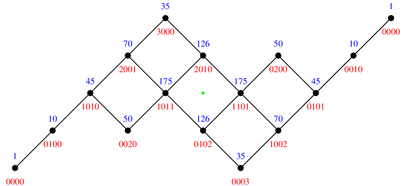
Figure 3. The ideal poset for $N_{5}^{+}=\operatorname{SO}(10)/\operatorname{U}(5)$. The upper label on each node is the dimension of the corresponding subrepresentation of $\Lambda^{*,0}\bigl{(}\operatorname{\mathfrak{so}}(10)/\operatorname{\mathfrak{u}}(5)\bigr{)}$ and the lower label is its highest weight as a representation of $\operatorname{SU}(5)$.

More detail about the topology and Schubert cell decomposition of $N^{+}_{m}$ can be found in [1]. Complete information about the irreducible constituents of the exterior powers of the cotangent bundle of $N^{+}_{m}$ and the consequent structure of its ideal poset is collected in a convenient form in [19]. The corresponding Hasse diagram for the case $m=5$ is drawn in Figure 3.

4.3.2. Ideals of degree $3$

I have not analyzed the minimal ideals in all dimensions for the isotropic Grassmannian, so I will confine myself to studying the cases in the first interesting degree, that of ideals of degree or codegree equal to $3$.

The first task is to describe the irreducible decomposition of $\Lambda^{3,0}(\operatorname{\mathfrak{m}})$ under the action of $K=\operatorname{U}(m)$. Fortunately, this is relatively easy. The above description of the tangent space to $N^{+}_{m}$ implies that, as a representation of $\operatorname{U}(m)$, the space $\operatorname{\mathfrak{m}}$ is isomorphic to the representation $\Lambda^{2}(\mathbb{C}^{\,m})={\mathbb{S}}_{(1,1)}(\mathbb{C}^{\,m})$ associated to the standard representation of $\operatorname{U}(m)$ on $\mathbb{C}^{\,m}$. Then a little work with multiplicity formulae from [9] shows that

(4.18) $$\Lambda^{3}\bigl{(}\Lambda^{2}(\mathbb{C}^{\,m})\bigr{)}\simeq\Lambda^{3}\bigl{(}{\mathbb{S}}_{(1,1)}(\mathbb{C}^{\,m})\bigr{)}\simeq{\mathbb{S}}_{(2,2,2)}(\mathbb{C}^{\,m})\oplus{\mathbb{S}}_{(3,1,1,1)}(\mathbb{C}^{\,m}).$$

These latter two representations are irreducible and their dimensions are given by [9, Theorem 6.3 or Exercise 6.4] as:

(4.19) $$\begin{split}\dim{\mathbb{S}}_{(2,2,2)}(\mathbb{C}^{\,m})&=\frac{m^{2}(m{-}1)^{2}(m{-}2)(m{+}1)}{144},\\ \dim{\mathbb{S}}_{(3,1,1,1)}(\mathbb{C}^{\,m})&=\frac{m(m^{2}{-}1)(m^{2}{-}4)(m{-}3)}{72}.\end{split}$$

Let ${\mathcal{I}}_{(2,2,2)}$ and ${\mathcal{I}}_{(3,1,1,1)}$, respectively, denote the exterior differential systems on $N^{+}_{m}$ generated in degree $3$ by the sections of ${\mathbb{S}}_{(2,2,2)}(S)\subset\Lambda^{3}(T^{*}N^{+}_{m})$ and ${\mathbb{S}}_{(3,1,1,1)}(S)\subset\Lambda^{3}(T^{*}N^{+}_{m})$.

4.3.3. Integral elements

The following linear algebra lemma identifies the integral elements of dimension three or more for each of the two $\operatorname{SL}(m,{\mathbb{C}})$-invariant subspaces of $\Lambda^{3}\bigl{(}\Lambda^{2}((\mathbb{C}^{\,m})^{*})\bigr{)}$.

Lemma 13.

Any subspace $E\subset\Lambda^{2}(\mathbb{C}^{\,m})$ of dimension $3$ or more on which all of the elements of ${\mathbb{S}}_{(2,2,2)}\bigl{(}(\mathbb{C}^{\,m})^{*}\bigr{)}$ vanish is of the form $E=L{\mathchoice{\,{\scriptstyle\wedge}\,}{{\scriptstyle\wedge}}{{\scriptscriptstyle\wedge}}{{\scriptscriptstyle\wedge}}}V$ where $L\subset\mathbb{C}^{\,m}$ is a line and $V\subset\mathbb{C}^{\,m}$ is a subspace containing $L$ whose dimension is one more than that of $E$.

Any subspace $E\subset\Lambda^{2}(\mathbb{C}^{\,m})$ of dimension $3$ or more on which all of the elements of ${\mathbb{S}}_{(3,1,1,1)}\bigl{(}(\mathbb{C}^{\,m})^{*}\bigr{)}$ vanish has dimension $3$ and is of the form $E=\Lambda^{2}(W)$ where $W\subset\mathbb{C}^{\,m}$ is a subspace of dimension $3$.

Proof.

Let $\eta:\Lambda^{2}(\mathbb{C}^{\,m})\to\Lambda^{2}(\mathbb{C}^{\,m})$ be the identity map. For any basis $\mathbf{v}_{1},\dots,\mathbf{v}_{m}$ of $\mathbb{C}^{\,m}$, write $\eta=\frac{1}{2}\eta^{ab}\mathbf{v}_{a}{\mathchoice{\,{\scriptstyle\wedge}\,}{{\scriptstyle\wedge}}{{\scriptscriptstyle\wedge}}{{\scriptscriptstyle\wedge}}}\mathbf{v}_{b}$, where $\eta^{ab}=-\eta^{ba}$ are 1-forms on $\Lambda^{2}(\mathbb{C}^{\,m})$. Note that $\{\eta^{ab}\mid a<b\}$ is a basis for the dual space.

Now, ${\mathbb{S}}_{(2,2,2)}(\mathbb{C}^{\,m})$ occurs as a constituent of $S^{2}(\mathbb{C}^{\,m})^{\otimes 3}$, but ${\mathbb{S}}_{(3,1,1,1)}(\mathbb{C}^{\,m})$ does not. Consequently, the $3$-forms of the form

(4.20) $$\psi(X,Y,Z)=X_{i_{1}i_{2}}Y_{i_{3}i_{4}}Z_{i_{5}i_{6}}\,\eta^{i_{1}i_{3}}{\mathchoice{\,{\scriptstyle\wedge}\,}{{\scriptstyle\wedge}}{{\scriptscriptstyle\wedge}}{{\scriptscriptstyle\wedge}}}\eta^{i_{2}i_{5}}{\mathchoice{\,{\scriptstyle\wedge}\,}{{\scriptstyle\wedge}}{{\scriptscriptstyle\wedge}}{{\scriptscriptstyle\wedge}}}\eta^{i_{4}i_{6}}\,,$$

when $X$, $Y$, and $Z$ are symmetric in their indices, must lie in ${\mathbb{S}}_{(2,2,2)}\bigl{(}(\mathbb{C}^{\,m})^{*}\bigr{)}\subset\Lambda^{3}\bigl{(}\Lambda^{2}((\mathbb{C}^{\,m})^{*})\bigr{)}$. Taking, as a particular example, $X_{11}=Y_{22}=Z_{33}=1$ and all other $X_{ij}$, $Y_{ij}$ and $Z_{ij}$ equal to zero yields $\psi(X,Y,Z)=\eta^{12}{\mathchoice{\,{\scriptstyle\wedge}\,}{{\scriptstyle\wedge}}{{\scriptscriptstyle\wedge}}{{\scriptscriptstyle\wedge}}}\eta^{13}{\mathchoice{\,{\scriptstyle\wedge}\,}{{\scriptstyle\wedge}}{{\scriptscriptstyle\wedge}}{{\scriptscriptstyle\wedge}}}\eta^{23}\not=0$, so the span of the $\psi(X,Y,Z)$ is nontrivial. Since this span is invariant under $\operatorname{GL}(m,{\mathbb{C}})$ and since ${\mathbb{S}}_{(2,2,2)}\bigl{(}(\mathbb{C}^{\,m})^{*}\bigr{)}$ is irreducible, this span must be all of this subspace. Thus, ${\mathbb{S}}_{(2,2,2)}\bigl{(}(\mathbb{C}^{\,m})^{*}\bigr{)}$ is the span of the $3$-forms of the form (4.20).

Now suppose that $E\subset\Lambda^{2}(\mathbb{C}^{\,m})$ is a subspace of dimension $d\geq 3$ on which all of the forms in ${\mathbb{S}}_{(2,2,2)}\bigl{(}(\mathbb{C}^{\,m})^{*}\bigr{)}$ vanish. My goal is to show that there is a unique line $L\subset\mathbb{C}^{\,m}$ so that $E\subset L{\mathchoice{\,{\scriptstyle\wedge}\,}{{\scriptstyle\wedge}}{{\scriptscriptstyle\wedge}}{{\scriptscriptstyle\wedge}}}\mathbb{C}^{\,m}$ and, conversely, that all of these $3$-forms vanish on $L{\mathchoice{\,{\scriptstyle\wedge}\,}{{\scriptstyle\wedge}}{{\scriptscriptstyle\wedge}}{{\scriptscriptstyle\wedge}}}\mathbb{C}^{\,m}$ for any line $L\subset\mathbb{C}^{\,m}$.

The converse assertion is easy, so let me do this first. Since all of the conditions are invariant under the action of $\operatorname{GL}(m,{\mathbb{C}})$, it suffices to prove this for the case that $L={\mathbb{C}}\,\mathbf{v}_{1}$. In this case, $E={\mathbb{C}}\,\mathbf{v}_{1}{\mathchoice{\,{\scriptstyle\wedge}\,}{{\scriptstyle\wedge}}{{\scriptscriptstyle\wedge}}{{\scriptscriptstyle\wedge}}}\mathbb{C}^{\,m}$ has dimension $m{-}1$ and is defined by the equations $\eta^{ab}=0$ when $1<a<b$, so suppose that all of these $1$-forms have been set to zero. Then for $\psi$ of the form (4.20), all of the terms vanish unless exactly one entry of each of the pairs $(i_{1},i_{3})$, $(i_{2},i_{5})$, and $(i_{4},i_{6})$ is equal to $1$. Moreover, the entries not equal to $1$ in these pairs must all be distinct.

Clearly, it suffices to treat the case where all of these entries are drawn from the set $\{1,2,3,4\}$. There are eight possible ways to assign the value of $1$ to one element of each of the pairs $(i_{1},i_{3})$, $(i_{2},i_{5})$, and $(i_{4},i_{6})$. In six of those ways, two of these indices will enter the same $X$, $Y$, or $Z$ coefficient and the corresponding sub-sum will vanish. For example, when $i_{1}=i_{2}=i_{4}=1$, the part of the sum in (4.20) corresponding to this choice is the sub-sum $X_{11}Y_{i_{3}1}Z_{i_{5}i_{6}}\,\eta^{1i_{3}}{\mathchoice{\,{\scriptstyle\wedge}\,}{{\scriptstyle\wedge}}{{\scriptscriptstyle\wedge}}{{\scriptscriptstyle\wedge}}}\eta^{1i_{5}}{\mathchoice{\,{\scriptstyle\wedge}\,}{{\scriptstyle\wedge}}{{\scriptscriptstyle\wedge}}{{\scriptscriptstyle\wedge}}}\eta^{1i_{6}}$, which vanishes, since $Z_{i_{5}i_{6}}$ is symmetric and $\eta^{1i_{5}}{\mathchoice{\,{\scriptstyle\wedge}\,}{{\scriptstyle\wedge}}{{\scriptscriptstyle\wedge}}{{\scriptscriptstyle\wedge}}}\eta^{1i_{6}}$ is skewsymmetric in the pair ${i_{5},i_{6}}$. The two exceptional configurations are $i_{1}=i_{4}=i_{5}=1$ and $i_{2}=i_{3}=i_{6}=1$, but these two sub-sums cancel:

$$X_{i_{1}1}Y_{1i_{4}}Z_{i_{5}1}\,\eta^{i_{1}1}{\mathchoice{\,{\scriptstyle\wedge}\,}{{\scriptstyle\wedge}}{{\scriptscriptstyle\wedge}}{{\scriptscriptstyle\wedge}}}\eta^{1i_{5}}{\mathchoice{\,{\scriptstyle\wedge}\,}{{\scriptstyle\wedge}}{{\scriptscriptstyle\wedge}}{{\scriptscriptstyle\wedge}}}\eta^{i_{4}1}+X_{1i_{2}}Y_{i_{3}1}Z_{1i_{6}}\,\eta^{1i_{3}}{\mathchoice{\,{\scriptstyle\wedge}\,}{{\scriptstyle\wedge}}{{\scriptscriptstyle\wedge}}{{\scriptscriptstyle\wedge}}}\eta^{i_{2}1}{\mathchoice{\,{\scriptstyle\wedge}\,}{{\scriptstyle\wedge}}{{\scriptscriptstyle\wedge}}{{\scriptscriptstyle\wedge}}}\eta^{1i_{6}}\\ =\quad X_{1i_{1}}Y_{1i_{4}}Z_{1i_{5}}\,\eta^{1i_{1}}{\mathchoice{\,{\scriptstyle\wedge}\,}{{\scriptstyle\wedge}}{{\scriptscriptstyle\wedge}}{{\scriptscriptstyle\wedge}}}\eta^{1i_{5}}{\mathchoice{\,{\scriptstyle\wedge}\,}{{\scriptstyle\wedge}}{{\scriptscriptstyle\wedge}}{{\scriptscriptstyle\wedge}}}\eta^{1i_{4}}-X_{1i_{2}}Y_{1i_{3}}Z_{1i_{6}}\,\eta^{1i_{3}}{\mathchoice{\,{\scriptstyle\wedge}\,}{{\scriptstyle\wedge}}{{\scriptscriptstyle\wedge}}{{\scriptscriptstyle\wedge}}}\eta^{1i_{2}}{\mathchoice{\,{\scriptstyle\wedge}\,}{{\scriptstyle\wedge}}{{\scriptscriptstyle\wedge}}{{\scriptscriptstyle\wedge}}}\eta^{1i_{6}}=0.$$

Thus, all the forms in ${\mathbb{S}}_{(2,2,2)}\bigl{(}(\mathbb{C}^{\,m})^{*}\bigr{)}$ vanish on $E=L{\mathchoice{\,{\scriptstyle\wedge}\,}{{\scriptstyle\wedge}}{{\scriptscriptstyle\wedge}}{{\scriptscriptstyle\wedge}}}\mathbb{C}^{\,m}$, as desired.

Now suppose that $E\subset\Lambda^{2}(\mathbb{C}^{\,m})$ is an integral element of ${\mathbb{S}}_{(2,2,2)}\bigl{(}(\mathbb{C}^{\,m})^{*}\bigr{)}$ and that $\dim E\geq 3$. Then $E$ will be defined by some set of linear relations among the 1-forms $\eta^{ab}$. (By hypothesis, however, at least three of the $\eta^{ab}$ are linearly independent on $E$.) My goal is to show that one can choose the basis $\mathbf{v}_{1},\dots,\mathbf{v}_{m}$ so that these relations include $\eta^{ab}=0$ for $a,b>1$.

Suppose that the basis $\mathbf{v}_{1},\dots,\mathbf{v}_{m}$ has been chosen so that the maximum number, say $p-1\geq 0$, of the forms $\eta^{12},\dots,\eta^{1m}$ are linearly independent on $E$. Clearly, $2\leq p\leq\dim E+1$. By making a change of basis in $\mathbf{v}_{2},\dots,\mathbf{v}_{m}$, I can assume that $\eta^{12}{\mathchoice{\,{\scriptstyle\wedge}\,}{{\scriptstyle\wedge}}{{\scriptscriptstyle\wedge}}{{\scriptscriptstyle\wedge}}}\dots\mathchoice{\,{\scriptstyle\wedge}\,}{{\scriptstyle\wedge}}{{\scriptscriptstyle\wedge}}{{\scriptscriptstyle\wedge}}\eta^{1p}\not=0$ on $E$ but that $\eta^{1a}=0$ on $E$ for $a>p$.

I claim that the maximality property implies that $\eta^{ab}\equiv 0\mod\eta^{12},\dots,\eta^{1p}$ whenever $a>p$. To see this, let $\lambda_{2},\dots,\lambda_{m}$ be parameters and consider the basis $\mathbf{v}_{1},\mathbf{v}^{*}_{2},\dots,\mathbf{v}^{*}_{m}$ defined by $\mathbf{v}^{*}_{a}=\mathbf{v}_{a}-\lambda_{a}\,\mathbf{v}_{1}$ for $a>1$. Then

$$\eta=\frac{1}{2}\,\eta^{ab}\,\mathbf{v}_{a}{\mathchoice{\,{\scriptstyle\wedge}\,}{{\scriptstyle\wedge}}{{\scriptscriptstyle\wedge}}{{\scriptscriptstyle\wedge}}}\mathbf{v}_{b}=\sum_{1<a}(\eta^{1a}+\lambda_{b}\eta^{ba})\,\mathbf{v}_{1}{\mathchoice{\,{\scriptstyle\wedge}\,}{{\scriptstyle\wedge}}{{\scriptscriptstyle\wedge}}{{\scriptscriptstyle\wedge}}}\mathbf{v}^{*}_{a}+\frac{1}{2}\sum_{1<a,b}\eta^{ab}\,\mathbf{v}^{*}_{a}{\mathchoice{\,{\scriptstyle\wedge}\,}{{\scriptstyle\wedge}}{{\scriptscriptstyle\wedge}}{{\scriptscriptstyle\wedge}}}\mathbf{v}^{*}_{b}\,.$$

Suppose that there exist $q>p$ and $r>1$ so that  $\eta^{12}{\mathchoice{\,{\scriptstyle\wedge}\,}{{\scriptstyle\wedge}}{{\scriptscriptstyle\wedge}}{{\scriptscriptstyle\wedge}}}\dots\mathchoice{\,{\scriptstyle\wedge}\,}{{\scriptstyle\wedge}}{{\scriptscriptstyle\wedge}}{{\scriptscriptstyle\wedge}}\eta^{1p}{\mathchoice{\,{\scriptstyle\wedge}\,}{{\scriptstyle\wedge}}{{\scriptscriptstyle\wedge}}{{\scriptscriptstyle\wedge}}}\eta^{qr}\not=0$. Then set $\lambda_{a}=0$ for $a\not=r$ and $\lambda_{r}=t$ and consider the expansion

$$(\eta^{12}{+}t\eta^{r2}){\mathchoice{\,{\scriptstyle\wedge}\,}{{\scriptstyle\wedge}}{{\scriptscriptstyle\wedge}}{{\scriptscriptstyle\wedge}}}\dots\mathchoice{\,{\scriptstyle\wedge}\,}{{\scriptstyle\wedge}}{{\scriptscriptstyle\wedge}}{{\scriptscriptstyle\wedge}}(\eta^{1p}{+}t\eta^{rp}){\mathchoice{\,{\scriptstyle\wedge}\,}{{\scriptstyle\wedge}}{{\scriptscriptstyle\wedge}}{{\scriptscriptstyle\wedge}}}(\eta^{1q}{+}t\eta^{rq})=t\,\eta^{12}{{\mathchoice{\,{\scriptstyle\wedge}\,}{{\scriptstyle\wedge}}{{\scriptscriptstyle\wedge}}{{\scriptscriptstyle\wedge}}}}\dots{\mathchoice{\,{\scriptstyle\wedge}\,}{{\scriptstyle\wedge}}{{\scriptscriptstyle\wedge}}{{\scriptscriptstyle\wedge}}}\eta^{1p}{{\mathchoice{\,{\scriptstyle\wedge}\,}{{\scriptstyle\wedge}}{{\scriptscriptstyle\wedge}}{{\scriptscriptstyle\wedge}}}}\eta^{rq}+O({t}^{2})$$

Clearly, there will be a nonempty open set of values for $t$ for which the left hand side of this equation will be nonzero, thus contradicting the maximality of $p$.

It follows immediately that $p\geq 3$. Now, so far, no use has been made of the hypothesis that $E$ be an integral element of ${\mathbb{S}}_{(2,2,2)}\bigl{(}(\mathbb{C}^{\,m})^{*}\bigr{)}$. Its first use is to show that $p\geq 4$. This follows because, as has already been noted, one of the elements of ${\mathbb{S}}_{(2,2,2)}\bigl{(}(\mathbb{C}^{\,m})^{*}\bigr{)}$ is $\eta^{12}{\mathchoice{\,{\scriptstyle\wedge}\,}{{\scriptstyle\wedge}}{{\scriptscriptstyle\wedge}}{{\scriptscriptstyle\wedge}}}\eta^{13}{\mathchoice{\,{\scriptstyle\wedge}\,}{{\scriptstyle\wedge}}{{\scriptscriptstyle\wedge}}{{\scriptscriptstyle\wedge}}}\eta^{23}$. Since $\eta^{12}{\mathchoice{\,{\scriptstyle\wedge}\,}{{\scriptstyle\wedge}}{{\scriptscriptstyle\wedge}}{{\scriptscriptstyle\wedge}}}\eta^{13}\not=0$, it follows that $\eta^{23}$ is a linear combination of $\eta^{12}$ and $\eta^{13}$. If it were true that $p=3$, then all of the forms $\eta^{ab}$ with $a>3$ would also be linear combinations of $\eta^{12}$ and $\eta^{13}$, so there could not be three linearly independent $1$-forms among the $\eta^{ab}$. Thus, $p\geq 4$, as claimed.

Now, the same argument that showed that $\eta^{12}{\mathchoice{\,{\scriptstyle\wedge}\,}{{\scriptstyle\wedge}}{{\scriptscriptstyle\wedge}}{{\scriptscriptstyle\wedge}}}\eta^{13}{\mathchoice{\,{\scriptstyle\wedge}\,}{{\scriptstyle\wedge}}{{\scriptscriptstyle\wedge}}{{\scriptscriptstyle\wedge}}}\eta^{23}$ is in ${\mathbb{S}}_{(2,2,2)}\bigl{(}(\mathbb{C}^{\,m})^{*}\bigr{)}$ shows that $\eta^{1a}{\mathchoice{\,{\scriptstyle\wedge}\,}{{\scriptstyle\wedge}}{{\scriptscriptstyle\wedge}}{{\scriptscriptstyle\wedge}}}\eta^{1b}{\mathchoice{\,{\scriptstyle\wedge}\,}{{\scriptstyle\wedge}}{{\scriptscriptstyle\wedge}}{{\scriptscriptstyle\wedge}}}\eta^{ab}$ is in ${\mathbb{S}}_{(2,2,2)}\bigl{(}(\mathbb{C}^{\,m})^{*}\bigr{)}$ for all $1<a<b$. In particular, it follows that $\eta^{ab}\equiv 0\mod~{}\eta^{12},\dots,\eta^{1p}$ for all $a,b\leq p$. Combined with the previous argument, showing that $\eta^{ab}\equiv 0\mod~{}\eta^{12},\dots,\eta^{1p}$ when either $a$ or $b$ is greater than $p$, this shows that $\eta^{12},\dots,\eta^{1p}$ must actually be a basis for the 1-forms on $E$, i.e., $p=\dim E+1$.

Now, the fact that $\eta^{1a}{\mathchoice{\,{\scriptstyle\wedge}\,}{{\scriptstyle\wedge}}{{\scriptscriptstyle\wedge}}{{\scriptscriptstyle\wedge}}}\eta^{1b}{\mathchoice{\,{\scriptstyle\wedge}\,}{{\scriptstyle\wedge}}{{\scriptscriptstyle\wedge}}{{\scriptscriptstyle\wedge}}}\eta^{ab}=0$ on $E$ for $a,b\leq p$ combined with the skew-symmetry $\eta^{ab}=-\eta^{ba}$ implies that there exist unique numbers $A_{ab}$ for $1<a\not=b\leq p$ so that

$$\eta^{ab}=A^{ab}\eta^{1a}-A^{ba}\eta^{1b}.$$

Moreover, for any distinct $a,b,c$ satisfying $1<a,b,c\leq p$, the formula (4.20) shows that the form

$$\eta^{1a}{\mathchoice{\,{\scriptstyle\wedge}\,}{{\scriptstyle\wedge}}{{\scriptscriptstyle\wedge}}{{\scriptscriptstyle\wedge}}}\eta^{1b}{\mathchoice{\,{\scriptstyle\wedge}\,}{{\scriptstyle\wedge}}{{\scriptscriptstyle\wedge}}{{\scriptscriptstyle\wedge}}}\eta^{ac}+\eta^{1a}{\mathchoice{\,{\scriptstyle\wedge}\,}{{\scriptstyle\wedge}}{{\scriptscriptstyle\wedge}}{{\scriptscriptstyle\wedge}}}\eta^{1c}{\mathchoice{\,{\scriptstyle\wedge}\,}{{\scriptstyle\wedge}}{{\scriptscriptstyle\wedge}}{{\scriptscriptstyle\wedge}}}\eta^{ab}$$

lies in ${\mathbb{S}}_{(2,2,2)}\bigl{(}(\mathbb{C}^{\,m})^{*}\bigr{)}$, so the fact that this vanishes on $E$ implies that $A^{ca}=A^{ba}$. It follows that there are constants $A^{a}$ so that $A^{ba}=A^{a}$ for all $b\not=a$. Consequently, $\eta^{ab}=A^{b}\eta^{1a}-A^{a}\eta^{1b}$ for  $1<a,b\leq p$. Thus, by replacing $\mathbf{v}_{1}$ by $\mathbf{v}_{1}+A^{b}\,\mathbf{v}_{b}$, I get a new basis in which $\eta^{ab}=0$ holds on $E$ for $1<a,b\leq p$, so I assume this from now on.

Next, taking $a,b,c$ satisfying $1<a<b\leq p<c$, the above form simplifies on $E$ to $\eta^{1a}{\mathchoice{\,{\scriptstyle\wedge}\,}{{\scriptstyle\wedge}}{{\scriptscriptstyle\wedge}}{{\scriptscriptstyle\wedge}}}\eta^{1b}{\mathchoice{\,{\scriptstyle\wedge}\,}{{\scriptstyle\wedge}}{{\scriptscriptstyle\wedge}}{{\scriptscriptstyle\wedge}}}\eta^{ac}$. Since this must vanish, it follows that $\eta^{ac}\equiv 0\mod\eta^{1a},\eta^{1b}$ for all such triples. Since $p\geq 4$, this implies $\eta^{ac}\equiv 0\mod\eta^{1a}$ whenever $1<a\leq p<c$. Thus, set $\eta^{ac}=B^{ac}\eta^{1a}$ for some quantities $B^{ac}$.

Now, observe that the sum

$$\eta^{1a}{\mathchoice{\,{\scriptstyle\wedge}\,}{{\scriptstyle\wedge}}{{\scriptscriptstyle\wedge}}{{\scriptscriptstyle\wedge}}}\eta^{1b}{\mathchoice{\,{\scriptstyle\wedge}\,}{{\scriptstyle\wedge}}{{\scriptscriptstyle\wedge}}{{\scriptscriptstyle\wedge}}}\eta^{dc}+\eta^{1d}{\mathchoice{\,{\scriptstyle\wedge}\,}{{\scriptstyle\wedge}}{{\scriptscriptstyle\wedge}}{{\scriptscriptstyle\wedge}}}\eta^{1b}{\mathchoice{\,{\scriptstyle\wedge}\,}{{\scriptstyle\wedge}}{{\scriptscriptstyle\wedge}}{{\scriptscriptstyle\wedge}}}\eta^{ac}+\eta^{1a}{\mathchoice{\,{\scriptstyle\wedge}\,}{{\scriptstyle\wedge}}{{\scriptscriptstyle\wedge}}{{\scriptscriptstyle\wedge}}}\eta^{1c}{\mathchoice{\,{\scriptstyle\wedge}\,}{{\scriptstyle\wedge}}{{\scriptscriptstyle\wedge}}{{\scriptscriptstyle\wedge}}}\eta^{db}+\eta^{1d}{\mathchoice{\,{\scriptstyle\wedge}\,}{{\scriptstyle\wedge}}{{\scriptscriptstyle\wedge}}{{\scriptscriptstyle\wedge}}}\eta^{1c}{\mathchoice{\,{\scriptstyle\wedge}\,}{{\scriptstyle\wedge}}{{\scriptscriptstyle\wedge}}{{\scriptscriptstyle\wedge}}}\eta^{ab}$$

is in ${\mathbb{S}}_{(2,2,2)}\bigl{(}(\mathbb{C}^{\,m})^{*}\bigr{)}$, and take $1<a<d\leq p$ and $1<b\leq p<c$ with $b$ not equal to either $a$ or $d$. (This last is possible since $p\geq 4$.) The last two terms in the sum vanish since $\eta^{1c}=0$ and the first two terms simplify to $(B^{dc}-B^{ac})\,\eta^{1a}{\mathchoice{\,{\scriptstyle\wedge}\,}{{\scriptstyle\wedge}}{{\scriptscriptstyle\wedge}}{{\scriptscriptstyle\wedge}}}\eta^{1b}{\mathchoice{\,{\scriptstyle\wedge}\,}{{\scriptstyle\wedge}}{{\scriptscriptstyle\wedge}}{{\scriptscriptstyle\wedge}}}\eta^{1d}$. Since this must vanish, it follows that $B^{ac}=B^{c}$ for some constants $B^{c}$ when $c>p$. Thus, $\eta^{ac}=B^{c}\eta^{1a}$. It follows that, by replacing $\mathbf{v}_{1}$ by $\mathbf{v}_{1}+B^{c}\mathbf{v}_{c}$, I can arrange that $\eta^{ac}=0$ whenever $1<a\leq p<c$, so assume this from now on.

Finally, go back to the above sum and assume $1<a<b\leq p<d<c$. Then all of the terms except the first are zero. The vanishing of the first term $\eta^{1a}{\mathchoice{\,{\scriptstyle\wedge}\,}{{\scriptstyle\wedge}}{{\scriptscriptstyle\wedge}}{{\scriptscriptstyle\wedge}}}\eta^{1b}{\mathchoice{\,{\scriptstyle\wedge}\,}{{\scriptstyle\wedge}}{{\scriptscriptstyle\wedge}}{{\scriptscriptstyle\wedge}}}\eta^{dc}$ implies that $\eta^{dc}$ is a linear combination of $\eta^{1a}$ and $\eta^{1b}$ for any distinct pair of indices $a$ and $b$ satisfying $1<a<b\leq p$. Since $p\geq 4$, this forces $\eta^{dc}=0$.

Thus $E$ satisfies the relations $\eta^{ab}=0$ for $1<a,b\leq m$ and for $a=1$ and $b>p=\dim E+1$. It follows that $\mathbf{v}_{1}{\mathchoice{\,{\scriptstyle\wedge}\,}{{\scriptstyle\wedge}}{{\scriptscriptstyle\wedge}}{{\scriptscriptstyle\wedge}}}\mathbf{v}_{2},\dots,\mathbf{v}_{1}{\mathchoice{\,{\scriptstyle\wedge}\,}{{\scriptstyle\wedge}}{{\scriptscriptstyle\wedge}}{{\scriptscriptstyle\wedge}}}\mathbf{v}_{p}$ is a basis for $E$, as desired.

Now, I will compute the integral elements of ${\mathbb{S}}_{(3,1,1,1)}\bigl{(}(\mathbb{C}^{\,m})^{*}\bigr{)}$. My goal is to show that any integral element $E$ of dimension $3$ or more is actually of the form $E=\Lambda^{2}(W)$ for some (unique) $3$-dimensional subspace $W\subset\mathbb{C}^{\,m}$.

First, I must describe a set of generators of ${\mathbb{S}}_{(3,1,1,1)}\bigl{(}(\mathbb{C}^{\,m})^{*}\bigr{)}$. Now, it is easy to calculate that ${\mathbb{S}}_{(3,1,1,1)}\bigl{(}(\mathbb{C}^{\,m})^{*}\bigr{)}$ occurs as a constituent of $\Lambda^{4}\bigl{(}(\mathbb{C}^{\,m})^{*}\bigr{)}\otimes S^{2}\bigl{(}(\mathbb{C}^{\,m})^{*}\bigr{)}$, but that ${\mathbb{S}}_{(2,2,2)}\bigl{(}(\mathbb{C}^{\,m})^{*}\bigr{)}$ does not. Consequently, every $3$-form of the form

(4.21) $$\psi(X,Y)=X_{i_{1}i_{2}i_{3}i_{4}}Y_{j_{1}j_{2}}\,\eta^{i_{1}i_{2}}{\mathchoice{\,{\scriptstyle\wedge}\,}{{\scriptstyle\wedge}}{{\scriptscriptstyle\wedge}}{{\scriptscriptstyle\wedge}}}\eta^{i_{3}j_{1}}{\mathchoice{\,{\scriptstyle\wedge}\,}{{\scriptstyle\wedge}}{{\scriptscriptstyle\wedge}}{{\scriptscriptstyle\wedge}}}\eta^{i_{4}j_{2}}$$

when $X$ is skewsymmetric in its indices and  $Y$ is symmetric in its indices, must actually lie in ${\mathbb{S}}_{(3,1,1,1)}\bigl{(}(\mathbb{C}^{\,m})^{*}\bigr{)}$. Taking, as particular examples, $Y_{ij}=\delta^{1}_{i}\delta^{1}_{j}$ and letting $X_{ijkl}$ be zero unless $\{i,j,k,l\}=\{1,2,3,4\}$ while $X_{1234}=1$, gives $\psi(X,Y)=24\,\eta^{12}{\mathchoice{\,{\scriptstyle\wedge}\,}{{\scriptstyle\wedge}}{{\scriptscriptstyle\wedge}}{{\scriptscriptstyle\wedge}}}\eta^{13}{\mathchoice{\,{\scriptstyle\wedge}\,}{{\scriptstyle\wedge}}{{\scriptscriptstyle\wedge}}{{\scriptscriptstyle\wedge}}}\eta^{14}\not=0$, so it follows that the $\psi(X,Y)$ span a nontrivial subspace of ${\mathbb{S}}_{(3,1,1,1)}\bigl{(}(\mathbb{C}^{\,m})^{*}\bigr{)}$. Since this subspace is evidently invariant under $\operatorname{GL}(m,{\mathbb{C}})$ and since ${\mathbb{S}}_{(3,1,1,1)}\bigl{(}(\mathbb{C}^{\,m})^{*}\bigr{)}$ is irreducible, it follows that the forms $\psi(X,Y)$ of the form (4.21) must span ${\mathbb{S}}_{(3,1,1,1)}\bigl{(}(\mathbb{C}^{\,m})^{*}\bigr{)}$.

Now suppose that $E\subset\Lambda^{2}(\mathbb{C}^{\,m})$ is an integral element of ${\mathbb{S}}_{(3,1,1,1)}\bigl{(}(\mathbb{C}^{\,m})^{*}\bigr{)}$ whose dimension is at least $3$. Just as in the first part of the argument, choose a basis $\mathbf{v}_{1},\dots,\mathbf{v}_{m}$ of $\mathbb{C}^{\,m}$ so that the maximum number, say, $p{-}1$, of $\{\eta^{12},\dots,\eta^{1m}\}$ are linearly independent on $E$ and so that $\eta^{1a}=0$ for $a>p$. The argument given in the first half of the proof shows that $p\geq 3$, but the fact that $\eta^{12}{\mathchoice{\,{\scriptstyle\wedge}\,}{{\scriptstyle\wedge}}{{\scriptscriptstyle\wedge}}{{\scriptscriptstyle\wedge}}}\eta^{13}{\mathchoice{\,{\scriptstyle\wedge}\,}{{\scriptstyle\wedge}}{{\scriptscriptstyle\wedge}}{{\scriptscriptstyle\wedge}}}\eta^{14}$ lies in ${\mathbb{S}}_{(3,1,1,1)}\bigl{(}(\mathbb{C}^{\,m})^{*}\bigr{)}$ implies that $p<4$. Thus, $p=3$. As before, the fact that $p=3$ is maximal implies that $\eta^{ab}\equiv 0\mod\eta^{12},\eta^{13}$ whenever $a>3$. In particular, all the 1-forms on $E$ must be linear combinations of $\eta^{12}$, $\eta^{13}$, and $\eta^{23}$. Consequently, $\dim E\leq 3$, but since $\dim E\geq 3$ by hypothesis, $\dim E=3$. Moreover, since there must be at least three linearly independent forms on $E$, it follows that $\eta^{12}{\mathchoice{\,{\scriptstyle\wedge}\,}{{\scriptstyle\wedge}}{{\scriptscriptstyle\wedge}}{{\scriptscriptstyle\wedge}}}\eta^{13}{\mathchoice{\,{\scriptstyle\wedge}\,}{{\scriptstyle\wedge}}{{\scriptscriptstyle\wedge}}{{\scriptscriptstyle\wedge}}}\eta^{23}\not=0$.

Now, the same argument as showed that there cannot be more than two independent forms among the $\eta^{1a}$ shows that there cannot be more than two independent forms among the $\eta^{2a}$ or the $\eta^{3a}$. In particular, for $a>3$, the $1$-form $\eta^{2a}$ must be a linear combination of $\eta^{21}$ and $\eta^{23}$. However, I have already shown that it must also be a linear combination of $\eta^{12}$ and $\eta^{13}$. Consequently $\eta^{2a}$ must simply be a multiple of $\eta^{21}$, say $\eta^{2a}=A^{2a}\,\eta^{21}$ for $a>3$. Similarly, $\eta^{3a}$ must simply be a multiple of $\eta^{31}$, say $\eta^{3a}=A^{3a}\,\eta^{31}$ for $a>3$.

Now, replacing $\mathbf{v}_{1}$ by $\mathbf{v}_{1}+\sum_{a>3}A^{2a}\mathbf{v}_{a}$ produces a new basis for which $\eta^{2a}=0$ for $a>3$, so assume that this has been done. Now, for each $a>3$, consider $\psi(X,Y)$ as in (4.21) where $X_{123a}=1$ while $X_{ijkl}=0$ unless $\{i,j,k,l\}=\{1,2,3,a\}$ and $Y_{23}=Y_{32}=1$ while $Y_{ij}=0$ unless $\{i,j\}=\{2,3\}$. The result is

$$\psi(X,Y)=4\,\eta^{12}{\mathchoice{\,{\scriptstyle\wedge}\,}{{\scriptstyle\wedge}}{{\scriptscriptstyle\wedge}}{{\scriptscriptstyle\wedge}}}\eta^{23}{\mathchoice{\,{\scriptstyle\wedge}\,}{{\scriptstyle\wedge}}{{\scriptscriptstyle\wedge}}{{\scriptscriptstyle\wedge}}}\eta^{3a}-4\,\eta^{13}{\mathchoice{\,{\scriptstyle\wedge}\,}{{\scriptstyle\wedge}}{{\scriptscriptstyle\wedge}}{{\scriptscriptstyle\wedge}}}\eta^{23}{\mathchoice{\,{\scriptstyle\wedge}\,}{{\scriptstyle\wedge}}{{\scriptscriptstyle\wedge}}{{\scriptscriptstyle\wedge}}}\eta^{2a}.$$

Since $\eta^{2a}=0$ on $E$, the vanishing of $\psi(X,Y)$ on $E$ forces $\eta^{3a}$ to be a linear combination of $\eta^{12}$ and $\eta^{23}$. Since $\eta^{3a}=A^{3a}\,\eta^{31}$, this forces $A^{3a}=0$, i.e., $\eta^{3a}$ vanishes on $E$.

If $m=4$, it has now been demonstrated that, for any integral $3$-dimensional integral element of ${\mathbb{S}}_{(3,1,1,1)}\bigl{(}(\mathbb{C}^{\,m})^{*}\bigr{)}$, there is a basis $\mathbf{v}_{1},\dots,\mathbf{v}_{m}$ so that $E$ is defined by the equations $\eta^{ab}=0$ when $a>3$.

If $m>4$ assume $a>b>3$ and consider $\psi(X,Y)$ where $X_{12ab}=1$ while $X_{ijkl}=0$ unless $\{i,j,k,l\}=\{1,2,a,b\}$ and $Y_{33}=1$ while $Y_{ij}=0$ unless $i=j=3$. Then, on $E$, $\psi(X,Y)=4\,\eta^{13}{\mathchoice{\,{\scriptstyle\wedge}\,}{{\scriptstyle\wedge}}{{\scriptscriptstyle\wedge}}{{\scriptscriptstyle\wedge}}}\eta^{23}{\mathchoice{\,{\scriptstyle\wedge}\,}{{\scriptstyle\wedge}}{{\scriptscriptstyle\wedge}}{{\scriptscriptstyle\wedge}}}\eta^{ab}=0$. Now, permuting $(1,2,3)$ in this construction shows that

$$\eta^{13}{\mathchoice{\,{\scriptstyle\wedge}\,}{{\scriptstyle\wedge}}{{\scriptscriptstyle\wedge}}{{\scriptscriptstyle\wedge}}}\eta^{23}{\mathchoice{\,{\scriptstyle\wedge}\,}{{\scriptstyle\wedge}}{{\scriptscriptstyle\wedge}}{{\scriptscriptstyle\wedge}}}\eta^{ab}=\eta^{23}{\mathchoice{\,{\scriptstyle\wedge}\,}{{\scriptstyle\wedge}}{{\scriptscriptstyle\wedge}}{{\scriptscriptstyle\wedge}}}\eta^{12}{\mathchoice{\,{\scriptstyle\wedge}\,}{{\scriptstyle\wedge}}{{\scriptscriptstyle\wedge}}{{\scriptscriptstyle\wedge}}}\eta^{ab}=\eta^{12}{\mathchoice{\,{\scriptstyle\wedge}\,}{{\scriptstyle\wedge}}{{\scriptscriptstyle\wedge}}{{\scriptscriptstyle\wedge}}}\eta^{13}{\mathchoice{\,{\scriptstyle\wedge}\,}{{\scriptstyle\wedge}}{{\scriptscriptstyle\wedge}}{{\scriptscriptstyle\wedge}}}\eta^{ab}=0.$$

This implies that $\eta^{ab}=0$, on $E$, as desired.

Finally, if there is a basis $\mathbf{v}_{1},\dots,\mathbf{v}_{m}$ so that $E$ is defined by $\eta^{ab}=0$ when $a>3$, then it is clear that $\psi(X,Y)$ vanishes on $E$ for all $X$ and $Y$, so that $E$ is, indeed, an integral element of ${\mathbb{S}}_{(3,1,1,1)}\bigl{(}(\mathbb{C}^{\,m})^{*}\bigr{)}$. ∎

4.3.4. Integral varieties

The next two propositions describe the integral manifolds of the exterior differential systems ${\mathcal{I}}_{(2,2,2)}$ and ${\mathcal{I}}_{(3,1,1,1)}$.

Before stating the first of these two propositions, I need to describe a family of projective spaces ${\mathbb{P}}^{m-1}$ that are embedded in $N^{+}_{m}$.

Example 21 (The chiral double fibration).

If $H\subset\mathbb{C}^{\,2m}$ is any isotropic $(m{-}1)$-plane, it lies in two distinct isotropic $m$-planes: $H^{+}$, of positive chirality, and $H^{-}$, of negative chirality. Thus, if $N_{m-1}(\mathbb{C}^{\,2m})\subset\operatorname{Gr}(m{-}1,2m)$ denotes the space of isotropic $(m{-}1)$-planes in $\mathbb{C}^{\,2m}$, this space is the apex of a double fibration

$$\begin{array}[]{ccccc}&&N_{m-1}(\mathbb{C}^{\,2m})\\ &\swarrow&&\searrow\\ N^{+}_{m}&&&&N^{-}_{m}\end{array}.$$

Let $S\subset\mathbb{C}^{\,2m}$ be any isotropic $m$-plane of negative chirality. Then there is a canonical embedding $\iota_{S}$ of ${\mathbb{P}}(S^{*})\simeq{\mathbb{P}}^{m-1}$ into $N^{+}_{m}$ defined by sending each hyperplane $H\in{\mathbb{P}}(S^{*})=\operatorname{Gr}(m{-}1,S)$ to its positive chirality extension $H^{+}=\iota_{S}(H)$.

Proposition 9.

For any $S\in N^{-}_{m}$, the projective space $\iota_{S}\bigl{(}{\mathbb{P}}(S^{*})\bigr{)}$ is a (maximal) integral manifold of ${\mathcal{I}}_{(2,2,2)}$.

Conversely, if $X\subset N^{+}_{m}$ is an irreducible variety of dimension at least $3$ that is an integral variety of ${\mathcal{I}}_{(2,2,2)}$, then there exists a unique $S\in N^{-}_{m}$ so that $X$ is contained in $\iota_{S}\bigl{(}{\mathbb{P}}(S^{*})\bigr{)}$.

Proof.

The first task (which will be needed in the next proposition as well), is to establish the equations of the moving frame for submanifolds of $N^{+}_{m}$.

Define $\operatorname{SO}(2m,{\mathbb{C}})$ be the subgroup of $\operatorname{SL}(2m,{\mathbb{C}})$ consisting of the matrices $\mathsf{u}$ that satisfy

(4.22) $${}^{t}\mathsf{u}\begin{pmatrix}0_{m}&\operatorname{I}_{m}\\ \operatorname{I}_{m}&0_{m}\end{pmatrix}\mathsf{u}=\begin{pmatrix}0_{m}&\operatorname{I}_{m}\\ \operatorname{I}_{m}&0_{m}\end{pmatrix}.$$

Also, let $F\subset\operatorname{GL}(2m,{\mathbb{C}})$ denote the set of matrices $\mathsf{v}$ that satisfy

(4.23) $${}^{t}\mathsf{v}\,\mathsf{v}=\begin{pmatrix}0_{m}&\operatorname{I}_{m}\\ \operatorname{I}_{m}&0_{m}\end{pmatrix}$$

and $\det(\mathsf{v})=\mathrm{i}^{m}$. Evidently, $F$ is an orbit of $\operatorname{SO}(2m,{\mathbb{C}})$ acting on $\operatorname{GL}(2m,{\mathbb{C}})$ on the right. I will regard $\mathsf{v}:F\to\operatorname{GL}(2m,{\mathbb{C}})$ as a matrix-valued function and denote its columns as

$$\mathsf{v}=(\mathsf{v}_{1}\quad\dots\quad\mathsf{v}_{m}\quad\mathsf{v}^{1}\quad\dots\quad\mathsf{v}^{m})$$

where $\mathsf{v}_{i},\mathsf{v}^{i}:F\to\mathbb{C}^{\,2m}$ are regarded as (holomorphic) mappings.

Define

$$\pi(\mathsf{v})=[\mathsf{v}_{1}{\mathchoice{\,{\scriptstyle\wedge}\,}{{\scriptstyle\wedge}}{{\scriptscriptstyle\wedge}}{{\scriptscriptstyle\wedge}}}\dots\mathchoice{\,{\scriptstyle\wedge}\,}{{\scriptstyle\wedge}}{{\scriptscriptstyle\wedge}}{{\scriptscriptstyle\wedge}}\mathsf{v}_{m}]\,,$$

so that $\pi$ is a surjective submersion $\pi:F\to N^{+}_{m}$. The fibers of $\pi$ are the orbits of the parabolic subgroup $P\subset\operatorname{SO}(2m,{\mathbb{C}})$ consisting of elements of the form

(4.24) $$\mathsf{u}=\begin{pmatrix}A&AB\\ 0_{m}&{}^{t}\!A^{-1}\end{pmatrix}\qquad\text{for~{}$A\in\operatorname{GL}(m,{\mathbb{C}})$ and~{}$B=-{}^{t}\!B\in\mathbb{C}^{\,m,m}$.}$$

Thus, $\pi:F\to N^{+}_{m}$ is a principal right $P$-bundle over $N^{+}_{m}$.

In accordance with the usual moving frame conventions, write the structure equations as

(4.25) $$\mathrm{d}\mathsf{v}=\mathrm{d}(\mathsf{v}_{i}\ \mathsf{v}^{i})=(\mathsf{v}_{j}\ \mathsf{v}^{j})\begin{pmatrix}\alpha^{j}_{i}&\gamma^{ji}\\ \beta_{ji}&-\alpha^{i}_{j}\end{pmatrix}=\mathsf{v}\,\theta$$

where

(4.26) $$\beta_{ji}=-\beta_{ij}\quad\text{and}\quad\gamma^{ji}=-\gamma^{ij}\,,$$

but the components of $\alpha$, $\beta$, and $\gamma$ are otherwise linearly independent. The relations (4.26) follow in the usual way from the exterior derivative of (4.23). The structure equation $\mathrm{d}\theta=-\theta{\mathchoice{\,{\scriptstyle\wedge}\,}{{\scriptstyle\wedge}}{{\scriptscriptstyle\wedge}}{{\scriptscriptstyle\wedge}}}\theta$ holds since $\theta=\mathsf{v}^{-1}\,\mathrm{d}\mathsf{v}$. These expand to

(4.27) $$\begin{split}\mathrm{d}\alpha^{i}_{j}&=-\alpha^{i}_{k}{\mathchoice{\,{\scriptstyle\wedge}\,}{{\scriptstyle\wedge}}{{\scriptscriptstyle\wedge}}{{\scriptscriptstyle\wedge}}}\alpha^{k}_{j}-\gamma^{ik}{\mathchoice{\,{\scriptstyle\wedge}\,}{{\scriptstyle\wedge}}{{\scriptscriptstyle\wedge}}{{\scriptscriptstyle\wedge}}}\beta_{kj}\,,\\ \mathrm{d}\beta_{ij}&=-\beta_{ik}{\mathchoice{\,{\scriptstyle\wedge}\,}{{\scriptstyle\wedge}}{{\scriptscriptstyle\wedge}}{{\scriptscriptstyle\wedge}}}\alpha^{k}_{j}+\alpha^{k}_{i}{\mathchoice{\,{\scriptstyle\wedge}\,}{{\scriptstyle\wedge}}{{\scriptscriptstyle\wedge}}{{\scriptscriptstyle\wedge}}}\beta_{kj}\,,\\ \mathrm{d}\gamma^{ij}&=-\alpha^{i}_{k}{\mathchoice{\,{\scriptstyle\wedge}\,}{{\scriptstyle\wedge}}{{\scriptscriptstyle\wedge}}{{\scriptscriptstyle\wedge}}}\gamma^{kj}+\gamma^{ik}{\mathchoice{\,{\scriptstyle\wedge}\,}{{\scriptstyle\wedge}}{{\scriptscriptstyle\wedge}}{{\scriptscriptstyle\wedge}}}\alpha^{j}_{k}\,.\end{split}$$

Now suppose that $X\subset N^{+}_{m}$ is an irreducible integral variety of ${\mathcal{I}}_{(2,2,2)}$ of dimension $d\geq 3$, and let $X^{\circ}\subset X$ denote its smooth locus, which is an embedded submanifold of $N^{+}_{m}$. For every $V\in X^{\circ}$, the tangent space $T_{V}X$ is an integral element of ${\mathcal{I}}_{(2,2,2)}$ of dimension $d\geq 3$. By Lemma 13, it follows that, for every $V\in X^{\circ}$, there exists a $\mathsf{v}\in F$ so that

1. $V$ is spanned by $\mathsf{v}_{1},\dots,\mathsf{v}_{m}$, and

2. $T_{V}X$ is spanned by $[\![\mathsf{v}^{1}]\!]{\mathchoice{\,{\scriptstyle\wedge}\,}{{\scriptstyle\wedge}}{{\scriptscriptstyle\wedge}}{{\scriptscriptstyle\wedge}}}[\![\mathsf{v}^{2}]\!],[\![\mathsf{v}^{1}]\!]{\mathchoice{\,{\scriptstyle\wedge}\,}{{\scriptstyle\wedge}}{{\scriptscriptstyle\wedge}}{{\scriptscriptstyle\wedge}}}[\![\mathsf{v}^{3}]\!],\dots,[\![\mathsf{v}^{1}]\!]{\mathchoice{\,{\scriptstyle\wedge}\,}{{\scriptstyle\wedge}}{{\scriptscriptstyle\wedge}}{{\scriptscriptstyle\wedge}}}[\![\mathsf{v}^{d+1}]\!]$.

Let $F(X^{\circ})\subset F$ denote the set of such $\mathsf{v}$ as $V$ ranges over $X^{\circ}$. Then $\pi:F(X^{\circ})\to X^{\circ}$ is a principal $G$-bundle over $X^{\circ}$, where $G\subset P$ is the subgroup consisting of the matrices of the form (4.24) with ${}^{t}\!A^{-1}$ in $P_{1}\cap P_{d+1}\subset\operatorname{GL}(m,{\mathbb{C}})$.

By construction, the forms $\beta_{12},\dots,\beta_{1(d{+}1)}$ are linearly independent on $F(X^{\circ})$ and span the $\pi$-semibasic $1$-forms, while $\beta_{1a}=0$ for $a>d{+}1$ and $\beta_{ij}=0$ when both $i$ and $j$ are bigger than $1$.

This paragraph of the argument is necessary only if $d<m{-}1$, so suppose this is so for the moment. Choose a pair $(i,a)$ satisfying $2\leq i\leq d{+}1<a\leq m$ and differentiate the relation $\beta_{ia}=0$. By the structure equations, this is

$$0=\mathrm{d}\beta_{ia}=-\beta_{i1}{\mathchoice{\,{\scriptstyle\wedge}\,}{{\scriptstyle\wedge}}{{\scriptscriptstyle\wedge}}{{\scriptscriptstyle\wedge}}}\alpha^{1}_{a}\,.$$

Since $d\geq 3$, and since $\beta_{12},\dots,\beta_{1(d{+}1)}$ are linearly independent, $\alpha^{1}_{a}=0$ for $a>d{+}1$.

Now choose a pair $(i,j)$ with $2\leq i\not=j\leq d{+}1$ and differentiate $\beta_{ij}=0$. The structure equations give that

$$0=\mathrm{d}\beta_{ij}=-\beta_{i1}{\mathchoice{\,{\scriptstyle\wedge}\,}{{\scriptstyle\wedge}}{{\scriptscriptstyle\wedge}}{{\scriptscriptstyle\wedge}}}\alpha^{1}_{j}+\alpha^{1}_{i}{\mathchoice{\,{\scriptstyle\wedge}\,}{{\scriptstyle\wedge}}{{\scriptscriptstyle\wedge}}{{\scriptscriptstyle\wedge}}}\beta_{1j}\,.$$

Equivalently,

(4.28) $$\alpha^{1}_{i}{\mathchoice{\,{\scriptstyle\wedge}\,}{{\scriptstyle\wedge}}{{\scriptscriptstyle\wedge}}{{\scriptscriptstyle\wedge}}}\beta_{1j}=\alpha^{1}_{j}{\mathchoice{\,{\scriptstyle\wedge}\,}{{\scriptstyle\wedge}}{{\scriptscriptstyle\wedge}}{{\scriptscriptstyle\wedge}}}\beta_{1i}\,.$$

Wedging this relation with $\beta_{1i}$ gives $\alpha^{1}_{i}{\mathchoice{\,{\scriptstyle\wedge}\,}{{\scriptstyle\wedge}}{{\scriptscriptstyle\wedge}}{{\scriptscriptstyle\wedge}}}\beta_{1i}{\mathchoice{\,{\scriptstyle\wedge}\,}{{\scriptstyle\wedge}}{{\scriptscriptstyle\wedge}}{{\scriptscriptstyle\wedge}}}\beta_{1j}=0$ for all $2\leq i\not=j\leq d{+}1$. Again, because $d\geq 3$ and because $\beta_{12},\dots,\beta_{1(d{+}1)}$ are linearly independent, it follows that $\alpha^{1}_{i}{\mathchoice{\,{\scriptstyle\wedge}\,}{{\scriptstyle\wedge}}{{\scriptscriptstyle\wedge}}{{\scriptscriptstyle\wedge}}}\beta_{1i}=0$ for $2\leq i\leq d{+}1$. In particular, there exist functions $\lambda_{i}$ on $F(X^{\circ})$ so that $\alpha^{1}_{i}=\lambda_{i}\,\beta_{1i}$. Substituting this back into (4.28) and again using the linear independence of $\beta_{1j}$ and $\beta_{1i}$, it follows that $\lambda_{i}+\lambda_{j}=0$ for all $2\leq i\not=j\leq d{+}1$. Again, since $d\geq 3$, this implies that $\lambda_{i}=0$ for $2\leq i\leq d{+}1$.

In other words, $\alpha^{1}_{i}=0$ for $2\leq i\leq d{+}1$. Since the previous paragraph showed that $\alpha^{1}_{a}=0$ for all $a>d{+}1$, this combines to give that $\alpha^{1}_{i}=0$ for all $i>1$. This vanishing together with the fact that $\beta_{ij}=0$ for all $i,j\geq 2$ yield the congruences

$$\mathrm{d}\mathsf{v}_{2}\equiv\dots\equiv\mathrm{d}\mathsf{v}_{m}\equiv\mathrm{d}\mathsf{v}^{1}\equiv 0\mod\mathsf{v}_{2}\,,\dots,\mathsf{v}_{m}\,,\mathsf{v}^{1}\,.$$

In other words, the mapping $\sigma:F(X^{\circ})\to N^{-}_{m}$ defined by $\sigma(\mathsf{v})=[\mathsf{v}_{2}{\mathchoice{\,{\scriptstyle\wedge}\,}{{\scriptstyle\wedge}}{{\scriptscriptstyle\wedge}}{{\scriptscriptstyle\wedge}}}\dots\mathchoice{\,{\scriptstyle\wedge}\,}{{\scriptstyle\wedge}}{{\scriptscriptstyle\wedge}}{{\scriptscriptstyle\wedge}}\mathsf{v}_{m}{\mathchoice{\,{\scriptstyle\wedge}\,}{{\scriptstyle\wedge}}{{\scriptscriptstyle\wedge}}{{\scriptscriptstyle\wedge}}}\mathsf{v}^{1}]$ is constant. Let $S\in N^{-}_{m}$ be this constant $m$-plane.

By construction $\pi(\mathsf{v})=[\mathsf{v}_{1}{\mathchoice{\,{\scriptstyle\wedge}\,}{{\scriptstyle\wedge}}{{\scriptscriptstyle\wedge}}{{\scriptscriptstyle\wedge}}}\dots\mathchoice{\,{\scriptstyle\wedge}\,}{{\scriptstyle\wedge}}{{\scriptscriptstyle\wedge}}{{\scriptscriptstyle\wedge}}\mathsf{v}_{m}]$ lies in $\iota_{S}\bigl{(}{\mathbb{P}}(S^{*})\bigr{)}$, so it follows that $X^{\circ}$, and, hence, $X$ lie in $\iota_{S}\bigl{(}{\mathbb{P}}(S^{*})\bigr{)}$, as desired.

That $\iota_{S}\bigl{(}{\mathbb{P}}(S^{*})\bigr{)}$ really is an integral variety of ${\mathcal{I}}_{(2,2,2)}$ follows immediately from the proof of the first part. ∎

Now, by Lemma 13, there are no integral manifolds of ${\mathcal{I}}_{(3,1,1,1)}$ of dimension greater than $3$. The following proposition classifies all of the $3$-dimensional integrals.

First, a definition. For any isotropic subspace $A\subset\mathbb{C}^{\,2m}$, let $N^{+}_{m}(A)\subset N^{+}_{m}$ denote the set of $P\in N^{+}_{m}$ that contain $A$. Note that, if $a=\dim A<m$, then $N^{+}_{m}(A)$ is a smooth subvariety of $N^{+}_{m}$ that is isomorphic to $N^{+}_{m-a}$.

Proposition 10.

Let $X\subset N^{+}_{m}$ be an irreducible variety of dimension $3$ that is an integral variety of ${\mathcal{I}}_{(3,1,1,1)}$. Then there exists an isotropic $(m{-}3)$-plane $A\subset\mathbb{C}^{\,2m}$ so that $X\subset N^{+}_{m}(A)$. In particular, if $X$ is closed, then $X\simeq N^{+}_{3}\simeq{\mathbb{P}}^{3}$.

Proof.

Recall the moving frame notation and constructions from the first part of the proof of Proposition 9.

Suppose now that $X\subset N^{+}_{m}$ is an irreducible $3$-dimensional integral variety of of ${\mathcal{I}}_{(3,1,1,1)}$ and let $X^{\circ}\subset X$ be its smooth locus, which is connected since $X$ is irreducible. By Lemma 13, for every $V\in X^{\circ}$, there exists a $\mathsf{v}\in F$ so that

1. $V$ is spanned by $\mathsf{v}_{1},\dots,\mathsf{v}_{m}$, and

2. The tangent space $T_{V}X^{\circ}$ is spanned by $[\![\mathsf{v}^{2}]\!]{\mathchoice{\,{\scriptstyle\wedge}\,}{{\scriptstyle\wedge}}{{\scriptscriptstyle\wedge}}{{\scriptscriptstyle\wedge}}}[\![\mathsf{v}^{3}]\!],\>[\![\mathsf{v}^{3}]\!]{\mathchoice{\,{\scriptstyle\wedge}\,}{{\scriptstyle\wedge}}{{\scriptscriptstyle\wedge}}{{\scriptscriptstyle\wedge}}}[\![\mathsf{v}^{1}]\!],\>[\![\mathsf{v}^{1}]\!]{\mathchoice{\,{\scriptstyle\wedge}\,}{{\scriptstyle\wedge}}{{\scriptscriptstyle\wedge}}{{\scriptscriptstyle\wedge}}}[\![\mathsf{v}^{2}]\!]$.

Let $F(X^{\circ})\subset F$ denote the set of such $\mathsf{v}$ as $V$ ranges over $X^{\circ}$. Then $\pi:F(X^{\circ})\to X^{\circ}$ is a principal right $G$-bundle over $X^{\circ}$ where $G\subset P$ is the subgroup consisting of the matrices of the form (4.24) with ${}^{t}\!A^{-1}$ in $P_{3}\subset\operatorname{GL}(m,{\mathbb{C}})$. Since $G$ and $X^{\circ}$ are each connected, it follows that $F(X^{\circ})$ is also connected.

By construction, the $1$-forms $\beta_{23},\beta_{31},\beta_{12}$ are linearly independent on $F(X^{\circ})$ and span the $\pi$-semibasic $1$-forms, while $\beta_{ij}=0$ if either $i$ or $j$ is greater than $3$.

Let $i>3$ be fixed and differentiate the identities $\beta_{i1}=\beta_{i2}=\beta_{i3}=0$ using the structure equations. The result is equations of the form

$$\begin{pmatrix}\alpha^{1}_{i}&\alpha^{2}_{i}&\alpha^{3}_{i}\end{pmatrix}{\mathchoice{\,{\scriptstyle\wedge}\,}{{\scriptstyle\wedge}}{{\scriptscriptstyle\wedge}}{{\scriptscriptstyle\wedge}}}\begin{pmatrix}0&-\beta_{12}&\beta_{31}\\ \beta_{12}&0&-\beta_{23}\\ -\beta_{31}&\beta_{23}&0\end{pmatrix}=\begin{pmatrix}0&0&0\end{pmatrix}.$$

By the linear independence of $\beta_{23},\beta_{31},\beta_{12}$, it follows that $\alpha^{1}_{i}=\alpha^{2}_{i}=\alpha^{3}_{i}=0$.

This vanishing for all $i>3$ implies

$$\mathrm{d}\mathsf{v}_{4}\equiv\dots\equiv\mathrm{d}\mathsf{v}_{m}\equiv 0\mod\mathsf{v}_{4},\dots,\mathsf{v}_{m}\,,$$

i.e., the $(m{-}3)$-plane $[\mathsf{v}_{4}{\mathchoice{\,{\scriptstyle\wedge}\,}{{\scriptstyle\wedge}}{{\scriptscriptstyle\wedge}}{{\scriptscriptstyle\wedge}}}\dots\mathsf{v}_{m}]$ is locally constant on $F(X^{\circ})$. Since $F(X^{\circ})$ is connected, this map must be constant. Thus, let $A\in\operatorname{Gr}(m{-}3,2m)$ be the isotropic plane so that $[\mathsf{v}_{4}{\mathchoice{\,{\scriptstyle\wedge}\,}{{\scriptstyle\wedge}}{{\scriptscriptstyle\wedge}}{{\scriptscriptstyle\wedge}}}\dots\mathsf{v}_{m}]\equiv A$. By construction, $A\subset V$ for all $V\in X^{\circ}$, so it follows that $X^{\circ}$ and, hence, $X$ are subsets of $N^{+}_{m}(A)$, as desired. ∎

These propositions allow characterizations of the extremal classes in $H_{6}(N^{+}_{m})$ that are analogous to that of Schubert cycles in Grassmannians:

Theorem 15.

Suppose $m\geq 4$. Let $C\subset\mathbb{C}^{\,2m}$ be an isotropic plane of dimension $m{-}3$. Fix $A\in N^{-}_{m}$ and let $P\subset{\mathbb{P}}(A^{*})$ be a linearly embedded projective $3$-space. Define two $3$-dimensional subvarieties of $N^{+}_{m}$ by

(4.29) $$X=\iota_{A}(P)\qquad\text{and}\qquad Y=N^{+}_{m}(C).$$

Then $[X]$ and $[Y]$ are the generators of $H^{+}_{6}(N^{+}_{m},{\mathbb{Z}})\simeq{\mathbb{Z}}^{2}$.

Any irreducible $Z\in{\mathcal{Z}}^{+}_{3}(N^{+}_{m})$ that satisfies $[Z]=r[X]$ is of the form $Z=\iota_{S}(Z^{\prime})$ where $S\in N^{-}_{m}$ is fixed and $Z^{\prime}\subset{\mathbb{P}}(S^{*})\simeq{\mathbb{P}}^{m-1}$ is an irreducible variety of dimension $3$ and degree $r$.

Any irreducible $Z\in{\mathcal{Z}}^{+}_{3}(N^{+}_{m})$ that satisfies $[Z]=r[Y]$ is of the form $Z=N^{+}_{m}(D)$ for some isotropic $D\subset\mathbb{C}^{\,2m}$ of dimension $m{-}3$.

Proof.

First of all, it follows by either [2] or (4.18) and the general results of Kostant mentioned above that $b_{6}(N^{+}_{m})=2$. Let $\phi_{1}$ be the $\operatorname{SO}(2m)$-invariant Kähler form on $N^{+}_{m}$ whose cohomology class is a generator of $H^{2}(N^{+}_{m},{\mathbb{Z}})$. By (4.5), there is a sum of the form

$${\phi_{1}}^{3}=\mu^{(2,2,2)}\,\phi_{(2,2,2)}+\mu^{(3,1,1,1)}\,\phi_{(3,1,1,1)}$$

where $\mu^{(2,2,2)}>0$ and $\mu^{(3,1,1,1)}>0$ and $\phi_{(2,2,2)}$ and $\phi_{(3,1,1,1)}$ are positive $\operatorname{SO}(2m)$-invariant forms dual to the generalized Schubert cycles $\sigma_{(2,2,2)^{*}}$ and $\sigma_{(3,1,1,1)^{*}}$ of complex dimension $3$ whose cohomology classes generate $H^{+}_{6}(N^{+}_{m})$.

It follows that $\sigma_{(2,2,2)^{*}}$ is an irreducible $3$-dimensional integral variety of ${\mathcal{I}}_{(3,1,1,1)}$ and, so, by Proposition 10, must be of the form $N^{+}_{m}(C)$ for some isotropic $m{-}3$ plane $C$. Thus $\sigma_{(2,2,2)^{*}}$ is homologous to $Y$.

It also follows that $\sigma_{(3,1,1,1)^{*}}$ is an irreducible $3$-dimensional integral variety of ${\mathcal{I}}_{(2,2,2)}$, and so, by Proposition 9, must lie in $\iota_{A}\bigl{(}{\mathbb{P}}(A^{*})\bigr{)}$ for some unique $A\in N^{-}_{m}$. Since $\sigma_{(3,1,1,1)^{*}}$ must be a generator of $H^{+}_{6}(N^{+}_{m})$, it follows easily that it must be homologous to $\iota_{A}(P)$, where $P\subset{\mathbb{P}}(A^{*})$ is a linearly embedded projective $3$-space. Thus, $\sigma_{(3,1,1,1)^{*}}$ is homologous to $X$.

Finally, if $Z\in{\mathcal{Z}}^{+}_{3}(N^{+}_{m})$ is irreducible and satisfies $[Z]=r[X]$, then the integral of $\phi_{(2,2,2)}$ over $Z$ must be zero, so $\phi_{(2,2,2)}$ must vanish on $Z$. Thus $Z$ is an integral manifold of ${\mathcal{I}}_{(2,2,2)}$ and Proposition 9 applies.

The argument when $[Z]=r[Y]$ is similar. ∎

Remark 40 (Homologies to integrals of ${\mathcal{I}}_{(2,2,2)}$).

When $A\in N^{-}_{m}$, each linear subspace $P_{d}\subset{\mathbb{P}}(A^{*})$ of dimension $d\geq 3$ determines a homology class $\bigl{[}\iota_{A}(P_{d})\bigr{]}\in H^{+}_{2d}(N^{+}_{m},{\mathbb{Z}})$ that displays similar quasi-rigidity. In other words, if $Z\in{\mathcal{Z}}^{+}_{2d}(N^{+}_{m})$ is irreducible and satisfies $[Z]=r\,\bigl{[}\iota_{A}(P_{d})\bigr{]}$ for some $r>0$, then $Z=\iota_{S}(Z^{\prime})$ where $S\in N^{-}_{m}$ is fixed and $Z^{\prime}\subset{\mathbb{P}}(S^{*})\simeq{\mathbb{P}}^{m-1}$ is an irreducible variety of dimension $d$ and degree $r$. The argument is left to the reader.

The extremal cycles of codimension $3$ in $N^{+}_{m}$ also display rigidity. I am not going to give all the details of this discussion, since most of the methods of proof in each of the two cases I am going to consider will, by now, be familiar to the reader. Instead, I will simply highlight the points at which some interesting or different idea comes into play.

First, I need to recall an elementary fact about intersections of maximal isotropic planes in $\mathbb{C}^{\,2m}$. Namely, if $P$ and $Q$ lie in $N_{m}=N^{+}_{m}\cup N^{-}_{m}$, then $P$ and $Q$ lie in the same component of $N_{m}$ if and only if the dimension of $P\cap Q$ is congruent to $m$ modulo $2$. For a proof (which, in any case, is not difficult), see [11, p. 735].

Theorem 16.

Assume $m\geq 3$ and let $P\subset\mathbb{C}^{\,2m}$ be an isotropic $m$-plane that lies in $N^{+}_{m}$ if $m$ is odd and in $N^{-}_{m}$ if $m$ is even. Let

$$\Sigma(P)=\left\{\ V\in N^{+}_{m}\mid\dim(V\cap P)\geq 3\ \right\}.$$

Then $\Sigma(P)$ is of codimension $3$ in $N^{+}_{m}$ and represents the generalized Schubert cycle $\sigma_{(2,2,2)}$.

Moreover, any irreducible variety $X\subset N^{+}_{m}$ of codimension $3$ that satisfies $[X]=r\,\bigl{[}\Sigma(P)\bigr{]}$ is of the form $X=\Sigma(Q)$ for some isotropic $m$-plane $Q$ (that lies in $N^{+}_{m}$ if $m$ is odd and in $N^{-}_{m}$ if $m$ is even).

Proof.

Using arguments that should, by now, be familiar, one sees that the homology class of a codimension $3$ irreducible cycle $X\subset N^{+}_{m}$ is some multiple of $[\sigma_{(2,2,2)}]$ if and only if the form $\phi_{(3,1,1,1)^{*}}$ vanishes on $X$, which is the same as saying that, at any smooth point $V\in X^{\circ}$, the normal space to $T_{V}X$ in $T_{V}N^{+}_{m}$ is an integral element of ${\mathcal{I}}_{(3,1,1,1)}$.

By Lemma 13, it follows that, for every $V\in X^{\circ}$, there is a $\mathsf{v}\in F$ so that

1. $V$ is spanned by $\mathsf{v}_{1},\dots,\mathsf{v}_{m}$, and

2. $T_{V}X$ is spanned by the $[\![v^{a}]\!]{\mathchoice{\,{\scriptstyle\wedge}\,}{{\scriptstyle\wedge}}{{\scriptscriptstyle\wedge}}{{\scriptscriptstyle\wedge}}}[\![v^{b}]\!]$, where $1\leq a<b\leq m$ and $b>3$.

The set of all such $\mathsf{v}\in F$ as $V$ ranges over $X^{\circ}$ is a principal right $G$-bundle $\pi:F(X^{\circ})\to X^{\circ}$, where $G\subset P$ is the subgroup consisting of the matrices of the form (4.24) with $A$ in $P_{3}\subset\operatorname{GL}(m,{\mathbb{C}})$. Since $G$ and $X^{\circ}$ are each connected, it follows that $F(X^{\circ})$ is also connected.

By construction, the $1$-forms $\beta_{ab}$ with $1\leq a<b\leq m$ and $b>3$ are linearly independent and span the $\pi$-semibasic forms on $F(X^{\circ})$ while the forms $\beta_{12}$, $\beta_{13}$, and $\beta_{23}$ are all identically zero.

To save writing, adopt the conventions that $1\leq i,j,k\leq 3$ while $4\leq a,b,c\leq m$. Differentiating the relations  $\beta_{ij}=0$ and applying the structure equations then yields the relations $\alpha^{a}_{i}{\mathchoice{\,{\scriptstyle\wedge}\,}{{\scriptstyle\wedge}}{{\scriptscriptstyle\wedge}}{{\scriptscriptstyle\wedge}}}\beta_{aj}=\alpha^{a}_{j}{\mathchoice{\,{\scriptstyle\wedge}\,}{{\scriptstyle\wedge}}{{\scriptscriptstyle\wedge}}{{\scriptscriptstyle\wedge}}}\beta_{ai}$ (summation on $a$). Judicious use of Cartan’s Lemma, together with the linear independence of the $\beta_{ai}$, implies that there exist functions $T^{ab}=-T^{ba}$ on $F(X^{\circ})$ so that

$$\alpha^{a}_{i}=T^{ab}\,\beta_{bi}\,.$$

After computing how the functions $T^{ab}$ vary on the fibers of $\pi$, one sees that the equations $T^{ab}=0$ define a principal right $G_{1}$-bundle $F_{1}\subset F(X^{\circ})$ over $X^{\circ}$ where $G_{1}\subset P$ is the connected subgroup of matrices whose Lie algebra consists of the matrices of the form

$$\begin{pmatrix}x^{i}_{j}&x^{i}_{b}&y^{ij}&y^{ib}\\ 0&x^{a}_{b}&-y^{ja}&0\\ 0&0&-x^{j}_{i}&0\\ 0&0&-x^{j}_{a}&-x^{b}_{a}\end{pmatrix}.$$

The relations $\alpha^{a}_{i}=0$ hold on $F_{1}$. Differentiating these relations and applying Cartan’s Lemma shows that the relations $\gamma^{ab}=0$ must also hold.

These identities combine to show that, on $F_{1}$,

$$\mathrm{d}\mathsf{v}_{1}\equiv\mathrm{d}\mathsf{v}_{2}\equiv\mathrm{d}\mathsf{v}_{3}\equiv\mathrm{d}\mathsf{v}^{4}\equiv\cdots\equiv\mathrm{d}\mathsf{v}^{m}\equiv 0\mod\mathsf{v}_{1},\mathsf{v}_{2},\mathsf{v}_{3},\mathsf{v}^{4},\dots,\mathsf{v}^{m}.$$

In other words, the map $[\mathsf{v}_{1}{\mathchoice{\,{\scriptstyle\wedge}\,}{{\scriptstyle\wedge}}{{\scriptscriptstyle\wedge}}{{\scriptscriptstyle\wedge}}}\mathsf{v}_{2}{\mathchoice{\,{\scriptstyle\wedge}\,}{{\scriptstyle\wedge}}{{\scriptscriptstyle\wedge}}{{\scriptscriptstyle\wedge}}}\mathsf{v}_{3}{\mathchoice{\,{\scriptstyle\wedge}\,}{{\scriptstyle\wedge}}{{\scriptscriptstyle\wedge}}{{\scriptscriptstyle\wedge}}}\mathsf{v}^{4}{\mathchoice{\,{\scriptstyle\wedge}\,}{{\scriptstyle\wedge}}{{\scriptscriptstyle\wedge}}{{\scriptscriptstyle\wedge}}}\dots\mathchoice{\,{\scriptstyle\wedge}\,}{{\scriptstyle\wedge}}{{\scriptscriptstyle\wedge}}{{\scriptscriptstyle\wedge}}\mathsf{v}^{m}]:F_{1}\to N_{m}$ is locally constant. Since $F_{1}$ is connected, this map must be globally constant. Let $Q\in N_{m}$ be its constant value. Note that $Q$ lies in $N^{+}_{m}$ if $m$ is odd and in $N^{-}_{m}$ if $m$ is even.

By construction $\dim(Q\cap V)=3$ for all $V\in X^{\circ}$. It follows that $X^{\circ}$, and, hence, $X$ lie in $\Sigma(Q)$, as desired.

Moreover, examining the argument given shows that $\Sigma(Q)$ is indeed an integral manifold of ${\mathcal{I}}_{(3,1,1,1)^{*}}$ and has codimension $3$ in $N^{+}_{m}$. ∎

Remark 41 (Singularity of $\Sigma(P)$).

The variety $\Sigma(P)$ is singular when $m\geq 5$, since, in this case, it will necessarily contain the (non-empty) locus of those $V\in N^{+}_{m}$ that satisfy $\dim(P\cap V)\geq 5$. However, the proof above shows that the smooth locus of $\Sigma(P)$ must consist of those $V\in N^{+}_{m}$ that satisfy $\dim(P\cap V)=3$. Thus, the singular locus of $\Sigma(P)$ cannot be empty. In particular, it follows from Theorem 16 that, when $m\geq 5$, no multiple of the homology class $[\sigma_{(2,2,2)}]$ can be represented by a smooth, effective cycle.

Before stating the next proposition, I remind the reader that $H_{2k}(Q_{n},{\mathbb{Z}})\simeq{\mathbb{Z}}$ when $0\leq 2k<n$. In particular, the notion of degree is unambiguous for a $k$-cycle in $Q_{n}$ as long as $2k<n$.

Theorem 17.

Assume $m\geq 4$. Let $Y\subset Q_{2m-2}$ be a subvariety of dimension $m{-}4$ and degree $r$. Let $\Psi(Y)\subset N^{+}_{m}$ denote the set of $V\in N^{+}_{m}$ satisfying ${\mathbb{P}}(V)\cap Y\not=\emptyset$.

Then $\Psi(Y)$ has codimension $3$ in $N^{+}_{m}$ and satisfies $\bigl{[}\Psi(Y)\bigr{]}=r\bigl{[}\sigma_{(3,1,1,1)}\bigr{]}$.

Moreover, any codimension $3$ subvariety $X\subset N^{+}_{m}$ that satisfies $[X]=r\bigl{[}\sigma_{(3,1,1,1)}\bigr{]}$ is $\Psi(Y)$ for some subvariety $Y\subset Q_{2m-2}$ of dimension $m{-}4$ and degree $r$.

Proof.

Using arguments that should, by now, be familiar, one sees that the homology class of a codimension $3$ irreducible cycle $X\subset N^{+}_{m}$ is some multiple of $[\sigma_{(3,1,1,1)}]$ if and only if the form $\phi_{(2,2,2)^{*}}$ vanishes on $X$, which is the same as saying that, at any smooth point $V\in X^{\circ}$, the normal space to $T_{V}X$ in $T_{V}N^{+}_{m}$ is an integral element of ${\mathcal{I}}_{(2,2,2)}$.

By Lemma 13, it follows that, for every $V\in X^{\circ}$, there is a $\mathsf{v}\in F$ so that

1. $V$ is spanned by $\mathsf{v}_{1},\dots,\mathsf{v}_{m}$, and

2. $T_{V}X$ is spanned by the $[\![v^{a}]\!]{\mathchoice{\,{\scriptstyle\wedge}\,}{{\scriptstyle\wedge}}{{\scriptscriptstyle\wedge}}{{\scriptscriptstyle\wedge}}}[\![v^{b}]\!]$, where $1\leq a<b\leq m$ and either $a>1$ or $b>4$.

The set of all such $\mathsf{v}\in F$ as $V$ ranges over $X^{\circ}$ is a principal right $G$-bundle $\pi:F(X^{\circ})\to X^{\circ}$, where $G\subset P$ is the subgroup consisting of the matrices of the form (4.24) with $A$ in $P_{1}\cap P_{4}\subset\operatorname{GL}(m,{\mathbb{C}})$. Since $G$ and $X^{\circ}$ are each connected, it follows that $F(X^{\circ})$ is also connected.

By construction, the $1$-forms $\beta_{ab}$ with $1\leq a<b\leq m$ and and either $a>1$ or $b>4$ are linearly independent and span the $\pi$-semibasic forms on $F(X^{\circ})$ while the forms $\beta_{12}$, $\beta_{13}$, and $\beta_{14}$ are all identically zero.

To save writing, adopt the conventions that $2\leq i,j,k\leq 4$ while $5\leq a,b,c\leq m$. Differentiating the relations  $\beta_{1i}=0$ and applying the structure equations then yields relations of the form

$$0=\alpha^{j}_{1}{\mathchoice{\,{\scriptstyle\wedge}\,}{{\scriptstyle\wedge}}{{\scriptscriptstyle\wedge}}{{\scriptscriptstyle\wedge}}}\beta_{ji}+\alpha^{a}_{1}{\mathchoice{\,{\scriptstyle\wedge}\,}{{\scriptstyle\wedge}}{{\scriptscriptstyle\wedge}}{{\scriptscriptstyle\wedge}}}\beta_{ai}-\alpha^{a}_{i}{\mathchoice{\,{\scriptstyle\wedge}\,}{{\scriptstyle\wedge}}{{\scriptscriptstyle\wedge}}{{\scriptscriptstyle\wedge}}}\beta_{a1}\,,\qquad\text{(summation on~{}$a$ and $j$).}$$

for $i=2$, $3$, and $4$. Judicious use of Cartan’s Lemma, together with the stated linear independence of the entries of $\beta$, implies that there exist functions $B^{ja}$, $B^{ab}$, and $B^{ab}_{i}$ on $F(X^{\circ})$ so that

$$\begin{split}\alpha^{i}_{1}&=B^{ib}\,\beta_{b1}\,,\\ \alpha^{a}_{1}&=B^{ab}\,\beta_{b1}\,,\\ \alpha^{a}_{i}&=B^{ja}\,\beta_{ij}-B^{ba}\,\beta_{bi}+B^{ab}_{i}\,\beta_{b1}\,.\end{split}$$

In particular, it follows from the structure equations that

$$d\mathsf{v}_{1}\equiv\left(\mathsf{v}^{a}+B^{ja}\mathsf{v}_{j}+B^{ba}\mathsf{v}_{b}\right)\,\beta_{a1}\mod\mathsf{v}_{1}\,.$$

Consequently the mapping $[\mathsf{v}_{1}]:F(X^{\circ})\to Q_{2m-2}$ is constant on the fibers of $\pi$ and its differential has rank $m{-}4$ everywhere. Thus, $[\mathsf{v}_{1}]=y\circ\pi$ where $y:X^{\circ}\to Q_{2m-2}$ is a holomorphic map whose differential has rank $m{-}4$ everywhere.

When $X$ is an algebraic variety, it is not hard to argue that $y$ is a rational map and then that the closure of $y(X^{\circ})$ in $Q_{2m-2}$ is an algebraic variety $Y$ of dimension $m{-}4$. At this point, it is evident that $X=\Psi(Y)$. Details will be left to the reader, along with the verification that the degree $r$ of $Y$ satisfies $[X]=r\bigl{[}\sigma_{(3,1,1,1)}\bigr{]}$. ∎

Remark 42.

It is not difficult to see that $\Psi(Y)$ is always singular when $m\geq 5$. Thus, the homology classes of the form $r\bigl{[}\sigma_{(3,1,1,1)}\bigr{]}$ cannot be represented by smooth, effective cycles when $m\geq 5$.

4.4. Lagrangian Grassmannians

Fix the standard symplectic form on $\mathbb{C}^{\,2m}$, namely

(4.30) $$\Omega:=\mathrm{d}z^{1}{\mathchoice{\,{\scriptstyle\wedge}\,}{{\scriptstyle\wedge}}{{\scriptscriptstyle\wedge}}{{\scriptscriptstyle\wedge}}}\mathrm{d}z^{m+1}+\cdots+\mathrm{d}z^{m}{\mathchoice{\,{\scriptstyle\wedge}\,}{{\scriptstyle\wedge}}{{\scriptscriptstyle\wedge}}{{\scriptscriptstyle\wedge}}}\mathrm{d}z^{2m},$$

and consider the set $L_{m}\subset\operatorname{Gr}(m,2m)$ consisting of the $\Omega$-Lagrangian $m$-planes in $\mathbb{C}^{\,2m}$. This is a compact manifold of complex dimension $\frac{1}{2}m(m{+}1)$ that is homogeneous under the action of the group $\operatorname{Sp}(m,{\mathbb{C}})$. The maximal compact subgroup $\operatorname{Sp}(m)\subset\operatorname{Sp}(m,{\mathbb{C}})$ also acts transitively on $L_{m}$, with stabilizer isomorphic to $\operatorname{U}(m)$. Thus,

(4.31) $$L_{m}=\frac{\operatorname{Sp}(m)}{\operatorname{U}(m)}\,,$$

which exhibits $L_{m}$ as one of the classical Hermitian symmetric spaces.

4.4.1. Topology

In [2], the Poincaré polynomial of $L_{m}$ is found to be

(4.32) $$p(L_{m},t)=(1+t^{2})(1+t^{4})\dots(1+t^{2m})=1+t^{2}+t^{4}+2\,t^{6}+\dots,$$

so $6$ is the lowest degree in which the rank of a homology group is greater than $1$ and this only happens when $m\geq 3$. For this reason, I am going to assume that $m\geq 3$ for the rest of this section.

As defined, $L_{m}$ is a submanifold of $\operatorname{Gr}(m,2m)$ and so inherits bundles $S$ and $Q$ by pullback. For any $V\in L_{m}$, the symplectic structure $\Omega$ induces an isomorphism $Q_{V}\simeq V^{*}$, so these bundles satisfy $S^{*}=Q$.

It will be important to understand the tangent space to $L_{m}$ at a general point $V\in L_{m}$. Now, at $V\in L_{m}$, the isomorphism

$$T_{V}\operatorname{Gr}(m,2m)\simeq Q_{V}\otimes V^{*}\simeq V^{*}\otimes V^{*}=S^{2}(V^{*})\oplus\Lambda^{2}(V^{*})$$

is canonical. Under this isomorphism, the tangent space at $V$ to $L_{m}$ corresponds to the subspace $S^{2}(V^{*})$. In other words, $TL_{m}\simeq S^{2}(Q)\simeq S^{2}(S^{*})$.

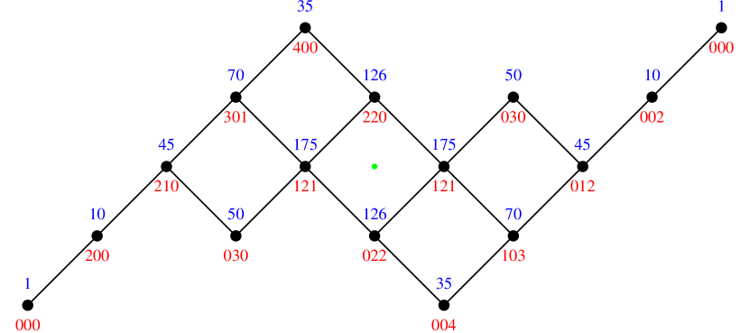
Figure 4. The ideal poset for $L_{4}=\operatorname{Sp}(4)/\operatorname{U}(4)$. The upper label on each node is the dimension of the corresponding subrepresentation of $\Lambda^{*,0}\bigl{(}\operatorname{\mathfrak{sp}}(4)/\operatorname{\mathfrak{u}}(4)\bigr{)}$ and the lower label is its highest weight as a representation of $\operatorname{SU}(4)$.

More detail about the topology and Schubert cell decomposition of $L_{m}$ can be found in [1]. Complete information about the irreducible constituents of the exterior powers of the cotangent bundle of $L_{m}$ and the consequent structure of its ideal poset is collected in a convenient form in [19]. The corresponding Hasse diagram for the case $m=4$ is drawn in Figure 4.

4.4.2. Ideals of degree $3$

I have not analyzed the boundary cases in all dimensions for the Lagrangian Grassmannian, so I will confine myself to studying the cases in the first interesting dimension, that of cycles of dimension or codimension equal to $3$.

The first task is to describe the irreducible decomposition of $\Lambda^{3,0}(\operatorname{\mathfrak{m}})$ under the action of $K=\operatorname{U}(m)$. Fortunately, this is relatively easy. Using the above description of the tangent bundle of $L_{m}$, one can see that, as a representation of $\operatorname{U}(n)$, the space $\operatorname{\mathfrak{m}}$ is isomorphic to the representation $S^{2}(\mathbb{C}^{\,m})={\mathbb{S}}_{(2)}(\mathbb{C}^{\,m})$ associated to the standard representation of $\operatorname{U}(m)$ on $\mathbb{C}^{\,m}$. Then a little work with multiplicity formulae from [9] shows that

(4.33) $$\Lambda^{3}\bigl{(}S^{2}(\mathbb{C}^{\,m})\bigr{)}\simeq\Lambda^{3}\bigl{(}{\mathbb{S}}_{(2)}(\mathbb{C}^{\,m})\bigr{)}\simeq{\mathbb{S}}_{(3,3)}(\mathbb{C}^{\,m})\oplus{\mathbb{S}}_{(4,1,1)}(\mathbb{C}^{\,m}).$$

These latter two representations are irreducible and their dimensions are given by [9, Theorem 6.3 or Exercise 6.4] as:

(4.34) $$\begin{split}\dim{\mathbb{S}}_{(3,3)}(\mathbb{C}^{\,m})&=\frac{m^{2}(m{+}1)^{2}(m{+}2)(m{-}1)}{144},\\ \dim{\mathbb{S}}_{(4,1,1)}(\mathbb{C}^{\,m})&=\frac{m(m^{2}{-}1)(m^{2}{-}4)(m{+}3)}{72}.\end{split}$$

Let ${\mathcal{I}}_{(3,3)}$ and ${\mathcal{I}}_{(4,1,1)}$, respectively, denote the exterior differential systems on $L_{m}$ generated in degree $3$ by the sections of ${\mathbb{S}}_{(3,3)}(S)\subset\Lambda^{3}(T^{*}L_{m})$ and ${\mathbb{S}}_{(4,1,1)}(S)\subset\Lambda^{3}(T^{*}L_{m})$.

4.4.3. Integral elements

The following linear algebra lemma identifies the integral elements of dimension three or more for each of the two $\operatorname{GL}(m,{\mathbb{C}})$-invariant subspaces of $\Lambda^{3}\bigl{(}S^{2}((\mathbb{C}^{\,m})^{*})\bigr{)}$.

Lemma 14.

Any subspace $E\subset S^{2}(\mathbb{C}^{\,m})$ of dimension $3$ or more on which all of the elements of ${\mathbb{S}}_{(3,3)}\bigl{(}(\mathbb{C}^{\,m})^{*}\bigr{)}$ vanish is of the form $E=L{\circ}W$ where $L\subset\mathbb{C}^{\,m}$ is a line and $W\subset\mathbb{C}^{\,m}$ is a subspace whose dimension is the same as that of $E$.

Any subspace $E\subset S^{2}(\mathbb{C}^{\,m})$ of dimension $3$ or more on which all of the elements of ${\mathbb{S}}_{(4,1,1)}\bigl{(}(\mathbb{C}^{\,m})^{*}\bigr{)}$ vanish must have dimension $3$ and be of the form $E=S^{2}(W)$ where $W\subset\mathbb{C}^{\,m}$ is a subspace of dimension $2$.

Proof.

This proof is very similar in spirit and structure to the proof of Lemma 13, so, to save space, I will not go into as much detail here as I did there. Instead, I will limit my discussion to the outline, except where some essentially new or different idea is needed.

Let $\eta:S^{2}(\mathbb{C}^{\,m})\to S^{2}(\mathbb{C}^{\,m})$ be the identity map. For any basis $\mathbf{v}_{1},\dots,\mathbf{v}_{m}$ of $\mathbb{C}^{\,m}$, write $\eta=\frac{1}{2}\eta^{ab}\mathbf{v}_{a}{\circ}\mathbf{v}_{b}$, where $\eta^{ab}=\eta^{ba}$ are 1-forms on $S^{2}(\mathbb{C}^{\,m})$. Note that $\{\eta^{ab}\mid a\leq b\}$ is a basis for the dual space.

Now, ${\mathbb{S}}_{(3,3)}(\mathbb{C}^{\,m})$ occurs as a constituent of $S^{3}(\mathbb{C}^{\,m})^{\otimes 2}$, but ${\mathbb{S}}_{(4,1,1)}(\mathbb{C}^{\,m})$ does not. Consequently, the $3$-forms of the form

(4.35) $$\psi(X,Y)=-\psi(Y,X)=X_{i_{1}i_{2}i_{3}}Y_{i_{4}i_{5}i_{6}}\,\eta^{i_{1}i_{2}}{\mathchoice{\,{\scriptstyle\wedge}\,}{{\scriptstyle\wedge}}{{\scriptscriptstyle\wedge}}{{\scriptscriptstyle\wedge}}}\eta^{i_{3}i_{4}}{\mathchoice{\,{\scriptstyle\wedge}\,}{{\scriptstyle\wedge}}{{\scriptscriptstyle\wedge}}{{\scriptscriptstyle\wedge}}}\eta^{i_{5}i_{6}}\,,$$

when $X$ and $Y$ are symmetric in their indices, must lie in the subspace ${\mathbb{S}}_{(3,3)}\bigl{(}(\mathbb{C}^{\,m})^{*}\bigr{)}$ of $\Lambda^{3}\bigl{(}S^{2}((\mathbb{C}^{\,m})^{*})\bigr{)}$. Taking, as a particular example, $X_{111}=Y_{222}=1$ and all other $X_{ijk}$, $Y_{ijk}$ equal to zero yields $\psi(X,Y)=\eta^{11}{\mathchoice{\,{\scriptstyle\wedge}\,}{{\scriptstyle\wedge}}{{\scriptscriptstyle\wedge}}{{\scriptscriptstyle\wedge}}}\eta^{12}{\mathchoice{\,{\scriptstyle\wedge}\,}{{\scriptstyle\wedge}}{{\scriptscriptstyle\wedge}}{{\scriptscriptstyle\wedge}}}\eta^{22}\not=0$, so the span of the $\psi(X,Y)$ is nontrivial. Since this span is invariant under $\operatorname{GL}(m,{\mathbb{C}})$ and since ${\mathbb{S}}_{(3,3)}\bigl{(}(\mathbb{C}^{\,m})^{*}\bigr{)}$ is irreducible, this span must be all of this subspace. Thus, ${\mathbb{S}}_{(3,3)}\bigl{(}(\mathbb{C}^{\,m})^{*}\bigr{)}$ is the span of the $3$-forms of the form (4.35).

Now, to begin, it must be checked that for every line $L\subset\mathbb{C}^{\,m}$, all of the forms $\psi(X,Y)$ vanish on the $m$-dimensional subspace $E=L{\circ}\mathbb{C}^{\,m}\subset S^{2}(\mathbb{C}^{\,m})$. By equivariance, it suffices to check this for the line $L=\mathbb{C}^{\,}{\cdot}\mathbf{v}_{1}$, which is defined by the equations $\eta^{ab}=0$ for $1<a\leq b$. Thus, the claim is equivalent to the claim that the forms $\psi(X,Y)$ all lie in the ideal generated by the $1$-forms $\eta^{ab}$ with $1<a\leq b$. By obvious reductions (keeping in mind that $\psi(X,Y)=-\psi(Y,X)$), it suffices to check this for the cases where $X_{11a}=X_{1a1}=X_{a11}=1$ but $X_{i_{1}i_{2}i_{3}}=0$ otherwise and $Y_{1bc}=Y_{1cb}=Y_{b1c}=Y_{c1b}=Y_{bc1}=Y_{cb1}=1$ but $Y_{i_{1}i_{2}i_{3}}=0$ otherwise. In this case, there are $9$ terms in the sum (4.35), and each term either vanishes identically, cancels in combination with one or two other terms, or else is a multiple of some $\eta^{pq}$ with $1<p\leq q$. Thus, the claim is established.

Now suppose that $E\subset S^{2}(\mathbb{C}^{\,m})$ is a subspace of dimension $d\geq 3$ on which all of the forms in ${\mathbb{S}}_{(3,3)}\bigl{(}(\mathbb{C}^{\,m})^{*}\bigr{)}$ vanish. The goal is to show that there is a unique line $L\subset\mathbb{C}^{\,m}$ so that $E\subset L{\circ}\mathbb{C}^{\,m}$. Let $\xi^{ab}$ be the restriction to $E$ of $\eta^{ab}$.

Now, $E$ will be defined by some set of linear relations among the $1$-forms $\xi^{ab}$. (By hypothesis, at least three of the $\xi^{ab}$ are linearly independent on $E$.) I need to show that one can choose the basis $\mathbf{v}_{1},\dots,\mathbf{v}_{m}$ so that these relations include $\xi^{ab}=0$ for $a,b>1$.

Suppose that the basis $\mathbf{v}_{1},\dots,\mathbf{v}_{m}$ has been chosen so that the maximum number, say $p$, of the forms $\xi^{11},\dots,\xi^{1m}$ are linearly independent. (This maximum independence will hold on a Zariski open set of bases $\mathbf{v}$.) Clearly, $1\leq p\leq\dim E$. It is not difficult to show that, by making a change of basis in $\mathbf{v}$, I can assume that $\xi^{11}{\mathchoice{\,{\scriptstyle\wedge}\,}{{\scriptstyle\wedge}}{{\scriptscriptstyle\wedge}}{{\scriptscriptstyle\wedge}}}\dots\mathchoice{\,{\scriptstyle\wedge}\,}{{\scriptstyle\wedge}}{{\scriptscriptstyle\wedge}}{{\scriptscriptstyle\wedge}}\xi^{1p}\not=0$ but that $\xi^{1a}=0$ for $a>p$. Then, by the same sort of analysis as was done in the proof of Lemma 13, one can show that maximality implies that

(4.36) $$\xi^{qr}\equiv 0\mod\xi^{11},\dots,\xi^{1p}\,,\qquad\qquad\text{when~{}$r>p$.}$$

Since the $\xi^{ab}$ must span $E^{*}$, the relations (4.36) imply that $p\geq 2$.

So far, no use has been made of the assumption that the forms in ${\mathbb{S}}_{(3,3)}\bigl{(}(\mathbb{C}^{\,m})^{*}\bigr{)}$ vanish on $E$, i.e., that

(4.37) $$0=X_{i_{1}i_{2}i_{3}}Y_{i_{4}i_{5}i_{6}}\,\xi^{i_{1}i_{2}}{\mathchoice{\,{\scriptstyle\wedge}\,}{{\scriptstyle\wedge}}{{\scriptscriptstyle\wedge}}{{\scriptscriptstyle\wedge}}}\xi^{i_{3}i_{4}}{\mathchoice{\,{\scriptstyle\wedge}\,}{{\scriptstyle\wedge}}{{\scriptscriptstyle\wedge}}{{\scriptscriptstyle\wedge}}}\xi^{i_{5}i_{6}}\,,$$

for all $X$ and $Y$ symmetric in their indices. To make any further progress, these relations will have to be used.

Since, as has already been seen, the relations (4.37) include $\xi^{11}{\mathchoice{\,{\scriptstyle\wedge}\,}{{\scriptstyle\wedge}}{{\scriptscriptstyle\wedge}}{{\scriptscriptstyle\wedge}}}\xi^{12}{\mathchoice{\,{\scriptstyle\wedge}\,}{{\scriptstyle\wedge}}{{\scriptscriptstyle\wedge}}{{\scriptscriptstyle\wedge}}}\xi^{22}=0$, it follows that $p\geq 3$. Now, replacing $2$ by $i\leq p$ in this relation gives $\xi^{11}{\mathchoice{\,{\scriptstyle\wedge}\,}{{\scriptstyle\wedge}}{{\scriptscriptstyle\wedge}}{{\scriptscriptstyle\wedge}}}\xi^{1i}{\mathchoice{\,{\scriptstyle\wedge}\,}{{\scriptstyle\wedge}}{{\scriptscriptstyle\wedge}}{{\scriptscriptstyle\wedge}}}\xi^{ii}=0$, so, in particular,

(4.38) $$\xi^{ii}\equiv 0\mod\xi^{11},\dots,\xi^{1p}.$$

On the other hand, polarizing the identity $\xi^{11}{\mathchoice{\,{\scriptstyle\wedge}\,}{{\scriptstyle\wedge}}{{\scriptscriptstyle\wedge}}{{\scriptscriptstyle\wedge}}}\xi^{1i}{\mathchoice{\,{\scriptstyle\wedge}\,}{{\scriptstyle\wedge}}{{\scriptscriptstyle\wedge}}{{\scriptscriptstyle\wedge}}}\xi^{ii}=0$ gives

(4.39) $$0=\xi^{11}{\mathchoice{\,{\scriptstyle\wedge}\,}{{\scriptstyle\wedge}}{{\scriptscriptstyle\wedge}}{{\scriptscriptstyle\wedge}}}\xi^{1i}{\mathchoice{\,{\scriptstyle\wedge}\,}{{\scriptstyle\wedge}}{{\scriptscriptstyle\wedge}}{{\scriptscriptstyle\wedge}}}\xi^{jk}+\xi^{11}{\mathchoice{\,{\scriptstyle\wedge}\,}{{\scriptstyle\wedge}}{{\scriptscriptstyle\wedge}}{{\scriptscriptstyle\wedge}}}\xi^{1j}{\mathchoice{\,{\scriptstyle\wedge}\,}{{\scriptstyle\wedge}}{{\scriptscriptstyle\wedge}}{{\scriptscriptstyle\wedge}}}\xi^{ki}+\xi^{11}{\mathchoice{\,{\scriptstyle\wedge}\,}{{\scriptstyle\wedge}}{{\scriptscriptstyle\wedge}}{{\scriptscriptstyle\wedge}}}\xi^{1k}{\mathchoice{\,{\scriptstyle\wedge}\,}{{\scriptstyle\wedge}}{{\scriptscriptstyle\wedge}}{{\scriptscriptstyle\wedge}}}\xi^{ij}\,$$

for all $2\leq i,j,k\leq p$. Since $p\geq 3$, taking any pair $(i,j)$ with $2\leq i<j\leq p$ and setting $k=j$ in the above relation yields

$$0=\xi^{11}{\mathchoice{\,{\scriptstyle\wedge}\,}{{\scriptstyle\wedge}}{{\scriptscriptstyle\wedge}}{{\scriptscriptstyle\wedge}}}\xi^{1i}{\mathchoice{\,{\scriptstyle\wedge}\,}{{\scriptstyle\wedge}}{{\scriptscriptstyle\wedge}}{{\scriptscriptstyle\wedge}}}\xi^{jj}+2\,\xi^{11}{\mathchoice{\,{\scriptstyle\wedge}\,}{{\scriptstyle\wedge}}{{\scriptscriptstyle\wedge}}{{\scriptscriptstyle\wedge}}}\xi^{1j}{\mathchoice{\,{\scriptstyle\wedge}\,}{{\scriptstyle\wedge}}{{\scriptscriptstyle\wedge}}{{\scriptscriptstyle\wedge}}}\xi^{ij}.$$

Wedging this relation with $\xi^{1i}$ gives $\xi^{11}{\mathchoice{\,{\scriptstyle\wedge}\,}{{\scriptstyle\wedge}}{{\scriptscriptstyle\wedge}}{{\scriptscriptstyle\wedge}}}\xi^{1i}{\mathchoice{\,{\scriptstyle\wedge}\,}{{\scriptstyle\wedge}}{{\scriptscriptstyle\wedge}}{{\scriptscriptstyle\wedge}}}\xi^{1j}{\mathchoice{\,{\scriptstyle\wedge}\,}{{\scriptstyle\wedge}}{{\scriptscriptstyle\wedge}}{{\scriptscriptstyle\wedge}}}\xi^{ij}=0$ whenever $2\leq i<j\leq p$. Since $\xi^{11}{\mathchoice{\,{\scriptstyle\wedge}\,}{{\scriptstyle\wedge}}{{\scriptscriptstyle\wedge}}{{\scriptscriptstyle\wedge}}}\xi^{1i}{\mathchoice{\,{\scriptstyle\wedge}\,}{{\scriptstyle\wedge}}{{\scriptscriptstyle\wedge}}{{\scriptscriptstyle\wedge}}}\xi^{1j}\not=0$ by hypothesis, it follows that

(4.40) $$\xi^{ij}\equiv 0\mod\xi^{11},\dots,\xi^{1p}.$$

It follows from (4.36), (4.38), and (4.40) that $\{\xi^{11},\dots,\xi^{1p}\}$ is a basis for $E^{*}$. Consequently, $p=d=\dim E$. Moreover, analysis of (4.39), shows that there must exist $S^{i}$ so that

$$\xi^{ij}\equiv S^{i}\,\xi^{1j}+S^{j}\,\xi^{1i}\mod\xi^{11},\qquad\qquad\text{for $2\leq i,j\leq d$}.$$

It follows that, by replacing $\mathbf{v}_{1}$ by $\mathbf{v}_{1}+S^{i}\,\mathbf{v}_{i}$, I can arrange that $\xi^{ij}\equiv 0\mod\xi^{11}$, so assume this.

Now, in the same way that (4.39) was derived, one can derive the relations

(4.41) $$0=\xi^{11}{\mathchoice{\,{\scriptstyle\wedge}\,}{{\scriptstyle\wedge}}{{\scriptscriptstyle\wedge}}{{\scriptscriptstyle\wedge}}}\xi^{1i}{\mathchoice{\,{\scriptstyle\wedge}\,}{{\scriptstyle\wedge}}{{\scriptscriptstyle\wedge}}{{\scriptscriptstyle\wedge}}}\xi^{jr}+\xi^{11}{\mathchoice{\,{\scriptstyle\wedge}\,}{{\scriptstyle\wedge}}{{\scriptscriptstyle\wedge}}{{\scriptscriptstyle\wedge}}}\xi^{1j}{\mathchoice{\,{\scriptstyle\wedge}\,}{{\scriptstyle\wedge}}{{\scriptscriptstyle\wedge}}{{\scriptscriptstyle\wedge}}}\xi^{ir},\qquad\text{when~{}$2\leq i,j\leq d<r$.}$$

and

(4.42) $$0=\xi^{11}{\mathchoice{\,{\scriptstyle\wedge}\,}{{\scriptstyle\wedge}}{{\scriptscriptstyle\wedge}}{{\scriptscriptstyle\wedge}}}\xi^{1i}{\mathchoice{\,{\scriptstyle\wedge}\,}{{\scriptstyle\wedge}}{{\scriptscriptstyle\wedge}}{{\scriptscriptstyle\wedge}}}\xi^{qr},\qquad\text{when~{}$2\leq i\leq d<q,r$.}$$

The relations (4.41) imply that there exist $A^{r}$ for $r>d$ so that $\xi^{jr}\equiv A^{r}\xi^{1j}\mod\xi^{11}$ when $2\leq j\leq d<r$, while (4.42) implies $\xi^{jr}\equiv 0\mod\xi^{11}$ when $d<q,r$. In particular, it follows that

$$\xi=\xi^{ab}\,\mathbf{v}_{a}\mathbf{v}_{b}\equiv 2\,\xi^{1i}\,(\mathbf{v}_{1}{+}A^{r}\mathbf{v}_{r}){\circ}\mathbf{v}_{i}\mod\xi^{11}.$$

Thus, the hyperplane $H=\ker\xi^{11}\subset E$ is of the form $H=L\circ W$ where the line $L\subset\mathbb{C}^{\,m}$ is spanned by the vector $\mathbf{v}_{1}^{\prime}=\mathbf{v}_{1}{+}A^{r}\mathbf{v}_{r}$ and $W$ is spanned by $\mathbf{v}_{2},\dots,\mathbf{v}_{d}$.

The analysis so far shows that every $E\subset S^{2}(\mathbb{C}^{\,m})$ of dimension $d\geq 3$ on which all the elements of ${\mathbb{S}}_{(3,3)}\bigl{(}(\mathbb{C}^{\,m})^{*}\bigr{)}$ vanish contains a hyperplane $H$ of the form $L{\circ}W$ where $L$ and $W$ are subspaces of $\mathbb{C}^{\,m}$ of dimensions $1$ and $d{-}1$, respectively, that are independent, i.e., $L\cap W=0$. To finish the characterization of these integral elements, it suffices to show that, for any basis $\mathbf{v}_{1},\dots,\mathbf{v}_{m}$, every integral element of ${\mathbb{S}}_{(3,3)}\bigl{(}(\mathbb{C}^{\,m})^{*}\bigr{)}$ that contains the $2$-plane spanned by $\mathbf{v}_{1}{\circ}\mathbf{v}_{2}$ and $\mathbf{v}_{1}{\circ}\mathbf{v}_{3}$ must be itself be a subspace of the $m$-plane $(\mathbb{C}^{\,}{\cdot}\mathbf{v}_{1}){\circ}\mathbb{C}^{\,m}$ (which has already been shown to be an integral element).

To see this, consider, for every $a,b>1$, the $3$-forms

$$\begin{split}\psi^{ab}&=\phantom{{}+{}}2\,\eta^{12}{\mathchoice{\,{\scriptstyle\wedge}\,}{{\scriptstyle\wedge}}{{\scriptscriptstyle\wedge}}{{\scriptscriptstyle\wedge}}}\eta^{13}{\mathchoice{\,{\scriptstyle\wedge}\,}{{\scriptstyle\wedge}}{{\scriptscriptstyle\wedge}}{{\scriptscriptstyle\wedge}}}\eta^{ab}+2\,\eta^{12}{\mathchoice{\,{\scriptstyle\wedge}\,}{{\scriptstyle\wedge}}{{\scriptscriptstyle\wedge}}{{\scriptscriptstyle\wedge}}}\eta^{1a}{\mathchoice{\,{\scriptstyle\wedge}\,}{{\scriptstyle\wedge}}{{\scriptscriptstyle\wedge}}{{\scriptscriptstyle\wedge}}}\eta^{b3}+2\,\eta^{12}{\mathchoice{\,{\scriptstyle\wedge}\,}{{\scriptstyle\wedge}}{{\scriptscriptstyle\wedge}}{{\scriptscriptstyle\wedge}}}\eta^{1b}{\mathchoice{\,{\scriptstyle\wedge}\,}{{\scriptstyle\wedge}}{{\scriptscriptstyle\wedge}}{{\scriptscriptstyle\wedge}}}\eta^{3a}\\ &\phantom{={}}+\phantom{2\,}\,\,\eta^{11}{\mathchoice{\,{\scriptstyle\wedge}\,}{{\scriptstyle\wedge}}{{\scriptscriptstyle\wedge}}{{\scriptscriptstyle\wedge}}}\eta^{23}{\mathchoice{\,{\scriptstyle\wedge}\,}{{\scriptstyle\wedge}}{{\scriptscriptstyle\wedge}}{{\scriptscriptstyle\wedge}}}\eta^{ab}+\phantom{2\,}\eta^{11}{\mathchoice{\,{\scriptstyle\wedge}\,}{{\scriptstyle\wedge}}{{\scriptscriptstyle\wedge}}{{\scriptscriptstyle\wedge}}}\eta^{2a}{\mathchoice{\,{\scriptstyle\wedge}\,}{{\scriptstyle\wedge}}{{\scriptscriptstyle\wedge}}{{\scriptscriptstyle\wedge}}}\eta^{b3}+\phantom{2\,}\eta^{11}{\mathchoice{\,{\scriptstyle\wedge}\,}{{\scriptstyle\wedge}}{{\scriptscriptstyle\wedge}}{{\scriptscriptstyle\wedge}}}\eta^{2b}{\mathchoice{\,{\scriptstyle\wedge}\,}{{\scriptstyle\wedge}}{{\scriptscriptstyle\wedge}}{{\scriptscriptstyle\wedge}}}\eta^{3a},\end{split}$$

which manifestly belong to ${\mathbb{S}}_{(3,3)}\bigl{(}(\mathbb{C}^{\,m})^{*}\bigr{)}$. When $a,b>3$,

$$\begin{split}\psi^{ab}\bigl{(}\mathbf{v}_{1}{\circ}\mathbf{v}_{2},\mathbf{v}_{1}{\circ}\mathbf{v}_{3},\mathbf{u}\bigr{)}&=2\,\eta^{ab}(\mathbf{u})\,,\\ \psi^{3b}\bigl{(}\mathbf{v}_{1}{\circ}\mathbf{v}_{2},\mathbf{v}_{1}{\circ}\mathbf{v}_{3},\mathbf{u}\bigr{)}&=4\,\eta^{3b}(\mathbf{u})\,,\\ \psi^{2b}\bigl{(}\mathbf{v}_{1}{\circ}\mathbf{v}_{2},\mathbf{v}_{1}{\circ}\mathbf{v}_{3},\mathbf{u}\bigr{)}&=2\,\eta^{2b}(\mathbf{u})\,,\end{split}$$

while

$$\begin{split}\psi^{33}\bigl{(}\mathbf{v}_{1}{\circ}\mathbf{v}_{2},\mathbf{v}_{1}{\circ}\mathbf{v}_{3},\mathbf{u}\bigr{)}&=6\,\eta^{33}(\mathbf{u})\,,\\ \psi^{23}\bigl{(}\mathbf{v}_{1}{\circ}\mathbf{v}_{2},\mathbf{v}_{1}{\circ}\mathbf{v}_{3},\mathbf{u}\bigr{)}&=4\,\eta^{23}(\mathbf{u})\,,\\ \psi^{22}\bigl{(}\mathbf{v}_{1}{\circ}\mathbf{v}_{2},\mathbf{v}_{1}{\circ}\mathbf{v}_{3},\mathbf{u}\bigr{)}&=2\,\eta^{22}(\mathbf{u})\,.\\ \end{split}$$

In particular, if $\{\mathbf{v}_{1}{\circ}\mathbf{v}_{2},\mathbf{v}_{1}{\circ}\mathbf{v}_{3},\mathbf{u}\}$ is to span an integral element of ${\mathbb{S}}_{(3,3)}\bigl{(}(\mathbb{C}^{\,m})^{*}\bigr{)}$, then $\eta^{ab}(\mathbf{u})=0$ when $a,b>1$, i.e., $\mathbf{u}$ must lie in the span of $\{\mathbf{v}_{1}{\circ}\mathbf{v}_{1},\dots,\mathbf{v}_{1}{\circ}\mathbf{v}_{m}\}$, i.e., $\mathbf{u}\in(\mathbb{C}^{\,}{\cdot}\mathbf{v}_{1}){\circ}\mathbb{C}^{\,m}$, which is what needed to be shown.

I now turn to the analysis of the integral elements of the ideal ${\mathcal{I}}_{(4,1,1)}$.

First, ${\mathbb{S}}_{(4,1,1)}(\mathbb{C}^{\,m})$ occurs as a constituent of $S^{3}(\mathbb{C}^{\,m})\otimes\Lambda^{3}(\mathbb{C}^{\,m})$, but ${\mathbb{S}}_{(3,3)}(\mathbb{C}^{\,m})$ does not. Consequently, the $3$-forms of the form

(4.43) $$\psi(X,Y)=X_{i_{1}i_{2}i_{3}}Y_{i_{4}i_{5}i_{6}}\,\eta^{i_{1}i_{4}}{\mathchoice{\,{\scriptstyle\wedge}\,}{{\scriptstyle\wedge}}{{\scriptscriptstyle\wedge}}{{\scriptscriptstyle\wedge}}}\eta^{i_{2}i_{5}}{\mathchoice{\,{\scriptstyle\wedge}\,}{{\scriptstyle\wedge}}{{\scriptscriptstyle\wedge}}{{\scriptscriptstyle\wedge}}}\eta^{i_{3}i_{6}}\,,$$

when $X$ is symmetric in its indices and $Y$ is skewsymmetric in its indices, must lie in the subspace ${\mathbb{S}}_{(4,1,1)}\bigl{(}(\mathbb{C}^{\,m})^{*}\bigr{)}$ of $\Lambda^{3}\bigl{(}S^{2}((\mathbb{C}^{\,m})^{*})\bigr{)}$. Taking, as a particular example, $X_{111}=1$ with all other $X_{ijk}$ equal to zero, and $Y_{123}=1$ but $Y_{ijk}=0$ unless $\{i,j,k\}=\{1,2,3\}$ yields $\psi(X,Y)=6\,\eta^{11}{\mathchoice{\,{\scriptstyle\wedge}\,}{{\scriptstyle\wedge}}{{\scriptscriptstyle\wedge}}{{\scriptscriptstyle\wedge}}}\eta^{12}{\mathchoice{\,{\scriptstyle\wedge}\,}{{\scriptstyle\wedge}}{{\scriptscriptstyle\wedge}}{{\scriptscriptstyle\wedge}}}\eta^{13}\not=0$. Thus, the span of the $\psi(X,Y)$ is nontrivial. Since this span is invariant under $\operatorname{GL}(m,{\mathbb{C}})$ and since ${\mathbb{S}}_{(4,1,1)}\bigl{(}(\mathbb{C}^{\,m})^{*}\bigr{)}$ is irreducible, this span must be all of this subspace. Thus, ${\mathbb{S}}_{(4,1,1)}\bigl{(}(\mathbb{C}^{\,m})^{*}\bigr{)}$ is the span of the $3$-forms of the form (4.43).

Now suppose that $E\subset S^{2}(\mathbb{C}^{\,m})$ is a subspace of dimension $d\geq 3$ on which all of the forms in ${\mathbb{S}}_{(4,1,1)}\bigl{(}(\mathbb{C}^{\,m})^{*}\bigr{)}$ vanish. The goal is to show that there is a $2$-plane $P\subset\mathbb{C}^{\,m}$ so that $E=S^{2}(P)$. Let $\xi^{ab}$ be the restriction to $E$ of $\eta^{ab}$.

Now, $E$ will be defined by some set of linear relations among the $1$-forms $\xi^{ab}$. (By hypothesis, at least three of the $\xi^{ab}$ are linearly independent on $E$.) I need to show that one can choose the basis $\mathbf{v}_{1},\dots,\mathbf{v}_{m}$ so that these relations include $\xi^{ab}=0$ when $b>2$.

Suppose that the basis $\mathbf{v}_{1},\dots,\mathbf{v}_{m}$ has been chosen so that the maximum number, say $p$, of the forms $\xi^{11},\dots,\xi^{1m}$ are linearly independent. (This maximum independence will hold on a Zariski open set of bases $\mathbf{v}$.) Clearly, $1\leq p\leq\dim E$. It is not difficult to show that, by making a change of basis in $\mathbf{v}$, I can assume that $\xi^{11}{\mathchoice{\,{\scriptstyle\wedge}\,}{{\scriptstyle\wedge}}{{\scriptscriptstyle\wedge}}{{\scriptscriptstyle\wedge}}}\dots\mathchoice{\,{\scriptstyle\wedge}\,}{{\scriptstyle\wedge}}{{\scriptscriptstyle\wedge}}{{\scriptscriptstyle\wedge}}\xi^{1p}\not=0$ but that $\xi^{1a}=0$ for $a>p$. Then, by the same sort of analysis as was done in the proof of Lemma 13, one can show that maximality of $p$ implies that

(4.44) $$\xi^{qr}\equiv 0\mod\xi^{11},\dots,\xi^{1p}\,,\qquad\qquad\text{when~{}$r>p$.}$$

Since the $\xi^{ab}$ must span $E^{*}$, the relations (4.44) imply that $p\geq 2$.

So far, no use has been made of the assumption that the forms in ${\mathbb{S}}_{(4,1,1)}\bigl{(}(\mathbb{C}^{\,m})^{*}\bigr{)}$ vanish on $E$, i.e., that

(4.45) $$0=X_{i_{1}i_{2}i_{3}}Y_{i_{4}i_{5}i_{6}}\,\xi^{i_{1}i_{4}}{\mathchoice{\,{\scriptstyle\wedge}\,}{{\scriptstyle\wedge}}{{\scriptscriptstyle\wedge}}{{\scriptscriptstyle\wedge}}}\xi^{i_{2}i_{5}}{\mathchoice{\,{\scriptstyle\wedge}\,}{{\scriptstyle\wedge}}{{\scriptscriptstyle\wedge}}{{\scriptscriptstyle\wedge}}}\xi^{i_{3}i_{6}}\,,$$

for all $X$ symmetric in its indices and $Y$ skewsymmetric in its indices. To make any further progress, these relations will have to be used.

Since, as has already been seen, the relations (4.45) include $\xi^{11}{\mathchoice{\,{\scriptstyle\wedge}\,}{{\scriptstyle\wedge}}{{\scriptscriptstyle\wedge}}{{\scriptscriptstyle\wedge}}}\xi^{12}{\mathchoice{\,{\scriptstyle\wedge}\,}{{\scriptstyle\wedge}}{{\scriptscriptstyle\wedge}}{{\scriptscriptstyle\wedge}}}\xi^{13}=0$, it follows that $p<3$, i.e., $p=2$. Moreover, since $p=2$, the relations (4.44) imply that $\{\xi^{11},\xi^{12},\xi^{22}\}$ must span $E^{*}$. Since $\dim E\geq 3$, by hypothesis, it follows that $\dim E=3$ and that $\bigl{(}\xi^{11},\xi^{12},\xi^{22}\bigr{)}$ must be a basis for $E^{*}$.

Now, fix $a>2$ and let $Y_{12a}=1$ with $Y_{ijk}=0$ unless $\{i,j,k\}=\{1,2,a\}$. Letting $X_{abc}$ be the general symmetric symbol with $X_{abc}=0$ unless $1\leq a,b,c\leq 2$, substituting this into the relations (4.45), and using the fact that $\xi^{1a}=0$ yields the relations

$$\xi^{11}{\mathchoice{\,{\scriptstyle\wedge}\,}{{\scriptstyle\wedge}}{{\scriptscriptstyle\wedge}}{{\scriptscriptstyle\wedge}}}\xi^{12}{\mathchoice{\,{\scriptstyle\wedge}\,}{{\scriptstyle\wedge}}{{\scriptscriptstyle\wedge}}{{\scriptscriptstyle\wedge}}}\xi^{2a}=\xi^{11}{\mathchoice{\,{\scriptstyle\wedge}\,}{{\scriptstyle\wedge}}{{\scriptscriptstyle\wedge}}{{\scriptscriptstyle\wedge}}}\xi^{22}{\mathchoice{\,{\scriptstyle\wedge}\,}{{\scriptstyle\wedge}}{{\scriptscriptstyle\wedge}}{{\scriptscriptstyle\wedge}}}\xi^{2a}=\xi^{12}{\mathchoice{\,{\scriptstyle\wedge}\,}{{\scriptstyle\wedge}}{{\scriptscriptstyle\wedge}}{{\scriptscriptstyle\wedge}}}\xi^{22}{\mathchoice{\,{\scriptstyle\wedge}\,}{{\scriptstyle\wedge}}{{\scriptscriptstyle\wedge}}{{\scriptscriptstyle\wedge}}}\xi^{2a}=0,$$

which implies $\xi^{2a}=0$. Now, fix $b>2$. Letting $X$ be the symmetric symbol that satisfies $X_{1,1,b}=1$ but $X_{ijk}=0$ unless $(i,j,k)$ is a permutation of $(1,1,b)$ gives the relation $\xi^{11}{\mathchoice{\,{\scriptstyle\wedge}\,}{{\scriptstyle\wedge}}{{\scriptscriptstyle\wedge}}{{\scriptscriptstyle\wedge}}}\xi^{12}{\mathchoice{\,{\scriptstyle\wedge}\,}{{\scriptstyle\wedge}}{{\scriptscriptstyle\wedge}}{{\scriptscriptstyle\wedge}}}\xi^{ab}=0$. Letting $X$ be the symmetric symbol that satisfies $X_{1,2,b}=1$ but $X_{ijk}=0$ unless $(i,j,k)$ is a permutation of $(1,2,b)$ gives the relation $\xi^{11}{\mathchoice{\,{\scriptstyle\wedge}\,}{{\scriptstyle\wedge}}{{\scriptscriptstyle\wedge}}{{\scriptscriptstyle\wedge}}}\xi^{22}{\mathchoice{\,{\scriptstyle\wedge}\,}{{\scriptstyle\wedge}}{{\scriptscriptstyle\wedge}}{{\scriptscriptstyle\wedge}}}\xi^{ab}=0$. Letting $X$ be the symmetric symbol that satisfies $X_{2,2,b}=1$ but $X_{ijk}=0$ unless $(i,j,k)$ is a permutation of $(2,2,b)$ gives the relation $\xi^{12}{\mathchoice{\,{\scriptstyle\wedge}\,}{{\scriptstyle\wedge}}{{\scriptscriptstyle\wedge}}{{\scriptscriptstyle\wedge}}}\xi^{22}{\mathchoice{\,{\scriptstyle\wedge}\,}{{\scriptstyle\wedge}}{{\scriptscriptstyle\wedge}}{{\scriptscriptstyle\wedge}}}\xi^{ab}=0$. These three identities imply that $\xi^{ab}=0$ when $a,b>2$, which is what remained to be shown. ∎

Remark 43 (Integral element orbit structure).

Note an interesting feature of the above description of the integral elements of ${\mathbb{S}}_{(3,3)}\bigl{(}(\mathbb{C}^{\,m})^{*}\bigr{)}$ when $m>3$: The space of integral elements of a given dimension $d$ in the range $3\leq d<m$ is not homogeneous under the action of $\operatorname{GL}(m,{\mathbb{C}})$. After all, such integral elements are of the form $L{\circ}W$ where $L$ and $W$ are subspaces of $\mathbb{C}^{\,m}$ of dimensions $1$ and $d$, respectively. Generically, one will have $L\cap W=0$ and this describes a $\operatorname{GL}(m,{\mathbb{C}})$-orbit that is open and dense in the space of $d$-dimensional integral elements. However, there are ‘special’ integral elements that satisfy $L\subset W$, and these constitute a closed $\operatorname{GL}(m,{\mathbb{C}})$-orbit of their own.

4.4.4. Integral varieties

The next two propositions describe the integral manifolds of the exterior differential systems ${\mathcal{I}}_{(3,3)}$ and ${\mathcal{I}}_{(4,1,1)}$. I remind the reader that $m\geq 3$ throughout this subsection.

Before stating the first of these two propositions, I need to describe a family of subvarieties of $L_{m}$.

Example 22 (A Lagrangian Schubert cycle).

If $P\subset\mathbb{C}^{\,2m}$ is any sub-Lagrangian $(m{-}1)$-plane, it lies in a $1$-parameter family of Lagrangian $m$-planes:

$$[P,\mathbb{C}^{\,2m}]_{m}\cap L_{m}\simeq{\mathbb{P}}^{1}.$$

Let $S\subset\mathbb{C}^{\,2m}$ be any Lagrangian $m$-plane, and define a closed subvariety $\sigma(S)\subset L_{m}$ by

$$\sigma(S)=\{\ V\in L_{m}\ \mid\ \dim(V\cap S)\geq m{-}1\ \}.$$

Of course $S$ lies in $\sigma(S)$, and there is a natural submersion

$$\kappa:\sigma(S)\setminus\{S\}\to\operatorname{Gr}(m{-}1,S)\simeq{\mathbb{P}}(S^{*})\simeq{\mathbb{P}}^{m-1}$$

defined by $\kappa(V)=S\cap V$ when $V\in\sigma(S)$ is not $S$ itself. By the first statement in this example, the fibers of $\kappa$ are biholomorphic to ${\mathbb{C}}$. It follows that $\sigma(S)$ is an irreducible subvariety of $L_{m}$ of dimension $m$ and that $\sigma(S)$ is smooth away from $S$.

It is not difficult to see that the tangent cone to $\sigma(S)$ at $S\in L_{m}$ is the cone consisting of the quadratic forms in $T_{S}L_{m}\simeq S^{2}(S^{*})$ that are perfect squares. Thus, $S$ is a genuine singular point of $\sigma(S)$.

Proposition 11.

For $S\in L_{m}$, the variety $\sigma(S)$ is an integral of ${\mathcal{I}}_{(3,3)}$.

Conversely, if $X\subset L_{m}$ is an irreducible variety of dimension at least $3$ that is an integral of ${\mathcal{I}}_{(3,3)}$, then there is an $S\in L_{m}$ so that $X\subset\sigma(S)$.

Proof.

The first task (which will be needed in the next proposition as well), is to establish the equations of the moving frame for submanifolds of $L_{m}$.

Define $\operatorname{Sp}(m,{\mathbb{C}})$ be the subgroup of $\operatorname{SL}(2m,{\mathbb{C}})$ consisting of the matrices $\mathsf{v}$ that satisfy

(4.46) $${}^{t}\mathsf{v}\begin{pmatrix}0_{m}&-\operatorname{I}_{m}\\ \operatorname{I}_{m}&0_{m}\end{pmatrix}\mathsf{v}=\begin{pmatrix}0_{m}&-\operatorname{I}_{m}\\ \operatorname{I}_{m}&0_{m}\end{pmatrix}.$$

I will regard $\mathsf{v}:\operatorname{Sp}(m,{\mathbb{C}})\to\operatorname{GL}(2m,{\mathbb{C}})$ as a matrix-valued function and denote its columns as

$$\mathsf{v}=(\mathsf{v}_{1}\quad\dots\quad\mathsf{v}_{m}\quad\mathsf{v}^{1}\quad\dots\quad\mathsf{v}^{m})$$

where $\mathsf{v}_{i},\mathsf{v}^{i}:\operatorname{Sp}(m,{\mathbb{C}})\to\mathbb{C}^{\,2m}$ are regarded as (holomorphic) mappings.

Define

$$\pi(\mathsf{v})=[\mathsf{v}_{1}{\mathchoice{\,{\scriptstyle\wedge}\,}{{\scriptstyle\wedge}}{{\scriptscriptstyle\wedge}}{{\scriptscriptstyle\wedge}}}\dots\mathchoice{\,{\scriptstyle\wedge}\,}{{\scriptstyle\wedge}}{{\scriptscriptstyle\wedge}}{{\scriptscriptstyle\wedge}}\mathsf{v}_{m}]\,,$$

so that $\pi$ is a surjective submersion $\pi:\operatorname{Sp}(m,{\mathbb{C}})\to L_{m}$. The fibers of $\pi$ are the orbits of the parabolic subgroup $P\subset\operatorname{Sp}(m,{\mathbb{C}})$ consisting of elements of the form

(4.47) $$\mathsf{v}=\begin{pmatrix}A&AB\\ 0_{m}&{}^{t}\!A^{-1}\end{pmatrix}\qquad\text{for~{}$A\in\operatorname{GL}(m,{\mathbb{C}})$ and~{}$B={}^{t}\!B\in\mathbb{C}^{\,m,m}$.}$$

Thus, $\pi:\operatorname{Sp}(m,{\mathbb{C}})\to L_{m}$ is a principal right $P$-bundle over $L_{m}$.

In accordance with the usual moving frame conventions, write the structure equations as

(4.48) $$\mathrm{d}\mathsf{v}=\mathrm{d}(\mathsf{v}_{i}\ \mathsf{v}^{i})=(\mathsf{v}_{j}\ \mathsf{v}^{j})\begin{pmatrix}\alpha^{j}_{i}&\gamma^{ji}\\ \beta_{ji}&-\alpha^{i}_{j}\end{pmatrix}=\mathsf{v}\,\theta$$

where

(4.49) $$\beta_{ji}=\beta_{ij}\quad\text{and}\quad\gamma^{ji}=\gamma^{ij}\,,$$

but the components of $\alpha$, $\beta$, and $\gamma$ are otherwise linearly independent. The relations (4.49) follow in the usual way from the exterior derivative of (4.46). The structure equation $\mathrm{d}\theta=-\theta{\mathchoice{\,{\scriptstyle\wedge}\,}{{\scriptstyle\wedge}}{{\scriptscriptstyle\wedge}}{{\scriptscriptstyle\wedge}}}\theta$ holds since $\theta=\mathsf{v}^{-1}\,\mathrm{d}\mathsf{v}$. These expand to

(4.50) $$\begin{split}\mathrm{d}\alpha^{i}_{j}&=-\alpha^{i}_{k}{\mathchoice{\,{\scriptstyle\wedge}\,}{{\scriptstyle\wedge}}{{\scriptscriptstyle\wedge}}{{\scriptscriptstyle\wedge}}}\alpha^{k}_{j}-\gamma^{ik}{\mathchoice{\,{\scriptstyle\wedge}\,}{{\scriptstyle\wedge}}{{\scriptscriptstyle\wedge}}{{\scriptscriptstyle\wedge}}}\beta_{kj}\,,\\ \mathrm{d}\beta_{ij}&=-\beta_{ik}{\mathchoice{\,{\scriptstyle\wedge}\,}{{\scriptstyle\wedge}}{{\scriptscriptstyle\wedge}}{{\scriptscriptstyle\wedge}}}\alpha^{k}_{j}+\alpha^{k}_{i}{\mathchoice{\,{\scriptstyle\wedge}\,}{{\scriptstyle\wedge}}{{\scriptscriptstyle\wedge}}{{\scriptscriptstyle\wedge}}}\beta_{kj}\,,\\ \mathrm{d}\gamma^{ij}&=-\alpha^{i}_{k}{\mathchoice{\,{\scriptstyle\wedge}\,}{{\scriptstyle\wedge}}{{\scriptscriptstyle\wedge}}{{\scriptscriptstyle\wedge}}}\gamma^{kj}+\gamma^{ik}{\mathchoice{\,{\scriptstyle\wedge}\,}{{\scriptstyle\wedge}}{{\scriptscriptstyle\wedge}}{{\scriptscriptstyle\wedge}}}\alpha^{j}_{k}\,.\end{split}$$

Now suppose that $X\subset L_{m}$ is an irreducible integral variety of ${\mathcal{I}}_{(3,3)}$ of dimension $d\geq 3$, and let $X^{\circ}\subset X$ denote its smooth locus, which is an embedded submanifold of $L_{m}$. For every $V\in X^{\circ}$, the tangent space $T_{V}X$ is an integral element of ${\mathcal{I}}_{(3,3)}$ of dimension $d\geq 3$. By Lemma 14, there is a Zariski-open subset $X^{\diamond}\subset X^{\circ}$ (which may be empty) that consists of the elements $V\in X^{\circ}$ such that $T_{V}X=L_{V}\circ W_{V}$ where $L_{V}$ and $W_{V}$ are subspaces of $V^{*}$ of dimensions $1$ and $d$, respectively, and $L_{V}\cap W_{V}=0$. (See Remark 43.) The proof has to be broken up into two cases now, depending on whether or not $X^{\diamond}$ is empty. (Note that $X^{\diamond}$ cannot be empty unless $d<m$.)

The first case is that $X^{\diamond}$ is not empty, so assume this. Note that $X^{\diamond}$ is connected since $X$ is irreducible. Now, for every $V\in X^{\diamond}$, there exists a $\mathsf{v}\in\operatorname{Sp}(m,{\mathbb{C}})$ so that

1. $V$ is spanned by $\mathsf{v}_{1},\dots,\mathsf{v}_{m}$, and

2. $T_{V}X$ is spanned by $[\![\mathsf{v}^{1}]\!]{\circ}[\![\mathsf{v}^{2}]\!],[\![\mathsf{v}^{1}]\!]{\circ}[\![\mathsf{v}^{3}]\!],\dots,[\![\mathsf{v}^{1}]\!]{\circ}[\![\mathsf{v}^{d+1}]\!]$.

Let $F(X^{\diamond})\subset\operatorname{Sp}(m,{\mathbb{C}})$ denote the set of such $\mathsf{v}$ as $V$ ranges over $X^{\diamond}$. Then $\pi:F(X^{\diamond})\to X^{\diamond}$ is a principal $G$-bundle over $X^{\diamond}$, where $G\subset P$ is a subgroup of the matrices of the form (4.47) with ${}^{t}\!A^{-1}$ in $P_{1}\cap P_{d+1}\subset\operatorname{GL}(m,{\mathbb{C}})$. The reader can write out the exact conditions defining $G$ and verify that it is connected.

By construction, the forms $\beta_{12},\dots,\beta_{1(d{+}1)}$ are linearly independent on $F(X^{\diamond})$ and span the $\pi$-semibasic $1$-forms, while $\beta_{11}=\beta^{ab}=0$ when either $b>d{+}1$ or $a$ and $b$ are both greater than $1$.

This paragraph of the argument is necessary only if $d{+}1<m$, so suppose this is so for the moment. Choose a pair $(i,a)$ satisfying $2\leq i\leq d{+}1<a\leq m$ and differentiate the relation $\beta_{ia}=0$. By the structure equations, this is

$$0=\mathrm{d}\beta_{ia}=-\beta_{i1}{\mathchoice{\,{\scriptstyle\wedge}\,}{{\scriptstyle\wedge}}{{\scriptscriptstyle\wedge}}{{\scriptscriptstyle\wedge}}}\alpha^{1}_{a}\,.$$

Since $d\geq 3$, and since $\beta_{12},\dots,\beta_{1(d{+}1)}$ are linearly independent, $\alpha^{1}_{a}=0$ for $a>d{+}1$.

Now choose a pair $(i,j)$ with $2\leq i,j\leq d{+}1$ and differentiate $\beta_{ij}=0$. The structure equations give that

$$0=\mathrm{d}\beta_{ij}=-\beta_{i1}{\mathchoice{\,{\scriptstyle\wedge}\,}{{\scriptstyle\wedge}}{{\scriptscriptstyle\wedge}}{{\scriptscriptstyle\wedge}}}\alpha^{1}_{j}+\alpha^{1}_{i}{\mathchoice{\,{\scriptstyle\wedge}\,}{{\scriptstyle\wedge}}{{\scriptscriptstyle\wedge}}{{\scriptscriptstyle\wedge}}}\beta_{1j}\,.$$

Equivalently,

(4.51) $$\alpha^{1}_{i}{\mathchoice{\,{\scriptstyle\wedge}\,}{{\scriptstyle\wedge}}{{\scriptscriptstyle\wedge}}{{\scriptscriptstyle\wedge}}}\beta_{1j}+\alpha^{1}_{j}{\mathchoice{\,{\scriptstyle\wedge}\,}{{\scriptstyle\wedge}}{{\scriptscriptstyle\wedge}}{{\scriptscriptstyle\wedge}}}\beta_{1i}=0$$

This relation implies that there exists a function $\lambda$ on $F(X^{\diamond})$ so that $\alpha^{1}_{i}=\lambda\,\beta_{i}$ for $2\leq i\leq d{+}1$.

Computing how the function $\lambda$ varies on the fibers of $\pi$ (a standard computation in the technique of the moving frame) shows that the equation $\lambda=0$ defines a principal right $G_{1}$-bundle $F_{1}\subset F(X^{\diamond})$ over $X^{\diamond}$ where $G_{1}\subset G$ is a certain connected Lie subgroup of codimension $1$.

Since the previous paragraph showed that $\alpha^{1}_{a}=0$ for all $a>d{+}1$, it now follows that the identities $\alpha^{1}_{i}=0$ for all $i>1$ hold on $F_{1}$. This vanishing together with the fact that $\beta_{ij}=0$ for all $i,j\geq 2$ yield the congruences

$$\mathrm{d}\mathsf{v}_{2}\equiv\dots\equiv\mathrm{d}\mathsf{v}_{m}\equiv\mathrm{d}\mathsf{v}^{1}\equiv 0\mod\mathsf{v}_{2}\,,\dots,\mathsf{v}_{m}\,,\mathsf{v}^{1}\,.$$

In other words, the mapping $\nu:F_{1}\to L_{m}$ defined by $\nu(\mathsf{v})=[\mathsf{v}_{2}{\mathchoice{\,{\scriptstyle\wedge}\,}{{\scriptstyle\wedge}}{{\scriptscriptstyle\wedge}}{{\scriptscriptstyle\wedge}}}\dots\mathchoice{\,{\scriptstyle\wedge}\,}{{\scriptstyle\wedge}}{{\scriptscriptstyle\wedge}}{{\scriptscriptstyle\wedge}}\mathsf{v}_{m}{\mathchoice{\,{\scriptstyle\wedge}\,}{{\scriptstyle\wedge}}{{\scriptscriptstyle\wedge}}{{\scriptscriptstyle\wedge}}}\mathsf{v}^{1}]$ is locally constant and hence, by connectedness, globally constant. Let $S\in L_{m}$ be $m$-plane that is the image of $\nu$. Of course, it now follows that $S\cap\pi(\mathsf{v})$ is the $(m{-}1)$-plane $[\mathsf{v}_{2}{\mathchoice{\,{\scriptstyle\wedge}\,}{{\scriptstyle\wedge}}{{\scriptscriptstyle\wedge}}{{\scriptscriptstyle\wedge}}}\dots\mathchoice{\,{\scriptstyle\wedge}\,}{{\scriptstyle\wedge}}{{\scriptscriptstyle\wedge}}{{\scriptscriptstyle\wedge}}\mathsf{v}_{m}]$. Thus, $X^{\diamond}=\pi(F_{1})$ lies in $\sigma(S)$. Of course, this implies that $X$ itself lies in $\sigma(S)$ as well, as desired.

Now, consider the second case, in which $X^{\diamond}=\emptyset$. Then for every $V\in X^{\circ}$, the tangent space $T_{V}X$ is of the form $L_{V}\circ W_{V}$ where $L_{V}$ and $W_{V}$ are subspaces of $V^{*}$ of dimensions $1$ and $d$, respectively, and $L_{V}\subset W_{V}$. (Again, see Remark 43.) Note that $X^{\circ}$ is connected since $X$ is irreducible. For every $V\in X^{\circ}$, there exists a $\mathsf{v}\in\operatorname{Sp}(m,{\mathbb{C}})$ so that

1. $V$ is spanned by $\mathsf{v}_{1},\dots,\mathsf{v}_{m}$, and

2. $T_{V}X$ is spanned by $[\![\mathsf{v}^{1}]\!]{\circ}[\![\mathsf{v}^{1}]\!],[\![\mathsf{v}^{1}]\!]{\circ}[\![\mathsf{v}^{2}]\!],\dots,[\![\mathsf{v}^{1}]\!]{\circ}[\![\mathsf{v}^{d}]\!]$.

Let $F(X^{\circ})\subset\operatorname{Sp}(m,{\mathbb{C}})$ denote the set of such $\mathsf{v}$ as $V$ ranges over $X^{\circ}$. Then $\pi:F(X^{\circ})\to X^{\circ}$ is a principal $G$-bundle over $X^{\circ}$, where $G\subset P$ is the group consisting of the matrices of the form (4.47) with ${}^{t}\!A^{-1}$ in $P_{1}\cap P_{d}\subset\operatorname{GL}(m,{\mathbb{C}})$.

By construction, the forms $\beta_{11},\dots,\beta_{1d}$ are linearly independent on $F(X^{\circ})$ and span the $\pi$-semibasic $1$-forms, while $\beta^{ab}=0$ when either $b>d$ or $a$ and $b$ are both greater than $1$.

This paragraph of the argument is necessary only if $d<m$, so suppose this is so for the moment. Choose a pair $(i,a)$ satisfying $2\leq i\leq d<a\leq m$ and differentiate the relation $\beta_{ia}=0$. By the structure equations, this is

$$0=\mathrm{d}\beta_{ia}=-\beta_{i1}{\mathchoice{\,{\scriptstyle\wedge}\,}{{\scriptstyle\wedge}}{{\scriptscriptstyle\wedge}}{{\scriptscriptstyle\wedge}}}\alpha^{1}_{a}\,.$$

Since $d\geq 3$, and since $\beta_{12},\dots,\beta_{1d}$ are linearly independent, $\alpha^{1}_{a}=0$ for $a>d$.

Now choose a pair $(i,j)$ with $2\leq i,j\leq d$ and differentiate $\beta_{ij}=0$. The structure equations give

$$0=\mathrm{d}\beta_{ij}=-\beta_{i1}{\mathchoice{\,{\scriptstyle\wedge}\,}{{\scriptstyle\wedge}}{{\scriptscriptstyle\wedge}}{{\scriptscriptstyle\wedge}}}\alpha^{1}_{j}+\alpha^{1}_{i}{\mathchoice{\,{\scriptstyle\wedge}\,}{{\scriptstyle\wedge}}{{\scriptscriptstyle\wedge}}{{\scriptscriptstyle\wedge}}}\beta_{1j}\,.$$

Equivalently,

(4.52) $$\alpha^{1}_{i}{\mathchoice{\,{\scriptstyle\wedge}\,}{{\scriptstyle\wedge}}{{\scriptscriptstyle\wedge}}{{\scriptscriptstyle\wedge}}}\beta_{1j}+\alpha^{1}_{j}{\mathchoice{\,{\scriptstyle\wedge}\,}{{\scriptstyle\wedge}}{{\scriptscriptstyle\wedge}}{{\scriptscriptstyle\wedge}}}\beta_{1i}=0$$

This relation implies that there exists a function $\lambda$ on $F(X^{\circ})$ so that $\alpha^{1}_{i}=\lambda\,\beta_{i}$ for $2\leq i\leq d$.

Computing how the function $\lambda$ varies on the fibers of $\pi$ (a standard computation in the technique of the moving frame) shows that the equation $\lambda=0$ defines a principal right $G_{1}$-bundle $F_{1}\subset F(X^{\circ})$ over $X^{\circ}$ where $G_{1}\subset G$ is a certain connected Lie subgroup of codimension $1$.

Since the previous paragraph showed that $\alpha^{1}_{a}=0$ for all $a>d$, it now follows that the identities $\alpha^{1}_{i}=0$ for all $i>1$ hold on $F_{1}$. This vanishing together with the fact that $\beta_{ij}=0$ for all $i,j\geq 2$ yield the congruences

$$\mathrm{d}\mathsf{v}_{2}\equiv\dots\equiv\mathrm{d}\mathsf{v}_{m}\equiv\mathrm{d}\mathsf{v}^{1}\equiv 0\mod\mathsf{v}_{2}\,,\dots,\mathsf{v}_{m}\,,\mathsf{v}^{1}\,.$$

In other words, the mapping $\nu:F_{1}\to L_{m}$ defined by $\nu(\mathsf{v})=[\mathsf{v}_{2}{\mathchoice{\,{\scriptstyle\wedge}\,}{{\scriptstyle\wedge}}{{\scriptscriptstyle\wedge}}{{\scriptscriptstyle\wedge}}}\dots\mathchoice{\,{\scriptstyle\wedge}\,}{{\scriptstyle\wedge}}{{\scriptscriptstyle\wedge}}{{\scriptscriptstyle\wedge}}\mathsf{v}_{m}{\mathchoice{\,{\scriptstyle\wedge}\,}{{\scriptstyle\wedge}}{{\scriptscriptstyle\wedge}}{{\scriptscriptstyle\wedge}}}\mathsf{v}^{1}]$ is locally constant and hence, by connectedness, globally constant. Let $S\in L_{m}$ be $m$-plane that is the image of $\nu$. Of course, it now follows that $S\cap\pi(\mathsf{v})$ is the $(m{-}1)$-plane $[\mathsf{v}_{2}{\mathchoice{\,{\scriptstyle\wedge}\,}{{\scriptstyle\wedge}}{{\scriptscriptstyle\wedge}}{{\scriptscriptstyle\wedge}}}\dots\mathchoice{\,{\scriptstyle\wedge}\,}{{\scriptstyle\wedge}}{{\scriptscriptstyle\wedge}}{{\scriptscriptstyle\wedge}}\mathsf{v}_{m}]$. Thus, $X^{\circ}=\pi(F_{1})$ lies in $\sigma(S)$. Of course, this implies that $X$ itself lies in $\sigma(S)$ as well, as desired.

That $\sigma(S)$ really is an integral variety of ${\mathcal{I}}_{(3,3)}$ follows immediately from the argument in the second case (with $d=m$). ∎

By Lemma 14, there are no integral manifolds of ${\mathcal{I}}_{(4,1,1)}$ of dimension greater than $3$. The following proposition classifies the $3$-dimensional integral varieties of ${\mathcal{I}}_{(4,1,1)}$.

First, a definition. For any sub-Lagrangian subspace $A\subset\mathbb{C}^{\,2m}$, let $L_{m}(A)\subset L_{m}$ denote the set of $P\in L_{m}$ that contain $A$. Note that, if $a=\dim A<m$, then $L_{m}(A)$ is a smooth subvariety of $L_{m}$ that is isomorphic to $L_{m-a}$.

Proposition 12.

Let $X\subset L_{m}$ be an irreducible variety of dimension $3$ that is an integral variety of ${\mathcal{I}}_{(4,1,1)}$. Then there is a sub-Lagrangian $(m{-}2)$-plane $A\subset\mathbb{C}^{\,2m}$ so that $X\subset L_{m}(A)$.

Thus, if $X$ is closed, then $X=L_{m}(A)\simeq L_{2}\simeq Q_{3}$.

Proof.

Recall the moving frame notation and constructions from the first part of the proof of Proposition 11.

Suppose now that $X\subset L_{m}$ is an irreducible $3$-dimensional integral variety of of ${\mathcal{I}}_{(4,1,1)}$ and let $X^{\circ}\subset X$ be its smooth locus, which is connected since $X$ is irreducible. By Lemma 14, for every $V\in X^{\circ}$, there exists a $\mathsf{v}\in\operatorname{Sp}(m,{\mathbb{C}})$ so that

1. $V$ is spanned by $\mathsf{v}_{1},\dots,\mathsf{v}_{m}$, and

2. The tangent space $T_{V}X^{\circ}$ is spanned by $[\![\mathsf{v}^{1}]\!]{\circ}[\![\mathsf{v}^{1}]\!],\>[\![\mathsf{v}^{1}]\!]{\circ}[\![\mathsf{v}^{2}]\!],\>[\![\mathsf{v}^{2}]\!]{\circ}[\![\mathsf{v}^{2}]\!]$.

Let $F(X^{\circ})\subset\operatorname{Sp}(m,{\mathbb{C}})$ denote the set of such $\mathsf{v}$ as $V$ ranges over $X^{\circ}$. Then $\pi:F(X^{\circ})\to X^{\circ}$ is a principal right $G$-bundle over $X^{\circ}$ where $G\subset P$ is the subgroup consisting of the matrices of the form (4.47) with ${}^{t}\!A^{-1}$ in $P_{3}\subset\operatorname{GL}(m,{\mathbb{C}})$. Since $G$ and $X^{\circ}$ are each connected, it follows that $F(X^{\circ})$ is also connected.

By construction, the $1$-forms $\beta_{11},\beta_{12},\beta_{22}$ are linearly independent on $F(X^{\circ})$ and span the $\pi$-semibasic $1$-forms, while $\beta_{ij}=0$ if either $i$ or $j$ is greater than $2$.

Let $i>2$ be fixed and differentiate the identities $\beta_{i1}=\beta_{i2}=0$ using the structure equations. The result is equations of the form

$$\begin{pmatrix}\alpha^{1}_{i}&\alpha^{2}_{i}\end{pmatrix}{\mathchoice{\,{\scriptstyle\wedge}\,}{{\scriptstyle\wedge}}{{\scriptscriptstyle\wedge}}{{\scriptscriptstyle\wedge}}}\begin{pmatrix}\beta_{11}&\beta_{12}\\ \beta_{12}&\beta_{22}\end{pmatrix}=\begin{pmatrix}0&0\end{pmatrix}.$$

By the linear independence of $\beta_{11},\beta_{12},\beta_{22}$, it follows that $\alpha^{1}_{i}=\alpha^{2}_{i}=0$.

This vanishing for all $i>2$ implies

$$\mathrm{d}\mathsf{v}_{3}\equiv\dots\equiv\mathrm{d}\mathsf{v}_{m}\equiv 0\mod\mathsf{v}_{3},\dots,\mathsf{v}_{m}\,,$$

i.e., the $(m{-}2)$-plane $[\mathsf{v}_{3}{\mathchoice{\,{\scriptstyle\wedge}\,}{{\scriptstyle\wedge}}{{\scriptscriptstyle\wedge}}{{\scriptscriptstyle\wedge}}}\dots\mathsf{v}_{m}]$ is locally constant on $F(X^{\circ})$. Since $F(X^{\circ})$ is connected, this map must be constant. Thus, let $A\in\operatorname{Gr}(m{-}3,2m)$ be the isotropic plane so that $[\mathsf{v}_{3}{\mathchoice{\,{\scriptstyle\wedge}\,}{{\scriptstyle\wedge}}{{\scriptscriptstyle\wedge}}{{\scriptscriptstyle\wedge}}}\dots\mathsf{v}_{m}]\equiv A$. By construction, $A\subset V$ for all $V\in X^{\circ}$, so it follows that $X^{\circ}$ and, hence, $X$ are subsets of $L_{m}(A)$, as desired. ∎

These propositions allow characterizations of the extremal classes in $H_{6}(L_{m})$ that are analogous to that of Schubert cycles in Grassmannians:

Theorem 18.

Let $A\subset\mathbb{C}^{\,2m}$ be a sub-Lagrangian plane of dimension $m{-}2$. Fix a Lagrangian $m$-plane $S\subset\mathbb{C}^{\,2m}$ and let $B\subset S$ be a subspace of dimension $m{-}3$. Define two $3$-dimensional subvarieties of $L_{m}$ by

(4.53) $$X=\sigma(S)\cap[B,\mathbb{C}^{\,2m}]_{m}\qquad\text{and}\qquad Y=L_{m}(A).$$

Then $[X]$ and $[Y]$ are the generators of $H^{+}_{6}(L_{m},{\mathbb{Z}})\simeq{\mathbb{Z}}^{2}$.

An irreducible $Z\in{\mathcal{Z}}^{+}_{3}(L_{m})$ satisfies $[Z]=r[X]$ for some $r>0$ if and only if it lies in $\sigma(T)$ for some $T\in L_{m}$.

An irreducible $Z\in{\mathcal{Z}}^{+}_{3}(L_{m})$ satisfies $[Z]=r[Y]$ if and only if $r=1$ and $Z=L_{m}(D)$ for some isotropic $D\subset\mathbb{C}^{\,2m}$ of dimension $m{-}2$.

Proof.

First of all, it follows by either [2] or (4.33) and the general results of Kostant mentioned above that $b_{6}(L_{m})=2$. Let $\phi_{1}$ be the $\operatorname{SO}(2m)$-invariant Kähler form on $L_{m}$ whose cohomology class is a generator of $H^{2}(L_{m},{\mathbb{Z}})$. By (4.5), there is a sum of the form

$${\phi_{1}}^{3}=\mu^{(3,3)}\,\phi_{(3,3)}+\mu^{(4,1,1)}\,\phi_{(4,1,1)}$$

where $\mu^{(3,3)}>0$ and $\mu^{(4,1,1)}>0$ and $\phi_{(3,3)}$ and $\phi_{(4,1,1)}$ are positive $\operatorname{SO}(2m)$-invariant forms that are dual to the generalized Schubert cycles $\sigma_{(3,3)^{*}}$ and $\sigma_{(4,1,1)^{*}}$ of complex dimension $3$ whose cohomology classes generate $H^{+}_{6}(L_{m})$.

It follows that $\sigma_{(3,3)^{*}}$ is an irreducible $3$-dimensional integral of ${\mathcal{I}}_{(4,1,1)}$ and so, by Proposition 12, must be of the form $L_{m}(C)$ for some isotropic $m{-}3$ plane $C$. Thus $\sigma_{(3,3)^{*}}$ is homologous to $Y$.

It also follows that $\sigma_{(4,1,1)^{*}}$ is an irreducible $3$-dimensional integral of ${\mathcal{I}}_{(3,3)}$, and so, by Proposition 11, must lie in $\sigma(T)$ for some $T\in L_{m}$. When $m=3$, the dimension of $\sigma(T)$ is $3$, so $\sigma_{(4,1,1)^{*}}$ must be equal to $\sigma(T)$, which is $X$ in this case. The definition of $X$ now makes it clear that $X$ represents $\sigma_{(4,1,1)^{*}}$ when $m>3$ as well.

Finally, if $Z\in{\mathcal{Z}}^{+}_{3}(L_{m})$ is irreducible and satisfies $[Z]=r[X]$, then the integral of $\phi_{(3,3)}$ over $Z$ must be zero, so $\phi_{(3,3)}$ must vanish on $Z$. Thus $Z$ is an integral manifold of ${\mathcal{I}}_{(3,3)}$ and Proposition 11 applies.

The argument when $[Z]=r[Y]$ is similar. ∎

The extremal cycles of codimension $3$ in $L_{m}$ also display rigidity. I am not going to give all the details of this discussion, since most of the methods of proof in each of the two cases I am going to consider will, by now, be familiar to the reader. Instead, I will simply mention the points at which some interesting or different idea comes into play.

Theorem 19.

Let $Y\subset{\mathbb{P}}^{2m-1}$ be a subvariety of dimension $m{-}3$ and degree $r$. Let $\Psi(Y)\subset L_{m}$ denote the set of $V\in L_{m}$ satisfying ${\mathbb{P}}(V)\cap Y\not=\emptyset$.

Then $\Psi(Y)$ has codimension $3$ in $L_{m}$ and satisfies $\bigl{[}\Psi(Y)\bigr{]}=r\bigl{[}\sigma_{(4,1,1)}\bigr{]}$.

Moreover, any codimension $3$ subvariety $X\subset L_{m}$ that satisfies $[X]=r\bigl{[}\sigma_{(4,1,1)}\bigr{]}$ is $\Psi(Y)$ for some subvariety $Y\subset{\mathbb{P}}^{2m-1}$ of dimension $m{-}3$ and degree $r$.

Proof.

The analysis is very similar to that for the proof of Theorem 17, so I will leave the details to the reader. Only one aspect of the proof requires comment: Since there are two types of integral elements of ${\mathcal{I}}_{(3,3)}$, there are, correspondingly, two types of integral elements of ${\mathcal{I}}_{(3,3)^{*}}$. This forces a subdivision into two cases like that of Proposition 11, but this offers no essential new difficulty. ∎

Remark 44.

It is not difficult to see that $\Psi(Y)$ is always singular when $m\geq 4$. Thus, the homology classes of the form $r\bigl{[}\sigma_{(4,1,1)}\bigr{]}$ cannot be represented by smooth, effective cycles when $m\geq 4$.

Theorem 20.

Let $P\subset\mathbb{C}^{\,2m}$ be a Lagrangian $m$-plane and let

$$\Sigma(P)=\left\{\ V\in L_{m}\mid\dim(V\cap P)\geq 2\ \right\}.$$

Then $\Sigma(P)$ is of codimension $3$ in $L_{m}$ and represents the Schubert cycle $\sigma_{(3,3)}$.

Any irreducible variety $X\subset L_{m}$ of codimension $3$ that satisfies $[X]=r\,\bigl{[}\Sigma(P)\bigr{]}$ is of the form $X=\Sigma(Q)$ for some Lagrangian $m$-plane $Q$.

Proof.

Follow the pattern of the proof of Theorem 16. ∎

Remark 45 (Singularity of $\Sigma(P)$).

The variety $\Sigma(P)$ is singular when $m\geq 3$. In fact, $P$ itself is a singular point of $\Sigma(P)$, as is easily verified. In particular, Theorem 20 implies that, when $m\geq 3$, no multiple of the homology class $[\sigma_{(3,3)}]$ can be represented by a smooth, effective cycle.

4.5. The space E III

I have not done any deep analysis of the ideals on the Hermitian symmetric space $\mathsf{E\,III}=\operatorname{E}_{6}/\bigl{(}S^{1}{\cdot}\operatorname{Spin}(10)\bigr{)}$ (which has (complex) dimension $16$), but in this section, I will indicate some of the interesting possibilities that are turned up by a preliminary analysis.

Using a program such as simpLie, it is not difficult to compute the poset of ideals of $\mathsf{E\,III}$. The Hasse diagram for this poset is drawn in Figure 5.

I have not attempted to label the nodes, partly through lack of space. However, it will be convenient to be able to refer to some of the nodes, so I will do so by coordinates. Thus, the left-most node in the figure has coordinates $(0,0)$ and they continue upwards and to the right as $(1,1)$, $(2,2)$, $(3,3)$, with the first case of two nodes at the same level being at level $4$, namely $(4,4)$ and $(4,2)$. The lowest central node is $(8,0)$, and so on. I will refer to the corresponding ideals on $\mathsf{E\,III}$ by ${\mathcal{I}}_{(p,q)}$. Thus, for example, ${\mathcal{I}}_{(p,q)}$ is generated in degree $p$ and the first interesting ideals are ${\mathcal{I}}_{(4,2)}$ and ${\mathcal{I}}_{(4,4)}$. In this notation, $\bigl{|}(p,q)\bigr{|}=p$ and $(p,q)^{*}=(16{-}p,q)$.

Figure 5. The ideal poset for $\mathsf{E\,III}=\operatorname{E}_{6}/\bigl{(}S^{1}{\cdot}\operatorname{Spin}(10)\bigr{)}$.

These nodes could also be labeled by the the highest weight of the corresponding irreducible subrepresentation of $\Lambda^{*}(\operatorname{\mathfrak{m}})$, where $\operatorname{\mathfrak{m}}=\operatorname{\mathfrak{e}}_{6}/\bigl{(}\operatorname{\mathfrak{t}}{+}\operatorname{\mathfrak{so}}(10)\bigr{)}$, with respect to a maximal torus in $K=S^{1}{\cdot}\operatorname{Spin}(10)$. It is traditional to do this by labeling the nodes of the Dynkin diagram of $K$ with the coordinates of the highest weight, so I will do this in a compactified form. Thus, the summand $\Lambda^{1}(\operatorname{\mathfrak{m}})=\operatorname{\mathfrak{m}}$, which is, of course, irreducible and of dimension $16$, will be notated as $1{\cdot}$$\scriptstyle 000^{\scriptstyle 1}_{\scriptstyle 0}$. It corresponds to the node $(1,1)$.

The node $(4,2)$ is the representation $4{\cdot}$$\scriptstyle 020^{\scriptstyle 0}_{\scriptstyle 0}$ of dimension $770$, which is considerably smaller than the node $(4,4)$, the representation $4{\cdot}$$\scriptstyle 100^{\scriptstyle 0}_{\scriptstyle 2}$ of dimension $1050$. Thus, one might expect the integrals of the ideal ${\mathcal{I}}_{(4,2)}$ to display more flexibility than those of ${\mathcal{I}}_{(4,4)}$. In fact, as the Hasse diagram makes clear, ${\mathcal{I}}_{(4,4)}$ contains all forms of degree $5$ or higher, so its maximal integrals have dimension $4$. It would be interesting to know whether or not all its irreducible integral varieties are the obvious Schubert varieties of dimension $4$. In contrast, the ideal ${\mathcal{I}}_{(4,2)}$ has integrals of dimension at least $5$, since the corresponding form $\phi_{(4,2)}$ vanishes on the $5$-dimensional Schubert cycles that correspond to the node $(5,5)$.

In fact, the node $(5,5)$ is very interesting, corresponding to the representation $5{\cdot}$$\scriptstyle 000^{\scriptstyle 0}_{\scriptstyle 3}$ of dimension $672$, which is less than 20% of the size of its ‘competitor’ at level $5$, namely the node $(5,3)$ which is the representation $5{\cdot}$$\scriptstyle 110^{\scriptstyle 0}_{\scriptstyle 1}$ of dimension $3696$. Again, note that the ideal ${\mathcal{I}}_{(5,3)}$ contains all $6$-forms, so that its maximal integrals are $5$-dimensional. Meanwhile, the ideal ${\mathcal{I}}_{(5,5)}$ fails to contain forms of degree as high as $8$. It would be interesting to know whether the maximal dimension irreducible integrals of this ideal are the $8$-dimensional Schubert cycles that correspond to the node $(8,0)$.

As a final note on size disparity among the ideals, the node $(8,0)$ corresponds to the representation $8{\cdot}$$\scriptstyle 400^{\scriptstyle 0}_{\scriptstyle 0}$ whose dimension is $660$, a remarkably small number in comparison with the dimensions associated to the nearby nodes. One might expect the integrals of the ideal ${\mathcal{I}}_{(8,0)}$ to be particularly interesting. For example, could it be the case that every irreducible integral of ${\mathcal{I}}_{(8,0)}$ of dimension at least $8$ lies in one of the $11$-dimensional Schubert varieties associated to the node $(11,5)$? (It is evident that these Schubert varieties are integrals of ${\mathcal{I}}_{(8,0)}$ and that this ideal has no integrals of dimension greater than $11$.)

The exploration of these problems is postponed to a later date.

4.6. The space E VII

I have not done any deep analysis of the ideals on the Hermitian symmetric space $\mathsf{E\,VII}=\operatorname{E}_{7}/\bigl{(}S^{1}{\cdot}\operatorname{E}_{6}\bigr{)}$ (which has (complex) dimension $27$), but in this section, I will indicate some of the interesting possibilities that are turned up by a preliminary analysis.

Using a program such as simpLie, it is not difficult to compute the poset of ideals of $\mathsf{E\,VII}$. The Hasse diagram for this poset is drawn in Figure 6.

I have not attempted to label the nodes, partly through lack of space. However, it will be convenient to be able to refer to some of the nodes, so I will do so by coordinates. Thus, the left-most node in the figure has coordinates $(0,0)$ and they continue upwards and to the right as $(1,1)$, $(2,2)$, $(3,3)$, with the first case of two nodes at the same level being at level $5$, namely $(5,5)$ and $(5,3)$. For each node $(p,q)$, I will refer to the corresponding ideal on $\mathsf{E\,VII}$ by ${\mathcal{I}}_{(p,q)}$. Thus, for example, ${\mathcal{I}}_{(p,q)}$ is generated in degree $p$ and the first interesting ideals are ${\mathcal{I}}_{(5,3)}$ and ${\mathcal{I}}_{(5,5)}$. In this notation, $\bigl{|}(p,q)\bigr{|}=p$ and $(p,q)^{*}=(27{-}p,8{-}q)$.

Figure 6. The ideal poset for $\mathsf{E\,VII}=\operatorname{E}_{7}/\bigl{(}S^{1}{\cdot}\operatorname{E}_{6}\bigr{)}$.

These nodes could also be labeled by the the highest weight of the corresponding irreducible subrepresentation of $\Lambda^{*}(\operatorname{\mathfrak{m}})$, where $\operatorname{\mathfrak{m}}=\operatorname{\mathfrak{e}}_{7}/\bigl{(}\operatorname{\mathfrak{t}}{+}\operatorname{\mathfrak{e}}_{6}\bigr{)}$, with respect to a maximal torus in $K=S^{1}{\cdot}\operatorname{E}_{6}$. It is traditional to do this by labeling the nodes of the Dynkin diagram of $K$ with the coordinates of the highest weight, so I will do this in a compactified form. Thus, the summand $\Lambda^{1}(\operatorname{\mathfrak{m}})=\operatorname{\mathfrak{m}}$, which is, of course, irreducible and of dimension $27$, will be notated as $1{\cdot}\begin{smallmatrix}&&0\\ 1&0&0&0&0\end{smallmatrix}$. It corresponds to the node $(1,1)$.

The figure makes clear some of the interesting features of the ideals, so I will not belabor them here, except to mention two of the more interesting nodes:

The node $(6,6)$ is the representation  $6{\cdot}\begin{smallmatrix}&&3\\ 0&0&0&0&0\end{smallmatrix}$ of dimension $43,758$, which is only slightly more than one-eighth of the dimension of the representation associated to its ‘competitor’ node $(6,4)$. Note also that ${\mathcal{I}}_{(6,6)}$ has irreducible integrals of dimension $10$, namely the Schubert cycles corresponding to the node $(10,0)$. It would be interesting to know whether any irreducible integral of ${\mathcal{I}}_{(6,6)}$ of dimension $6$ or more is a subvariety of one of these $10$-dimensional Schubert cycles.

The node $(10,0)$ is the representation  $10{\cdot}\begin{smallmatrix}&&0\\ 0&0&0&0&5\end{smallmatrix}$ of dimension $100,386$, which is less than one-eightieth of the dimension of $\Lambda^{10}(\operatorname{\mathfrak{m}})$. Note also that ${\mathcal{I}}_{(10,0)}$ has irreducible integrals of dimension $17$, namely the Schubert cycles corresponding to the node $(17,8)$. It would be interesting to know whether any irreducible integral of ${\mathcal{I}}_{(10,0)}$ of dimension $10$ or more is a subvariety of one of these $17$-dimensional Schubert cycles.

Again, answers to these questions will have to await a detailed study of the ideals involved.

References

- [1] I. M. Bernšteĭn, I. Gel′fand, and S. Gel′fand, Schubert cells and the cohomology of the spaces , (Russian) Uspehi Mat. Nauk 28 (1973), 3–26. (Also available in English translation: Russian Math. Surveys 28 (1973), 1–26.) MR 55:2941
- [2] A. Borel and F. Hirzebruch, Characteristic classes and homogeneous spaces, I, Amer. J. Math. 80 (1958), 458–538. MR 21:1586
- [3] R. Bryant, S.-S. Chern, R. Gardner, H. Goldschmidt, and P. Griffiths, Exterior Differential Systems, Springer-Verlag, New York, 1991. MR 92h:58007
- [4] É. Cartan, Sur la structure des groupes de transformations finis et continus, Thèse, Paris, Nony, 1894.
- [5] A. Cassa, The topology of the space of positive analytic cycles, Ann. Mat. Pura Appl. (4) 112 (1977), 1–12. MR 56:662
- [6] C. Ehresmann, Sur la topologie de certains espaces homogènes, Ann. of Math. 35 (1934), 396–443.
- [7] G. Fano, Studio di alcuni sistemi di rette considerati come superficie dello spazio a cinque dimensioni, Annali di Matematica (2) 21 (1893), 141–192.
- [8] W. Fulton and R. Lazarsfeld, Positive polynomials for ample vector bundles, Ann. of Math. (2) 118 (1983), 35–60. MR 85e:14021
- [9] W. Fulton and J. Harris, Representation Theory, Graduate Texts in Mathematics, no. 129, Springer-Verlag, New York, 1991. MR 93a:20069
- [10] P. Griffiths, Hermitian differential geometry, Chern classes, and positive vector bundles, in D. Spencer and S. Iyanaga (eds.) Global Analysis Princeton Math. Series No. 29, Tokyo (1969), 185–251. MR 41:2717
- [11] P. Griffiths and J. Harris, Principles of Algebraic Geometry, Wiley Interscience, John Wiley & Sons, New York, 1978. (For Grassmannians, see esp. Chapter 1, Sect.5. For Chern classes, see esp. Chapter 3, Sect.3.) MR 80b:14001
- [12] P. Griffiths and J. Harris, Algebraic geometry and local differential geometry, Ann. Sci. École Norm. Sup. (4) 12, 1979, 355–452. MR 81k:53004
- [13] R. Hartshorne, Algebraic Geometry, Graduate Texts in Mathematics 52, Springer-Verlag, Berlin, 1977. MR 57:3116
- [14] R. Hartshorne, E. Rees, and E. Thomas, Nonsmoothing of algebraic cycles on Grassmann varieties, Bull. Amer. Math. Soc. 80 (1974), 847–851. MR 50:9870
- [15] F. R. Harvey and A. W. Knapp, Positive forms, Wirtinger’s inequality and currents, in Value Distribution Theory, Part A, eds. R. O. Kujala and A. L. Vitter, Marcel Dekker, Inc., New York, 1974. 43–62. MR 50:7573
- [16] S. Helgason, Differential Geometry, Lie Groups, and Symmetric Spaces, Academic Press, New York, 1978. MR 80k:53081
- [17] B. Kostant, Lie algebra cohomology and the generalized Borel-Weil theorem, Ann. Math 74 (1961), 329–387. MR 26:265
- [18] B. Kostant, Lie algebra cohomology and generalized Schubert cells, Ann. Math 77 (1963), 72–144. MR 26:266
- [19] K. Künnemann and H. Tamvakis, The Hodge star operator on Schubert forms, preprint, October, 1999.
- [20] V. Lakshmibai and S.S. Sheshadri, Singular locus of a Schubert variety, Bull. Amer. Math. Soc. (N.S.) 11 (1984), 363–366. MR 85j:14095
- [21] D. Lieberman, Compactness of the Chow scheme: applications to automorphisms and deformations of Kähler manifolds, in Fonctions de plusieurs variables complexes, III (Sém. François Norguet, 1975–1977), Springer, Berlin, 1978, 140–186. MR 80h:32056
- [22] S. Lojasiewicz, Triangulation of semi-analytic sets, Ann. Scuol. Norm. di Pisa 18 (1964), 449-474. MR 30:3478
- [23] J. Milnor and J. Stasheff, Characteristic Classes, Annals of Mathematics Studies, no. 76, Princeton University Press, Princeton, 1974. MR 55:13428
- [24] W. Stoll, Invariant forms on Grassmann manifolds, Annals of Mathematics Studies, no. 89, Princeton University Press, Princeton, 1977. MR 58:1235
- [25] R. Thom, Sous-variétés et classes d’homologie des variétés différentiables, I & II, C. R. Acad. Sci. Paris 236 (1953), 453–454, 573–575. MR 14:1005a MR 14:1005b
- [26] R. Thom, Quelques propriétés globales des variétés différentiables, Comment. Math. Helv. 28 (1954), 17–86. MR 15:890a
- [27] M. Walters, Geometry and uniqueness of some extreme subvarieties in complex Grassmannians, Ph.D. thesis, University of Michigan, 1997.
- [28] M. Walters, Uniqueness of some extreme -dimensional subvarieties of , preprint, 1998.
- [29] M. Walters, Rigidity of some solutions to Schubert differential systems over , preprint, 1998.