The Gromov–Witten invariants of symplectic toric manifolds

Résumé

We study the fix point components of the big torus action on the moduli space of stable maps into a smooth projective toric variety, and apply Graber and Pandharipande’s localization formula for the virtual fundamental class to obtain an explicit formula

for the Gromov–Witten invariants of toric varieties. Using this formula we compute all genus–$0$ $3$–point invariants of the Fano manifold ${\mathbb{P}}({\mathcal{O}}_{{\mathbb{P}}^{2}}(2)\oplus 1)$, and we show for the (non–Fano) manifold ${\mathbb{P}}({\mathcal{O}}_{{\mathbb{P}}^{2}}(3)\oplus 1)$ that its quantum cohomology ring does not correspond to Batyrev’s ring defined in [Bat93].

Nous étudions les composantes des points fixes de l’action du gros tore sur l’espace de modules des applications stables dans une variété torique projective lisse. En appliquant la formule de localisation de Graber et Pandharipande à la classe fondamentale virtuelle de l’espace de modules, nous obtenons une formule explicite pour les invariants de Gromov–Witten des variétés toriques. À l’aide de cette nouvelle formule, nous calculons tous les invariants de genre 0 à trois points de la variété de Fano ${\mathbb{P}}({\mathcal{O}}_{{\mathbb{P}}^{2}}(2)\oplus 1)$ et montrons que pour la variété ${\mathbb{P}}({\mathcal{O}}_{{\mathbb{P}}^{2}}(3)\oplus 1)$, qui n’est pas de Fano, l’anneau de la cohomologie quantique ne correspond pas à l’anneau défini par Batyrev dans [Bat93].

1. Introduction

The aim of this article is to give a formula that computes the Gromov–Witten invariants of symplectic toric manifolds.

Gromov–Witten invariants

Gromov–Witten invariants and quantum cohomology express essentially the same symplecto–topological data first studied by Witten in theoretical physics ([Wit91]). In fact, he looked at quantum cohomology as an example of a topological $\sigma$–model where what we now call Gromov–Witten invariants are basically the correlation functions. This lead to the interpretation of these invariants as counting certain (pseudo–)holomorphic curves in a symplectic manifold.

Let $(M,\omega)$ be a compact symplectic manifold, and $J$ be a compatible almost–complex structure on $(M,\omega)$. A map $f:(\Sigma_{g},j)\longrightarrow(M,J)$ from a genus–$g$ curve $(\Sigma_{g},j)$ to $M$ is called $J$–holomorphic if $f$ is ${\mathbb{C}}$–linear, namely if

$$\bar{\partial}_{J}f:=\frac{1}{2}(df+J\circ df\circ j)=0.$$

For Kähler manifolds $(M,\omega,J)$, these are exactly the holomorphic maps. Now we fix an integral degree–$2$ homology class $A\in H_{2}(M,{\mathbb{Z}})$, and only look at $J$–holomorphic maps such that $f_{*}[\Sigma_{g}]=A$. For some classes $A$, there will be only a finite number of such curves up to reparametrization, and this number will be, under certain genericity assumptions, one of the Gromov–Witten invariants of the manifold $(M,\omega)$.

This number, though, is not a priori a symplectic invariant: the construction above strongly depends on the chosen compatible almost–complex structure $J$. In fact, even the dimension of the space of $J$–holomorphic maps $f:(\Sigma_{g},j)\longrightarrow(M,J)$ with $f_{*}[\Sigma_{g}]=A$ might change for different almost–complex structures $J$, that is, the above number might be defined for some $J$, but not for some others. This phenomenon of a “moduli space of $J$–holomorphic maps” being too big comes from the unpleasant property of the $\bar{\partial}_{J}$–operator of not always being transversal to the zero section in the infinite dimensional vector bundle

$$\mathcal{E}\mathrel{\smash{\mathop{\hbox to28.45274pt{\rightarrowfill}}}}\operatorname{Map}(\Sigma_{g},M)$$

whose fiber at $f\in\operatorname{Map}(\Sigma_{g},M)$ is the space $\mathcal{E}_{f}=\Omega^{0,1}(f^{*}TM)$. In fact, $\bar{\partial}_{J}$ is a Fredholm operator, and its index can be computed using Riemann–Roch arguments. We will usually refer to this index as the virtual dimension of the corresponding moduli space, since the index is equal to the actual dimension of the moduli space when $\bar{\partial}_{J}$ is indeed transversal (to the above mentioned zero section). Note that being a Fredholm operator in particular includes the property of the index being finite.

There is, however, another important problem of such a “definition” of an invariant: the moduli space of $J$–holomorphic curves in a degree–$2$ homology class $A$ is in general not compact. Take for example the family of conics that is given by the equation $xy=\varepsilon$. For $\varepsilon>0$, these conics are all smooth, but in the limit $\varepsilon\longrightarrow 0$ we obtain a singular conic with a node. In fact, Gromov has proven in [Gro85] that this is all that can happen: a series of $J$–holomorphic maps converges to a $J$–holomorphic map with singularities at worst nodes, i.e. where the underlying curve $\Sigma_{g}$ might have nodes. So to compactify the moduli space of $J$–holomorphic curves it suffices to add these curves with nodes, an approach that eventually lead to Kontsevich’s space of stable maps. This strategy, though, has one big disadvantage: the dimensions of the boundary components that we have to add for this compactification can be bigger than the dimension of the moduli space we started with, even the virtual dimension of the boundary components might get bigger. So we might end up counting $J$–holomorphic curves with nodes instead of smooth curves.

In the past years, the above mentioned difficulties have been resolved by different means, keeping more or less the intuitive idea of the invariant counting certain curves. Ruan and Tian ([RT95]) were the first who rigorously defined Gromov–Witten invariants in a mathematical context. They restricted themselves to weakly monotone symplectic manifolds. These manifolds have the nice property that the virtual dimension of the boundary components is always smaller than the virtual dimension of the moduli space of smooth curves. Moreover, they were able to show that for a generic almost–complex structure $J$, the operator $\bar{\partial}_{J}$ is transversal for all components of the compactified moduli space. So, in the case of weakly monotone symplectic manifolds, the invariant still counts $J$–holomorphic curves. However, the description of all $J$–holomorphic curves in a symplectic manifold for an arbitrary almost–complex structure $J$ (compatible with the symplectic structure) remains an unsolved problem.

Later, several successful attempts were undertaken to define Gromov–Witten invariants for all symplectic manifolds (for example [Sie96, LT98c, FO99]), as well as for projective complex varieties (for example [BF97, LT98b]). All constructions in both categories of varieties follow basically the same principle: instead of trying to obtain a moduli space of the expected dimension with a fundamental class, they take any compatible (respectively the given) almost–complex structure $J$ and construct a virtual fundamental class in the moduli space corresponding to $J$. The virtual fundamental class so defined is then supposed to behave as the fundamental class of a generic moduli space (if it existed at all).

Although the constructions in both categories are technically quite different, the Gromov–Witten invariants obtained are the same (see [Sie98, LT98a]). Actually, even the main idea for the construction of the virtual fundamental class is the same in both approaches: they both use excess intersection theory to “slice out” a cycle in exactly the right dimension, being led by the observation that the operator $\bar{\partial}_{J}$ is not transversal. In the algebro–geometric construction this is done by using a particular tangent obstruction theory $E^{\bullet}$, that is a two–term complex of locally free sheaves on the moduli space $\mathcal{M}$ and a morphism (in the derived category)

$$\phi:E^{\bullet}\mathrel{\smash{\mathop{\hbox to28.45274pt{\rightarrowfill}}}}L_{\mathcal{M}}^{\bullet}$$

to the cotangent complex $L^{\bullet}_{\mathcal{M}}$ of the moduli space, such that the rank $\operatorname{rk}E^{\bullet}=\operatorname{rk}(E^{0}-E^{-1})$ of the complex $E^{\bullet}$ is constant and equal to the virtual dimension of the moduli space $\mathcal{M}$. Roughly speaking, one can say that this obstruction theory $\phi:E^{\bullet}\longrightarrow L_{\mathcal{M}}^{\bullet}$ encodes how the virtual moduli cycle has to be cut out off the moduli space $\mathcal{M}$.

The above mentioned equivalence of the definitions in the two different categories opens an interesting opportunity for manifolds that are symplectic and complex varieties at the same time, Kähler manifolds: one could try to use the rather developed machinery of algebraic geometry to finally obtain symplectic invariants!

Toric manifolds

Toric manifolds, i.e. those which contain an algebraic torus as an open and dense subset and whose action on itself extends to the entire manifold, are an important set of examples to consider here because many are in fact Kähler. Moreover, although they include representatives of many classes of manifolds so far looked at in the context of Gromov–Witten invariants (complex projective space; Fano and weakly monotone manifolds), most toric manifolds do not fit into any of these groups. In spite of this diversity, all toric manifolds are combinatorically classified with the help of fans that basically describe the intersection pattern of the divisors of the toric variety.

However, what makes toric manifolds particularly nice to us is the action of the “big” torus on them. This action has only finitely many stable submanifolds which again can be easily derived from the fan description of the toric manifold. In addition, the action on the toric manifold $X$ naturally induces a torus action on the moduli spaces of stable maps to $X$, the fixed point components of which can be described combinatorically in terms of the zero and one dimensional stable submanifolds in $X$, hence again by fan data. This opens to us the possibility to apply equivariant theory to our problem.

Equivariant theory

In [GP99] Graber and Pandharipande have proven a localization formula for algebraic stacks $Y$ with a ${\mathbb{C}}^{*}$–action and a ${\mathbb{C}}^{*}$–equivariant perfect obstruction theory that can be ${\mathbb{C}}^{*}$–equivariantly embedded into a non–singular Deligne–Mumford stack. Similarly to the classical localization formula, they look, on a fixed point component $Y_{i}$ of the action on the stack $Y$, at a decomposition of the obstruction theory $E_{i}^{\bullet}$ restricted to $Y_{i}$ into the part that is fixed by the action, and the moving part:

$$E_{i}^{\bullet}=E_{i}^{\bullet,{\text{fix}}}\oplus E_{i}^{\bullet,{\text{move}}}.$$

Their main observation is that the fixed part $E_{i}^{\bullet,{\text{fix}}}$ is again an obstruction theory for the fixed point component $Y_{i}$, and that the role of the normal bundle is taken by the moving part $E^{\bullet,{\text{move}}}$, accordingly called virtual normal bundle: $N_{i}^{\text{vir}}=E_{i,\bullet}^{\text{move}}$, where $E_{i,\bullet}$ is the dual complex to $E^{\bullet}_{i}$.

To be precise, let $Y$ be an algebraic stack with a ${\mathbb{C}}^{*}$–action that can be ${\mathbb{C}}^{*}$–equivariantly embedded into a non-singular Deligne–Mumford stack. Let $\phi:E^{\bullet}\rightarrow L^{\bullet}_{Y}$ be a ${\mathbb{C}}^{*}$–equivariant perfect obstruction theory for $Y$, $[Y,E^{\bullet}]$ and $[Y_{i},E_{i}^{\bullet}]$ be the virtual fundamental classes of $Y$ and $E^{\bullet}$, and of the fixed point components $Y_{i}$ and the induced perfect obstruction theories $E_{i}^{\bullet}$, respectively. Then they have shown the following localization formula [GP99]:

$$[Y,E^{\bullet}]=\iota_{*}\sum_{i}\frac{[Y_{i},E_{i}^{\bullet}]}{e^{{\mathbb{C}}^{*}}(N_{i}^{{\text{vir}}})}.$$

In particular, this localization formula holds for the moduli stacks $\mathcal{M}^{A}_{g,m}({X_{\Sigma}})$ of stable maps to a smooth projective toric variety. Furthermore, let $G$ be a ${\mathbb{C}}^{*}$–equivariant bundle with rank $\operatorname{rk}G=\deg[Y,E^{\bullet}]$. Denote by $G_{i}$ its restriction to the fixed point components $Y_{i}$ of $Y$. Then the localization formula immediately implies the following “Bott residue formula” [GP99] which we will use for the computation of the (algebraic) genus–zero Gromov–Witten invariants of a smooth projective toric variety ${X_{\Sigma}}$:

$$\int_{[Y,E^{\bullet}]}e(G)=\sum_{i}\int_{[Y_{i},E_{i}^{\bullet}]}\frac{e^{{\mathbb{C}}^{*}}(G_{i})}{e^{{\mathbb{C}}^{*}}(N_{i}^{{\text{vir}}})},$$ (1)

an equation that holds in the localized ring $A^{{\mathbb{C}}^{*}}(Y)\otimes{\mathbb{Q}}[\mu,\frac{1}{\mu}]$.

Note that since $\operatorname{rk}G=\deg[Y,E^{\bullet}]$ we actually have

$$\int_{[Y,E^{\bullet}]}e(G)=\int_{[Y,E^{\bullet}]}e^{{\mathbb{C}}^{*}}(G).$$

In particular, the right hand side of (1) takes values in ${\mathbb{Q}}$, and not just in a polynomial ring over ${\mathbb{Q}}$.

Gromov–Witten invariants of symplectic toric manifolds

The Bott residue formula is indeed very helpful for resolving our initial problem of calculating the Gromov–Witten invariants of symplectic toric manifolds. Remember that the original idea of Gromov–Witten invariants was that they count certain holomorphic curves. In a generalized version and in the set–up of virtual fundamental classes, these invariants are defined by integration over the virtual fundamental class:

$$\Psi^{A}_{g,m}(\beta;\alpha_{1},\ldots,\alpha_{m}):=\int_{[{\mathcal{M}}_{g,m}^{A}(X),E^{\bullet}]}\operatorname{ev}^{*}(\alpha_{1}\otimes\ldots\otimes\alpha_{m})\wedge\pi^{*}\beta,$$ (2)

where $\alpha_{1},\ldots,\alpha_{m}\in H^{*}(X;{\mathbb{Z}})$, $\beta\in H^{*}(\overline{{\mathcal{M}}}_{g,m})$, $\operatorname{ev}:{\mathcal{M}}_{g,m}^{A}(X)\rightarrow X^{m}$ is the $m$–point evaluation map, and $\pi:{\mathcal{M}}_{g,m}^{A}(X)\rightarrow\overline{{\mathcal{M}}}_{g,m}$ is the natural forgetting (and stabilization) morphism to the Deligne–Mumford space of stable curves.

Now let $X={X_{\Sigma}}$ be a $d$–dimensional smooth projective toric variety. Then the cohomology of ${X_{\Sigma}}$ is generated by its $({\mathbb{C}}^{*})^{d}$–invariant divisors. Therefore the classes $\alpha_{i}\in H^{*}({X_{\Sigma}},{\mathbb{Z}})$ can be expressed as the Euler classes of some $({\mathbb{C}}^{*})^{d}$–equivariant bundles on ${X_{\Sigma}}$, and since the action on the moduli space ${\mathcal{M}}_{g,m}^{A}(X)$ is the pull back action, the same applies to the class $\operatorname{ev}^{*}(\alpha_{1}\otimes\ldots\otimes\alpha_{m})$. If we restrict to the case where the class $\beta\in H^{*}(\overline{{\mathcal{M}}}_{g,m})$ is trivial, i.e. $\beta=1=P.D.([\overline{{\mathcal{M}}}_{g,m}])$, we can apply Graber and Pandharipande’s Bott residue formula (1) to compute the above integral (2).

Hence to eventually obtain the values of these Gromov–Witten invariants, we have to study the objects on the right hand side of equation (1), i.e. the fixed point components in ${\mathcal{M}}_{g,m}^{A}(X)$, their virtual fundamental class and their virtual normal bundle, and the restrictions to the fixed point components of the equivariant bundles corresponding to the classes $\alpha_{i}$. In the rest of this section we will restrict ourselves to genus–zero maps, i.e. the moduli spaces ${\mathcal{M}}_{0,m}^{A}({X_{\Sigma}})$.

Fixed point components in ${\mathcal{M}}_{0,m}^{A}({X_{\Sigma}})$: To describe the fixed point components in the moduli space of stable maps ${\mathcal{M}}_{0,m}^{A}({X_{\Sigma}})$, we have generalized Kontsevich’s graph approach [Kon95] that he uses in the case of $X={\mathbb{C}}{\mathbb{P}}^{n}$. The main observation is that the irreducible components of a stable map $(C;\underline{x};f)$ that is fixed by the $({\mathbb{C}}^{*})^{d}$–action have to be mapped either to a fixed point of the action in ${X_{\Sigma}}$ or to an irreducible one–dimensional $({\mathbb{C}}^{*})^{d}$–invariant subvariety of ${X_{\Sigma}}$. Moreover, the irreducible components of $C$ that are not mapped to a point are rigid in each fixed point component. Hence the fixed point components are essentially products of Deligne–Mumford spaces of stable curves, a fact that makes it particularly easy to compute their virtual fundamental class: for the Deligne–Mumford spaces of stable curves $\overline{{\mathcal{M}}}_{0,m}$, it is just the usual fundamental class, $[\overline{{\mathcal{M}}}_{0,m}]^{\text{vir}}=[\overline{{\mathcal{M}}}_{0,m}]$.

The virtual normal bundle: For the study of the virtual normal bundle, or the moving part of the obstruction theory $E^{\bullet}$, we consider a $({\mathbb{C}}^{*})^{d}$–equivariant long exact sequence derived from a the pull back to the fixed point components of a distinguished triangle containing $E^{\bullet}$ (see Section 7). This way we can reduce the computation of the equivariant Euler class of the virtual normal bundle to the computation of the equivariant Euler classes of bundles such as $R^{i}\pi_{*}\underline{\operatorname{Hom}}(f^{*}\Omega^{1}_{{X_{\Sigma}}},{\mathcal{O}}_{\mathcal{C}})$ and $R^{i}\pi_{*}\underline{\operatorname{Hom}}(\Omega^{1}_{\mathcal{C}/\mathcal{M}}(D),{\mathcal{O}}_{\mathcal{C}})$, where $\pi:\mathcal{C}\longrightarrow\mathcal{M}$ is a $({\mathbb{C}}^{*})^{d}$–fixed stable map to ${X_{\Sigma}}$, and $f:\mathcal{C}\longrightarrow{X_{\Sigma}}$ is the universal map to ${X_{\Sigma}}$.

The main result of this thesis is Theorem 7.4 giving an explicit formula for the genus–zero Gromov–Witten invariants

$$\Psi^{A}_{0,m}(1;\alpha_{1},\ldots,\alpha_{m})$$ (3)

of a smooth projective toric variety. This formula gives in particular all genus–zero three–point Gromov–Witten invariants of a smooth projective toric variety.

Gromov–Witten invariants and the quantum cohomology of toric varieties have already been studied by various authors. First claims on the structure of the quantum cohomology ring were made by Batyrev in [Bat93], though without the rigorous framework of the subject that is now available. Givental has computed the quantum cohomology of weakly monotone toric varieties using “mirror techniques” and equivariant methods ([Giv96, Giv98]). By using the generalized Vafa–Intriligator formula, certain Gromov–Witten invariants can be obtained using a presentation of the quantum cohomology ring coming from a presentation of the ordinary cohomology ring ([Sie97]). Recently, Qin and Ruan ([QR98]) have studied the quantum cohomology ring and some of the Gromov–Witten invariants of certain projective bundles over ${\mathbb{C}}{\mathbb{P}}^{n}$. In particular they verify Batyrev’s conjecture for a small class of such bundles (Theorem 5.21); our example ${\mathbb{P}}_{{\mathbb{C}}{\mathbb{P}}^{2}}({\mathcal{O}}(2)\oplus 1)$, however, is not treated by their theorem. Moreover, we can show that the quantum cohomology ring of ${\mathbb{P}}_{{\mathbb{C}}{\mathbb{P}}^{2}}({\mathcal{O}}(3)\oplus 1)$ does not coincide with Batyrev’s ring ([Bat93]). Lian, Liu and Yau [LLY97] have also studied the quantum cohomology ring of complex projective space in an equivariant setting, however so far they have not yet generalized their results to a bigger class of manifolds.

Contents

The paper is structured as follows. In Section 2 we will recall the definition of the moduli spaces of stable curves and maps, and give some of their properties. In Section 3 we will describe the construction of the virtual fundamental class in the sense of Behrend and Fantechi ([BF97, Beh97]), and will describe the obstruction theory used for the Gromov–Witten invariants. Graber and Pandharipande’s localization formula will be discussed in Section 4. In Section 5 we will recall the definition and some properties of toric manifolds. Torus actions on toric varieties and their moduli spaces of stable maps will be discussed in Section 6. In Section 7 we will determine for an arbitrary projective toric manifold the virtual normal bundle to the fixed point components of the moduli space of stable maps to ${X_{\Sigma}}$ for the induced $({\mathbb{C}}^{*})^{d}$–action. This leads to an explicit formula for all genus–0 Gromov–Witten invariants of the form (3) for any smooth projective toric variety. In Section 8 we will prove some useful lemmata on the combinatorics in our formula, thus improving it slightly for practical computations. As an application and example, we show how to derive the Gromov–Witten invariants and the quantum cohomology of projective space ${\mathbb{P}}^{n}$ and the Fano threefold ${\mathbb{P}}({\mathcal{O}}_{{\mathbb{P}}^{2}}(2)\oplus 1)$ in Section 9. In this Section we also prove the Proposition on the quantum cohomology ring of ${\mathbb{P}}_{{\mathbb{C}}{\mathbb{P}}^{2}}({\mathcal{O}}(3)\oplus 1)$.

A big part of this article comes from the author’s thesis [Spi99a]. The main theorem (Theorem 7.4) as well as its application to the quantum cohomology ring of ${\mathbb{P}}_{{\mathbb{C}}{\mathbb{P}}^{2}}({\mathcal{O}}(3)\oplus 1)$ was announced in [Spi99b].

The author wants to thank Michèle Audin, Olivier Debarre, Emmanuel Peyre, Claude Sabbah, Bernd Siebert and Tilmann Wurzbacher for discussions and many useful remarks, as well as IRMA Strasbourg and the MPI for Mathematics in the Sciences, Leipzig, for their hospitality while preparing this article.

General conventions

In the algebro–geometric category, we always work over the field of complex numbers $k={\mathbb{C}}$, unless otherwise mentioned. Accordingly, dimensions of varieties are given as complex dimensions.

Although we mostly work in the algebro–geometric category, we prefer to use homology and cohomology instead of Chow groups.

2. Stable curves and maps, and their moduli spaces

Prestable and stable curves have been intensively studied since Deligne and Mumford’s first paper [DM69] on the moduli space $\mathcal{M}_{g}$ for $g\geq 2$ (and no marked points). Later, their results have been extended by Knudsen ([KM76, Knu83a, Knu83b]) to marked stable curves. In [Kee92], Keel has given a different description of the genus–0 moduli spaces $M_{0,m}$ as subsequent blow ups.

The notion of a stable map to a smooth variety $X$ is a generalization of stable curves that is due to Kontsevich. In fact it turned out that the space of stable maps is the “right” compactification of the space of (J–)holomorphic maps in view of Gromov compactness.

The recently published book [HM98] by Harris and Morrison collects many of the results known about stable curves and maps, and their moduli spaces, and gives many references to the literature.

For the reader’s convenience, we will repeat their definition and some of their properties that we will use later on in the paper.

2.1. Prestable and stable curves

Let $S$ be a scheme, and $g,m\geq 0$ be some non–negative integers.

.

A genus–$g$ prestable curve with $m$ marked points is a flat and proper morphism $\pi:C\rightarrow S$ together with $m$ distinct sections $x_{1},\ldots,x_{m}:S\rightarrow C$ such that:

1. the geometric fibers $C_{s}=\pi^{-1}(s)$ of $\pi$ are reduced and connected curves with at most ordinary double points;

2. $C_{s}$ is smooth at $P_{i}:=x_{i}(s)$ $(1\leq i\leq m)$;

3. $P_{i}\neq P_{j}$ for $i\neq j$.

4. the algebraic genus of the fibers is $g$: $\dim H^{1}(C_{s},{\mathcal{O}}_{C_{s}})=g$.

Such a prestable curve is called stable if it fulfills in addition the following stability condition:

1. The number of points where a non–singular rational component $E$ of $C_{s}$ meets the rest of $C_{s}$ plus the number of marked points $P_{i}$ on $E$ is at least three.

.

Let ${\mathfrak{M}}_{g,m}$ and $\overline{{\mathcal{M}}}_{g,m}$ be the categories of $m$–pointed prestable respectively stable curves. Morphisms in these categories are diagrams of the form

where

1. $\phi\circ x_{i}^{\prime}=x_{i}\circ\psi$ for $1\leq i\leq m$,

2. $\phi$ and $\pi^{\prime}$ induce an isomorphism $C^{\prime}\stackrel{{\scriptstyle\thicksim}}{{\rightarrow}}C\times_{S}S^{\prime}$.

If the morphism of schemes $\psi:S^{\prime}\longrightarrow S$ is an isomorphism, we call the morphism between the two curves an isomorphism.

([Knu83a, Theorem 2.7]).

For all relevant $g$ and $m$, $\overline{{\mathcal{M}}}_{g,m}$ is a separated algebraic stack, proper and smooth over $\operatorname{Spec}({\mathbb{Z}})$ of dimension $\dim\overline{{\mathcal{M}}}_{g,m}=3(g-1)+m$.

.

We will not give the definition of a stack and refer the reader for example to [Vis89] or [LMB92].

.

In the genus–$0$ case, $\overline{{\mathcal{M}}}_{0,m}$ is in fact a fine moduli space and a non–singular variety. Although our applications later on will only involve genus–$0$ curves and maps we have nonetheless chosen to introduce $\overline{{\mathcal{M}}}_{0,m}$ as stacks, since the corresponding moduli problem for stable maps will no longer admit a fine moduli space (even for genus–$0$ maps).

2.2. The universal curve of the moduli stack of stable curves

The moduli stack of stable maps $\overline{{\mathcal{M}}}_{g,m}$ admits a universal curve $\overline{\mathcal{C}}_{g,m}\mathrel{\smash{\mathop{\hbox to28.45274pt{\rightarrowfill}}\limits^{\textstyle\pi}}}\overline{{\mathcal{M}}}_{g,m}$, that is for a stable curve $C\longrightarrow S$ and its map $S\longrightarrow\overline{{\mathcal{M}}}_{g,m}$ to the moduli stack there is a map $C\longrightarrow\overline{\mathcal{C}}_{g,m}$ such that the following diagram is commutative:

Moreover, the description of the universal curve stack is particularly easy: it is just the moduli stack of stable curves with one extra marked point: $\overline{\mathcal{C}}_{g,m}=\overline{{\mathcal{M}}}_{g,m+1}$. The map $\pi:\overline{\mathcal{C}}_{g,m}\longrightarrow\overline{{\mathcal{M}}}_{g,m}$ is the forgetting morphism, i.e. the natural morphism that forgets the extra marked point and stabilizes:

$$\overline{{\mathcal{M}}}_{g,m+1} \mathrel{\smash{\mathop{\hbox to28.45274pt{\rightarrowfill}}}} \overline{{\mathcal{M}}}_{g,m}$$

$$(C;p_{1},\ldots,p_{m},p_{m+1}) \mapstochar\mathrel{\smash{\mathop{\hbox to28.45274pt{\rightarrowfill}}}} (\tilde{C};p_{1},\ldots,p_{m}),$$

where $\tilde{C}$ is the curve resulting from $C$ after stabilization (if necessary).

2.3. The universal cotangent lines on $\overline{{\mathcal{M}}}_{0,m}$

Consider the universal curve ${\mathcal{C}}_{0,m}\longrightarrow\overline{{\mathcal{M}}}_{0,m}$ and the $m$ sections $x_{1},\ldots,x_{m}$ given by the marked points. Let $K_{{\mathcal{C}}/{\mathcal{M}}}$ be the cotangent bundle to the fibers of ${\mathcal{C}}_{0,m}\longrightarrow\overline{{\mathcal{M}}}_{0,m}$. Then the $i^{th}$ universal cotangent line is defined to be ${\mathcal{L}}_{i}:=x_{i}^{*}(K_{{\mathcal{C}}/{\mathcal{M}}})$. In other words, over a stable curve $(C;x_{1},\ldots,x_{m})\in\overline{{\mathcal{M}}}_{0,m}$ the fiber of the universal cotangent line bundle ${\mathcal{L}}_{i}$ is just the cotangent space $T_{x_{i}}^{*}C$ of $C$ at the point $x_{i}$.

For a tuple $(d_{1},\ldots,d_{m})$ of non–negative integers satisfying the condition $\sum_{i}d_{i}=\dim\overline{{\mathcal{M}}}_{0,m}=m-3$, define the number (cf. [Wit91])

$$\langle\tau_{d_{1}}\tau_{d_{2}}\cdots\tau_{d_{m}}\rangle:=\int_{\overline{{\mathcal{M}}}_{0,m}}c_{1}({\mathcal{L}}_{1})^{d_{1}}\wedge\ldots\wedge c_{1}({\mathcal{L}}_{m})^{d_{m}}.$$ (4)

If the $d_{i}$ do not satisfy the dimension equation $\sum_{i}d_{i}=m-3$, or if one of the $d_{i}<0$, we set $\langle\tau_{d_{1}}\tau_{d_{2}}\cdots\tau_{d_{m}}\rangle:=0$.

.

Note that these integrals are obviously symmetric in the tuple $(d_{1},\ldots d_{m})$. Therefore we can abbreviate $\langle\tau_{d_{1}}\cdots\tau_{d_{m}}\rangle$ by using exponents, that is for example $\langle\tau_{1}\tau_{1}\tau_{0}\tau_{0}\tau_{0}\rangle$ simply becomes $\langle\tau_{1}^{2}\tau_{0}^{3}\rangle$, as does $\langle\tau_{1}\tau_{0}\tau_{1}\tau_{0}\tau_{0}\rangle$. Remark that the sum of the exponents still gives the number of marked points, that is the Deligne–Mumford space of stable curves we are working on.

It was conjectured by Witten [Wit91] and later proven by Kontsevich [Kon92] that these intersection numbers fulfill the so–called string equation:

$$\langle\tau_{0}\prod_{i=1}^{m}\tau_{k_{i}}\rangle=\sum_{j=1}^{m}\langle\tau_{k_{j}-1}\prod_{i\neq j}\tau_{k_{i}}\rangle.$$

With the obvious “initial condition” $\langle\tau_{0}^{3}\rangle=1$ we can thus obtain the following explicit formula for these products, the proof of which is a straightforward computation.

([HM98, Exercise 2.63]).

The intersection numbers (4) on the Deligne–Mumford space of stable curves are given by:

$$\langle\prod_{i=1}^{m}\tau_{k_{i}}\rangle=\frac{(m-3)!}{\prod_{i=1}^{m}k_{i}!}.$$

$\square$

2.4. The moduli space of stable maps

Stable maps are a generalization of stable curves that one can retrieve in the following definition simply by taking the manifold $X$ to be a point:

.

Let $m,g\geq 0$ and $X$ be a smooth variety. A genus–$g$ stable map to $X$ with $m$ marked points is given by a genus–$g$ prestable curve $\pi:C\longrightarrow S$ with marked point sections $x_{i}:S\longrightarrow C$, and a morphism $f:C\longrightarrow X$ such that for each geometric fiber $C_{s}$, the non–singular components $E$ of $C_{s}$ that are mapped to a point by $f$ satisfy the stability condition 5 of definition 2.1.

A morphism of stable maps $(\pi:C\rightarrow S;\underline{x};f)$ and $(\pi^{\prime}:C^{\prime}\rightarrow S^{\prime};\underline{x}^{\prime};f^{\prime})$ is a morphism of the two prestable curves commuting with the morphism $f$ and $f^{\prime}$: $f=f^{\prime}\circ\phi$:

Such a morphism is an isomorphism if the underlying morphism of prestable maps is one.

.

Let $A\in H_{2}(X,{\mathbb{Z}})$ be an integral degree–2 homology class of $X$. We denote by ${\mathcal{M}}_{g,m}^{A}(X)$ the category of genus–$g$ stable maps to $X$ with $m$ marked points, such that the push forward by $f$ of the fundamental class $[C_{s}]$ of the fibers is $f_{*}[C_{s}]=A$. The morphisms in this category are the morphisms between stable maps.

The dimension of the moduli stack is a priori not known. However, by Riemann-Roch arguments, one finds that the virtual dimension of the moduli stack of stable maps is given by

$${\dim_{\text{vir}}}{\mathcal{M}}_{g,m}^{A}(X)=(1-g)(\dim X-3)+\langle c_{1}(X),A\rangle+m.$$

Unfortunately, even if the moduli stack is not empty altogether, the virtual dimension and the actual dimension of the moduli stack almost never coincide.

.

A rather classical example for when the virtual dimension of the moduli space does not coincide with the actual dimension is the following (see e.g. [Aud97]). Let $X=\widetilde{{\mathbb{P}}^{2}}$ be the two dimensional complex projective space blown up at one point, and let $A=2E$ be twice the class of the exceptional divisor. The virtual dimension of ${\mathcal{M}}_{0,0}^{2E}(\widetilde{{\mathbb{P}}^{2}})$ is equal to $1$. However, since maps in the class $2E$ have to lie in the exceptional fiber, this moduli stack is equal to ${\mathcal{M}}_{0,0}^{2H}({\mathbb{P}}^{1})$, where $H$ is the fundamental class of ${\mathbb{P}}^{1}$. The virtual dimension of the latter moduli stack is two, which is in fact equal to the factual dimension since ${\mathbb{P}}^{1}$ is a convex variety (see example 2.4).

.

Convex varieties are among the few exceptions where the Riemann–Roch formula actually gives the accurate dimension of the moduli stack of genus zero stable maps. A smooth projective variety $X$ is called convex if for every morphism $f:{\mathbb{P}}^{1}\rightarrow X$,

$$H^{1}({\mathbb{P}}^{1},f^{*}TX)=0.$$

Examples of convex spaces include all homogeneous spaces $G/P$ where $G$ is a semi–simple Lie group and $P$ is a parabolic subgroup. Hence, projective spaces, Grassmannians, smooth quadrics, flag varieties, and products of such spaces are all convex. The beautiful paper of Fulton and Pandharipande [FP97] gives a very detailed account of genus zero stable maps to convex manifolds.

The following well–known lemma provides us with an equivalent criterion for stability that we will use later on.

.

Let $C$ be a marked rational curve with singularities (over $S=\operatorname{Spec}{\mathbb{C}}$) that are at worst double points, and let $D$ be the divisor given by the marked points. Further, let $X$ be a smooth variety and $f:C\longrightarrow X$ be a map.

Then the map $f$ is stable (with respect to the given marked points) if and only if the following map induced by the natural map $f^{*}\Omega^{1}_{X}\stackrel{{\scriptstyle\phi}}{{\longrightarrow}}\Omega^{1}_{C}\longrightarrow\Omega^{1}_{C}(D)$ is injective:

$$\operatorname{Hom}(\Omega^{1}_{C}(D),{\mathcal{O}}_{C})\mathrel{\smash{\mathop{\hbox to28.45274pt{\rightarrowfill}}\limits^{\textstyle\Phi}}}\operatorname{Hom}(f^{*}\Omega^{1}_{X},{\mathcal{O}}_{C}).$$

.

The above lemma generalizes directly to any pre–stable curve $\pi:C\longrightarrow S$ with marked point sections $x_{i}:S\longrightarrow C$ and a morphism $f:C\longrightarrow X$: the tuple $(C\rightarrow S;\underline{x};f)$ is a stable map if and only if the morphism

$$R^{0}\pi_{*}\underline{\operatorname{Hom}}(\Omega^{1}_{C/S}(D),{\mathcal{O}}_{C})\longrightarrow R^{0}\pi_{*}\underline{\operatorname{Hom}}(f^{*}\Omega^{1}_{X},{\mathcal{O}}_{C})$$

is injective. This follows directly from the fact that a morphism of sheaves is injective if and only if it is injective on each stalk, and from the property that

$$\phantom{\text{and}\quad}R^{0}\pi_{*}\underline{\operatorname{Hom}}(\Omega^{1}_{C/S}(D),{\mathcal{O}}_{C})_{s} =\operatorname{Hom}(\Omega^{1}_{C_{s}}(D_{s}),{\mathcal{O}}_{C_{s}})\quad\text{and}$$

$$R^{0}\pi_{*}\underline{\operatorname{Hom}}(f^{*}\Omega^{1}_{X},{\mathcal{O}}_{C})_{s} =\operatorname{Hom}(f_{s}^{*}\Omega^{1}_{X},{\mathcal{O}}_{C_{s}}).$$

The latter is implied by Grauert’s continuity theorem (see for example [BS77, Théorème 4.12(ii)]).

3. Gromov–Witten invariants

Gromov–Witten invariants of a symplectic manifold $X$ are defined using intersection theory on the moduli space of stable (holomorphic or pseudo–holomorphic) maps to $X$. They are invariants of the deformation class of the symplectic structure $\omega$ of $X$, so in particular they ought to be independent of the (pseudo–)complex structure $J$ compatible with $\omega$.

Unfortunately, even the dimension of the moduli spaces of stable maps can vary with the (pseudo–)complex structure. However, these moduli spaces are the pre–image of zero under the $\bar{\partial}_{J}$ operator and we would have $\dim\overline{{\mathcal{M}}}_{g,m}=\dim_{\text{vir}}\overline{{\mathcal{M}}}_{g,m}$ if $\bar{\partial}_{J}$ were transversal to the zero section of $\Omega_{C}^{0,1}(f^{*}TX)$ at each stable $J$–holomorphic map $f:C\rightarrow X$ in ${\mathcal{M}}_{g,m}^{A}(X)$.

Two different approaches have been developed to solve this problem: one is to try to make $\bar{\partial}_{J}$ transversal to the zero section, the other is to use principles of excess intersection theory to obtain a cycle in $H_{*}({\mathcal{M}}_{g,m}^{A}(X))$ of degree equal to the virtual dimension $\dim_{{\text{vir}}}{\mathcal{M}}_{g,m}^{A}(X)$ of the moduli space. The former has been pursued by Ruan and Tian ([RT95]) for weakly monotone symplectic manifolds.

The latter has been developed by Behrend and Fantechi as well as Li and Tian ([BF97, Beh97, LT98b]) for all smooth projective complex varieties, and by Fukaya and Ono, Li and Tian, Ruan, and Siebert ([FO99, LT98c, Rua96, Sie96]) for all smooth symplectic manifolds. The basic idea of the construction is as follows: Consider a smooth variety $W$, two smooth subvarieties $X,Y$ of $W$, and their intersection $Z$:

Now, if $X$ and $Y$ intersect properly, i.e. if $\dim Z=\dim X+\dim Y-\dim W$ then the fundamental cycle of Z is the intersection of the fundamental cycles of $X$ and $Y$: $[Z]=[X]\cdot[Y]$. Otherwise, using excess intersection theory we can find a cycle in the Chow ring $A_{*}(Z)$ representing $[X]\cdot[Y]$, the virtual cycle of $Z$: $[Z]^{{\text{vir}}}$. Let $s:Z\rightarrow C_{Y/W}\times_{Y}Z$ be the zero section of the normal cone to $Y$ in $W$ pulled back to $Z$. Then $[Z]^{{\text{vir}}}$ is the intersection of the zero section $s$ with the normal cone $C_{Z/X}$ to $X$ in $Z$:

$$[Z]^{{\text{vir}}}=s^{*}(C_{Z/X}),$$

where $s^{*}:A_{*}(C_{Y/W}\times_{Y}Z)\rightarrow A_{*}Z$ is the Gysin morphism induced by $s$.

Unfortunately, for our moduli problem such an ambient space $W$ and maps $X,Y\rightarrow W$ do not exist naturally such that $X\times_{W}Y$ is the moduli space and $[X]\cdot[Y]$ a virtual moduli cycle with the properties we want. Instead, the construction will use an obstruction theory for ${\mathcal{M}}_{g,m}^{A}(X)$, a two–term complex $E^{\bullet}$ on ${\mathcal{M}}_{g,m}^{A}(X)$ with $\operatorname{rk}E^{\bullet}=\dim_{{\text{vir}}}{\mathcal{M}}_{g,m}^{A}(X)$.

We will sketch the definition in some generality following [BF97, Beh97], and then apply it to the moduli space of stable maps and Gromov–Witten invariants.

3.1. Perfect obstruction theory and virtual fundamental class

Let $Y$ be a Deligne–Mumford stack, that is an algebraic stack with unramified diagonal. Let $L^{\bullet}_{Y}$ be the cotangent complex of $Y$ (see for example [Buc81, Ill71] for its definition and properties on schemes, and [LMB92] for its generalization to algebraic stacks). The intrinsic normal sheaf ${\mathfrak{N}}_{Y}$ is defined to be the quotient stack

$${\mathfrak{N}}_{Y}:=h^{1}/h^{0}((L^{\bullet}_{Y})^{\vee})=[\ker(L_{1}\rightarrow L_{2})/L_{0}].$$

The intrinsic normal cone ${\mathfrak{C}}_{Y}$ of $Y$ is the unique closed subcone stack ${\mathfrak{C}}_{Y}\hookrightarrow{\mathfrak{N}}_{Y}$ such that for a local embedding

of $Y$, we have ${\mathfrak{C}}_{Y}|_{U}=[C_{U/M}/f^{*}TM]$ ([BF97, Corollary 3.9]). The intrinsic normal cone ${\mathfrak{C}}_{Y}$ is of pure dimension zero ([BF97, Theorem 3.11]).

.

Let $Y$ be a Deligne–Mumford stack, that is, an algebraic stack with unramified diagonal.

Let $E^{\bullet}=[E^{-1}\rightarrow E^{0}]$ be a two–term complex of vector bundles on $Y$. Then a morphism in the derived category from $E^{\bullet}$ to the cotangent complex $L^{\bullet}_{Y}$

$$\phi:E^{\bullet}\rightarrow L^{\bullet}_{Y}$$

is called a perfect obstruction theory for $Y$ if $h^{0}(\phi)$ is an isomorphism and $h^{-1}(\phi)$ is surjective.

.

The definition of a perfect obstruction theory in [BF97] is more general than the one given here, that is they consider two–term complexes of locally free sheaves ${\mathcal{E}}^{\bullet}$. A two–term complex of vector bundles $E^{\bullet}$ as above that is isomorphic to ${\mathcal{E}}^{\bullet}$ in the derived category is then called a global resolution.

The morphism $\phi$ induces a closed immersion $\phi^{\vee}:{\mathfrak{N}}_{Y}\rightarrow h^{1}/h^{0}((E^{\bullet})^{\vee})$ (Proposition 2.6 in [BF97]), so $E_{1}={E^{-1}}^{\vee}$ is a global presentation of the quotient stack $h^{1}/h^{0}((L^{\bullet})^{\vee})$ and ${\mathfrak{C}}_{Y}\rightarrow{\mathfrak{N}}_{Y}$ embeds into $E_{1}$. Consider the fibered product

Hence, $C(E^{\bullet})$ is a closed subcone of the vector bundle $E_{1}$. Locally, for a local embedding $U\rightarrow M$ as above, $i^{*}C(E^{\bullet})$ is those just given by

$$i^{*}C(E^{\bullet})=\left(C_{U/M}\times_{U}(i^{*}E_{0})\right)/f^{*}TM.$$

By this construction, $C(E^{\bullet})\rightarrow{\mathfrak{C}}_{Y}$ is smooth of relative dimension $\operatorname{rk}E_{0}$. Since the intrinsic normal cone ${\mathfrak{C}}_{Y}$ is of pure dimension zero, $C(E^{\bullet})$ is thus of pure dimension $\operatorname{rk}E_{0}$.

.

Let $Y$, $C(E^{\bullet})$ and $E_{1}$ be as above. Let $n=\operatorname{rk}E^{\bullet}=\operatorname{rk}E^{0}-\operatorname{rk}E^{-1}=\operatorname{rk}E_{0}-\operatorname{rk}E_{1}$ be the virtual dimension of $Y$ with respect to the obstruction theory $E^{\bullet}$. The virtual fundamental class $[Y,E^{\bullet}]\in H_{n}(Y,{\mathbb{Q}})$ of $Y$ is the intersection of $C(E^{\bullet})$ with the zero section of $E_{1}$.

.

The virtual fundamental class is independent of the choice of the perfect obstruction theory within a quasi–isomorphism class. That is, if $F^{\bullet}$ is another perfect obstruction theory and $\psi:F^{\bullet}\rightarrow E^{\bullet}$ a quasi–isomorphism, $\psi$ naturally induces the identity map for the virtual fundamental classes associated to $F^{\bullet}$ and $E^{\bullet}$ ([BF97, Proposition 5.3]).

By abuse of notation, we will often write $[Y]^{{\text{vir}}}$ for the virtual fundamental class $[Y,E^{\bullet}]$ when it is understood which obstruction theory is used.

3.2. The obstruction complex for the definition of GW invariants

We will now describe the obstruction theory used for the definition of the Gromov–Witten invariants of a smooth projective complex variety $X$. Moreover, if there is an action by a torus $T_{N}$ on the variety $X$, this obstruction theory will be $T_{N}$–equivariant.

Let $X$ be a smooth projective complex variety, $A\in H_{2}(X;{\mathbb{Z}})$ an integral degree–2 homology class of $X$, and ${\mathcal{M}}_{g,m}^{A}(X)$ the corresponding moduli stack of stable $m$–marked genus–$g$ maps to $X$. Let $\pi:{\mathcal{C}}_{g,m}^{A}(X)\longrightarrow{\mathcal{M}}_{g,m}^{A}(X)$ be the universal curve, and let $x_{i}:{\mathcal{M}}_{g,m}^{A}(X)\longrightarrow{\mathcal{C}}_{g,m}^{A}(X)$ ($i=1,\ldots,m$) be the marked point sections. We will denote by $D$ the divisor defined by the images of the marked point sections $x_{i}$. If no confusion can arise, we will also use the notation $\mathcal{M}:={\mathcal{M}}_{g,m}^{A}(X)$ and $\mathcal{C}:={\mathcal{C}}_{g,m}^{A}(X)$. We will consider the following complex:

$$E^{\bullet}:=R\pi_{*}\left(\left(f^{*}\Omega^{1}_{X}[1]\oplus\Omega^{1}_{\mathcal{C}/\mathcal{M}}(D)\right)\stackrel{{\scriptstyle L}}{{\otimes}}\omega_{\mathcal{C}/\mathcal{M}}\right),$$

where $\omega_{\mathcal{C}/\mathcal{M}}$ is the relative dualizing sheaf. We will first show that there is a canonical morphism $\phi:E^{\bullet}\longrightarrow L^{\bullet}_{\mathcal{M}}$ and then prove that this morphism is an obstruction theory.

Remember that Behrend and Fantechi have given an obstruction theory for the problem relative to the stack of prestable curves:

([Beh97, BF97, BM96]).

Let $p:{\mathcal{M}}_{g,m}^{A}(X)\rightarrow{\mathfrak{M}}_{g,m}$ be the canonical morphism from the stack of stable maps to the stack of prestable curves given by forgetting the map and retaining the curve without stabilizing. Then ${\mathcal{M}}_{g,m}^{A}(X)\rightarrow{\mathfrak{M}}_{g,m}$ is an open substack of a relative space of morphisms, hence it has a relative obstruction theory which is given by

$$\psi:\left(R\pi_{*}f^{*}TX\right)^{\vee}\longrightarrow L^{\bullet}_{{\mathcal{M}}_{g,m}^{A}(X)/{\mathfrak{M}}_{g,m}}.$$

Here $\pi:{\mathcal{C}}_{g,m}^{A}(X)\longrightarrow{\mathcal{M}}_{g,m}^{A}(X)$ is the universal curve and $f:{\mathcal{C}}\rightarrow X$ is the universal stable map. $\square$

.

There exists a canonical morphism $\phi:E^{\bullet}\longrightarrow L^{\bullet}_{\mathcal{M}}$ in the derived category induced by the morphism $\psi$.

Proof.

Consider the following cartesian diagram where $\pi:{\mathcal{C}}\longrightarrow{\mathcal{M}}$ is a stable map to $X$, and $p:{\mathcal{M}}\longrightarrow S$ is the forgetting map, i.e. $Z\longrightarrow S$ is a prestable curve:

Remember that if we have two morphisms of schemes (or stacks) $U\stackrel{{\scriptstyle h}}{{\longrightarrow}}V\longrightarrow W$ we get a distinguished triangle of cotangent complexes:

$$h^{*}L^{\bullet}_{V/W}\mathrel{\smash{\mathop{\hbox to28.45274pt{\rightarrowfill}}}}L^{\bullet}_{U/W}\mathrel{\smash{\mathop{\hbox to28.45274pt{\rightarrowfill}}}}L^{\bullet}_{U/V}\mathrel{\smash{\mathop{\hbox to28.45274pt{\rightarrowfill}}}}h^{*}L^{\bullet}_{V/W}[1].$$

Moreover $f^{*}\Omega^{1}_{X}=f^{*}L^{\bullet}_{X}$ naturally maps to $L^{\bullet}_{\mathcal{C}}$, so we get the following diagram:

This diagram is in fact commutative since $\sigma$ is flat, and so by [LMB92, (9.2.5)] we have

$$\tau^{*}L^{\bullet}_{Z/S}\oplus\pi^{*}L^{\bullet}_{\mathcal{M}/S}\mathrel{\smash{\mathop{\hbox to28.45274pt{\rightarrowfill}}\limits^{\textstyle\sim}}}L^{\bullet}_{\mathcal{C}/S},$$

and the morphisms in the diagram above are just the morphism induced by the distinguished triangle

$$\pi^{*}p^{*}L^{\bullet}_{S}\mathrel{\smash{\mathop{\hbox to28.45274pt{\rightarrowfill}}}}L^{\bullet}_{\mathcal{C}}\mathrel{\smash{\mathop{\hbox to28.45274pt{\rightarrowfill}}}}L^{\bullet}_{\mathcal{C}/S}\mathrel{\smash{\mathop{\hbox to28.45274pt{\rightarrowfill}}}}\pi^{*}p^{*}L^{\bullet}_{S}[1].$$

Applying the cut–off functor $\tau_{\geq 0}$ to $f^{*}L^{\bullet}_{X}\longrightarrow L^{\bullet}_{\mathcal{C}/\mathcal{M}}$ and taking the mapping cone yields the following diagram in the derived category:

The projection formula yields the desired morphism $\phi$. ∎

.

Let $\omega_{\mathcal{C}/\mathcal{M}}$ be the relative dualizing sheaf of $\pi:\mathcal{C}\rightarrow\mathcal{M}$. The morphism

$$\phi:E^{\bullet}\mathrel{\smash{\mathop{\hbox to28.45274pt{\rightarrowfill}}}}L^{\bullet}_{\mathcal{M}}$$

is a perfect obstruction theory for the moduli stack of stable maps ${\mathcal{M}}_{g,m}^{A}(X)$. If there is a torus $T_{N}$ acting on $X$, this obstruction theory is $T_{N}$–equivariant.

Proof.

First we will construct a two–term resolution of $R\pi_{*}E^{\bullet}$ that is $T_{N}$–equivariant if such an action exists on $X$. We will use similar arguments as Behrend does for $R\pi_{*}f^{*}TX$ (cf. [Beh97, Proof of Proposition 5]). Let $M$ be an ample invertible sheaf on $X$ and let $L=\omega_{\mathcal{C}/\mathcal{M}}(D)\otimes f^{*}M^{\otimes 3}$. Then by [BM96, Proposition 3.9], for $N$ sufficiently large and $V$ a vector bundle on $\mathcal{C}$ we have that

1. $\pi^{*}\pi_{*}(V\otimes L^{\otimes N})\longrightarrow V\otimes L^{\otimes N}$ is surjective,

2. $R^{1}\pi_{*}(V\otimes L^{\otimes N})=0$,

3. for all $s\in S$ we have that $H^{0}(C_{s},L_{s}^{\otimes-N})=0$.

Let us set $F:=\pi^{*}\pi_{*}(f^{*}\Omega^{1}_{X}\otimes L^{\otimes N})\otimes L^{\otimes-N}$ and $H:=\ker(F\longrightarrow f^{*}\Omega^{1}_{X})$, and consider the complexes (cf. [LT98b, section 4]) indexed at $-1$ and $0$

$$\mathcal{A}^{\bullet}=[H\otimes\omega_{\mathcal{C}/\mathcal{M}}\longrightarrow 0]\quad\text{and}\quad\mathcal{B}^{\bullet}=[F\otimes\omega_{\mathcal{C}/\mathcal{M}}\longrightarrow\Omega^{1}_{\mathcal{C}/\mathcal{M}}(D)\otimes\omega_{\mathcal{C}/\mathcal{M}}],$$

where the morphism within the complex $\mathcal{B}^{\bullet}$ is induced from the composition map $F\longrightarrow f^{*}\Omega^{1}_{X}\longrightarrow\Omega_{\mathcal{C}/\mathcal{M}}(D)$. Hence there are morphisms

$$R^{1}\pi_{*}(F\otimes\omega_{\mathcal{C}/\mathcal{M}})\mathrel{\smash{\mathop{\hbox to28.45274pt{\rightarrowfill}}}}R^{1}\pi_{*}(f^{*}\Omega^{1}_{X}\otimes\omega_{\mathcal{C}/\mathcal{M}})\mathrel{\smash{\mathop{\hbox to28.45274pt{\rightarrowfill}}\limits^{\textstyle\alpha}}}R^{1}\pi_{*}\mathcal{B}^{\bullet}$$

where $\alpha$ is surjective, by lemma 2.4 and duality. As before we also have

$$H^{0}(C_{t},F\otimes\omega_{\mathcal{C}/\mathcal{M}}) = H^{0}(C_{t},\pi_{*}(f^{*}\Omega^{1}_{X}\otimes L^{\otimes N})_{t}\otimes L_{t}^{\otimes-N}\otimes{\mathcal{O}}_{\mathcal{M},t})$$

$$= H^{0}(C_{t},L_{t}^{\otimes-N})\otimes\pi_{*}(\Omega^{1}_{X}\otimes L^{\otimes N})\otimes{\mathcal{O}}_{\mathcal{M},t}=0,$$

so $R^{0}\pi_{*}(H\otimes\omega_{\mathcal{C}/\mathcal{M}})=R^{0}\pi_{*}(F\otimes\omega_{\mathcal{C}/\mathcal{M}})=0$. Observe that the complex $\mathcal{B}^{\bullet}$ fits into the short exact sequence

$$0\mathrel{\smash{\mathop{\hbox to28.45274pt{\rightarrowfill}}}}\Omega_{\mathcal{C}/\mathcal{M}}(D)\otimes\omega_{\mathcal{C}/\mathcal{M}}\mathrel{\smash{\mathop{\hbox to28.45274pt{\rightarrowfill}}}}\mathcal{B}^{\bullet}\mathrel{\smash{\mathop{\hbox to28.45274pt{\rightarrowfill}}}}F\otimes\omega_{\mathcal{C}/\mathcal{M}}[1]\mathrel{\smash{\mathop{\hbox to28.45274pt{\rightarrowfill}}}}0,$$

therefore we get a corresponding long exact sequence of higher direct image sheaves:

$$0\longrightarrow R^{-1}\pi_{*}\mathcal{B}^{\bullet}\longrightarrow\underbrace{R^{0}\pi_{*}(F\otimes\omega_{\mathcal{C}/\mathcal{M}})}_{=0}\longrightarrow R^{0}\pi_{*}(\Omega^{1}_{\mathcal{C}/\mathcal{M}}(D)\otimes\omega_{\mathcal{C}/\mathcal{M}})\longrightarrow\\ \longrightarrow R^{0}\pi_{*}\mathcal{B}^{\bullet}\longrightarrow R^{1}\pi_{*}(F\otimes\omega_{\mathcal{C}/\mathcal{M}})\mathrel{\smash{\mathop{\hbox to30.63113pt{\rightarrowfill}}\limits^{\textstyle\text{surj.}}}}R^{1}\pi_{*}(\Omega^{1}_{\mathcal{C}/\mathcal{M}}(D)\otimes\omega_{\mathcal{C}/\mathcal{M}})\longrightarrow\\ \longrightarrow R^{1}\pi_{*}\mathcal{B}^{\bullet}\longrightarrow 0.$$

Hence $R^{i}\pi_{*}\mathcal{B}^{\bullet}=0$ for $i\neq 0$. Moreover, since $R^{i}\pi_{*}(H\otimes\omega_{\mathcal{C}/\mathcal{M}})=0$ for $i\neq 1$, we also get $R^{i}\pi_{*}\mathcal{A}^{\bullet}=R^{i+1}\pi_{*}(H\otimes\omega_{\mathcal{C}/\mathcal{M}})=0$ for $i\neq 0$. Now note that these two complexes fit into the following short exact sequence:

$$0\mathrel{\smash{\mathop{\hbox to28.45274pt{\rightarrowfill}}}}\mathcal{A}^{\bullet}\mathrel{\smash{\mathop{\hbox to28.45274pt{\rightarrowfill}}}}\mathcal{B}^{\bullet}\mathrel{\smash{\mathop{\hbox to28.45274pt{\rightarrowfill}}}}(f^{*}\Omega^{1}_{X}[1]\oplus\Omega^{1}_{\mathcal{C}/\mathcal{M}}(D))\otimes\omega_{\mathcal{C}/\mathcal{M}}\mathrel{\smash{\mathop{\hbox to28.45274pt{\rightarrowfill}}}}0,$$

yielding the long exact sequence

$$0\mathrel{\smash{\mathop{\hbox to28.45274pt{\rightarrowfill}}}}h^{-1}(E^{\bullet})\mathrel{\smash{\mathop{\hbox to28.45274pt{\rightarrowfill}}}}R^{0}\pi_{*}\mathcal{A}^{\bullet}\mathrel{\smash{\mathop{\hbox to28.45274pt{\rightarrowfill}}}}R^{0}\pi_{*}\mathcal{B}^{\bullet}\mathrel{\smash{\mathop{\hbox to28.45274pt{\rightarrowfill}}}}h^{0}(E^{\bullet})\mathrel{\smash{\mathop{\hbox to28.45274pt{\rightarrowfill}}}}0.$$

Thus we have found a two–term resolution of $E^{\bullet}$ by locally free sheaves:

$$E^{\bullet}\cong[R^{0}\pi_{*}\mathcal{A}^{\bullet}\longrightarrow R^{0}\pi_{*}\mathcal{B}^{\bullet}].$$

Moreover, the entire construction is $T_{N}$–equivariant, so we actually have found a $T_{N}$–equivariant resolution of $E^{\bullet}$, if such an action exists on $X$.

Finally, we observe that $\delta:R\pi_{*}(\Omega^{1}_{\mathcal{C}/\mathcal{M}}(D)\otimes\omega_{\mathcal{C}/\mathcal{M}})\cong p^{*}L^{\bullet}_{S}$ in the derived category. Then by using the fact that $\psi:(R\pi_{*}f^{*}TX)^{\vee}\longrightarrow L^{\bullet}_{\mathcal{M}/S}$ is an obstruction theory for the relative problem, and by applying the five lemma we get that $h^{0}(\phi)$ is an isomorphism and that $h^{-1}(\phi)$ is surjective:

Hence $\phi:E^{\bullet}\longrightarrow L_{{\mathcal{M}}_{g,m}^{A}(X)}^{\bullet}$ is indeed a ($T_{N}$–equivariant) perfect obstruction theory for the moduli stack of stable maps ${\mathcal{M}}_{g,m}^{A}(X)$. ∎

That is exactly the obstruction theory we will use for the definition of the Gromov–Witten invariants.

.

The virtual fundamental class $[E^{\bullet},\phi]$ of the obstruction theory $\phi:E^{\bullet}\longrightarrow L^{\bullet}_{\mathcal{M}}$ coincides with the virtual fundamental class coming from Behrend’s relative obstruction theory [Beh97] $\psi:(R\pi_{*}f^{*}TX)^{\vee}\longrightarrow L^{\bullet}_{\mathcal{M}/{\mathfrak{M}}}$.

.

The obstruction theory $\phi:E^{\bullet}\longrightarrow L^{\bullet}_{\mathcal{M}}$ is the obstruction theory for the Gromov–Witten invariants.

.

Behrend has proven in [Beh97] that his relative obstruction theory defines Gromov–Witten invariants, so the definition is good. Moreover, there has been considerable progress in showing that the different versions of Gromov–Witten invariants all coincide, e.g. [LT98a, Sie98].

Proof of the Lemma.

The equality of the two virtual fundamental classes can easily be seen by looking at the complex $E_{\bullet}$ dual to $E^{\bullet}$,

$$E_{\bullet} =R\underline{\operatorname{Hom}}(E^{\bullet},{\mathcal{O}}_{{\mathcal{M}}_{g,m}^{A}(X)})$$

$$\cong[(R^{0}\pi_{*}\mathcal{B}^{\bullet})^{\vee}\mathrel{\smash{\mathop{\hbox to28.45274pt{\rightarrowfill}}}}(R^{0}\pi_{*}\mathcal{A}^{\bullet})^{\vee}]$$

$$\cong\left[R^{1}\pi_{*}[F\longrightarrow\Omega^{1}_{\mathcal{C}/\mathcal{M}}(D)]^{\vee}\mathrel{\smash{\mathop{\hbox to28.45274pt{\rightarrowfill}}}}R^{1}\pi_{*}[H\longrightarrow 0]^{\vee}\right]\quad\text{(by duality)}$$

$$=\left[{\underline{\operatorname{Ext}}}_{\pi}^{1}([F\longrightarrow\Omega^{1}_{\mathcal{C}/\mathcal{M}}(D)],{\mathcal{O}}_{\mathcal{C}})\mathrel{\smash{\mathop{\hbox to28.45274pt{\rightarrowfill}}}}{\underline{\operatorname{Ext}}}_{\pi}^{1}([H\longrightarrow 0],{\mathcal{O}}_{\mathcal{C}})\right]$$

$$\cong R\pi_{*}{\underline{\operatorname{Hom}}}([f^{*}\Omega^{1}_{X}\longrightarrow\Omega^{1}_{\mathcal{C}/\mathcal{M}}(D)],{\mathcal{O}}_{\mathcal{C}}).$$

Here we have used that by [Har66, lemma II.3.1, proposition I.5.4] there exists a morphism of functors

$$\zeta:R(\pi_{*}\circ\underline{\operatorname{Hom}}(\phantom{M},{\mathcal{O}}_{\mathcal{C}}))\mathrel{\smash{\mathop{\hbox to28.45274pt{\rightarrowfill}}}}R\pi_{*}\circ R\underline{\operatorname{Hom}}(\phantom{M},{\mathcal{O}}_{\mathcal{C}}),$$

and that this morphism $\zeta$ is an isomorphism. For convenience we also use the notation

$$\underline{\operatorname{Ext}}^{i}_{\pi}(\phantom{M},{\mathcal{O}}_{\mathcal{C}}):=R^{i}(\pi_{*}\circ\underline{\operatorname{Hom}}(\phantom{M},{\mathcal{O}}_{\mathcal{C}})).$$

Therefore, the $E_{i}$’s fit into an exact sequence

$$0\longrightarrow{\mathcal{T}}^{0}\longrightarrow E_{0}\longrightarrow E_{1}\longrightarrow{\mathcal{T}}^{1}\longrightarrow 0,$$

where the sheaves ${\mathcal{T}}^{i}$ are given by taking cohomology of $E_{\bullet}$:

$${\mathcal{T}}^{i}=\underline{\operatorname{Ext}}^{i}_{\pi}([f^{*}\Omega_{X}^{1}\rightarrow\Omega_{{\mathcal{C}}_{g,m}^{A}(X)/{\mathcal{M}}_{g,m}^{A}(X)}(D)],{\mathcal{O}}_{{\mathcal{C}}_{g,m}^{A}(X)}).$$ (5)

∎

.

Contrary to [LT98a], the complex $[f^{*}\Omega_{X}^{1}\rightarrow\Omega_{\mathcal{C}/\mathcal{M}}(D)]$ in (5) is indexed at $0$ and $1$, instead of $-1$ and $0$, moving the ${\mathcal{T}}^{i}$ complex to the left.

We will end this subsection with a lemma about how this obstruction theory behaves under base change. This lemma will be used when we pass to the fixed point components of the torus action on the moduli space in section 7.

.

Let $\pi:\mathcal{C}\longrightarrow\mathcal{M}$ be a stable map to $X$ that is an atlas for ${\mathcal{M}}_{g,m}^{A}(X)$. Furthermore, let $\iota:\mathcal{M}_{\Gamma}\longrightarrow\mathcal{M}$ be a subscheme, and look at the cartesian diagram

Let $f_{\Gamma}:=f\circ\tilde{\iota}$. Then the restrictions of the obstruction theory $E^{\bullet}$ and its dual $E_{\bullet}$ are given by

$$E^{\bullet}|_{\mathcal{M}_{\Gamma}} =R\pi_{*}\left(\left(f_{\Gamma}^{*}\Omega^{1}_{X}[1]\oplus\Omega^{1}_{\mathcal{C}_{\Gamma}/\mathcal{M}_{\Gamma}}(D_{\Gamma})\right)\stackrel{{\scriptstyle L}}{{\otimes}}\omega_{\mathcal{C}_{\Gamma}/\mathcal{M}_{\Gamma}}\right)$$

$$E_{\bullet}|_{\mathcal{M}_{\Gamma}} =R\underline{\operatorname{Hom}}_{\pi}([f_{\Gamma}^{*}\Omega_{X}^{1}\longrightarrow\Omega^{1}_{\mathcal{C}_{\Gamma}/\mathcal{M}_{\Gamma}}(D_{\Gamma})],{\mathcal{O}}_{\mathcal{C}_{\Gamma}}).$$

Proof.

We will prove the lemma for the obstruction complex $E^{\bullet}$, the arguments for the dual complex $E_{\bullet}$ are similar. There is a natural morphism

$$R\pi_{*}\left(\left(f_{\Gamma}^{*}\Omega^{1}_{X}[1]\oplus\Omega^{1}_{\mathcal{C}_{\Gamma}/\mathcal{M}_{\Gamma}}(D_{\Gamma})\right)\stackrel{{\scriptstyle L}}{{\otimes}}\omega_{\mathcal{C}_{\Gamma}/\mathcal{M}_{\Gamma}}\right)\mathrel{\smash{\mathop{\hbox to28.45274pt{\rightarrowfill}}}}E^{\bullet}|_{\mathcal{M}_{\Gamma}},$$

and we have to show that this morphism is a isomorphism in the derived category, i.e. a quasi–isomorphism between complexes. Let $\mathcal{K}^{\bullet}:=[f^{*}\Omega_{X}^{1}\otimes\omega_{\mathcal{C}/\mathcal{M}}\longrightarrow\Omega^{1}_{\mathcal{C}/\mathcal{M}}(D)\otimes\omega_{\mathcal{C}/\mathcal{M}}]$, indexed at $-1$ and $0$. We then have to show that

$$\left.\left(R^{i}\pi_{*}\mathcal{K}^{\bullet}\right)\right|_{\mathcal{M}_{\Gamma}}=R^{i}{\pi_{\Gamma}}_{*}(\mathcal{K}^{\bullet}|_{\mathcal{C}_{\Gamma}}).$$

Now $\mathcal{K}^{\bullet}$ fits into a short exact sequence of complexes

$$0\mathrel{\smash{\mathop{\hbox to28.45274pt{\rightarrowfill}}}}\mathcal{A}^{\bullet}\mathrel{\smash{\mathop{\hbox to28.45274pt{\rightarrowfill}}}}\mathcal{B}^{\bullet}\mathrel{\smash{\mathop{\hbox to28.45274pt{\rightarrowfill}}}}\mathcal{K}^{\bullet}\mathrel{\smash{\mathop{\hbox to28.45274pt{\rightarrowfill}}}}0$$

such that $R^{i}\pi_{*}\mathcal{A}^{\bullet}$ and $R^{i}\pi_{*}\mathcal{B}^{\bullet}$ are locally free and

$$R\pi_{*}\mathcal{K}^{\bullet}\cong[R^{0}\pi_{*}\mathcal{A}^{\bullet}\longrightarrow R^{0}\pi_{*}\mathcal{B}^{\bullet}]$$

(see above). Since $\pi$ is a proper flat morphism, we have by Grauert’s continuity theorem (see for example [BS77, Théorème 4.12(ii)]) that

$$\left.\left(R^{i}\pi_{*}\mathcal{A}^{\bullet}\right)\right|_{\mathcal{M}_{\Gamma}}=R^{i}{\pi_{\Gamma}}_{*}(\mathcal{A}^{\bullet}|_{\mathcal{C}_{\Gamma}})\quad\text{and}\quad\left.\left(R^{i}\pi_{*}\mathcal{B}^{\bullet}\right)\right|_{\mathcal{M}_{\Gamma}}=R^{i}{\pi_{\Gamma}}_{*}(\mathcal{B}^{\bullet}|_{\mathcal{C}_{\Gamma}}).$$

This yields the same property for the complex $\mathcal{K}^{\bullet}$. ∎

3.3. Definition of the Gromov-Witten invariants

In the previous section we have constructed a ($T_{N}$–equivariant) perfect obstruction theory for the moduli stack ${\mathcal{M}}_{g,m}^{A}(X)$. Hence we get a virtual fundamental class $[{\mathcal{M}}_{g,m}^{A}(X)]^{{\text{vir}}}:=[{\mathcal{M}}_{g,m}^{A}(X),E^{\bullet}]\in H_{n}({\mathcal{M}}_{g,m}^{A}(X),{\mathbb{Q}})$, where $n=\operatorname{rk}E^{\bullet}$ is equal to the virtual dimension of ${\mathcal{M}}_{g,m}^{A}(X)$: $n=(1-g)(\dim X-3)+\langle c_{1}(X),A\rangle+m$. So for cohomology classes $\alpha_{1},\ldots,\alpha_{m}\in H^{*}(X,{\mathbb{Z}})$ and $\beta\in H^{*}(\overline{{\mathcal{M}}}_{g,m})$ we define the Gromov–Witten invariant $\Psi^{A}_{m,g}(\beta;\alpha_{1},\ldots,\alpha_{k})$ by:

$$\Psi^{A}_{m,g}(\beta;\alpha_{1},\ldots,\alpha_{m}):=\int_{[{\mathcal{M}}_{g,m}^{A}(X)]^{\text{vir}}}\operatorname{ev}^{*}(\alpha_{1}\otimes\ldots\otimes\alpha_{m})\wedge\pi^{*}\beta,$$

where $\operatorname{ev}:{\mathcal{M}}_{g,m}^{A}(X)\rightarrow X^{\otimes m}$ is the $m$–point evaluation map, and $\pi$ the natural forgetting (and stabilization) morphism $\pi:{\mathcal{M}}_{g,m}^{A}(X)\rightarrow\overline{{\mathcal{M}}}_{g,m}$.

In the remaining part of the paper we will restrict ourselves to the genus–zero case, i.e. when $g=0$, and to the invariants $\Phi^{A}_{m}$ where moreover the class $\beta=1$ is trivial:

$$\Phi^{A}_{m}(\alpha_{1},\ldots,\alpha_{m}):=\Psi^{A}_{m,0}(1;\alpha_{1},\ldots,\alpha_{m}).$$

Note that for $m=3$ and $g=0$, the Deligne–Mumford space of stable curves is a point, hence $\beta=1$ is the only class that exists.

4. Torus action and localization formula

In this section we will sketch the construction of Graber and Pandharipande’s localization formula for the virtual fundamental class (see [GP99]). Let $Y$ be a Deligne–Mumford stack with a ${\mathbb{C}}^{*}$–action, admitting a ${\mathbb{C}}^{*}$–equivariant perfect obstruction theory

$$\phi:E^{\bullet}=[E^{-1}\longrightarrow E^{0}]\mathrel{\smash{\mathop{\hbox to28.45274pt{\rightarrowfill}}}}L^{\bullet}_{Y},$$

as for example the obstruction theory for the Gromov–Witten invariants constructed in the previous section.

We will fix the perfect obstruction theory once and for all, and will write $[Y,E^{\bullet}]={{[Y]^{\text{vir}}}}$ for the virtual fundamental class of $Y$ and $E^{\bullet}$. Let $Y_{i}$, $i\in{\mathcal{I}}$ be connected components of the fixed point set of the ${\mathbb{C}}^{*}$–action on $Y$. Consider the restriction of $E^{\bullet}$ to the fixed point components $Y_{i}$,

$$E^{\bullet}_{i}=[E_{i}^{-1}\otimes{\mathcal{O}}_{Y_{i}}\longrightarrow E^{0}_{i}\otimes{\mathcal{O}}_{Y_{i}}]$$

that naturally maps to the restriction to $Y_{i}$ of the cotangent complex $L^{\bullet}_{Y}$. The restricted cotangent complex $L^{\bullet}_{Y}|_{Y_{i}}$ naturally maps to the cotangent complex $L^{\bullet}_{Y_{i}}$ of $Y_{i}$.

For a coherent sheaf ${\mathcal{F}}$ on $Y_{i}$ with a ${\mathbb{C}}^{*}$–action, let ${\mathcal{F}}=\bigoplus_{k\in{\mathbb{Z}}}{\mathcal{F}}^{k}$ be the character decomposition of ${\mathcal{F}}$ into ${\mathbb{C}}^{*}$–eigensheaves of ${\mathcal{O}}_{Y_{i}}$–modules. We will use the following notation for the fixed and the moving subsheaves:

$$\begin{array}[]{rclcl}{\mathcal{F}}^{\text{fix}}&:=&{\mathcal{F}}^{0}&\text{---}&\text{the {\em fixed subsheaf}}\\ {\mathcal{F}}^{\text{move}}&:=&\oplus_{k\neq 0}{\mathcal{F}}^{k}&\text{---}&\text{the {\em moving subsheaf}.}\\ \end{array}$$

([GP99]).

The composition $\psi:E_{i}^{\bullet,{\text{fix}}}\mathrel{\smash{\mathop{\hbox to28.45274pt{\rightarrowfill}}\limits^{\textstyle\phi_{i}^{\text{fix}}}}}L^{\bullet}_{Y}|_{Y_{i}}\longrightarrow L^{\bullet}_{Y_{i}}$ is a perfect obstruction theory for $Y_{i}$, where $\phi_{i}^{\text{fix}}:E_{i}^{\bullet,{\text{fix}}}\longrightarrow L^{\bullet}_{Y}|_{Y_{i}}^{\text{fix}}$ is the fixed map. $\square$

.

Let $Y$ be a Deligne–Mumford stack with a ${\mathbb{C}}^{*}$–action and a ${\mathbb{C}}^{*}$–equivariant perfect obstruction theory $\phi:E^{\bullet}\longrightarrow L^{\bullet}_{Y}$. Let $Y_{i}$, $i\in{\mathcal{I}}$ be the connected fixed point components of the ${\mathbb{C}}^{*}$–action, and let $\psi_{i}:E_{i}^{\bullet,{\text{fix}}}\longrightarrow L^{\bullet}_{Y_{i}}$ be the perfect obstruction theory for $Y_{i}$ constructed above. We will call $[Y_{i},E_{i}^{\bullet,{\text{fix}}}]$ the virtual fundamental class induced by $[Y,E^{\bullet}]$, and will write $[Y_{i}]^{\text{vir}}:=[Y_{i},E_{i}^{\bullet,{\text{fix}}}]$.

.

Let $Y_{i}$, $E^{\bullet}_{i}$ be as above. Let $E_{\bullet,i}=(E^{\bullet}_{i})^{\vee}$ be the dual complex. We define the virtual normal bundle $N_{i}^{\text{vir}}$ to $Y_{i}$ to be the moving part of $E_{\bullet,i}$:

$$N_{i}^{\text{vir}}:=E_{\bullet,i}^{\text{move}}.$$

Note that $\operatorname{rk}N_{i}^{\text{vir}}=\operatorname{rk}E^{\bullet}|_{Y_{i}}-\operatorname{rk}E^{\bullet}_{i}$, hence the rank of the virtual normal bundle is constant on each fixed point component. Since moreover the virtual normal bundle has no fixed subbundle under the ${\mathbb{C}}^{*}$–action, its equivariant Euler class exists:

$$e^{{\mathbb{C}}^{*}}([N_{0,i}^{\text{vir}}\longrightarrow N_{1,i}^{\text{vir}}]):=e^{{\mathbb{C}}^{*}}(N_{0,i}^{\text{vir}}-N_{1,i}^{\text{vir}}).$$

We are now able to formulate Graber and Pandharipande’s localization theorem for the virtual fundamental class:

(Localisation formula [GP99]).

Let $Y$ be an algebraic stack with a ${\mathbb{C}}^{*}$–action that can be ${\mathbb{C}}^{*}$–equivariantly embedded into a non–singular Deligne–Mumford stack. Let $\phi:E^{\bullet}\longrightarrow L_{Y}^{\bullet}$ be a ${\mathbb{C}}^{*}$–equivariant perfect obstruction theory for $Y$, and let $[Y,E^{\bullet}]$ and $[Y_{i},E_{i}^{\bullet}]$ be the virtual fundamental classes of $Y$ and $E^{\bullet}$, and of the fixed point components $Y_{i}$ and the induced perfect obstruction theories $E_{i}^{\bullet}$, respectively. Then

$$[Y,E^{\bullet}]=\iota_{*}\sum_{i}\frac{[Y_{i},E_{i}^{\bullet}]}{e^{{\mathbb{C}}^{*}}(N_{i}^{\text{vir}})},$$

where $N_{i}^{\text{vir}}$ is the virtual normal bundle to $Y_{i}$ defined above. $\square$

As a corollary we get the virtual Bott residue formula:

(Virtual Bott residue formula [GP99]).

Let $G$ be a ${\mathbb{C}}^{*}$–equivariant vector bundle on $Y$, of rank equal to the virtual dimension of $Y$, $\operatorname{rk}G=\dim{{[Y]^{\text{vir}}}}=\operatorname{rk}E^{\bullet}$. Then the following virtual Bott residue formula holds:

$$\int_{{{[Y]^{\text{vir}}}}}e(G)=\sum_{i\in{\mathcal{I}}}\int_{{[Y_{i}]^{\text{vir}}}}\frac{e^{{\mathbb{C}}^{*}}(G_{i})}{e^{{\mathbb{C}}^{*}}(N_{i}^{\text{vir}})}$$ (6)

in the localized ring $A^{{\mathbb{C}}^{*}}(Y)\otimes{\mathbb{Q}}[\mu,\frac{1}{\mu}]$, where the bundles $G_{i}$ are the pullbacks of $G$ under $Y_{i}\hookrightarrow Y$. $\square$

.

Note that the formula indeed makes sense: since $\operatorname{rk}G=\dim{{[Y]^{\text{vir}}}}$ we actually have

$$\int_{{{[Y]^{\text{vir}}}}}e(G)=\int_{{[Y]^{\text{vir}}}}e^{{\mathbb{C}}^{*}}(G).$$

In particular, the right hand side of equation (6) takes values in ${\mathbb{Q}}$, not just in a polynomial ring over ${\mathbb{Q}}$.

.

Note that we can replace in all statements above the one–dimensional torus ${\mathbb{C}}^{*}$ by a higher dimensional torus $({\mathbb{C}}^{*})^{d}$. In fact, if we diagonalize the $({\mathbb{C}}^{*})^{d}$–action we get $d$ commutative ${\mathbb{C}}^{*}$–actions. We thus can apply the localization formula $d$ times, to get the statement for the $({\mathbb{C}}^{*})^{d}$–action.

5. Preliminaries on toric varieties

This section will mostly serve to remind the reader of the definition and some properties of smooth toric varieties as well as to fix the notation. Of course, everything is already well known, see for example (in alphabetic order) [Aud91, Bat93, Cox97, Dan78, Del88, Ful93, Oda88].

5.1. The algebro–geometric construction of toric varieties

For all what follows we will fix the following notation: Let $d>0$ be a positive integer. Let $N={\mathbb{Z}}^{d}$ be the $d$–dimensional integral lattice, and $M=\operatorname{Hom}(N,{\mathbb{Z}})$ be its dual space. Moreover, let $N_{\mathbb{R}}=N\otimes_{\mathbb{Z}}{\mathbb{R}}$ and $M_{\mathbb{R}}=M\otimes_{Z}{\mathbb{R}}$ be the ${\mathbb{R}}$–scalar extensions of $N$ and $M$, respectively.

A convex subset $\sigma\subset N_{\mathbb{R}}$ is called a regular $k$–dimensional cone if there exists a ${\mathbb{Z}}$–basis $v_{1},\ldots,v_{k},\ldots,v_{d}$ of $N$ such that the cone $\sigma$ is generated by $v_{1},\ldots,v_{k}$. The vectors $v_{1},\ldots,v_{k}\in N$ are the integral generators of $\sigma$. The origin $0\in N_{\mathbb{R}}$ is the only regular zero dimensional cone. Its set of integral generators is empty. A face of a regular cone $\sigma$ is a cone $\sigma^{\prime}$ generated by a subset of the integral generators of $\sigma$. If $\sigma^{\prime}$ is a (proper) face of $\sigma$, we will write $\sigma^{\prime}\prec\sigma$.

A finite system $\Sigma=\{\sigma_{1},\ldots,\sigma_{s}\}$ of regular cones in $N_{\mathbb{R}}$ is called a regular $d$–dimensional fan of cones, if any face $\sigma^{\prime}$ of a cone $\sigma\in\Sigma$ in the fan and any intersection of two cones $\sigma_{1},\sigma_{2}\in\Sigma$ are again in the fan. A fan $\Sigma$ is called a complete fan if the (set theoretic) union of all cones $\sigma_{i}$ in $\Sigma$ is all of $N_{\mathbb{R}}$, i.e. $N_{\mathbb{R}}=\bigcup_{i}\sigma_{i}$. The $k$–skeleton $\Sigma^{(k)}$ of the fan $\Sigma$ is the set of all $k$–dimensional cones in $\Sigma$.

By abuse of language, we will also consider cones $\sigma$ as fans, meaning in fact the fan $\Sigma_{\sigma}$ of $\sigma$ and all its faces: $\Sigma_{\sigma}=\{\sigma^{\prime}\,|\,\sigma^{\prime}\preccurlyeq\sigma\}$.

A subset ${{\mathcal{P}}}\subset\Sigma^{(1)}$ of the $1$–skeleton of a fan $\Sigma$ is called a primitive collection of $\Sigma$ (see [Bat91]) if ${{\mathcal{P}}}$ is not the set of generators of a cone in $\Sigma$, while any proper subset of ${\mathcal{P}}$ is. We will denote the set of primitive collections of $\Sigma$ by ${\mathfrak{P}}$.

Let $n=\left|\smash{\Sigma^{(1)}}\right|$ be the cardinality of the one–skeleton of $\Sigma$, and $v_{1},\ldots,v_{n}$ its elements. Let $z_{1},\ldots,z_{n}$ be a set of coordinates in ${\mathbb{C}}^{n}$ and let $\iota:{\mathbb{C}}^{n}\longrightarrow N\otimes_{\mathbb{Z}}{\mathbb{C}}$ be a linear map such that $\iota(z_{i})=v_{i}$. For each primitive collection ${\mathcal{P}}\in{\mathfrak{P}}$, ${\mathcal{P}}=\{v_{i_{1}},\ldots,v_{i_{p}}\}$, we define an $(n-p)$–dimensional affine subspace in ${\mathbb{C}}^{n}$ by

$$\mathbf{A}(P):=\{(z_{1},\ldots,z_{n})\in{\mathbb{C}}^{n}\,|\,z_{i_{1}}=\ldots=z_{i_{p}}=0\}.$$

Moreover, we define the set $U(\Sigma)$ to be the open algebraic subset of ${\mathbb{C}}^{n}$ given by

$$U(\Sigma)={\mathbb{C}}^{n}-\bigcup_{{\mathcal{P}}\in{\mathfrak{P}}}\mathbf{A}(P).$$

The map $\iota:{\mathbb{C}}^{n}\longrightarrow N_{\mathbb{C}}$ induces a map between tori $({\mathbb{C}}^{*})^{n}\longrightarrow({\mathbb{C}}^{*})^{d}$ that we will also call $\iota$. Here, ${\mathbb{C}}^{*}={\mathbb{C}}-\{0\}$. Let $\mathbf{D}(\Sigma):=\ker(\iota:({\mathbb{C}}^{*})^{n}\longrightarrow({\mathbb{C}}^{*})^{d})$ be the kernel of this map, an $(n-d)$–dimensional subtorus.

.

Let $\Sigma$ be a regular $d$–dimensional fan of regular cones. The quotient ${X_{\Sigma}}:=U(\Sigma)/\mathbf{D}(\Sigma)$ is called the toric manifold associated with $\Sigma$.

The following proposition provides us with an atlas of charts for toric manifolds.

.

Let $\sigma\in\Sigma^{(k)}$, and let $\{v_{i_{1}},\ldots,v_{i_{k}}\}$ be its set of generators. Let $\{v_{i_{1}},\ldots,v_{i_{d}}$} be a ${\mathbb{Z}}$–basis of $N={\mathbb{Z}}^{d}$ completing the set of generators of $\sigma$, and let $u_{1},\ldots,u_{d}$ be its dual basis of $M=\operatorname{Hom}(N,{\mathbb{Z}})$. Define the open subset $V(\sigma)\subset{\mathbb{C}}^{n}$ by

$$V(\sigma)=\left\{(z_{1},\ldots,z_{n})\,|\,z_{j}\neq 0\text{ for $j\notin\{i_{1},\ldots,i_{k}\}$}\right\}.$$

These open sets $V(\sigma)$ satisfy the following properties:

1. $U(\Sigma)=\bigcup_{\sigma\in\Sigma^{(d)}}V(\sigma)$;

2. if $\sigma^{\prime}\prec\sigma$, then $V(\sigma^{\prime})\subset V(\sigma)$;

3. $V(\sigma)$ is isomorphic to ${\mathbb{C}}^{k}\times({\mathbb{C}}^{*})^{n-k}$, and the torus $\mathbf{D}(\Sigma)$ acts freely on $V(\sigma)$. The quotient $U_{\sigma}:=V(\Sigma)/\mathbf{D}(\Sigma)$ is the toric subvariety associated to the cone $\sigma\in\Sigma$, whose co–ordinate functions $x_{1}^{\sigma},\ldots,x_{d}^{\sigma}$ are the following Laurent monomials in $z_{1},\ldots,z_{n}$:

   $$x_{j}^{\sigma}=z_{1}^{\langle v_{1},u_{j}\rangle}\cdots z_{n}^{\langle v_{n},u_{j}\rangle}.$$

.

Note that our notation is slightly different to Batyrev’s in [Bat93]: he defines the open sets $U(\Sigma)$ just for (complete) fans, while he calls $U(\sigma)$ what we call $V(\sigma)$.

From now on we will consider at complete regular fans $\Sigma$ of regular cones.

5.2. Support functions of a fan and dual polyhedra

A continuous function $\varphi:N_{\mathbb{R}}\mathrel{\smash{\mathop{\hbox to28.45274pt{\rightarrowfill}}}}{\mathbb{R}}$ is called $\Sigma$–piecewise linear, if $\varphi$ is linear on every cone of $\Sigma$. Let $PL(\Sigma)$ be the set of all $\Sigma$–piecewise linear functions. Note that $PL(\Sigma)\cong{\mathbb{R}}^{n}$ since $\Sigma$–piecewise linear functions are given by their values on the $1$–skeleton of $\Sigma$.

Such a function $\varphi\in PL(\Sigma)$ is called upper convex if for any $x,y\in N_{\mathbb{R}}$, $\varphi(x)+\varphi(y)\geq\varphi(x+y)$. If moreover for any two different $d$–dimensional cones $\sigma_{1},\sigma_{2}\in\Sigma$, the restrictions $\varphi_{|\sigma_{1}}$ and $\varphi_{|\sigma_{2}}$ are different linear functions, then $\varphi$ is called strictly upper convex support function for $\Sigma$.

.

A $\Sigma$–piecewise linear function $\varphi$ is a strictly upper convex support function if and only if for all primitive collections ${\mathcal{P}}\in{\mathfrak{P}}$, ${\mathcal{P}}=\{v_{i_{1}},\ldots,v_{i_{k}}\}$, the following inequality holds:

$$\varphi(v_{i_{1}})+\ldots+\varphi(v_{i_{k}})>\varphi(v_{i_{1}}+\ldots+v_{i_{k}}).$$

We will give another criterion in terms of convex polytopes that will be useful in particular for the construction via a moment map:

.

Let $\Sigma$ be a complete, regular fan in $N={\mathbb{Z}}^{d}$. Let $\varphi\in PL(\Sigma)$ be a $\Sigma$–piecewise linear function on $\Sigma$. Define a polytope $\Delta_{\varphi}\in M$ by

$$\Delta_{\varphi}=\{m\in M_{\mathbb{R}}\,|\,\langle m,n\rangle\geq-\varphi(n),\,\,\forall\,n\in N\,\}.$$

Then the function $\varphi$ is a strictly upper convex support function if and only if the integral convex polytope $\Delta_{\varphi}$ is $d$–dimensional and has exactly $\{l_{\sigma}\,|\,\sigma\in\Sigma^{(d)}\}$ as the set of its vertices. Here, the $l_{\sigma}\in M_{\mathbb{R}}=\operatorname{Hom}(N,{\mathbb{R}})$ are given by $l_{\sigma}=\varphi_{\sigma}$.

5.3. Divisors, cohomology and first Chern class

The cohomology of a toric manifold $X_{\Sigma}$ is generated by its $T^{N}$–invariant divisors $D_{1},\ldots,D_{n}$ that are given by $D_{i}=(\{z_{i}=0\}\cup U(\Sigma))/\mathbf{D}(\Sigma)$. To each $\Sigma$–piecewise linear functions $\varphi:N_{\mathbb{R}}\longrightarrow{\mathbb{R}}$ we can associate a divisor by setting $D_{\varphi}=\sum_{i=1}^{n}\varphi(v_{i})D_{i}$, yielding a canonical isomorphism $H^{2}({X_{\Sigma}},{\mathbb{R}})\cong PL(\Sigma)/M_{\mathbb{R}}$.

The cohomology ring of ${X_{\Sigma}}$ is therefore the quotient of ${\mathbb{R}}[Z_{1},\ldots,Z_{n}]$ by an ideal of relations. As we have seen above, the ideal of linear relations is $\operatorname{Lin}(\Sigma):=\langle\sum_{i}u_{1}(v_{i})Z_{i},\ldots,\sum_{i}u_{d}(v_{i})Z_{i}\rangle$, where $u_{1},\ldots,u_{d}$ is some basis of $M=\operatorname{Hom}(N,{\mathbb{Z}})$. The higher–degree relations in the cohomology ring are given by the so–called Stanley–Reisner ideal $SR(\Sigma):=\left\langle\prod_{v_{j}\in{\mathcal{P}}}Z_{j}\right\rangle_{{\mathcal{P}}\in{\mathfrak{P}}}$.

.

The cohomology ring of the compact toric manifold ${X_{\Sigma}}$ is canonically isomorphic to the quotient of ${\mathbb{R}}[Z_{1},\ldots,Z_{n}]$ by the ideal $\operatorname{Lin}(\Sigma)+SR(\Sigma)$:

$$H^{*}({X_{\Sigma}},{\mathbb{R}})\cong{\mathbb{R}}[Z_{1},\ldots,Z_{n}]/(\operatorname{Lin}(\Sigma)+SR(\Sigma)).$$

Moreover, the first Chern class $c_{1}({X_{\Sigma}})$ of ${X_{\Sigma}}$ is represented by $Z_{1}+\cdots+Z_{n}$.

Dually, let $R(\Sigma)\subset{\mathbb{Z}}^{n}$ be the subgroup of ${\mathbb{Z}}^{n}$ defined by

$$R(\Sigma)=\{(\lambda_{1},\ldots,\lambda_{n})\in{\mathbb{Z}}^{n}\,|\,\lambda_{1}v_{1}+\ldots+\lambda_{n}v_{n}=0\}\cong{\mathbb{Z}}^{n-d}.$$

Then the group $R(\Sigma)_{\mathbb{R}}=R(\Sigma)\otimes_{\mathbb{Z}}{\mathbb{R}}$ of ${\mathbb{R}}$–linear extensions of $R(\Sigma)$ is canonically isomorphic to $H_{2}({X_{\Sigma}},{\mathbb{R}})$.

The pairing $H^{2}({X_{\Sigma}},{\mathbb{R}})\otimes H_{2}({X_{\Sigma}},{\mathbb{R}})\longrightarrow{\mathbb{R}}$ lifts to $PL(\Sigma)\otimes R(\Sigma)_{R}$ and is given there by the degree map:

$$\deg_{\varphi}(\lambda)=\sum_{i=1}^{n}\lambda_{i}\varphi(v_{i}).$$

5.4. Toric manifolds as symplectic quotient

.

As before let $\Sigma$ be a complete, regular cone in $N$. Denote by $K(\Sigma)$ the cone in $H^{2}({X_{\Sigma}},{\mathbb{R}})\cong PL(\Sigma)/M_{\mathbb{R}}$ consisting of the classes of all upper convex support function $\varphi$ for $\Sigma$. We denote by $K^{\circ}(\Sigma)$ the interior of $K(\Sigma)$, i.e. the cone consisting of the classes of all strictly convex upper support functions in $PL(\Sigma)$.

.

The open cone $K^{\circ}(\Sigma)\subset H^{2}({X_{\Sigma}},{\mathbb{R}})$ consists of classes of Kähler $(1,1)$–forms on ${X_{\Sigma}}$, i.e. $K(\Sigma)$ is isomorphic to the closed Kähler cone of ${X_{\Sigma}}$.

If the Kähler cone is non–empty, the toric manifold can be constructed as a symplectic quotient as follows. The $n$–dimensional complex space ${\mathbb{C}}^{n}$ has a natural symplectic structure. Remember from above, that $\mathbf{D}(\Sigma)$ is an algebraic subtorus of $({\mathbb{C}}^{*})^{n}$, thus acting on ${\mathbb{C}}^{n}$. Let $G\cong(S^{1})^{n-d}$ be the maximal compact subgroup of $\mathbf{D}(\Sigma)$. Since $\mathbf{D}(\Sigma)\subset({\mathbb{C}}^{*})^{n}$ acts as a subtorus, so does $G\subset T^{n}$. The action of $G\subset T^{n}$ is naturally Hamiltonian, and we obtain its moment map $\mu$ by composing the moment map $\mu_{T^{n}}$ of the $n$–dimensional torus action on ${\mathbb{C}}^{n}$ with the restriction map $\beta^{*}:(\mathfrak{t}^{n})^{*}\longrightarrow\mathfrak{g}^{*}$:

$$\mu:{\mathbb{C}}^{n}\mathrel{\smash{\mathop{\hbox to28.45274pt{\rightarrowfill}}\limits^{\textstyle\mu_{T^{n}}}}}(\mathfrak{t}^{n})^{*}\mathrel{\smash{\mathop{\hbox to28.45274pt{\rightarrowfill}}\limits^{\textstyle\beta^{*}}}}\mathfrak{g}^{*}.$$

For almost all $\xi\in\mathfrak{g}^{*}$, the moment map is regular. Moreover, the action of $G$ on the level set $\mu^{-1}(\xi)$ is effective if and only if $\mu^{-1}(\xi)\subset U(\Sigma)$, the open subset of ${\mathbb{C}}^{n}$ used for the algebro–geometric quotient.

([Del88]).

Let ${X_{\Sigma}}$ be a projective simplicial toric variety. Then there exists a regular value $\xi\in\mathfrak{g}^{*}$ of the moment function $\mu:M\longrightarrow\mathfrak{g}^{*}$ such that the level set $\mu^{-1}(\xi)\subset U(\Sigma)$ is in the effective subset of the action $G$, and there is a diffeomorphism

$$\mu^{-1}(\xi)/G\mathrel{\smash{\mathop{\hbox to28.45274pt{\rightarrowfill}}}}{X_{\Sigma}}$$

preserving the cohomology class of the symplectic form. $\square$

.

Let $\varphi$ be the strictly upper convex support function associated with the symplectic form $\omega_{\xi}$ of the quotient $\mu^{-1}(\xi)/G$. Then the polytope $\Delta_{\varphi}$ is the moment polytope of the induced Hamiltonian $T^{N}$–action on ${X_{\Sigma}}$. $\square$

6. Torus action and its fixed points in ${X_{\Sigma}}$ and ${\mathcal{M}}_{g,m}^{A}(X)$

We have seen earlier, that a toric variety ${X_{\Sigma}}$ has by definition an algebraic torus acting on it. In fact, it contains an algebraic torus $K\cong({\mathbb{C}}^{*})^{d}$ as open and dense subset. This “big torus” acts on itself by the usual group multiplication, and extends naturally to the rest of ${X_{\Sigma}}$. In general, by pull back through the universal stable map $f:{\mathcal{C}}_{0,m}^{A}({X_{\Sigma}})\longrightarrow X$, an action on a manifold $X$ induces an action on the moduli spaces ${\mathcal{M}}_{0,m}^{A}({X_{\Sigma}})$ of stable maps to $X$.

In this section, we will study these actions to determine the fixed point components in the moduli spaces ${\mathcal{M}}_{0,m}^{A}({X_{\Sigma}})$. Although we will restrict ourselves to genus–zero stable maps, it is possible to carry out a similar analysis for higher genus stable maps to toric varieties, cf. Graber and Pandharipande’s analysis in [GP99] for projective spaces ${\mathbb{P}}^{d}$.

6.1. The torus action on ${X_{\Sigma}}$ and its fixed points

As with any set on which a group acts, the toric variety ${X_{\Sigma}}$ is a disjoint union of its orbits (cf. [Ful93, chapter 3] for details and proofs of the following statements). Here again, toric varieties are very nice objects to study: for each cone $\sigma$ in a regular fan $\Sigma$, there is exactly one such orbit $O_{\sigma}$. Moreover,

$$O_{\sigma}\cong({\mathbb{C}}^{*})^{n-k}\qquad\text{where $\dim\sigma=k$}.$$

The orbits $O_{\sigma}$ are an open subvariety of its closure in ${X_{\Sigma}}$, which we denote by $V_{\sigma}$. The $V_{\sigma}$ are closed subvarieties of ${X_{\Sigma}}$. The following proposition expresses the relations between these set; for a proof see for example [Ful93].

.

There are the following relations among orbits $O_{\sigma}$, orbit closures $V_{\sigma}$, and the affine open sets $U_{\sigma}$:

1. $U_{\sigma}=\coprod_{\tau\preccurlyeq\sigma}O_{\tau}$;

2. $V_{\sigma}=\coprod_{\gamma\succcurlyeq\sigma}O_{\gamma}$;

3. $O_{\sigma}=V_{\sigma}-\bigcup_{\gamma\succ\sigma}V_{\gamma}$.

$\square$

In fact, the orbit closures $V_{\sigma}$ are the $T_{N}$–invariant divisor $D_{i}$ defined earlier, or intersections of such divisors. When using the quotient construction ${X_{\Sigma}}=U(\Sigma)/\mathbf{D}(\Sigma)$ from a (complete) regular fan $\Sigma$, one can easily describe the orbit closures $V_{\sigma}$ as follows: Let the $k$–cone $\sigma\in\Sigma$ be given by the set $\{v_{i_{1}},\ldots,v_{i_{l}}\}$. Then the closed subvariety $V_{\sigma}$ is the quotient of the set

$$Z_{\sigma}:=\left\{(z_{1},\ldots,z_{n})\in U(\Sigma)\subset{\mathbb{C}}^{n}\,|\,z_{i_{1}}=\ldots=z_{i_{k}}=0\right\}$$

by the action of the torus $\mathbf{D}(\Sigma)\cong({\mathbb{C}}^{*})^{n-d}$. In particular, this description gives a useful characterization of $V_{\sigma}$ as subvariety of ${X_{\Sigma}}$.

In the next section we will be especially interested in such closed subspaces $V_{\sigma}$ that are of dimension zero and one, i.e. fixed points of the $T_{N}$–action on ${X_{\Sigma}}$, and invariant curves. In a compact toric variety, the latter are always isomorphic to ${\mathbb{P}}^{1}$, as the closed subvarieties $V_{\sigma}$ are itself toric varieties again, and since ${\mathbb{P}}^{1}$ is the only compact one–dimensional toric variety. These $T_{N}$–invariant curves are in a one–to–one correspondence to $(d-1)$–dimensional cones, while fixed points are in a one–to–one relation to $d$–dimensional cones.

6.2. Fixed points of the induced torus action on the moduli space

To find out how the fixed points of the induced torus action on the moduli stack look like, let us consider first a single stable map $(C;x_{1},\ldots,x_{m};f)\in{\mathcal{M}}_{0,m}^{A}({X_{\Sigma}})$, i.e. a stable map

Let $C=C_{1}\cup\ldots\cup C_{k}$ be the decomposition of the curve $C$ into irreducible and reduced curves $C_{i}$. Since we only look at rational curves $C$, the irreducible and reduced components $C_{i}$ of $C$ are all rational as well, that is, they are isomorphic to ${\mathbb{P}}^{1}$.

.

The stable map $(C;x_{1},\ldots,x_{m};f)$ is a fixed point of the induced action of $T_{N}$ on the moduli stack of stable maps ${\mathcal{M}}_{0,m}^{A}({X_{\Sigma}})$ if and only if it satisfies all of the following conditions:

1. All special points of $C$, that is the marked points $x_{1},\ldots,x_{m}$ and the intersection points $C_{i}\cap C_{j}$, $i\neq j$ of two different irreducible and reduced components, are mapped to fixed points of the $T_{N}$–action on ${X_{\Sigma}}$;

2. If $C_{i}$ is an irreducible and reduced component of $C$ that is mapped to a point by $f$, then it is mapped to a fixed point of the $T_{N}$–action on ${X_{\Sigma}}$;

3. If an irreducible and reduced component $C_{i}$ of $C$ is not mapped to a point by $f$, it is mapped to one of the $T_{N}$–invariant subvarieties $V_{\sigma}\subset{X_{\Sigma}}$ of dimension one, corresponding to a dimension $(d-1)$ cone $\sigma\in\Sigma^{(d-1)}$.

.

The above lemma is a generalisation of similar results by Kontsevich [Kon95] (also see Graber and Pandharipande’s [GP99]) for stable maps to a complex projective space ${\mathbb{C}}{\mathbb{P}}^{n}$.

Proof.

For a stable map $(C;x_{1},\ldots,x_{m};f)$ to be a fixed point of the $T_{N}$–action on ${\mathcal{M}}_{0,m}^{A}({X_{\Sigma}})$ means that for any element $t\in T_{N}$ in the torus $T_{N}$, the stable map $t\cdot(C;\underline{x};f)$ is isomorphic to the original curve $(C;\underline{x};f)$, i.e. that there exists a morphism $\phi_{t}:C\longrightarrow C$ such that the following diagram is commutative (cf. definition 2.4):

Now, it is obvious that a curve $C$ satisfying the three conditions stated in the lemma is isomorphic to $t\cdot C$ for any $t\in T_{N}$, taking for $\phi_{t}:C\longrightarrow C$ the morphism defined on the irreducible and reduced components $C_{i}$ by

$${\phi_{t}}_{|C_{i}}=\left\{\begin{array}[]{ll}\operatorname{id}_{C_{i}}&\text{if $f(C_{i})=\{pt.\}$}\\[4.0pt] f^{*}t&\text{otherwise.}\end{array}\right.$$

On the other hand, let $C$ be a fixed point of the $T_{N}$–action on ${\mathcal{M}}_{0,m}^{A}({X_{\Sigma}})$. We thus have to show that $C$ satisfies the three conditions of the lemma.

Let $x_{i}\in C$ be a marked point of the curve $C$. Then it is obvious that $x_{i}$ has to be mapped to a fixed point in ${X_{\Sigma}}$: since $\phi_{t}$ has to be constant on the marked points, we have

$$\forall\,t\in T_{N}:\,t\cdot f(x_{i})=f(x_{i}).$$

Now, assume that $q$ is a special point of $C$ that is not mapped to a fixed point in ${X_{\Sigma}}$. Then the orbit of $f(q)$ under the $T_{N}$–action contains certainly a subspace isomorphic to ${\mathbb{C}}^{*}$. On the other hand, the image of the special points of $C$ by $f$ is a finite set. Hence we obtain a contradiction, since the image of a special point under any $\phi_{t}$ is always again a special point.

So if $C_{i}$ is an irreducible and reduced component of $C$ that is mapped to a point by $f$, it has to contain at least three special points by the stability condition, and thus is mapped to a fixed point in ${X_{\Sigma}}$ as well.

Similarly, if $C_{i}$ is an irreducible and reduced component of $C$ that is not mapped to a point by $f$, and the image of which is not contained in the closure of a one–dimensional $T_{N}$–orbit $V_{\sigma}$, then $C_{i}$ contains a point whose $T_{N}$–orbit is at least two–dimensional. On the other hand, $t\cdot f(C_{i})$ always has to be contained in the image $f(C)$ of $C$ by $f$ that is one–dimensional, hence a contradiction. ∎

Note that a (general) stable curve to ${X_{\Sigma}}$

is in a fixed point component of the $T_{N}$–action on the moduli stack ${\mathcal{M}}_{0,m}^{A}({X_{\Sigma}})$ if and only if each geometric fiber $C_{s}$ is a fixed point, i.e. satisfies the conditions of the lemma above.

Following Kontsevich’s description of the fixed points of the action of $({\mathbb{C}}^{*})^{d}$ on the moduli space ${\mathcal{M}}_{g,m}^{A}({\mathbb{P}}^{d})$ of stable maps to projective space (cf. [Kon95]), we will use decorated graphs to keep track of the different fixed point components in the moduli space ${\mathcal{M}}_{0,m}^{A}({X_{\Sigma}})$.

However, before we will give the definition of the type of graphs we want to consider, let us look at an easy example, the moduli space $\mathcal{M}_{0,m}^{A}({\mathbb{C}}{\mathbb{P}}^{2})$ of $m$–pointed stable rational maps of degree $A$ to the two–dimensional complex space ${\mathbb{C}}{\mathbb{P}}^{2}$. The fan $\Sigma$ of ${\mathbb{C}}{\mathbb{P}}^{2}$ and the convex polyhedron $\Delta_{\varphi}$ associated to the standard symplectic form $\varphi=c_{1}({\mathbb{C}}{\mathbb{P}}^{2})$ are shown in figure 1.

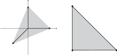
Figure 1. The fan and the convex polyhedron of ${\mathbb{C}}{\mathbb{P}}^{2}$.

By the previous lemma, each fixed point in the moduli space $\mathcal{M}_{0,m}^{A}({\mathbb{C}}{\mathbb{P}}^{2})$ has to “live on the boundary of the polyhedron $\Delta_{\varphi}$”, since the corners and the (one–dimensional) boundary components of the polyhedron correspond to fixed points respectively one–dimensional orbits of the torus action on ${\mathbb{C}}{\mathbb{P}}^{2}$. In fact, if one only looks at where the irreducible components and the marked points are mapped to in ${\mathbb{C}}{\mathbb{P}}^{2}$, one could abstractly think of such a fixed map as a graph that is wrapped around the polyhedron $\Delta_{\varphi}$.

In the following we will continue to use the notation of fans and its dual polyhedron $\Delta_{\varphi}$, e.g. we will label the vertices of the polyhedron $\Delta_{\varphi}$ by maximal cones $\sigma\in\Sigma^{(d)}$, etc. Remember that $\Delta_{\varphi}$ is also the moment polytope of $({X_{\Sigma}},\omega_{\varphi})$.

We will define three different kinds of graphs: a topological ${\mathcal{M}}_{0,m}^{A}({X_{\Sigma}})$–graph type ${{\Gamma}^{\text{top}}}$ describing the “image” of a fixed stable map on the polyhedron $\Delta_{\varphi}$, a ${\mathcal{M}}_{0,m}^{A}({X_{\Sigma}})$–graph type ${{\Gamma}^{\text{type}}}$ describing moreover the image of every irreducible component of a fixed stable map, and a ${\mathcal{M}}_{0,m}^{A}({X_{\Sigma}})$–graph ${\Gamma}$ containing all the data of a ${\mathcal{M}}_{0,m}^{A}({X_{\Sigma}})$–graph type plus the location of the marked points.

.

Let $\Sigma$ be a complete regular fan in $N\cong{\mathbb{Z}}^{d}$, and let $\Delta_{\varphi}$ be its dual polyhedron.

A topological ${\mathcal{M}}_{0,m}^{A}({X_{\Sigma}})$–graph type ${{\Gamma}^{\text{top}}}$ is a finite one–dimensional CW–complex with the following decorations:

1. A map $\sigma:\operatorname{Vert}({{\Gamma}^{\text{top}}})\longrightarrow\Sigma^{(d)}$ mapping each vertex $\mathfrak{v}$ of the graph to a vertex $\sigma(\mathfrak{v})$ of $\Delta_{\varphi}$;

2. A map $d:\operatorname{Edge}({{\Gamma}^{\text{top}}})\longrightarrow{\mathbb{Z}}_{>0}$, representing multiplicities of maps.

These decorations are subject to the following compatibility conditions:

1. The map $\sigma:\operatorname{Vert}({{\Gamma}^{\text{top}}})\longrightarrow\Sigma^{(d)}$ is injective;

2. If an edge $e\in\operatorname{Edge}({{\Gamma}^{\text{top}}})$ connects two vertices $\mathfrak{v}_{1},\mathfrak{v}_{2}\in\operatorname{Vert}({{\Gamma}^{\text{top}}})$ labeled $\sigma(\mathfrak{v}_{1})$ and $\sigma(\mathfrak{v}_{2})$, then the two cones must be different and have a common $(d-1)$–dimensional face: $\sigma(\mathfrak{v}_{1})\cap\sigma(\mathfrak{v}_{2})\in\Sigma^{(d-1)}$;

3. There is at most one edge connecting any two vertices: for any two edges $e_{1},e_{2}\in\operatorname{Edge}({{\Gamma}^{\text{top}}})$ with vertices $\mathfrak{v}_{i,1}$ and $\mathfrak{v}_{i,2}$, we have $\{\mathfrak{v}_{1,1},\mathfrak{v}_{1,2}\}\neq\{\mathfrak{v}_{2,1},\mathfrak{v}_{2,2}\}$;

4. The graph represents a stable map with homology class $A$:

   $$\sum_{\begin{array}[]{c}\scriptstyle e\in\operatorname{Edge}({{\Gamma}^{\text{top}}})\\ \scriptstyle\partial e=\{\mathfrak{v}_{1}(e),\mathfrak{v}_{2}(e)\}\end{array}}d(e)[V_{\sigma(\mathfrak{v}_{1})\cap\sigma(\mathfrak{v}_{2})}]=A,$$

   where $[V_{\sigma(\mathfrak{v}_{1})\cap\sigma(\mathfrak{v}_{2})}]$ is the homology class associated to this subvariety, and $\partial e=\{\mathfrak{v}_{1}(e),\mathfrak{v}_{2}(e)\}$ associates to an edge $e$ the two vertices $\mathfrak{v}_{1}(e),\mathfrak{v}_{2}(e)$ it connects.

A ${\mathcal{M}}_{0,m}^{A}({X_{\Sigma}})$–graph type ${{\Gamma}^{\text{type}}}$ is a finite one–dimensional CW-complex as above that is subject only to compatibility conditions (b) and (d), and additionally:

• The CW–complex ${{\Gamma}^{\text{type}}}$ contains no loops.

A ${\mathcal{M}}_{0,m}^{A}({X_{\Sigma}})$–graph ${\Gamma}$ is a ${\mathcal{M}}_{0,m}^{A}({X_{\Sigma}})$–graph type with an extra decoration:

• A map $S:\operatorname{Vert}({\Gamma})\mathrel{\smash{\mathop{\hbox to28.45274pt{\rightarrowfill}}}}\mathfrak{P}(\{1,\ldots,m\})$ associating to each vertex a set of marked points;

subject to the following additional compatibility conditions:

• For any two vertices $\mathfrak{v}_{1},\mathfrak{v}_{2}\in\operatorname{Vert}({\Gamma})$, the sets of associated marked points are disjoint: $S(\mathfrak{v}_{1})\cap S(\mathfrak{v}_{2})=\varnothing$;

• Every marked point is associated with some vertex:

  $$\bigcup_{\mathfrak{v}\in\operatorname{Vert}(\Sigma)}S(\mathfrak{v})=\{1,\ldots,m\}.$$

The are natural maps between the different categories of graphs that we will denote by $\operatorname{type}$ and $\operatorname{top}$:

.

Note, that in all cases above, there exists an induced map

$$\operatorname{Edge}(\cdot)\mathrel{\smash{\mathop{\hbox to28.45274pt{\rightarrowfill}}}}\Sigma^{(d-1)}$$

from edges of the graph to $(d-1)$–dimensional cones, or dually to edges of the polyhedron $\Delta_{\varphi}$.

In the remaining part of this section, we will consider ${\mathcal{M}}_{0,m}^{A}({X_{\Sigma}})$–graphs ${\Gamma}$ only, which we will simply call graphs when the underlying moduli stack is understood. In fact, each of these graphs describes a fixed point component in ${\mathcal{M}}_{0,m}^{A}({X_{\Sigma}})$, while graph types and topological graph types describe families of such fixed point components.

.

For a ${\mathcal{M}}_{0,m}^{A}({X_{\Sigma}})$–graph ${\Gamma}$, let $\deg$ be the function assigning to each vertex the number of its special points:

$$\deg:\operatorname{Vert}({\Gamma}) \mathrel{\smash{\mathop{\hbox to28.45274pt{\rightarrowfill}}}}{\mathbb{Z}}_{>0}$$

$$\mathfrak{v} \mapstochar\mathrel{\smash{\mathop{\hbox to28.45274pt{\rightarrowfill}}}}\#S(\mathfrak{v})+\#\{e\in\operatorname{Edge}({\Gamma})|\mathfrak{v}\in\partial e\}.$$

Furthermore, let $\mathcal{M}_{\Gamma}$ be the following product of Deligne–Mumford spaces:

$$\mathcal{M}_{\Gamma}:=\prod_{\mathfrak{v}\in\operatorname{Vert}({\Gamma})}\overline{{\mathcal{M}}}_{0,\deg(\mathfrak{v})},$$

where we formally set $\overline{{\mathcal{M}}}_{0,0}=\overline{{\mathcal{M}}}_{0,1}=\overline{{\mathcal{M}}}_{0,2}=\{pt.\}$, the universal curve above these space being by definition a point as well.

Then there exists a canonical family of $T_{N}$–fixed stable maps to ${X_{\Sigma}}$

$$\pi:\mathcal{C}_{\Gamma}\mathrel{\smash{\mathop{\hbox to28.45274pt{\rightarrowfill}}}}\mathcal{M}_{\Gamma},$$

fitting into the following diagram:

The image of $\mathcal{M}_{\Gamma}$ in ${\mathcal{M}}_{0,m}^{A}({X_{\Sigma}})$ is a fixed point component of the $T_{N}$–action on ${\mathcal{M}}_{0,m}^{A}({X_{\Sigma}})$.

Proof.

First we will describe the family of curves $\mathcal{C}_{\Gamma}\longrightarrow\mathcal{M}_{\Gamma}$. For each edge $e\in\operatorname{Edge}({\Gamma})$, let us number its vertices: $\partial e=\{\mathfrak{v}_{1}(e),\mathfrak{v}_{2}(e)\}$. For each such edge $e$ we also fix a map of degree one $\widetilde{f}_{e}:{\mathbb{P}}^{1}\longrightarrow V_{\sigma(\mathfrak{v}_{1})\cap\sigma(\mathfrak{v}_{2})}\subset{X_{\Sigma}}$, such that $\widetilde{f}_{e}(0)=V_{\sigma(\mathfrak{v}_{1})}$ and $\widetilde{f}_{e}(\infty)=V_{\sigma(\mathfrak{v}_{2})}$. We set $f_{e}:=\widetilde{f}_{e}\circ z^{d(e)}$ to obtain a map $f_{e}:{\mathbb{P}}^{1}\longrightarrow V_{\sigma(\mathfrak{v}_{1})\cap\sigma(\mathfrak{v}_{2})}$ of degree $d(e)$. Note that up to parametrization such a map is a unique. Also set $C_{e}:={\mathbb{P}}^{1}$. Let $\operatorname{val}:\operatorname{Vert}({\Gamma})\longrightarrow{\mathbb{Z}}_{>0}$ be the function assigning to each vertex the number of outgoing edges:

$$\operatorname{val}(\mathfrak{v}):=\#\{e\in\operatorname{Edge}({\Gamma})|\mathfrak{v}\in\partial e\}.$$

For each vertex $\mathfrak{v}\in\operatorname{Vert}(\mathfrak{v})$, chose an ordering of the set $\{e\in\operatorname{Edge}({\Gamma})|\mathfrak{v}\in\partial e\}$ of the outgoing edges:

$$e_{1}(\mathfrak{v}),\ldots,e_{\operatorname{val}(\mathfrak{v})}(\mathfrak{v}).$$

For convenience, let us number the vertices in the graph ${\Gamma}$: $\mathfrak{v}_{1},\ldots,\mathfrak{v}_{l}$, where $l=\#\operatorname{Vert}({\Gamma})$ is the number of vertices of the graph ${\Gamma}$. We will now glue together the stable map $(C;\underline{x};f)$ corresponding to a point $((C_{1},\underline{x_{1}}),\ldots,(C_{l},\underline{x_{l}}))$ in the product $\mathcal{M}_{\Gamma}=\prod_{i=1}^{l}\overline{{\mathcal{M}}}_{0,\deg(\mathfrak{v}_{i})}$. The curve $C$ is the union

$$C=\bigcup_{i=1}^{l}C_{i}\cup\bigcup_{e\in\operatorname{Edge}({\Gamma})}C_{e},$$

where the different parts are glued together along ordinary nodes according to the following rule:

• If $e\in\operatorname{Edge}({\Gamma})$, $\mathfrak{v}_{i}\in\partial e$ then $e=e_{j}(\mathfrak{v}_{i})$ for some $j$, and we will glue the $j$–th marked point $x_{i,j}$ of $C_{i}$ to $0$ of $C_{e}$, if $\mathfrak{v}_{i}=\mathfrak{v}_{1}(e)$, or to $\infty$ of $C_{e}$ otherwise.

The ordered set of marked points $\underline{x}$ is constituted of the “unused” marked points of the curves $(C_{i},\underline{x_{i}})$, i.e. the marked points at which we have not glued curves. The function $f:C\longrightarrow{X_{\Sigma}}$ is defined as follows:

$$f|_{C_{e}} :=f_{e}\quad\text{for each edge $e$,}$$

$$f|_{C_{i}} :=V_{\sigma(\mathfrak{v}_{i})}\quad\text{a constant function for each $\mathfrak{v}_{i}$.}$$

Let us explain this construction in plain English. Remember first, that the moduli spaces of stable maps to a point are isomorphic to Deligne–Mumford spaces:

$$\mathcal{M}^{0}_{0,m}(pt.)\cong\overline{{\mathcal{M}}}_{0,m}.$$

The points in $\mathcal{M}_{\Gamma}$ therefore encode the part of the fixed stable map that is send to fixed points in ${X_{\Sigma}}$. The parts of the fixed map that are send to 1–dimensional invariant subspaces are in fact rigid modulo parametrization, and their “topology” is encoded in the graph ${\Gamma}$.

Let us make a remark to the above construction for vertices $\mathfrak{v}_{i}$ with $\deg(\mathfrak{v}_{i})<3$: these curves $C_{i}$ are points that are glued to other points, i.e. they do not contribute irreducible components to the constructed curve $C$. Also, if $\deg(\mathfrak{v}_{i})=2$ and $\operatorname{val}(\mathfrak{v}_{i})=1$ (otherwise we must have $\operatorname{val}(\mathfrak{v}_{i})=0$ for $\deg(\mathfrak{v}_{i})<3$!), the remaining marked point of $C_{i}$ is identified with $0$ or $\infty$ of $C_{e}$, respectively.

The proof of the lemma is now straightforward. The family $\pi:\mathcal{C}_{\Gamma}\longrightarrow\mathcal{M}_{\Gamma}$ is the space constructed above — essentially it is the product of the universal curves over the Deligne–Mumford spaces modulo the constant curves corresponding to the edges of the graph.

Since the image of a fixed stable map is rigid, the constructed family maps onto a fixed point component of ${\mathcal{M}}_{0,m}^{A}({X_{\Sigma}})$. Also, all fixed point components can be obtained this way. ∎

The following notation will be useful in the sequel. A flag of a graph ${\Gamma}$ is a the pair of a vertex and an outgoing edge i.e. the set of flags is

$${\mathcal{F}}({\Gamma}):=\left\{(\mathfrak{v},e)\in\operatorname{Vert}({\Gamma})\times\operatorname{Edge}({\Gamma})|\mathfrak{v}\in\partial e\right\}.$$

For a graph type ${{\Gamma}^{\text{type}}}$ or a topological graph type ${{\Gamma}^{\text{top}}}$, flags are defined the same way.The labeling of the vertices $\sigma:\operatorname{Vert}({\Gamma})\longrightarrow\Sigma^{(d)}$ by $d$–cones induces a corresponding labeling of flags by

$$\sigma((\mathfrak{v},\star)):=\sigma(\mathfrak{v})\qquad\text{for $(\mathfrak{v},\star)\in{\mathcal{F}}$}.$$

We will also use the projections of flags to vertices and edges which we will denote by

$$\mathfrak{v}(F) =\mathfrak{v}\quad\text{for $(\mathfrak{v},\star)=F\in{\mathcal{F}}$ and $\mathfrak{v}\in\operatorname{Vert}$}$$

$$e(F) =e\quad\text{for $(\star,e)=F\in{\mathcal{F}}$ and $e\in\operatorname{Edge}$.}$$

Finally we define the following subsets of $\operatorname{Vert}$ and $\operatorname{Edge}$:

$$\operatorname{Vert}_{t,s} :=\left\{\mathfrak{v}\in\operatorname{Vert}|\operatorname{val}(\mathfrak{v})=t,\deg(\mathfrak{v})=t+s\right\}$$

$$\operatorname{Vert}_{t} :=\left\{\mathfrak{v}\in\operatorname{Vert}|\deg(\mathfrak{v})=t\right\}$$

$${\mathcal{F}}_{t,s} :=\left\{(\mathfrak{v},\star)\in{\mathcal{F}}|\mathfrak{v}\in\operatorname{Vert}_{s,t}\right\}$$

$${\mathcal{F}}_{t} :=\left\{(\mathfrak{v},\star)\in{\mathcal{F}}|\mathfrak{v}\in\operatorname{Vert}_{t}\right\}.$$

.

We do not include marked points as flags, in contrary to Kontsevich [Kon95] and Graber and Pandharipande [GP99]. However, in the definition of the subsets $\operatorname{Vert}_{t,s}$ etc. the number of marked points at a vertex $\mathfrak{v}$ does enter via the function $\deg$.

.

Let us describe one example in great detail to familiarize with the notions defined so far. We will look at the two dimensional toric variety that is given by the following fan in ${\mathbb{Z}}^{2}$, $e_{1}$ and $e_{2}$ being a ${\mathbb{Z}}$–base:

$$v_{1}=e_{1},\quad v_{2}=e_{2},\quad v_{3}=-e_{1}+e_{2},\quad v_{4}=-e_{2}$$

$${\mathcal{P}}=\left\{\{v_{1},v_{3}\},\{v_{2},v_{4}\}\right\}.$$

The fan $\Sigma$ having the $1$–skeleton $\Sigma^{(1)}=\{v_{1},\ldots,v_{4}\}$ and the set of primitive collections $\mathcal{P}$ is shown in figure 2, as well as its polyhedron corresponding to the strictly convex upper support function $\varphi=c_{1}({X_{\Sigma}})$. The toric variety ${X_{\Sigma}}$ constructed from $\Sigma$ is the Hirzebruch surface $F_{1}={\mathbb{P}}({\mathcal{O}}_{{\mathbb{P}}^{1}}(1)\oplus 1)\cong\widetilde{{\mathbb{P}}^{2}}$, which is isomorphic to ${\mathbb{P}}^{2}$ blown up at one point.

Figure 2. The fan of ${\mathbb{P}}({\mathcal{O}}_{{\mathbb{P}}^{1}}(1)\oplus 1)$, and its polyhedron for $\varphi=c_{1}$.

Before we give a graph corresponding to a fixed point in ${\mathcal{M}}_{0,m}^{A}({X_{\Sigma}})$ of this toric variety, let us analyze the homology and cohomology in degree two of ${X_{\Sigma}}$. We have seen above, that (integral) degree–$2$ cohomology classes are given by $\Sigma$–piecewise linear functions, factored out by linear functions $\psi\in M=\operatorname{Hom}(N,{\mathbb{Z}})$. A function $\varphi\in PL(\Sigma)$ is given by its values on the $1$–skeleton, an element $\psi\in M$ by its values on $e_{1},e_{2}$. Hence for a $\varphi$ representing an equivalence class $[\varphi]\in PL(\Sigma)/M$ we can assume

$$\varphi(v_{1})=\varphi(v_{2})=0,\qquad\varphi(v_{3}),\varphi(v_{4})\in{\mathbb{Z}}.$$

Such a class $[\varphi]$ is in the Kähler cone if it satisfies

$$\varphi(v_{1})+\varphi(v_{3})>\varphi(v_{1}+v_{3})\quad\text{and}\quad\varphi(v_{2})+\varphi(v_{4})>\varphi(v_{2}+v_{4})$$

that is, with the choices above,

$$\varphi(v_{3})>0\quad\text{and}\quad\varphi(v_{4})>0.$$

Note, that this implies in particular, that the first Chern class $c_{1}({X_{\Sigma}})$ of ${X_{\Sigma}}$ is indeed a Kähler class.

For the degree–$2$ homology of ${X_{\Sigma}}$, notice that the ${\mathbb{Z}}$–module

$$R(\Sigma)=\left\{(\lambda_{1},\ldots,\lambda_{n})\,|\,\lambda_{1}v_{1}+\ldots+\lambda_{n}v_{n}=0\right\}$$

is generated by the elements corresponding to the equations

$$\quad v_{2}+v_{4}=0\quad\text{and}\quad v_{1}+v_{3}+v_{4}=0$$

that is by the elements

$$\lambda^{1}:=(0,1,0,1)\quad\text{and}\quad\lambda^{2}:=(1,0,1,1).$$

To find out the homology classes of the four one dimensional $T_{N}$–invariant subvarieties $V_{\langle v_{1}\rangle},\ldots,V_{\langle v_{4}\rangle}$, the Poincaré dual cohomology classes $[\varphi_{1}],\ldots,[\varphi_{4}]$ of which are given by

$$\tilde{\varphi}_{i}(v_{j})=\delta_{ij}=\left\{\begin{array}[]{ll}1&\text{if i=j}\\[3.0pt] 0&\text{otherwise.}\end{array}\right.$$

Hence, again by Poincaré duality, we get

$$[V_{\langle v_{1}\rangle}]=\lambda^{2},\quad[V_{\langle v_{2}\rangle}]=\lambda^{1},\quad[V_{\langle v_{3}\rangle}]=\lambda^{2},\quad[V_{\langle v_{4}\rangle}]=\lambda^{1}+\lambda^{2}.$$

Therefore, any ${\mathcal{M}}_{0,m}^{A}({X_{\Sigma}})$–graph ${\Gamma}$ has to “live” on the decorated $1$–skeleton $\Upsilon_{\Sigma}$ of the moment polytope $\Delta_{\varphi}$ shown in figure 4 in the sense that there is a map $f:{\Gamma}\longrightarrow\Upsilon_{\Sigma}$ of one–dimensional CW–complexes such that the decorations $\sigma:\operatorname{Vert}({\Gamma})\longrightarrow\Sigma^{(d)}$ of the vertices of ${\Gamma}$ with fixed points in ${X_{\Sigma}}$ are induced from the decorations of the vertices of $\Upsilon_{\Sigma}$. Figure 4 shows two ${\mathcal{M}}_{0,0}^{A}({X_{\Sigma}})$–graphs for the homology class $A=2\lambda^{2}+\lambda^{1}$. Note that there are other possible graphs for this class.

Figure 3. The $1$–skeleton $\Upsilon_{\Sigma}$ of the moment polytope $\Delta_{v}arphi$.

Figure 4. Two different graph types for $A=2\lambda^{2}+\lambda^{1}$.

6.3. Automorphisms of fixed point components

For a family $\pi:\mathcal{C}_{\Gamma}\longrightarrow\mathcal{M}_{\Gamma}$ of $T_{N}$–fixed stable maps to ${X_{\Sigma}}$ as constructed above, there are two different sources of $\pi$–equivariant automorphisms we have to consider: automorphisms of the family $\pi:\mathcal{C}_{\Gamma}\longrightarrow\mathcal{M}_{\Gamma}$ itself, and automorphisms of this family as substack of ${\mathcal{M}}_{0,m}^{A}({X_{\Sigma}})$.

The first are given by automorphisms of the ${\mathcal{M}}_{0,m}^{A}({X_{\Sigma}})$–graph ${\Gamma}$ (with its decorations), since by considering products of Deligne–Mumford spaces we have ordered the nodes. All other possible sources of automorphisms have already been moded out by taking choices in the proof of Proposition 6.2.

The extra automorphisms stemming from the map to the stack ${\mathcal{C}}_{0,m}^{A}({X_{\Sigma}})\longrightarrow{\mathcal{M}}_{0,m}^{A}({X_{\Sigma}})$ is a cyclic permutation of the branches of the degree–$d(e)$ maps $f_{e}$. This ${\mathbb{Z}}_{d(e)}$–action is trivial on $\mathcal{M}_{\Gamma}$, but not on its deformations, underlining the “orbifold character” of the moduli stack ${\mathcal{M}}_{0,m}^{A}({X_{\Sigma}})$.

.

The automorphism group ${\bf A}_{\Gamma}$ of $\pi:\mathcal{C}_{\Gamma}\longrightarrow\mathcal{M}_{\Gamma}$ fits into the following exact sequence of groups

$$1\longrightarrow\prod_{e\in\operatorname{Edge}}{\mathbb{Z}}_{d(e)}\longrightarrow{\bf A}_{\Gamma}\longrightarrow\operatorname{Aut}({\Gamma})\longrightarrow 1,$$

where $\operatorname{Aut}({\Gamma})$ acts naturally on $\prod_{e}{\mathbb{Z}}_{d(e)}$, ${\bf A}_{\Gamma}$ being the semi–direct product. The induced map

$$\gamma/{\bf A}_{\Gamma}:{\mathcal{M}}_{\Gamma}/{\bf A}_{\Gamma}\mathrel{\smash{\mathop{\hbox to28.45274pt{\rightarrowfill}}}}{\mathcal{M}}_{0,m}^{A}({X_{\Sigma}})$$

is a closed immersion of Deligne–Mumford stacks. Furthermore, the image is a component of the $T_{N}$–fixed point stack of ${\mathcal{M}}_{0,m}^{A}({X_{\Sigma}})$. $\square$

6.4. Weights on fixed point components

At the end of this section, we will compute the weight of the $T_{N}$–action on the irreducible $T_{N}$–invariant divisors $V_{\tau}$, $\tau\in\Sigma^{(d-1)}$, and subsequently we will derive the weight of the action on a non–constant map

$$f:{\mathbb{P}}^{1}\mathrel{\smash{\mathop{\hbox to28.45274pt{\rightarrowfill}}}}V_{\tau}\subset{X_{\Sigma}},\qquad\tau\in\Sigma^{(d-1)}$$

represented by an edge $e$ in a ${\mathcal{M}}_{0,m}^{A}({X_{\Sigma}})$–graph ${\Gamma}$. Let $\sigma_{1},\sigma_{2}\in\Sigma^{(d)}$ be two $d$–cones in $\Sigma$ that have a common $(d-1)$–face $\tau\in\Sigma^{(d-1)}$. Notice that $V_{\tau}$ is the closure of a one–dimensional orbit of the $T_{N}$ action, compactified with the two fixed points of this action given by the two $d$–cones $\sigma_{1}$ and $\sigma_{2}$. So, the $T_{N}$ action reduces to a ${\mathbb{C}}^{*}$–action on $V_{\tau}$, that is to the action of a subtorus ${\mathbb{C}}^{*}\cong T_{\tau}\cong T_{N}$ of $T_{N}$. The torus $T_{\tau}$ is the image of the map

$$\beta_{\tau}:({\mathbb{C}}^{*})^{n}\mathrel{\smash{\mathop{\hbox to28.45274pt{\rightarrowfill}}}}T_{N}\mathrel{\smash{\mathop{\hbox to28.45274pt{\rightarrowfill}}}}T_{\tau}$$

given by the quotient map $T_{N}=({\mathbb{C}}^{*})^{n}/\mathbf{D}(\Sigma)$ followed by restriction to $V_{\tau}$. Thus, we can write elements of $T_{\tau}$ as equivalence classes of elements in $({\mathbb{C}}^{*})^{n}$ by the map $\beta_{\tau}$.

.

Let $\sigma_{1},\sigma_{2},\tau\in\Sigma$ as above. Let $v_{i_{1}},\ldots,v_{i_{d-1}}$ be the generators of the common face $\tau=\sigma_{1}\cap\sigma_{2}$, such that

$$\sigma_{1} =\langle v_{i_{1}},\ldots,v_{i_{d-1}},v_{l_{1}(\tau)}\rangle$$

$$\sigma_{2} =\langle v_{i_{1}},\ldots,v_{i_{d-1}},v_{l_{2}(\tau)}\rangle.$$

Let ${\omega}_{1},\ldots,{\omega}_{n}$ be the weights of a diagonal action of $({\mathbb{C}}^{*})^{n}$ on ${\mathbb{C}}^{n}$ with respect to the standard basis. The induced ${\mathbb{C}}^{*}$–action on the subvariety $V_{\tau}$, has weight ${\omega}^{\sigma_{1}}_{\sigma_{2}}$ at the point $V_{\sigma_{1}}$:

$${\omega}^{\sigma_{1}}_{\sigma_{2}}:=\sum_{j=1}^{n}\langle v_{j},u_{d}\rangle{\omega}_{j},$$

where $u_{1},\ldots,u_{d}$ is the basis of $M=\operatorname{Hom}(N,{\mathbb{Z}})$ dual to $v_{i_{1}},\ldots,v_{i_{d-1}},v_{l_{1}(\tau)}$.

Proof.

The $d$–dimensional cone $\sigma_{1}$ gives a local chart $U_{\sigma_{1}}$ of our toric variety ${X_{\Sigma}}$, and the coordinates on $U_{\sigma_{1}}$ are given by (cf. proposition 5.1):

$$x_{1}^{\sigma_{1}}=\prod_{j}z_{j}^{\langle v_{j},u_{1}\rangle},\quad\ldots\quad,x_{d}^{\sigma_{1}}=\prod_{j}z_{j}^{\langle v_{j},u_{d}\rangle},$$

The $1$–dimensional submanifold corresponding to $\tau$ is given by the equations $z_{i_{1}}=\ldots=z_{i_{d-1}}=0$. In the coordinates of $U_{\sigma_{1}}$, these equations are equivalent to

$$x_{1}^{\sigma_{1}}=\ldots=x_{d-1}^{\sigma_{1}}=0.$$

Hence we have to look at the $({\mathbb{C}}^{*})^{d}$–action on the $d^{th}$ co–ordinate. Thus the action of $(t_{1},\ldots,t_{n})\in({\mathbb{C}}^{*})^{n}$ on $V_{\tau}$ is given by

$$(t_{1},\ldots,t_{n})\cdot x_{d}^{\sigma_{1}} =\prod_{j}(t_{j}z_{j})^{\langle v_{j},u_{d}\rangle}$$

$$=\left(\prod_{j}t_{j}^{\langle v_{j},u_{d}\rangle}\right)\cdot\left(\prod_{j}z_{j}^{\langle v_{j},u_{d}\rangle}\right)$$

$$=t^{{\omega}^{\sigma_{1}}_{\sigma_{2}}}x_{d},$$

using multi–index notation in the last line. Hence the weight of the action on $V_{\tau}$ is indeed $\sum_{j}\langle v_{j},u_{d}\rangle{\omega}_{j}$ in the chart $U_{\sigma_{1}}$. ∎

The lemma above gives in particular the $T_{N}$–action on a the component of a fixed stable curve that is mapped to $V_{\tau}$:

.

Let $e\in\operatorname{Edge}({\Gamma})$ be an edge of the ${\mathcal{M}}_{0,m}^{A}({X_{\Sigma}})$–graph ${\Gamma}$, and $\mathfrak{v}_{1},\mathfrak{v}_{2}\in\partial e$ be the vertices at its two ends. Let $\sigma_{i}=\sigma(\mathfrak{v}_{i})$ be the $d$–cones of the vertices $\mathfrak{v}_{i}$, and $\tau(e)=\sigma_{1}\cap\sigma_{2}$ its common $(d-1)$–face, that are generated by

$$\sigma_{1}=\sigma(\mathfrak{v}_{1}) =\langle v_{i_{1}},\ldots,v_{i_{d-1}},v_{l_{1}(e)}\rangle$$

$$\sigma_{2}=\sigma(\mathfrak{v}_{2}) =\langle v_{i_{1}},\ldots,v_{i_{d-1}},v_{l_{2}(e)}\rangle.$$

For a $T_{N}$–fixed stable map $(C;x_{1},\ldots,x_{m};f)\in{\mathcal{M}}_{\Gamma}\subset{\mathcal{M}}_{0,m}^{A}({X_{\Sigma}})$, let $C_{e}$ be the irreducible component of $C$ corresponding to the edge $e$. Let $F:=(\mathfrak{v}_{1},e)\in{\mathcal{F}}$ be the flag of the edge $e$ at the vertex $\mathfrak{v}_{1}$. At the point $p_{F}:=f^{-1}(V_{\sigma(\mathfrak{v}_{1})})\cap C_{e}$, the pull back to $C_{e}$ by $f$ of the $T_{N}$–action on $V_{\tau(e)}$ has the weight ${\omega}_{F}$ at $p_{F}$:

$${\omega}_{F}:=\frac{1}{d_{e}}\sum_{j=1}^{n}\langle v_{j},u_{d}\rangle{\omega}_{j},$$

where $d_{e}$ is the multiplicity of the component $C_{e}$, and $u_{1},\ldots,u_{d}$ is the basis of $M=\operatorname{Hom}(N,{\mathbb{Z}})$ dual to $v_{i_{1}},\ldots,v_{i_{d-1}},v_{l_{1}(e)}$.

Proof.

The action of $T_{N}$ on $C_{e}$ is just the pull back by $f$ of the action on $V_{\tau}$. Since $f$ has multiplicity $d_{e}$, the formula follows immediately from lemma 6.4. ∎

We will introduce some further notation, grouping together certain weights on the one–dimensional $T_{N}$–invariant subvariety of ${X_{\Sigma}}$, or more general on a ${\mathcal{M}}_{0,m}^{A}({X_{\Sigma}})$–graph ${\Gamma}$. First of all, we will write $\sigma_{1}\diamond\sigma_{2}$ for the property of $\sigma_{1}$ and $\sigma_{2}$ having a common $(d-1)$–dimensional proper face:

$$\sigma_{1}\diamond\sigma_{2}\Longleftrightarrow\sigma_{1},\sigma_{2}\in\Sigma^{(d)}\medspace\text{and}\medspace\sigma_{1}\cap\sigma_{2}\in\Sigma^{(d-1)}.$$

The total weight of a $d$–dimensional cone $\sigma$ is defined to be

$${\omega}_{\text{total}}^{\sigma}:=\prod_{\gamma\diamond\sigma}{\omega}_{\gamma}^{\sigma}.$$

Note that ${\omega}_{\text{total}}^{\sigma}$ is in fact a polynomial in the generators of $\mathfrak{t}^{n}$: ${\omega}_{\text{total}}^{\sigma}\in{\mathbb{Z}}[{\omega}_{1},\ldots,{\omega}_{n}]$.

7. The virtual normal bundle for toric varieties

In this section we analyze Graber and Pandharipande’s virtual normal bundle to the fixed point components of the moduli space of stable maps for the natural $({\mathbb{C}}^{*})^{n}$–action on a toric variety, hence generalizing Graber and Pandharipande’s example for projective space ${\mathbb{C}}{\mathbb{P}}^{n}$ ([GP99]), and we will derive our main result. Contrary to their calculations for ${\mathbb{C}}{\mathbb{P}}^{n}$, however, we will restrict ourselves here to genus zero stable maps.

So let ${X_{\Sigma}}$ be a smooth projective complex variety. Remember from section 3.2, that for the cohomology sheaves of the dual natural perfect obstruction theory $E_{\bullet}$ for our moduli stack ${\mathcal{M}}_{0,m}^{A}({X_{\Sigma}})$ of stable maps

$$0\mathrel{\smash{\mathop{\hbox to28.45274pt{\rightarrowfill}}}}\mathcal{T}^{0}\mathrel{\smash{\mathop{\hbox to28.45274pt{\rightarrowfill}}}}E_{0}\mathrel{\smash{\mathop{\hbox to28.45274pt{\rightarrowfill}}\limits^{\textstyle d}}}E_{1}\mathrel{\smash{\mathop{\hbox to28.45274pt{\rightarrowfill}}}}\mathcal{T}^{1}\mathrel{\smash{\mathop{\hbox to28.45274pt{\rightarrowfill}}}}0,$$ (7)

the sheaves $\mathcal{T}^{i}$ are given by:

$$\mathcal{T}^{i}=\underline{\operatorname{Ext}}^{i}_{\pi}([f^{*}\Omega^{1}_{X}\longrightarrow\Omega^{1}_{{\mathcal{C}}_{0,m}^{A}({X_{\Sigma}})/{\mathcal{M}}_{0,m}^{A}({X_{\Sigma}})}(D)],{\mathcal{O}}_{{\mathcal{C}}_{0,m}^{A}({X_{\Sigma}})}),\quad i=0,1.$$

As before we will sometimes write $\mathcal{M}$ and $\mathcal{C}$ for the moduli space ${\mathcal{M}}_{0,m}^{A}({X_{\Sigma}})$ and its universal curve ${\mathcal{C}}_{0,m}^{A}({X_{\Sigma}})$, respectively, if no confusion can arise.

.

The sheaves $\mathcal{T}^{i}$ fit into the following exact sequence:

$$\begin{split}0&\mathrel{\smash{\mathop{\hbox to28.45274pt{\rightarrowfill}}}}\underline{\operatorname{Hom}}_{\pi}(\Omega^{1}_{\mathcal{C}/\mathcal{M}}(D),{\mathcal{O}}_{\mathcal{C}})\mathrel{\smash{\mathop{\hbox to28.45274pt{\rightarrowfill}}}}\underline{\operatorname{Hom}}_{\pi}(f^{*}\Omega^{1}_{X},{\mathcal{O}}_{\mathcal{C}})\mathrel{\smash{\mathop{\hbox to28.45274pt{\rightarrowfill}}}}\mathcal{T}^{0}\mathrel{\smash{\mathop{\hbox to28.45274pt{\rightarrowfill}}}}\\ &\mathrel{\smash{\mathop{\hbox to28.45274pt{\rightarrowfill}}}}\underline{\operatorname{Ext}}^{1}_{\pi}(\Omega^{1}_{\mathcal{C}/\mathcal{M}}(D),{\mathcal{O}}_{\mathcal{C}})\mathrel{\smash{\mathop{\hbox to28.45274pt{\rightarrowfill}}}}\underline{\operatorname{Ext}}_{\pi}^{1}(f^{*}\Omega^{1}_{X},{\mathcal{O}}_{\mathcal{C}})\mathrel{\smash{\mathop{\hbox to28.45274pt{\rightarrowfill}}}}\mathcal{T}^{1}\mathrel{\smash{\mathop{\hbox to28.45274pt{\rightarrowfill}}}}0.\\ \end{split}$$ (8)

Proof.

Let $\mathcal{K}^{\bullet}$ be the complex $\mathcal{K}^{\bullet}=[f^{*}\Omega^{1}_{X}\longrightarrow\Omega^{1}_{{\mathcal{C}}_{0,m}^{A}({X_{\Sigma}})/{\mathcal{M}}_{0,m}^{A}({X_{\Sigma}})}(D)]$ indexed at $-1$ and $0$. It fits into the following short exact sequence:

$$0\mathrel{\smash{\mathop{\hbox to28.45274pt{\rightarrowfill}}}}\Omega^{1}_{\mathcal{C}/\mathcal{M}}(D)\mathrel{\smash{\mathop{\hbox to28.45274pt{\rightarrowfill}}}}\mathcal{K}^{\bullet}\mathrel{\smash{\mathop{\hbox to28.45274pt{\rightarrowfill}}}}f^{*}\Omega^{1}_{X}[1]\mathrel{\smash{\mathop{\hbox to28.45274pt{\rightarrowfill}}}}0.$$

The corresponding long exact sequence of higher direct image sheaves corresponding to $\pi:{\mathcal{C}}_{0,m}^{A}({X_{\Sigma}})\longrightarrow{\mathcal{M}}_{0,m}^{A}({X_{\Sigma}})$ is then (8 where exactness on the left, i.e. the injectivity of the map ${\underline{\operatorname{Hom}}}_{\pi}(\Omega^{1}_{\mathcal{C}/\mathcal{M}}(D),{\mathcal{O}}_{\mathcal{C}})\longrightarrow{\underline{\operatorname{Hom}}}_{\pi}(f^{*}\Omega^{1}_{X},{\mathcal{O}}_{\mathcal{C}})$ induced by the natural map $f^{*}\Omega^{1}_{X}\longrightarrow\Omega^{1}_{\mathcal{C}/\mathcal{M}}\longrightarrow\Omega^{1}_{\mathcal{C}/\mathcal{M}}(D)$ is equivalent to the stability of the map $f:{\mathcal{C}}_{0,m}^{A}({X_{\Sigma}})\longrightarrow X$ (cf. lemma 2.4 and the remark following the lemma). Exactness on the right of the long exact sequence follows from the fact of the fibers of ${\mathcal{C}}_{0,m}^{A}({X_{\Sigma}})\longrightarrow{\mathcal{M}}_{0,m}^{A}({X_{\Sigma}})$ being curves. ∎

Now, let $\mathcal{M}_{\Gamma}$ be a fixed point component in the moduli stack of stable maps ${\mathcal{M}}_{0,m}^{A}({X_{\Sigma}})$, and $\pi_{\Gamma}:\mathcal{C}_{\Gamma}\longrightarrow\mathcal{M}_{\Gamma}$ its universal curve. By lemma 3.2, we know that the restriction of the long exact sequence (8) to the fixed point component $\mathcal{M}_{\Gamma}$ becomes:

$$\begin{split}0&\longrightarrow\underline{\operatorname{Hom}}_{\pi_{\Gamma}}(\Omega^{1}_{\mathcal{C}_{\Gamma}/\mathcal{M}_{\Gamma}}(D),{\mathcal{O}}_{\mathcal{C}_{\Gamma}})\longrightarrow\underline{\operatorname{Hom}}_{\pi_{\Gamma}}(f_{\Gamma}^{*}\Omega^{1}_{X},{\mathcal{O}}_{\mathcal{C}_{\Gamma}})\longrightarrow\mathcal{T}^{0}|_{\mathcal{M}_{\Gamma}}\longrightarrow\\ &\longrightarrow\underline{\operatorname{Ext}}^{1}_{\pi_{\Gamma}}(\Omega^{1}_{\mathcal{C}_{\Gamma}/\mathcal{M}_{\Gamma}}(D_{\Gamma}),{\mathcal{O}}_{\mathcal{C}_{\Gamma}})\longrightarrow\underline{\operatorname{Ext}}^{1}_{\pi_{\Gamma}}(f_{\Gamma}^{*}\Omega^{1}_{X},{\mathcal{O}}_{\mathcal{C}_{\Gamma}})\longrightarrow\mathcal{T}^{1}|_{\mathcal{M}_{\Gamma}}\longrightarrow 0.\\ \end{split}$$ (9)

In particular, if we restrict to a single stable map $(C;\underline{x};f)\in\mathcal{M}_{\Gamma}$, we get:

$$\begin{split}0&\longrightarrow\operatorname{Ext}^{0}(\Omega_{C}(\underline{x}),{\mathcal{O}}_{C})\longrightarrow H^{0}(C,f^{*}TX)\longrightarrow{\mathcal{T}}^{0}|_{\{C\}}\longrightarrow\\ &\longrightarrow\operatorname{Ext}^{1}(\Omega_{C}(\underline{x}),{\mathcal{O}}_{C})\longrightarrow H^{1}(C,f^{*}TX)\longrightarrow{\mathcal{T}}^{1}|_{\{C\}}\longrightarrow 0.\\ \end{split}$$ (10)

To determine the virtual normal bundle for the torus action on our toric variety, we will have to fulfill the moving parts of $\mathcal{T}^{i}_{\Gamma}=\mathcal{T}^{i}|_{\mathcal{M}_{\Gamma}}$, hence the moving parts in the sequence (9). We will call the $i^{th}$ term of this long exact sequence by $B_{i}$, and the moving part (with respect to the induced torus action) by $B_{i}^{\text{move}}$. Remember, that the virtual normal bundle $N_{\Gamma}^{\text{vir}}$ is the moving part of the induced complex $E_{\bullet,{\Gamma}}$, that is

$$e^{T_{N}}(N_{\Gamma}^{\text{vir}})=e^{T_{N}}(E_{0,{\Gamma}}^{\text{move}}-E_{1,{\Gamma}}^{\text{move}})=e^{T_{N}}({\mathcal{T}}_{\Gamma}^{0,{\text{move}}}-{\mathcal{T}}_{\Gamma}^{1,{\text{move}}}),$$

where the second equation holds because of the exact sequence (7). Now, applying the long exact sequence (9) we obtain for the equivariant Euler class of the virtual normal class $N^{vir}$ the following formula:

$$e^{T_{N}}(N_{\Gamma}^{\text{virt}})=\frac{e^{T_{N}}(B_{2}^{\text{move}})e^{T_{N}}(B_{4}^{\text{move}})}{e^{T_{N}}(B_{1}^{\text{move}})e^{T_{N}}(B_{5}^{\text{move}})}\in H^{*}_{T_{N}}(X,{\mathbb{Q}}).$$ (11)

The notation is indeed correct, since the $B_{i}^{\text{move}}$, $i=1,2,4,5$, are vector bundles on ${\mathcal{M}}_{\Gamma}$! This does not apply in general to the fixed parts of these sheaves, or even to the sheaves ${\mathcal{T}}^{i}_{\Gamma}$. So actually, at least for the moving parts, we look at a long exact sequence of the kind of (10).

In the following, we will calculate the contributions of the four bundles to the equivariant Euler class of the virtual normal bundle.

7.1. Computation of the equivariant Euler class of $B_{1}^{\text{move}}$

This bundle almost never contributes to the virtual normal bundle — indeed we will show the following lemma:

.

The $T_{N}$–equivariant Euler class of $B_{1}^{\text{move}}$ is given by

$$e^{T_{N}}(B_{1}^{\text{move}})=\prod_{F\in{\mathcal{F}}_{1}}{\omega}_{F}.$$ (12)

Proof.

The bundle $B_{1}=\operatorname{Ext}^{0}(\Omega_{C}(D),{\mathcal{O}}_{C})=\operatorname{Aut}_{\infty}(C)$ parameterizes infinitesimal automorphisms of the pointed domain. The induced $T_{N}$–action on $\operatorname{Aut}(C)$ is obviously trivial on all automorphism $\varphi$ of $C$ that restrict to the identity $\varphi_{|C_{e}}=\operatorname{id}_{C_{e}}$ on all irreducible components $C_{e}$ corresponding to edges $e\in\operatorname{Edge}({\Gamma})$ in the graph ${\Gamma}$. Thus, the moving part of $\operatorname{Aut}_{\infty}(C)$ splits into

$$\operatorname{Aut}_{\infty}^{\text{move}}(C)=\bigoplus_{e\in\operatorname{Edge}({\Gamma})}\operatorname{Aut}_{\infty}^{\text{move}}(C_{e}).$$

Note in particular, that the bundle $\operatorname{Aut}_{\infty}^{\text{move}}(C)$ is topologically trivial on ${\mathcal{M}}_{\Gamma}$ since it only depends on the irreducible components that are not mapped to a point, i.e. that are rigid in ${\mathcal{M}}_{\Gamma}$.

The $\operatorname{Aut}_{\infty}^{\text{move}}(C_{e})$ obviously depend on the special points of the irreducible component $C_{e}$, i.e. on the way it is “glued” at the nodes corresponding to the vertices $\mathfrak{v}_{1}(e)$ and $\mathfrak{v}_{2}(e)$ of the edge $e$. Since we only look at moduli stacks of stable maps with at least three marked points, we can exclude the two special cases (cf. figures 7 and 7) where both vertices are in $\operatorname{Vert}_{1,0}$, or where one is in $\operatorname{Vert}_{1,0}$ and the other in $\operatorname{Vert}_{1,1}$. We are left with two cases:

Case 1:

One edge in $\operatorname{Vert}_{1,0}$, the other in $\operatorname{Vert}_{2,0}\cup\operatorname{Vert}_{\geq 3}$ — Without loss of generality we can assume that $\mathfrak{v}_{1}(e)\in\operatorname{Vert}_{1,0}$. In this case, $C_{e}$ corresponds to a non–contracted ${\mathbb{P}}^{1}$ attached to another non–contracted (or, in the $\operatorname{Vert}_{\geq 3}$–case, contracted) component (see figure 7). Therefore we have to look at Möbius transformations that fix one point, infinity say:

$$[x_{1}:x_{2}]\mapsto[ax_{1}+bx_{2}:x_{2}].$$

Let $F\in{\mathcal{F}}_{1}$ be the flag corresponding to $\mathfrak{v}_{1}$. We have seen above that the induced $T_{N}$–action on $C_{e}$ is given by (using again multi–index notation):

$$t\cdot[x_{1}:x_{2}]=[t^{{\omega}_{F}}x_{1}:x_{2}],$$

since the co–ordinate $x_{1}$ corresponds to the chart of the flag $F$ (while $x_{2}$ corresponds to the chart around infinity, i.e. at the vertex $\mathfrak{v}_{2}$. To determine the $T_{N}$–action on the group $\operatorname{Aut}_{\infty}(C_{e})$ of infinitesimal automorphisms of $C_{e}$, we have to compute:

$$t\cdot(a,b)\cdot t^{-1}\cdot[x_{1}:x_{2}] =t\cdot(a,b)\cdot[t^{-{\omega}_{F}}x_{1}:x_{2}]$$

$$=t\cdot[at^{-{\omega}_{F}}x_{1}+bx_{2}:x_{2}]$$

$$=[ax_{1}+t^{{\omega}_{F}}bx_{2}:x_{2}]$$

$$=(a,t^{{\omega}_{F}}b)\cdot[x_{1}:x_{2}],$$

hence the $T_{N}$–action on an automorphism of $C_{e}$ is given by:

$$t\cdot(a,b)=(a,t^{{\omega}_{F}}b).$$

The moving part of $\operatorname{Aut}_{\infty}(C_{e})$ is thus spanned by the second co–ordinate, and the weight of the action there is ${\omega}_{F}$ — in this case we have:

$$e^{T_{N}}(\operatorname{Aut}_{\infty}(C_{e})^{\text{move}})={\omega}_{F}.$$

Case 2:

Neither vertex is in $\operatorname{Vert}_{1,0}$ — In this case, any automorphism of $C$ restricts to an automorphism on $C_{e}$ that fixes the two points corresponding to the special points of the vertices $\mathfrak{v}_{1}$ and $\mathfrak{v}_{2}$. Any such automorphism on $C_{e}$ (w. l. o. g. we take the two points to be zero and infinity) has to look like

$$[x_{1}:x_{2}]\mapstochar\mathrel{\smash{\mathop{\hbox to28.45274pt{\rightarrowfill}}}}[ax_{1}:x_{2}],$$

where $a\neq 0$ is a non-negative integer. With the same analysis as above of the $T_{N}$–action on such automorphism $a$, we see that the $T_{N}$–action on $\operatorname{Aut}_{\infty}(C_{e})$ is trivial, i.e.

$$\operatorname{Aut}_{\infty}^{\text{move}}(C_{e})=(0).$$

∎

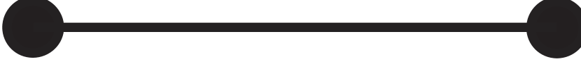
Figure 5. A graph with two vertices in $\operatorname{Vert}_{1,0}$.

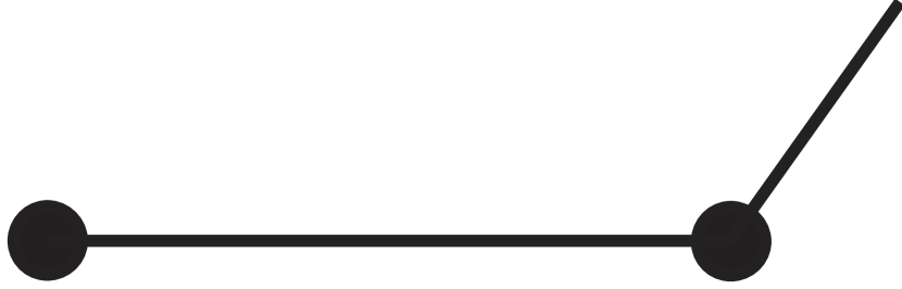
Figure 6. A graph with the left vertex in $\operatorname{Vert}_{1,0}$ and the right vertex in $\operatorname{Vert}_{1,1}$.

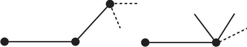
Figure 7. Two examples for parts of graphs that can occur in ${\mathcal{M}}_{0,m}(X,A)$ for $m\geq 3$.

7.2. The equivariant Euler class of $B_{4}^{\text{move}}$

Here we are looking at the bundle $B_{4}=\operatorname{Ext}^{1}(\Omega_{C}(D),{\mathcal{O}}_{C})=\operatorname{Def}(C)$ of deformations of the pointed domain, that is deformations that vary some of the special points (varying the isomorphism class of the curve) or that smooth some double points. Again, deformations of contracted components have obviously weight zero, since the $T_{N}$–action on these components is trivial, so deformations coming from varying special points do not contribute to $B_{4}^{\text{move}}$.

The other deformations of $C$ come from smoothing nodes of $C$ which join a non–contracted component and a contracted or non–contracted component. Such a smoothing corresponds to choosing an element of the tangent bundle at the double point. So let ${\mathcal{L}}_{F}$ be the universal cotangent line (cf. section 2.3) at the double point corresponding to an $F\in{\mathcal{F}}_{\geq 3}\cup{\mathcal{F}}_{2,0}$, and write $e_{F}=e({\mathcal{L}}_{F})=c_{1}({\mathcal{L}}_{F})$ for the usual Euler class of this line bundle.

If we look at the smoothing of a double point between a contracted and a non–contracted component, i.e. if $F\in{\mathcal{F}}_{\geq 3}$, let $F=(\mathfrak{v},e)$. In this case, the bundle $\mathcal{L}_{F}$ is the pull back to $\mathcal{M}_{\Gamma}$ of the corresponding cotangent line on the Deligne-Mumford space $\overline{{\mathcal{M}}}_{0,\deg(\mathfrak{v})}$ of $\mathfrak{v}$; on the other components of $\mathcal{M}_{\Gamma}$, the bundle $\mathcal{L}_{F}$ is trivial. The $T_{N}$-action on $\mathcal{M}_{\Gamma}$ is trivial, and we have seen above that the $T_{N}$–action on the bundle $\mathcal{L}_{F}$ has weight ${\omega}_{F}$. Hence in this case:

$$e^{T_{N}}({\mathcal{L}}_{F}^{*})={\omega}_{F}-e_{F}.$$

In the second case, when we look at a vertex $\mathfrak{v}\in\operatorname{Vert}_{2,0}$ joining two non–contracted components, we analogously obtain for the equivariant Euler class of the tangent line at this node:

$$e^{T_{N}}({\mathcal{L}}_{F}^{*})={\omega}_{F_{1}}+{\omega}_{F_{2}}-e_{F_{1}}-e_{F_{2}},$$

where $F_{1},F_{2}\in{\mathcal{F}}_{2,0}$ are the two flags at $\mathfrak{v}$. However, ${\mathcal{L}}_{F_{1}}$ and ${\mathcal{L}}_{F_{2}}$ are topologically trivial on ${\mathcal{M}}_{\Gamma}$ (since non–contracted components are rigid in ${\mathcal{M}}_{\Gamma}$), so we have proven:

.

The $T_{N}$–equivariant Euler class of the moving part of the bundle $B_{4}$ is equal to:

$$e^{T_{N}}(B_{4}^{\text{move}})=\prod_{F\in{\mathcal{F}}_{\geq 3}}({\omega}_{F}-e_{F})\prod_{\mathfrak{v}\in\operatorname{Vert}_{2,0}}({\omega}_{F_{1}(\mathfrak{v})}+{\omega}_{F_{2}(\mathfrak{v})}),$$ (13)

where $F_{1}(\mathfrak{v}),F_{2}(\mathfrak{v})$ denote the two different flags at the vertex $\mathfrak{v}\in\operatorname{Vert}_{2,0}$. $\square$

7.3. The equivariant Euler class of the quotient $B_{2}^{\text{move}}-B_{5}^{\text{move}}$

Like Graber and Pandharipande, we will use the following exact sequence to calculate the contribution coming from $H^{*}(f^{*}TX)$:

$$0\longrightarrow{\mathcal{O}}_{C}\longrightarrow\bigoplus_{\mathfrak{v}\in\operatorname{Vert}}{\mathcal{O}}_{C_{\mathfrak{v}}}\oplus\bigoplus_{e\in\operatorname{Edge}}{\mathcal{O}}_{C_{e}}\longrightarrow\bigoplus_{F\in{\mathcal{F}}}{\mathcal{O}}_{x_{F}}\longrightarrow 0.$$

Note, that a–priori it only makes sense to sum over $\operatorname{Vert}_{\geq 3}$ in the middle term, and over ${\mathcal{F}}_{\geq 3}$ and $\operatorname{Vert}_{2,0}$ (instead of ${\mathcal{F}}$) in the right term. However, we add the same in both terms, so they cancel each other. By passing to the pullback under $f$ and taking cohomology, we obtain:

$$0\rightarrow H^{0}(f^{*}T{X_{\Sigma}})\rightarrow\bigoplus_{\mathfrak{v}\in\operatorname{Vert}}H^{0}(C_{\mathfrak{v}},f^{*}T{X_{\Sigma}})\oplus\bigoplus_{e\in\operatorname{Edge}}H^{0}(C_{e},f^{*}T{X_{\Sigma}})\rightarrow\\ \rightarrow\bigoplus_{F\in{\mathcal{F}}}T_{p_{i(F)}}{X_{\Sigma}}\rightarrow H^{1}(f^{*}T{X_{\Sigma}})\rightarrow\bigoplus_{e\in\operatorname{Edge}}H^{1}(C_{e},f^{*}T{X_{\Sigma}})\rightarrow 0.\\$$

Note that since we only look at genus zero curves, $H^{1}(C_{v},f^{*}T{X_{\Sigma}})=0$. On the other hand, $H^{1}(C_{e},f^{*}T{X_{\Sigma}})$ is not necessarily zero for a toric variety ${X_{\Sigma}}$ as it is in general not convex. Since $f^{*}T{X_{\Sigma}}$ is trivial on $C_{\mathfrak{v}}$ for $\mathfrak{v}\in\operatorname{Vert}$, $H^{0}(C_{\mathfrak{v}},f^{*}T{X_{\Sigma}})=f_{p_{\sigma(\mathfrak{v})}}^{*}T{X_{\Sigma}}$. Hence we obtain the following formula:

$$\begin{split}H^{0}(f^{*}T{X_{\Sigma}})-H^{1}(f^{*}T{X_{\Sigma}})&=+\,\bigoplus_{\mathfrak{v}\in\operatorname{Vert}}T_{p_{\sigma(\mathfrak{v})}}{X_{\Sigma}}\,+\,\bigoplus_{e\in\operatorname{Edge}}H^{0}(C_{e},f^{*}T{X_{\Sigma}})\\ &\phantom{{=}}-\,\bigoplus_{F\in{\mathcal{F}}}T_{p_{\sigma(F)}}{X_{\Sigma}}-\,\bigoplus_{e\in\operatorname{Edge}}H^{1}(C_{e},f^{*}T{X_{\Sigma}}).\\ \end{split}$$ (14)

To compute the equivariant Euler class of $H^{0}(C_{e},f^{*}T{X_{\Sigma}})$, we again observe, that the bundle is constant. To determine the weights of the induced action, we look at the following Euler sequence on ${X_{\Sigma}}$:

$$0\rightarrow{\mathcal{O}}^{n-d}\rightarrow{\mathcal{O}}(Z_{1})\oplus\ldots\oplus{\mathcal{O}}(Z_{n})\rightarrow T{X_{\Sigma}}\rightarrow 0.$$

Pulling back to $C_{e}$ and taking cohomology gives

$$0\rightarrow{\mathbb{C}}^{n-d}\rightarrow H^{0}(C_{e},{\mathcal{O}}({\mbox{$\lambda$}}_{1}))\oplus\ldots\oplus H^{0}(C_{e},{\mathcal{O}}({\mbox{$\lambda$}}_{n}))\rightarrow H^{0}(C_{e},f^{*}T{X_{\Sigma}})\rightarrow 0,$$

where the tuple $({\mbox{$\lambda$}}_{1},\ldots,{\mbox{$\lambda$}}_{n})$ describes the homology class of $f_{*}[C_{e}]$.

As in section 6, let $\partial e=\{\mathfrak{v}_{1},\mathfrak{v}_{2}\}$ be the two nodes at the ends of the edge $e$, $\sigma_{i}=\sigma(\mathfrak{v}_{i})\in\Sigma^{(d)}$ be the two $d$–cones in the fan $\Sigma$ corresponding to the two nodes $\mathfrak{v}_{1}$ and $\mathfrak{v}_{2}$, and let

$$\sigma_{1} =\langle v_{i_{1}},\ldots,v_{i_{d-1}},v_{l_{1}(e)}\rangle$$

$$\sigma_{2} =\langle v_{i_{1}},\ldots,v_{i_{d-1}},v_{l_{2}(e)}\rangle.$$

Using Proposition 5.1 it is easy to show that for a one-dimensional cone $v_{i}\notin\{v_{i_{1}},\ldots,v_{i_{d-1}},v_{l_{1}(e)},v_{l_{2}(e)}\}$, the $T_{N}$–action on ${\mathcal{O}}_{C_{e}}({\mbox{$\lambda$}}_{i})$ is trivial, we can thus disregard it with respect to moving part of $H^{0}(C_{e},f^{*}T{X_{\Sigma}})$. For an $i_{j}\in\{i_{1},\ldots,i_{d-1}\}$, ${\mathcal{O}}_{C_{e}}(\lambda_{i_{j}})$ is the direction of the pull back $f^{*}T{X_{\Sigma}}$ of the tangent space that corresponds to $V_{\tau_{i_{j}}}$, where $\tau_{i_{j}}=\langle v_{i_{1}},\ldots,\widehat{v_{i_{j}}},\ldots,v_{i_{(d-1)}},v_{l_{1}(e)}\rangle$.

To compute $e^{T_{N}}(H^{0,{\text{move}}}(C_{e},{\mathcal{O}}({\mbox{$\lambda$}}_{i_{j}}))$, let us fix $i_{j}$ and write $\tau=\tau_{i_{j}}$ and $\lambda_{e}^{\gamma}=\lambda_{i_{j}}$. If $\gamma\diamond\sigma_{1}$ such that $\gamma\cap\sigma_{1}=\tau$, then the weight at $\sigma_{1}\in{X_{\Sigma}}$ of the action on the fiber is just ${\omega}^{\sigma_{1}}_{\gamma}$, while the weight at $\sigma_{1}$ of the action on the base $C_{e}$ is ${\omega}_{F_{1}}$, where $F_{1}$ is the flag $(\sigma_{1}(\mathfrak{v}),e)$.

By analysis of the induced action on holomorphic sections of the bundle ${\mathcal{O}}_{C_{e}}(\lambda_{e}^{\gamma})$, we see that its weights are:

$${\omega}^{\sigma_{1}}_{\gamma_{k}}-\frac{b}{d_{e}}{\omega}^{\sigma_{1}}_{\sigma_{2}},\quad b=1,\ldots,\lambda_{e}^{\gamma_{k}}$$

which are all non–trivial. For ${\mathcal{O}}(\lambda_{l_{1}(e)})$ and ${\mathcal{O}}(\lambda_{l_{2}(e)})$, there is in each case exactly one zero weight among these weights:

$${\mathcal{O}}_{C_{e}}(\lambda_{l_{1}(e)}): \quad{\omega}^{\sigma_{1}}_{\sigma_{2}},\ldots,\frac{1}{d_{e}}{\omega}^{\sigma_{1}}_{\sigma_{2}},0$$

$${\mathcal{O}}_{C_{e}}(\lambda_{l_{2}(e)}): \quad 0,-\frac{1}{d_{e}}{\omega}^{\sigma_{1}}_{\sigma_{2}},\ldots,-{\omega}^{\sigma_{1}}_{\sigma_{2}}.$$

Hence we have just proven the following lemma:

.

The $T_{N}$–equivariant Euler class of the moving part of the trivial bundle $H^{0}(C_{e},f^{*}T{X_{\Sigma}})$ is:

$$e^{T_{N}}\left(H^{0,{\text{move}}}(C_{e},f^{*}T{X_{\Sigma}})\right)=\\ (-1)^{d_{e}}\frac{(d_{e}!)^{2}}{d_{e}^{2d_{e}}}\left({\omega}^{\sigma_{1}}_{\sigma_{2}}\right)^{2d_{e}}\prod_{\sigma_{2}\neq\gamma\diamond\sigma_{1}}\prod_{b=0}^{\lambda_{e}^{\gamma}}\left({\omega}^{\sigma_{1}}_{\gamma}-\frac{b}{d_{e}}{\omega}^{\sigma_{1}}_{\sigma_{2}}\right).$$

$\square$

.

The $T_{N}$–equivariant Euler class of the moving part of $H^{1}(C_{e},f^{*}T{X_{\Sigma}})$ is:

$$e^{T_{N}}(H^{1,{\text{move}}}(C_{e},f^{*}T{X_{\Sigma}}))=\prod_{\sigma_{2}\neq\gamma\diamond\sigma_{1}}\prod_{b=\lambda_{e}^{\gamma}}^{-2}\left({\omega}^{\sigma_{1}}_{\gamma}-\frac{b+1}{d_{e}}{\omega}^{\sigma_{1}}_{\sigma_{2}}\right).$$

Proof.

Just apply Serre duality:

$$H^{1}(C_{e},{\mathcal{O}}(\lambda_{e}^{\gamma}))=\operatorname{Hom}({\mathcal{O}}(\lambda_{e}^{\gamma})=H^{0}(C_{e},{\mathcal{O}}(\lambda_{e}^{\gamma})\otimes\omega_{C_{e}}),$$

where $\omega_{C_{e}}$ is the dualizing bundle of $C_{e}\cong{\mathbb{P}}^{1}$. ∎

So it only remains to compute the weights of the (trivial) bundles $T_{p_{\sigma(\mathfrak{v})}}{X_{\Sigma}}$ and $T_{p_{\sigma(F)}}{X_{\Sigma}}$ which is now straightforward:

.

For a maximal cone $\sigma\in\Sigma^{(d)}$, the equivariant Euler class of the trivial bundle $T_{p_{\sigma}}{X_{\Sigma}}$ is equal to

$$e^{T_{N}}(T_{p_{\sigma}}{X_{\Sigma}})=\prod_{\gamma\diamond\sigma}{\omega}^{\sigma}_{\gamma}={\omega}_{\text{total}}^{\sigma}.$$

.

The $T_{N}$–equivariant Euler class of the moving part of the difference bundle $B_{2}-B_{5}$ is given by:

$$e^{T_{N}}(B_{2}^{\text{move}}-B_{5}^{\text{move}})=\prod_{\mathfrak{v}\in\operatorname{Vert}}\left({\omega}_{\text{total}}^{\sigma(\mathfrak{v})}\right)^{\operatorname{val}(\mathfrak{v})-1}\cdot\\ \prod_{\stackrel{{\scriptstyle\scriptstyle e\in\operatorname{Edge}}}{{\partial e=\{\mathfrak{v}_{1},\mathfrak{v}_{2}\}}}}\left(\frac{(-1)^{d}d^{2d}}{(d!)^{2}\left({\omega}^{\sigma_{1}}_{\sigma_{2}}\right)^{2d}}\prod_{\sigma_{2}\neq\gamma\diamond\sigma_{1}}\frac{\displaystyle\prod_{i=\lambda^{\gamma}_{e}+1}^{-1}\left({\omega}^{\sigma_{1}}_{\gamma}-\frac{i}{d}\cdot{\omega}^{\sigma_{1}}_{\sigma_{2}}\right)}{\displaystyle\prod_{i=0}^{\lambda^{\gamma}_{e}}\left({\omega}^{\sigma_{1}}_{\gamma}-\frac{i}{d}\cdot{\omega}^{\sigma_{1}}_{\sigma_{2}}\right)}\right)_{\begin{array}[]{l}\scriptstyle\sigma_{1}=\sigma(\mathfrak{v}_{1})\\ \scriptstyle\sigma_{2}=\sigma(\mathfrak{v}_{2})\\ \scriptstyle d=d_{e},\end{array}}$$ (15)

where $\operatorname{val}:\operatorname{Vert}\longrightarrow{\mathbb{N}}$ is the number $\operatorname{val}(\mathfrak{v})$ of flags at a vertex $\mathfrak{v}\in\operatorname{Vert}$.

Proof.

Just assemble the long sequence (14), Lemma 7.3, Corollary 7.3, and Lemma 7.3. To obtain the exponent of ${\omega}_{\text{total}}^{\sigma(\mathfrak{v})}$ just observe that there $\operatorname{val}(\mathfrak{v})$ flags at the vertex $\mathfrak{v}$. ∎

7.4. The main theorem

In the previous subsections we have computed all contributions (12), (13) and (15) entering the formula (11) for the equivariant Euler class of the virtual normal bundle to $\mathcal{M}_{\Gamma}$. Therefore, applying Graber and Pandharipande’s virtual Bott residue formula (6) we obtain the following proposition expressing the genus–zero Gromov–Witten invariants of a smooth projective toric variety ${X_{\Sigma}}$ in terms of its ${\mathcal{M}}_{0,m}^{A}({X_{\Sigma}})$–graphs ${\Gamma}$ and the fan $\Sigma$:

.

The genus–zero Gromov–Witten invariants for a toric variety ${X_{\Sigma}}$ are given by

$$\Phi^{{X_{\Sigma}}}_{m,A}(Z^{l_{1}},\ldots,Z^{l_{m}})=\sum_{\Gamma}\frac{1}{|{\mathbf{A}_{\Gamma}}|}\int_{{\mathcal{M}}_{\Gamma}}\frac{\prod_{j=1}^{m}\prod_{k=1}^{n}\left({\omega}^{\sigma(j)}_{k}\right)^{l_{j,k}}}{e^{T_{N}}(N_{\Gamma}^{\text{virt}})},$$ (16)

where

• we use the convention $0^{0}=1$;

• $Z^{l_{i}}=Z_{1}^{l_{i,1}}\cdot\ldots\cdot Z_{n}^{l_{i,n}}$;

• $\sigma:\{1,\ldots,m\}\rightarrow\Sigma^{(d)}$, the image $\sigma(j)$ of $j$ corresponding to the fixed point the marked point $j\in\{1,\ldots,m\}$ is mapped to:

  $$\exists\,\mathfrak{v}\in\operatorname{Vert}({\Gamma})\,:\sigma(\mathfrak{v})=\sigma(j)\;\wedge\;j\in S(\mathfrak{v});$$

• we define ${\omega}^{\sigma(j)}_{k}:=\left\{\begin{array}[]{ll}0&\quad\text{if $v_{k}\notin\Sigma^{(1)}_{\sigma(j)}$}\\ {\omega}_{\gamma}^{\sigma(j)}&\quad\text{if $\gamma\diamond\sigma(j)$ and $v_{k}\in\Sigma^{(1)}_{\sigma(j)}\backslash\Sigma^{(1)}_{\gamma};$}\end{array}\right.$

• the inverse of the Euler class of the virtual normal bundle is given by

  $$\frac{1}{e^{T_{N}}(N_{\Gamma}^{\text{virt}})}=\prod_{\mathfrak{v}\in\operatorname{Vert}}\left({\omega}_{\text{total}}^{\sigma(\mathfrak{v})}\right)^{\operatorname{val}(\mathfrak{v})-1}\cdot\prod_{F\in{\mathcal{F}}_{\geq 3}}\frac{1}{{\omega}_{F}-e_{F}}\\ \cdot\prod_{F\in{\mathcal{F}}_{1}}{\omega}_{F}\cdot\prod_{\mathfrak{v}\in\operatorname{Vert}_{2,0}}\frac{1}{{\omega}_{F_{1}(\mathfrak{v})}+{\omega}_{F_{2}(\mathfrak{v})}}\cdot\\ \prod_{\stackrel{{\scriptstyle\scriptstyle e\in\operatorname{Edge}}}{{\partial e=\{\mathfrak{v}_{1},\mathfrak{v}_{2}\}}}}\left(\frac{(-1)^{d}d^{2d}}{(d!)^{2}\left({\omega}^{\sigma_{1}}_{\sigma_{2}}\right)^{2d}}\prod_{\sigma_{2}\neq\gamma\diamond\sigma_{1}}\frac{\displaystyle\prod_{i=\lambda^{\gamma}_{e}+1}^{-1}\left({\omega}^{\sigma_{1}}_{\gamma}-\frac{i}{d}\cdot{\omega}^{\sigma_{1}}_{\sigma_{2}}\right)}{\displaystyle\prod_{i=0}^{\lambda^{\gamma}_{e}}\left({\omega}^{\sigma_{1}}_{\gamma}-\frac{i}{d}\cdot{\omega}^{\sigma_{1}}_{\sigma_{2}}\right)}\right)_{\begin{array}[]{l}\scriptstyle\sigma_{1}=\sigma(\mathfrak{v}_{1})\\ \scriptstyle\sigma_{2}=\sigma(\mathfrak{v}_{2})\\ \scriptstyle d=d_{e}.\end{array}}$$

8. Simplifying the formula for the Gromov–Witten invariants

Theorem 7.4 in the previous section provides a formula for the Gromov–Witten invariants of symplectic toric manifolds. This formula, however, is highly combinatorial: in particular, the number of fixed point components ${\mathcal{M}}_{\Gamma}$ can rise very quickly.

In this section, we will give a first combinatorial simplification of this formula by grouping together the terms of several fixed point components. However, the results obtained are still far away from what one might wish for — see the discussion at the end of the chapter.

First, we will attack the only remaining (classical) cohomology classes in the formula:

.

Let $P_{n}(x_{1},\ldots,x_{k})$ be the homogeneous polynomial of degree $n$ in the variables $x_{1},\ldots,x_{k}$, that is

$$P_{n}(x_{1},\ldots,x_{k})=\sum_{\begin{array}[]{c}\scriptstyle d_{1}+\cdots+d_{k}=n\\ \scriptstyle d_{i}\geq 0\end{array}}\prod_{i}x_{i}^{d_{i}}.$$

Further, for a vertex $\mathfrak{v}\in\operatorname{Vert}$, let $\deg(\mathfrak{v})$ be the number of flags (including marked points) at $\mathfrak{v}$, and let $\operatorname{val}(\mathfrak{v})$ the number of flags at $\mathfrak{v}$. Then

$$\int\limits_{\mathcal{M}_{\Gamma}}\prod_{F\in{\mathcal{F}}_{3}}\frac{1}{{\omega}_{F}-e_{F}}=\int\limits_{\mathcal{M}_{\Gamma}}\prod_{\mathfrak{v}\in\operatorname{Vert}_{3}}P_{\deg(\mathfrak{v})-3}\left(\frac{e_{F_{1}}}{{\omega}_{F_{1}}},\ldots,\frac{e_{F_{\operatorname{val}(\mathfrak{v})}}}{{\omega}_{F_{\operatorname{val}(\mathfrak{v})}}}\right)\prod_{i=1}^{\operatorname{val}(\mathfrak{v})}\frac{1}{{\omega}_{F_{i}}},$$

where as before the ${\omega}_{F}$ are the weights of the flag $F$, and $e_{F}$ is the universal cotangent line at $F$.

Proof.

First we observe that formally

$$\frac{1}{{\omega}_{F}-e_{F}} =\frac{1}{{\omega}_{F}}+\frac{e_{F}}{{\omega}_{F}^{2}}+\frac{e_{F}^{2}}{{\omega}_{F}^{3}}+\cdots$$

$$=\frac{1}{{\omega}_{F}}\sum_{i=0}^{\infty}\left(\frac{e_{F}}{{\omega}_{F}}\right)^{i}.$$

Since $\mathcal{M}_{\Gamma}$ is the product of Deligne–Mumford spaces of stable curves $\overline{{\mathcal{M}}}_{0,m}$ corresponding each to some vertex $\mathfrak{v}$ of the graph ${\Gamma}$, the integral above is the product of integrals over the Deligne–Mumford spaces $\overline{{\mathcal{M}}}_{0,m}$ of the classes corresponding to their associated vertex. So let $\mathfrak{v}\in\operatorname{Vert}_{3}$ be a vertex with at least three special points, $k=\operatorname{val}(\mathfrak{v})$ be the number of flags at $\mathfrak{v}$, and $F_{1},\ldots,F_{k}$ be the flags of $\mathfrak{v}$. Then

$$\prod_{j=1}^{k}\frac{1}{{\omega}_{F_{j}}-e_{F_{j}}}=\prod_{j=1}^{k}\frac{1}{{\omega}_{j}}\sum_{i=0}^{\infty}\left(\frac{e_{F}}{{\omega}_{F}}\right)^{i}.$$

The dimension of the moduli space $\overline{{\mathcal{M}}}_{0,\deg(\mathfrak{v})}$ corresponding to the vertex $\mathfrak{v}$ is equal to $\deg(\mathfrak{v})-3$, hence

$$\int\limits_{\overline{{\mathcal{M}}}_{0,\deg(\mathfrak{v})}}\prod_{j=1}^{k}\frac{1}{{\omega}_{j}}\sum_{i=0}^{\infty}\left(\frac{e_{F}}{{\omega}_{F}}\right)^{i}=\int\limits_{\overline{{\mathcal{M}}}_{0,\deg(\mathfrak{v})}}P_{\deg(\mathfrak{v})-3}\left(\frac{e_{F_{1}}}{{\omega}_{F_{1}}},\ldots,\frac{e_{F_{k}}}{{\omega}_{F_{k}}}\right)\prod_{i=1}^{k}\frac{1}{{\omega}_{F_{i}}}.$$

∎

.

Let $\overline{{\mathcal{M}}}_{0,m}$ be a Deligne–Mumford space of stable curves, and let $e_{F_{1}},\ldots,e_{F_{k}}$ be universal cotangent lines to different marked points of $\overline{{\mathcal{M}}}_{0,m}$. Then

$$\int\limits_{\overline{{\mathcal{M}}}_{0,m}}P_{m-3}\left(\frac{e_{F_{1}}}{{\omega}_{F_{1}}},\ldots,\frac{e_{F_{k}}}{{\omega}_{F_{k}}}\right)=\left(\frac{1}{{\omega}_{F_{1}}}+\cdots+\frac{1}{{\omega}_{F_{k}}}\right)^{m-3}.$$

.

Note that the Lemma is about Deligne–Mumford spaces, that is about “factors” of a fixed point component $\mathcal{M}_{\Gamma}$. Therefore the parameter $m$ is not the number of marked points in $\mathcal{M}_{\Gamma}$, it is rather the number of special points of a “factor” corresponding to a vertex.

Proof.

Remember that by Corollary 2.3 we have

$$\int\limits_{\overline{{\mathcal{M}}}_{0,m}}e_{F_{1}}^{d_{1}}\wedge\ldots\wedge e_{F_{k}}^{d_{k}}=\frac{(m-3)!}{\prod_{i=1}^{k}d_{i}!}.$$

Hence, by the binomial formula, we obtain

$$\int_{\overline{{\mathcal{M}}}_{0,m}}P_{m-3}\left(\frac{e_{F_{1}}}{{\omega}_{F_{1}}},\ldots,\frac{e_{F_{k}}}{{\omega}_{F_{k}}}\right) =\sum_{\sum_{i}d_{i}=m-3}\frac{(m-3)!}{d_{1}!\cdots d_{k}!}\left(\frac{1}{{\omega}_{F_{1}}}\right)^{d_{1}}\cdots\left(\frac{1}{{\omega}_{F_{k}}}\right)^{d_{k}}$$

$$=\left(\frac{1}{{\omega}_{F_{1}}}+\cdots+\frac{1}{{\omega}_{F_{k}}}\right)^{m-3}.$$

∎

Having totally eliminated integration from the formula for the calculation of the Gromov–Witten invariants, we will now examine the part of the sum, that depends not only on the underlying graph but also on where the marked points are placed on the graph. To this effect we define the following two terms:

$$T_{\Gamma}= \prod_{t=1}^{\infty}\prod_{\mathfrak{v}\in\operatorname{Vert}_{t,*}({\Gamma})}\left({\omega}_{\text{total}}^{\sigma(\mathfrak{v})}\right)^{t-1}\cdot\left(\prod_{i=1}^{t}\frac{1}{{\omega}_{F_{i}(\mathfrak{v})}}\right)\cdot\left(\frac{1}{{\omega}_{F_{1}(\mathfrak{v})}}+\cdots+\frac{1}{{\omega}_{F_{t}(\mathfrak{v})}}\right)^{t-3}\cdot$$

$$\cdot\prod_{\stackrel{{\scriptstyle\scriptstyle e\in\operatorname{Edge}}}{{\partial e=\{\mathfrak{v}_{1},\mathfrak{v}_{2}\}}}}\left(\frac{(-1)^{d}d^{2d}}{(d!)^{2}\left({\omega}^{\sigma_{1}}_{\sigma_{2}}\right)^{2d}}\prod_{\sigma_{2}\neq\gamma\diamond\sigma_{1}}\frac{\displaystyle\prod_{i=\lambda^{\gamma}_{e}+1}^{-1}\left({\omega}^{\sigma_{1}}_{\gamma}-\frac{i}{d}\cdot{\omega}^{\sigma_{1}}_{\sigma_{2}}\right)}{\displaystyle\prod_{i=0}^{\lambda^{\gamma}_{e}}\left({\omega}^{\sigma_{1}}_{\gamma}-\frac{i}{d}\cdot{\omega}^{\sigma_{1}}_{\sigma_{2}}\right)}\right)$$

$$S_{\Gamma}= \left[\prod_{t,s}\prod_{\mathfrak{v}\in\operatorname{Vert}_{t,s}({\Gamma})}\left(\frac{1}{{\omega}_{F_{1}(\mathfrak{v})}}+\cdots+\frac{1}{{\omega}_{F_{t}(\mathfrak{v})}}\right)^{s}\right]\cdot\prod_{j=1}^{m}\prod_{k=1}^{n}({\omega}^{\sigma(j)}_{k})^{l_{j,k}}.$$

Note that in fact $T_{\Gamma}$ only depends on the graph type ${{\Gamma}^{\text{type}}}$ of ${\Gamma}$ and not on where the marked points are placed. Before we go on, we will sum up what we have proven so far:

.

With the notation as in Theorem 7.4, the genus–zero $m$–point Gromov–Witten invariants are given by:

$$\Phi^{{X_{\Sigma}}}_{m,A}(Z^{l_{1}},\ldots,Z^{l_{m}})=\sum_{\Gamma}\frac{1}{|{\bf A}_{\Gamma}|}T_{\Gamma}\cdot S_{\Gamma}.$$

Proof.

By lemmata 8 and 8, the formula is obviously true for the parts coming from vertices with at least three flags (i.e. special points). Thus it remains to show that

$$\prod_{F\in{\mathcal{F}}_{1}}{\omega}_{F}\cdot\prod_{\mathfrak{v}\in\operatorname{Vert}_{2,0}}\frac{1}{{\omega}_{F_{1}(\mathfrak{v})}+{\omega}_{F_{2}(\mathfrak{v})}}=\left[\prod_{\mathfrak{v}\in\operatorname{Vert}_{1,0}}\frac{1}{{\omega}_{F(\mathfrak{v})}}\cdot\left(\frac{1}{{\omega}_{F(\mathfrak{v})}}\right)^{-2}\right]\\ \cdot\left[\prod_{\mathfrak{v}\in\operatorname{Vert}_{2,0}}\frac{1}{{\omega}_{F_{1}(\mathfrak{v}){\omega}_{F_{2}(\mathfrak{v})}}}\cdot\left(\frac{1}{{\omega}_{F_{1}(\mathfrak{v})}}+\frac{1}{{\omega}_{F_{2}(\mathfrak{v})}}\right)^{-1}\right]\\ \cdot\left[\prod_{\mathfrak{v}\in\operatorname{Vert}_{1,1}}\frac{1}{{\omega}_{F(\mathfrak{v})}}\cdot\left(\frac{1}{{\omega}_{F(\mathfrak{v})}}\right)^{-2}\cdot\frac{1}{{\omega}_{F(\mathfrak{v})}}\right].$$

The first term on the right hand side of the equation obviously coincides with the first term on the left hand side. The third factor on the right hand side is trivial, while the second term on the right hand side is equal to the second term on the left, since

$$\frac{1}{a+b}=\frac{1}{ab}\left(\frac{a+b}{ab}\right)^{-1}=\frac{1}{ab}\left(\frac{1}{a}+\frac{1}{b}\right)^{-1}.$$

∎

Remember that the $T_{{{\Gamma}^{\text{type}}}}$ term only depends on the graph type. Hence we could further simplify the formula for the Gromov–Witten invariants if we were able to explicitly compute the sum of all $S_{\Gamma}$ over all ${\Gamma}\in\operatorname{type}^{-1}({{\Gamma}^{\text{type}}})$ corresponding to a graph type ${{\Gamma}^{\text{type}}}$.

Since the Gromov–Witten invariants are commutative with respect to the cohomology classes, we can suppose that these classes are

$$\underbrace{Z^{l_{1}},\ldots,Z^{l_{1}}}_{m_{1}-times},\ldots,\underbrace{Z^{l_{q}},\ldots,Z^{l_{q}}}_{m_{q}-times},\qquad m_{1}+\cdots+m_{q}=m,$$

such that the multi–indices $l_{i}$ are pairwise different. The positions of the marked points on the graph are independent from each other, so we can consider each of the $Z^{l_{i}}$ on its own. Let ${\omega}_{\sigma(\mathfrak{v})}^{l_{i}}$ be the weight of the class at the vertex $\mathfrak{v}$:

$${\omega}_{\sigma(\mathfrak{v})}^{l_{i}}:=\prod_{k=1}^{n}\left({\omega}_{k}^{\sigma(\mathfrak{v})}\right)^{l_{i,k}}.$$

Note that as before we use the convention $0^{0}=1$, but of course $0^{n}=0$ for a positive integer $n$. We will also use the notation

$${\omega}_{\text{total}}^{F(\mathfrak{v})}:=\left(\frac{1}{{\omega}_{F_{1}(\mathfrak{v})}}+\cdots+\frac{1}{{\omega}_{F_{\operatorname{val}(\mathfrak{v})}(\mathfrak{v})}}\right)$$

for the total weight of the flags at the vertex $\mathfrak{v}$ that is not to be confused with the total weight ${\omega}_{\text{total}}^{\sigma}$ at a fixed point $\sigma$.

.

It is worthwhile to notice that the weight polynomial ${\omega}_{\sigma(\mathfrak{v})}^{l_{i}}$ only depends on $\operatorname{top}({\Gamma})$, i.e. only on the fixed point $\sigma(\mathfrak{v})$ in $X_{\Sigma}$, but neither on the graph $\Gamma$ nor on a vertex $\mathfrak{v}$ in such a graph.

On the other hand, the weight polynomial ${\omega}_{\text{total}}^{F(\mathfrak{v})}$ depends on both the topology of the graph type and the multiplicity decorations.

Let $S_{{{\Gamma}^{\text{type}}},l_{i}}$ be the part of the sum $\sum\limits_{{\Gamma}\in\operatorname{type}^{-1}({{\Gamma}^{\text{type}}})}S_{{\Gamma}}$ corresponding to the $m_{i}$ classes $Z^{l_{i}}$:

$$S_{{{\Gamma}^{\text{type}}},l_{i}}:=\sum_{(\mathfrak{v}_{1},\ldots,\mathfrak{v}_{m_{i}})}\prod_{t=1}^{m_{i}}{\omega}_{\text{total}}^{F(\mathfrak{v}_{t})}\cdot{\omega}_{\sigma(\mathfrak{v}_{t})}^{l_{i}},$$ (17)

where the sum is running over all ordered $m_{i}$–tuples $(\mathfrak{v}_{1},\ldots,\mathfrak{v}_{m_{i}})$ of vertices of the graph type ${{\Gamma}^{\text{type}}}$.

.

With the notation from above, the following holds:

1. Let ${\mathbf{A}}_{{{\Gamma}^{\text{type}}}}$ be the automorphism group of the graph type ${{\Gamma}^{\text{type}}}$

   $$\sum\limits_{{\Gamma}\in\operatorname{type}^{-1}({{\Gamma}^{\text{type}}})}\frac{S_{{\Gamma}}}{|{\mathbf{A}}_{{\Gamma}}|}=\frac{\prod\limits_{i=1}^{q}S_{{{\Gamma}^{\text{type}}},l_{i}}}{|{\mathbf{A}}_{{{\Gamma}^{\text{type}}}}|};$$

2. Let $\{\mathfrak{v}_{1},\ldots,\mathfrak{v}_{r}\}$ be the set of vertices of the graph type ${{\Gamma}^{\text{type}}}$. Then

   $$S_{{{\Gamma}^{\text{type}}},l_{i}}=\left(\sum_{j=1}^{r}{\omega}_{\text{total}}^{F(\mathfrak{v}_{j})}\cdot{\omega}_{\sigma(\mathfrak{v}_{j})}^{l_{i}}\right)^{m_{i}}.$$ (18)

.

In the second part of the lemma, of course we only have to consider vertices $\mathfrak{v}$ for which the weight ${\omega}_{\sigma(\mathfrak{v})}^{l_{i}}$ of $Z^{l_{i}}$ at $\mathfrak{v}$ is non–zero. Thus, in practice, the number $r$ of vertices to consider will vary with the class $Z^{l_{i}}$ and be considerably lower than the number of all vertices in the graph type ${{\Gamma}^{\text{type}}}$.

Proof.

Given a graph type ${{\Gamma}^{\text{type}}}$, a graph ${\Gamma}$ in this graph type is given by the positions

$$\mathfrak{v}^{1}_{1},\ldots,\mathfrak{v}^{1}_{m_{1}},\ldots,\mathfrak{v}^{q}_{m_{q}}$$

of the $m$ marked points (where the classes $Z^{l_{1}},\ldots,Z^{l_{1}},\ldots,Z^{l_{q}},\ldots,Z^{l_{q}}$ are attached), and vice versa any such tuple $(\mathfrak{v}^{1}_{1},\ldots,\mathfrak{v}^{q}_{m_{q}})$ of vertices of ${{\Gamma}^{\text{type}}}$ yields a graph ${\Gamma}$. Hence, up to automorphisms, the first part of the lemma is obvious. For the automorphism groups, first remark that ${\mathbf{A}}_{\Gamma}$ injects into ${\mathbf{A}}_{{{\Gamma}^{\text{type}}}}$. The cokernel consists of automorphisms of ${{\Gamma}^{\text{type}}}$ that change the location of the marked points on the graph ${\Gamma}$ and hence reflect multiply counted instances of the same graph in $S_{{{\Gamma}^{\text{type}}},l_{i}}$.

To prove the second part, we observe that

$$\sum_{(\mathfrak{v}_{1},\ldots,\mathfrak{v}_{m_{i}})}\prod_{t=1}^{m_{i}}{\omega}_{\text{total}}^{F(\mathfrak{v}_{t})}\cdot{\omega}_{\sigma(\mathfrak{v}_{t})}^{l_{i}}=\sum_{\begin{array}[]{c}\scriptstyle(d_{1},\ldots,d_{r})\\ \scriptstyle d_{1}+\cdots+d_{r}=m_{i}\end{array}}\frac{m_{i}!}{d_{1}!\cdots d_{r}!}\prod_{j=1}^{r}\left({\omega}_{\text{total}}^{F(\mathfrak{v}_{j})}\cdot{\omega}_{\sigma(\mathfrak{v}_{j})}^{l_{i}}\right)^{d_{j}},$$

yielding the desired expression by applying the binomial formula. ∎

We will now further analyze the $S_{{{\Gamma}^{\text{type}}},l_{i}}$ terms. In fact, we will show that these terms are equal for two graph types as long as their image on the moment polytope is the same.

.

Let ${{\Gamma}_{1}^{\text{type}}}$ and ${{\Gamma}_{2}^{\text{type}}}$ be two graph types of a smooth projective toric variety $X_{\Sigma}$ that have the same topological graph type: $\operatorname{top}({{\Gamma}_{1}^{\text{type}}})=\operatorname{top}({{\Gamma}_{2}^{\text{type}}})={{\Gamma}^{\text{top}}}$. Then the “S–terms” of the two graph types coincide:

$$S_{{{\Gamma}_{1}^{\text{type}}},l_{i}}=S_{{{\Gamma}_{2}^{\text{type}}},l_{i}}.$$

In particular we define $S_{{{\Gamma}^{\text{top}}},l_{i}}=S_{{{\Gamma}_{1}^{\text{type}}},l_{i}}$.

.

Note that the corollary only states the equality of the “S–terms” for the two graph types, but not of their automorphism groups that might well be different.

Proof.

Let ${{\Gamma}^{\text{type}}}$ be a graph type of $X_{\Sigma}$. Remember, that the weights ${\omega}_{\text{total}}^{F(\mathfrak{v}_{j})}$ in the sum of the right hand side of (18) are given by

$${\omega}_{\text{total}}^{F(\mathfrak{v}_{j})}=\frac{1}{{\omega}_{F_{1}(\mathfrak{v}_{j})}}+\cdots+\frac{1}{{\omega}_{F_{n_{j}}(\mathfrak{v}_{j})}}$$

where $F_{1}(\mathfrak{v}_{j}),\ldots,F_{n_{j}}(\mathfrak{v}_{j})$ are the flags at $\mathfrak{v}_{j}$ corresponding to its $n_{j}$ edges. Hence we can write

$$\sum_{j=1}^{r}{\omega}_{\text{total}}^{F(\mathfrak{v}_{j})}\cdot{\omega}^{l_{i}}_{\sigma(\mathfrak{v}_{j})}=\sum_{F\in{\mathcal{F}}({{\Gamma}^{\text{type}}})}\frac{{\omega}^{l_{i}}_{\sigma(F)}}{{\omega}_{F}}.$$

Note that as the notation suggests, ${\omega}^{l_{i}}_{\sigma(F)}$ only depends on the class $Z^{l_{i}}$ and the vertex $\sigma(F)$ of the polytope $P_{\Sigma}$, hence it is well defined for the image flag $\operatorname{top}_{*}(F)$ on ${{\Gamma}^{\text{top}}}=\operatorname{top}({{\Gamma}^{\text{type}}})$.

For a flag $F\in{\mathcal{F}}({{\Gamma}^{\text{type}}})$, let $F=(\mathfrak{v}_{1},e)$ and $\partial e=\{\mathfrak{v}_{1},\mathfrak{v}_{2}\}$. Then the weight ${\omega}_{F}$ is defined by

$${\omega}_{F}=\frac{{\omega}^{\sigma(\mathfrak{v}_{1})}_{\sigma(\mathfrak{v}_{2})}}{d_{e}},$$

hence is given by the two vertices $\sigma(\mathfrak{v}_{1}),\sigma(\mathfrak{v}_{2})$ of the polytope $P_{\Sigma}$, and the multiplicity of the edge $e$. Accordingly, for a flag $(\mathfrak{v}_{\text{top},1},e_{\text{top}})=F_{\text{top}}\in{\mathcal{F}}({{\Gamma}^{\text{top}}})$ in a topological graph type ${{\Gamma}^{\text{top}}}$ corresponding to an edge $e_{\text{top}}\in\operatorname{Edge}({{\Gamma}^{\text{top}}})$ with multiplicity $d_{e_{\text{top}}}$ and ends $\partial e_{\text{top}}=\{\mathfrak{v}_{\text{top},1},\mathfrak{v}_{\text{top},2}\}$, let us define the weight

$${\omega}_{F_{\text{top}}}:=\frac{{\omega}^{\sigma(\mathfrak{v}_{\text{top},1})}_{\sigma(\mathfrak{v}_{\text{top},2})}}{d_{e_{\text{top}}}}.$$

Then for a graph type ${{\Gamma}^{\text{type}}}$ such that $\operatorname{top}({{\Gamma}^{\text{type}}})={{\Gamma}^{\text{top}}}$ one easily sees that

$$\frac{1}{{\omega}_{F_{\text{top}}}}=\sum_{F\in{\mathcal{F}}({{\Gamma}^{\text{type}}})\cap\operatorname{top}^{-1}_{*}(F_{\text{top}})}\frac{1}{{\omega}_{F}}.$$

Hence we obtain that indeed

$$S_{{{\Gamma}^{\text{type}}},l_{i}}=\left(\sum_{j=1}^{r}{\omega}_{\text{total}}^{F(\mathfrak{v}_{j})}\cdot{\omega}^{l_{i}}_{\sigma(\mathfrak{v}_{j})}\right)^{m_{i}}=\\ =\left(\sum_{\mathfrak{v}\in\operatorname{Vert}(\operatorname{top}({{\Gamma}^{\text{type}}}))}{\omega}_{\text{total}}^{F(\mathfrak{v})}\cdot{\omega}^{l_{i}}_{\sigma(\mathfrak{v})}\right)^{m_{i}}=S_{{{\Gamma}^{\text{top}}},l_{i}}$$

only depends on the topological graph type ${{\Gamma}^{\text{top}}}$. ∎

.

Note that although that topological graphs are no longer required to be without loops, we can use the “same” formulas to compute $S_{{{\Gamma}^{\text{top}}},l_{i}}$, i.e. we do not need to choose a graph type ${{\Gamma}^{\text{type}}}$ and then compute $S_{{{\Gamma}^{\text{type}}},l_{i}}$!

8.1. Concluding remarks

Before we go on to the examples, however, let us make some concluding remarks:

1. The formula in the Main Theorem 7.4 does not yield directly the $m$–point Gromov–Witten invariants (for $m>3$) needed in the computation of quantum products with more than two factors, i.e. the invariants

   $$\Psi^{X_{\Sigma}}_{m,A}([pt];\alpha_{1},\ldots,\alpha_{m}).$$ (19)

   It does compute the invariants

   $$\Psi^{X_{\Sigma}}_{m,A}(1;\alpha_{1},\ldots,\alpha_{m}).$$

   Since for $m=3$, the Deligne–Mumford space of stable curves is just a point, $\overline{{\mathcal{M}}}_{0,3}=[pt]$, the theorem gives the three–point Gromov–Witten invariants needed for computing quantum products of two factors: $\alpha\star\beta$.

   This, however, is no real disadvantage, since the decomposition law for Gromov–Witten invariants expresses the $m$–point invariants in (19) with the help of the three–point invariants.

2. In this article, we have not tackled the case of higher genus Gromov–Witten invariants for two reasons:

   • First of all we have been interested in a better understanding of the quantum cohomology of projective toric manifolds with the hope of eventually computing it for non–Fano manifolds as well.

   • Secondly, even for genus–zero invariants the formula for the virtual normal bundle becomes combinatorically quite complicated.

   However, generalizing the above theorem to higher–genus Gromov–Witten invariants should essentially work the same way as in the case of complex projective space, that has been studied by Graber and Pandharipande (see [GP99]). Note, however, that the fixed point components $\mathcal{M}_{\Gamma}$ will then contain higher genus Deligne–Mumford spaces $\overline{{\mathcal{M}}}_{0,m}$ as well, complicating the computation of the integrals in (16): there is no longer an explicit formula such as in corollary 2.3, but only an recursive formula.

3. The simplifications to the combinatorial nature of the formula (16) can only be a first step if one really wants to work with the Gromov–Witten invariants and the quantum cohomology ring of symplectic toric manifolds. To obtain a closed formula of the quantum cohomology ring using this approach, what one really would like to have is a formula reading off the Gromov–Witten invariants say directly from the moment polytope.

9. Examples

In this section we give three examples of actual computations using the localization formula applied to toric manifolds (Theorem 7.4). We first compute the quantum cohomology ring of the projective space — this ring is of course well known, but this makes it also a good example to experiment with our formula. Next we compute the invariants and the quantum cohomology of the Fano threefold ${\mathbb{P}}({\mathcal{O}}_{{\mathbb{C}}{\mathbb{P}}^{2}}(2)\oplus 1)$. The reason why we have chosen this specific example is that, as far as we know, it is the simplest smooth projective toric variety that does not appear in previous work, e.g. this example is not accessible by the methods used in [QR98]. Finally, we will compute some invariants of the non–Fano threefold ${\mathbb{P}}({\mathcal{O}}_{{\mathbb{C}}{\mathbb{P}}^{2}}(3)\oplus 1)$ to show that the quantum cohomology ring of this manifold is not the one defined in [Bat93].

9.1. The projective space

Before we actually start computing the Gromov–Witten invariants of any complex projective space ${\mathbb{P}}^{n}$ using the above formula, we will reduce the number of invariants for which we actually have to use the formula. Remember that for Gromov–Witten invariants the so–called composition law holds:

$$\Phi_{4}^{A,X}([pt];\alpha_{1},\alpha_{2},\alpha_{3},\alpha_{4})=\sum_{A=A_{1}+A_{2}}\sum_{i=1}^{N}\Phi_{3}^{A_{1},X}(\alpha_{1},\alpha_{2},\beta_{i})\Phi_{3}^{A_{2},X}(\beta^{i},\alpha_{3},\alpha_{4}),$$

where $(\beta_{1},\ldots,\beta_{N})$ is a basis of $H^{*}(X,{\mathbb{Z}})$, $(\beta^{1},\ldots,\beta^{N})$ its dual basis in the same space, and $[pt]\in\overline{{\mathcal{M}}}_{0,4}$ the cohomology class Poincaré dual to a point.

For the complex projective space ${\mathbb{P}}^{n}$, let $H\in H^{2}({\mathbb{P}}^{n},{\mathbb{Z}})$ be the generator of degree–2 cohomology. Then $(1,H,H^{2},\ldots,H^{n})$ is a basis of $H^{*}(X,{\mathbb{Z}})$ whose dual is $(H^{n},\ldots,1)$. So any class $A\in H_{2}({\mathbb{P}}^{n},{\mathbb{Z}})$ is necessarily a multiple of the class $H$, $A=kH$, and if $A$ contains holomorphic curves $k$ needs to be positive. Remember that the virtual dimension of the moduli stack $\mathcal{M}_{0,3}({\mathbb{P}}^{n},A)$ is equal to

$$\dim_{\text{vir}}\mathcal{M}_{0,3}({\mathbb{P}}^{n},A)=\langle c_{1}({\mathbb{P}}^{n}),A\rangle+n+3-3=k(n+1)+n.$$

Hence, for $k>1$, the virtual dimension of the moduli space is bigger than $3n$. Therefore there can only be non–trivial Gromov–Witten invariants for the class $A=H$.

So let us look at the composition law for $A=H$. First of all, the dimension of the (virtual) fundamental class of the moduli stack ${\mathcal{M}}_{0,m}({\mathbb{P}}^{n},H)$ is equal to $\langle c_{1}({\mathbb{P}}^{n}),H\rangle+n+m-3=2n+m-2$. Also, we can not decompose the class $H$ into effective classes, i.e. classes that contain again holomorphic curves. Suppose that $p\geq q\geq r\geq 2$ and $p+q+r=2n+1$. Hence we obtain:

$$\Phi_{3}^{H}(H^{p},H^{q},H^{r}) =\Phi_{3}^{H}(H^{p},H^{q},H^{r})\cdot\Phi_{3}^{0}(H^{n-r},H^{r-1},H)$$

$$=\Phi_{4}^{H}([pt];H^{p},H^{q},H^{r-1},H)\quad\text{(since $p+q>n$)}$$

$$=\Phi_{4}^{H}([pt];H^{p},H^{r-1},H^{q},H)\quad\text{(since GWI are commutative)}$$

$$=\Phi_{3}^{H}(H^{p},H^{r-1},H^{q+1})\cdot\Phi_{3}^{0}(H^{n-q-1},H^{q},H)$$

$$=\Phi_{3}^{H}(H^{p},H^{q+1},H^{r-1}).$$

Therefore, by induction on $r$ we get

$$\Phi_{3}^{H}(H^{p},H^{q},H^{r})=\Phi_{3}^{H}(H^{n},H^{n},H),$$

that is we only have to use the fixed–point formula to compute one single Gromov–Witten invariant for each complex projective space ${\mathbb{P}}^{n}$.

So let $(e_{1},\ldots,e_{n})$ be a basis of ${\mathbb{Z}}^{n}$, and $\Sigma$ be the fan given by the following $1$–skeleton and set of primitive collections:

$$v_{1}=e_{1},\ldots,v_{n}=e_{n},v_{n+1}=-e_{1}-\ldots-e_{n}$$

$${\mathcal{P}}=\left\{\{v_{1},\ldots,v_{n+1}\}\right\}.$$

We will denote the $n+1$ different $n$-dimensional cones in the fan $\Sigma$ as follows:

$$\sigma_{i}=\langle v_{1},\ldots,\hat{v_{i}},\ldots,v_{n+1}\rangle,$$

where the element with the hat has to be omitted. One easily sees that the weights at $\sigma_{i}$ on the edge connecting to $\sigma_{j}$ is given by

$$\omega_{\sigma_{j}}^{\sigma_{i}}={\omega}_{j}-{\omega}_{i}.$$

As usual we will denote by $Z_{1},\ldots,Z_{n+1}$ the $({\mathbb{C}}^{*})^{n}$–divisors in ${\mathbb{P}}^{n}$ coming from the hyperplanes $\{z_{i}=0\}\subset{\mathbb{C}}^{n+1}$. So let us compute the invariant $\Phi_{3}^{H}(H^{n},H^{n},H)$:

$$\Phi_{3}^{H}(Z_{1}Z_{2}\cdots Z_{n},Z_{2}Z_{3}\cdots Z_{n+1},Z_{1})=\mbox{\begin{minipage}[t]{19.91684pt} \begin{center}\rule{0.0pt}{19.91684pt} \huge$\bullet$\\ \parbox{19.91684pt}{\centering\tiny$\sigma_{n+1}$\@add@centering} \end{center} \end{minipage} }\begin{picture}(10.0,5.0)\put(0.0,1.65){\line(1,0){13.5}} \put(4.0,2.25){\parbox{11.38092pt}{\centering\small\ \ 1\@add@centering}} \end{picture}\mbox{\begin{minipage}[t]{19.91684pt} \begin{center}\rule{0.0pt}{19.91684pt} \huge$\bullet$\\ \parbox{19.91684pt}{\centering\tiny$\sigma_{1}$\@add@centering} \end{center} \end{minipage} }\\ =-\frac{({\omega}_{1}-{\omega}_{n+1})\cdots({\omega}_{n}-{\omega}_{n+1})\cdot({\omega}_{2}-{\omega}_{1})\cdots({\omega}_{n+1}-{\omega}_{1})\cdot({\omega}_{1}-{\omega}_{n+1})}{({\omega}_{1}-{\omega}_{n+1})^{3}\cdot({\omega}_{2}-{\omega}_{n+1})({\omega}_{2}-{\omega}_{1})\cdots({\omega}_{n}-{\omega}_{n+1})({\omega}_{n}-{\omega}_{1})}\\$$

Summing up, we get the following results for the projective space ${\mathbb{C}}{\mathbb{P}}^{n}$:

• The only non–trivial genus–zero three–point Gromov–Witten invariants are

  1. $\Phi_{3}^{0}(H^{p},H^{q},H^{r})=1$ if $p+q+r=n$; and

  2. $\Phi_{3}^{H}(H^{p},H^{q},H^{r})=1$ if $p+q+r=2n+1$.

• Its (small) quantum cohomology ring is given by

  $$QH^{*}({\mathbb{C}}{\mathbb{P}}^{n},{\mathbb{C}})={\mathbb{C}}[H,q]/_{\langle H^{n+1}-q\rangle}.$$

9.2. The $3$–folds ${\mathbb{P}}({\mathcal{O}}_{{\mathbb{P}}^{2}}(m)\oplus 1)$: some general computations

Before we actually compute Gromov–Witten invariants of two of these projective bundles, we do some preparatory computations for the general case, e.g. we describe their fan, derive their moment polytope and compute their cohomology ring and weight table.

The manifold ${\mathbb{P}}({\mathcal{O}}_{{\mathbb{P}}^{2}}(m)\oplus 1)$ is $3$–dimensional, hence its fan lives in the lattice $N:={{\mathbb{Z}}}^{3}$. Let $(e_{1},e_{2},e_{3})$ be the standard basis of ${{\mathbb{Z}}}^{3}$. Then the one–dimensional cones of the fan $\Sigma$ that corresponds to the manifold ${\mathbb{P}}({\mathcal{O}}_{{\mathbb{P}}^{2}}(m)\oplus 1)$ are generated by the following vectors:

$$\mathfrak{v}_{1} =e_{1} \qquad\mathfrak{v}_{2} =-e_{1}$$

$$\mathfrak{v}_{3} =e_{2} \qquad\mathfrak{v}_{4} =e_{3} \qquad\mathfrak{v}_{5} =-e_{2}-e_{3}-me_{1}.$$

The set of primitive collections of the fan $\Sigma$ is given by:

$${\mathfrak{P}}=\left\{\{\mathfrak{v}_{1},\mathfrak{v}_{2}\},\{\mathfrak{v}_{3},\mathfrak{v}_{4},\mathfrak{v}_{5}\}\right\}.$$

In fact, it is easy to recover the projective bundle structure over the two–dimensional projective space from this description: $\mathfrak{v}_{1}$ and $\mathfrak{v}_{2}$ describe the fiber, a ${{\mathbb{C}}{\mathbb{P}}}^{1}$, while the other three generators describe the ${{\mathbb{C}}{\mathbb{P}}}^{2}$ of the base space where the twisting of the bundle is reflected in the $(-me_{1})$–term in $\mathfrak{v}_{5}$.

From the description by the set of primitive collections, it easy to get the set of maximal cones in $\Sigma$. It consists of the following $3$–dimensional cones:

$$\sigma_{1} =\langle\mathfrak{v}_{1},\mathfrak{v}_{3},\mathfrak{v}_{4}\rangle \qquad\sigma_{4} =\langle\mathfrak{v}_{2},\mathfrak{v}_{3},\mathfrak{v}_{4}\rangle$$

$$\sigma_{2} =\langle\mathfrak{v}_{1},\mathfrak{v}_{3},\mathfrak{v}_{5}\rangle \qquad\sigma_{5} =\langle\mathfrak{v}_{2},\mathfrak{v}_{3},\mathfrak{v}_{5}\rangle$$

$$\sigma_{3} =\langle\mathfrak{v}_{1},\mathfrak{v}_{4},\mathfrak{v}_{5}\rangle \qquad\sigma_{6} =\langle\mathfrak{v}_{2},\mathfrak{v}_{4},\mathfrak{v}_{5}\rangle.$$

The degree–$2$ homology $H_{2}(X_{\Sigma},{{\mathbb{Z}}})$ of $X_{\Sigma}={\mathbb{P}}({\mathcal{O}}_{{\mathbb{P}}^{2}}(m)\oplus 1)$ can be identified with the group $R(\Sigma)\subset{{\mathbb{Z}}}^{5}$ given by (Proposition 5.3):

$$R(\Sigma):=\left\{\lambda=(\lambda^{1},\ldots,\lambda^{5})\in{{\mathbb{Z}}}^{5}\,|\,\lambda^{1}\mathfrak{v}_{1}+\cdots+\lambda^{5}\mathfrak{v}_{5}=0\right\}.$$

The two vectors $\lambda_{1}:=(1,1,0,0,0)$ and $\lambda_{2}=(0,-m,1,1,1)$ generate the ring $R(\Sigma)$. Moreover, it is straightforward to check that they generate the effective cone of $\Sigma$, i.e. the cone of homology classes that contain holomorphic curves. Also note that by the same Proposition, we have that

$$\langle c_{1}(X_{\Sigma}),\lambda_{1}\rangle=2\qquad\text{and}\qquad\langle c_{1}(X_{\Sigma}),\lambda_{2}\rangle=3-m,$$

where $c_{1}(X_{\Sigma})$ is the first Chern class of the tangent bundle of $X_{\Sigma}$.

Remember that the cohomology ring $H^{*}(X_{\Sigma},{{\mathbb{C}}})$ is equal to the quotient

$$H^{*}(X_{\Sigma},{{\mathbb{C}}})={{\mathbb{C}}}[Z_{1},\ldots,Z_{5}]\left/{}_{\textstyle\langle{\rm SR}(\Sigma)+{\operatorname{Lin}}(\Sigma)\rangle,}\right.$$

where ${\rm SR}(\Sigma)$ is the Stenley–Reisner ideal of $\Sigma$, and ${\operatorname{Lin}}(\Sigma)$ is the ideal generated by linear relations. The former is generated by monomials given by the set of primitive collections:

$${\rm SR}(\Sigma)=\langle Z_{1}Z_{2},Z_{3}Z_{4}Z_{5}\rangle.$$

For the latter, the ideal ${\rm Lin}(\Sigma)$, let $u_{1},\ldots,u_{3}$ be any ${\mathbb{Z}}$–basis of the lattice $M$ dual to $N$, e.g. $u_{i}=e_{i}^{*}$. Then, the ideal is generated the three terms $\sum_{j}\langle\mathfrak{v}_{j},u_{i}\rangle Z_{j}$, i.e.

$$Z_{1}-Z_{2}-mZ_{5},\qquad Z_{3}-Z_{5},\qquad Z_{4}-Z_{5}.$$

Therefore the cohomology ring of $X_{\Sigma}={\mathbb{P}}({\mathcal{O}}_{{\mathbb{P}}^{2}}(m)\oplus 1)$ is equal to:

$$H^{*}(X_{\Sigma},{{\mathbb{C}}}) ={{\mathbb{C}}}[Z_{1},\ldots,Z_{5}]\left/{}_{\langle\textstyle\begin{array}[]{l}Z_{1}-Z_{2}-mZ_{5},Z_{3}-Z_{4},\\ Z_{3}-Z_{5},Z_{1}Z_{2},Z_{3}Z_{4}Z_{5}\end{array}\rangle}\right.$$

$$={{\mathbb{C}}}[Z_{1},Z_{3}]\left/{}_{\langle\textstyle Z_{1}^{2}-mZ_{1}Z_{3},Z_{3}^{3}\rangle.}\right.$$

From the data above, it is now easy to determine the moment polytope of $X_{\Sigma}$ (see figure 9, and using Poincaré duality, to determine the homology classes of the invariant one–dimensional irreducible subvarieties. Note that these invariant subvarieties are mapped to the edges of the moment polytope — their respective homology classes are shown in figure 9.

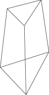
Figure 8. The image of the moment map: the bottom triangle has side length $m\lambda_{1}+\lambda_{2}$, and the top one $\lambda_{2}$.

Figure 9. Invariant 1–dim. subvarieties of the variety ${\mathbb{P}}_{{\mathbb{P}}^{2}}({\mathcal{O}}(m)\oplus 1)$ and their homology classes.

For our calculations of the Gromov–Witten invariants, it will be convenient to have the following weight table at hand, giving the weights of the torus action at the different charts (remember that each maximal cone gives a chart of the toric manifold):

$\sigma_{1}=\langle v_{1},v_{3},v_{4}\rangle$				$\sigma_{4}=\langle v_{2},v_{3},v_{4}\rangle$
$u_{1}$ $=$	$e_{1}^{*}$	${\omega}_{\sigma_{4}}^{\sigma_{1}}$ $=$	${\omega}_{12}-m{\omega}_{5}$	$u_{1}$ $=$	$-e_{1}^{*}$	${\omega}_{\sigma_{1}}^{\sigma_{4}}$ $=$	${\omega}_{21}+m{\omega}_{5}$
$u_{2}$ $=$	$e_{2}^{*}$	${\omega}_{\sigma_{3}}^{\sigma_{1}}$ $=$	${\omega}_{3}-{\omega}_{5}$	$u_{2}$ $=$	$e_{2}^{*}$	${\omega}_{\sigma_{6}}^{\sigma_{4}}$ $=$	${\omega}_{3}-{\omega}_{5}$
$u_{3}$ $=$	$e_{3}^{*}$	${\omega}_{\sigma_{2}}^{\sigma_{1}}$ $=$	${\omega}_{4}-{\omega}_{5}$	$u_{3}$ $=$	$e_{3}^{*}$	${\omega}_{\sigma_{5}}^{\sigma_{4}}$ $=$	${\omega}_{4}-{\omega}_{5}$
$\sigma_{2}=\langle v_{1},v_{3},v_{5}\rangle$				$\sigma_{5}=\langle v_{2},v_{3},v_{5}\rangle$
$u_{1}$ $=$	$e_{1}^{*}-me_{3}^{*}$	${\omega}_{\sigma_{5}}^{\sigma_{2}}$ $=$	${\omega}_{12}-m{\omega}_{4}$	$u_{1}$ $=$	$-e_{1}^{*}+me_{3}^{*}$	${\omega}_{\sigma_{2}}^{\sigma_{5}}$ $=$	${\omega}_{21}+m{\omega}_{4}$
$u_{2}$ $=$	$e_{2}^{*}-e_{3}^{*}$	${\omega}_{\sigma_{3}}^{\sigma_{2}}$ $=$	${\omega}_{3}-{\omega}_{4}$	$u_{2}$ $=$	$e_{2}^{*}-e_{3}^{*}$	${\omega}_{\sigma_{6}}^{\sigma_{5}}$ $=$	${\omega}_{3}-{\omega}_{4}$
$u_{3}$ $=$	$-e_{3}^{*}$	${\omega}_{\sigma_{1}}^{\sigma_{2}}$ $=$	${\omega}_{5}-{\omega}_{4}$	$u_{3}$ $=$	$-e_{3}^{*}$	${\omega}_{\sigma_{4}}^{\sigma_{5}}$ $=$	${\omega}_{5}-{\omega}_{4}$
$\sigma_{3}=\langle v_{1},v_{4},v_{5}\rangle$				$\sigma_{6}=\langle v_{2},v_{4},v_{5}\rangle$
$u_{1}$ $=$	$e_{1}^{*}-me_{2}^{*}$	${\omega}_{\sigma_{6}}^{\sigma_{3}}$ $=$	${\omega}_{12}-m{\omega}_{3}$	$u_{1}$ $=$	$-e_{1}^{*}+me_{2}^{*}$	${\omega}_{\sigma_{3}}^{\sigma_{6}}$ $=$	${\omega}_{21}+m{\omega}_{3}$
$u_{2}$ $=$	$e_{3}^{*}-e_{2}^{*}$	${\omega}_{\sigma_{2}}^{\sigma_{3}}$ $=$	${\omega}_{4}-{\omega}_{3}$	$u_{2}$ $=$	$e_{3}^{*}-e_{2}^{*}$	${\omega}_{\sigma_{5}}^{\sigma_{6}}$ $=$	${\omega}_{4}-{\omega}_{3}$
$u_{3}$ $=$	$-e_{2}^{*}$	${\omega}_{\sigma_{1}}^{\sigma_{3}}$ $=$	${\omega}_{5}-{\omega}_{3}$	$u_{3}$ $=$	$-e_{2}^{*}$	${\omega}_{\sigma_{4}}^{\sigma_{6}}$ $=$	${\omega}_{5}-{\omega}_{3}$

Figure 10. The weight table for ${\mathbb{P}}_{P^{2}}({\mathcal{O}}(m)\oplus 1)$. Substitute ${\omega}_{12}$ by ${\omega}_{1}-{\omega}_{2}$ and ${\omega}_{21}$ by ${\omega}_{2}-{\omega}_{1}$.

9.3. The Gromov–Witten invariants of ${\mathbb{P}}({\mathcal{O}}_{{\mathbb{P}}^{2}}(2)\oplus 1)$

We will now compute all genus–$0$ three–point Gromov–Witten invariants of the Fano threefold ${\mathbb{P}}({\mathcal{O}}_{{\mathbb{P}}^{2}}(2)\oplus 1)$. The Fano property of this manifold implies that there is only a finite number of non–zero invariants.

We will give full details for the computations of some of the invariants, but in some cases, due to the length of the computations, we will just give the different graph types one need to consider and the result. However, even those computations that are omitted here are straightforward.

Remember from above that the degree–$2$ homology classes $\lambda_{1}=(1,1,0,0,0)$ and $\lambda_{2}=(0,-2,1,1,1)$ generate the effective cone. Their pairing with the Chern classes $c_{1}({X_{\Sigma}})$ is two respectively one. Any degree–$2$ homology class $A\in H_{2}({X_{\Sigma}},{\mathbb{Z}})$ having non–zero Gromov–Witten invariants satisfies $\langle c_{1}({X_{\Sigma}}),A\rangle\leq 6$; otherwise the virtual dimension of the moduli stack were negative.

However, it is easy to see that for homology classes $A$ such that $\langle c_{1}({X_{\Sigma}},A\rangle)=6$, all Gromov–Witten invariants are equal to zero: let $A$ be such a class, then the only possibly non–trivial GW invariant would be

$$\Phi^{A}(Z_{1}Z_{3}Z_{4},Z_{1}Z_{3}Z_{5},Z_{1}Z_{4}Z_{5}).$$

However, a graph ${\Gamma}$ such that the integral of these classes over the corresponding fixed point moduli space $\mathcal{M}_{\Gamma}$ is non–zero has to contain the nodes $\sigma_{1}$, $\sigma_{2}$ and $\sigma_{3}$. By looking at figure 9 one immediately sees that such a graph ${\Gamma}$ would have to have homology class $A_{\Gamma}$ with $\langle c_{1}({X_{\Sigma}}),A_{\Gamma}\rangle\geq 8$ (in this case $A_{\Gamma}=3\lambda_{1}+2\lambda_{2}$). Hence, all non–zero Gromov–Witten invariants of ${X_{\Sigma}}$ have $\langle c_{1}({X_{\Sigma}}),A\rangle\leq 5$.

We can equally exclude all classes $A=a_{1}\lambda_{1}+a_{2}\lambda_{2}$ with $a_{2}>3$. For if $\langle c_{1}({X_{\Sigma}}),A\rangle\leq 5$ and $a_{2}>3$ we had $a_{1}=0$. So let us consider the Gromov–Witten invariant

$$\Phi^{a_{2}\lambda_{2}}(\alpha_{1},\alpha_{2},\alpha_{3}).$$

Since $\dim{X_{\Sigma}}=\langle c_{1}({X_{\Sigma}},a_{2}\lambda_{2}\rangle)=3+a_{2}>6$, at least one of the $\alpha_{i}$’s is of degree six, say $\alpha_{1}=Z_{1}Z_{3}Z_{4}$. But there is no graph ${\Gamma}$ of homology class a multiple of $\lambda_{2}$ that contains $\sigma_{1}$.

So we only have to compute the 3–point genus–0 Gromov–Witten invariants for the following classes:

$$\lambda_{2},\lambda_{1},2\lambda_{2},3\lambda_{2},\lambda_{1}+\lambda_{2},2\lambda_{1},\lambda_{1}+2\lambda_{2},\lambda_{1}+3\lambda_{2},2\lambda_{1}+\lambda_{2}.$$

• The graph type for these invariants live on the “upper” triangle in the moment polytope, i.e. they can only contain the vertices $\sigma_{4}$, $\sigma_{5}$ and $\sigma_{6}$.

  • This is because the weight of $Z_{1}$ on the upper triangle is zero.

  • Again, the weight of $Z_{1}$ on the upper triangle is zero, hence the same applies to $Z_{1}Z_{k}$.

  • In this case we get the following two possible graph types:

    $${{\Gamma}_{a}^{\text{type}}}=\mbox{\begin{minipage}[t]{19.91684pt} \begin{center}\rule{0.0pt}{19.91684pt} \huge$\bullet$\\ \parbox{19.91684pt}{\centering\tiny$\sigma_{4}$\@add@centering} \end{center} \end{minipage} }\begin{picture}(10.0,5.0)\put(0.0,1.65){\line(1,0){13.5}} \put(4.0,2.25){\parbox{11.38092pt}{\centering\small 1\@add@centering}} \end{picture}\mbox{\begin{minipage}[t]{19.91684pt} \begin{center}\rule{0.0pt}{19.91684pt} \huge$\bullet$\\ \parbox{19.91684pt}{\centering\tiny$\sigma_{6}$\@add@centering} \end{center} \end{minipage} },\qquad{{\Gamma}_{b}^{\text{type}}}=\mbox{\begin{minipage}[t]{19.91684pt} \begin{center}\rule{0.0pt}{19.91684pt} \huge$\bullet$\\ \parbox{19.91684pt}{\centering\tiny$\sigma_{5}$\@add@centering} \end{center} \end{minipage} }\begin{picture}(10.0,5.0)\put(0.0,1.65){\line(1,0){13.5}} \put(4.0,2.25){\parbox{11.38092pt}{\centering\small 1\@add@centering}} \end{picture}\mbox{\begin{minipage}[t]{19.91684pt} \begin{center}\rule{0.0pt}{19.91684pt} \huge$\bullet$\\ \parbox{19.91684pt}{\centering\tiny$\sigma_{6}$\@add@centering} \end{center} \end{minipage} }.$$

    For both graph types, the automorphism group is trivial. The $S_{{{\Gamma}^{\text{type}}}}$ and $T_{{{\Gamma}^{\text{type}}}}$ terms are as follows:

    $$S_{{{\Gamma}_{a}^{\text{type}}}} =1^{2}\cdot\frac{({\omega}_{4}-{\omega}_{3})({\omega}_{5}-{\omega}_{3})}{({\omega}_{5}-{\omega}_{3})}=({\omega}_{4}-{\omega}_{3})$$

    $$S_{{{\Gamma}_{b}^{\text{type}}}} =1^{2}\cdot\frac{({\omega}_{4}-{\omega}_{3})({\omega}_{5}-{\omega}_{3})}{({\omega}_{4}-{\omega}_{3})}=({\omega}_{5}-{\omega}_{3})$$

    $$T_{{{\Gamma}_{a}^{\text{type}}}} =\frac{(-1)\cdot 1^{2}}{1^{2}({\omega}_{3}-{\omega}_{5})^{2}}\frac{({\omega}_{21}+{\omega}_{3}{\omega}_{5})}{({\omega}_{4}-{\omega}_{5})({\omega}_{4}-{\omega}_{3})}\cdot\frac{({\omega}_{3}-{\omega}_{5})^{2}}{({\omega}_{3}-{\omega}_{5})}\cdot\frac{({\omega}_{5}-{\omega}_{3})^{2}}{({\omega}_{5}-{\omega}_{3})}$$

    $$=\frac{({\omega}_{21}+{\omega}_{3}+{\omega}_{5})}{({\omega}_{4}-{\omega}_{5})({\omega}_{4}-{\omega}_{3})}$$

    $$T_{{{\Gamma}_{b}^{\text{type}}}} =\frac{(-1)\cdot 1^{2}}{1^{2}({\omega}_{3}-{\omega}_{4})^{2}}\frac{(-{\omega}{12}+{\omega}_{3}+{\omega}_{4})}{({\omega}_{5}-{\omega}_{4})({\omega}_{4}-{\omega}_{3})}\cdot\frac{({\omega}_{3}-{\omega}_{4})^{2}}{({\omega}_{3}-{\omega}_{4})}\cdot\frac{({\omega}_{4}-{\omega}_{3})^{2}}{({\omega}_{4}-{\omega}_{3})}$$

    $$=\frac{({\omega}_{21}+{\omega}_{3}+{\omega}_{4})}{({\omega}_{5}-{\omega}_{4})({\omega}_{5}-{\omega}_{3})}$$

• The graph types of this homology class live on the side edges, i.e. either connect $\sigma_{1}$ and $\sigma_{4}$, $\sigma_{2}$ and $\sigma_{5}$, or $\sigma_{3}$ and $\sigma_{6}$.

  • For the weight of $Z_{2}Z_{4}Z_{5}$ not to be zero, the graph has to contain $\sigma_{6}$. However, the weight of $Z_{3}$ at $\sigma_{3}$ and $\sigma_{6}$ is zero.

  • By a similar argument.

  • The only graph type is

    $${{\Gamma}^{\text{type}}}=\mbox{\begin{minipage}[t]{19.91684pt} \begin{center}\rule{0.0pt}{19.91684pt} \huge$\bullet$\\ \parbox{19.91684pt}{\centering\tiny$\sigma_{1}$\@add@centering} \end{center} \end{minipage} }\begin{picture}(10.0,5.0)\put(0.0,1.65){\line(1,0){13.5}} \put(4.0,2.25){\parbox{11.38092pt}{\centering\small 1\@add@centering}} \end{picture}\mbox{\begin{minipage}[t]{19.91684pt} \begin{center}\rule{0.0pt}{19.91684pt} \huge$\bullet$\\ \parbox{19.91684pt}{\centering\tiny$\sigma_{4}$\@add@centering} \end{center} \end{minipage} }$$

    Its automorphism group is trivial, and the two other terms are given by:

    $$S_{{{\Gamma}^{\text{type}}}} =1^{2}\cdot({\omega}_{3}-{\omega}_{5})({\omega}_{4}-{\omega}_{5})$$

    $$T_{{{\Gamma}^{\text{type}}}} =\frac{(-1)}{({\omega}_{12}-2{\omega}_{5})}\frac{1}{({\omega}_{3}-{\omega}_{5})({\omega}_{4}-{\omega}_{5})}\frac{({\omega}_{12}-2{\omega}_{5})^{2}}{({\omega}_{12}-2{\omega}_{5})}\frac{({\omega}_{21}+2{\omega}_{5})^{2}}{({\omega}_{21}+2{\omega}_{5})}.$$

  • We get the same graph type and the same terms $\mathbf{A}_{{{\Gamma}^{\text{type}}}}$, $S_{{{\Gamma}^{\text{type}}}}$ and $T_{{{\Gamma}^{\text{type}}}}$ as in the previous case.

• Again these invariants have to live on the upper $\sigma_{4}$–$\sigma_{5}$–$\sigma_{6}$ triangle of the polytope, so the weight of any class containing $Z_{1}$ will cause an invariant to be zero.

  • The class $\lambda_{2}$ has negative self intersection with the divisor $D_{2}$, hence any holomorphic curve has to lie in $D_{2}$, so it can not pass trough a point in general position.

  • Simply because of $Z_{1}$.

  • Again because of $Z_{1}Z_{j}$.

  • We will just give the graph types one has to consider and leave the actual computations to the reader. The graph types are:

    $${{\Gamma}_{a}^{\text{type}}} =\mbox{\begin{minipage}[t]{19.91684pt} \begin{center}\rule{0.0pt}{19.91684pt} \huge$\bullet$\\ \parbox{19.91684pt}{\centering\tiny$\sigma_{4}$\@add@centering} \end{center} \end{minipage} }\begin{picture}(10.0,5.0)\put(0.0,1.65){\line(1,0){13.5}} \put(4.0,2.25){\parbox{11.38092pt}{\centering\small 2\@add@centering}} \end{picture}\mbox{\begin{minipage}[t]{19.91684pt} \begin{center}\rule{0.0pt}{19.91684pt} \huge$\bullet$\\ \parbox{19.91684pt}{\centering\tiny$\sigma_{6}$\@add@centering} \end{center} \end{minipage} } {{\Gamma}_{b}^{\text{type}}} =\mbox{\begin{minipage}[t]{19.91684pt} \begin{center}\rule{0.0pt}{19.91684pt} \huge$\bullet$\\ \parbox{19.91684pt}{\centering\tiny$\sigma_{4}$\@add@centering} \end{center} \end{minipage} }\begin{picture}(10.0,5.0)\put(0.0,1.65){\line(1,0){13.5}} \put(4.0,2.25){\parbox{11.38092pt}{\centering\small 1\@add@centering}} \end{picture}\mbox{\begin{minipage}[t]{19.91684pt} \begin{center}\rule{0.0pt}{19.91684pt} \huge$\bullet$\\ \parbox{19.91684pt}{\centering\tiny$\sigma_{6}$\@add@centering} \end{center} \end{minipage} }\begin{picture}(10.0,5.0)\put(0.0,1.65){\line(1,0){13.5}} \put(4.0,2.25){\parbox{11.38092pt}{\centering\small 1\@add@centering}} \end{picture}\mbox{\begin{minipage}[t]{19.91684pt} \begin{center}\rule{0.0pt}{19.91684pt} \huge$\bullet$\\ \parbox{19.91684pt}{\centering\tiny$\sigma_{5}$\@add@centering} \end{center} \end{minipage} }$$

    $${{\Gamma}_{aa}^{\text{type}}} =\mbox{\begin{minipage}[t]{19.91684pt} \begin{center}\rule{0.0pt}{19.91684pt} \huge$\bullet$\\ \parbox{19.91684pt}{\centering\tiny$\sigma_{4}$\@add@centering} \end{center} \end{minipage} }\begin{picture}(10.0,5.0)\put(0.0,1.65){\line(1,0){13.5}} \put(4.0,2.25){\parbox{11.38092pt}{\centering\small 1\@add@centering}} \end{picture}\mbox{\begin{minipage}[t]{19.91684pt} \begin{center}\rule{0.0pt}{19.91684pt} \huge$\bullet$\\ \parbox{19.91684pt}{\centering\tiny$\sigma_{6}$\@add@centering} \end{center} \end{minipage} }\begin{picture}(10.0,5.0)\put(0.0,1.65){\line(1,0){13.5}} \put(4.0,2.25){\parbox{11.38092pt}{\centering\small 1\@add@centering}} \end{picture}\mbox{\begin{minipage}[t]{19.91684pt} \begin{center}\rule{0.0pt}{19.91684pt} \huge$\bullet$\\ \parbox{19.91684pt}{\centering\tiny$\sigma_{4}$\@add@centering} \end{center} \end{minipage} } {{\Gamma}_{c}^{\text{type}}} =\mbox{\begin{minipage}[t]{19.91684pt} \begin{center}\rule{0.0pt}{19.91684pt} \huge$\bullet$\\ \parbox{19.91684pt}{\centering\tiny$\sigma_{5}$\@add@centering} \end{center} \end{minipage} }\begin{picture}(10.0,5.0)\put(0.0,1.65){\line(1,0){13.5}} \put(4.0,2.25){\parbox{11.38092pt}{\centering\small 1\@add@centering}} \end{picture}\mbox{\begin{minipage}[t]{19.91684pt} \begin{center}\rule{0.0pt}{19.91684pt} \huge$\bullet$\\ \parbox{19.91684pt}{\centering\tiny$\sigma_{4}$\@add@centering} \end{center} \end{minipage} }\begin{picture}(10.0,5.0)\put(0.0,1.65){\line(1,0){13.5}} \put(4.0,2.25){\parbox{11.38092pt}{\centering\small 1\@add@centering}} \end{picture}\mbox{\begin{minipage}[t]{19.91684pt} \begin{center}\rule{0.0pt}{19.91684pt} \huge$\bullet$\\ \parbox{19.91684pt}{\centering\tiny$\sigma_{6}$\@add@centering} \end{center} \end{minipage} }$$

    $${{\Gamma}_{ab}^{\text{type}}} =\mbox{\begin{minipage}[t]{19.91684pt} \begin{center}\rule{0.0pt}{19.91684pt} \huge$\bullet$\\ \parbox{19.91684pt}{\centering\tiny$\sigma_{6}$\@add@centering} \end{center} \end{minipage} }\begin{picture}(10.0,5.0)\put(0.0,1.65){\line(1,0){13.5}} \put(4.0,2.25){\parbox{11.38092pt}{\centering\small 1\@add@centering}} \end{picture}\mbox{\begin{minipage}[t]{19.91684pt} \begin{center}\rule{0.0pt}{19.91684pt} \huge$\bullet$\\ \parbox{19.91684pt}{\centering\tiny$\sigma_{4}$\@add@centering} \end{center} \end{minipage} }\begin{picture}(10.0,5.0)\put(0.0,1.65){\line(1,0){13.5}} \put(4.0,2.25){\parbox{11.38092pt}{\centering\small 1\@add@centering}} \end{picture}\mbox{\begin{minipage}[t]{19.91684pt} \begin{center}\rule{0.0pt}{19.91684pt} \huge$\bullet$\\ \parbox{19.91684pt}{\centering\tiny$\sigma_{6}$\@add@centering} \end{center} \end{minipage} } {{\Gamma}_{d}^{\text{type}}} =\mbox{\begin{minipage}[t]{19.91684pt} \begin{center}\rule{0.0pt}{19.91684pt} \huge$\bullet$\\ \parbox{19.91684pt}{\centering\tiny$\sigma_{4}$\@add@centering} \end{center} \end{minipage} }\begin{picture}(10.0,5.0)\put(0.0,1.65){\line(1,0){13.5}} \put(4.0,2.25){\parbox{11.38092pt}{\centering\small 1\@add@centering}} \end{picture}\mbox{\begin{minipage}[t]{19.91684pt} \begin{center}\rule{0.0pt}{19.91684pt} \huge$\bullet$\\ \parbox{19.91684pt}{\centering\tiny$\sigma_{5}$\@add@centering} \end{center} \end{minipage} }\begin{picture}(10.0,5.0)\put(0.0,1.65){\line(1,0){13.5}} \put(4.0,2.25){\parbox{11.38092pt}{\centering\small 1\@add@centering}} \end{picture}\mbox{\begin{minipage}[t]{19.91684pt} \begin{center}\rule{0.0pt}{19.91684pt} \huge$\bullet$\\ \parbox{19.91684pt}{\centering\tiny$\sigma_{6}$\@add@centering} \end{center} \end{minipage} }$$

• Again, all graphs have to live on the upper triangle of the polytope. Therefore we get:

  • Because of the $Z_{1}$ in the third class.

  • Because of the $Z_{1}$ in the first class.

  • Again, we only give the different graph types here — they are:

    $${{\Gamma}_{a}^{\text{type}}} =\mbox{\begin{minipage}[t]{19.91684pt} \begin{center}\rule{0.0pt}{19.91684pt} \huge$\bullet$\\ \parbox{19.91684pt}{\centering\tiny$\sigma_{5}$\@add@centering} \end{center} \end{minipage} }\begin{picture}(10.0,5.0)\put(0.0,1.65){\line(1,0){13.5}} \put(4.0,2.25){\parbox{11.38092pt}{\centering\small 2\@add@centering}} \end{picture}\mbox{\begin{minipage}[t]{19.91684pt} \begin{center}\rule{0.0pt}{19.91684pt} \huge$\bullet$\\ \parbox{19.91684pt}{\centering\tiny$\sigma_{4}$\@add@centering} \end{center} \end{minipage} }\begin{picture}(10.0,5.0)\put(0.0,1.65){\line(1,0){13.5}} \put(4.0,2.25){\parbox{11.38092pt}{\centering\small 1\@add@centering}} \end{picture}\mbox{\begin{minipage}[t]{19.91684pt} \begin{center}\rule{0.0pt}{19.91684pt} \huge$\bullet$\\ \parbox{19.91684pt}{\centering\tiny$\sigma_{6}$\@add@centering} \end{center} \end{minipage} } {{\Gamma}_{b}^{\text{type}}} =\mbox{\begin{minipage}[t]{19.91684pt} \begin{center}\rule{0.0pt}{19.91684pt} \huge$\bullet$\\ \parbox{19.91684pt}{\centering\tiny$\sigma_{5}$\@add@centering} \end{center} \end{minipage} }\begin{picture}(10.0,5.0)\put(0.0,1.65){\line(1,0){13.5}} \put(4.0,2.25){\parbox{11.38092pt}{\centering\small 1\@add@centering}} \end{picture}\mbox{\begin{minipage}[t]{19.91684pt} \begin{center}\rule{0.0pt}{19.91684pt} \huge$\bullet$\\ \parbox{19.91684pt}{\centering\tiny$\sigma_{4}$\@add@centering} \end{center} \end{minipage} }\begin{picture}(10.0,5.0)\put(0.0,1.65){\line(1,0){13.5}} \put(4.0,2.25){\parbox{11.38092pt}{\centering\small 2\@add@centering}} \end{picture}\mbox{\begin{minipage}[t]{19.91684pt} \begin{center}\rule{0.0pt}{19.91684pt} \huge$\bullet$\\ \parbox{19.91684pt}{\centering\tiny$\sigma_{6}$\@add@centering} \end{center} \end{minipage} }$$

    $${{\Gamma}_{aa}^{\text{type}}} =\mbox{\begin{minipage}[t]{19.91684pt} \begin{center}\rule{0.0pt}{19.91684pt} \huge$\bullet$\\ \parbox{19.91684pt}{\centering\tiny$\sigma_{4}$\@add@centering} \end{center} \end{minipage} }\begin{picture}(6.0,5.0)\put(0.0,1.65){\line(1,0){9.5}} \put(2.0,2.25){\parbox{11.38092pt}{\centering\small 1\@add@centering}} \end{picture}\mbox{\begin{minipage}[t]{19.91684pt} \begin{center}\rule{0.0pt}{19.91684pt} \huge$\bullet$\\ \parbox{19.91684pt}{\centering\tiny$\sigma_{5}$\@add@centering} \end{center} \end{minipage} }\begin{picture}(6.0,5.0)\put(0.0,1.65){\line(1,0){9.5}} \put(2.0,2.25){\parbox{11.38092pt}{\centering\small 1\@add@centering}} \end{picture}\mbox{\begin{minipage}[t]{19.91684pt} \begin{center}\rule{0.0pt}{19.91684pt} \huge$\bullet$\\ \parbox{19.91684pt}{\centering\tiny$\sigma_{4}$\@add@centering} \end{center} \end{minipage} }\begin{picture}(6.0,5.0)\put(0.0,1.65){\line(1,0){9.5}} \put(2.0,2.25){\parbox{11.38092pt}{\centering\small 1\@add@centering}} \end{picture}\mbox{\begin{minipage}[t]{19.91684pt} \begin{center}\rule{0.0pt}{19.91684pt} \huge$\bullet$\\ \parbox{19.91684pt}{\centering\tiny$\sigma_{6}$\@add@centering} \end{center} \end{minipage} } {{\Gamma}_{ba}^{\text{type}}} =\mbox{\begin{minipage}[t]{19.91684pt} \begin{center}\rule{0.0pt}{19.91684pt} \huge$\bullet$\\ \parbox{19.91684pt}{\centering\tiny$\sigma_{4}$\@add@centering} \end{center} \end{minipage} }\begin{picture}(6.0,5.0)\put(0.0,1.65){\line(1,0){9.5}} \put(2.0,2.25){\parbox{11.38092pt}{\centering\small 1\@add@centering}} \end{picture}\mbox{\begin{minipage}[t]{19.91684pt} \begin{center}\rule{0.0pt}{19.91684pt} \huge$\bullet$\\ \parbox{19.91684pt}{\centering\tiny$\sigma_{6}$\@add@centering} \end{center} \end{minipage} }\begin{picture}(6.0,5.0)\put(0.0,1.65){\line(1,0){9.5}} \put(2.0,2.25){\parbox{11.38092pt}{\centering\small 1\@add@centering}} \end{picture}\mbox{\begin{minipage}[t]{19.91684pt} \begin{center}\rule{0.0pt}{19.91684pt} \huge$\bullet$\\ \parbox{19.91684pt}{\centering\tiny$\sigma_{5}$\@add@centering} \end{center} \end{minipage} }\begin{picture}(6.0,5.0)\put(0.0,1.65){\line(1,0){9.5}} \put(2.0,2.25){\parbox{11.38092pt}{\centering\small 1\@add@centering}} \end{picture}\mbox{\begin{minipage}[t]{19.91684pt} \begin{center}\rule{0.0pt}{19.91684pt} \huge$\bullet$\\ \parbox{19.91684pt}{\centering\tiny$\sigma_{4}$\@add@centering} \end{center} \end{minipage} }$$

    $${{\Gamma}_{ab}^{\text{type}}} =\mbox{\begin{picture}(33.0,16.0)\put(0.0,0.0){\mbox{\begin{minipage}[t]{19.91684pt} \begin{center}\rule{0.0pt}{19.91684pt} \huge$\bullet$\\ \parbox{19.91684pt}{\centering\tiny$\sigma_{5}$\@add@centering} \end{center} \end{minipage} } } \put(13.0,0.0){\mbox{\begin{minipage}[t]{19.91684pt} \begin{center}\rule{0.0pt}{19.91684pt} \huge$\bullet$\\ \parbox{19.91684pt}{\centering\tiny$\sigma_{4}$\@add@centering} \end{center} \end{minipage} } } \put(26.0,0.0){\mbox{\begin{minipage}[t]{19.91684pt} \begin{center}\rule{0.0pt}{19.91684pt} \huge$\bullet$\\ \parbox{19.91684pt}{\centering\tiny$\sigma_{6}$\@add@centering} \end{center} \end{minipage} } } \put(12.0,13.0){ \mbox{\begin{minipage}[t]{19.91684pt} \begin{center}\rule{0.0pt}{19.91684pt} \huge$\bullet$\\ \parbox{19.91684pt}{\hfill\tiny$\sigma_{5}$} \end{center} \end{minipage} } } \put(3.5,1.5){\line(1,0){26.0}} \put(16.5,0.0){\line(0,1){13.5}} \end{picture} } {{\Gamma}_{bb}^{\text{type}}} =\mbox{\begin{picture}(33.0,16.0)\put(0.0,0.0){\mbox{\begin{minipage}[t]{19.91684pt} \begin{center}\rule{0.0pt}{19.91684pt} \huge$\bullet$\\ \parbox{19.91684pt}{\centering\tiny$\sigma_{5}$\@add@centering} \end{center} \end{minipage} } } \put(13.0,0.0){\mbox{\begin{minipage}[t]{19.91684pt} \begin{center}\rule{0.0pt}{19.91684pt} \huge$\bullet$\\ \parbox{19.91684pt}{\centering\tiny$\sigma_{4}$\@add@centering} \end{center} \end{minipage} } } \put(26.0,0.0){\mbox{\begin{minipage}[t]{19.91684pt} \begin{center}\rule{0.0pt}{19.91684pt} \huge$\bullet$\\ \parbox{19.91684pt}{\centering\tiny$\sigma_{6}$\@add@centering} \end{center} \end{minipage} } } \put(12.0,13.0){ \mbox{\begin{minipage}[t]{19.91684pt} \begin{center}\rule{0.0pt}{19.91684pt} \huge$\bullet$\\ \parbox{19.91684pt}{\hfill\tiny$\sigma_{5}$} \end{center} \end{minipage} } } \put(3.5,1.5){\line(1,0){26.0}} \put(16.5,0.0){\line(0,1){13.5}} \end{picture} }$$

    $${{\Gamma}_{c}^{\text{type}}} =\mbox{\begin{minipage}[t]{19.91684pt} \begin{center}\rule{0.0pt}{19.91684pt} \huge$\bullet$\\ \parbox{19.91684pt}{\centering\tiny$\sigma_{4}$\@add@centering} \end{center} \end{minipage} }\begin{picture}(10.0,5.0)\put(0.0,1.65){\line(1,0){13.5}} \put(4.0,2.25){\parbox{11.38092pt}{\centering\small 2\@add@centering}} \end{picture}\mbox{\begin{minipage}[t]{19.91684pt} \begin{center}\rule{0.0pt}{19.91684pt} \huge$\bullet$\\ \parbox{19.91684pt}{\centering\tiny$\sigma_{5}$\@add@centering} \end{center} \end{minipage} }\begin{picture}(10.0,5.0)\put(0.0,1.65){\line(1,0){13.5}} \put(4.0,2.25){\parbox{11.38092pt}{\centering\small 1\@add@centering}} \end{picture}\mbox{\begin{minipage}[t]{19.91684pt} \begin{center}\rule{0.0pt}{19.91684pt} \huge$\bullet$\\ \parbox{19.91684pt}{\centering\tiny$\sigma_{6}$\@add@centering} \end{center} \end{minipage} } {{\Gamma}_{d}^{\text{type}}} =\mbox{\begin{minipage}[t]{19.91684pt} \begin{center}\rule{0.0pt}{19.91684pt} \huge$\bullet$\\ \parbox{19.91684pt}{\centering\tiny$\sigma_{4}$\@add@centering} \end{center} \end{minipage} }\begin{picture}(10.0,5.0)\put(0.0,1.65){\line(1,0){13.5}} \put(4.0,2.25){\parbox{11.38092pt}{\centering\small 1\@add@centering}} \end{picture}\mbox{\begin{minipage}[t]{19.91684pt} \begin{center}\rule{0.0pt}{19.91684pt} \huge$\bullet$\\ \parbox{19.91684pt}{\centering\tiny$\sigma_{5}$\@add@centering} \end{center} \end{minipage} }\begin{picture}(10.0,5.0)\put(0.0,1.65){\line(1,0){13.5}} \put(4.0,2.25){\parbox{11.38092pt}{\centering\small 2\@add@centering}} \end{picture}\mbox{\begin{minipage}[t]{19.91684pt} \begin{center}\rule{0.0pt}{19.91684pt} \huge$\bullet$\\ \parbox{19.91684pt}{\centering\tiny$\sigma_{6}$\@add@centering} \end{center} \end{minipage} }$$

    $${{\Gamma}_{ca}^{\text{type}}} =\mbox{\begin{minipage}[t]{19.91684pt} \begin{center}\rule{0.0pt}{19.91684pt} \huge$\bullet$\\ \parbox{19.91684pt}{\centering\tiny$\sigma_{5}$\@add@centering} \end{center} \end{minipage} }\begin{picture}(6.0,5.0)\put(0.0,1.65){\line(1,0){9.5}} \put(2.0,2.25){\parbox{11.38092pt}{\centering\small 1\@add@centering}} \end{picture}\mbox{\begin{minipage}[t]{19.91684pt} \begin{center}\rule{0.0pt}{19.91684pt} \huge$\bullet$\\ \parbox{19.91684pt}{\centering\tiny$\sigma_{4}$\@add@centering} \end{center} \end{minipage} }\begin{picture}(6.0,5.0)\put(0.0,1.65){\line(1,0){9.5}} \put(2.0,2.25){\parbox{11.38092pt}{\centering\small 1\@add@centering}} \end{picture}\mbox{\begin{minipage}[t]{19.91684pt} \begin{center}\rule{0.0pt}{19.91684pt} \huge$\bullet$\\ \parbox{19.91684pt}{\centering\tiny$\sigma_{5}$\@add@centering} \end{center} \end{minipage} }\begin{picture}(6.0,5.0)\put(0.0,1.65){\line(1,0){9.5}} \put(2.0,2.25){\parbox{11.38092pt}{\centering\small 1\@add@centering}} \end{picture}\mbox{\begin{minipage}[t]{19.91684pt} \begin{center}\rule{0.0pt}{19.91684pt} \huge$\bullet$\\ \parbox{19.91684pt}{\centering\tiny$\sigma_{6}$\@add@centering} \end{center} \end{minipage} } {{\Gamma}_{da}^{\text{type}}} =\mbox{\begin{minipage}[t]{19.91684pt} \begin{center}\rule{0.0pt}{19.91684pt} \huge$\bullet$\\ \parbox{19.91684pt}{\centering\tiny$\sigma_{4}$\@add@centering} \end{center} \end{minipage} }\begin{picture}(6.0,5.0)\put(0.0,1.65){\line(1,0){9.5}} \put(2.0,2.25){\parbox{11.38092pt}{\centering\small 1\@add@centering}} \end{picture}\mbox{\begin{minipage}[t]{19.91684pt} \begin{center}\rule{0.0pt}{19.91684pt} \huge$\bullet$\\ \parbox{19.91684pt}{\centering\tiny$\sigma_{5}$\@add@centering} \end{center} \end{minipage} }\begin{picture}(6.0,5.0)\put(0.0,1.65){\line(1,0){9.5}} \put(2.0,2.25){\parbox{11.38092pt}{\centering\small 1\@add@centering}} \end{picture}\mbox{\begin{minipage}[t]{19.91684pt} \begin{center}\rule{0.0pt}{19.91684pt} \huge$\bullet$\\ \parbox{19.91684pt}{\centering\tiny$\sigma_{6}$\@add@centering} \end{center} \end{minipage} }\begin{picture}(6.0,5.0)\put(0.0,1.65){\line(1,0){9.5}} \put(2.0,2.25){\parbox{11.38092pt}{\centering\small 1\@add@centering}} \end{picture}\mbox{\begin{minipage}[t]{19.91684pt} \begin{center}\rule{0.0pt}{19.91684pt} \huge$\bullet$\\ \parbox{19.91684pt}{\centering\tiny$\sigma_{5}$\@add@centering} \end{center} \end{minipage} }$$

    $${{\Gamma}_{cb}^{\text{type}}} =\mbox{\begin{picture}(33.0,16.0)\put(0.0,0.0){\mbox{\begin{minipage}[t]{19.91684pt} \begin{center}\rule{0.0pt}{19.91684pt} \huge$\bullet$\\ \parbox{19.91684pt}{\centering\tiny$\sigma_{4}$\@add@centering} \end{center} \end{minipage} } } \put(13.0,0.0){\mbox{\begin{minipage}[t]{19.91684pt} \begin{center}\rule{0.0pt}{19.91684pt} \huge$\bullet$\\ \parbox{19.91684pt}{\centering\tiny$\sigma_{5}$\@add@centering} \end{center} \end{minipage} } } \put(26.0,0.0){\mbox{\begin{minipage}[t]{19.91684pt} \begin{center}\rule{0.0pt}{19.91684pt} \huge$\bullet$\\ \parbox{19.91684pt}{\centering\tiny$\sigma_{6}$\@add@centering} \end{center} \end{minipage} } } \put(12.0,13.0){ \mbox{\begin{minipage}[t]{19.91684pt} \begin{center}\rule{0.0pt}{19.91684pt} \huge$\bullet$\\ \parbox{19.91684pt}{\hfill\tiny$\sigma_{4}$} \end{center} \end{minipage} } } \put(3.5,1.5){\line(1,0){26.0}} \put(16.5,0.0){\line(0,1){13.5}} \end{picture} } {{\Gamma}_{db}^{\text{type}}} =\mbox{\begin{picture}(33.0,16.0)\put(0.0,0.0){\mbox{\begin{minipage}[t]{19.91684pt} \begin{center}\rule{0.0pt}{19.91684pt} \huge$\bullet$\\ \parbox{19.91684pt}{\centering\tiny$\sigma_{4}$\@add@centering} \end{center} \end{minipage} } } \put(13.0,0.0){\mbox{\begin{minipage}[t]{19.91684pt} \begin{center}\rule{0.0pt}{19.91684pt} \huge$\bullet$\\ \parbox{19.91684pt}{\centering\tiny$\sigma_{5}$\@add@centering} \end{center} \end{minipage} } } \put(26.0,0.0){\mbox{\begin{minipage}[t]{19.91684pt} \begin{center}\rule{0.0pt}{19.91684pt} \huge$\bullet$\\ \parbox{19.91684pt}{\centering\tiny$\sigma_{6}$\@add@centering} \end{center} \end{minipage} } } \put(12.0,13.0){ \mbox{\begin{minipage}[t]{19.91684pt} \begin{center}\rule{0.0pt}{19.91684pt} \huge$\bullet$\\ \parbox{19.91684pt}{\hfill\tiny$\sigma_{4}$} \end{center} \end{minipage} } } \put(3.5,1.5){\line(1,0){26.0}} \put(16.5,0.0){\line(0,1){13.5}} \end{picture} }$$

    $${{\Gamma}_{e}^{\text{type}}} =\mbox{\begin{minipage}[t]{19.91684pt} \begin{center}\rule{0.0pt}{19.91684pt} \huge$\bullet$\\ \parbox{19.91684pt}{\centering\tiny$\sigma_{4}$\@add@centering} \end{center} \end{minipage} }\begin{picture}(10.0,5.0)\put(0.0,1.65){\line(1,0){13.5}} \put(4.0,2.25){\parbox{11.38092pt}{\centering\small 2\@add@centering}} \end{picture}\mbox{\begin{minipage}[t]{19.91684pt} \begin{center}\rule{0.0pt}{19.91684pt} \huge$\bullet$\\ \parbox{19.91684pt}{\centering\tiny$\sigma_{6}$\@add@centering} \end{center} \end{minipage} }\begin{picture}(10.0,5.0)\put(0.0,1.65){\line(1,0){13.5}} \put(4.0,2.25){\parbox{11.38092pt}{\centering\small 1\@add@centering}} \end{picture}\mbox{\begin{minipage}[t]{19.91684pt} \begin{center}\rule{0.0pt}{19.91684pt} \huge$\bullet$\\ \parbox{19.91684pt}{\centering\tiny$\sigma_{5}$\@add@centering} \end{center} \end{minipage} } {{\Gamma}_{f}^{\text{type}}} =\mbox{\begin{minipage}[t]{19.91684pt} \begin{center}\rule{0.0pt}{19.91684pt} \huge$\bullet$\\ \parbox{19.91684pt}{\centering\tiny$\sigma_{4}$\@add@centering} \end{center} \end{minipage} }\begin{picture}(10.0,5.0)\put(0.0,1.65){\line(1,0){13.5}} \put(4.0,2.25){\parbox{11.38092pt}{\centering\small 1\@add@centering}} \end{picture}\mbox{\begin{minipage}[t]{19.91684pt} \begin{center}\rule{0.0pt}{19.91684pt} \huge$\bullet$\\ \parbox{19.91684pt}{\centering\tiny$\sigma_{6}$\@add@centering} \end{center} \end{minipage} }\begin{picture}(10.0,5.0)\put(0.0,1.65){\line(1,0){13.5}} \put(4.0,2.25){\parbox{11.38092pt}{\centering\small 2\@add@centering}} \end{picture}\mbox{\begin{minipage}[t]{19.91684pt} \begin{center}\rule{0.0pt}{19.91684pt} \huge$\bullet$\\ \parbox{19.91684pt}{\centering\tiny$\sigma_{5}$\@add@centering} \end{center} \end{minipage} }$$

    $${{\Gamma}_{ea}^{\text{type}}} =\mbox{\begin{minipage}[t]{19.91684pt} \begin{center}\rule{0.0pt}{19.91684pt} \huge$\bullet$\\ \parbox{19.91684pt}{\centering\tiny$\sigma_{6}$\@add@centering} \end{center} \end{minipage} }\begin{picture}(6.0,5.0)\put(0.0,1.65){\line(1,0){9.5}} \put(2.0,2.25){\parbox{11.38092pt}{\centering\small 1\@add@centering}} \end{picture}\mbox{\begin{minipage}[t]{19.91684pt} \begin{center}\rule{0.0pt}{19.91684pt} \huge$\bullet$\\ \parbox{19.91684pt}{\centering\tiny$\sigma_{4}$\@add@centering} \end{center} \end{minipage} }\begin{picture}(6.0,5.0)\put(0.0,1.65){\line(1,0){9.5}} \put(2.0,2.25){\parbox{11.38092pt}{\centering\small 1\@add@centering}} \end{picture}\mbox{\begin{minipage}[t]{19.91684pt} \begin{center}\rule{0.0pt}{19.91684pt} \huge$\bullet$\\ \parbox{19.91684pt}{\centering\tiny$\sigma_{6}$\@add@centering} \end{center} \end{minipage} }\begin{picture}(6.0,5.0)\put(0.0,1.65){\line(1,0){9.5}} \put(2.0,2.25){\parbox{11.38092pt}{\centering\small 1\@add@centering}} \end{picture}\mbox{\begin{minipage}[t]{19.91684pt} \begin{center}\rule{0.0pt}{19.91684pt} \huge$\bullet$\\ \parbox{19.91684pt}{\centering\tiny$\sigma_{5}$\@add@centering} \end{center} \end{minipage} } {{\Gamma}_{fa}^{\text{type}}} =\mbox{\begin{minipage}[t]{19.91684pt} \begin{center}\rule{0.0pt}{19.91684pt} \huge$\bullet$\\ \parbox{19.91684pt}{\centering\tiny$\sigma_{4}$\@add@centering} \end{center} \end{minipage} }\begin{picture}(6.0,5.0)\put(0.0,1.65){\line(1,0){9.5}} \put(2.0,2.25){\parbox{11.38092pt}{\centering\small 1\@add@centering}} \end{picture}\mbox{\begin{minipage}[t]{19.91684pt} \begin{center}\rule{0.0pt}{19.91684pt} \huge$\bullet$\\ \parbox{19.91684pt}{\centering\tiny$\sigma_{6}$\@add@centering} \end{center} \end{minipage} }\begin{picture}(6.0,5.0)\put(0.0,1.65){\line(1,0){9.5}} \put(2.0,2.25){\parbox{11.38092pt}{\centering\small 1\@add@centering}} \end{picture}\mbox{\begin{minipage}[t]{19.91684pt} \begin{center}\rule{0.0pt}{19.91684pt} \huge$\bullet$\\ \parbox{19.91684pt}{\centering\tiny$\sigma_{5}$\@add@centering} \end{center} \end{minipage} }\begin{picture}(6.0,5.0)\put(0.0,1.65){\line(1,0){9.5}} \put(2.0,2.25){\parbox{11.38092pt}{\centering\small 1\@add@centering}} \end{picture}\mbox{\begin{minipage}[t]{19.91684pt} \begin{center}\rule{0.0pt}{19.91684pt} \huge$\bullet$\\ \parbox{19.91684pt}{\centering\tiny$\sigma_{6}$\@add@centering} \end{center} \end{minipage} }$$

    $${{\Gamma}_{eb}^{\text{type}}} =\mbox{\begin{picture}(33.0,16.0)\put(0.0,0.0){\mbox{\begin{minipage}[t]{19.91684pt} \begin{center}\rule{0.0pt}{19.91684pt} \huge$\bullet$\\ \parbox{19.91684pt}{\centering\tiny$\sigma_{4}$\@add@centering} \end{center} \end{minipage} } } \put(13.0,0.0){\mbox{\begin{minipage}[t]{19.91684pt} \begin{center}\rule{0.0pt}{19.91684pt} \huge$\bullet$\\ \parbox{19.91684pt}{\centering\tiny$\sigma_{6}$\@add@centering} \end{center} \end{minipage} } } \put(26.0,0.0){\mbox{\begin{minipage}[t]{19.91684pt} \begin{center}\rule{0.0pt}{19.91684pt} \huge$\bullet$\\ \parbox{19.91684pt}{\centering\tiny$\sigma_{5}$\@add@centering} \end{center} \end{minipage} } } \put(12.0,13.0){ \mbox{\begin{minipage}[t]{19.91684pt} \begin{center}\rule{0.0pt}{19.91684pt} \huge$\bullet$\\ \parbox{19.91684pt}{\hfill\tiny$\sigma_{4}$} \end{center} \end{minipage} } } \put(3.5,1.5){\line(1,0){26.0}} \put(16.5,0.0){\line(0,1){13.5}} \end{picture} } {{\Gamma}_{fb}^{\text{type}}} =\mbox{\begin{picture}(33.0,16.0)\put(0.0,0.0){\mbox{\begin{minipage}[t]{19.91684pt} \begin{center}\rule{0.0pt}{19.91684pt} \huge$\bullet$\\ \parbox{19.91684pt}{\centering\tiny$\sigma_{4}$\@add@centering} \end{center} \end{minipage} } } \put(13.0,0.0){\mbox{\begin{minipage}[t]{19.91684pt} \begin{center}\rule{0.0pt}{19.91684pt} \huge$\bullet$\\ \parbox{19.91684pt}{\centering\tiny$\sigma_{5}$\@add@centering} \end{center} \end{minipage} } } \put(26.0,0.0){\mbox{\begin{minipage}[t]{19.91684pt} \begin{center}\rule{0.0pt}{19.91684pt} \huge$\bullet$\\ \parbox{19.91684pt}{\centering\tiny$\sigma_{5}$\@add@centering} \end{center} \end{minipage} } } \put(12.0,13.0){ \mbox{\begin{minipage}[t]{19.91684pt} \begin{center}\rule{0.0pt}{19.91684pt} \huge$\bullet$\\ \parbox{19.91684pt}{\hfill\tiny$\sigma_{4}$} \end{center} \end{minipage} } } \put(3.5,1.5){\line(1,0){26.0}} \put(16.5,0.0){\line(0,1){13.5}} \end{picture} }$$

    $${{\Gamma}_{ga}^{\text{type}}} =\mbox{\begin{minipage}[t]{19.91684pt} \begin{center}\rule{0.0pt}{19.91684pt} \huge$\bullet$\\ \parbox{19.91684pt}{\centering\tiny$\sigma_{4}$\@add@centering} \end{center} \end{minipage} }\begin{picture}(6.0,5.0)\put(0.0,1.65){\line(1,0){9.5}} \put(2.0,2.25){\parbox{11.38092pt}{\centering\small 1\@add@centering}} \end{picture}\mbox{\begin{minipage}[t]{19.91684pt} \begin{center}\rule{0.0pt}{19.91684pt} \huge$\bullet$\\ \parbox{19.91684pt}{\centering\tiny$\sigma_{5}$\@add@centering} \end{center} \end{minipage} }\begin{picture}(6.0,5.0)\put(0.0,1.65){\line(1,0){9.5}} \put(2.0,2.25){\parbox{11.38092pt}{\centering\small 1\@add@centering}} \end{picture}\mbox{\begin{minipage}[t]{19.91684pt} \begin{center}\rule{0.0pt}{19.91684pt} \huge$\bullet$\\ \parbox{19.91684pt}{\centering\tiny$\sigma_{6}$\@add@centering} \end{center} \end{minipage} }\begin{picture}(6.0,5.0)\put(0.0,1.65){\line(1,0){9.5}} \put(2.0,2.25){\parbox{11.38092pt}{\centering\small 1\@add@centering}} \end{picture}\mbox{\begin{minipage}[t]{19.91684pt} \begin{center}\rule{0.0pt}{19.91684pt} \huge$\bullet$\\ \parbox{19.91684pt}{\centering\tiny$\sigma_{4}$\@add@centering} \end{center} \end{minipage} } {{\Gamma}_{gb}^{\text{type}}} =\mbox{\begin{minipage}[t]{19.91684pt} \begin{center}\rule{0.0pt}{19.91684pt} \huge$\bullet$\\ \parbox{19.91684pt}{\centering\tiny$\sigma_{5}$\@add@centering} \end{center} \end{minipage} }\begin{picture}(6.0,5.0)\put(0.0,1.65){\line(1,0){9.5}} \put(2.0,2.25){\parbox{11.38092pt}{\centering\small 1\@add@centering}} \end{picture}\mbox{\begin{minipage}[t]{19.91684pt} \begin{center}\rule{0.0pt}{19.91684pt} \huge$\bullet$\\ \parbox{19.91684pt}{\centering\tiny$\sigma_{4}$\@add@centering} \end{center} \end{minipage} }\begin{picture}(6.0,5.0)\put(0.0,1.65){\line(1,0){9.5}} \put(2.0,2.25){\parbox{11.38092pt}{\centering\small 1\@add@centering}} \end{picture}\mbox{\begin{minipage}[t]{19.91684pt} \begin{center}\rule{0.0pt}{19.91684pt} \huge$\bullet$\\ \parbox{19.91684pt}{\centering\tiny$\sigma_{6}$\@add@centering} \end{center} \end{minipage} }\begin{picture}(6.0,5.0)\put(0.0,1.65){\line(1,0){9.5}} \put(2.0,2.25){\parbox{11.38092pt}{\centering\small 1\@add@centering}} \end{picture}\mbox{\begin{minipage}[t]{19.91684pt} \begin{center}\rule{0.0pt}{19.91684pt} \huge$\bullet$\\ \parbox{19.91684pt}{\centering\tiny$\sigma_{5}$\@add@centering} \end{center} \end{minipage} }$$

    $${{\Gamma}_{gc}^{\text{type}}} =\mbox{\begin{minipage}[t]{19.91684pt} \begin{center}\rule{0.0pt}{19.91684pt} \huge$\bullet$\\ \parbox{19.91684pt}{\centering\tiny$\sigma_{6}$\@add@centering} \end{center} \end{minipage} }\begin{picture}(6.0,5.0)\put(0.0,1.65){\line(1,0){9.5}} \put(2.0,2.25){\parbox{11.38092pt}{\centering\small 1\@add@centering}} \end{picture}\mbox{\begin{minipage}[t]{19.91684pt} \begin{center}\rule{0.0pt}{19.91684pt} \huge$\bullet$\\ \parbox{19.91684pt}{\centering\tiny$\sigma_{4}$\@add@centering} \end{center} \end{minipage} }\begin{picture}(6.0,5.0)\put(0.0,1.65){\line(1,0){9.5}} \put(2.0,2.25){\parbox{11.38092pt}{\centering\small 1\@add@centering}} \end{picture}\mbox{\begin{minipage}[t]{19.91684pt} \begin{center}\rule{0.0pt}{19.91684pt} \huge$\bullet$\\ \parbox{19.91684pt}{\centering\tiny$\sigma_{5}$\@add@centering} \end{center} \end{minipage} }\begin{picture}(6.0,5.0)\put(0.0,1.65){\line(1,0){9.5}} \put(2.0,2.25){\parbox{11.38092pt}{\centering\small 1\@add@centering}} \end{picture}\mbox{\begin{minipage}[t]{19.91684pt} \begin{center}\rule{0.0pt}{19.91684pt} \huge$\bullet$\\ \parbox{19.91684pt}{\centering\tiny$\sigma_{6}$\@add@centering} \end{center} \end{minipage} }$$

• The graph types have one component in the upper triangle and one on a side edge — they can not have an edge on the lower triangle $\sigma_{1}$–$\sigma_{2}$–$\sigma_{3}$.

  • The third marked point has to be at $\sigma_{1}$, and the second at $\sigma_{2}$ or $\sigma_{3}$ which would require an edge on the lower triangle.

  • Needs two edges in the upper triangle.

  • Needs an edge in the lower triangle.

  • The only graph type to consider is

    $${{\Gamma}^{\text{type}}}=\mbox{\begin{minipage}[t]{19.91684pt} \begin{center}\rule{0.0pt}{19.91684pt} \huge$\bullet$\\ \parbox{19.91684pt}{\centering\tiny$\sigma_{1}$\@add@centering} \end{center} \end{minipage} }\begin{picture}(10.0,5.0)\put(0.0,1.65){\line(1,0){13.5}} \put(4.0,2.25){\parbox{11.38092pt}{\centering\small 1\@add@centering}} \end{picture}\mbox{\begin{minipage}[t]{19.91684pt} \begin{center}\rule{0.0pt}{19.91684pt} \huge$\bullet$\\ \parbox{19.91684pt}{\centering\tiny$\sigma_{4}$\@add@centering} \end{center} \end{minipage} }\begin{picture}(10.0,5.0)\put(0.0,1.65){\line(1,0){13.5}} \put(4.0,2.25){\parbox{11.38092pt}{\centering\small 1\@add@centering}} \end{picture}\mbox{\begin{minipage}[t]{19.91684pt} \begin{center}\rule{0.0pt}{19.91684pt} \huge$\bullet$\\ \parbox{19.91684pt}{\centering\tiny$\sigma_{6}$\@add@centering} \end{center} \end{minipage} }$$

    The automorphism group is trivial, $S_{{{\Gamma}^{\text{type}}}}=({\omega}_{4}-{\omega}_{3})({\omega}_{3}-{\omega}_{5})({\omega}_{4}-{\omega}_{5})$, and $T_{{{\Gamma}^{\text{type}}}}$ the invers of $S_{{{\Gamma}^{\text{type}}}}$.

  • Same graph and terms as in the previous case.

  • Again the same.

  • Again the same.

• The virtual dimension of the corresponding moduli space is seven, so for the invariants $\Phi^{2\lambda_{1}}(\alpha_{1},\alpha_{2},\alpha_{3})$ we have two cases for the classes $\alpha_{i}$:

  • $\deg\alpha_{1}=\deg\alpha_{2}=6$ and $\deg\alpha_{3}=2$
    In this cases we can set $\alpha_{1}=Z_{1}Z_{3}Z_{4}$ and $\alpha_{2}=Z_{1}Z_{4}Z_{5}$. There is obviously no graph ${\Gamma}$ in the homology class $2\lambda_{1}$ containing both $\sigma_{1}$ and $\sigma_{3}$.

  • $\deg\alpha_{1}=6$ and $\deg\alpha_{2}=\deg\alpha_{3}=4$
    We can set $\alpha_{1}=Z_{1}Z_{3}Z_{4}$. For $\alpha_{2}$ we have to choices: $\alpha_{2}=Z_{4}Z_{5}$ or $\alpha_{2}=Z_{1}Z_{5}$. Again, there is no graph ${\Gamma}$ with homology class $2\lambda_{1}$ that contains the necessary nodes ($\sigma_{1}$ and one of the following: $\sigma_{3}$ or $\sigma_{6}$ respectively $\sigma_{2}$ or $\sigma_{3}$).

• Since the homology class $A=\lambda_{1}+2\lambda_{2}$ contains only one $\lambda_{1}$, all graphs ${\Gamma}$ in this homology class contain exactly one of the following nodes: $\sigma_{1}$, $\sigma_{2}$ and $\sigma_{3}$. Therefore the following invariants are all zero:

  Only Gromov–Witten invariant in this class remains to be computed:

  • Here we have to consider three graph types:

    $\bullet$ $\sigma_{1}$ $\bullet$ $\sigma_{4}$ $\bullet$ $\sigma_{5}$ $\bullet$ $\sigma_{6}$
    $\bullet$ $\sigma_{1}$ $\bullet$ $\sigma_{4}$ $\bullet$ $\sigma_{6}$ $\bullet$ $\sigma_{5}$

    The details of the computations are left to the reader.

• The virtual dimension of the corresponding moduli space is eight, so we can set $\alpha_{1}=Z_{1}Z_{3}Z_{4}$ and $\alpha_{2}=Z_{1}Z_{4}Z_{5}$. A graph ${\Gamma}$ that could give a non–zero integral on $\mathcal{M}_{\Gamma}$ had to contain $\sigma_{1}$ and $\sigma_{3}$, which is impossible since the class $A=\lambda_{1}+3\lambda_{2}$ contains only one $\lambda_{1}$.

• Graph types for this class have either on edge in the “lower triangle”, or two side edges and one on the “upper triangle”.

  • Would need two edges in the triangles.

  • The only graph type we need to consider is:

    $${{\Gamma}^{\text{type}}}=\mbox{\begin{minipage}[t]{19.91684pt} \begin{center}\rule{0.0pt}{19.91684pt} \huge$\bullet$\\ \parbox{19.91684pt}{\centering\tiny$\sigma_{1}$\@add@centering} \end{center} \end{minipage} }\begin{picture}(6.0,5.0)\put(0.0,1.65){\line(1,0){9.5}} \put(2.0,2.25){\parbox{11.38092pt}{\centering\small 1\@add@centering}} \end{picture}\mbox{\begin{minipage}[t]{19.91684pt} \begin{center}\rule{0.0pt}{19.91684pt} \huge$\bullet$\\ \parbox{19.91684pt}{\centering\tiny$\sigma_{4}$\@add@centering} \end{center} \end{minipage} }\begin{picture}(6.0,5.0)\put(0.0,1.65){\line(1,0){9.5}} \put(2.0,2.25){\parbox{11.38092pt}{\centering\small 1\@add@centering}} \end{picture}\mbox{\begin{minipage}[t]{19.91684pt} \begin{center}\rule{0.0pt}{19.91684pt} \huge$\bullet$\\ \parbox{19.91684pt}{\centering\tiny$\sigma_{6}$\@add@centering} \end{center} \end{minipage} }\begin{picture}(6.0,5.0)\put(0.0,1.65){\line(1,0){9.5}} \put(2.0,2.25){\parbox{11.38092pt}{\centering\small 1\@add@centering}} \end{picture}\mbox{\begin{minipage}[t]{19.91684pt} \begin{center}\rule{0.0pt}{19.91684pt} \huge$\bullet$\\ \parbox{19.91684pt}{\centering\tiny$\sigma_{3}$\@add@centering} \end{center} \end{minipage} }$$

    By the usual computations we get $|\mathbf{A}_{{{\Gamma}^{\text{type}}}}|=1$ and

    $$S_{{{\Gamma}^{\text{type}}}} =-2({\omega}_{12}-{\omega}_{3}-{\omega}_{5})({\omega}_{3}-{\omega}_{5})^{2}({\omega}_{4}-{\omega}_{5})({\omega}_{4}-{\omega}_{3})$$

    $$T_{{{\Gamma}^{\text{type}}}} =-\left((-{\omega}_{1}2+{\omega}_{3}+{\omega}_{5})({\omega}_{3}-{\omega}_{5})^{2}({\omega}_{4}-{\omega}_{5})({\omega}_{4}-{\omega}_{3})\right)^{-1}.$$

  • Here we need to consider the following two graph types for which we leave the computations to the reader:

    $$\bullet \sigma_{1} \bullet \sigma_{3} \bullet \sigma_{1} \bullet \sigma_{4} \bullet \sigma_{6} \bullet \sigma_{3}$$       

9.4. The quantum cohomology ring of ${\mathbb{P}}({\mathcal{O}}_{{\mathbb{P}}^{2}}(2)\oplus 1)$

For completeness, we will also compute the quantum cohomology ring of this manifold, although it has already been known thanks to Givental’s work [Giv98] where he uses techniques from mirror symmetry to compute the quantum cohomology ring for Fano toric varieties, obtaining the same formula postulated by Batyrev in [Bat93].

Since the usual cohomology ring is given by

$$H^{*}({X_{\Sigma}},{\mathbb{Q}})={\mathbb{Q}}[Z_{1},Z_{2},Z_{3},Z_{4},Z_{5}]/_{\left\langle\displaystyle\begin{array}[]{l}Z_{1}-Z_{2}-2Z_{5},Z_{3}-Z_{4},Z_{3}-Z_{5},\\ Z_{1}Z_{2},Z_{3}Z_{4}Z_{5}\end{array}\right\rangle,}$$

it suffices to calculate the quantum products $Z_{1}\star Z_{2}$ and $Z_{3}\star Z_{3}\star Z_{3}$ to find a representation of the quantum cohomology ring. Remember that given the Gromov–Witten invariants, the quantum product satisfies the following determining equalities:

$$\begin{split}\langle(\alpha\star\beta)_{\lambda}\cap\gamma,[X]\rangle=&\Phi^{X,\lambda}_{3,0}(\alpha,\beta,\gamma)\\ \alpha\star\beta=&\sum_{\lambda\in H^{2}(X,{\mathbb{Z}})}(\alpha\star\beta)_{\lambda}q^{\lambda},\end{split}$$ (20)

where $\alpha,\beta,\gamma\in H^{*}(X,{\mathbb{Q}})$ are cohomology classes of the manifold $X$. Thus if $\theta_{1},\ldots,\theta_{r}$ is a basis of $H^{*}(X,{\mathbb{Q}})$ and $\vartheta_{1},\ldots,\vartheta_{r}$ its dual basis with respect to the cap product plus integration, we obtain

$$(\alpha\star\beta)_{\lambda}=\sum_{i=1}^{r}\Phi^{X,\lambda}_{3,0}(\alpha,\beta,\theta_{i})\vartheta_{i}.$$

Now, for our particular example $X=X_{\Sigma}$, we will take the following basis with its dual basis:

$$\begin{array}[]{l|c|c|c|c|c|c}\mbox{basis}&1&Z_{1}&Z_{3}&Z_{1}Z_{3}&Z_{3}^{2}&Z_{1}Z_{3}^{2}\\ \hline\cr\mbox{dual basis}&Z_{1}Z_{3}^{2}&Z_{3}^{2}&Z_{1}Z_{3}-2Z_{3}^{2}&Z_{3}&Z_{1}-2Z_{3}&1.\end{array}$$

So, for the first product $Z_{1}\star Z_{2}$ we obtain

$$Z_{1}\star Z_{2} = Z_{1}\star Z_{1}-2Z_{1}\star Z_{3}$$

$$= (Z_{1}\star Z_{1})_{\lambda_{1}}q^{\lambda_{1}}$$

$$= q^{\lambda_{1}},\mbox{ since}$$

$$Z_{1}\star Z_{1} = Z_{1}^{2}+q^{\lambda_{1}}$$

$$= \underbrace{Z_{1}Z_{2}}_{=0}+2Z_{1}Z_{3}+q^{\lambda_{1}}.$$

For $Z_{3}^{\star 3}$ we first calculate the quantum square product of $Z_{3}\star Z_{3}$:

$$Z_{3}\star Z_{3} = Z_{3}\cup Z_{3}+\underbrace{(Z_{3}\star Z_{3})_{\lambda_{2}}}_{\Phi^{\lambda_{2}}(Z_{3},Z_{3},Z_{3}^{2})(Z_{1}-2Z_{3})}q^{\lambda_{2}}+\underbrace{(Z_{3}\star Z_{3})_{\lambda_{1}}}_{\Phi^{\lambda_{1}}(Z_{3},Z_{3},pt)=0}q^{\lambda_{1}}+$$

$$+\underbrace{(Z_{3}\star Z_{3})_{2\lambda_{2}}}_{\Phi^{2\lambda_{2}}(Z_{3},Z_{3},pt)=0}q^{2\lambda_{2}}$$

$$= Z_{3}^{2}-(Z_{1}-2Z_{3})q^{\lambda_{2}}.$$

So we will also need the products $Z_{1}\star Z_{3}$ and $Z_{3}^{2}\star Z_{3}$. For the first product notice that all Gromov–Witten invariants $\Phi^{A}(Z_{1},Z_{3},\alpha)$ are zero for $A\neq 0$. So

$$Z_{1}\star Z_{3}=Z_{1}\cup Z_{3}.$$

For the second product we obtain:

$$Z_{3}^{2}\star Z_{3} = Z_{3}^{3}+(Z_{3}^{2}\star Z_{3})_{\lambda_{1}}q^{\lambda_{1}}+(Z_{3}^{2}\star Z_{3})_{\lambda_{2}}q^{\lambda_{2}}+$$

$$+(Z_{3}^{2}\star Z_{3})_{2\lambda_{2}}q^{2\lambda_{2}}+(Z_{3}^{2}\star Z_{3})_{3\lambda_{2}}q^{3\lambda_{2}}+(Z_{3}^{2}\star Z_{3})_{\lambda_{1}+\lambda_{2}}q^{\lambda_{1}+\lambda_{2}}$$

$$= -(Z_{1}Z_{3}-2Z_{3}^{2})q^{\lambda_{2}}-2(Z_{1}-2Z_{3})q^{2\lambda_{2}}+q^{\lambda_{1}+\lambda_{2}}$$

Summing all up we thus get the following expression for $Z^{\star 3}$:

$$Z_{3}\star Z_{3}\star Z_{3} = Z_{3}^{2}\star Z_{3}+Z_{1}\star Z_{3}q^{\lambda_{2}}$$

$$= (-2Z_{1}Z_{3}+4Z_{3}^{2})q^{\lambda_{2}}-4(Z_{1}-2Z_{3})q^{2\lambda_{2}}+q^{\lambda_{1}+\lambda_{2}}$$

$$= (-2Z_{1}\star Z_{3}+4Z_{3}\star Z_{3}+q^{\lambda_{1}})q^{\lambda_{2}}$$

$$= Z_{2}\star Z_{2}q^{\lambda_{2}}.$$

Thus we obtain the same result as Givental in [Giv98], the quantum cohomology ring defined by Batyrev in [Bat93]:

.

The quantum cohomology ring of the smooth toric Fano variety ${\mathbb{P}}_{{\mathbb{C}}{\mathbb{P}}^{2}}({\mathcal{O}}(2)\oplus 1)$ is equal to

$$QH^{*}({\mathbb{P}}_{{\mathbb{C}}{\mathbb{P}}^{2}}({\mathcal{O}}(2)\oplus 1),{\mathbb{C}})=$$

$$={\mathbb{C}}[Z_{1},Z_{2},Z_{3},Z_{4},Z_{5},q_{1},q_{2}]/_{\left\langle\begin{array}[]{l}Z_{1}-Z_{2}-2Z_{5},Z_{3}-Z_{4},Z_{3}-Z_{5},\\ Z_{1}Z_{2}-q_{1},Z_{3}Z_{4}Z_{5}-Z_{2}^{2}q_{2}\end{array}\right\rangle}$$

$$={\mathbb{C}}[Z_{2},Z_{3},q_{1},q_{2}]/{\langle Z_{2}^{2}+2Z_{2}Z_{3}-q_{1},Z_{3}^{3}-Z_{2}^{2}q_{2}\rangle}.$$

9.5. On the quantum cohomology ring of the $3$–fold ${\mathbb{P}}({\mathcal{O}}_{{\mathbb{P}}^{2}}(3)\oplus 1)$

In this section, we will give the details of the computation of some Gromov–Witten invariants of the (non–Fano) threefold ${\mathbb{P}}({\mathcal{O}}_{{\mathbb{P}}^{2}}(3)\oplus 1)$. As a corollary, we will show that — in the contrary to the previous example in the Fano case — the quantum cohomology ring of this variety defined by the Gromov–Witten invariants of [RT95, BF97, Beh97, LT98c, LT98b, Sie96] does not coincide with the ring defined formally in [Bat93].

9.5.1. Some Gromov–Witten invariants of ${\mathbb{P}}({\mathcal{O}}_{{\mathbb{P}}^{2}}(3)\oplus 1)$

In this section we will compute the genus–$0$ Gromov–Witten invariants $\Phi^{p\lambda_{2}}(Z_{3},Z_{3},Z_{3})$ and $\Phi^{p\lambda_{2}}(Z_{2},Z_{2},Z_{2})$ for $p\leq 2$. Note first of all that since $Z_{3}^{3}=0$ in the cohomology ring,

$$\Phi^{0}(Z_{3},Z_{3},Z_{3})=0.$$

The invariant $\Phi^{\lambda_{2}}(Z_{3},Z_{3},Z_{3})$

The $\lambda_{2}$–graphs have to live on the triangle in the moment polytope spanned by $\sigma_{4}$, $\sigma_{5}$ and $\sigma_{6}$. Hence, there are three $\lambda_{2}$–graphs:

$${{\Gamma}_{1}^{\text{type}}}=\mbox{\begin{minipage}[t]{19.91684pt} \begin{center}\rule{0.0pt}{19.91684pt} \huge$\bullet$\\ \parbox{19.91684pt}{\centering\tiny$\sigma_{4}$\@add@centering} \end{center} \end{minipage} }\begin{picture}(10.0,5.0)\put(0.0,1.65){\line(1,0){13.5}} \put(4.0,2.25){\parbox{11.38092pt}{\centering\small 1\@add@centering}} \end{picture}\mbox{\begin{minipage}[t]{19.91684pt} \begin{center}\rule{0.0pt}{19.91684pt} \huge$\bullet$\\ \parbox{19.91684pt}{\centering\tiny$\sigma_{5}$\@add@centering} \end{center} \end{minipage} }\qquad{{\Gamma}_{2}^{\text{type}}}=\mbox{\begin{minipage}[t]{19.91684pt} \begin{center}\rule{0.0pt}{19.91684pt} \huge$\bullet$\\ \parbox{19.91684pt}{\centering\tiny$\sigma_{4}$\@add@centering} \end{center} \end{minipage} }\begin{picture}(10.0,5.0)\put(0.0,1.65){\line(1,0){13.5}} \put(4.0,2.25){\parbox{11.38092pt}{\centering\small 1\@add@centering}} \end{picture}\mbox{\begin{minipage}[t]{19.91684pt} \begin{center}\rule{0.0pt}{19.91684pt} \huge$\bullet$\\ \parbox{19.91684pt}{\centering\tiny$\sigma_{6}$\@add@centering} \end{center} \end{minipage} }\quad{{\Gamma}_{3}^{\text{type}}}=\mbox{\begin{minipage}[t]{19.91684pt} \begin{center}\rule{0.0pt}{19.91684pt} \huge$\bullet$\\ \parbox{19.91684pt}{\centering\tiny$\sigma_{5}$\@add@centering} \end{center} \end{minipage} }\begin{picture}(10.0,5.0)\put(0.0,1.65){\line(1,0){13.5}} \put(4.0,2.25){\parbox{11.38092pt}{\centering\small 1\@add@centering}} \end{picture}\mbox{\begin{minipage}[t]{19.91684pt} \begin{center}\rule{0.0pt}{19.91684pt} \huge$\bullet$\\ \parbox{19.91684pt}{\centering\tiny$\sigma_{6}$\@add@centering} \end{center} \end{minipage} }$$

First of all we note that none of the graphs has any non–trivial automorphisms. Since the only edge of any of the graphs has multiplicity one we get

$$|\mathbf{A}_{{{\Gamma}_{i}^{\text{type}}}}|=1.$$

We will now compute the $S_{\Gamma}$–terms for the three graphs. In fact, there is only one such for each of the graphs, since the cohomology classes are all equal to $Z_{3}$. By applying formula 17 we obtain:

$$S_{{{\Gamma}_{1}^{\text{type}}}} =\left(\frac{1\cdot({\omega}_{3}-{\omega}_{5})}{({\omega}_{4}-{\omega}_{5})}+\frac{1\cdot({\omega}_{3}-{\omega}_{4})}{({\omega}_{5}-{\omega}_{4})}\right)^{3}$$

$$=1^{3}=1.$$

$$S_{{{\Gamma}_{2}^{\text{type}}}} =\left(\frac{1\cdot({\omega}_{3}-{\omega}_{5})}{({\omega}_{3}-{\omega}_{5})}+0\right)^{3}=1$$

$$S_{{{\Gamma}_{3}^{\text{type}}}} =\left(\frac{1\cdot({\omega}_{3}-{\omega}_{4})}{({\omega}_{3}-{\omega}_{4})}+0\right)^{3}=1.$$

Let us now compute the $T_{\Gamma}$–terms. Remember, that $\lambda_{e}=\lambda_{2}$. Hence we get:

$$T_{{{\Gamma}_{1}^{\text{type}}}} =\left(\frac{(-1)\cdot 1^{2}}{1^{2}\cdot({\omega}_{4}-{\omega}_{5})^{2}}\cdot\frac{(-{\omega}_{1}+{\omega}_{2}+{\omega}_{4}+2{\omega}_{5})(-{\omega}_{1}+{\omega}_{2}+2{\omega}_{4}+{\omega}_{5})}{({\omega}_{3}-{\omega}_{5})({\omega}_{3}-{\omega}_{4})}\right)\cdot$$

$$\phantom{=}\cdot\frac{1\cdot\left(\frac{1}{({\omega}_{4}-{\omega}_{5})}\right)^{-2}}{({\omega}_{4}-{\omega}_{5})}\cdot\frac{1\cdot\left(\frac{1}{({\omega}_{5}-{\omega}_{4})}\right)^{-2}}{({\omega}_{5}-{\omega}_{4})}$$

$$=\frac{(-{\omega}_{1}+{\omega}_{2}+{\omega}_{4}+2{\omega}_{5})(-{\omega}_{1}+{\omega}_{2}+2{\omega}_{4}+{\omega}_{5})}{({\omega}_{3}-{\omega}_{5})({\omega}_{3}-{\omega}_{4})}$$

$$T_{{{\Gamma}_{2}^{\text{type}}}} =\left(\frac{(-1)\cdot 1^{2}}{1^{2}\cdot({\omega}_{3}-{\omega}_{5})^{2}}\cdot\frac{(-{\omega}_{1}+{\omega}_{2}+{\omega}_{3}+2{\omega}_{5})(-{\omega}_{1}+{\omega}_{2}+2{\omega}_{3}+{\omega}_{5})}{({\omega}_{4}-{\omega}_{5})({\omega}_{4}-{\omega}_{3})}\right)\cdot$$

$$\phantom{=}\cdot\frac{1\cdot\left(\frac{1}{({\omega}_{3}-{\omega}_{5})}\right)^{-2}}{({\omega}_{3}-{\omega}_{5})}\cdot\frac{1\cdot\left(\frac{1}{({\omega}_{5}-{\omega}_{3})}\right)^{-2}}{({\omega}_{5}-{\omega}_{3})}$$

$$=\frac{(-{\omega}_{1}+{\omega}_{2}+{\omega}_{3}+2{\omega}_{5})(-{\omega}_{1}+{\omega}_{2}+2{\omega}_{3}+{\omega}_{5})}{({\omega}_{4}-{\omega}_{5})({\omega}_{4}-{\omega}_{3})}$$

$$T_{{{\Gamma}_{3}^{\text{type}}}} =\left(\frac{(-1)\cdot 1^{2}}{1^{2}\cdot({\omega}_{3}-{\omega}_{3})^{2}}\cdot\frac{(-{\omega}_{1}+{\omega}_{2}+{\omega}_{3}+2{\omega}_{4})(-{\omega}_{1}+{\omega}_{2}+2{\omega}_{3}+{\omega}_{4})}{({\omega}_{5}-{\omega}_{4})({\omega}_{5}-{\omega}_{3})}\right)\cdot$$

$$\phantom{=}\cdot\frac{1\cdot\left(\frac{1}{({\omega}_{3}-{\omega}_{4})}\right)^{-2}}{({\omega}_{3}-{\omega}_{4})}\cdot\frac{1\cdot\left(\frac{1}{({\omega}_{4}-{\omega}_{3})}\right)^{-2}}{({\omega}_{4}-{\omega}_{3})}$$

$$=\frac{(-{\omega}_{1}+{\omega}_{2}+{\omega}_{3}+2{\omega}_{4})(-{\omega}_{1}+{\omega}_{2}+2{\omega}_{3}+{\omega}_{4})}{({\omega}_{5}-{\omega}_{4})({\omega}_{5}-{\omega}_{3})}$$

Therefore computing the sum $\sum_{i}(S_{\Gamma_{i}}\cdot T_{\Gamma_{i}})/|\mathbf{A}_{\Gamma_{i}}|$ (for example with the Maple package) yields

$$\Phi^{\lambda_{2}}(Z_{3},Z_{3},Z_{3})=3.$$

The invariant $\Phi^{2\lambda_{2}}(Z_{3},Z_{3},Z_{3})$

As for the $\lambda_{2}$–invariant, this invariant has to live in the triangle with corners $\sigma_{4}$, $\sigma_{5}$ and $\sigma_{6}$. In this case, we get twelve different graph types:

$${{\Gamma}_{a}^{\text{type}}} =\mbox{\begin{minipage}[t]{19.91684pt} \begin{center}\rule{0.0pt}{19.91684pt} \huge$\bullet$\\ \parbox{19.91684pt}{\centering\tiny$\sigma_{4}$\@add@centering} \end{center} \end{minipage} }\begin{picture}(6.0,5.0)\put(0.0,1.65){\line(1,0){9.5}} \put(2.0,2.25){\parbox{11.38092pt}{\centering\small 2\@add@centering}} \end{picture}\mbox{\begin{minipage}[t]{19.91684pt} \begin{center}\rule{0.0pt}{19.91684pt} \huge$\bullet$\\ \parbox{19.91684pt}{\centering\tiny$\sigma_{5}$\@add@centering} \end{center} \end{minipage} } {{\Gamma}_{aa}^{\text{type}}} =\mbox{\begin{minipage}[t]{19.91684pt} \begin{center}\rule{0.0pt}{19.91684pt} \huge$\bullet$\\ \parbox{19.91684pt}{\centering\tiny$\sigma_{4}$\@add@centering} \end{center} \end{minipage} }\begin{picture}(6.0,5.0)\put(0.0,1.65){\line(1,0){9.5}} \put(2.0,2.25){\parbox{11.38092pt}{\centering\small 1\@add@centering}} \end{picture}\mbox{\begin{minipage}[t]{19.91684pt} \begin{center}\rule{0.0pt}{19.91684pt} \huge$\bullet$\\ \parbox{19.91684pt}{\centering\tiny$\sigma_{5}$\@add@centering} \end{center} \end{minipage} }\begin{picture}(6.0,5.0)\put(0.0,1.65){\line(1,0){9.5}} \put(2.0,2.25){\parbox{11.38092pt}{\centering\small 1\@add@centering}} \end{picture}\mbox{\begin{minipage}[t]{19.91684pt} \begin{center}\rule{0.0pt}{19.91684pt} \huge$\bullet$\\ \parbox{19.91684pt}{\centering\tiny$\sigma_{4}$\@add@centering} \end{center} \end{minipage} } {{\Gamma}_{ab}^{\text{type}}} =\mbox{\begin{minipage}[t]{19.91684pt} \begin{center}\rule{0.0pt}{19.91684pt} \huge$\bullet$\\ \parbox{19.91684pt}{\centering\tiny$\sigma_{5}$\@add@centering} \end{center} \end{minipage} }\begin{picture}(6.0,5.0)\put(0.0,1.65){\line(1,0){9.5}} \put(2.0,2.25){\parbox{11.38092pt}{\centering\small 1\@add@centering}} \end{picture}\mbox{\begin{minipage}[t]{19.91684pt} \begin{center}\rule{0.0pt}{19.91684pt} \huge$\bullet$\\ \parbox{19.91684pt}{\centering\tiny$\sigma_{4}$\@add@centering} \end{center} \end{minipage} }\begin{picture}(6.0,5.0)\put(0.0,1.65){\line(1,0){9.5}} \put(2.0,2.25){\parbox{11.38092pt}{\centering\small 1\@add@centering}} \end{picture}\mbox{\begin{minipage}[t]{19.91684pt} \begin{center}\rule{0.0pt}{19.91684pt} \huge$\bullet$\\ \parbox{19.91684pt}{\centering\tiny$\sigma_{5}$\@add@centering} \end{center} \end{minipage} }$$

$${{\Gamma}_{b}^{\text{type}}} =\mbox{\begin{minipage}[t]{19.91684pt} \begin{center}\rule{0.0pt}{19.91684pt} \huge$\bullet$\\ \parbox{19.91684pt}{\centering\tiny$\sigma_{4}$\@add@centering} \end{center} \end{minipage} }\begin{picture}(6.0,5.0)\put(0.0,1.65){\line(1,0){9.5}} \put(2.0,2.25){\parbox{11.38092pt}{\centering\small 2\@add@centering}} \end{picture}\mbox{\begin{minipage}[t]{19.91684pt} \begin{center}\rule{0.0pt}{19.91684pt} \huge$\bullet$\\ \parbox{19.91684pt}{\centering\tiny$\sigma_{6}$\@add@centering} \end{center} \end{minipage} } {{\Gamma}_{ba}^{\text{type}}} =\mbox{\begin{minipage}[t]{19.91684pt} \begin{center}\rule{0.0pt}{19.91684pt} \huge$\bullet$\\ \parbox{19.91684pt}{\centering\tiny$\sigma_{4}$\@add@centering} \end{center} \end{minipage} }\begin{picture}(6.0,5.0)\put(0.0,1.65){\line(1,0){9.5}} \put(2.0,2.25){\parbox{11.38092pt}{\centering\small 1\@add@centering}} \end{picture}\mbox{\begin{minipage}[t]{19.91684pt} \begin{center}\rule{0.0pt}{19.91684pt} \huge$\bullet$\\ \parbox{19.91684pt}{\centering\tiny$\sigma_{6}$\@add@centering} \end{center} \end{minipage} }\begin{picture}(6.0,5.0)\put(0.0,1.65){\line(1,0){9.5}} \put(2.0,2.25){\parbox{11.38092pt}{\centering\small 1\@add@centering}} \end{picture}\mbox{\begin{minipage}[t]{19.91684pt} \begin{center}\rule{0.0pt}{19.91684pt} \huge$\bullet$\\ \parbox{19.91684pt}{\centering\tiny$\sigma_{4}$\@add@centering} \end{center} \end{minipage} } {{\Gamma}_{bb}^{\text{type}}} =\mbox{\begin{minipage}[t]{19.91684pt} \begin{center}\rule{0.0pt}{19.91684pt} \huge$\bullet$\\ \parbox{19.91684pt}{\centering\tiny$\sigma_{6}$\@add@centering} \end{center} \end{minipage} }\begin{picture}(6.0,5.0)\put(0.0,1.65){\line(1,0){9.5}} \put(2.0,2.25){\parbox{11.38092pt}{\centering\small 1\@add@centering}} \end{picture}\mbox{\begin{minipage}[t]{19.91684pt} \begin{center}\rule{0.0pt}{19.91684pt} \huge$\bullet$\\ \parbox{19.91684pt}{\centering\tiny$\sigma_{4}$\@add@centering} \end{center} \end{minipage} }\begin{picture}(6.0,5.0)\put(0.0,1.65){\line(1,0){9.5}} \put(2.0,2.25){\parbox{11.38092pt}{\centering\small 1\@add@centering}} \end{picture}\mbox{\begin{minipage}[t]{19.91684pt} \begin{center}\rule{0.0pt}{19.91684pt} \huge$\bullet$\\ \parbox{19.91684pt}{\centering\tiny$\sigma_{6}$\@add@centering} \end{center} \end{minipage} }$$

$${{\Gamma}_{c}^{\text{type}}} =\mbox{\begin{minipage}[t]{19.91684pt} \begin{center}\rule{0.0pt}{19.91684pt} \huge$\bullet$\\ \parbox{19.91684pt}{\centering\tiny$\sigma_{5}$\@add@centering} \end{center} \end{minipage} }\begin{picture}(6.0,5.0)\put(0.0,1.65){\line(1,0){9.5}} \put(2.0,2.25){\parbox{11.38092pt}{\centering\small 2\@add@centering}} \end{picture}\mbox{\begin{minipage}[t]{19.91684pt} \begin{center}\rule{0.0pt}{19.91684pt} \huge$\bullet$\\ \parbox{19.91684pt}{\centering\tiny$\sigma_{6}$\@add@centering} \end{center} \end{minipage} } {{\Gamma}_{ca}^{\text{type}}} =\mbox{\begin{minipage}[t]{19.91684pt} \begin{center}\rule{0.0pt}{19.91684pt} \huge$\bullet$\\ \parbox{19.91684pt}{\centering\tiny$\sigma_{5}$\@add@centering} \end{center} \end{minipage} }\begin{picture}(6.0,5.0)\put(0.0,1.65){\line(1,0){9.5}} \put(2.0,2.25){\parbox{11.38092pt}{\centering\small 1\@add@centering}} \end{picture}\mbox{\begin{minipage}[t]{19.91684pt} \begin{center}\rule{0.0pt}{19.91684pt} \huge$\bullet$\\ \parbox{19.91684pt}{\centering\tiny$\sigma_{6}$\@add@centering} \end{center} \end{minipage} }\begin{picture}(6.0,5.0)\put(0.0,1.65){\line(1,0){9.5}} \put(2.0,2.25){\parbox{11.38092pt}{\centering\small 1\@add@centering}} \end{picture}\mbox{\begin{minipage}[t]{19.91684pt} \begin{center}\rule{0.0pt}{19.91684pt} \huge$\bullet$\\ \parbox{19.91684pt}{\centering\tiny$\sigma_{5}$\@add@centering} \end{center} \end{minipage} } {{\Gamma}_{cb}^{\text{type}}} =\mbox{\begin{minipage}[t]{19.91684pt} \begin{center}\rule{0.0pt}{19.91684pt} \huge$\bullet$\\ \parbox{19.91684pt}{\centering\tiny$\sigma_{6}$\@add@centering} \end{center} \end{minipage} }\begin{picture}(6.0,5.0)\put(0.0,1.65){\line(1,0){9.5}} \put(2.0,2.25){\parbox{11.38092pt}{\centering\small 1\@add@centering}} \end{picture}\mbox{\begin{minipage}[t]{19.91684pt} \begin{center}\rule{0.0pt}{19.91684pt} \huge$\bullet$\\ \parbox{19.91684pt}{\centering\tiny$\sigma_{5}$\@add@centering} \end{center} \end{minipage} }\begin{picture}(6.0,5.0)\put(0.0,1.65){\line(1,0){9.5}} \put(2.0,2.25){\parbox{11.38092pt}{\centering\small 1\@add@centering}} \end{picture}\mbox{\begin{minipage}[t]{19.91684pt} \begin{center}\rule{0.0pt}{19.91684pt} \huge$\bullet$\\ \parbox{19.91684pt}{\centering\tiny$\sigma_{6}$\@add@centering} \end{center} \end{minipage} }$$

$${{\Gamma}_{d}^{\text{type}}} =\mbox{\begin{minipage}[t]{19.91684pt} \begin{center}\rule{0.0pt}{19.91684pt} \huge$\bullet$\\ \parbox{19.91684pt}{\centering\tiny$\sigma_{4}$\@add@centering} \end{center} \end{minipage} }\begin{picture}(6.0,5.0)\put(0.0,1.65){\line(1,0){9.5}} \put(2.0,2.25){\parbox{11.38092pt}{\centering\small 1\@add@centering}} \end{picture}\mbox{\begin{minipage}[t]{19.91684pt} \begin{center}\rule{0.0pt}{19.91684pt} \huge$\bullet$\\ \parbox{19.91684pt}{\centering\tiny$\sigma_{5}$\@add@centering} \end{center} \end{minipage} }\begin{picture}(6.0,5.0)\put(0.0,1.65){\line(1,0){9.5}} \put(2.0,2.25){\parbox{11.38092pt}{\centering\small 1\@add@centering}} \end{picture}\mbox{\begin{minipage}[t]{19.91684pt} \begin{center}\rule{0.0pt}{19.91684pt} \huge$\bullet$\\ \parbox{19.91684pt}{\centering\tiny$\sigma_{6}$\@add@centering} \end{center} \end{minipage} }$$

$${{\Gamma}_{e}^{\text{type}}} =\mbox{\begin{minipage}[t]{19.91684pt} \begin{center}\rule{0.0pt}{19.91684pt} \huge$\bullet$\\ \parbox{19.91684pt}{\centering\tiny$\sigma_{4}$\@add@centering} \end{center} \end{minipage} }\begin{picture}(6.0,5.0)\put(0.0,1.65){\line(1,0){9.5}} \put(2.0,2.25){\parbox{11.38092pt}{\centering\small 1\@add@centering}} \end{picture}\mbox{\begin{minipage}[t]{19.91684pt} \begin{center}\rule{0.0pt}{19.91684pt} \huge$\bullet$\\ \parbox{19.91684pt}{\centering\tiny$\sigma_{6}$\@add@centering} \end{center} \end{minipage} }\begin{picture}(6.0,5.0)\put(0.0,1.65){\line(1,0){9.5}} \put(2.0,2.25){\parbox{11.38092pt}{\centering\small 1\@add@centering}} \end{picture}\mbox{\begin{minipage}[t]{19.91684pt} \begin{center}\rule{0.0pt}{19.91684pt} \huge$\bullet$\\ \parbox{19.91684pt}{\centering\tiny$\sigma_{5}$\@add@centering} \end{center} \end{minipage} }$$

$${{\Gamma}_{f}^{\text{type}}} =\mbox{\begin{minipage}[t]{19.91684pt} \begin{center}\rule{0.0pt}{19.91684pt} \huge$\bullet$\\ \parbox{19.91684pt}{\centering\tiny$\sigma_{5}$\@add@centering} \end{center} \end{minipage} }\begin{picture}(6.0,5.0)\put(0.0,1.65){\line(1,0){9.5}} \put(2.0,2.25){\parbox{11.38092pt}{\centering\small 1\@add@centering}} \end{picture}\mbox{\begin{minipage}[t]{19.91684pt} \begin{center}\rule{0.0pt}{19.91684pt} \huge$\bullet$\\ \parbox{19.91684pt}{\centering\tiny$\sigma_{4}$\@add@centering} \end{center} \end{minipage} }\begin{picture}(6.0,5.0)\put(0.0,1.65){\line(1,0){9.5}} \put(2.0,2.25){\parbox{11.38092pt}{\centering\small 1\@add@centering}} \end{picture}\mbox{\begin{minipage}[t]{19.91684pt} \begin{center}\rule{0.0pt}{19.91684pt} \huge$\bullet$\\ \parbox{19.91684pt}{\centering\tiny$\sigma_{6}$\@add@centering} \end{center} \end{minipage} }$$

The order of the automorphism groups $\mathbf{A}_{gtype[i]}$ is as follows:

		aa, ba, ca
	a, b, c	ab, bb, cb	d, e, f
$|\operatorname{Aut}_{{{\Gamma}^{\text{type}}}}|$	1	2	1
$|\bigoplus{\mathbb{Z}}_{d_{e}}|$	2	1	1
$|\mathbf{A}_{{{\Gamma}^{\text{type}}}}|$	2	2	1

We will now compute the $S_{\Gamma}$–terms. Note that the images on the moment polytope of the graphs ${{\Gamma}_{a}^{\text{type}}}$, ${{\Gamma}_{aa}^{\text{type}}}$ and ${{\Gamma}_{ab}^{\text{type}}}$ are all the same, and hence there $S_{{{\Gamma}^{\text{type}}}}$–terms coincide. The same applies to the graphs ${{\Gamma}_{b}^{\text{type}}}$, ${{\Gamma}_{ba}^{\text{type}}}$ and ${{\Gamma}_{bb}^{\text{type}}}$, respectively ${{\Gamma}_{c}^{\text{type}}}$, ${{\Gamma}_{ca}^{\text{type}}}$ and ${{\Gamma}_{cb}^{\text{type}}}$. Hence we obtain:

$$S_{{{\Gamma}_{a}^{\text{type}}}}=S_{{{\Gamma}_{aa}^{\text{type}}}}=S_{{{\Gamma}_{ab}^{\text{type}}}}=\left(\frac{2({\omega}_{3}-{\omega}_{5})}{({\omega}_{4}-{\omega}_{5})}+\frac{2({\omega}_{3}-{\omega}_{4})}{({\omega}_{5}-{\omega}_{4})}\right)^{3}=2^{3}=8;$$

$$S_{{{\Gamma}_{b}^{\text{type}}}}=S_{{{\Gamma}_{ba}^{\text{type}}}}=S_{{{\Gamma}_{bb}^{\text{type}}}}=\left(\frac{2({\omega}_{3}-{\omega}_{5})}{({\omega}_{3}-{\omega}_{5})}+0\right)^{3}=2^{3}=8;$$

$$S_{{{\Gamma}_{c}^{\text{type}}}}=S_{{{\Gamma}_{ca}^{\text{type}}}}=S_{{{\Gamma}_{cb}^{\text{type}}}}=\left(\frac{2({\omega}_{3}-{\omega}_{4})}{({\omega}_{3}-{\omega}_{4})}+0\right)^{3}=2^{3}=8;$$

$$S_{{{\Gamma}_{d}^{\text{type}}}}=\left(\frac{({\omega}_{3}-{\omega}_{5})}{({\omega}_{4}-{\omega}_{5})}+\left(\frac{1}{({\omega}_{5}-{\omega}_{4})}+\frac{1}{({\omega}_{3}-{\omega}_{4})}\right)({\omega}_{3}-{\omega}_{4})+0\right)^{3}=2^{3}=8;$$

$$S_{{{\Gamma}_{e}^{\text{type}}}}=\left(\frac{({\omega}_{3}-{\omega}_{5})}{({\omega}_{3}-{\omega}_{5})}+0+\frac{({\omega}_{3}-{\omega}_{4})}{({\omega}_{3}-{\omega}_{4})}\right)^{3}=2^{3}=8;$$

$$S_{{{\Gamma}_{f}^{\text{type}}}}=\left(\frac{({\omega}_{3}-{\omega}_{4})}{({\omega}_{5}-{\omega}_{4})}+\left(\frac{1}{({\omega}_{3}-{\omega}_{5})}+\frac{1}{({\omega}_{4}-{\omega}_{5})}\right)({\omega}_{3}-{\omega}_{5})+0\right)^{3}=2^{3}=8.$$

All we are left with is computing the $T_{{{\Gamma}^{\text{type}}}}$–terms and summing up everything. To save some space and writing, we will write again ${\omega}_{12}={\omega}_{1}-{\omega}_{2}=-{\omega}_{21}$. So let us compute the $T_{{{\Gamma}^{\text{type}}}}$–terms:

$$T_{{{\Gamma}_{a}^{\text{type}}}} =\frac{(-1)^{2}\cdot 2^{4}}{2^{2}\cdot({\omega}_{4}-{\omega}_{5})^{4}}\cdot\frac{({\omega}_{21}+\frac{5}{2}{\omega}_{5}+\frac{1}{2}{\omega}_{4})\cdots({\omega}_{21}+\frac{1}{2}{\omega}_{5}+\frac{5}{2}{\omega}_{4})}{({\omega}_{3}-{\omega}_{5})({\omega}_{3}-\frac{1}{2}{\omega}_{4}-{\omega}_{5})({\omega}_{3}-{\omega}_{4})}\cdot$$

$$\phantom{=}\cdot\frac{1\cdot\left(\frac{2}{({\omega}_{4}-{\omega}_{5})}\right)^{-2}}{\frac{({\omega}_{4}-{\omega}_{5})}{2}}\cdot\frac{1\cdot\left(\frac{2}{({\omega}_{5}-{\omega}_{4})}\right)^{-2}}{\frac{({\omega}_{5}-{\omega}_{4})}{2}}$$

$$=-\frac{({\omega}_{21}+\frac{5}{2}{\omega}_{5}+\frac{1}{2}{\omega}_{4})\cdots({\omega}_{21}+\frac{1}{2}{\omega}_{5}+\frac{5}{2}{\omega}_{4})}{({\omega}_{4}-{\omega}_{5})^{2}({\omega}_{3}-{\omega}_{5})({\omega}_{3}-{\omega}_{4})({\omega}_{3}-\frac{1}{2}{\omega}_{4}-\frac{1}{2}{\omega}_{5})}.$$

$$T_{{{\Gamma}_{aa}^{\text{type}}}} =\left[\frac{(-1)\cdot 1^{2}}{1^{2}\cdot({\omega}_{4}-{\omega}_{5})^{2}}\cdot\frac{({\omega}_{21}+2{\omega}_{5}+{\omega}_{4})({\omega}_{21}+{\omega}_{5}+2{\omega}_{4})}{({\omega}_{3}-{\omega}_{5})({\omega}_{3}-{\omega}_{4})}\right]^{2}\cdot$$

$$\phantom{=}\cdot\left[\frac{1\cdot({\omega}_{4}-{\omega}_{5})^{2}}{({\omega}_{4}-{\omega}_{5})}\right]^{2}\cdot\frac{({\omega}_{21}+3{\omega}_{4})({\omega}_{3}-{\omega}_{4})({\omega}_{5}-{\omega}_{4})\cdot\left(\frac{2}{({\omega}_{5}-{\omega}_{4})}\right)^{-1}}{({\omega}_{5}-{\omega}_{4})^{2}}$$

$$=\frac{1}{2}\frac{({\omega}_{21}+3{\omega}_{4})({\omega}_{21}+2{\omega}_{5}+{\omega}_{4})^{2}({\omega}_{21}+{\omega}_{5}+2{\omega}_{4})^{2}}{({\omega}_{4}-{\omega}_{5})^{2}({\omega}_{3}-{\omega}_{5})^{2}({\omega}_{3}-{\omega}_{4})}.$$

$$T_{{{\Gamma}_{ab}^{\text{type}}}} =\left[\frac{(-1)\cdot 1^{2}}{1^{2}\cdot({\omega}_{4}-{\omega}_{5})^{2}}\cdot\frac{({\omega}_{21}+2{\omega}_{5}+{\omega}_{4})({\omega}_{21}+{\omega}_{5}+2{\omega}_{4})}{({\omega}_{3}-{\omega}_{5})({\omega}_{3}-{\omega}_{4})}\right]^{2}\cdot$$

$$\phantom{=}\cdot\left[\frac{1\cdot({\omega}_{5}-{\omega}_{4})^{2}}{({\omega}_{5}-{\omega}_{4})}\right]^{2}\cdot\frac{({\omega}_{21}+3{\omega}_{5})({\omega}_{3}-{\omega}_{5})({\omega}_{4}-{\omega}_{5})\cdot\left(\frac{2}{({\omega}_{4}-{\omega}_{5})}\right)^{-1}}{({\omega}_{4}-{\omega}_{5})^{2}}$$

$$=\frac{1}{2}\frac{({\omega}_{21}+3{\omega}_{5})({\omega}_{21}+2{\omega}_{5}+{\omega}_{4})^{2}({\omega}_{21}+{\omega}_{5}+2{\omega}_{4})^{2}}{({\omega}_{4}-{\omega}_{5})^{2}({\omega}_{3}-{\omega}_{4})^{2}({\omega}_{3}-{\omega}_{5})}.$$

$$T_{{{\Gamma}_{b}^{\text{type}}}} =\frac{(-1)^{2}\cdot 2^{4}}{2^{2}\cdot({\omega}_{3}-{\omega}_{5})^{4}}\cdot\frac{({\omega}_{21}+\frac{5}{2}{\omega}_{5}+\frac{1}{2}{\omega}_{3})\cdots({\omega}_{21}+\frac{1}{2}{\omega}_{5}+\frac{5}{2}{\omega}_{3})}{({\omega}_{4}-{\omega}_{5})({\omega}_{4}-\frac{1}{2}{\omega}_{3}-{\omega}_{5})({\omega}_{4}-{\omega}_{3})}\cdot$$

$$\phantom{=}\cdot\frac{1\cdot\left(\frac{2}{({\omega}_{3}-{\omega}_{5})}\right)^{-2}}{\frac{({\omega}_{3}-{\omega}_{5})}{2}}\cdot\frac{1\cdot\left(\frac{2}{({\omega}_{5}-{\omega}_{3})}\right)^{-2}}{\frac{({\omega}_{5}-{\omega}_{3})}{2}}$$

$$=-\frac{({\omega}_{21}+\frac{5}{2}{\omega}_{5}+\frac{1}{2}{\omega}_{3})\cdots({\omega}_{21}+\frac{1}{2}{\omega}_{5}+\frac{5}{2}{\omega}_{3})}{({\omega}_{3}-{\omega}_{5})^{2}({\omega}_{4}-{\omega}_{5})({\omega}_{4}-{\omega}_{3})({\omega}_{4}-\frac{1}{2}{\omega}_{3}-\frac{1}{2}{\omega}_{5})}.$$

$$T_{{{\Gamma}_{ba}^{\text{type}}}} =\left[\frac{(-1)\cdot 1^{2}}{1^{2}\cdot({\omega}_{5}-{\omega}_{3})^{2}}\cdot\frac{({\omega}_{21}+2{\omega}_{3}+{\omega}_{5})({\omega}_{21}+{\omega}_{3}+2{\omega}_{5})}{({\omega}_{4}-{\omega}_{3})({\omega}_{4}-{\omega}_{5})}\right]^{2}\cdot$$

$$\phantom{=}\cdot\left[\frac{1\cdot({\omega}_{3}-{\omega}_{5})^{2}}{({\omega}_{3}-{\omega}_{5})}\right]^{2}\cdot\frac{({\omega}_{21}+3{\omega}_{3})({\omega}_{4}-{\omega}_{3})({\omega}_{5}-{\omega}_{3})\cdot\left(\frac{2}{({\omega}_{5}-{\omega}_{3})}\right)^{-1}}{({\omega}_{5}-{\omega}_{3})^{2}}$$

$$=\frac{1}{2}\frac{({\omega}_{21}+3{\omega}_{3})({\omega}_{21}+2{\omega}_{3}+{\omega}_{5})^{2}({\omega}_{21}+{\omega}_{3}+2{\omega}_{5})^{2}}{({\omega}_{5}-{\omega}_{3})^{2}({\omega}_{4}-{\omega}_{5})^{2}({\omega}_{4}-{\omega}_{3})}.$$

$$T_{{{\Gamma}_{bb}^{\text{type}}}} =\left[\frac{(-1)\cdot 1^{2}}{1^{2}\cdot({\omega}_{5}-{\omega}_{3})^{2}}\cdot\frac{({\omega}_{21}+2{\omega}_{3}+{\omega}_{5})({\omega}_{21}+{\omega}_{3}+2{\omega}_{5})}{({\omega}_{4}-{\omega}_{3})({\omega}_{4}-{\omega}_{5})}\right]^{2}\cdot$$

$$\phantom{=}\cdot\left[\frac{1\cdot({\omega}_{5}-{\omega}_{3})^{2}}{({\omega}_{5}-{\omega}_{3})}\right]^{2}\cdot\frac{({\omega}_{21}+3{\omega}_{5})({\omega}_{3}-{\omega}_{5})({\omega}_{4}-{\omega}_{5})\cdot\left(\frac{2}{({\omega}_{3}-{\omega}_{5})}\right)^{-1}}{({\omega}_{3}-{\omega}_{5})^{2}}$$

$$=\frac{1}{2}\frac{({\omega}_{21}+3{\omega}_{5})({\omega}_{21}+2{\omega}_{3}+{\omega}_{5})^{2}({\omega}_{21}+{\omega}_{3}+2{\omega}_{5})^{2}}{({\omega}_{5}-{\omega}_{3})^{2}({\omega}_{4}-{\omega}_{3})^{2}({\omega}_{4}-{\omega}_{5})}.$$

$$T_{{{\Gamma}_{c}^{\text{type}}}} =\frac{(-1)^{2}\cdot 2^{4}}{2^{2}\cdot({\omega}_{3}-{\omega}_{4})^{4}}\cdot\frac{({\omega}_{21}+\frac{5}{2}{\omega}_{4}+\frac{1}{2}{\omega}_{3})\cdots({\omega}_{21}+\frac{1}{2}{\omega}_{4}+\frac{5}{2}{\omega}_{3})}{({\omega}_{5}-{\omega}_{4})({\omega}_{5}-\frac{1}{2}{\omega}_{4}-{\omega}_{3})({\omega}_{5}-{\omega}_{3})}\cdot$$

$$\phantom{=}\frac{1\cdot\left(\frac{2}{({\omega}_{3}-{\omega}_{4})}\right)^{-2}}{\frac{({\omega}_{3}-{\omega}_{4})}{2}}\cdot\frac{1\cdot\left(\frac{2}{({\omega}_{4}-{\omega}_{3})}\right)^{-2}}{\frac{({\omega}_{4}-{\omega}_{3})}{2}}$$

$$=-\frac{({\omega}_{21}+\frac{5}{2}{\omega}_{4}+\frac{1}{2}{\omega}_{3})\cdots({\omega}_{21}+\frac{1}{2}{\omega}_{4}+\frac{5}{2}{\omega}_{3})}{({\omega}_{3}-{\omega}_{4})^{2}({\omega}_{5}-{\omega}_{4})({\omega}_{5}-{\omega}_{3})({\omega}_{5}-\frac{1}{2}{\omega}_{4}-\frac{1}{2}{\omega}_{3})}.$$

$$T_{{{\Gamma}_{ca}^{\text{type}}}} =\left[\frac{(-1)\cdot 1^{2}}{1^{2}\cdot({\omega}_{3}-{\omega}_{4})^{2}}\cdot\frac{({\omega}_{21}+2{\omega}_{4}+{\omega}_{3})({\omega}_{21}+{\omega}_{4}+2{\omega}_{3})}{({\omega}_{5}-{\omega}_{4})({\omega}_{5}-{\omega}_{3})}\right]^{2}\cdot$$

$$\phantom{=}\cdot\left[\frac{1\cdot({\omega}_{3}-{\omega}_{4})^{2}}{({\omega}_{3}-{\omega}_{4})}\right]^{2}\cdot\frac{({\omega}_{21}+3{\omega}_{3})({\omega}_{4}-{\omega}_{3})({\omega}_{5}-{\omega}_{3})\cdot\left(\frac{2}{({\omega}_{4}-{\omega}_{3})}\right)^{-1}}{({\omega}_{4}-{\omega}_{3})^{2}}$$

$$=\frac{1}{2}\frac{({\omega}_{21}+3{\omega}_{3})({\omega}_{21}+2{\omega}_{4}+{\omega}_{3})^{2}({\omega}_{21}+{\omega}_{4}+2{\omega}_{3})^{2}}{({\omega}_{3}-{\omega}_{4})^{2}({\omega}_{5}-{\omega}_{4})^{2}({\omega}_{5}-{\omega}_{3})}.$$

$$T_{{{\Gamma}_{cb}^{\text{type}}}} =\left[\frac{(-1)\cdot 1^{2}}{1^{2}\cdot({\omega}_{3}-{\omega}_{4})^{2}}\cdot\frac{({\omega}_{21}+2{\omega}_{4}+{\omega}_{3})({\omega}_{21}+{\omega}_{4}+2{\omega}_{3})}{({\omega}_{5}-{\omega}_{4})({\omega}_{5}-{\omega}_{3})}\right]^{2}\cdot$$

$$\phantom{=}\cdot\left[\frac{1\cdot({\omega}_{4}-{\omega}_{3})^{2}}{({\omega}_{4}-{\omega}_{3})}\right]^{2}\cdot\frac{({\omega}_{21}+3{\omega}_{4})({\omega}_{3}-{\omega}_{4})({\omega}_{5}-{\omega}_{4})\cdot\left(\frac{2}{({\omega}_{3}-{\omega}_{4})}\right)^{-1}}{({\omega}_{3}-{\omega}_{4})^{2}}$$

$$=\frac{1}{2}\frac{({\omega}_{21}+3{\omega}_{4})({\omega}_{21}+2{\omega}_{4}+{\omega}_{3})^{2}({\omega}_{21}+{\omega}_{4}+2{\omega}_{3})^{2}}{({\omega}_{3}-{\omega}_{4})^{2}({\omega}_{5}-{\omega}_{3})^{2}({\omega}_{5}-{\omega}_{4})}.$$

$$T_{{{\Gamma}_{d}^{\text{type}}}} =\left[\frac{(-1)\cdot 1^{2}}{1^{2}\cdot({\omega}_{4}-{\omega}_{5})^{2}}\cdot\frac{({\omega}_{21}+2{\omega}_{5}+{\omega}_{4})({\omega}_{21}+{\omega}_{5}+2{\omega}_{4})}{({\omega}_{3}-{\omega}_{5})({\omega}_{3}-{\omega}_{4})}\right]\cdot$$

$$\phantom{=}\cdot\left[\frac{(-1)\cdot 1^{2}}{1^{2}\cdot({\omega}_{3}-{\omega}_{4})^{2}}\cdot\frac{({\omega}_{21}+2{\omega}_{4}+{\omega}_{3})({\omega}_{21}+{\omega}_{4}+2{\omega}_{3})}{({\omega}_{5}-{\omega}_{4})({\omega}_{5}-{\omega}_{3})}\right]\cdot$$

$$\phantom{=}\cdot\frac{({\omega}_{21}+3{\omega}_{4})({\omega}_{3}-{\omega}_{4})({\omega}_{5}-{\omega}_{4})\cdot\left(\frac{1}{({\omega}_{3}-{\omega}_{4})}+\frac{1}{({\omega}_{5}-{\omega}_{4})}\right)^{-1}}{({\omega}_{3}-{\omega}_{4})({\omega}_{5}-{\omega}_{4})}\cdot$$

$$\phantom{=}\cdot\frac{1\cdot\left(\frac{1}{({\omega}_{4}-{\omega}_{5})}\right)^{-2}}{({\omega}_{4}-{\omega}_{5})}\cdot\frac{1\cdot\left(\frac{1}{({\omega}_{4}-{\omega}_{3})}\right)^{-1}}{({\omega}_{4}-{\omega}_{3})}$$

$$=-\frac{({\omega}_{21}+2{\omega}_{5}+{\omega}_{4})({\omega}_{21}+{\omega}_{5}+2{\omega}_{4})({\omega}_{21}+2{\omega}_{4}+{\omega}_{3})}{({\omega}_{3}-{\omega}_{5})^{2}({\omega}_{3}-{\omega}_{4})({\omega}_{5}-{\omega}_{4})({\omega}_{5}+{\omega}_{3}-2{\omega}_{4})}\cdot$$

$$\mbox{\hskip 150.00023pt}\cdot({\omega}_{21}+{\omega}_{4}+2{\omega}_{3})({\omega}_{21}+3{\omega}_{4}).$$

$$T_{{{\Gamma}_{e}^{\text{type}}}} =\left[\frac{(-1)\cdot 1^{2}}{1^{2}\cdot({\omega}_{3}-{\omega}_{5})^{2}}\cdot\frac{({\omega}_{21}+2{\omega}_{5}+{\omega}_{3})({\omega}_{21}+{\omega}_{5}+2{\omega}_{3})}{({\omega}_{4}-{\omega}_{5})({\omega}_{4}-{\omega}_{3})}\right]\cdot$$

$$\phantom{=}\cdot\left[\frac{(-1)\cdot 1^{2}}{1^{2}\cdot({\omega}_{4}-{\omega}_{3})^{2}}\cdot\frac{({\omega}_{21}+2{\omega}_{3}+{\omega}_{4})({\omega}_{21}+{\omega}_{3}+2{\omega}_{4})}{({\omega}_{5}-{\omega}_{3})({\omega}_{5}-{\omega}_{4})}\right]\cdot$$

$$\phantom{=}\cdot\frac{({\omega}_{21}+3{\omega}_{3})({\omega}_{4}-{\omega}_{3})({\omega}_{5}-{\omega}_{3})\cdot\left(\frac{1}{({\omega}_{4}-{\omega}_{3})}+\frac{1}{({\omega}_{5}-{\omega}_{3})}\right)^{-1}}{({\omega}_{4}-{\omega}_{3})({\omega}_{5}-{\omega}_{3})}\cdot$$

$$\phantom{=}\cdot\frac{1\cdot\left(\frac{1}{({\omega}_{3}-{\omega}_{5})}\right)^{-2}}{({\omega}_{3}-{\omega}_{5})}\cdot\frac{1\cdot\left(\frac{1}{({\omega}_{3}-{\omega}_{4})}\right)^{-1}}{({\omega}_{3}-{\omega}_{4})}$$

$$=-\frac{({\omega}_{21}+2{\omega}_{5}+{\omega}_{3})({\omega}_{21}+{\omega}_{5}+2{\omega}_{3})({\omega}_{21}+2{\omega}_{3}+{\omega}_{4})}{({\omega}_{4}-{\omega}_{5})^{2}({\omega}_{4}-{\omega}_{3})({\omega}_{5}-{\omega}_{3})({\omega}_{4}+{\omega}_{5}-2{\omega}_{3})}\cdot$$

$$\mbox{\hskip 150.00023pt}\cdot({\omega}_{21}+{\omega}_{3}+2{\omega}_{4})({\omega}_{21}+3{\omega}_{3}).$$

$$T_{{{\Gamma}_{f}^{\text{type}}}} =\left[\frac{(-1)\cdot 1^{2}}{1^{2}\cdot({\omega}_{5}-{\omega}_{4})^{2}}\cdot\frac{({\omega}_{21}+2{\omega}_{4}+{\omega}_{5})({\omega}_{21}+{\omega}_{4}+2{\omega}_{5})}{({\omega}_{3}-{\omega}_{4})({\omega}_{3}-{\omega}_{5})}\right]\cdot$$

$$\phantom{=}\cdot\left[\frac{(-1)\cdot 1^{2}}{1^{2}\cdot({\omega}_{3}-{\omega}_{5})^{2}}\cdot\frac{({\omega}_{21}+2{\omega}_{5}+{\omega}_{3})({\omega}_{21}+{\omega}_{5}+2{\omega}_{3})}{({\omega}_{4}-{\omega}_{5})({\omega}_{4}-{\omega}_{3})}\right]\cdot$$

$$\phantom{=}\cdot\frac{({\omega}_{21}+3{\omega}_{5})({\omega}_{3}-{\omega}_{5})({\omega}_{4}-{\omega}_{5})\cdot\left(\frac{1}{({\omega}_{3}-{\omega}_{5})}+\frac{1}{({\omega}_{4}-{\omega}_{5})}\right)^{-1}}{({\omega}_{3}-{\omega}_{5})({\omega}_{4}-{\omega}_{5})}\cdot$$

$$\phantom{=}\cdot\frac{1\cdot\left(\frac{1}{({\omega}_{5}-{\omega}_{4})}\right)^{-2}}{({\omega}_{5}-{\omega}_{4})}\cdot\frac{1\cdot\left(\frac{1}{({\omega}_{5}-{\omega}_{3})}\right)^{-1}}{({\omega}_{5}-{\omega}_{3})}$$

$$=-\frac{({\omega}_{21}+2{\omega}_{4}+{\omega}_{5})({\omega}_{21}+{\omega}_{4}+2{\omega}_{5})({\omega}_{21}+2{\omega}_{5}+{\omega}_{3})}{({\omega}_{3}-{\omega}_{4})^{2}({\omega}_{3}-{\omega}_{5})({\omega}_{4}-{\omega}_{5})({\omega}_{4}+{\omega}_{3}-2{\omega}_{5})}\cdot$$

$$\mbox{\hskip 150.00023pt}\cdot({\omega}_{21}+{\omega}_{5}+2{\omega}_{3})({\omega}_{21}+3{\omega}_{5}).$$

Now, we just have to add up all the twelve terms $S_{\Gamma}\cdot T_{\Gamma}/|\mathbf{A}_{\Gamma}|$ — the result is:

$$\Phi^{2\lambda_{2}}(Z_{3},Z_{3},Z_{3})=-45.$$

The invariants $\Phi^{p\lambda_{2}}(Z_{2},Z_{2},Z_{2})$

In the cohomology ring, we have the relation $Z_{2}=Z_{1}-3Z_{3}$. Since the Gromov–Witten invariant is linear and commutative in its arguments, we obtain

$$\Phi^{p\lambda_{2}}(Z_{2},Z_{2},Z_{2})= \Phi^{p\lambda_{2}}(Z_{1},Z_{1},Z_{1})-9\Phi^{p\lambda_{2}}(Z_{1},Z_{1},Z_{3})+$$

$$+27\Phi^{p\lambda_{2}}(Z_{1},Z_{3},Z_{3})-27\Phi^{p\lambda_{2}}(Z_{3},Z_{3},Z_{3}).$$

Now observe that the weight ${\omega}_{\sigma(\mathfrak{v})}^{l_{i}}$ is zero for $l_{i}$ corresponding to $Z_{1}$ and $\mathfrak{v}\in\{\mathfrak{v}_{4},\mathfrak{v}_{5},\mathfrak{v}_{6}\}$ in the triangle of the moment polytope where $p\lambda_{2}$–graphs live. This yields

$$\Phi^{p\lambda_{2}}(Z_{2},Z_{2},Z_{2})=-27\Phi^{p\lambda_{2}}(Z_{3},Z_{3},Z_{3}),$$

and by the results from the previous subsections we get

$$\Phi^{0}(Z_{2},Z_{2},Z_{2}) =Z_{2}^{3}=9Z_{1}Z_{3}^{2}=9$$

$$\Phi^{\lambda_{2}}(Z_{2},Z_{2},Z_{2}) =-27\cdot 3=-81$$

$$\Phi^{2\lambda_{2}}(Z_{2},Z_{2},Z_{2}) =-27\cdot(-45)=1215.$$

9.5.2. Conclusions for the quantum cohomology ring of ${\mathbb{P}}({\mathcal{O}}_{{\mathbb{P}}^{2}}(3)\oplus 1)$

In [Bat93, Definition 5.1], Batyrev defines the quantum cohomology ring of a symplectic toric manifold $X_{\Sigma}$ with symplectic form $\varphi$ by (using our notation)

$$QH^{*}_{\varphi}(X_{\Sigma},{\mathbb{C}}):={\mathbb{C}}[Z_{1},\ldots,Z_{n}]\left/{}_{\textstyle({\rm Lin}(\Sigma)+Q_{\varphi}(\Sigma)),}\right.$$

where the ideal $Q_{\varphi}(\Sigma)$ is generated by the monomials $B_{\varphi}(P)$:

$$B_{\varphi}(P)=Z_{i_{1}}\cdots Z_{i_{k}}-E_{\varphi}(P)Z_{j_{1}}^{c_{1}}\cdots Z_{j_{l}}^{c_{l}},$$

where $P\in{\mathfrak{P}}$ runs over all primitive collections of $\Sigma$, and

1. for a primitive collection $P=\{\mathfrak{v}_{i_{1}},\ldots\mathfrak{v}_{i_{k}}\}$, let $\mathfrak{v}_{P}:=\mathfrak{v}_{i_{1}}+\cdots+\mathfrak{v}_{i_{k}}$ be the sum of these vectors, $\sigma_{P}$ be the minimal cone that contains the vector $\mathfrak{v}_{P}$, $\mathfrak{v}_{j_{1}},\ldots,\mathfrak{v}_{j_{l}}$ be the generators of $\sigma_{P}$, and $c_{1},\ldots,c_{l}$ be the integral coefficients of $\mathfrak{v}_{P}$ with respect to these generators:

   $$\mathfrak{v}_{P}=c_{1}\mathfrak{v}_{j_{1}}+\cdots+c_{l}\mathfrak{v}_{j_{l}};$$

2. $E_{\varphi}(P):=\exp(c_{1}\varphi(\mathfrak{v}_{j_{1}})+\cdots+c_{l}\varphi(\mathfrak{v}_{j_{l}})-\varphi(\mathfrak{v}_{i_{1}})-\cdots-\varphi(\mathfrak{v}_{i_{l}})).$

Batyrev shows in [Bat93] that the structure constants of this quantum cohomology ring are some intersection products on the moduli space of holomorphic mappings $f:{\mathbb{C}}{\mathbb{P}}^{1}\longrightarrow X_{\Sigma}$. In fact, these intersection products are almost the Gromov–Witten invariants (that where not properly defined at the time): the only difference is that Batyrev does not compactify his moduli space of maps.

It is therefore very interesting to know whether the quantum cohomology ring obtained from Gromov–Witten invariants as structure constants coincided with Batyrev’s ring, i.e. to know whether the boundary components of the moduli space have any effect on the quantum product.

Givental has given in [Giv98] an affirmative answer for Fano toric manifolds: there the two rings are the same. For non–Fano manifolds, nothing was known so far to the author’s knowledge.

Let us suppose the quantum cohomology ring of $X_{\Sigma}$ was as proposed by Batyrev:

$$QH^{*}(X_{\Sigma})={\mathbb{C}}[Z_{1},\ldots,Z_{5},q^{\lambda_{1}},q^{\lambda_{2}}]\left/{}_{\left\langle\begin{array}[]{l}Z_{3}-Z_{5},Z_{4}-Z_{5},Z_{1}-Z_{2}-3Z_{5},\\ Z_{1}Z_{2}-q^{\lambda_{1}},Z_{3}Z_{4}Z_{5}-Z_{2}^{3}q^{\lambda_{2}}\end{array}\right\rangle.}\right.$$

The relation $Z_{3}Z_{4}Z_{5}-Z_{2}^{3}q^{\lambda_{2}}$ implies on the level of Gromov–Witten invariants that

$$\forall\,\alpha\in H^{*}(X_{\Sigma}),A\in H_{2}(X_{\Sigma}):\,\Phi^{A+\lambda_{2}}(Z_{3},Z_{4},Z_{5},\alpha)=\Phi^{A}(Z_{2},Z_{2},Z_{2},\alpha).$$

Taking $A=p\lambda_{2}$ to be a multiple of the class $\lambda_{2}$, and $\alpha=P.D.(point)$ to be the Poincaré dual of a point, this boils down to $\Phi^{(p+1)\lambda_{2}}(Z_{3},Z_{3},Z_{3})=\Phi^{p\lambda_{2}}(Z_{2},Z_{2},Z_{2})$ for all $p\in{\mathbb{N}}$, which is obviously not satisfied for $p$ as small as $p=0$ and $p=1$.

.

Batyrev’s definition as in [Bat93] of the quantum cohomology ring of a symplectic toric manifold does not coincide with the one obtained from Gromov–Witten invariants as defined in [BF97] for the manifold $X_{\Sigma}=P_{{{\mathbb{C}}{\mathbb{P}}}^{2}}({{\mathcal{O}}}(3)\oplus 1)$.

.

The example given above is not the simplest one can give for a manifold where the quantum cohomology ring defined by Gromov–Witten invariants does not coincide with Batyrev’s ring. Consider the class of Fano surfaces $F_{k}:={\mathbb{P}}_{{\mathbb{C}}{\mathbb{P}}^{1}}(O(k)\oplus 1)$. All Fano surfaces are Kähler manifolds, and for two different parameters $k_{1},k_{2}\in{\mathbb{Z}}$ $F_{k_{1}}$ and $F_{k_{2}}$ are in the same deformation class of symplectic manifolds if and only if $k_{1}\equiv k_{2}\mod 2$ (otherwise they are topologically different). Hence, via the diffeomorphism identifying $F_{k_{1}}$ and $F_{k_{2}}$, the Gromov–Witten invariants are the same, and so is the quantum cohomology ring.

Batyrev’s rings, however, are not identified by this diffeomorphism.

References

- [Aud91] Michèle Audin. The topology of torus actions on symplectic manifolds. Number 93 in Progress in Math. Birkhäuser Verlag, 1991.
- [Aud97] Michèle Audin. Cohomologie quantique, Séminaire Bourbaki, vol. 1995/1996. Astérisque, 241:29–58, 1997.
- [Bat91] Victor V. Batyrev. On the classification of smooth projective toric varieties. Tôhoku Math. J., 43:569–585, 1991.
- [Bat93] Victor V. Batyrev. Quantum cohomology rings of toric manifolds. Astérisque, 218:9–34, 1993.
- [Beh97] Kai Behrend. Gromov–Witten invariants in algebraic geometry. Invent. Math., 127:601–627, 1997.
- [BF97] Kai Behrend and Barbara Fantechi. The intrinsic normal cone. Invent. Math., 128(1):45–88, 1997.
- [BM96] Kai Behrend and Yuri Manin. Stacks of stable maps and Gromov–Witten invariants. Duke Math. J., 85(1):1–60, 1996.
- [BS77] C. Bǎnicǎ and O. Stǎnǎşilǎ. Méthodes algèbriques dans la théorie globales des espaces complexes. Varia Mathematica. Gauthier– Villars, 1977.
- [Buc81] Ragnar O. Buchweitz. Contributions à la théorie des singularités. PhD thesis, Université Paris 7, 1981.
- [Cox97] David A. Cox. Recent developments in toric geometry. In Kollár et al. [K+97], pages 389–436.
- [Dan78] V. I. Danilov. The geometry of toric varieties. Russian Math. Surveys, 33(2):97–154, 1978.
- [Del88] Thomas Delzant. Hamiltoniens périodiques et images convexes de l’application moment. Bull. Soc. math. France, 116:315–339, 1988.
- [DM69] P. Deligne and D. Mumford. Irreducibility of the space of curves of given genus. Publ. Math. IHES, 36:75–110, 1969.
- [FO99] K. Fukaya and K. Ono. Arnold conjecture and Gromov–Witten invariant. Topology, 38(5):933–1048, 1999.
- [FP97] W. Fulton and R. Pandharipande. Notes on stable maps and quantum cohomology. In Kollár et al. [K+97], pages 45–96.
- [Ful93] William Fulton. Introduction to toric varieties. Number 131 in Annals of Mathematics Studies. Princeton Univ. Press, 1993.
- [Giv96] Alexander B. Givental. Equivariant Gromov-Witten invariants. Int. Math. Res. Not., 13:613–663, 1996.
- [Giv98] Alexander B. Givental. A mirror theorem for toric complete intersections. In Topological field theory, primitive forms and related topics, Kyoto, 1996, pages 141–175. Birkhäuser Verlag, 1998.
- [GP99] T. Graber and R. Pandharipande. Localization of virtual classes. Invent. math., 135(2):487–518, 1999.
- [Gro85] M. Gromov. Pseudo–holomorphic curves in symplectic geometry. Invent. math., 82:307–347, 1985.
- [Har66] Robin Hartshorne. Residues and Duality. Number 20 in Lect. Notes in Math. Springer Verlag, 1966.
- [HM98] Joe Harris and Ian Morrison. Moduli of curves. Number 187 in Graduate Texts in Math. Springer Verlag, 1998.
- [Ill71] Luc Illusie. Complexe Cotangent et Déformations I. Number 239 in Lect. Notes in Math. Springer Verlag, 1971.
- [K+97] János Kollár et al., editors. Algebraic geometry. Proceedings of the Summer Research Institute, Santa Cruz, CA, USA, July 9–29, 1995, volume 62:2 of Proc. Symp. Pure Math., 1997.
- [Kee92] Sean Keel. Intersection theory of moduli space of stable –pointed curves of genus zero. Trans. Amer. Math. Soc., 330(2):545–574, 1992.
- [KM76] Finn F. Knudsen and David Mumford. The projectivity of the moduli space of stable curves, I: Preliminaries on ”det” and ”Div”. Math. Scand., 39:19–55, 1976.
- [Knu83a] Finn F. Knudsen. The projectivity of the moduli space of stable curves, II: The stacks . Math. Scand., 52:161–199, 1983.
- [Knu83b] Finn F. Knudsen. The projectivity of the moduli space of stable curves, III: The line bundles on and a proof of the projectivity of in characteristic 0. Math. Scand., 52:200–212, 1983.
- [Kon92] Maxim Kontsevich. Intersection theory on the moduli space of curves and the matrix Airy function. Comm. Math. Phys., 147:1–23, 1992.
- [Kon95] Maxim Kontsevich. Enumeration of rational curves via torus actions. In R. Dijkgraaf, C. Faber, and G. van der Geer, editors, The moduli space of curves, pages 335–368. Birkhäuser Verlag, 1995.
- [LLY97] Bong H. Lian, Kefeng Liu, and Shing-Tung Yau. Mirror principles I. Asian J. Math., 1(4):729–763, 1997.
- [LMB92] Gérard Laumon and Laurent Moret-Bailly. Champs algébriques. Preprint 92–42, Université de Paris–Sud, Mathématiques, 91405 Orsay, France, 1992.
- [LT98a] Jun Li and Gang Tian. Comparison of the algebraic and the symplectic Gromov–Witten invariants. Preprint alg–geom/9712035, arXiv preprint server, January 1998.
- [LT98b] Jun Li and Gang Tian. Virtual moduli cycles and Gromov–Witten invariants of algebraic varieties. J. Amer. Math. Soc., 11(1):119–174, 1998.
- [LT98c] Jun Li and Gang Tian. Virtual moduli cycles and Gromov–Witten invariants of general symplectic manifolds. In Topics in symplectic –manifolds, Irvine, 1996, pages 47–83. International Press, 1998.
- [Oda88] Tadao Oda. Convex bodies and algebraic geometry. Number 15 in Ergebnisse der Mathematik und ihrer Grenzgebiete, 3. Folge. Springer Verlag, 1988.
- [QR98] Zhenbo Qin and Yongbin Ruan. Quantum cohomology of projective bundles over . Trans. Amer. Math. Soc., 350(9):3615–3638, September 1998.
- [RT95] Yongbin Ruan and Gang Tian. A mathematical theory of quantum cohomology. J. Diff. Geom., 42(2):259–367, 1995.
- [Rua96] Yongbin Ruan. Virtual neighborhoods and pseudo–holomorphic curves. Preprint alg–geom/9611021, arXiv preprint server, November 1996.
- [Sie96] Bernd Siebert. Gromov–Witten invariants for general symplectic manifolds. Preprint dg-ga/9608005, arXiv preprint server, August 1996.
- [Sie97] Bernd Siebert. An update on (small) quantum cohomology. Preprint, Ruhr–Universität Bochum, March 1997. To appear in: Proceedings of the conference on Geometry and Physics, Montreal, 1995.
- [Sie98] Bernd Siebert. Algebraic and symplectic Gromov–Witten invariants coincide. Preprint math/9804018, arXiv preprint server, April 1998.
- [Spi99a] Holger Spielberg. A formula for the Gromov–Witten invariants of toric varieties. PhD thesis/Preprint 1999/11, IRMA, Université Louis Pasteur, Strasbourg, February 1999.
- [Spi99b] Holger Spielberg. The Gromov–Witten invariants of symplectic toric manifolds, and their quantum cohomology ring. C. R. Acad. Sci. Paris, Série I, 329(8):699–704, 1999.
- [Vis89] Angelo Vistoli. Intersection theory on algebraic stacks and on their moduli spaces. Invent. math., 97:613–670, 1989.
- [Wit91] Edward Witten. Two–dimensional gravity and intersection theory on moduli spaces. Surveys Diff. Geom., 1:243–310, 1991.