From the Bethe Ansatz to the Gessel-Viennot Theorem

Abstract

We state and prove several theorems that demonstrate how the coordinate Bethe Ansatz for the eigenvectors of suitable transfer matrices of a generalised inhomogeneous five-vertex model on the square lattice, given certain conditions hold, is equivalent to the Gessel-Viennot determinant for the number of configurations of $N$ non-intersecting directed lattice paths, or vicious walkers, with various boundary conditions. Our theorems are sufficiently general to allow generalisation to any regular planar lattice.

Key words: Vicious walkers, Lattice Paths, Gessel-Viennot Theorem, Bethe Ansatz, Transfer Matrix method.

1 Introduction

The problem of non-intersecting paths or vicious walkers has been studied by the statistical mechanics community who have been interested in them as simple models of various polymer and other physical systems and independently by the combinatorics community who have been interested in them in connection with binomial determinants. In statistical mechanics they are generally known as vicious walkers, a term coined by Fisher [4], who studied the continuous version of the model. Various cases of the lattice problem were later studied by Forrester [5, 6, 7]. Independently in the area of combinatorics the problem of non-intersecting paths was solved by a very general theorem of Gessel and Viennot [9, 8], following the work of Lindström [14], and Karlin and McGregor [12, 11]. All these studies express the number of configurations as the value of a determinant. Non-intersecting walks arose in yet another context, that of vertex models in statistical mechanics, where it was noticed that if the vertices of the six-vertex model are drawn in a particular way they could be interpreted as lattice paths [16, 10]. If one of the vertices had weight zero, giving a five-vertex model, the resulting paths were non-intersecting. The vertex models are traditionally solved by expressing the partition function (a generating function) in terms of transfer matrices. The partition function is then evaluated by either of two very powerful techniques, that of commuting transfer matrices [1] or by direct diagonalisation of the transfer matrices using the coordinate Bethe Ansatz [2, 13]. In this paper we bring the independent results of the two communities together for the case of $N$ non-intersecting paths. We will show that the Bethe Ansatz (from statistical mechanics) and the Gessel-Viennot Theorem (from combinatorics) are essentially equivalent for a fairly general problem on the square lattice. The theorems proved should be easily generalisable to other planar lattices. The connection between the six-vertex model and non-intersecting path problems, from which this correspondence stems, has been recently discussed in general terms [10]. Here we shall consider a model equivalent to a generalised five-vertex model on the square lattice where the (Boltzmann) weights associated with walk edges are inhomogeneous in one direction.

2 The model

A lattice path or walk in this paper is a walk on a square lattice rotated $45^{\circ}$ which has steps in only the north-east or south-east directions, and with sites labelled $(m,y)$ (see figure 1). A set of walks is non-intersecting if they have no sites in common. We are concerned with enumerating the number of configurations of $N$ non-intersecting walks, starting and ending at given positions, in various geometries: 1) walks in a plane without boundaries; 2) walks which are confined to the upper half plane; and 3) walks which are confined to a strip of a given width, $L$. More generally, one may be interested in interacting cases where the walks nearest the boundaries are attracted or repulsed by contact interactions: combinatorially this requires knowledge of the number of walks with particular numbers of contacts with each of the boundaries. In this paper we shall focus on case 3 since the other 2 cases can be easily obtained from this case as limits.

To more easily describe our model we require the following sub-domains of $\mathbb{Z}^{N}$

$$\,\stackrel{{\scriptstyle{\scriptscriptstyle\,o}}}{{\cal S}}_{L} =\{y\,|\,1\leq y\leq L,y\in\mathbb{Z}\text{ and $y$ odd}\},$$ (2.1a)

$$\,\stackrel{{\scriptstyle{\scriptscriptstyle\,e}}}{{\cal S}}_{L} =\{y\,|\,0\leq y\leq L,y\in\mathbb{Z}\text{ and $y$ even}\},$$ (2.1b)

$$\,\stackrel{{\scriptstyle{\scriptscriptstyle\,}}}{{\cal S}}_{L} =\{y\,|\,0\leq y\leq L,y\in\mathbb{Z}\},$$ (2.1c)

$$\,\stackrel{{\scriptstyle{\scriptscriptstyle\,o}}}{{\cal U}}_{L} =\{(y_{1},\ldots,y_{N})\,|\,1\leq y_{1}<\ldots<y_{N}\leq L,\text{ $y_{i}\in\,\stackrel{{\scriptstyle{\scriptscriptstyle\,o}}}{{\cal S}}_{L}$}\}$$ (2.1d)

$$\,\stackrel{{\scriptstyle{\scriptscriptstyle\,e}}}{{\cal U}}_{L} =\{(y_{1},\ldots,y_{N})\,|\,0\leq y_{1}<\ldots<y_{N}\leq L,\text{ $y_{i}\in\,\stackrel{{\scriptstyle{\scriptscriptstyle\,e}}}{{\cal S}}_{L}$}\}$$ (2.1e)

$$\,\stackrel{{\scriptstyle{\scriptscriptstyle\,}}}{{\cal U}}_{L} =\{(y_{1},\ldots,y_{N})\,|\,0\leq y_{1}<\ldots<y_{N}\leq L,\text{ $y_{i}\in\,\stackrel{{\scriptstyle{\scriptscriptstyle\,}}}{{\cal S}}_{L}$}\}$$ (2.1f)

We will use $\,\stackrel{{\scriptstyle{\scriptscriptstyle\,p}}}{{\cal U}}_{L}$ to denote $\,\stackrel{{\scriptstyle{\scriptscriptstyle\,o}}}{{\cal U}}_{L}$ or $\,\stackrel{{\scriptstyle{\scriptscriptstyle\,e}}}{{\cal U}}_{L}$. Let $N$ non-intersecting walks, confined to a strip of width $L$, start at $y$-coordinates ${\bf y}^{i}=({y}^{i}_{1},\ldots,{y}^{i}_{N})\in\,\,\stackrel{{\scriptstyle{\scriptscriptstyle\,p}}}{{\cal U}}_{L}$ in column $m=0$ of the lattice sites and terminate after $t$ steps at $y$-coordinates ${\bf y}^{f}=(y^{f}_{1},\ldots,y^{f}_{N})\in\,\,\stackrel{{\scriptstyle{\scriptscriptstyle\,p^{\prime}}}}{{\cal U}}_{L}$ in the $t^{th}$ column. If $t$ is even then $p^{\prime}=p$ else $p^{\prime}=\bar{p}$, where $\bar{p}$ is the opposite parity to $p$. We will only consider the case that $L$ is odd so that $|\!\,\stackrel{{\scriptstyle{\scriptscriptstyle\,e}}}{{\cal U}}_{L}\!|=|\!\,\stackrel{{\scriptstyle{\scriptscriptstyle\,o}}}{{\cal U}}_{L}\!|={{\frac{1}{2}(L+1)}\choose N}$. (If $L$ is even a null space enters the subsequent analysis of the transfer matrices leading to a distracting complication.) We are considering paths such that a) if $(m-1,y)$ is the position of a path in column $m-1$ the only possible positions for that path in column $m$ are $(m,y^{\prime})$ with $y^{\prime}=y\pm 1$ and $0\leq y^{\prime}\leq L$ and b) the non-intersection is defined through the constraint that if there are $N$ sites occupied at $m=0$ then in each column of sites ($0\leq m\leq t$) there are exactly $N$ occupied sites. We generalise the walk problem associated with the five-vertex problem [16, 10] by assigning a weight $w(y,y^{\prime})$ to the lattice edge from site $(m-1,y)$ to $(m,y^{\prime})$ with $y^{\prime}=y\pm 1$ (see figure 1). Notice that, since $w(y,y^{\prime})$ is assumed independent of the column index $m$, due to the square lattice structure the weights are periodic in the $m$ direction with period two: Note if $y\in\,\stackrel{{\scriptstyle{\scriptscriptstyle\,p}}}{{\cal S}}_{L}$ then $y^{\prime}\in\,\stackrel{{\scriptstyle{\scriptscriptstyle\,\bar{p}}}}{{\cal S}}_{L}$, and in general $w(y,y^{\prime})\neq w(y^{\prime},y)$. For the sake of generality we also associate an arbitrary weight $v(y^{i})$ with each of the sites occupied at $m=0$. The weight associated with a given set of walks is the product of $w$ weights over all edges occupied by the walks multiplied by the product of the $v$ weights for each of the initial sites occupied. The generating function ${\stackrel{{\scriptstyle=}}{{Z}}}^{\rm{\cal{N}}}_{t}({\bf y}^{i}\!\rightarrow\!{\bf y}^{f})$, of $N$ walks of length $t$ starting at ${\bf y}={\bf y}^{i}$ in column $m=0$ and finishing at ${\bf y}={\bf y}^{f}$ in column $m=t$ is the sum of these weights over all sets of walks connecting ${\bf y}^{i}$ and ${\bf y}^{f}$:

$${\stackrel{{\scriptstyle=}}{{Z}}}^{\rm{\cal{N}}}_{t}({\bf y}^{i}\!\rightarrow\!{\bf y}^{f})=\sum_{\mathcal{Y}}\;\prod_{j=1}^{N}v(y_{j}(0))\prod_{m=1}^{t}w(y_{j}(m-1),y_{j}(m))$$ (2.2)

where $y_{j}(m)$ is the position of the $j^{th}$ walk in column $m$ and the set $\mathcal{Y}$ is given by

$$\mathcal{Y} = \{y_{j}(m)|1\leq j\leq N,0\leq m\leq t,1\leq y_{1}(m)<y_{2}(m)<\cdots<y_{N}(m)\leq L,$$ (2.3)

$$y_{j}(m)=y_{j}(m-1)\pm 1\mbox{ and }y_{j}(0)=y_{j}^{i},\;y_{j}(t)=y_{j}^{f}.\}$$

With homogeneous weights away from the boundaries but extra weights at the boundaries the associated six-vertex model has been considered in [15]. However, we note that in [15], and in most other studies of the six-vertex model, only such properties of the model are calculated that are averages over all numbers of walks, $N$. Here in contrast we are considering the generating function for a fixed number of walks, $N$, of a fixed finite length $t$. We will use the transfer matrix method from statistical mechanics to find this generating function in terms of a determinant of one-walk generating functions.

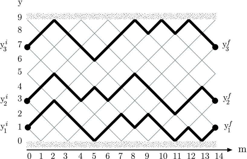
Figure 1: Three non-intersecting directed walks of length $t=14$ in a strip of width $L=9$. The variables $m$, $y_{j}^{i}$ and $y_{j}^{f}$ shown. The walk closest to the lower wall has weight $v(1)w(1,2)w(2,3)w(3,2)\cdots w(1,0)w(0,1)$ with $y^{i}_{1}=1$ and $y^{f}_{1}=1$.

Precisely, we will show that the partition or generating function, ${\stackrel{{\scriptstyle=}}{{Z}}}^{\rm{\cal{N}}}_{t}({\bf y}^{i}\!\rightarrow\!{\bf y}^{f})$, for non-intersecting walk configurations of $N$ walks in which the $j^{th}$ walk starts at $y_{j}^{i}$ and arrives at $y_{j}^{f}$ after $t$ steps is given by the following determinant:

$${\stackrel{{\scriptstyle=}}{{Z}}}^{\rm{\cal{N}}}_{t}({\bf y}^{i}\!\rightarrow\!{\bf y}^{f})=\left|\begin{array}[]{cccc}{\stackrel{{\scriptstyle=}}{{Z}}}^{\rm{\cal{S}}}_{t}(y_{1}^{i}\!\rightarrow\!y_{1}^{f})&{\stackrel{{\scriptstyle=}}{{Z}}}^{\rm{\cal{S}}}_{t}(y_{1}^{i}\!\rightarrow\!y_{2}^{f})&\dots&{\stackrel{{\scriptstyle=}}{{Z}}}^{\rm{\cal{S}}}_{t}(y_{1}^{i}\!\rightarrow\!y_{N}^{f})\\ {\stackrel{{\scriptstyle=}}{{Z}}}^{\rm{\cal{S}}}_{t}(y_{2}^{i}\!\rightarrow\!y_{1}^{f})&{\stackrel{{\scriptstyle=}}{{Z}}}^{\rm{\cal{S}}}_{t}(y_{2}^{i}\!\rightarrow\!y_{2}^{f})&\dots&{\stackrel{{\scriptstyle=}}{{Z}}}^{\rm{\cal{S}}}_{t}(y_{2}^{i}\!\rightarrow\!y_{N}^{f})\\ .&.&.&.\\ .&.&.&.\\ .&.&.&.\\ {\stackrel{{\scriptstyle=}}{{Z}}}^{\rm{\cal{S}}}_{t}(y_{N}^{i}\!\rightarrow\!y_{1}^{f})&{\stackrel{{\scriptstyle=}}{{Z}}}^{\rm{\cal{S}}}_{t}(y_{N}^{i}\!\rightarrow\!y_{2}^{f})&\dots&{\stackrel{{\scriptstyle=}}{{Z}}}^{\rm{\cal{S}}}_{t}(y_{N}^{i}\!\rightarrow\!y_{N}^{f})\end{array}\right|$$ (2.4)

where ${\stackrel{{\scriptstyle=}}{{Z}}}^{\rm{\cal{S}}}_{t}(y_{j}^{i}\!\rightarrow\!y_{k}^{f})$ is the generating function for configurations of a single walk starting at $y_{j}^{i}$ and ending at $y_{k}^{f}$ in a strip of width $L$. This is then a generalisation of the ‘master formulae’ of Fisher (equation (5.9) of [4]) and of Forrester (equation (4) of [5]) where unweighted non-intersecting walks are considered. Importantly, this determinantal result is precisely that given by the very general Gessel-Viennot Theorem [9, 8] for this problem: the walks considered on this lattice with the generalised weights considered satisfy the conditions of the theorem (see [10] for a discussion of a one wall case with homogeneous weights).

3 From Bethe Ansatz to determinant

3.1 Transfer matrix formulation

The generating function of our walk problem in a strip can be formulated as the matrix element of a product of so-called transfer matrices (see below for their precise definition). This ‘transfer matrix’ contains the weights of all the possible edge configurations of $N$ walks of two adjacent columns of sites. As such it is related to an invariant subspace of the full six-vertex transfer matrix [10]. In other words the non-zero elements of the six-vertex transfer matrix occur in diagonal blocks each of which is an “$N$-walk transfer matrix” for some $N$. There are of course several ways of setting up a strip transfer matrix. The most common are the site-to-site and the edge-to-edge matrices which add either edges or sites respectively to the walks. In the case of the six-vertex model the edge-to-edge matrix is usually chosen. Our choice of vertex-to-vertex (we shall use vertex and site interchangeably) matrix is determined by the requirements that the corresponding eigenvalue problem be as simple as possible while ensuring the non-intersecting constraint can be easily implemented.

The calculation of the generating function using the transfer matrix formulation then hinges on the spectral decomposition of the matrix. The matrices we diagonalise will be matrices that add two-steps to the evaluation of the generating function at a time. However the generating function is initially constructed in terms of one-step transfer matrices as these are useful since the non-intersecting condition is explicit.

Definition 1.

Let $y\in\,\stackrel{{\scriptstyle{\scriptscriptstyle\,e}}}{{\cal S}}_{L}$ and $y^{\prime}\in\,\stackrel{{\scriptstyle{\scriptscriptstyle\,o}}}{{\cal S}}_{L}$. For $N=1$ the one-step transfer matrices are defined as

$$\left(\stackrel{{\scriptstyle eo}}{{\mathbf{T}}}_{1}\right)_{y,y^{\prime}} =\begin{cases}0&\text{if $|y-y^{\prime}|>1$}\\ w(y,y^{\prime})&\text{if $|y-y^{\prime}|=1$}\end{cases}$$ (3.5a)

and

$$\left(\stackrel{{\scriptstyle oe}}{{\mathbf{T}}}_{1}\right)_{y^{\prime},y} =\begin{cases}0&\text{if $|y^{\prime}-y|>1$}\\ w(y^{\prime},y)&\text{if $|y-y^{\prime}|=1$}.\end{cases}$$ (3.5b)

The $N$-walk transfer matrices for $N>1$ are constructed from sub-matrices of a direct product of the above $N=1$ matrices:

$$({\stackrel{{\scriptstyle oe}}{{\mathbf{T}}}_{N}})_{{\bf y},{\bf y}^{\prime}} =\left(\bigotimes_{i=1}^{N}\stackrel{{\scriptstyle oe}}{{\mathbf{T}}}_{1}\right)_{{\bf y},{\bf y}^{\prime}}\qquad\qquad\text{${\bf y}\in\,\stackrel{{\scriptstyle{\scriptscriptstyle\,o}}}{{\cal U}}_{L}$ and ${\bf y}^{\prime}\in\,\stackrel{{\scriptstyle{\scriptscriptstyle\,e}}}{{\cal U}}_{L}$}$$ (3.6a)

and

$$({\stackrel{{\scriptstyle eo}}{{\mathbf{T}}}_{N}})_{{\bf y}^{\prime},{\bf y}} =\left(\bigotimes_{i=1}^{N}\stackrel{{\scriptstyle eo}}{{\mathbf{T}}}_{1}\right)_{{\bf y}^{\prime},{\bf y}}\qquad\qquad\text{${\bf y}^{\prime}\in\,\stackrel{{\scriptstyle{\scriptscriptstyle\,e}}}{{\cal U}}_{L}$ and ${\bf y}\in\,\stackrel{{\scriptstyle{\scriptscriptstyle\,o}}}{{\cal U}}_{L}$}$$ (3.6b)

Note that since we are only considering $L$ being odd we have that ${\stackrel{{\scriptstyle oe}}{{\mathbf{T}}}_{N}}$ and ${\stackrel{{\scriptstyle eo}}{{\mathbf{T}}}_{N}}$ are square matrices and that in general $\left(\stackrel{{\scriptstyle oe}}{{\mathbf{T}}}_{1}\right)_{y^{\prime},y}\neq\left(\stackrel{{\scriptstyle eo}}{{\mathbf{T}}}_{1}\right)_{y,y^{\prime}}$. More importantly, the restriction of the row and column spaces of the direct product eliminates the possibility of two walks arriving at the same lattice point. Furthermore the condition that the one-walker transfer matrix vanishes for $|y^{\prime}-y|>1$ prevents the generation of configurations in which pairs of walks “cross” without sharing a common lattice site (only nearest neighbour steps are allowed in all cases). This “non-crossing” condition is unnecessarily restrictive in the one-walk case. However, for $N>1$, if further neighbour steps are allowed then, in general, it is not possible to use the Bethe Ansatz. This condition is the analogue of the “non-crossing condition” of the Gessel-Viennot Theorem.

The generating function ${\stackrel{{\scriptstyle=}}{{Z}}}^{\rm{\cal{N}}}_{t}({\bf y}^{i}\!\rightarrow\!{\bf y}^{f})$ of $N$ non-intersecting walks of length $t$ in a strip is related to ${\stackrel{{\scriptstyle=}}{{Z}}}^{\rm{\cal{N}}}_{t-1}({\bf y}^{i}\!\rightarrow\!\bf{y})$ by recurrence, the coefficients of which are the elements of one of the two one-step transfer matrices defined above. This relationship is given by the following lemma.

Lemma 1.

The generating function ${\stackrel{{\scriptstyle=}}{{Z}}}^{\rm{\cal{N}}}_{t}({\bf y}^{i}\!\rightarrow\!{\bf y}^{f})$ is given for $t>0$, depending on whether ${\bf y}^{f}\in\,\stackrel{{\scriptstyle{\scriptscriptstyle\,e}}}{{\cal U}}_{L}$ or not, by

$${\stackrel{{\scriptstyle=}}{{Z}}}^{\rm{\cal{N}}}_{t}({\bf y}^{i}\!\rightarrow\!{\bf y}^{f})=\left\{\begin{array}[]{l}\sum_{{\bf y}\in\,\stackrel{{\scriptstyle{\scriptscriptstyle\,e}}}{{\cal U}}_{L}}{\stackrel{{\scriptstyle=}}{{Z}}}^{\rm{\cal{N}}}_{t-1}({\bf y}^{i}\!\rightarrow\!{\bf y})({\stackrel{{\scriptstyle eo}}{{\mathbf{T}}}_{N}})_{{\bf y},{\bf y}^{f}}\qquad\hbox{for}\qquad{\bf y}^{f}\in\,\stackrel{{\scriptstyle{\scriptscriptstyle\,o}}}{{\cal U}}_{L}\\ \\ \sum_{{\bf y}\in\,\stackrel{{\scriptstyle{\scriptscriptstyle\,o}}}{{\cal U}}_{L}}{\stackrel{{\scriptstyle=}}{{Z}}}^{\rm{\cal{N}}}_{t-1}({\bf y}^{i}\!\rightarrow\!{\bf y})({\stackrel{{\scriptstyle oe}}{{\mathbf{T}}}_{N}})_{{\bf y},{\bf y}^{f}}\qquad\hbox{for}\qquad{\bf y}^{f}\in\,\stackrel{{\scriptstyle{\scriptscriptstyle\,e}}}{{\cal U}}_{L}\;.\end{array}\right.$$ (3.7)

Proof.

A simple proof of this Lemma can be constructed using induction on $t$. ∎

Together with the initial condition

$${\stackrel{{\scriptstyle=}}{{Z}}}^{\rm{\cal{N}}}_{0}({\bf y}^{i}\!\rightarrow\!{\bf y}^{f})=\delta_{{\bf y}^{i},{\bf y}^{f}}V({\bf y}^{i}),$$ (3.8)

where

$$V({\bf y}^{i})=\prod_{\alpha=1}^{N}v(y^{i}_{\alpha}),$$ (3.9)

equation (3.7) determines ${\stackrel{{\scriptstyle=}}{{Z}}}^{\rm{\cal{N}}}_{t}({\bf y}^{i}\!\rightarrow\!{\bf y}^{f})$.

A simple corollary of this Lemma (again shown by induction) is that the partition function can be written in terms of “two-step” transfer matrices.

Corollary.

The generating function ${\stackrel{{\scriptstyle=}}{{Z}}}^{\rm{\cal{N}}}_{t}({\bf y}^{i}\!\rightarrow\!{\bf y}^{f})$ is given, depending on whether $t$ is even or odd, as

$${\stackrel{{\scriptstyle=}}{{Z}}}^{\rm{\cal{N}}}_{2r}({\bf y}^{i}\!\rightarrow\!{\bf y}^{f}) =\left\{\begin{array}[]{ll}V({\bf y}^{i})\left((\stackrel{{\scriptstyle e\cdot e}}{{\mathbf{T}}}_{N})^{r}\right)_{{\bf y}^{i},{\bf y}^{f}}&\hbox{for}\quad{\bf y}^{i}\in\,\stackrel{{\scriptstyle{\scriptscriptstyle\,e}}}{{\cal U}}_{L}\hbox{ and }{\bf y}^{f}\in\,\stackrel{{\scriptstyle{\scriptscriptstyle\,e}}}{{\cal U}}_{L}\\ \\ V({\bf y}^{i})\left((\stackrel{{\scriptstyle o\cdot o}}{{\mathbf{T}}}_{N})^{r}\right)_{{\bf y}^{i},{\bf y}^{f}}&\hbox{for}\quad{\bf y}^{i}\in\,\stackrel{{\scriptstyle{\scriptscriptstyle\,o}}}{{\cal U}}_{L}\hbox{ and }{\bf y}^{f}\in\,\stackrel{{\scriptstyle{\scriptscriptstyle\,o}}}{{\cal U}}_{L}\end{array}\right.$$ (3.10d)

or

$${\stackrel{{\scriptstyle=}}{{Z}}}^{\rm{\cal{N}}}_{2r+1}({\bf y}^{i}\!\rightarrow\!{\bf y}^{f}) =\left\{\begin{array}[]{ll}V({\bf y}^{i})\sum_{{\bf y}\in\,\stackrel{{\scriptstyle{\scriptscriptstyle\,e}}}{{\cal U}}_{L}}\left((\stackrel{{\scriptstyle e\cdot e}}{{\mathbf{T}}}_{N})^{r}\right)_{{\bf y}^{i},{\bf y}}({\stackrel{{\scriptstyle eo}}{{\mathbf{T}}}_{N}})_{{\bf y},{\bf y}^{f}}&\hbox{for}\quad{\bf y}^{i}\in\,\stackrel{{\scriptstyle{\scriptscriptstyle\,e}}}{{\cal U}}_{L}\hbox{ and }{\bf y}^{f}\in\,\stackrel{{\scriptstyle{\scriptscriptstyle\,o}}}{{\cal U}}_{L}\\ \\ V({\bf y}^{i})\sum_{{\bf y}\in\,\stackrel{{\scriptstyle{\scriptscriptstyle\,o}}}{{\cal U}}_{L}}\left((\stackrel{{\scriptstyle o\cdot o}}{{\mathbf{T}}}_{N})^{r}\right)_{{\bf y}^{i},{\bf y}}({\stackrel{{\scriptstyle oe}}{{\mathbf{T}}}_{N}})_{{\bf y},{\bf y}^{f}}&\hbox{for}\quad{\bf y}^{i}\in\,\stackrel{{\scriptstyle{\scriptscriptstyle\,o}}}{{\cal U}}_{L}\hbox{ and }{\bf y}^{f}\in\,\stackrel{{\scriptstyle{\scriptscriptstyle\,e}}}{{\cal U}}_{L}\end{array}\right.$$ (3.10h)

for $r=0,1,2,\dots$, where the two-step transfer matrices are defined as

$$\stackrel{{\scriptstyle e\cdot e}}{{\mathbf{T}}}_{N} ={\stackrel{{\scriptstyle eo}}{{\mathbf{T}}}_{N}}\,{\stackrel{{\scriptstyle oe}}{{\mathbf{T}}}_{N}}$$ (3.11a)

$$\stackrel{{\scriptstyle o\cdot o}}{{\mathbf{T}}}_{N} ={\stackrel{{\scriptstyle oe}}{{\mathbf{T}}}_{N}}\,{\stackrel{{\scriptstyle eo}}{{\mathbf{T}}}_{N}}.$$ (3.11b)

The two-step transfer matrices correspond to adding two steps to the paths. We show below that the generating function ${\stackrel{{\scriptstyle=}}{{Z}}}^{\rm{\cal{N}}}_{t}({\bf y}^{i}\!\rightarrow\!{\bf y}^{f})$ may in fact be expressed in terms of the eigenvalues and eigenvectors of the two-step matrices. In general the two-step matrices are not symmetric and hence one has to consider left and right eigenvectors. The $N$-walk eigenvectors will be constructed from the one-walk eigenvectors via the Bethe Ansatz. Used in this context the Ansatz expresses the components of the $N$-walk eigenvectors as a determinant of the components of one-walk eigenvectors (see (3.17) below).

3.2 From transfer matrices to determinants

This section contains our main results in the form of two theorems that state under what conditions the $N$-walk generating function can be written as the determinant (2.4). In summary, our theorems proven below show that the equivalence of the Bethe Ansatz in the form of equation (3.17) and the result of the Gessel-Viennot Theorem in the form (3.33) rests on showing that for any given problem the Ansatz is sufficiently good to provide a spanning (or complete) set of eigenvectors. This in turn depends only on the completeness of the one-walk eigenvectors (conditions of Lemma 2).

In this paper it is not our purpose to prove that all choices of the functions $w(y,y^{\prime})$ which make up the elements of the one-walk transfer matrices allow for the conditions of our theorems to be satisfied. However, these theorems have been subsequently used to analyse some interesting cases in detail [3] where as a consequence we show that an arbitrary boundary weight on one boundary (and special weight on the other) with homogeneous weights otherwise satisfies the conditions of the theorems. Also, we point out that since the Gessel-Viennot determinant holds for any function $w(y,y^{\prime})$ it is almost certainly true that our conditions are satisfied always. It is however our main purpose here to demonstrate how the Bethe Ansatz gives the solution of the $N$-walk problem given the solution of the one-walk problem.

The first theorem states the conditions under which the $N$-walk transfer matrices can be diagonalised using a Bethe Ansatz: the major condition is that the one-walk transfer matrix problem can be solved — see Lemma 2. The second theorem basically states that if the Bethe Ansatz gives a complete set of eigenvectors for the $N$-walk problem for any $N$, then the $N$-walk generating function is a determinant of one-walk generating functions.

To begin we set up the conditions that define a solution of the one-walk problem: these will be the conditions our two theorems require.

Lemma 2.

Suppose that there exist linearly independent sets of column vectors $\{\stackrel{{\scriptstyle o}}{{\varphi}}{\!\!}^{\mbox{\tiny R}}_{{k}}\}_{k\in{\cal K}_{1}}$ and $\{\stackrel{{\scriptstyle e}}{{\varphi}}{\!\!}^{\mbox{\tiny R}}_{{k}}\}_{k\in{\cal K}_{1}}$, where ${\cal K}_{1}$ is some index set, which satisfy

$$\stackrel{{\scriptstyle eo}}{{\mathbf{T}}}_{1}\stackrel{{\scriptstyle o}}{{\varphi}}{\!\!}^{\mbox{\tiny R}}_{{k}}=\lambda_{k}\stackrel{{\scriptstyle e}}{{\varphi}}{\!\!}^{\mbox{\tiny R}}_{{k}}\qquad\hbox{and}\qquad\stackrel{{\scriptstyle oe}}{{\mathbf{T}}}_{1}\stackrel{{\scriptstyle e}}{{\varphi}}{\!\!}^{\mbox{\tiny R}}_{{k}}=\lambda_{k}\stackrel{{\scriptstyle o}}{{\varphi}}{\!\!}^{\mbox{\tiny R}}_{{k}}$$ (3.12)

with $\lambda_{k}\in\mathbb{C}$, and which span the column spaces of $\stackrel{{\scriptstyle eo}}{{\mathbf{T}}}_{1}$ and $\stackrel{{\scriptstyle oe}}{{\mathbf{T}}}_{1}$ respectively (in which case they are said to be complete). Further let $\stackrel{{\scriptstyle e\cdot e}}{{\mathbf{T}}}_{1}$ and $\stackrel{{\scriptstyle o\cdot o}}{{\mathbf{T}}}_{1}$ be defined by (3.11) then

• $\stackrel{{\scriptstyle o}}{{\varphi}}{\!\!}^{\mbox{\tiny R}}_{{k}}$ and $\stackrel{{\scriptstyle e}}{{\varphi}}{\!\!}^{\mbox{\tiny R}}_{{k}}$ are right eigenvectors of $\stackrel{{\scriptstyle o\cdot o}}{{\mathbf{T}}}_{1}$ and $\stackrel{{\scriptstyle e\cdot e}}{{\mathbf{T}}}_{1}$ respectively with eigenvalue $\lambda_{k}^{2}$.

• corresponding sets $\{\stackrel{{\scriptstyle o}}{{\varphi}}{\!\!}^{\mbox{\tiny L}}_{{k}}\}_{k\in{\cal K}_{1}}$ and $\{\stackrel{{\scriptstyle e}}{{\varphi}}{\!\!}^{\mbox{\tiny L}}_{{k}}\}_{k\in{\cal K}_{1}}$ of row vectors may be found such that

  $$\stackrel{{\scriptstyle p}}{{\varphi}}{\!\!}^{\mbox{\tiny L}*}_{{k}}\cdot\stackrel{{\scriptstyle p}}{{\varphi}}{\!\!}^{\mbox{\tiny R}}_{{k^{\prime}}}=\delta_{k,k^{\prime}}\qquad\hbox{and}\qquad\sum_{k\in{\cal K}_{1}}\stackrel{{\scriptstyle p}}{{\varphi}}{\!\!}^{\mbox{\tiny R}}_{{k}}(y)\stackrel{{\scriptstyle p}}{{\varphi}}{\!\!}^{\mbox{\tiny L}*}_{{k}}(y^{\prime})=\delta_{y,y^{\prime}}$$ (3.13)

  for each $p\in\{e,o\}$, where the $*$ denotes complex conjugation. Note that the vectors of (3.13) have components indexed by $y$.

• the row vectors of (ii) satisfy

  $$\stackrel{{\scriptstyle o}}{{\varphi}}{\!\!}^{\mbox{\tiny L}}_{{k}}\stackrel{{\scriptstyle oe}}{{\mathbf{T}}}_{1}=\lambda_{k}\stackrel{{\scriptstyle e}}{{\varphi}}{\!\!}^{\mbox{\tiny L}}_{{k}}\qquad\hbox{and}\qquad\stackrel{{\scriptstyle e}}{{\varphi}}{\!\!}^{\mbox{\tiny L}}_{{k}}\stackrel{{\scriptstyle eo}}{{\mathbf{T}}}_{1}=\lambda_{k}\stackrel{{\scriptstyle o}}{{\varphi}}{\!\!}^{\mbox{\tiny L}}_{{k}}$$ (3.14)

  and also $\stackrel{{\scriptstyle o}}{{\varphi}}{\!\!}^{\mbox{\tiny L}}_{{k}}$ and $\stackrel{{\scriptstyle e}}{{\varphi}}{\!\!}^{\mbox{\tiny L}}_{{k}}$ are left eigenvectors of $\stackrel{{\scriptstyle o\cdot o}}{{\mathbf{T}}}_{1}$ and $\stackrel{{\scriptstyle e\cdot e}}{{\mathbf{T}}}_{1}$ respectively with eigenvalue $\lambda_{k}^{2}$.

Note that since the vectors in (3.12) span the space the cardinality of the index set ${\cal K}_{1}$ is $(L+1)/2$. The proof of the lemma is elementary linear algebra and we omit it. Notice that if $\lambda_{k}$ is a solution of (3.12) then so is $-\lambda_{k}$ with vector $\stackrel{{\scriptstyle e}}{{\varphi}}{\!\!}^{\mbox{\tiny R}}_{{k}}$ replaced by $-\stackrel{{\scriptstyle e}}{{\varphi}}{\!\!}^{\mbox{\tiny R}}_{{k}}$. These vectors are clearly not independent and normally sufficient independent vectors to form a spanning set are obtained by taking only the positive values of $\lambda_{k}$.

From the above left and right one-walk vectors we now construct the $N$-walk vectors and hence eigenvectors of $\stackrel{{\scriptstyle e\cdot e}}{{\mathbf{T}}}_{N}$ and $\stackrel{{\scriptstyle o\cdot o}}{{\mathbf{T}}}_{N}$.

Theorem 1.

Let $\stackrel{{\scriptstyle e\cdot e}}{{\mathbf{T}}}_{N}$ and $\stackrel{{\scriptstyle o\cdot o}}{{\mathbf{T}}}_{N}$, $N>1$, be given by equations (3.11). By imposing an arbitrary ordering on the elements of ${\cal K}_{1}$ define

$${\cal K}_{N}=\{{\bf k}=(k_{1},k_{2},\dots k_{N})|k_{i}\in{\cal K}_{1}\mbox{ and }k_{1}<k_{2}<\dots<k_{N}\}$$ (3.15)

and

$$\Lambda_{{\bf k}}=\prod_{\alpha=1}^{N}\lambda_{k_{\alpha}}.$$ (3.16)

(a) If for $C\in\{L,R\}$ and $p\in\{e,o\}$, $\{\stackrel{{\scriptstyle p}}{{\varphi}}{\!\!}^{\mbox{\tiny C}}_{{k}}\}_{k\in{\cal K}_{1}}$ satisfy the conditions of Lemma 2 then the vectors $\{\stackrel{{\scriptstyle p}}{{\Phi}}{\!\!}^{\mbox{\tiny C}}_{{{\bf k}}}\}_{{\bf k}\in{\cal K}_{N}}$ given by the Bethe Ansatz,

$$\stackrel{{\scriptstyle p}}{{\Phi}}{\!\!}^{\mbox{\tiny C}}_{{{\bf k}}}({\bf y})= \sum_{\sigma\in P_{N}}\epsilon_{\sigma}\prod_{\alpha=1}^{N}\stackrel{{\scriptstyle p}}{{\varphi}}{\!\!}^{\mbox{\tiny C}}_{{k_{\sigma_{\alpha}}}}(y_{\alpha})=\sum_{\sigma\in P_{N}}\epsilon_{\sigma}\prod_{\alpha=1}^{N}\stackrel{{\scriptstyle p}}{{\varphi}}{\!\!}^{\mbox{\tiny C}}_{{k_{{\alpha}}}}(y_{\sigma_{\alpha}})\qquad\text{${\bf y}\in\,\stackrel{{\scriptstyle{\scriptscriptstyle\,p}}}{{\cal U}}_{L}$},$$ (3.17)

where $P_{N}$ is the set of $N!$ permutations of $\{1,2,\ldots,N\}$, $\sigma=(\sigma_{1},\sigma_{2},\ldots,\sigma_{N})\in P_{N}$ and $\epsilon_{\sigma}$ is the signature of the permutation $\sigma$, satisfy

$${\stackrel{{\scriptstyle oe}}{{\mathbf{T}}}_{N}}\stackrel{{\scriptstyle e}}{{\Phi}}{\!\!}^{\mbox{\tiny R}}_{{{\bf k}}}=\Lambda_{{\bf k}}\stackrel{{\scriptstyle o}}{{\Phi}}{\!\!}^{\mbox{\tiny R}}_{{{\bf k}}}\qquad\hbox{and}\qquad{\stackrel{{\scriptstyle eo}}{{\mathbf{T}}}_{N}}\stackrel{{\scriptstyle o}}{{\Phi}}{\!\!}^{\mbox{\tiny R}}_{{{\bf k}}}=\Lambda_{{\bf k}}\stackrel{{\scriptstyle e}}{{\Phi}}{\!\!}^{\mbox{\tiny R}}_{{{\bf k}}}.$$ (3.18)

(b) Moreover the conclusions of parts (i), (ii) and (iii) of Lemma 2 hold with $\stackrel{{\scriptstyle p}}{{\varphi}}{\!\!}^{\mbox{\tiny C}}_{{k}}$ replaced by $\stackrel{{\scriptstyle p}}{{\Phi}}{\!\!}^{\mbox{\tiny C}}_{{{\bf k}}}$, $\stackrel{{\scriptstyle eo}}{{\mathbf{T}}}_{1}$ and $\stackrel{{\scriptstyle oe}}{{\mathbf{T}}}_{1}$ replaced by ${\stackrel{{\scriptstyle eo}}{{\mathbf{T}}}_{N}}$ and ${\stackrel{{\scriptstyle oe}}{{\mathbf{T}}}_{N}}$, ${\cal K}_{1}$ replaced by ${\cal K}_{N}$, and $\lambda_{k}$ replaced by $\Lambda_{{\bf k}}$.

The proofs of part of this theorem and Theorem 2 require the following result.

Proposition 1.

For ${\bf k}\in\,{\cal K}_{N}$ and ${\bf y}\in\,\,\stackrel{{\scriptstyle{\scriptscriptstyle\,p}}}{{\cal U}}_{L}$ let

$$\Phi_{\bf k}({\bf y})=\sum_{\sigma\in P_{N}}\epsilon_{\sigma}\prod_{\alpha=1}^{N}\phi_{k_{{\sigma_{\alpha}}}}(y_{\alpha})\qquad\hbox{and}\qquad\Psi_{\bf k}({\bf y})=\sum_{\sigma\in P_{N}}\epsilon_{\sigma}\prod_{\alpha=1}^{N}\psi_{k_{\sigma_{\alpha}}}(y_{\alpha}).$$ (3.19)

Also let

$$f({\bf k})=\prod_{\alpha=1}^{N}f(k_{\alpha})$$ (3.20)

then

$$\sum_{{\bf k}\,\in\,{\cal K}_{N}}f({\bf k})\Phi_{\bf k}({\bf y})\Psi_{\bf k}({\bf y}^{\prime})=\sum_{\sigma\in P_{N}}\epsilon_{\sigma}\prod_{\alpha=1}^{N}\left(\sum_{k_{\alpha}\in\,{\cal K}_{1}}f(k_{\alpha})\phi_{k_{{\alpha}}}(y_{\alpha})\psi_{k_{\alpha}}(y_{\sigma_{\alpha}}^{\prime})\right)$$ (3.21)

and

$$\sum_{{\bf y}\,\in\,\,\stackrel{{\scriptstyle{\scriptscriptstyle\,p}}}{{\cal U}}_{L}}\Phi_{\bf k}({\bf y})\Psi_{{\bf k}^{\prime}}({\bf y})=\sum_{\sigma\in P_{N}}\epsilon_{\sigma}\prod_{\alpha=1}^{N}\left(\sum_{y_{\alpha}\,\in\,\stackrel{{\scriptstyle{\scriptscriptstyle\,p}}}{{\cal S}}_{L}}\phi_{k_{{\alpha}}}(y_{\alpha})\psi_{k_{\sigma_{\alpha}}^{\prime}}(y_{\alpha})\right)$$ (3.22)

Proof.

$$\sum_{{\bf k}\,\in\,{\cal K}_{N}}f({\bf k})\Phi_{\bf k}({\bf y})\Psi_{\bf k}({\bf y}^{\prime})= \sum_{\sigma\in P_{N}}\epsilon_{\sigma}\sum_{{\bf k}\,\in\,{\cal K}_{N}}\sum_{\tau\in P_{N}}\epsilon_{\tau}\prod_{\alpha=1}^{N}f(k_{\alpha})\phi_{k_{{\tau_{\alpha}}}}(y_{\alpha})\psi_{k_{{\sigma_{\alpha}}}}(y_{\alpha}^{\prime})$$ (3.23)

$$= \sum_{\sigma^{\prime}\in P_{N}}\epsilon_{\sigma^{\prime}}\sum_{{\bf k}\,\in\,{\cal K}_{N}}\sum_{\tau\in P_{N}}\prod_{\alpha=1}^{N}f(k_{\alpha})\phi_{k_{{\tau_{\alpha}}}}(y_{\alpha})\psi_{k_{{\tau_{\alpha}}}}(y_{\sigma^{\prime}_{\alpha}}^{\prime})$$ (3.24)

The double sum over permutations, $\tau$ and ${\bf k}\in{\cal K}_{N}$ is equivalent to summing each $k_{\alpha}$ independently over ${\cal K}_{1}$ (terms for which two or more components of ${\bf k}$ are equal make zero contribution) and the first result follows. The second result follows in the same way by interchanging the roles of $k$ and $y$. ∎

Proof.

(of Theorem 1 ) (a) We first obtain the cyclic property (3.18) as follows.

$$\left({\stackrel{{\scriptstyle oe}}{{\mathbf{T}}}_{N}}\stackrel{{\scriptstyle e}}{{\Phi}}{\!\!}^{\mbox{\tiny R}}_{{{\bf k}}}\right)_{\bf y} =\sum_{{\bf y}^{\prime}\in\,\stackrel{{\scriptstyle{\scriptscriptstyle\,e}}}{{\cal U}}_{L}}\sum_{\sigma\in P_{N}}\epsilon_{\sigma}\left({\stackrel{{\scriptstyle oe}}{{\mathbf{T}}}_{N}}\right)_{{\bf y},{\bf y}^{\prime}}\prod_{\alpha=1}^{N}\stackrel{{\scriptstyle e}}{{\varphi}}{\!\!}^{\mbox{\tiny R}}_{{k_{\sigma_{\alpha}}}}(y^{\prime}_{\alpha})$$ (3.25a)

$$=\sum_{\sigma\in P_{N}}\epsilon_{\sigma}\sum_{{\bf y}^{\prime}\in\,\stackrel{{\scriptstyle{\scriptscriptstyle\,e}}}{{\cal U}}_{L}}\prod_{\alpha=1}^{N}\left(\stackrel{{\scriptstyle oe}}{{\mathbf{T}}}_{1}\right)_{y_{\alpha},y^{\prime}_{\alpha}}\stackrel{{\scriptstyle e}}{{\varphi}}{\!\!}^{\mbox{\tiny R}}_{{k_{\sigma_{\alpha}}}}(y^{\prime}_{\alpha})\qquad\left(\hbox{using}\quad\eqref{eq:t-N}\right)$$ (3.25b)

$$=\sum_{\sigma\in P_{N}}\epsilon_{\sigma}\left[\sum_{y^{\prime}_{1}\in\,\stackrel{{\scriptstyle{\scriptscriptstyle\,e}}}{{\cal S}}_{L}}\left(\stackrel{{\scriptstyle oe}}{{\mathbf{T}}}_{1}\right)_{y_{1},y^{\prime}_{1}}\stackrel{{\scriptstyle e}}{{\varphi}}{\!\!}^{\mbox{\tiny R}}_{{k_{\sigma_{1}}}}(y^{\prime}_{1})\right]\ldots\left[\sum_{y^{\prime}_{N}\in\,\stackrel{{\scriptstyle{\scriptscriptstyle\,e}}}{{\cal S}}_{L}}\left(\stackrel{{\scriptstyle oe}}{{\mathbf{T}}}_{1}\right)_{y_{N},y^{\prime}_{N}}\stackrel{{\scriptstyle e}}{{\varphi}}{\!\!}^{\mbox{\tiny R}}_{{k_{\sigma_{N}}}}(y^{\prime}_{N})\right]$$ (3.25c)

$$=\sum_{\sigma\in P_{N}}\epsilon_{\sigma}\,\left[\lambda_{k_{\sigma_{1}}}\stackrel{{\scriptstyle o}}{{\varphi}}{\!\!}^{\mbox{\tiny R}}_{{k_{\sigma_{1}}}}(y_{1})\right]\ldots\left[\lambda_{k_{\sigma_{N}}}\stackrel{{\scriptstyle o}}{{\varphi}}{\!\!}^{\mbox{\tiny R}}_{{k_{\sigma_{N}}}}(y_{N})\right]\qquad\left(\hbox{using}\quad\eqref{eq:cyclic-rR}\right)$$ (3.25d)

$$=\Lambda_{{\bf k}}\,\stackrel{{\scriptstyle o}}{{\Phi}}{\!\!}^{\mbox{\tiny R}}_{{{\bf k}}}({\bf y})$$ (3.25e)

The critical step, and the whole reason for introducing the Bethe Ansatz, is to enable one to go from the restricted sums of (3.25b) to the unrestricted sums in (3.25c). This is justified for two reasons,

1. since $\stackrel{{\scriptstyle e}}{{\Phi}}{\!\!}^{\mbox{\tiny R}}_{{{\bf k}}}({\bf y}^{\prime})$ is a determinant, if any of the $y_{\alpha}$’s are equal then $\stackrel{{\scriptstyle e}}{{\Phi}}{\!\!}^{\mbox{\tiny R}}_{{{\bf k}}}=0$ – this allows the restriction $y^{\prime}_{1}<y^{\prime}_{2}\ldots<y^{\prime}_{N}$ on the sum to be relaxed to $y^{\prime}_{1}\leq y^{\prime}_{2}\ldots\leq y^{\prime}_{N}$

2. the $y_{\alpha}$ are in strictly increasing order combined with the fact that the matrix elements of $\stackrel{{\scriptstyle oe}}{{\mathbf{T}}}_{1}$, are only non-zero if $|y_{\alpha}-y^{\prime}_{\alpha}|\leq 1$ allows the restriction on the sum to be removed altogether.

The second part of (3.18) follows mutatis mutandis.

(b) (i) The vector $\stackrel{{\scriptstyle e}}{{\Phi}}{\!\!}^{\mbox{\tiny R}}_{{{\bf k}}}$ is a right eigenvector of $\stackrel{{\scriptstyle e\cdot e}}{{\mathbf{T}}}_{N}$ with eigenvalue $\Lambda_{{\bf k}}^{2}$, since

$$\stackrel{{\scriptstyle e\cdot e}}{{\mathbf{T}}}_{N}\stackrel{{\scriptstyle e}}{{\Phi}}{\!\!}^{\mbox{\tiny R}}_{{{\bf k}}}={\stackrel{{\scriptstyle eo}}{{\mathbf{T}}}_{N}}{\stackrel{{\scriptstyle oe}}{{\mathbf{T}}}_{N}}\stackrel{{\scriptstyle e}}{{\Phi}}{\!\!}^{\mbox{\tiny R}}_{{{\bf k}}}={\stackrel{{\scriptstyle eo}}{{\mathbf{T}}}_{N}}\Lambda_{{\bf k}}\stackrel{{\scriptstyle o}}{{\Phi}}{\!\!}^{\mbox{\tiny R}}_{{{\bf k}}}=\Lambda_{{\bf k}}^{2}\stackrel{{\scriptstyle e}}{{\Phi}}{\!\!}^{\mbox{\tiny R}}_{{{\bf k}}}$$

which follows from (3.18). Similarly $\stackrel{{\scriptstyle o}}{{\Phi}}{\!\!}^{\mbox{\tiny R}}_{{{\bf k}}}$ is a right eigenvector of $\stackrel{{\scriptstyle o\cdot o}}{{\mathbf{T}}}_{N}$ with eigenvalue $\Lambda_{{\bf k}}^{2}$.

(ii) Let us start by deriving the first result of part (ii), namely the orthogonality and normalisation condition. Using (3.22), for ${\bf k},{\bf k}^{\prime}\in{\cal K}_{N}$

$$\sum_{{\bf y}\in\,\stackrel{{\scriptstyle{\scriptscriptstyle\,p}}}{{\cal U}}_{L}}\stackrel{{\scriptstyle p}}{{\Phi}}{\!\!}^{\mbox{\tiny L}*}_{{{\bf k}}}({\bf y})\stackrel{{\scriptstyle p}}{{\Phi}}{\!\!}^{\mbox{\tiny R}}_{{{\bf k}^{\prime}}}({\bf y})= \sum_{\sigma\in P_{N}}\epsilon_{\sigma}\prod_{\alpha=1}^{N}\left(\sum_{y_{\alpha}\,\in\,\stackrel{{\scriptstyle{\scriptscriptstyle\,p}}}{{\cal S}}_{L}}\stackrel{{\scriptstyle p}}{{\varphi}}{\!\!}^{\mbox{\tiny L}*}_{{k_{\alpha}}}(y_{\alpha})\stackrel{{\scriptstyle p}}{{\varphi}}{\!\!}^{\mbox{\tiny R}}_{{k_{\sigma_{\alpha}}^{\prime}}}(y_{\alpha})\right)$$

$$= \sum_{\sigma\in P_{N}}\epsilon_{\sigma}\prod_{\alpha=1}^{N}\delta_{k_{\alpha},k_{\sigma_{\alpha}}^{\prime}}\qquad\left(\hbox{using}\quad\eqref{oc}\right)$$

$$= \prod_{\alpha=1}^{N}\delta_{k_{\alpha},k_{\alpha}^{\prime}}$$

since the components of ${\bf k}$ and ${\bf k}^{\prime}$ are in the same order only the identity permutation gives a non-zero delta function product. Thus

$$\stackrel{{\scriptstyle p}}{{\Phi}}{\!\!}^{\mbox{\tiny L}*}_{{{\bf k}}}\cdot\stackrel{{\scriptstyle p}}{{\Phi}}{\!\!}^{\mbox{\tiny R}}_{{{\bf k}}}=\delta_{{\bf k},{\bf k}^{\prime}}.$$ (3.26)

Our derivation of the second part of (ii), namely the “completeness condition”, closely parallels the derivation of the orthogonality and normalisation condition. Using (3.21), for ${\bf y},{\bf y}^{\prime}\in\,\stackrel{{\scriptstyle{\scriptscriptstyle\,p}}}{{\cal U}}_{L}$

$$\sum_{{\bf k}\in{\cal K}_{N}}\stackrel{{\scriptstyle p}}{{\Phi}}{\!\!}^{\mbox{\tiny R}}_{{{\bf k}}}({\bf y})\stackrel{{\scriptstyle p}}{{\Phi}}{\!\!}^{\mbox{\tiny L}*}_{{{\bf k}}}({\bf y}^{\prime})= \sum_{\sigma\in P_{N}}\epsilon_{\sigma}\prod_{\alpha=1}^{N}\left(\sum_{k_{\alpha}\,\in{\cal K}_{1}}\stackrel{{\scriptstyle p}}{{\varphi}}{\!\!}^{\mbox{\tiny R}}_{{k_{\alpha}}}(y_{\alpha})\stackrel{{\scriptstyle p}}{{\varphi}}{\!\!}^{\mbox{\tiny L}*}_{{k_{\alpha}}}(y_{\sigma_{\alpha}}^{\prime})\right)$$

$$= \sum_{\sigma\in P_{N}}\epsilon_{\sigma}\prod_{\alpha=1}^{N}\delta_{y_{\alpha},y_{\sigma_{\alpha}}^{\prime}}\qquad\left(\hbox{using}\quad\eqref{oc}\right)$$

$$= \prod_{\alpha=1}^{N}\delta_{y_{\alpha},y_{\alpha}^{\prime}}$$

so

$$\sum_{{\bf k}\in{\cal K}_{N}}\stackrel{{\scriptstyle p}}{{\Phi}}{\!\!}^{\mbox{\tiny R}}_{{{\bf k}}}({\bf y})\stackrel{{\scriptstyle p}}{{\Phi}}{\!\!}^{\mbox{\tiny L}*}_{{{\bf k}}}({\bf y}^{\prime})=\delta_{{\bf y},{\bf y}^{\prime}}$$ (3.27)

Notice that $|{\cal K}_{N}|={{\frac{1}{2}(L+1)}\choose N}$ which is the row (and column) space dimension, as it should be for completeness.

(iii) Using basic linear algebra gives

$$\stackrel{{\scriptstyle o}}{{\Phi}}{\!\!}^{\mbox{\tiny L}}_{{{\bf k}}}{\stackrel{{\scriptstyle oe}}{{\mathbf{T}}}_{N}}=\stackrel{{\scriptstyle e}}{{\Phi}}{\!\!}^{\mbox{\tiny L}}_{{{\bf k}}}\Lambda_{{\bf k}}\qquad\qquad\qquad\stackrel{{\scriptstyle e}}{{\Phi}}{\!\!}^{\mbox{\tiny L}}_{{{\bf k}}}{\stackrel{{\scriptstyle eo}}{{\mathbf{T}}}_{N}}=\stackrel{{\scriptstyle o}}{{\Phi}}{\!\!}^{\mbox{\tiny L}}_{{{\bf k}}}\Lambda_{{\bf k}}$$ (3.28)

and

$$\stackrel{{\scriptstyle e}}{{\Phi}}{\!\!}^{\mbox{\tiny L}}_{{{\bf k}}}\stackrel{{\scriptstyle e\cdot e}}{{\mathbf{T}}}_{N}=\stackrel{{\scriptstyle e}}{{\Phi}}{\!\!}^{\mbox{\tiny L}}_{{{\bf k}}}\Lambda_{{\bf k}}^{2}\qquad\qquad\qquad\stackrel{{\scriptstyle o}}{{\Phi}}{\!\!}^{\mbox{\tiny L}}_{{{\bf k}}}\stackrel{{\scriptstyle o\cdot o}}{{\mathbf{T}}}_{N}=\stackrel{{\scriptstyle o}}{{\Phi}}{\!\!}^{\mbox{\tiny L}}_{{{\bf k}}}\Lambda_{{\bf k}}^{2}$$ (3.29)

∎

Lemma 3.

If the conditions of Theorem 1 hold then

$${\stackrel{{\scriptstyle=}}{{Z}}}^{\rm{\cal{N}}}_{t}({\bf y}^{i}\!\rightarrow\!{\bf y}^{f})=V({\bf y}^{i})\sum_{{\bf k}\in{\cal K}_{N}}\,\,\stackrel{{\scriptstyle p^{\prime}}}{{\Phi}}{\!\!}^{\mbox{\tiny R}}_{{{\bf k}}}({\bf y}^{i})\Lambda^{t}_{{\bf k}}\stackrel{{\scriptstyle p}}{{\Phi}}{\!\!}^{\mbox{\tiny L}*}_{{{\bf k}}}({\bf y}^{f})\qquad{\bf y}^{i}\in\,\stackrel{{\scriptstyle{\scriptscriptstyle\,p^{\prime}}}}{{\cal U}}_{L}\text{and}\quad{\bf y}^{f}\in\,\stackrel{{\scriptstyle{\scriptscriptstyle\,p}}}{{\cal U}}_{L}$$ (3.30)

where if $t$ is even, $p^{\prime}=p$ but otherwise $p$ and $p^{\prime}$ are of opposite parity.

Proof.

If the conditions of Theorem 1 hold then we have that (3.26), (3.27), (3.28) and (3.29) are valid. Using (3.28) and (3.27) it follows that

$$(\,{\stackrel{{\scriptstyle oe}}{{\mathbf{T}}}_{N}})_{{\bf y},{\bf y}^{\prime}}=\sum_{{\bf k}\in{\cal K}_{N}}\Lambda_{{\bf k}}\stackrel{{\scriptstyle o}}{{\Phi}}{\!\!}^{\mbox{\tiny R}}_{{{\bf k}}}({\bf y})\stackrel{{\scriptstyle e}}{{\Phi}}{\!\!}^{\mbox{\tiny L}*}_{{{\bf k}}}({\bf y}^{\prime})\qquad\hbox{and}\qquad(\,{\stackrel{{\scriptstyle eo}}{{\mathbf{T}}}_{N}})_{{\bf y},{\bf y}^{\prime}}=\sum_{{\bf k}\in{\cal K}_{N}}\Lambda_{{\bf k}}\stackrel{{\scriptstyle e}}{{\Phi}}{\!\!}^{\mbox{\tiny R}}_{{{\bf k}}}({\bf y})\stackrel{{\scriptstyle o}}{{\Phi}}{\!\!}^{\mbox{\tiny L}*}_{{{\bf k}}}({\bf y}^{\prime}).$$ (3.31)

Also, using (3.29) and (3.27) it follows that

$$(\,\stackrel{{\scriptstyle e\cdot e}}{{\mathbf{T}}}_{N})_{{\bf y},{\bf y}^{\prime}}=\sum_{{\bf k}\in{\cal K}_{N}}\Lambda_{{\bf k}}^{2}\stackrel{{\scriptstyle e}}{{\Phi}}{\!\!}^{\mbox{\tiny R}}_{{{\bf k}}}({\bf y})\stackrel{{\scriptstyle e}}{{\Phi}}{\!\!}^{\mbox{\tiny L}*}_{{{\bf k}}}({\bf y}^{\prime})\qquad\hbox{and}\qquad(\,\stackrel{{\scriptstyle o\cdot o}}{{\mathbf{T}}}_{N})_{{\bf y},{\bf y}^{\prime}}=\sum_{{\bf k}\in{\cal K}_{N}}\Lambda_{\bf k}^{2}\stackrel{{\scriptstyle o}}{{\Phi}}{\!\!}^{\mbox{\tiny R}}_{{{\bf k}}}({\bf y})\stackrel{{\scriptstyle o}}{{\Phi}}{\!\!}^{\mbox{\tiny L}*}_{{{\bf k}}}({\bf y}^{\prime}).$$ (3.32)

Substituting these into (3.10) and using (3.26) gives the result immediately. ∎

Theorem 2.

If the conditions of Theorem 1 hold then

$${\stackrel{{\scriptstyle=}}{{Z}}}^{\rm{\cal{N}}}_{t}({\bf y}^{i}\!\rightarrow\!{\bf y}^{f})=\det||{\stackrel{{\scriptstyle=}}{{Z}}}^{\rm{\cal{S}}}_{t}(y^{i}_{\alpha}\!\rightarrow\!{y}^{f}_{\beta})||_{\alpha,\beta=1\ldots N}.$$ (3.33)

Proof.

Using (3.9), (3.21) and (3.30) (which follows from (3.13) by Lemma 3)

$${\stackrel{{\scriptstyle=}}{{Z}}}^{\rm{\cal{N}}}_{t}({\bf y}^{i}\!\rightarrow\!{\bf y}^{f}) =\sum_{\sigma\in P_{N}}\epsilon_{\sigma}\prod_{\alpha=1}^{N}\left(v(y_{\alpha}^{i})\sum_{k_{\alpha}\in\,{\cal K}_{1}}\lambda_{k_{\alpha}}^{t}\stackrel{{\scriptstyle p^{\prime}}}{{\varphi}}{\!\!}^{\mbox{\tiny R}}_{{k_{\alpha}}}(y^{i}_{\alpha})\stackrel{{\scriptstyle p}}{{\varphi}}{\!\!}^{\mbox{\tiny L}*}_{{k_{\alpha}}}(y^{f}_{\sigma_{\alpha}})\right)$$

$$=\sum_{\sigma\in P_{N}}\epsilon_{\sigma}\prod_{\alpha=1}^{N}{\stackrel{{\scriptstyle=}}{{Z}}}^{\rm{\cal{S}}}_{t}(y^{i}_{\alpha}\!\rightarrow\!{y}^{f}_{\sigma_{\alpha}}).$$ (3.34)

which is an expansion of the required determinant. ∎

Finally, we point out that the result of Theorem 2 is also the conclusion of the Gessel-Viennot Theorem.

3.3 One wall and no wall geometries

When $L>(t-|y^{i}_{N}-y^{f}_{N}|)/2+\max(y^{i}_{N},y^{f}_{N})$ the walk closest to the wall at $y=L$ cannot touch it since the $N^{th}$ walk (of $t$ steps) needs at least $|y^{i}_{N}-y^{f}_{N}|$ steps to go from $y^{i}_{N}$ to $y^{f}_{N}$ and any excursion close to the wall from the end point closest to the wall ($\max(y^{i}_{N},y^{f}_{N})$) needs just as many steps to return (hence the factor of $1/2$). Hence, when this condition holds, the strip generating function, ${\stackrel{{\scriptstyle=}}{{Z}}}^{\rm{\cal{S}}}_{t}(y^{i}_{\alpha}\!\rightarrow\!{y}^{f}_{\beta})$ becomes equal to the generating function for walks that are affected by only one wall, $\bar{Z}^{\rm{\cal{S}}}_{t}(y^{i}_{\alpha}\!\rightarrow\!{y}^{f}_{\beta})$. Hence taking the limit $L\to\infty$ gives the following corollary:

Corollary.

For ${\bf y}^{i}\in\,\stackrel{{\scriptstyle{\scriptscriptstyle\,p}}}{{\cal U}}_{L}$ and ${\bf y}^{f}\in\,\stackrel{{\scriptstyle{\scriptscriptstyle\,p^{\prime}}}}{{\cal U}}_{L}$, the $N$-walk generating function with only one wall at height $y=0$ is given by,

$$\bar{Z}^{\rm{\cal{N}}}_{t}({\bf y}^{i}\!\rightarrow\!{\bf y}^{f})=\det||\bar{Z}^{\rm{\cal{S}}}_{t}(y^{i}_{\alpha}\!\rightarrow\!{y}^{f}_{\beta})||_{\alpha,\beta=1\ldots N}\,.$$ (3.35)

If we also condition the walk closest to the wall at $y=0$ so that it cannot touch that wall we will end up with the “no boundary” results.

References

• [1] R. J. Baxter. Exactly Solved Models in Statistical Mechanics. Academic Press, London, 1982.
• [2] H. A. Bethe. Zur theorie der metalle. I. eigenwerte und eigenfunktionen der linearen atom kette. Z. Phys., 71:205–226, 1931.
• [3] R. Brak, J. Essam, and A. L. Owczarek. Exact solution of $N$ directed non-intersecting walks interacting with one or two boundaries. Submitted to J. Phys. A., 1998.
• [4] M. E. Fisher. Walks, walls, wetting and melting. J. Stat. Phys., 34:667–729, 1984.
• [5] P. J. Forrester. Probability of survival for vicious walkers near a cliff. J. Phys. A., 22:L609–L613, 1989.
• [6] P. J. Forrester. Vicious random walkers in the limit of large number of walkers. J. Stat. Phys., 56:767–782, 1989.
• [7] P. J. Forrester. Exact solution of the lock step model of vicious walkers. J. Phys. A., 23:1259–1273, 1990.
• [8] I. M. Gessel and X. Viennot. Determinants, paths, and plane partitions. preprint, 1989.
• [9] I. M. Gessel and X. Viennot. Binomial determinants, paths, and hook length formulae. Advances in Mathematics, 58:300–321, 1985.
• [10] A. J. Guttmann, A. L. Owczarek, and X. G. Viennot. Vicious walkers and young tableaux i: Without walls. J. Phys. A., 31:8123–8135, 1998.
• [11] S. Karlin and G. McGregor. Coincidence probabilities. Pacific Journal of Mathematics, 9:1141–1164, 1959.
• [12] S. Karlin and G. McGregor. Coincidence probabilities of birth-and-death processes. Pacific Journal of Mathematics, 9:1109–1140, 1959.
• [13] E. H. Lieb. Residual entropy of square ice. Phys. Rev., 162:162–172, 1967.
• [14] B. Lindström. On vector representations of induced matroids. Bull. London. Math. Soc., 5:85, 1973.
• [15] A. L. Owczarek and R. J. Baxter. Surface free energy of the critical six vertex model with free boundaries. J. Phys. A, 22:1141–1165, 1989.
• [16] F.Y. Wu. Remarks on the modified potassium dihydrogen phosphate model of a ferroelectric. Phys. Rev., 168:539–543, 1968.