SISSA 62/2000/FM

Generating Functional in CFT on Riemann Surfaces II: Homological Aspects
Ettore Aldrovandi
S.I.S.S.A./International School for Advanced Studies
Via Beirut 2/4, 34013 Trieste, Italy
ettore@fm.sissa.it
Leon A. Takhtajan
Department of Mathematics, SUNY at Stony Brook
Stony Brook, NY 11794-3651, USA
leontak@math.sunysb.edu

Dedicated to the memory of Han Sah

We revisit and generalize our previous algebraic construction of the chiral effective action for Conformal Field Theory on higher genus Riemann surfaces. We show that the action functional can be obtained by evaluating a certain Deligne cohomology class over the fundamental class of the underlying topological surface. This Deligne class is constructed by applying a descent procedure with respect to a Čech resolution of any covering map of a Riemann surface. Detailed calculations are presented in the two cases of an ordinary Čech cover, and of the universal covering map, which was used in our previous approach. We also establish a dictionary that allows to use the same formalism for different covering morphisms.

The Deligne cohomology class we obtain depends on a point in the Earle-Eells fibration over the Teichmüller space, and on a smooth coboundary for the Schwarzian cocycle associated to the base-point Riemann surface. From it, we obtain a variational characterization of Hubbard’s universal family of projective structures, showing that the locus of critical points for the chiral action under fiberwise variation along the Earle-Eells fibration is naturally identified with the universal projective structure.

1 Introduction

This paper is a follow-up to our previous paper [2], where we presented an algebraic construction of the chiral effective action for Conformal Field Theory on higher genus Riemann surfaces. The aim of the present work is two-fold.

First, in light of the renewed interest for Classical Field Theory [13], we present a case study for an action functional whose construction exhibits non-trivial algebraic properties — the action is actually the evaluation of a certain Deligne class. The functional is non-topological, which should be contrasted with cases where methods of homological algebra and algebraic topology were used to construct topological terms [18, 20, 3]. Furthermore, in the recent development of String Theory, there appear dynamical fields of a new geometric content, such as, for example, the $B$-field. It is very important to find adequate geometric structures to describe these fields and to devise suitable action functionals [19]. Some attempts have been made at introducing the language of gerbes as the proper geometric structure, at least in the lower degrees (where the language itself makes sense). In this approach, one usually settles for a Čech description relative to some open covering of the underlying manifold. Therefore an added motivation to our work, although we mention gerbes only in passing, was to show the universal nature of the Čech paradigm for constructing action functionals. By this we mean to develop a method which works for general Čech resolutions and cohomology with respect to arbitrary coverings, and not just the standard open cover, and which allows to freely change among the coverings.

This brings us to the second goal: to describe explicitly the dependence of the chiral action functional on various default choices, which is necessary in order to make our construction in [2] work for arbitrary coverings. In particular, this calls for the following.

1. A detailed analysis of the descent equations with respect to the nerve of the cover, where the use of Deligne complexes becomes crucial.

2. An analysis of the dependence of the chiral action on the choice of the projective structure on the Riemann surface.

Recall that the choice of the universal cover for a Riemann surface, made in [2], yields a default choice for the projective structure: the Fuchsian projective structure, provided by the uniformization map. Since the universal Conformal Ward Identity (CWI) determines the chiral action only up to a holomorphic projective connection, the dependence of the chiral action functional on the choice of a projective structure should be compatible with it. Indeed, we prove this for the chiral action “on shell”, i.e., for solutions of the classical equations of motion.

In order to describe the content of this paper in more detail, we briefly recall the main results in [2].

Let $\mu$ be a Beltrami coefficient on $\mathbb{C}$ — a smooth bounded function $\mu$ with the property $\|\mu\|_{\infty}=\sup_{z\in\mathbb{C}}\lvert\mu(z)\rvert<1$ — and let $f$ be a solution of the Beltrami equation

$$f_{\bar{z}}=\mu\,f_{z}\,,$$

a self-map $f:\mathbb{C}\to\mathbb{C}$, unique up to post-composition with a Möbius transformation. The Euclidean version of Polyakov’s action functional for two-dimensional quantum gravity [35] has the form

$$S[f]=2\pi i\int_{\mathbb{C}}\frac{f_{zz}}{f_{z}}\mu_{z}\,dz\wedge d\bar{z}\,,$$

and solves the universal Conformal Ward Identity

$$(\bar{\partial}-\mu\,\partial-2\,\mu_{z})\frac{\boldsymbol{\delta}W}{\boldsymbol{\delta}\mu(z)}=\frac{c}{12\pi}\mu_{zzz}\,,$$

where $W[\mu]$ is the generating functional for the vacuum chiral conformal block, and

$$W[\mu]=-\frac{c}{96\pi^{2}}S[f]\,.$$

Here $c$ is the central charge of the theory, and we denoted by $\boldsymbol{\delta}$ the variational operator.

In [2], we extended Polyakov’s ansatz from $\mathbb{C}$ to a compact Riemann surface $X$ of genus $g>1$, using the following construction. Consider the universal cover $\mathbb{H}\to X$, where $\mathbb{H}$ is the upper half-plane, and let $\mu$ be a Beltrami coefficient on $\mathbb{H}$, which is a pull-back of a Beltrami coefficient on $X$ (see 2.1 and [2], and also [1, 34] for details). Depending on the extension of $\mu$ into the lower half-plane, there exists a unique solution $f$ to the Beltrami equation on $\mathbb{H}$. It is a map $f:\mathbb{H}\to\mathbb{D}$ with the following intertwining property:

$$f\circ\Gamma=\tilde{\Gamma}\circ f\,,$$

where $\Gamma$ is a Fuchsian group uniformizing the Riemann surface $X$ (it is isomorphic to $\pi_{1}(X)$ as an abstract group), and $\Gamma\to\tilde{\Gamma}$ is an isomorphism onto a discrete subgroup of $\operatorname{PSL}_{2}(\mathbb{C})$. The domain $\mathbb{D}=f(\mathbb{H})$ is diffeomorphic to $\mathbb{H}$ and can be made equal to $\mathbb{H}$ by choosing an appropriate extension of $\mu$. In this way one gets a deformation map $f:X\cong\Gamma\backslash\mathbb{H}\to\tilde{\Gamma}\backslash\mathbb{D}\cong\tilde{X}$ (which is also denoted by $f$) onto a new Riemann surface $\tilde{X}$.

The de Rham complex on $\mathbb{H}$ is a complex of $\Gamma$-modules for the obvious pull-back action. The basic 2-form of Polyakov’s ansatz

$$\omega[f]=\frac{f_{zz}}{f_{z}}\mu_{z}\,dz\wedge d\bar{z}$$

on $\mathbb{H}$ is manifestly not invariant under the action of $\Gamma$; this means that regarding $\omega[f]$ as a 0-cochain for $\Gamma$ with values in 2-forms, its group coboundary is not zero. Nevertheless, $\omega[f]$ can be extended to a cocycle $\Omega[f]$ of total degree 2 living in the double complex $\mathsf{C}^{p,q}=C^{q}(\Gamma,\underline{\mathnormal{A}}^{p}(\mathbb{H}))$, whose total cohomology coincides with the de Rham cohomology of $X$. Simple integration for the genus zero case is replaced by the evaluation over a suitable representative $\Sigma$ of the fundamental class $[X]$ of $X$, defining

$$S[f]=\langle\Omega[f],\Sigma\rangle.$$

This construction [2] extends the definition of the chiral action to a higher genus Riemann surface $X$, and the functional $S[f]$ has the same variational properties as Polyakov’s action on the complex plane. In particular, it solves the universal CWI, the general solution being the sum of $W[\mu]=-c/96\pi^{2}\,S[f]$ and an arbitrary quadratic differential, holomorphic with respect to the new complex structure on $X$ determined by the Beltrami differential $\mu$.

The main advantage of working with the universal cover $\mathbb{H}$ is that one can use formulas from the genus zero case and simply ”push them onto” the double complex $\mathsf{C}^{p,q}=C^{q}(\Gamma,\underline{\mathnormal{A}}^{p}(\mathbb{H}))$. However, working with the universal cover uses several default choices, as follows.

• The groups $\Gamma$ and $\tilde{\Gamma}$ are discrete subgroups of $\operatorname{PSL}_{2}(\mathbb{R})$ and $\operatorname{PSL}_{2}(\mathbb{C})$ respectively, so that local sections to the covering maps $\mathbb{H}\to X$ and $\mathbb{D}\to\tilde{X}$ are projective structures subordinated to the complex structures of $X$ and $\tilde{X}$, respectively. These projective structures are inherent in the choice of $\mathbb{H}$ as a cover, and they do not appear explicitly in the expression for the total cocycle $\Omega[f]$.

• $H^{3}(X,\mathbb{C})=0$ has to be invoked to close the descent equations leading from $\omega$ to the total cocycle $\Omega$. This fact can be interpreted as the vanishing of an obstruction or, in other words, as an integrability property for the problem of choosing integration constants to the last descent equation. An element of arbitrariness is introduced in the explicit computation of $\Omega$ by choosing a shift of a $\mathbb{C}$-valued 3-cochain in this equation to turn it into Čech coboundary.

• A specific choice of logarithm branches was made in [2].

The analysis of this construction shows that what we have used were not some specific features of the universal cover $\mathbb{H}\to X$, but rather its algebraic properties relative to the double complex $\mathsf{C}^{p,q}$: the facts that $\mathbb{H}$ is contractible, and that $\Gamma$ is cohomologically trivial with respect to modules of smooth forms on $\mathbb{H}$. These are precisely the properties of a “good” cover [7], one for which the Čech-de Rham double complex computes cohomology groups for both theories.

As in [2], start with the deformation map $f:X\to\tilde{X}$, defined, say, as the solution of the Beltrami equation on $X$. It is natural to ask whether it is possible to carry out the same scheme as with $\mathbb{H}$ with respect to a different cover of $X$, for example an ordinary open cover $\mathcal{U}_{X}=\{U_{i}\}_{i\in I}$ of $X$, with the requirement that it should allow for a change of covering morphism without changing the formalism. This is achieved by considering, for a given covering map $U\to X$ and a sheaf $\underline{\mathnormal{F}}$, or complex of sheaves $\underline{\mathnormal{F}}^{\bullet}$ on $X$, its Čech cohomology $\check{H}^{\bullet}(U\to X;\underline{\mathnormal{F}})$, or hypercohomology $\check{\mathbb{H}}^{\bullet}(U\to X;\underline{\mathnormal{F}}^{\bullet})$, respectively. The framework of the universal cover is retrieved from the observation that group cohomology for $\Gamma$ is Čech cohomology for the covering $\mathbb{H}\to X$.

Our main difference from [2] is the use of the Deligne complex instead of the simpler de Rham complex. In particular, introducing the smooth de Rham sheaves $\underline{\mathnormal{A}}_{X}^{\bullet}$, we work with the Deligne complex of length 3: $\mathbb{Z}(3)^{\bullet}_{\mathcal{D}}:\mathbb{Z}(3)\overset{\imath}{\to}\underline{\mathnormal{A}}^{0}_{X}\overset{d}{\to}\underline{\mathnormal{A}}^{1}_{X}\overset{d}{\to}\underline{\mathnormal{A}}^{2}_{X}$, where $\mathbb{Z}(3)\overset{\mathrm{def}}{=}(2\pi i)^{3}\mathbb{Z}$, and apply the same procedure as before. Namely, we form the double complex $\mathsf{C}^{p,q}=\check{C}^{q}(U\to X;\mathbb{Z}(3)^{p}_{\mathcal{D}})$, localize the Polyakov’s 2-form $\omega$ to $U$ as an element of degree $(3,0)$ in this complex, and perform the usual descent calculations. The latter procedure was first introduced into mathematical physics in [17]. Specifically, we solve for elements $\theta$ and $\Theta$ of degree $(2,1)$ and $(1,2)$, respectively, satisfying equations $\check{\delta}\omega=d\theta$ and $\check{\delta}\theta=d\Theta$, with $\check{\delta}\Theta\in\mathbb{Z}(3)$, where $\check{\delta}$ is the Čech coboundary operator. It is crucial that these equations are solvable due to the vanishing of the tame symbol $\bigl{(}TX,TX\bigr{]}$ in holomorphic Deligne cohomology. As a result, starting from Polyakov’s 2-form $\omega[f]$ we obtain a cocycle $\Omega[f]$ of total degree 3 in the total complex $\operatorname{Tot}\mathsf{C}^{\bullet,\bullet}$. This constitutes the first result of the paper, Proposition 3.3.1. Note that it is convenient, for a regular open cover $\mathcal{U}_{X}$, to consider the most general form of the bulk term for the Polyakov’s action, given by adding a smooth projective connection $h$ to the local basic 2-form for genus 0:

$$\omega[f]=\frac{f_{zz}}{f_{z}}\mu_{z}\,dz\wedge d\bar{z}+2\,\mu\,h\,dz\wedge d\bar{z}\,.$$

Here $z$ is a local coordinate for $U\in\mathcal{U}_{X}$, and $h$ a representative in $U$ of a smooth projective connection on $X$ — a smooth coboundary for the usual Schwarzian cocycle relative to the cover $\mathcal{U}_{X}$. The space $\mathcal{Q}(X)$ of all such coboundaries is an affine space over the vector space of smooth quadratic differentials on $X$. On $\mathbb{H}$, the pull-back of a projective connection is a quadratic differential. See sections 2.2-2.3 and 3.2-3.3 for details.

In section 3.4, we translated the generalized Čech formalism for the universal cover $\mathbb{H}\to X$ into group cohomology for $\Gamma\cong\pi_{1}(X)$, so that Proposition 3.3.1 translates into Proposition 3.4.1, thus refining the corresponding results in [2].

For the construction of the action functional, we need to evaluate the cocycle $\Omega[f]$ against the fundamental class $[X]$ of a Riemann surface $X$, which we represent as a cycle $\Sigma$ in a homological double complex $\mathsf{S}_{p,q}=S_{p}(N_{q}U)$ of singular $p$-simplices in the $q+1$-fold product of $U$ with itself. Using the pairing $\langle~{},~{}\rangle$ between Deligne cocycles and cycles, which is well-defined because $\dim X=2=3-1$, we can define

$$S[f]=\langle\Omega[f],{}^{\backprime}\Sigma\rangle\,,$$

where ${}^{\backprime}\Sigma$ is the shift of the cycle $\Sigma$ so that it has total homological degree 3. Due to the insertion of integers into the Deligne complex, the pairing $\langle~{},~{}\rangle$ is well defined only modulo $\mathbb{Z}(3)$, so that the action functional $S[f]$ is well-defined only modulo $\mathbb{Z}(3)$. Using the exponential map $z\to\exp\{z/(2\pi i)^{2}\}$, that identifies $\mathbb{C}/\mathbb{Z}(3)$ with $\mathbb{C}^{*}$, one can replace the complex $\mathbb{Z}(3)^{\bullet}_{\mathcal{D}}$ with $\underline{\mathnormal{A}}^{*}_{X}\xrightarrow{d\log}\underline{\mathnormal{A}}^{1}_{X}\overset{d}{\to}\underline{\mathnormal{A}}^{2}_{X}$ and resets all degrees by one, so that cocycle $\Omega$ would correspond to a cocycle $\Psi$ of total degree 2. The corresponding pairing $\langle~{},~{}\rangle_{m}$ will be now multiplicative and single-valued, with values in $\mathbb{C}^{*}$. As a result, the single-valued functional

$$A[f]=\langle\Psi[f],\Sigma\rangle_{m}=\exp\{S[f]/(2\pi i)^{2}\}$$

is the exponential of the action, which is quite natural since we are dealing with an effective action in QFT. Details of this construction are presented in sections 2.2 and 2.4.

In section 3.3.3 we prove the independence of the the functional $A[f]$ from the choices of logarithm branches, establish its relations with Bloch dilogarithms, and show that it can be considered as $\mathbb{C}^{*}$-torsor.

The second result of the paper should be understood from the view-point of Classical Field Theory. Let $\mathcal{B}(X)\to\mathcal{T}(X)$ be the Earle-Eells principal fibration over the Techmüller space $\mathcal{T}(X)$. The total space $\mathcal{B}(X)$ of this fibration is the unit ball in the $L^{\infty}$ norm in the space of all smooth Beltrami differentials on $X$. To every $\mu\in\mathcal{B}(X)$ there corresponds a deformation map $f(\mu):X\to\tilde{X}$, a solution of the Beltrami equation on $X$, uniquely determined by the condition that when pulled back to the universal cover $\mathbb{H}$, it gives a Fuchsian deformation, i.e. $f(\mathbb{H})=\mathbb{H}$. This allows to consider the functional $A[f]$ as a map $A:\mathcal{Q}(X)\times\mathcal{B}(X)\to\mathbb{C}^{*}$.

When studying the variational problem for the functionals $S[f]$ and $A[f]$, we consider the deformation map $f$ as the dynamical field, and the projective connection $h$ as an external field, with the problem to compute the variation with respect to $f$. Geometrically, these variations are tangent vectors to $\mathcal{B}(X)$, and are of two types, depending on whether they deform the complex structure of $X$ or not, i.e., whether the associated Kodaira-Spencer cocycle (see section 4.1) is holomorphically trivial or not. In the former case, the variations correspond to vertical tangent vectors to the Earle-Eells fibration $\mathcal{B}(X)\to\mathcal{T}(X)$, and here we consider only these variations.

One needs to show that this variational problem is well-defined even though the action itself is not expressed in terms of a simple integration over $X$ of a 2-form. In “physical” terminology, the bulk term given by the 2-form $\omega$ is a multi-valued one, and we prove in Theorem 4.1.1 that the variation of the action depends solely on the variation of the bulk term and is a well-defined 2-form on $X$. We give two proofs of this result. The first one is based on a careful analysis of the descent equations for the variations of all components of the Deligne cocycle $\Omega[f]$. The second proof, albeit in a sketchy form, shows that this result is, in fact, more general, and depends only on descent properties of the variational bicomplex. Takens’ results [37, 13, 41] are essential in this context. We plan to return to this result with more details in a more general situation, not limited to dimension 2, elsewhere.

However, this result holds only thanks to the good gluing properties of the variations, which follow from the triviality of the Kodaira-Spencer cocycle, and this formalism can not be directly applied to the case of general variations. In this respect, we point out that there was an error in the computation of general variation in the universal cover formalism [2]. While a brute-force calculation would achieve the goal, we prefer to defer it until the development of the proper treatment of the variational formalism for multi-valued actions, where variational bicomplex(es) glue in a more complicated way due to the non-vanishing of the deformation class.

Returning to the present paper, we also give a geometric interpretation of Theorem 4.1.1. It states that at critical points under vertical variations of the dynamical field $f$, the external field — the smooth projective connection $h$ — is holomorphic with respect to the complex structure on $X$ defined by the deformation map $f$. In section 4.2, we reformulate this by saying that the space of critical points coincides with the pull-back to $\mathcal{B}(X)$ of Hubbard’s universal projective structure $\mathcal{P}(X)\to\mathcal{T}(X)$, studied in [25, 34].

The paper is organized as follows. In section 2 we set up some necessary tools. In particular, we give a brief tour of Deligne complexes and explain the Čech formalism with respect to a covering $U\to X$. We also present the minimum amount of formulas necessary to perform the evaluation over representatives of the fundamental class $[X]$. A more in-depth presentation would have led us through a rather long detour from the main line of the paper, therefore we provide it in the appendix, in A.2. Sections 3 and 4 comprise the main body of the paper. After some general remarks in 3.2 and 3.3, we construct the representative cocycle $\Omega[f]$, using Čech formalism with respect to an open cover. We analyze the changes under redefinition of the logarithm branches and of the trivializing coboundary for the tame symbol $\bigl{(}T_{X},T_{X}\bigr{]}$ in 3.3.5. In 3.4, we present our construction in the form suitable for coverings $U\to X$ other than the open one $\mathcal{U}_{X}$, and in particular translate everything in terms of $U=\mathbb{H}$. Finally, in 4.1 we discuss the variation of the action. After a brief reminder of some basic notions about families of projective structures in 4.2, we present in 4.3 a geometric interpretation of the vertical variation of the action.

2 Preliminaries and notations

2.1 Quasi-conformal maps and deformations

Let $X$ be compact Riemann surface of genus $g>1$. A Riemann surface is called marked, if a system of standard generators of its fundamental group $\pi_{1}(X)$ is chosen (up to an inner automorphism). Let $\mathcal{T}(X)$ be the Teichmüller space of marked compact Riemann surfaces of genus $g$, with base point the Riemann surface $X$. It is defined as the set of equivalence classes of orientation preserving diffeomorphisms

$$f:X\longrightarrow\tilde{X},$$

where the triples $[X,f_{1},\tilde{X}_{1}]$ and $[X,f_{2},\tilde{X}_{2}]$ are said to be equivalent if the map $f_{2}\circ f^{-1}_{1}$ is homotopic to a conformal mapping of $\tilde{X}_{1}$ onto $\tilde{X}_{2}$. It is well-known (see, e.g., [34]), that $\mathcal{T}(X)$ is a smooth manifold of real dimension $6g-6$, and it admits a complex structure.

For any quasi-conformal map $f:X\rightarrow\tilde{X}$, let $\mu=\mu(f)$ be the Beltrami differential for $X$ associated to $f$. It is a section of $TX\otimes{\bar{T}}X^{*}$, where $TX$ is the holomorphic tangent bundle of $X$, satisfying the Beltrami equation

$$\bar{\partial}f=\mu\,\partial f\,,$$

where $\partial=\partial/\partial z,\bar{\partial}=\partial/\partial\bar{z}$. Conversely, if a $C^{\infty}$ Beltrami differential $\mu$ has $L^{\infty}$-norm less than one, $\|\mu\|_{\infty}<1$, then the Beltrami equation is solvable and its solution $f$ is a diffeomorphism.

Denote by $A^{-1,1}(X)=\Gamma(X,TX\otimes{\bar{T}X}^{*})$ the vector space of all smooth Beltrami differentials for $X$, and by $\mathcal{B}(X)$ the open unit ball in $A^{-1,1}(X)$ with respect to the $L^{\infty}$-norm. It is known that $\mathcal{B}(X)$ is the total space of a smooth infinite-dimensional principal fibration over $\mathcal{T}(X)$ with structure group $\mathcal{G}(X)$, the group of all orientation preserving diffeomorphisms of $X$ isotopic to the identity [14, 34]. Briefly, for every $\mu\in\mathcal{B}(X)$ we lift it to the universal cover $\mathbb{H}$ and consider the solution $f(\mu)$ of the Beltrami equation on $\mathbb{H}$ with the condition that $f(\mathbb{H})=\mathbb{H}$. Such an $f$ exists and is unique up to a post-composition with Möbius automorphism of $\mathbb{H}$. If $g\in\mathcal{G}(X)$, then $\mu^{g}\overset{\mathrm{def}}{=}\mu(f\circ g)$.

This provides an identification between the description of the Teichmüller space as the space of equivalence classes of the triples $[X,f,\tilde{X}]$ with fixed $X$, and as the quotient of $\mathcal{B}(X)$ by $\mathcal{G}(X)$.

For any $\mu\in\mathcal{B}(X)$ denote by $[\mu]$ the corresponding element in $\mathcal{T}(X)$ and by $f(\mu):X\to X_{\mu}$ the resulting deformation of $X$. Though actually $X_{\mu}$ depends only on the class $[\mu]$, we suppress this in the notation, and whenever the element $\mu$ is fixed, or clear from the context, we denote $X_{\mu}$ by $\tilde{X}$, as above.

Let $A^{p,q}(X)=\Gamma(X,{TX^{*}}^{\otimes p}\otimes{{\bar{T}X}^{*}}^{\otimes q})$ be the space of $C^{\infty}$ tensors of weight $(p,q)$, with the proviso that we take the tangent bundle whenever either $p$ or $q$ is negative (like $A^{-1,1}(X)$ for Beltrami differentials). Denote by $\underline{\mathnormal{A}}^{p,q}_{X}$ the corresponding sheaves of sections. It is well-known that the operator

$$\bar{\partial}_{\mu}=\bar{\partial}-\mu\partial-k\partial\mu:\underline{\mathnormal{A}}^{k,0}_{X}\to\underline{\mathnormal{A}}^{k,1}_{X}$$ (2.1.1)

is the $\bar{\partial}$-operator for the complex structure determined by $\mu$ — the pull-back by $f$ of the complex structure on $X_{\mu}$. This gives rise to the exact sequence

$$0\to A^{-1,0}(X)\xrightarrow{\bar{\partial}_{\mu}}A^{-1,1}(X)\to H^{1}(X_{\mu},\Theta_{\mu})\to 0\,,$$

where $\Theta_{\mu}$ is the tangent sheaf of $X_{\mu}$, which is isomorphic to

$$0\to T_{\mu}(\mathcal{B}(X)/\mathcal{T}(X))\to T_{\mu}(\mathcal{B}(X))\to T_{[\mu]}(\mathcal{T}(X))\to 0\,,$$

and provides the canonical identification $T_{[\mu]}(\mathcal{T}(X))=H^{1}(X_{\mu},\Theta_{\mu})$ (see, e.g. [34]).

2.2 Sheaves and Deligne complexes

For any smooth manifold $M$, we denote by $\underline{\mathnormal{A}}^{p}_{M}$ the sheaf of smooth complex-valued $p$-forms on $M$, and by $A^{p}(M)$ the corresponding spaces of global sections. Then $\underline{\mathnormal{A}}^{0}_{M}\equiv\underline{\mathnormal{A}}_{M}$, the sheaf of smooth complex-valued functions. When $M$ is complex, we denote by $\underline{\mathnormal{\Omega}}^{p}_{M}$ the sheaves of holomorphic $p$-forms. In particular, $\underline{\mathnormal{\Omega}}^{0}_{M}\equiv\mathcal{O}_{M}$, the structure sheaf.

Recall that the hypercohomology groups $\mathbb{H}^{p}(M,\underline{\mathnormal{F}}^{\bullet})$ of a complex of sheaves

$$\underline{\mathnormal{F}}^{\bullet}:\underline{\mathnormal{F}}^{0}\longrightarrow\underline{\mathnormal{F}}^{1}\longrightarrow\cdots$$

are defined as the cohomology groups of the total complex of a suitable resolution $\underline{\mathnormal{I}}^{\bullet,\bullet}$ of the complex $\underline{\mathnormal{F}}^{\bullet}$. In practice, one usually takes a Čech resolution relative to some (sufficiently fine) cover $\mathcal{U}_{M}$ of $M$ and considers the double complex

$$\mathsf{C}^{p,q}\overset{\mathrm{def}}{=}\check{C}^{q}(\mathcal{U}_{M},\underline{\mathnormal{F}}^{p})\,.$$

The hypercohomology $\mathbb{H}^{p}(M,\underline{\mathnormal{F}}^{\bullet})$ is computed by taking $H^{p}(\operatorname{Tot}\mathsf{C}^{\bullet,\bullet})$, with the convention that the total differential $D$ in degree $(p,q)$ is given by $D=d+(-1)^{p}\check{\delta}$, where $d$ is the differential in the complex $\underline{\mathnormal{F}}^{\bullet}$ and $\check{\delta}$ is the differential in the Čech direction. Furthermore, two complexes $\underline{\mathnormal{F}}^{\bullet}$ and $\underline{\mathnormal{G}}^{\bullet}$ are said to be quasi-isomorphic if there is a morphism $\underline{\mathnormal{F}}^{\bullet}\to\underline{\mathnormal{G}}^{\bullet}$ inducing an isomorphism of their cohomology sheaves: $H^{\bullet}(\underline{\mathnormal{F}})\xrightarrow{\sim}H^{\bullet}(\underline{\mathnormal{G}})$. The standard (spectral sequence) argument implies that their hypercohomology groups are the same. We will apply this machinery to the case when the complex $\underline{\mathnormal{F}}^{\bullet}$ is a smooth Deligne complex.

The use of Deligne complexes is nowadays fairly common, so we just recall the notations and a few basic facts needed in the sequel. It is convenient to use the “algebraic geometers’ twist” and set $\mathbb{Z}(p)\overset{\mathrm{def}}{=}(2\pi i)^{p}\mathbb{Z}$. Following [16, 9] we have:

Definition 2.2.1.

Let $M$ be a smooth manifold. The following complex of sheaves

$$\mathbb{Z}(p)^{\bullet}_{\mathcal{D}}:\mathbb{Z}(p)_{M}\overset{\imath}{\longrightarrow}\underline{\mathnormal{A}}_{M}\overset{d}{\longrightarrow}\underline{\mathnormal{A}}^{1}_{M}\overset{d}{\longrightarrow}\dots\overset{d}{\longrightarrow}\underline{\mathnormal{A}}^{p-1}_{M}$$

is called the smooth Deligne complex. The smooth Deligne cohomology groups of $M$ — denoted by $H^{q}_{\mathcal{D}}(M,\mathbb{Z}(p))$ — are the hypercohomology groups $\mathbb{H}^{q}(M,\mathbb{Z}(p)^{\bullet}_{\mathcal{D}})$.

Remark 2.2.2.

$\mathbb{Z}(p)$ is placed in degree zero and the degree of each term $\underline{\mathnormal{A}}^{r}_{M}$ in $\mathbb{Z}(p)^{\bullet}_{\mathcal{D}}$ is $r+1$. The first differential is just the inclusion $\imath$ of $\mathbb{Z}(p)$ in $\underline{\mathnormal{A}}_{X}$, while $d$ is the usual de Rham differential. The complex is truncated to zero after degree $p$. An equivalent definition of the Deligne complex is presented in the appendix, cf. A.1.

The exponential map $e:\underline{\mathnormal{A}}_{M}\to\underline{\mathnormal{A}}^{*}_{M}$, $f\mapsto\exp(f/(2\pi i)^{p-1})$, induces a quasi-isomorphism

$$\mathbb{Z}(p)^{\bullet}_{\mathcal{D}}\cong(\underline{\mathnormal{A}}^{*}_{M}\xrightarrow{d\log}\underline{\mathnormal{A}}^{1}_{M}\overset{d}{\longrightarrow}\dots\overset{d}{\longrightarrow}\underline{\mathnormal{A}}^{p-1}_{M})[-1]\,,$$

where $[-1]$ denotes the operation of shifting a complex one step to the right. Namely, for a complex $\underline{\mathnormal{F}}^{\bullet}$ the complex $\underline{\mathnormal{F}}^{\bullet}[-1]$ is defined as $\underline{\mathnormal{F}}[-1]^{k}=\underline{\mathnormal{F}}^{k-1}$, with $d_{[-1]}=-d$.

To prove this quasi-isomorphism, observe that the non zero cohomology sheaves of the complex $\mathbb{Z}(p)^{\bullet}_{\mathcal{D}}$ are $\mathbb{C}_{M}/\mathbb{Z}(p)_{M}$ and $\underline{\mathnormal{A}}^{p-1}_{M}/d\underline{\mathnormal{A}}^{p-2}_{M}$, located in degree $1$ and $p$, respectively. Next, consider the standard exponential exact sequence $0\longrightarrow\mathbb{Z}(p)_{M}\overset{i}{\longrightarrow}\underline{\mathnormal{A}}_{M}\overset{e}{\longrightarrow}\underline{\mathnormal{A}}^{*}_{M}\longrightarrow 1$, implying the following commutative diagram

$$\setcounter{MaxMatrixCols}{11}\begin{CD}\mathbb{Z}(p)_{M}@>{\iota}>{}>\underline{\mathnormal{A}}_{M}@>{d}>{}>\underline{\mathnormal{A}}^{1}_{M}@>{d}>{}>\cdots @>{d}>{}>\underline{\mathnormal{A}}^{p-1}_{M}\\ &&@V{e}V{}V@V{}V{}V&&@V{}V{}V\\ &&\underline{\mathnormal{A}}^{*}_{M}@>{-d\log}>{}>\underline{\mathnormal{A}}^{1}_{M}@>{-d}>{}>\cdots @>{-d}>{}>\underline{\mathnormal{A}}^{p-1}_{M}\end{CD}$$

where the first vertical arrow on the left is the exponential map, and the others are given by multiplication by $(-1)^{k-1}/(2\pi i)^{p-1}$ in degree $k$. Now it is obvious that the two complexes have the same cohomology sheaves (by identifying $\mathbb{C}/\mathbb{Z}(p)\cong\mathbb{C}^{*}$ through the exponential map) and therefore have the same hypercohomology groups, up to an index shift: $H^{q}_{\mathcal{D}}(M,\mathbb{Z}(p))\cong\mathbb{H}^{q-1}(M,\underline{\mathnormal{A}}^{*}_{M}\to\underline{\mathnormal{A}}^{1}_{M}\to\cdots\to\underline{\mathnormal{A}}^{p-1}_{M})$.

Remark 2.2.3.

In general, the truncation of the Deligne complex $\mathbb{Z}(p)^{\bullet}_{\mathcal{D}}$ after degree $p$ is fundamental. However, when $\dim M=p-1$, this truncation is irrelevant. In other words, when the length of the complex coincides with the dimension, $\mathbb{Z}(p)^{\bullet}_{\mathcal{D}}$ becomes an augmented de Rham complex: $\mathbb{Z}(p)_{M}\to\underline{\mathnormal{A}}^{\bullet}_{M}$ [15]. Therefore the only non trivial cohomology sheaf occurs in degree 1, and $\mathbb{Z}(p)^{\bullet}_{\mathcal{D}}$ becomes quasi-isomorphic to $\mathbb{C}_{M}/\mathbb{Z}(p)_{M}[-1]$. As a result,

$$H^{q}_{\mathcal{D}}(M,\mathbb{Z}(p))\cong H^{q-1}(M,\mathbb{C}/\mathbb{Z}(p))\cong H^{q-1}(M,\mathbb{C}^{*})\,,$$

where the latter isomorphism is given by the exponential map.

Working out explicitly the first cohomology groups, one gets the following isomorphisms: $H^{1}_{\mathcal{D}}(M,\mathbb{Z}(1))\cong H^{0}(M,\underline{\mathnormal{A}}^{*}_{M})$ — the multiplicative group of global invertible functions — $H^{2}_{\mathcal{D}}(M,\mathbb{Z}(1))\cong H^{1}(M,\underline{\mathnormal{A}}^{*}_{M})$ — the group of isomorphism classes of smooth line bundles — and $H^{2}_{\mathcal{D}}(M,\mathbb{Z}(2))\cong\mathbb{H}^{1}(M,\underline{\mathnormal{A}}^{*}_{M}\rightarrow\underline{\mathnormal{A}}^{1}_{M})$ — the group of isomorphism classes of line bundles with connection. Higher Deligne cohomology groups describe more complicated higher geometric structures — e.g., gerbes and $2$-gerbes.

When $M$ is complex, there is an entirely analogous definition for the holomorphic Deligne complex:

$$\mathbb{Z}(p)^{\bullet}_{\mathcal{D},\mathit{hol}}:\mathbb{Z}(p)_{M}\overset{\imath}{\longrightarrow}\underline{\mathnormal{\Omega}}_{M}\overset{d}{\longrightarrow}\underline{\mathnormal{\Omega}}^{1}_{M}\overset{d}{\longrightarrow}\dots\overset{d}{\longrightarrow}\underline{\mathnormal{\Omega}}^{p-1}_{M},$$

with the holomorphic Deligne cohomology groups $H^{\bullet}_{\mathcal{D},\mathit{hol}}(M,\mathbb{Z}(p))$ being the hypercohomology groups of the complex $\mathbb{Z}(p)^{\bullet}_{\mathcal{D},\mathit{hol}}$.

Many of the formal properties of the smooth Deligne complex are also valid in the holomorphic category. In particular, there is the exponential quasi-isomorphism

$$\mathbb{Z}(p)^{\bullet}_{\mathcal{D},\mathit{hol}}\cong(\underline{\mathnormal{\Omega}}^{*}_{M}\xrightarrow{d\log}\underline{\mathnormal{\Omega}}^{1}_{M}\overset{d}{\longrightarrow}\dots\overset{d}{\longrightarrow}\underline{\mathnormal{\Omega}}^{p-1}_{M})[-1]\,,$$

since non trivial cohomology sheaves of these complexes occur only in degrees $1$ and $p$ and coincide, which implies the isomorphism in the hypercohomology, so that $H^{q}_{\mathcal{D},\mathit{hol}}(M,\mathbb{Z}(p))\cong\mathbb{H}^{q-1}(M,\underline{\mathnormal{\Omega}}^{*}_{M}\to\underline{\mathnormal{\Omega}}^{1}_{M}\to\cdots\to\underline{\mathnormal{\Omega}}^{p-1}_{M})$. When $\dim_{\mathbb{C}}M=p-1$ the truncation becomes irrelevant and $\mathbb{Z}(p)^{\bullet}_{\mathcal{D},\mathit{hol}}$ is just $\mathbb{Z}(p)_{M}\to\underline{\mathnormal{\Omega}}^{\bullet}_{M}$. Therefore, thanks to the exactness of the holomorphic de Rham complex, $\mathbb{Z}(p)^{\bullet}_{\mathcal{D},\mathit{hol}}$ is also quasi-isomorphic to $\mathbb{C}_{M}/\mathbb{Z}(p)_{M}[-1]$, and we have

$$\mathbb{H}^{q}(M,\mathbb{Z}(p)^{\bullet}_{\mathcal{D},\mathit{hol}})\cong H^{q-1}(M,\mathbb{C}/\mathbb{Z}(p))\cong H^{q-1}(M,\mathbb{C}^{*}).$$

In particular, when $M$ is a Riemann surface $X$ and $p=2$ we have, for obvious dimensional reasons

$$\mathbb{H}^{3}(X,\mathbb{Z}(2)^{\bullet}_{\mathcal{D},\mathit{hol}})\cong H^{2}(X,\mathbb{C}^{*})\cong\mathbb{C}^{*}$$

and

$$\mathbb{H}^{4}(X,\mathbb{Z}(2)^{\bullet}_{\mathcal{D},\mathit{hol}})\cong H^{3}(X,\mathbb{C}^{*})=0.$$

These elementary facts will play a major role in the constructions in sect. 3

There is a cup product $\cup:\mathbb{Z}(p)^{\bullet}_{\mathcal{D}}\otimes\mathbb{Z}(q)^{\bullet}_{\mathcal{D}}\rightarrow\mathbb{Z}(p+q)^{\bullet}_{\mathcal{D}}$ given by [16, 9]:

$$f\cup g=\begin{cases}f\cdot g&\deg f=0\,,\\ f\wedge dg&\deg f\geq 0\quad\text{and}\quad\deg g=q\,,\\ 0&\text{otherwise,}\end{cases}$$

and induced product in cohomology: $\cup:H^{r}_{\mathcal{D}}(M,\mathbb{Z}(p))\otimes H^{s}_{\mathcal{D}}(M,\mathbb{Z}(q))\to H^{r+s}_{\mathcal{D}}(M,\mathbb{Z}(p+q))$. Note that since Deligne cohomology is defined using resolutions of complexes of sheaves, one has to take into account the appropriate sign rules. That is, for two complexes $\underline{\mathnormal{F}}^{\bullet}$ and $\underline{\mathnormal{G}}^{\bullet}$ one forms the double complexes

$$\mathsf{C}^{p,q}(\underline{\mathnormal{F}})=\check{C}^{q}(\mathcal{U}_{X},\underline{\mathnormal{F}}^{p})\quad\text{and}\quad\mathsf{C}^{r,s}(\underline{\mathnormal{G}})=\check{C}^{s}(\mathcal{U}_{X},\underline{\mathnormal{G}}^{r})$$

and defines the cup product

$$\cup:\mathsf{C}^{p,q}(\underline{\mathnormal{F}})\otimes\mathsf{C}^{r,s}(\underline{\mathnormal{G}})\longrightarrow\check{C}^{q+s}(\mathcal{U}_{X},\underline{\mathnormal{F}}^{p}\otimes\underline{\mathnormal{G}}^{r})\subset\mathsf{C}^{p+r,q+s}(\underline{\mathnormal{F}}\otimes\underline{\mathnormal{G}})$$

of two elements $\{f_{i_{0},\dots,i_{q}}\}\in\mathsf{C}^{p,q}(\underline{\mathnormal{F}})$ and $\{g_{j_{0},\dots,j_{s}}\}\in\mathsf{C}^{r,s}(\underline{\mathnormal{G}})$ by

$$(-1)^{qr}\,f_{i_{0},\dots,i_{q}}\otimes g_{i_{q},i_{q+1},\dots,i_{q+s}}\,.$$

In this formula, one could replace the $\otimes$ by any other product $\underline{\mathnormal{F}}^{\bullet}\otimes\underline{\mathnormal{G}}^{\bullet}\rightarrow(\underline{\mathnormal{F}}^{\bullet}\cup\underline{\mathnormal{G}}^{\bullet})$, in particular by the cup product for Deligne complexes, introduced above.

Brylinski and McLaughlin [11] spell out several cup products for the first few degrees representing interesting symbol maps. We will use one of them later, so here we recall its construction.

As already observed, $H^{2}_{\mathcal{D}}(M,\mathbb{Z}(1))$ corresponds to the group of smooth line bundles on $M$. Working out details of the Čech resolution relative to the Čech cover $\mathcal{U}_{M}=\{U_{i}\}_{i\in I}$, one finds that a class in $H^{2}_{\mathcal{D}}(M,\mathbb{Z}(1))$ is represented by the cocycle $(f_{ij},m_{ijk})$, where $f_{ij}\in\Gamma(U_{i}\cap U_{j},\underline{\mathnormal{A}}^{0}_{M})$ and $m_{ijk}\in\Gamma(U_{i}\cap U_{j}\cap U_{k},\mathbb{Z}(1)_{M})$ are subject to the relations:

$$f_{jk}-f_{ik}+f_{ij}=m_{ijk}\,,$$

$$m_{jkl}-m_{ikl}-m_{ijl}+m_{ijk}=0\,.$$

Thus $g_{ij}=\exp f_{ij}$ is a Čech 1-cocycle with values in invertible functions, as expected.

Consider now two line bundles $L$ and $L^{\prime}$ over $M$, represented by cocycles $(f_{ij},m_{ijk})$ and $(f^{\prime}_{ij},m^{\prime}_{ijk})$, respectively. Their cup product, to be denoted by the “tame” symbol $\bigl{(}L,L^{\prime}\bigr{]}$ (see, e.g., [11]), is an element of $H^{4}_{\mathcal{D}}(M,\mathbb{Z}(2))$, represented by the cocycle

$$(-f_{ij}\,df^{\prime}_{jk}\,,\,m_{ijk}f^{\prime}_{kl}\,,\,m_{ijk}m^{\prime}_{klp})\,.$$

A similar interpretation holds for the holomorphic Deligne cohomology. In particular, $H^{2}_{\mathcal{D,\mathit{hol}}}(M,\mathbb{Z}(1))$ corresponds to the group of holomorphic line bundles on $M$, and the cup product of two such line bundles is $\bigl{(}L,L^{\prime}\bigr{]}\in H^{4}_{\mathcal{D,\mathit{hol}}}(M,\mathbb{Z}(2))$. When $\dim_{\mathbb{C}}M=1$, according to the previous remark, the cup product of two holomorphic line bundles is a trivial cocycle: $\bigl{(}L,L^{\prime}\bigr{]}=0$.

In this paper our main emphasis will be on smooth Deligne cohomology in degree three. With respect to the Čech cover $\mathcal{U}_{M}$, a class in $H^{3}_{\mathcal{D}}(M,\mathbb{Z}(3))$ is represented by the total cocycle $(\omega_{i},a_{ij},f_{ijk},m_{ijkl})$, where $\omega_{i}\in\Gamma(U_{i},\underline{\mathnormal{A}}^{2}_{M})$, $a_{ij}\in\Gamma(U_{i}\cap U_{j},\underline{\mathnormal{A}}^{1}_{M})$, $f_{ijk}\in\Gamma(U_{i}\cap U_{j}\cap U_{k},\underline{\mathnormal{A}}^{0}_{M})$, and $m_{ijkl}\in\Gamma(U_{i}\cap U_{j}\cap U_{k}\cap U_{l},\mathbb{Z}(3)_{M})$ are subject to the relations:

$$\omega_{j}-\omega_{i}=d\,a_{ij}, \quad a_{jk}-a_{ik}+a_{ij}=-df_{ijk},$$ (2.2.1)

$$\check{\delta}f_{ijkl}=m_{ijkl}, \quad\check{\delta}m_{ijklp}=0\,.$$

According to [9, 10], $H^{3}_{\mathcal{D}}(M,\mathbb{Z}(3))$ is the group of isomorphism classes of gerbes on $M$, equipped with connective structure described by $\{a_{ij}\}$, and with curving described by $\{\omega_{i}\}$.

2.3 Čech formalism for generalized coverings

In this section, we provide the necessary machinery to translate statements and computations carried out in a conventional Čech covering by open sets to other kinds of coverings, such as the universal cover, that will allow to merge results from our previous approach [2] into the present one. This formalism is not yet part of a mathematical physics curriculum, so here we present the prerequisites necessary for computing Čech cohomology, referring to the standard sources  [4, 32, 5] where the theoretical background is explained.

Let $M$ be a smooth manifold or topological space. The general idea is to pass from inclusions $U\hookrightarrow M$ to general local homeomorphisms $U\to M$ which are not necessarily injective. Technically, one fixes a category $\mathcal{C}_{M}$ whose objects are spaces étale over $M$, morphisms are the covering maps, and which is closed with respect to the fiber product of the maps over $M$, with $M$ being the terminal object in $\mathcal{C}_{M}$. The coverings are surjective families of local homeomorphism in $\mathcal{C}_{M}$, namely families $\{f_{i}:U_{i}\to U\}$ of $M$-maps such that $U=\bigcup_{i}f_{i}(U_{i})$. In practice, we shall restrict our attention to covering maps of $M$ itself. The key observation is that if $U_{i}\hookrightarrow M$ and $U_{j}\hookrightarrow M$ are inclusions, then $U_{i}\cap U_{j}\equiv U_{i}\times_{M}U_{j}$ — the fiber product of maps $U_{i}\hookrightarrow M$ and $U_{j}\hookrightarrow M$ — so that the notion of fiber product for covering maps replaces the notion of intersection of open sets.

For a covering $U\to M$ in $\mathcal{C}_{M}$ we obtain an augmented simplicial object [6]

by considering the nerve $N_{\bullet}(U\to M)$. Specifically, for any integer $q\geq 0$ we define

$$N_{q}(U\to M)=\underbrace{U\times_{M}\dots\times_{M}U}_{(q+1)-\text{times}}$$

where for $i=0,\dots,q$ the arrows are the maps $d_{i}:N_{q}(U\to M)\to N_{q-1}(U\to M)$, forgetting the $i\text{-th}$ factor in the product.

For an abelian sheaf $\underline{\mathnormal{F}}$ on $M$ (more precisely, on $\mathcal{C}_{M}$) the Čech complex relative to a covering $U\to M$ in $\mathcal{C}_{M}$ is defined by setting for any $q\geq 0$

$$\check{C}^{q}(U;\underline{\mathnormal{F}})=\Gamma(N_{q}(U\to M),\underline{\mathnormal{F}})\quad\text{with}\quad\check{\delta}=\sum_{i=0}^{q}(-1)^{i}d^{*}_{i}\,.$$

The ordinary Čech formalism is recovered by considering an open cover $\mathcal{U}_{M}=\{U_{i}\}_{i\in I}$ of $M$ and the covering $\coprod_{i\in I}U_{i}\to M$, so that in degree $q$ we just get the disjoint union of all $q$-fold intersections

$$N_{q}(\mathcal{U}_{M})=\coprod_{i_{0},\dots,i_{q}}U_{i_{0}}\cap\dots\cap U_{i_{q}}\,,$$

and the resulting Čech complex is the standard one.

At the other extreme, let $U\to M$ be a regular covering map and $G=\mathrm{Deck}(U/M)$ the corresponding group of deck transformations acting properly on $U$ on the right. One immediately verifies that

$$\underbrace{U\times_{M}\dots\times_{M}U}_{(q+1)-\text{times}}\cong U\times\underbrace{G\times\dots\times G}_{q-\text{times}}\,,$$

and under this isomorphism the maps $d_{i}:N_{q}(U\to M)\to N_{q-1}(U\to M)$ become

$$d_{i}(x,g_{1},\dots,g_{q})=\begin{cases}(x\cdot g_{1},g_{2},\dots,g_{q})&i=0\\ (x,g_{1},\dots,g_{i}g_{i+1},\dots,g_{q})&i=1,\dots,q-1\\ (x,g_{1},\dots,g_{q-1})&i=q\,.\end{cases}$$

Hence, the Čech complex with respect to $U\to M$ becomes the usual Eilenberg-MacLane cochain complex on $G$ with values in the $G$-module $\underline{\mathnormal{F}}(U)$:

$$\check{C}^{q}(U;\underline{\mathnormal{F}})\cong C^{q}(G;\underline{\mathnormal{F}}(U))\,.$$

Thus the Čech cohomology of this complex is just the group cohomology of $G$ with values in the $G$-module $\underline{\mathnormal{F}}(U)$, where the module structure is given by the pull-back action. A particular case of special interest for us is when $U$ is the universal cover of $M$, so that $G=\pi_{1}(M)$.

The formalism clearly extends to the case where we consider a complex $\underline{\mathnormal{A}}^{\bullet}$ of sheaves on $M$ — typically, the de Rham complex. The hypercohomology with respect to a covering $U\to M$ will be the cohomology of the total complex of $\check{C}^{q}(U;\underline{\mathnormal{A}}^{p})$.

In some favorable cases, one or both spectral sequences associated to the double complex above will degenerate at the first level. Degeneration at the first level of the first spectral sequence, that is, the one associated to the filtration on $p$, is equivalent to

$$\check{H}^{q}(U\to M;\underline{\mathnormal{A}}^{p})=0\quad\text{for all $q>0$.}$$

Since each $\underline{\mathnormal{A}}^{p}$ is assumed to be a sheaf, that is, ${A}^{p}(M)$ is the kernel

$$\lx@xy@svg{\hbox{\raise 0.0pt\hbox{\kern 17.44348pt\hbox{\ignorespaces\immediate\immediate\immediate{\ignorespaces{\immediate}{\immediate}{\immediate}{\immediate}{\immediate}{\immediate}{\immediate}{\immediate}{\immediate}{\immediate}{\immediate}{\immediate}{\immediate}{\immediate}{\immediate}{\immediate}{\immediate}{\immediate}\hbox{\vtop{{\immediate}\kern 0.0pt\offinterlineskip\halign{\entry@#!@&&\entry@@#!@\cr{\immediate}{\immediate}{\immediate}&{\immediate}{\immediate}{\immediate}&{\immediate}{\immediate}{\immediate}\crcr}{\immediate}}}{\immediate}{\immediate}\ignorespaces{\immediate}{\immediate}\ignorespaces}\immediate\immediate\ignorespaces\ignorespaces\ignorespaces{\hbox{\kern-17.44348pt\raise 0.0pt\hbox{\hbox{\kern 0.0pt\raise 0.0pt\hbox{\hbox{\kern 3.0pt\raise 0.0pt\hbox{$\textstyle{{A}^{p}(M)\ignorespaces\ignorespaces\ignorespaces\ignorespaces}$}}}}}}}\ignorespaces\ignorespaces\ignorespaces\ignorespaces{}{\hbox{\lx@xy@droprule}}\ignorespaces{\hbox{\kern 41.44348pt\raise 0.0pt\hbox{\hbox{\kern 0.0pt\raise 0.0pt\hbox{\lx@xy@tip{1}\lx@xy@tip{-1}}}}}}{\hbox{\lx@xy@droprule}}{\hbox{\lx@xy@droprule}}{\hbox{\kern 41.44348pt\raise 0.0pt\hbox{\hbox{\kern 0.0pt\raise 0.0pt\hbox{\hbox{\kern 3.0pt\raise 0.0pt\hbox{$\textstyle{\underline{\mathnormal{A}}^{p}(U)\ignorespaces\ignorespaces\ignorespaces\ignorespaces\ignorespaces\ignorespaces\ignorespaces\ignorespaces}$}}}}}}}\ignorespaces\ignorespaces\ignorespaces\ignorespaces{}{\hbox{\lx@xy@droprule}}\ignorespaces{\hbox{\kern 94.95682pt\raise 2.15277pt\hbox{\hbox{\kern 0.0pt\raise 0.0pt\hbox{\lx@xy@tip{1}\lx@xy@tip{-1}}}}}}{\hbox{\lx@xy@droprule}}{\hbox{\lx@xy@droprule}}\ignorespaces\ignorespaces\ignorespaces\ignorespaces{}{\hbox{\lx@xy@droprule}}\ignorespaces{\hbox{\kern 94.95682pt\raise-2.15277pt\hbox{\hbox{\kern 0.0pt\raise 0.0pt\hbox{\lx@xy@tip{1}\lx@xy@tip{-1}}}}}}{\hbox{\lx@xy@droprule}}{\hbox{\lx@xy@droprule}}{\hbox{\kern 94.95682pt\raise 0.0pt\hbox{\hbox{\kern 0.0pt\raise 0.0pt\hbox{\hbox{\kern 3.0pt\raise 0.0pt\hbox{$\textstyle{\underline{\mathnormal{A}}^{p}(U\times_{M}U)}$}}}}}}}}}}}\ignorespaces\,, \textstyle{{A}^{p}(M)\ignorespaces\ignorespaces\ignorespaces\ignorespaces} \textstyle{\underline{\mathnormal{A}}^{p}(U)\ignorespaces\ignorespaces\ignorespaces\ignorespaces\ignorespaces\ignorespaces\ignorespaces\ignorespaces} \textstyle{\underline{\mathnormal{A}}^{p}(U\times_{M}U)} \textstyle{{A}^{p}(M)\ignorespaces\ignorespaces\ignorespaces\ignorespaces} \textstyle{\underline{\mathnormal{A}}^{p}(U)\ignorespaces\ignorespaces\ignorespaces\ignorespaces\ignorespaces\ignorespaces\ignorespaces\ignorespaces} \textstyle{\underline{\mathnormal{A}}^{p}(U\times_{M}U)}$$

the cohomology of the total complex $\check{C}^{q}(U;\underline{\mathnormal{A}}^{p})$ equals $H^{p}_{\mathit{dR}}(M)$.

On the other hand, the degeneration of the other spectral sequence (at the same level) means the complex $\underline{\mathnormal{A}}^{\bullet}$ is a resolution of some sheaf $\underline{\mathnormal{F}}$, so that the total cohomology equals $\check{H}^{p}(U\to M;\underline{\mathnormal{F}})$. Therefore, when both of these cases are realized, we have a Čech-de Rham type situation [7], that is

$$\mathbb{H}^{p}(U\to M;\underline{\mathnormal{A}}^{\bullet})\cong\check{H}^{p}(U\to M;\underline{\mathnormal{F}})\cong H^{p}_{\mathit{dR}}(M)\,.$$

The obvious example of this situation is the Čech-de Rham double complex relative to the ordinary cover $\coprod_{i\in I}U_{i}$, where the above isomorphism gives the usual de Rham theorem: $\check{H}^{p}(M,\mathbb{C})\cong H^{p}_{\mathit{dR}}(M)$. Another example of utmost importance is the universal cover $\mathbb{H}\to X$ of a Riemann surface $X$ of genus $g>1$. Since there exist $\pi_{1}(X)$-equivariant partitions of unity [26], the sheaves $\underline{\mathnormal{A}}^{p}_{\mathbb{H}}$ are acyclic: $H^{q}(\pi_{1}(X),\underline{\mathnormal{A}}^{p}_{\mathbb{H}})=0$ for $q>0$ and all $p$. Moreover, since $\mathbb{H}$ is contractible, the de Rham complex $\underline{\mathnormal{A}}^{\bullet}(\mathbb{H})$ is obviously acyclic in dimension greater than zero, and as a result we have the isomorphism

$$H^{p}(\pi_{1}(X),\mathbb{C})\cong H^{p}_{\mathit{dR}}(M)\,.$$

2.4 Evaluation over the fundamental class

For the construction of the action functional we need to evaluate Deligne cohomology classes against the fundamental class $[X]$ of $X$, which we need to represent as a cycle in a suitable homological double complex — in a way analogous to the use of Čech resolutions to compute the hypercohomology.

The aim of this section is to introduce the minimum set of tools necessary to describe the homological (double) complex and to perform the evaluation, relegating all technical details to the appendix. There, we construct an explicit representative $\Sigma$ of $[X]$ with respect to a covering $U\to X$ by mirroring the cohomology computations done in 3.3. The computations are explicit enough that the reader who is only interested in the formulas for $\Sigma$ can read A.2.3 directly. Also, the reader interested only in the construction of the local action cocycle can safely proceed to sect. 3.

As usual, whenever we mention facts that are not specific to $X$ being a Riemann or topological surface, we use the notation $M$ to denote a general smooth manifold or topological space with covering $U\to M$.

2.4.1

Consider the double complex

$$\mathsf{S}_{p,q}=S_{p}(N_{q}(U\to M))\,,$$

where $N_{\bullet}(U\to M)$ is the nerve of the covering $U\to M$ and $S_{\bullet}$ is the singular simplices functor, i.e., $S_{p}(M)$ is the set of continuous maps $\Delta^{p}\to M$, where $\Delta^{p}$ is the standard simplex. For every $p\geq 0$, the covering map $U\to M$ induces a corresponding map $\epsilon:\mathsf{S}_{p,0}=S_{p}(U)\to S_{p}(M)$ between simplices — the augmentation map. The double complex $\mathsf{S}_{\bullet,\bullet}$ has two boundary operators: the usual boundary operator on singular chains, $\partial^{\prime}:\mathsf{S}_{p,q}\rightarrow\mathsf{S}_{p-1,q}$, and the boundary operator $\partial^{\prime\prime}:\mathsf{S}_{p,q}\rightarrow\mathsf{S}_{p,q-1}$ induced by the face maps of the nerve: $\partial^{\prime\prime}=\sum(-1)^{i}{d_{i}}_{\star}$, where $d_{i}:N_{q}(U)\to N_{q-1}(U)$ and ${d_{i}}_{\star}$ is the induced map on singular chains. As usual, we have the simple complex $\operatorname{Tot}\mathsf{S}$ with total differential $\partial=\partial^{\prime}+(-1)^{p}\partial^{\prime\prime}$ on $\mathsf{S}_{p,q}$.

If $U$ is the ordinary Čech covering $\mathcal{U}_{M}=\coprod_{i\in I}U_{i}$, then

$$S_{p}(N_{q}(\mathcal{U}_{M}))=\prod_{i_{0},\dots,i_{q}}S_{p}(U_{i_{0}}\cap\dots\cap U_{i_{q}})\,.$$

If, on the other hand, $U$ is a regular covering space with $G$ as group of deck transformations, then $S_{p}(U)$ is a $G$-module with $G$-action given by translation of simplices. It follows that $S_{p}(N_{q}(U))$, for $q>0$, consists of simplices into $U$ parameterized by $q$-tuples of elements in $G$. Taking into account the expression for the face maps $d_{i}$, computed in 2.3, we get

$$S_{p}(N_{q}(U))=S_{p}(U)\otimes_{\mathbb{Z}G}B_{q}(G)\,,$$

where $B_{\bullet}(G)$ is the bar resolution [28] and $\mathbb{Z}G$ is the integral group ring of $G$. Hence, for any $p$, the $\partial^{\prime\prime}$-homology is just the group homology

$$H_{q}(S_{p}(N_{\bullet}(U)))=H_{q}(G;S_{p}(U))\,.$$

We are interested in the situation when $\mathsf{S}_{\bullet,\bullet}$ has no homology with respect to the second index, except in degree zero, namely we want

$$H_{q}(S_{p}(N_{\bullet}(U\to M)))\cong\begin{cases}S_{p}(M)&q=0\\ 0&q>0\,,\end{cases}$$

for the $\partial^{\prime\prime}$ homology. In this case we say that $\mathsf{S}_{p,\bullet}$ resolves $S_{p}(M)$ and one has the isomorphism

$$H_{\bullet}(M,\mathbb{Z})\equiv H_{\bullet}(S_{\bullet}(M))\cong H_{\bullet}(\operatorname{Tot}\mathsf{S}_{\bullet,\bullet})\,.$$

This isomorphism is induced by the augmentation map $\epsilon:\operatorname{Tot}\mathsf{S}\to S_{\bullet}(M)$, which assigns to any chain $\Sigma$ of total degree $n$ in $\operatorname{Tot}\mathsf{S}$ the chain $\epsilon(\Sigma_{n,0})$, where $\Sigma_{n,0}$ is the component in $\mathsf{S}_{n,0}$. It is easy to see that this map is a chain map, it sends cycles into cycles and induces the above isomorphism. Details can be found, e.g., in [28]. Observe that this situation is realized for both the examples of an open Čech cover and of a regular covering $U\to M$ (cf. the appendix). For completeness, in the appendix we briefly analyze the implications of the requirement that the double complex $\mathsf{S}_{\bullet,\bullet}$ is acyclic with respect to the first index, and their relations with good covers.

2.4.2

For a topological manifold $M$ of dimension $n$, we need to represent $[M]$ with a total cycle $\Sigma$ of degree $n$ in $\operatorname{Tot}\mathsf{S}_{\bullet,\bullet}$. It has the form

$$\Sigma=\Sigma_{0}+\sum_{k=1}^{n}\,(-1)^{\sum_{l=0}^{k-1}(n-l)}\Sigma_{k}\,,$$

where $\Sigma_{k}\in\mathsf{S}_{n-k,k}$ and

$$\partial^{\prime}\Sigma_{0}=\partial^{\prime\prime}\Sigma_{1}\,,\dots\,,\partial^{\prime}\Sigma_{k-1}=\partial^{\prime\prime}\Sigma_{k}\,,\dots\,,\partial^{\prime}\Sigma_{n}=0\,.$$

The choice of signs ensures $\partial\Sigma=0$, where $\partial$ is the total differential in $\operatorname{Tot}\mathsf{S}_{\bullet,\bullet}$. By definition, $\Sigma$ is a “lift” of $M$ considered as a chain in $S_{n}(M)$, i.e. $\epsilon(\Sigma_{0})=M$, where $M=\sum_{i}\sigma_{i}$ for a suitable collection of singular simplices $\sigma_{i}\in S_{n}(M)$. The existence of the elements $\Sigma_{1}\,,\dots\,,\Sigma_{n}$ follows from the $\partial^{\prime\prime}$-exactness assumption and the fact that $\Sigma_{0}$ lifts $M$. Indeed, we have $0=\partial M=\partial\epsilon(\Sigma_{0})=\epsilon(\partial^{\prime}\Sigma_{0})$, so that there exists $\Sigma_{1}\in\mathsf{S}_{n-1,1}$ such that $\partial^{\prime}\Sigma_{0}=\partial^{\prime\prime}\Sigma_{1}$, and so on.

Specializing to the case when $M\equiv X$ is a Riemann surface, the representative of the fundamental class $[X]$ is the cycle $\Sigma=\Sigma_{0}+\Sigma_{1}-\Sigma_{2}$, with components $\Sigma_{k}\in\mathsf{S}_{2-k,k}$ satisfying $\partial^{\prime}\Sigma_{0}=\partial^{\prime\prime}\Sigma_{1}$, $\partial^{\prime}\Sigma_{1}=\partial^{\prime\prime}\Sigma_{2}$, and $\partial^{\prime\prime}\Sigma_{0}=\partial^{\prime}\Sigma_{2}=0$. This cycle is explicitly constructed in the appendix for the case of an ordinary Čech cover $U=\mathcal{U}_{X}$ and in [2] for the case of the universal cover $\mathbb{H}\to X$.

Here we present the basic formulas for the Čech case, which also gives the flavor of the general procedure which carries over to the other coverings unchanged.

Following [21, 38], introduce the symbol $\Delta_{i_{0},\dots,i_{q}}$ to denote the $(q+1)$-fold intersection thought as a generator in $\mathsf{S}_{p,q}$, so that a generic element can be written in the form:

$$\sigma=\sum_{i_{0}\dots i_{q}}\sigma_{i_{0}\dots i_{q}}\cdot\Delta_{i_{0}\dots i_{q}}\,,$$

where $\sigma_{i_{0}\dots i_{q}}$ are are $p$-simplices for $U_{i_{0}}\cap\dots\cap U_{i_{q}}$, i.e. continuous maps $\Delta^{p}\to U_{i_{0}}\cap\dots\cap U_{i_{q}}$. It is immediate to verify that

$$\partial^{\prime\prime}\Delta_{i_{0}\dots i_{q}}=\sum_{j=0}^{q}(-1)^{j}\Delta_{i_{0},\dots,\widehat{i_{j}},\dots,i_{q}}\,,$$

where the $\,\widehat{}\,$ sign denotes omission. Then

$$\partial^{\prime\prime}\sigma=\sum_{i_{0},\dots,i_{q-1}}\bigl{(}\sum_{k=0}^{q}\sum_{j}(-1)^{k}\sigma_{i_{0},\dots,\underset{\overset{\uparrow}{k\text{-th}}}{j},\dots,i_{q}}\bigr{)}\cdot\Delta_{i_{0},\dots,i_{q-1}},$$

where the summation goes over ordered sets of indices (it is assumed that $I$ is an ordered set). Thus with the convention that $\sum_{\langle i_{0},\dots,i_{q}\rangle}$ is the sum over sets of indices $\{i_{0},\dots,i_{q}\}$ with $i_{0}\leq\dots\leq i_{q}$, we can rewrite the last equation as

$$\partial^{\prime\prime}\sigma=\sum_{k=0}^{q}(-1)^{k}\sum_{\langle i_{0},\dots,\underset{\overset{\uparrow}{k\text{-th}}}{j},\dots,i_{q}\rangle}\sigma_{i_{0},\dots,j,\dots,i_{q}}\cdot\Delta_{i_{0},\dots,i_{q-1}}\,.$$

Now, consider the problem of constructing the total cycle $\Sigma=\Sigma_{0}+\Sigma_{1}-\Sigma_{2}$ representing $[X]$. Representing the components $\Sigma_{i}$ as:

$$\Sigma_{0}=\sum_{i}\sigma_{i}\cdot\Delta_{i}\,,\qquad\Sigma_{1}=\sum_{\langle ij\rangle}\sigma_{ij}\cdot\Delta_{ij}\,,\qquad\Sigma_{2}=\sum_{\langle ijk\rangle}\sigma_{ijk}\cdot\Delta_{ijk}\,,$$

we first construct $\Sigma_{0}$ as follows. Starting from the nerve of the cover $\mathcal{U}_{X}$ consider a triangulation of $X$ by $\mathcal{U}$-small simplices, i.e. each simplex comprising the triangulation has support in some open set $U_{i}$ belonging to the cover (cf. the appendix for the detailed procedure). Then $X=\sum_{i}\sigma_{i}$, where each chain $\sigma_{i}$ is a sum of simplices whose support is contained in $U_{i}$ for each $i$, and one immediately writes $\Sigma_{0}=\sum_{i}\sigma_{i}\cdot\Delta_{i}$. The other components are determined by the $\partial^{\prime\prime}$-exactness condition of the complex. Namely, from the above expression and $\partial^{\prime}\Sigma_{0}=\partial^{\prime\prime}\Sigma_{1}$, $\partial^{\prime}\Sigma_{1}=\partial^{\prime\prime}\Sigma_{2}$ one gets the equations

$$\sum_{i}\partial^{\prime}\sigma_{i}\cdot\Delta_{i}=\bigl{(}\sum_{\langle i,j\rangle}\sigma_{ji}-\sum_{\langle i,j\rangle}\sigma_{ij}\bigr{)}\cdot\Delta_{i}\,,$$

$$\sum_{\langle i,j\rangle}\partial^{\prime}\sigma_{ij}\cdot\Delta_{ij}=\bigl{(}\sum_{\langle k,i,j\rangle}\sigma_{kij}-\sum_{\langle i,k,j\rangle}\sigma_{ikj}+\sum_{\langle i,j,k\rangle}\sigma_{ijk}\bigr{)}\cdot\Delta_{ijk}$$

for components $\sigma_{ij}$ and $\sigma_{ijk}$. Explicit expression for these components in terms of the barycentric decomposition is given in the appendix.

2.4.3

In order to discuss the evaluation pairing, we need to address the issue of the index shift in the Deligne complex. One way is to explicitly use the exponential map described in 2.2 to revert the indexing to the familiar form without a shift, at the cost of introducing an explicit multiplicative structure via the exponential. Another way is to introduce an ad hoc index shift in homology to mirror the one in the Deligne complex, i.e. to consider singular $q$-simplices to be of homological degree $q+1$. The resulting pairing will be additive, but only defined $\mod\mathbb{Z}(p)$. The two approaches are in the end the same.

We start with second approach. Let $(\mathsf{K}_{\bullet},\partial)$ be a homological complex. The canonical way to shift it is to introduce $\mathsf{K}[1]_{\bullet}\overset{\mathrm{def}}{=}\mathsf{K}_{\bullet-1}$, with $\partial_{[1]}=-\partial$, cf. [28]. We require instead that the new differential be simply $\partial$, while retaining the index shift. Thus we replace $\mathsf{S}_{r,s}=S_{r}(N_{s}(U\to M))$ by the new double complex

$${}^{\backprime}\mathsf{S}_{r,s}=S_{r-1}(N_{s}(U\to M))\,,$$

with differential $\partial=\partial^{\prime}+(-1)^{r}\partial^{\prime\prime}$, where $\partial^{\prime}$ is the usual singular boundary, as before. If $\Sigma=(\Sigma_{0},\cdots,\Sigma_{q})$, with $\Sigma_{k}\in\mathsf{S}_{q-k,k}$, is a $q$-chain in $\operatorname{Tot}\mathsf{S}_{\bullet,\bullet}$, then it maps to the $(q+1)$-chain ${}^{\backprime}\Sigma=((-1)^{q}\Sigma_{0},\cdots,(-1)^{q-k}\Sigma_{k},\cdots,\Sigma_{q},0)$ in $\operatorname{Tot}{}^{\backprime}\mathsf{S}_{\bullet,\bullet}$, and ${}^{\backprime}\Sigma$ is a cycle if and only if $\Sigma$ is a cycle.

Let $\mathsf{C}^{\bullet,\bullet}$ be a Čech resolution of the Deligne complex $\mathbb{Z}(p)^{\bullet}_{\mathcal{D}}$ with respect to the covering $U\to M$. The pairing between $\mathsf{C}^{r,s}$ and ${}^{\backprime}\mathsf{S}_{r,s}$ is defined as follows (cf. [21, 38]). To the pair $(\phi,\sigma)$, where $\phi$ is a collection $\{\phi_{i_{0},\dots,i_{s}}\}$ of $(r-1)$-forms on $N_{s}(U\to M)$ for $r>0$, or integers $\mathbb{Z}(p)$ for $r=0$ and $\sigma=\sum\sigma_{i_{0},\dots,i_{s}}\cdot\Delta_{i_{0},\dots,i_{s}}\in{}^{\backprime}\mathsf{S}_{r,s}$ we assign

$$\langle\phi,\sigma\rangle=\begin{cases}\sum_{\langle i_{0},\dots,i_{s}\rangle}\int_{\sigma_{i_{0},\dots,i_{s}}}\phi_{i_{0},\dots,i_{s}}&r>0\\ 0&r=0\,.\end{cases}$$ (2.4.1)

To extend this pairing to $\operatorname{Tot}\mathsf{C}^{\bullet,\bullet}$ and $\operatorname{Tot}{}^{\backprime}\mathsf{S}_{\bullet,\bullet}$, let ${}^{\backprime}\sigma=(\sigma_{0},\sigma_{1},\cdots,\sigma_{n-1},0)$, with $\sigma_{k}\in{}^{\backprime}\mathsf{S}_{n-k,k}$, and $\Phi=(\phi_{0},\phi_{1},\cdots,\phi_{n})$, with $\phi_{k}\in\mathsf{C}^{n-k,k}$. Then we define

$$\langle\Phi,{}^{\backprime}\sigma\rangle=\sum_{k=0}^{n-1}\langle\phi_{k},\sigma_{k}\rangle\,,$$ (2.4.2)

where, $\phi_{k}=0$ for all $k<n-p$, if, of course, $n>p$. Note that so far the pairing was defined to have values in $\mathbb{C}$. However, the fundamental fact is that away from the truncation degree, i.e. when the total degree $n$ is strictly less than $p$, and therefore the form degree is strictly less than $p-1$, the total differentials $D$ and $\partial$ are transpose to each other modulo $\mathbb{Z}(p)$:

$$\langle D\Phi,{}^{\backprime}\Sigma\,\rangle=\langle\,\Phi,\partial{}^{\backprime}\Sigma\rangle\mod\mathbb{Z}(p)\,.$$ (2.4.3)

for all $\Phi\in\operatorname{Tot}\mathsf{C}^{\bullet,\bullet}$, ${}^{\backprime}\Sigma\in\operatorname{Tot}{}^{\backprime}\mathsf{S}_{\bullet,\bullet}$. This readily follows from the very definition of the Deligne complex. Equation (2.4.3) means that the pairing $\langle\;,\;\rangle$, considered modulo $\mathbb{Z}(p)$, defines a pairing between $H^{\bullet}(\operatorname{Tot}\mathsf{C}^{\bullet,\bullet})$ and $H_{\bullet}(\operatorname{Tot}\mathsf{S}_{\bullet,\bullet})$ away from the truncation degree $p-1$.

Formula (2.4.3) would not hold for degrees bigger or equal than $p-1$, unless $\dim M=p-1$ — the case where the truncation becomes unimportant. This is the situation we will be interested in in sect. 3. Therefore in this case the pairing (2.4.2) descends to the corresponding homology and cohomology groups and is non degenerate. It defines a pairing between $H^{\bullet}(\operatorname{Tot}\mathsf{C}^{\bullet,\bullet})$ and $H_{\bullet}(\operatorname{Tot}\mathsf{S}_{\bullet,\bullet})$ which we continue to denote by $\langle\;,\;\rangle$.

Let us show how these formulas work in the case of a Riemann surface $X$ and a Deligne cocycle $\Omega=(\omega_{i},a_{ij},f_{ijk},m_{ijkl})$ of total degree $3$. (Recall that the individual elements are subjects to the relations (2.2.1).) Let $\Sigma=(\Sigma_{0},\Sigma_{1},-\Sigma_{2})$ be a representative in $\operatorname{Tot}\mathsf{S}_{\bullet,\bullet}$ of the fundamental class $[X]$. Then the corresponding element in the shifted complex will be

$${}^{\backprime}\Sigma=(\Sigma_{0},-\Sigma_{1},-\Sigma_{2},0)\,.$$

Omitting the indices, the evaluation of the class of $\Omega$ over $[X]$ will be computed by the expression

$$\langle\Omega,{}^{\backprime}\Sigma\rangle=\langle\omega,\Sigma_{0}\rangle-\langle a,\Sigma_{1}\rangle-\langle f,\Sigma_{2}\rangle\,,$$ (2.4.4)

where each term in (2.4.4) should be expanded according to (2.4.1). This evaluation takes its values in $\mathbb{C}/\mathbb{Z}(3)$ and does not depend on the representative cocycle of the Deligne cohomology class $[\Omega]\in H^{3}_{\mathcal{D}}(M,\mathbb{Z}(3))$.

Another way to define the pairing is to use explicitly the quasi-isomorphism

$$\mathbb{Z}(p)^{\bullet}_{\mathcal{D}}\cong(\underline{\mathnormal{A}}^{*}_{M}\xrightarrow{d\log}\underline{\mathnormal{A}}^{1}_{M}\overset{d}{\longrightarrow}\dots\overset{d}{\longrightarrow}\underline{\mathnormal{A}}^{p-1}_{M})[-1]\,,$$

induced by the exponential map (see  2.2). In this way a cocycle representing a class of degree $k$ in $H^{k}_{\mathcal{D}}(M,\mathbb{Z}(p))$ becomes a cocycle of degree $k-1$ in the double complex

$$\check{C}^{\bullet}(U\to M,\underline{\mathnormal{A}}^{*}_{M}\to\underline{\mathnormal{A}}^{1}_{M}\to\dots\to\underline{\mathnormal{A}}^{p-1}_{M})\,.$$

In particular, if $\Omega=(\omega_{i},a_{ij},f_{ijk},m_{ijkl})$, subject to the relations (2.2.1), is a cocycle of total degree 3 in $\check{C}^{\bullet}(U\to M,\mathbb{Z}(3)^{\bullet}_{\mathcal{D}})$ representing a Deligne class of total degree 3, the element

$$\Psi=\Biggl{(}\frac{1}{(2\pi i)^{2}}\omega_{i},-\frac{1}{(2\pi i)^{2}}a_{ij},\exp\biggl{(}\frac{f_{ijk}}{(2\pi i)^{2}}\biggr{)}\Biggr{)}$$

is the corresponding cocycle of total degree 2.

As in the previous discussion, we will consider only the the case when $\dim M=p-1$, where $p$ is the length of the Deligne complex, so that the truncation becomes irrelevant. Denote by $\tilde{\mathsf{C}}^{\bullet,\bullet}$ the double complex $\check{C}^{\bullet}(U\to M,\underline{\mathnormal{A}}^{*}_{M}\to\underline{\mathnormal{A}}^{1}_{M}\to\dots\to\underline{\mathnormal{A}}^{n}_{M})$, with $n=p-1$.

Then there exists a natural pairing between $\tilde{\mathsf{C}}^{r,s}$ and $\mathsf{S}_{r,s}$ which assigns to the pair $(\psi,c)$ the evaluation of the $r$-form $\psi$ over a chain $c=\sum\sigma_{i_{0},\dots,i_{s}}\cdot\Delta_{i_{0},\dots,i_{s}}\in S_{r}(N_{s}(U\to M))$:

$$\langle\psi,c\rangle=\int_{\sigma_{i_{0},\dots,i_{s}}}\psi_{i_{0},\dots,i_{s}}\,,$$

with the understanding that for $r=0$ this is just the pointwise evaluation of an invertible function, defined through the exponential map. To define a multiplicative pairing between $\operatorname{Tot}\tilde{\mathsf{C}}^{\bullet,\bullet}$ and $\operatorname{Tot}\mathsf{S}_{\bullet,\bullet}$, let $C=(c_{0},c_{1},\dots,c_{n})$, with $c_{i}\in\mathsf{S}_{n-i,i}$, and $\Psi=(\psi_{0},\psi_{1},\dots,\psi_{n})$, with $\psi_{i}\in\tilde{\mathsf{C}}^{n-i,i}$. Then we define

$$\langle\Psi,C\rangle_{m}=\prod_{i=0}^{n-1}\exp(\langle\psi_{i},c_{i}\rangle)\cdot\langle\psi_{n},c_{n}\rangle\,\in\mathbb{C}^{*}.$$ (2.4.5)

By the very construction of the double complexes $\tilde{\mathsf{C}}^{\bullet,\bullet}$ and $\mathsf{S}_{\bullet,\bullet}$, the total differentials $D$ and $\partial$ are transpose to each other, namely

$$\langle D\Psi,C\,\rangle_{m}=\langle\,\Psi,\partial C\rangle_{m}$$

for all $\Psi\in\tilde{\mathsf{C}}^{\bullet,\bullet}$, $C\in\mathsf{S}_{\bullet,\bullet}$. The pairing (2.4.5) descends to the corresponding homology and cohomology groups and is non degenerate. It defines a pairing between $H^{\bullet}(\operatorname{Tot}\tilde{\mathsf{C}}^{\bullet,\bullet})$ and $H_{\bullet}(\operatorname{Tot}\mathsf{S}_{\bullet,\bullet})$ which we continue to denote by $\langle\;,\;\rangle_{m}$.

It is easy to describe the relation between the multiplicative pairing $\langle\;,\;\rangle_{m}$ and the $\mathbb{C}/\mathbb{Z}(p)$-valued additive pairing introduced earlier. Namely, let $\Phi\in\operatorname{Tot}\mathsf{C}^{\bullet,\bullet})$, $C\in\mathsf{S}_{\bullet,\bullet}$ and let $\Psi$ be the corresponding element in $\tilde{\mathsf{C}}^{\bullet,\bullet}$. The we have

$$\langle\Psi,C\,\rangle_{m}=\exp\{\langle\Phi,^{\backprime}C\,\rangle/(2\pi i)^{p-1}\}.$$

It what follows we will use freely both forms of the pairing, multiplicative and additive, depending on the context.

3 Construction of the action

3.1 General remarks

The next sections will be devoted to the detailed construction of the action functional — or rather its exponential — by specifying the following.

• A resolution of the Deligne complex $\mathbb{Z}(3)^{\bullet}_{\mathcal{D}}$.

• A representative for a class in $H^{3}_{\mathcal{D}}(X,\mathbb{Z}(3))$ that “starts” from a collection $\{\omega_{i}[f]\}_{i\in I}$ of ”local Lagrangians densities” — top forms on $X$ — defined with respect to a given covering $\mathcal{U}_{X}=\{U_{i}\}_{i\in I}$ of $X$.

The latter data come from Polyakov’s ansatz, with dynamical field given by a deformation map $f:X\rightarrow\tilde{X}$ and with external field given by a smooth projective connection of $X$. Before doing so, we make some remarks of general character.

• The Deligne complex $\mathbb{Z}(3)^{\bullet}_{\mathcal{D}}$ is especially convenient for treating various logarithmic terms produced in descent calculations, while keeping additivity.

• The “local Lagrangian” $\Omega[f]$ appears as a total cocycle of total degree 3 in the Deligne complex $\mathbb{Z}(3)^{\bullet}_{\mathcal{D}}$, and we define the action functional by evaluating this cocycle over the representative $\Sigma$ of the fundamental class of the Riemann surface $X$

  $$S[f]=\langle\,\Omega[f],\Sigma\rangle,$$

  described in 2.4.2. According to 2.4.3, $S[f]\in\mathbb{C}/\mathbb{Z}(3)$, so that the functional

  $$A[f]=\langle\,\Omega[f],\Sigma\rangle_{m}=\exp\{S[f]/(2\pi i)^{2}\}$$

  is the exponential of the action.

• A similar approach was taken in [3, 20] in order to describe certain topological terms arising in two-dimensional quantum field theories. In our case the field is a deformation $f:X\rightarrow\tilde{X}$ and the procedure differs in that we construct the whole representing cocycle starting from one end of the descent staircase.

• According to [18, 13] the exponentials of action functionals should be more properly regarded as $\mathbb{C}^{*}$-torsors rather than numbers. This is most apparent when dealing with manifolds with boundaries. A similar situation occurs in our case, when $X$ is a compact Riemann surface: the definition of the local Lagrangian cocycle $\Omega[f]$ depends on the trivialization of the tame symbol $(TX,TX]$, described by an ($f$-independent) element of $H^{2}(X,\mathbb{C}^{*})\cong\mathbb{C}^{*}$. As a result, the multiplicative action functional $A[f]$ is a $\mathbb{C}^{*}$-torsor.

• The action functional $A[f]$, defined through hypercohomology admits the following geometric interpretation. According to Sect. 2.2, the group $H^{3}_{\mathcal{D}}(X,\mathbb{Z}(3))$ classifies isomorphism classes of gerbes equipped with connective structure and curving [10, 9]. Since $\dim X=2$, these are necessarily flat, therefore they are classified by their holonomy via the isomorphism $H^{3}_{\mathcal{D}}(X,\mathbb{Z}(3))\cong H^{2}(X,\mathbb{C}^{*})$. Thus $A[f]$ can be interpreted as the holonomy of an appropriate higher algebraic structure.

3.2 Setup for regular Čech coverings

Let $\mathcal{U}_{X}=\{U_{i}\}_{i\in I}$ be an open cover of $X$, which we assume to be a good cover, i.e. all nonempty intersections $U_{i_{0},\dots,i_{p}}=U_{i_{0}}\cap\dots\cap U_{i_{p}}$ are contractible. Therefore, we are in a Čech-de Rham situation [7, 38], and the double complex $\mathsf{C}^{p,q}_{\mathcal{D}}\overset{\mathrm{def}}{=}\check{C}^{q}(\mathcal{U}_{X},\mathbb{Z}(3)^{p}_{\mathcal{D}})$ computes $H^{\bullet}_{\mathcal{D}}(X,\mathbb{Z}(3))$. Let $\{z_{i}:U_{i}\rightarrow\mathbb{C}\}_{i\in I}$ be holomorphic coordinates for the complex structure of $X$, and let $z_{ij}:z_{j}(U_{i}\cap U_{j})\rightarrow z_{i}(U_{i}\cap U_{j})$ be coordinate change functions: $z_{i}=z_{ij}\circ z_{j}$ on $U_{i}\cap U_{j}$.

Remark 3.2.1.

One could also use coordinate functions with in $\mathbb{P}^{1}$ instead of $\mathbb{C}$.

More generally, for $U_{i_{0},\dots,i_{q}}$ there are holomorphic coordinates $z_{i_{0}},\dots,z_{i_{q}}$ with $z_{i_{k}}=z_{i_{k}i_{k+1}}(z_{i_{k+1}})$, $k=0,\dots,q-1$. If $\phi\in\check{C}^{q-1}(\mathcal{U}_{X},\underline{\mathnormal{A}}^{p}_{X})$ is a Čech cochain, i.e.  $\phi=\{\phi_{i_{0},\dots,i_{q-1}}\}$, where the components $\phi_{i_{0},\dots,i_{q-1}}$ are $p$ forms on $U_{i_{0},\dots,i_{q-1}}$ its Čech differential is defined as

$$\check{\delta}\phi_{i_{0},\dots,i_{q}}=\sum_{k=0}^{q-1}(-1)^{k}\phi_{i_{0},\dots,\hat{i_{k}},\dots,i_{q}}+(-1)^{q}(z_{i_{q-1}i_{q}})^{*}\phi_{i_{0},\dots,i_{q-1}}\,.$$

It is understood that each component $\phi_{i_{0},\dots,i_{q-1}}$ of a Čech cochain $\phi$ is expressed in the coordinate $z_{i_{q-1}}$, i.e. the one determined by the last index, and we will use this convention throughout the paper.

Given a quasi-conformal map $f:X\to\tilde{X}$, denote by $\mathcal{V}_{X}=\{V_{i}\}_{i\in I}$, where $V_{i}=f(U_{i})$, the corresponding good open cover for $\tilde{X}$. Let $\{w_{i}:V_{i}\rightarrow\mathbb{C}\}_{i\in I}$ be holomorphic coordinates for the complex structure of $\tilde{X}$, and let $w_{ij}:w_{j}(V_{i}\cap V_{j})\rightarrow w_{i}(V_{i}\cap V_{j})$ be the corresponding coordinate change functions: $w_{i}=w_{ij}\circ w_{j}$ on $V_{i}\cap V_{j}$. Let $f_{i}=w_{i}\circ f|_{U_{i}}\circ z^{-1}_{i},\,i\in I$, be local representatives of the map $f$, satisfying the transformation law

$$f_{i}\circ z_{ij}=w_{ij}\circ f_{j}\,.$$ (3.2.1)

Denote $\partial f_{i}\overset{\mathrm{def}}{=}\partial f_{i}/\partial z_{i}$ and $\bar{\partial}_{i}f_{i}\equiv\bar{\partial}f_{i}\overset{\mathrm{def}}{=}\partial f_{i}/\partial\bar{z}_{i}$, and introduce local representatives of the Beltrami differential $\mu$ by $\mu_{i}=\bar{\partial}f_{i}/\partial f_{i}$.

It follows from (3.2.1) that

$$\partial f_{i}\circ z_{ij}\cdot z^{\prime}_{ij}=w^{\prime}_{ij}\circ f_{j}\cdot\partial f_{j},$$ (3.2.2)

$$\bar{\partial}f_{i}\circ z_{ij}\cdot\overline{z^{\prime}_{ij}}=w^{\prime}_{ij}\circ f_{j}\cdot\bar{\partial}f_{j},$$ (3.2.3)

and

$$\mu_{i}\circ z_{ij}\cdot\frac{\overline{z^{\prime}_{ij}}}{z^{\prime}_{ij}}=\mu_{j}\,.$$ (3.2.4)

Since $\xi_{ij}\overset{\mathrm{def}}{=}z^{\prime}_{ij}\circ z_{j}=dz_{i}/dz_{j}$ are transition functions for the holomorphic tangent bundle $TX$, and $\tilde{\xi}_{ij}\overset{\mathrm{def}}{=}w^{\prime}_{ij}\circ w_{j}=dw_{i}/dw_{j}$ are the transition functions for $T\tilde{X}$, it follows from (3.2.2) that $\partial f$ is a section of the bundle $T^{*}X\otimes f^{-1}T\tilde{X}$, or $\partial f\in A^{1,0}(f^{-1}T\tilde{X})$. Here $f^{-1}T\tilde{X}$ is the pull-back of the tangent bundle over $\tilde{X}$ by $f$. Similarly, $\bar{\partial}f\in A^{0,1}(f^{-1}T\tilde{X})$.

In the $C^{\infty}$ category $f^{-1}T\tilde{X}\cong TX$, so that $T^{*}X\otimes f^{-1}T\tilde{X}$ is isomorphic to the trivial bundle. This is also implied directly by the transition formula (3.2.2), since $\partial f_{i}\neq 0$, $f$ being a diffeomorphism. Thus $\partial f$ is an explicit trivializing section for $T^{*}X\otimes f^{-1}T\tilde{X}$, that establishes the isomorphism between $T^{*}X\otimes f^{-1}T\tilde{X}$ and the trivial line bundle.

Introducing representatives $c_{ijk}$ and $\tilde{c}_{ijk}$ for the first Chern classes $c_{1}(TX)=c_{1}(\tilde{T}X)$, we have

$$c_{ijk} =\check{\delta}(\{\log z^{\prime}_{\cdot\cdot}\})_{ijk}\,,$$ (3.2.5a)

$$\tilde{c}_{ijk} =\check{\delta}(\{\log w^{\prime}_{\cdot\cdot}\circ f_{\cdot}\})_{ijk}\,,$$ (3.2.5b)

$$b_{ij} =\log w^{\prime}_{ij}\circ f_{j}-\log z^{\prime}_{ij}-\log\partial f_{i}\circ z_{ij}+\log\partial f_{j}\,,$$ (3.2.5c)

and, obviously, $\check{\delta}(\{b_{\cdot\cdot}\})_{ijk}=\tilde{c}_{ijk}-c_{ijk}$. All the numbers $b_{ij}$, $c_{ijk}$ and $\tilde{c}_{ijk}$ are in $\mathbb{Z}(1)$.

Although one can get $\tilde{c}_{ijk}=c_{ijk}$ and $b_{ij}=0$ through a suitable redefinition of the logarithm branches, there is no additional complication (except, perhaps, the notation) in keeping the general situation.

3.3 The local Lagrangian cocycle

In order to construct the action functional, one needs an ansatz for its top degree part. Following [2], we promote the standard Polyakov’s chiral action,

$$\omega_{i}=\frac{\partial^{2}f_{i}}{\partial f_{i}}\,\partial\mu_{i}\,dz_{i}\wedge d\bar{z}_{i}+2\,\mu_{i}\,h_{i}\,dz_{i}\wedge d\bar{z}_{i}\,,$$ (3.3.1)

to an element $\{2\pi\sqrt{-1}\omega_{i}\}_{i\in I}\in\mathsf{C}^{3,0}_{\mathcal{D}}$. Here $h=\{h_{i}\}_{i\in I}$ is a $C^{\infty}$ coboundary for the Schwarzian cocycle

$$\{z_{i},z_{j}\}=\frac{d^{3}z_{i}}{dz^{3}_{j}}-\frac{3}{2}\Bigl{(}\frac{d^{2}z_{i}}{dz^{2}_{j}}\Bigr{)}^{2},$$

relative to the cover $\mathcal{U}_{X}$ (see [23]). In other words, it satisfies the following transformation law

$$\{z_{i},z_{j}\}=h_{j}-h_{i}\circ z_{ij}\cdot(z^{\prime}_{ij})^{2}\,$$ (3.3.2)

on $U_{i}\cap U_{j}$. Clearly, such an $h$ exists, since the Schwarzian cocycle is already zero in the holomorphic category [23]. The space $\mathcal{Q}(X)$ of all such $h$ includes the holomorphic projective connections, and is an affine space over the vector space $H^{0}(X,(\underline{\mathnormal{A}}^{1,0}_{X})^{\otimes 2})$. Let us call such an $h$ a smooth projective connection (even though that we do not relate it to projective structures).

Following the usual strategy [17] of descending the staircase in the double complex $\mathsf{C}^{\bullet,\bullet}_{\mathcal{D}}$, starting with the 0-cochain $\{\omega_{i}\}$ of 2-forms on $X$, we find a 1-cochain of 1-forms $\{\theta_{ij}\}$ and a 2-cochain of functions $\{\Theta_{ijk}\}$ satisfying

$$\check{\delta}(\omega_{\cdot})_{ij} =d\theta_{ij}$$

$$\check{\delta}(\theta_{\cdot\cdot})_{ijk} =d\Theta_{ijk}.$$

Imposing the condition $\check{\delta}{\Theta}=0\mod\mathbb{Z}(2)$ ensures that the total element

$$\Omega\overset{\mathrm{def}}{=}2\pi\sqrt{-1}\bigl{(}\{\omega_{i}\},\{\theta_{ij}\},\{-\Theta_{ijk}\},\{-m_{ijkl}\}\bigr{)}$$

where $m=\check{\delta}\Theta$, is a cocycle in the total complex.

Solvability of the descent equations is proved in the standard way using the acyclic property of the good cover $\mathcal{U}_{X}$ and Poincaré lemma on differential forms. Namely, $\check{\delta}d\omega=0$ implies $\check{\delta}\omega=d\theta$ and $0=\check{\delta}d\theta=d\check{\delta}\theta$ implies $\check{\delta}\theta=d\Theta$. Finally, from $\check{\delta}d\Theta=d\check{\delta}\Theta=0$ one concludes $\check{\delta}\Theta\in\check{Z}^{3}(\mathcal{U}_{X},\mathbb{C}_{X})$. From de Rham theorem $\check{H}^{p}(X,\mathbb{C})\cong H^{p}_{dR}(X)$ it follows for dimensional reasons that $\check{\delta}\Theta=0$, after possible rescaling of constants.

The foregoing shows that one can get a “minimal” cocycle with the condition $m_{ijkl}=0$, albeit not in explicit form. However, our goal is to have a cocycle $\Omega[f]$ with ”good” dependence on the dynamical field $f$ (i.e. with the same variational properties as in the genus zero case). It is most remarkable that such cocycle $\Omega[f]$ can in fact be computed explicitly, allowing for a geometric interpretation as to why $\check{\delta}\Theta=0\mod\mathbb{Z}(2)$. This computation is accomplished in the following steps.

3.3.1 $\check{\delta}{\omega}=d\theta$:

We find, using the transformation rules (3.2.2)- (3.2.4),

$$\begin{split}\check{\delta}\omega_{ij}&=\omega_{j}-\omega_{i}\\ &=\begin{aligned} &d\Bigl{(}2\,\mu_{j}\,\frac{z^{\prime\prime}_{ij}}{z^{\prime}_{ij}}d\bar{z}_{j}-\bigl{(}\log(w^{\prime}_{ij}\circ f_{j})+\log z^{\prime}_{ij}\bigr{)}\,d\log\partial f_{j}+\log(w^{\prime}_{ij}\circ f_{j})\,d\log z^{\prime}_{ij}\Bigr{)}\\ &\quad+2\mu_{j}\,h_{j}\,dz_{j}\wedge d\bar{z}_{j}-2\mu_{i}\,h_{i}\,dz_{i}\wedge d\bar{z}_{i}-2\mu_{j}\{z_{i},z_{j}\}\,dz_{j}\wedge d\bar{z}_{j}\,.\end{aligned}\end{split}$$ (3.3.3)

In light of (3.3.2), equation (3.3.3) reads

$$\check{\delta}{\omega}=d\theta,$$

with $\theta$ given by the first two terms on the RHS of (3.3.3), that is,

$$\begin{split}\theta_{ij}=2\mu_{j}\,\frac{z^{\prime\prime}_{ij}}{z^{\prime}_{ij}}d\bar{z}_{j}&-\bigl{(}\log(w^{\prime}_{ij}\circ f_{j})+\log z^{\prime}_{ij}\bigr{)}\,d\log\partial f_{j}\\ &+\log(w^{\prime}_{ij}\circ f_{j})\,d\log z^{\prime}_{ij}.\end{split}$$ (3.3.4)

3.3.2 $\check{\delta}\theta$:

The first term on the RHS of (3.3.4) is a cocycle, as it has the Čech cup product of two terms which are cocycles themselves. We can ignore it from now on. The term on the second line of (3.3.4) is also cup product, so its coboundary is computed by applying $\check{\delta}(a\cup b)=\check{\delta}(a)\cup b+(-1)^{\mathrm{deg}\,a}a\cup\check{\delta}(b)$. For the remaining term the cocycle is computed directly. The final result is

$$\begin{split}\check{\delta}\bigl{(}\theta\bigr{)}_{ijk}=&-\log w^{\prime}_{ij}\,d\log w^{\prime}_{jk}+\log z^{\prime}_{ij}\,d\log z^{\prime}_{jk}\\ &-(\tilde{c}_{ijk}+c_{ijk})\,d\log\partial f_{k}-d\,\bigl{(}\log z^{\prime}_{ij}\log w^{\prime}_{jk}\bigr{)}\\ &\quad+\tilde{c}_{ijk}\,d\log z^{\prime}_{ik}\,,\end{split}$$ (3.3.5)

where we suppressed the $f$-dependence. To restore it, notice that on the triple intersection $U_{i}\cap U_{j}\cap U_{k}$ everything is evaluated with respect to the coordinate $z_{k}$, so that $\log w^{\prime}_{ij}\circ f_{j}|_{U_{k}}=\log w^{\prime}_{ij}\circ f_{j}\circ z_{jk}\equiv\log w^{\prime}_{ij}\circ w_{jk}\circ f_{k}$. We shall use this convention in the sequel, in order to keep some of the expressions less cumbersome.

3.3.3 $\check{\delta}\theta=d\Theta$:

Here we are using Deligne tame symbols in holomorphic category, introduced in 2.2 in order to find $\Theta$ satisfying the equation $\check{\delta}\theta=d\Theta$ and to check that $\check{\delta}\Theta=0\mod\mathbb{Z}(2)$.

Consider the tame symbol $\bigl{(}TX,TX\bigr{]}$, which is represented in Čech cohomology by the element

$$\bigl{(}-\log z^{\prime}_{ij}\,d\log z^{\prime}_{jk}\,,\,c_{ijk}\log z^{\prime}_{kl}\,,\,c_{ijk}c_{klm}\bigr{)}\in\check{C}^{2}(\underline{\mathnormal{\Omega}}^{1}_{X})\oplus\check{C}^{3}(\underline{\mathnormal{\mathcal{O}}}_{X})\oplus\check{C}^{4}(\mathbb{Z}(2)_{X})\,,$$

where $\{c_{ijk}\}$ represents the first Chern class of $TX$. As we mentioned in section 2.2,

$$\mathbb{H}^{4}(X,\mathbb{Z}(2)^{\bullet}_{\mathcal{D},\mathit{hol}})\cong H^{3}(X,\mathbb{C}^{*})=0,$$

so that the total cocycle representing $\bigl{(}TX,TX\bigr{]}$ is a coboundary:

$$\bigl{(}-\log z^{\prime}_{ij}\,d\log z^{\prime}_{jk}\,,\,c_{ijk}\log z^{\prime}_{kl}\,,\,c_{ijk}c_{klm}\bigr{)}=D\bigl{(}\tau_{ij},\phi_{ijk},n_{ijkl}\bigr{)}\,,$$

where $(\tau_{ij})\in\check{C}^{1}(\mathcal{U}_{X},\underline{\mathnormal{\Omega}}^{1}_{X})$, $(\phi_{ijk})\in\check{C}^{2}(\mathcal{U}_{X},\underline{\mathnormal{\mathcal{O}}}_{X})$ and $(n_{ijkl})\in\check{C}^{3}(\mathcal{U}_{X},\mathbb{Z}(2)_{X})$. Computing the RHS yields the relations

$$-\log z^{\prime}_{ij}\,d\log z^{\prime}_{jk} =(\check{\delta}\tau)_{ijk}+d\phi_{ijk}$$ (3.3.6a)

$$c_{ijk}\log z^{\prime}_{kl} =-(\check{\delta}\phi)_{ijkl}+n_{ijkl}$$ (3.3.6b)

$$c_{ijk}c_{klm} =(\check{\delta}n)_{ijklm}\,.$$ (3.3.6c)

There is an entirely similar situation for the deformed Riemann Surface $\tilde{X}$ and the corresponding symbol $\bigl{(}T\tilde{X},T\tilde{X}\bigr{]}$, for which we introduce the corresponding objects $\tilde{\tau}_{ij}$, $\tilde{\phi}_{ijk}$ and $\tilde{n}_{ijkl}$. Using these results we rewrite $\check{\delta}\theta$ as

$$\begin{split}\check{\delta}\bigl{(}\theta\bigr{)}_{ijk}&=\check{\delta}(f^{*}(\tilde{\tau}))_{ijk}+df^{*}(\tilde{\phi}_{ijk})-\check{\delta}(\tau)_{ijk}-d\phi_{ijk}\\ &-(\tilde{c}_{ijk}+c_{ijk})\,d\log\partial f_{k}-d\,\bigl{(}\log z^{\prime}_{ij}\log w^{\prime}_{jk}\bigr{)}\\ &+\tilde{c}_{ijk}\,d\log z^{\prime}_{ik}\,,\end{split}$$

where $f^{*}(\tilde{\tau}_{ij})$ and $f^{*}(\tilde{\phi}_{ijk})$ are pull-backs of forms $\tilde{\tau}_{ij}$ and $\tilde{\phi}_{ijk}$ on $X$. Now, perform the shift:

$$\theta_{ij}\rightarrow\hat{\theta}_{ij}\overset{\mathrm{def}}{=}\theta_{ij}-f^{*}(\tilde{\tau}_{ij})+\tau_{ij}\,.$$

This is possible since $\tau_{ij}$ and $\tilde{\tau}_{ij}$ are holomorphic relative to the respective complex structures, implying $d\tau_{ij}=0$ and $df^{*}(\tilde{\tau}_{ij})=0$, so that

$$d\hat{\theta}_{ij}=d\theta_{ij}=\check{\delta}(\omega)_{ij}\,,$$

without affecting the 2-form part of the action.

From now on we assume that $\theta_{ij}$ has been redefined in this way, that is

$$\theta_{ij}=\theta^{\mathit{old}}_{ij}-f^{*}(\tilde{\tau}_{ij})+\tau_{ij}\,,$$ (3.3.7)

where $\theta^{\mathit{old}}_{ij}$ is given by formula (3.3.4), and we can finally put

$$\check{\delta}\theta=d\Theta,$$

with

$$\begin{split}\Theta_{ijk}&=f^{*}(\tilde{\phi}_{ijk})-\phi_{ijk}-(\tilde{c}_{ijk}+c_{ijk})\,\log\partial f_{k}\\ &-\log z^{\prime}_{ij}\,\log w^{\prime}_{jk}+\tilde{c}_{ijk}\,\log z^{\prime}_{ik}.\end{split}$$ (3.3.8)

3.3.4 $\check{\delta}\Theta$:

Using the relations (3.3.6) we compute:

$$\check{\delta}\Theta_{ijkl}=\tilde{n}_{ijkl}-n_{ijkl}-(\tilde{c}_{ijk}+c_{ijk})b_{kl}+c_{ijl}{\tilde{c}}_{jkl}-c_{ikl}{\tilde{c}}_{ijk}\,,$$

so that $\check{\delta}\Theta\in\check{C}^{3}(\mathcal{U}_{X},\mathbb{Z}(2)_{X})$. Setting

$$m_{ijkl}\overset{\mathrm{def}}{=}(\check{\delta}\Theta)_{ijkl}\,,$$

we can summarize the foregoing in the following

Proposition 3.3.1.

The total cochain

$$\Omega\overset{\mathrm{def}}{=}2\pi\sqrt{-1}\bigl{(}\omega_{i},\,\theta_{ij},\,-\Theta_{ijk},\,-m_{ijkl}\bigr{)}\,,$$

with $\omega_{i}$ given by the Polyakov form (3.3.1), represents a class in $H^{3}_{\mathcal{D}}(X,\mathbb{Z}(3))$.

Proof.

All the preceding computations amount to show that

$$D\Omega=2\pi\sqrt{-1}\bigl{(}-\omega_{j}+\omega_{i}+d\theta_{ij},\,(\check{\delta}\theta)_{ijk}-d\Theta_{ijk},\,(\check{\delta}\Theta)_{ijkl}-m_{ijkl},(\check{\delta}m)_{ijklp}\bigr{)}=0\,.$$

Then $\Omega$ represents a class since the double complex $\mathsf{C}^{\bullet,\bullet}_{\mathcal{D}}$ computes the hypercohomology. ∎

Now that we have constructed the Lagrangian cocycle from the Polyakov top form in (3.3.1), we can finally give the

Definition 3.3.2.

Let $\mu\in\mathcal{B}(X)$ be a Beltrami coefficient, $f$ be the associated deformation map, and $\Omega[f]$ be the local Lagrangian cocycle constructed from (3.3.1). The Polyakov action functional on $X$ is given by the evaluation

$$S[f]\overset{\mathrm{def}}{=}\langle\Omega[f],\Sigma\rangle\,,$$ (3.3.9)

over the representative $\Sigma$ of the fundamental class of $X$ given in 2.4.2 and in the appendix.

Remark 3.3.3.

As it follows from the definition, Polyakov’s action is well-defined modulo $\mathbb{Z}(3)$, so that only its exponential $A[f]=\exp\{S[f]/(2\pi i)^{2}\}$ is well-defined. It also follows from the definition of the pairing in section 2.4.2 that the functional $A[f]$ actually depends only on the cohomology class in $H^{3}_{\mathcal{D}}(X,\mathbb{Z}(3))$ of the local Lagrangian cocycle $\Omega[f]$.

By construction, the cocycle $\Omega[f]$ depends also on a smooth projective connection $h\in\mathcal{Q}(X)$, so that the exponential of the action defines the map $A:\mathcal{Q}(X)\times\mathcal{B}(X)\longrightarrow\mathbb{C}^{*}$, where the dependence on the first factor is that of an external field.

Here we analyze the dependence of the action functionals $S[f]$ and $A[f]$ on the choice of the logarithm branches. We also study the trivializing coboundary for the tame symbol $\bigl{(}TX,TX\bigr{]}$, analyze the dependence of the action on this trivialization, and show that $A[f]$ should be in fact considered as taking its values in a $\mathbb{C}^{*}$-torsor.

3.3.5 Dependency on logs

Here we prove the following

Proposition 3.3.4.

The functional $A[f]$ is independent of the choice of the logarithm branches in (3.2.5).

Proof.

It is sufficient to show that changing the definition of the various logarithm branches in $\Omega$ amounts to change it by a coboundary. First, we change these branches,

$$\log z^{\prime}_{ij}\longrightarrow\log z^{\prime}_{ij}+k_{ij}$$

$$\log w^{\prime}_{ij}\longrightarrow\log w^{\prime}_{ij}+\tilde{k}_{ij}$$

$$\log\partial f_{i}\longrightarrow\log\partial f_{i}+p_{i}$$

where $k_{ij},\tilde{k}_{ij},p_{i}\in\mathbb{Z}(1)$. The effect of these changes on the representatives of the Chern classes of $TX$ and $T\tilde{X}$ is

$$b_{ij}\longrightarrow b_{ij}+\tilde{k}_{ij}-k_{ij}+p_{j}-p_{i}$$

$$c_{ijk}\longrightarrow c_{ijk}+\check{\delta}(k)_{ijk}$$

$$\tilde{c}_{ijk}\longrightarrow\tilde{c}_{ijk}+\check{\delta}(\tilde{k})_{ijk}\,.$$

While the term $\omega_{i}$ is obviously invariant under these changes, $\theta_{ij}$ and $\Theta_{ijk}$, by descent theory, transform as follows

$$\theta_{ij}\longrightarrow\theta_{ij}+d\psi_{ij}\,,$$

$$\Theta\longrightarrow\Theta+\check{\delta}\psi-r_{ijk}\,,$$

where $\psi\in\check{C}^{1}(\mathcal{U}_{X},\underline{\mathnormal{A}}^{0}_{X})$ and $r\in\check{C}^{2}(\mathcal{U}_{X},\mathbb{C})$. Note that if $r_{ijk}\in\mathbb{Z}(2)$ for any $ijk$, then $\Omega\longrightarrow\Omega+D\lambda$, where $\lambda=(0,\psi_{ij},r_{ijk})$, and we are done.

To prove that $r\in\check{C}^{2}(\mathcal{U}_{X},\mathbb{Z}(2))$, we actually compute the shift for $\Theta$. First, we explicitly determine

$$\psi_{ij}=-({\tilde{k}}_{ij}+k_{ij})\,\log\partial f_{j}+\tilde{k}_{ij}\,\log z^{\prime}_{ij}\,.$$

Next, we explicitly compute the shift of the total cocycle representing $\bigl{(}TX,TX\bigr{]}$. This is a straightforward calculation, using relations (3.3.6), with the result:

$$\tau_{ij} \longrightarrow\tau_{ij}$$

$$\phi_{ijk} \longrightarrow\phi_{ijk}-k_{ij}\,\log z^{\prime}_{jk}$$

$$n_{ijkl} \longrightarrow n_{ijkl}+k_{ij}c_{jkl}+c_{ijk}k_{kl}+(\check{\delta}k)_{ijk}k_{kl}\,.$$

Similar formulas are valid for the shift of $\bigl{(}T\tilde{X},T\tilde{X}\bigr{]}$. Putting everything together, we get

$$r_{ijk}=(\tilde{k}_{ij}+k_{ij})b_{jk}+\bigl{(}\tilde{c}_{ijk}+c_{ijk}+(\check{\delta}k)_{ijk}+(\check{\delta}\tilde{k})_{ijk}\bigr{)}p_{k}\\ +k_{ij}\tilde{k}_{jk}-\tilde{c}_{ijk}k_{ik}-(\check{\delta}\tilde{k})_{ijk}k_{ik}+\tilde{k}_{jk}c_{ijk}+\tilde{k}_{ij}c_{ijk}\in\mathbb{Z}(2).$$ (3.3.10)

∎

3.3.6 A more detailed analysis of the vanishing tame symbol

Here we analyze the condition $\bigl{(}TX,TX\bigr{]}=0$ as an element of $\mathbb{H}^{4}(X,\mathbb{Z}(2)^{\bullet}_{\mathcal{D},\mathit{hol}})$ in more detail. In particular, we investigate the possibility of putting the trivializing cochains $(\tau_{ij},\phi_{ijk},n_{ijkl})$ and $(\tilde{\tau}_{ij},\tilde{\phi}_{ijk},\tilde{n}_{ijkl})$ into some specific forms. This analysis is based on the relations (3.3.6), which we rewrite here:

$$-\log z^{\prime}_{ij}\,d\log z^{\prime}_{jk} =(\check{\delta}\tau)_{ijk}+d\phi_{ijk}$$

$$c_{ijk}\log z^{\prime}_{kl} =-(\check{\delta}\phi)_{ijkl}+n_{ijkl}$$

$$c_{ijk}c_{klm} =(\check{\delta}n)_{ijklm}\,.$$

The first equation above calls for the differential equation

$$-\log z^{\prime}_{ij}\circ z_{jk}\,d\log z^{\prime}_{jk}=dL_{ijk}\,.$$

Its solution $L_{ijk}(z_{k})$ can be considered as a Bloch dilogarithm associated to the symbol $\bigl{(}z^{\prime}_{ij},z^{\prime}_{jk}\bigr{]}$, which is the cup-product in Deligne cohomology of the two invertible functions $z^{\prime}_{ij}$ and $z^{\prime}_{jk}$ and is a trivial element of $H^{2}_{\mathcal{D}}(U_{ijk},\mathbb{Z}(2))$ (see [16] for more details). The consistency condition on quadruple intersections $U_{ijkl}$ is obtained by applying the Čech coboundary to the differential equation satisfied by $L_{ijk}$. One gets

$$c_{ijk}\log z^{\prime}_{kl}=-(\check{\delta}L)_{ijkl}+\alpha_{ijkl}\,,$$

where $\alpha_{ijkl}$ is a $\mathbb{C}$-valued cochain — an integration constant. By taking the Čech coboundary of the last relation we get

$$c_{ijk}c_{klm}=(\check{\delta}\alpha)_{ijklm}\,.$$

Therefore,

$$\check{\delta}(\alpha-n)=0\,,$$

that is, the element $\alpha-n$ is a 3-cocycle. By dimensional reasons, it must be a coboundary,

$$\alpha=n+\check{\delta}\beta\,,$$

with $\beta$ being a $2$-cochain with values in $\mathbb{C}$. It follows that

$$c_{ijk}\log z^{\prime}_{kl}=-\check{\delta}(L-\beta)_{ijkl}+n_{ijkl}\,.$$

As a result, we effectively obtained a trivializing cocycle for the tame symbol $(TX,TX]$ which does not include a 1-form:

$$\bigl{(}-\log z^{\prime}_{ij}\,d\log z^{\prime}_{jk}\,,\,c_{ijk}\log z^{\prime}_{kl}\,,\,c_{ijk}c_{klm}\bigr{)}=D\bigl{(}0,L_{ijk},n_{ijkl}\bigr{)}\,,$$

where we relabeled $L-\beta\rightarrow L$.

3.3.7 Relation with $\mathbb{C}^{*}$-torsors

Notice that the trivialization of the tame symbol $\bigl{(}TX,TX\bigr{]}$ is defined up to a cocycle representing an element in $\mathbb{H}^{3}(X,\mathbb{Z}(2)^{\bullet}_{\mathcal{D},\mathit{hol}})\cong H^{2}(X,\mathbb{C}/\mathbb{Z}(2))\cong H^{2}(X,\mathbb{C}^{*})\cong\mathbb{C}^{*}$. Thus there is a $\mathbb{C}^{*}$-action on the functional $A[f]$ which simply is the shift of the total trivializing cochain $(\tau_{ij},\phi_{ijk},n_{ijkl})$ by a cocycle representing a class in $\mathbb{H}^{3}(X,\mathbb{Z}(2)^{\bullet}_{\mathcal{D},\mathit{hol}})$. From this it is clear that, keeping $f$ fixed, the functional $A[f]$ does not simply take its values in $\mathbb{C}^{*}$, but rather in a $\mathbb{C}^{*}$-torsor $T$. From this perspective, choosing a specific total cochain to trivialize the symbol $\bigl{(}TX,TX\bigr{]}$ amounts to choosing an isomorphism $T\overset{\sim}{\rightarrow}\mathbb{C}$.

The $\mathbb{C}^{*}$-action can be described explicitly if we make use of the cocycle $(0,L_{ijk},n_{ijkl})$, obtained by choosing a dilogarithm $L_{ijk}$ for the symbol $\bigl{(}z^{\prime}_{ij},z^{\prime}_{jk}\bigr{]}$. Namely, as it follows from the discussion in the previous section, we can add to $L_{ijk}$ a cocycle $(\beta_{ijk},p_{ijkl})$ representing an element in

$$\mathbb{H}^{3}(X,\mathbb{Z}(2)\overset{\imath}{\rightarrow}\mathbb{C})\cong H^{2}(X,\mathbb{C}^{*})\,.$$

Note that, by definition, $\check{\delta}\beta=p\in\mathbb{Z}(2)$.

Since the action functional is defined using trivialization of two tame symbols, $\bigl{(}TX,TX\bigr{]}$ and $\bigl{(}T\tilde{X},T\tilde{X}\bigr{]}$, the above argument should be applied to both cochains $(\tau_{ij},\phi_{ijk},n_{ijkl})$ and $(\tilde{\tau}_{ij},\tilde{\phi}_{ijk},\tilde{n}_{ijkl})$, so that we have in fact two $\mathbb{C}^{*}$-actions. From a Teichmüller theory point of view, these two actions refer to very different structures. One is defined in terms of the complex structure $X$ which is fixed throughout (a base point in Teichmüller space), while the other is relative to the $f$-dependent complex structure $\tilde{X}$. The latter action depends on the dynamical field $f$.

Thus it is appropriate to speak of a $(\mathbb{C}^{*},\mathbb{C}^{*})$-action, in the sense that the space $T$ where the action takes its values carries two simultaneous (and compatible) $\mathbb{C}^{*}$-actions.

3.4 Other coverings — a dictionary

In this section we set up a dictionary connecting generalized Čech formalism developed in 2.3 and 2.4 with the formalism used in [2] for the universal cover of $X$. Besides comparing the two formalisms, by applying the dictionary to the formulas in 3.3, we also clarify the explicit form of the Lagrangian cocycle constructed in [2]. Specifically, we treat the “integration constants” arising from solving the descent equations via Deligne complexes and analyze explicit dependence of the action functional on background projective structures.

3.4.1

Start from the universal cover $U\to X$, which we specify as the upper half-plane $\mathbb{H}$. Then $\mathrm{Deck}(\mathbb{H}/X)\cong\pi_{1}(X)\cong\Gamma$, a finitely-generated, purely hyperbolic Fuchsian group (a discrete subgroup of $\operatorname{PSL}_{2}(\mathbb{R})$), uniformizing the Riemann surface $X$. The group $\Gamma$ acts on $\mathbb{H}$ by Möbius transformations.

Geometric objects on $X$ correspond to $\Gamma$-equivariant objects on $\mathbb{H}$: a tensor $\phi\in A^{p,q}(X)$ corresponds to an automorphic form $\phi$ for $\Gamma$ of weight $(2p,2q)$, i.e. a function (indicated by the same name) $\phi:\mathbb{H}\to\mathbb{C}$ such that

$$\phi\circ\gamma\cdot(\gamma^{\prime})^{p}(\overline{\gamma^{\prime}})^{q}=\phi,\,\gamma\in\Gamma.$$

Clearly, an automorphic form is just a zero cocycle on $\Gamma$ with values in $\underline{\mathnormal{A}}^{p,q}(\mathbb{H})$. Examples of automorphic forms of geometric origin are provided by Beltrami differentials on $X$, that correspond to forms of weight $(-2,2)$, by abelian differentials on $X$ — global sections of $\underline{\mathnormal{\Omega}}_{X}$ — that correspond to holomorphic forms of weight $(2,0)$, and by quadratic differentials on $X$ — global sections of $\underline{\mathnormal{\Omega}}^{\otimes 2}_{X}$ — that correspond to holomorphic forms of weight $(4,0)$.

The deformation map $f$ is realized as a quasi-conformal map

$$f:\mathbb{H}\longrightarrow\mathbb{D}$$

satisfying on $\mathbb{H}$ the Beltrami equation

$$f_{\bar{z}}=\mu f_{z}\,,$$ (3.4.1)

where $\mu$ is a Beltrami differential for $\Gamma$ on $\mathbb{H}$ such that $\|\mu\|_{\infty}<1$. The Beltrami equation on $\mathbb{H}$ should be supplemented by boundary conditions, that guarantee the following.

1. $\mathbb{D}=f(\mathbb{H})$ is a quasi-disk, i.e. a domain in $\mathbb{P}^{1}$ bounded by a closed Jordan curve and analytically isomorphic to $\mathbb{H}$;

2. $\tilde{\Gamma}=f\circ\Gamma\circ f^{-1}\subset\operatorname{PSL}_{2}(\mathbb{C})$ is a discrete subgroup, isomorphic to $\Gamma$ as an abstract group, acting on $\mathbb{D}$, i.e. a so-called quasi-fuchsian group. The isomorphism $\Gamma\to\tilde{\Gamma}$ intertwines $f$.

These boundary conditions are specified by extending $\mu$ to the whole complex plane, where the Beltrami equation has a unique solution up to a post-composition with Möbius transformation [1, 34]. The following two types are of particular importance.

1. Extension of $\mu$ by reflection to the lower half plane $\bar{}\mathbb{H}$: $\mu(z)\overset{\mathrm{def}}{=}\overline{\mu(\bar{z})}$ for $z\in\overline{}\mathbb{H}$. Then $\mathbb{D}=\mathbb{H}$ and $\tilde{\Gamma}$ is also a Fuchsian group.

2. Extension of $\mu$ by setting $\mu(z)=0$ for $z\in\overline{}\mathbb{H}$. In this case $\mathbb{D}$ is a quasi-disc and the dependence of the mapping $f$ on $\mu$ is holomorphic.

The formalism developed below will be independent of a particular boundary condition chosen.

3.4.2

Here we address a minor normalization problem caused by the fact that the action of $\operatorname{PSL}_{2}(\mathbb{R})$ — and therefore of $\Gamma$ and $\tilde{\Gamma}$ — by Möbius transformations is on the left instead of on the right, as we assumed in 2.3. Assuming a right action yields all the standard formulas in group cohomology. On the other hand, a left action of $\Gamma$ is more convenient in view of the fact that $\mathbb{H}$ itself is the quotient of a principal fibration: $\mathbb{H}\cong\operatorname{PSL}_{2}(\mathbb{R})/\operatorname{SO}(2)$. As a result, the surface itself is presented as a double coset space: $X\cong\Gamma\backslash\operatorname{PSL}_{2}(\mathbb{R})/\operatorname{SO}(2)$.

For a left action $G\times U\to U$ for a $G$-space $U\to M$ there is the isomorphism

$$\underbrace{U\times_{M}\dots\times_{M}U}_{q+1}\cong G^{q}\times U\,,$$

sending the $q$-tuple $(x_{0},\dots,x_{q})$ to the tuple $(g_{1},\dots,g_{q},x)$ such that

$$(x_{0},\dots,x_{q})=(g_{1}\dots g_{q}x,g_{2}\dots g_{q}x,\dots,g_{q}x,x).$$

This arrangement makes the face maps $d_{i}$ appear in backward order, that is

$$d_{0}(g_{1},\dots,g_{q},x)=(g_{2},\dots,g_{q},x)\,\dots\,d_{q}(g_{1},\dots,g_{q},x)=(g_{1},\dots,g_{q-1},g_{q}x)\,.$$

As a result, the action on the coefficients would be on the right and the coboundary operator $\delta$ in group cohomology should actually be read from right to left, as in

$$\begin{split}(\delta\phi)_{g_{1},\dots,g_{q}}=\phi_{g_{2},\dots,g_{q}}&+\sum_{i=1}^{q-1}(-1)^{i}\phi_{g_{1},\dots,g_{i}g_{i+1},\dots,g_{q}}\\ &+(-1)^{q}{g_{q}}^{*}\phi_{g_{1},\dots,g_{q-1}}\,,\end{split}$$ (3.4.2)

for $\phi$ a $(q-1)$ cochain. Observe that the pull-back action on the coefficients is a right one.

The familiar formulas in group cohomology can be retrieved by turning the left action into a right one using the standard trick

$$x\cdot g\overset{\mathrm{def}}{=}g^{-1}x\,,\quad g\in G,x\in U\,,$$

which at the level of nerves amounts to performing the swap $(g_{1},\dots,g_{q},x)\mapsto(x,g_{q}^{-1},\dots,g_{1}^{-1})$ in degree $q$. It follows that one has to evaluate all cochains over inverses of group elements. This is the convention we followed in [2].

On the other hand, given the action of $\Gamma$ on $\mathbb{H}$ as a left one, keeping the non standard form (3.4.2) parallels more closely the Čech framework if we consider the pair $(\gamma(z),z)\in\mathbb{H}\times_{X}\mathbb{H}$, for $z\in\mathbb{H}$ and $\gamma\in\Gamma$, as a change of coordinates, much like the pair $(z_{i},z_{j})\in U_{i}\times_{X}U_{j}\equiv U_{i}\cap U_{j}$ with $z_{i}=z_{ij}(z_{j})$. More generally, for $U_{i_{0}}\cap\dots\cap U_{i_{q}}$ there are coordinates $z_{i_{0}},\dots,z_{i_{q}}$ with $z_{i_{k}}=z_{i_{k}i_{k+1}}(z_{i_{k+1}})$, $k=0,\dots,q-1$, and if $\phi\in\check{C}^{q-1}(\mathcal{U}_{X},\underline{\mathnormal{A}}^{p})$ then we have

$$\check{\delta}\phi_{i_{0},\dots,i_{q}}=\sum_{k=0}^{q-1}(-1)^{k}\phi_{i_{0},\dots,\hat{i_{k}},\dots,i_{q}}+(-1)^{q}(z_{i_{q-1}i_{q}})^{*}\phi_{i_{0},\dots,i_{q-1}}\,,$$ (3.4.3)

where the convention is that each component is expressed in the coordinate determined by the last index. This is the formula we used when performing explicit computations with Čech cochains for the calculation of the local Lagrangian cocycle. Thus (3.4.3) becomes formally equal to (3.4.2) when we interpret the last pull-back by $g_{q}$ as the restriction isomorphism expressing everything in terms of the last coordinate.

3.4.3

The translation of the constructions in 3.2 and 3.3 to the upper-half plane is now done according to the following table:

Čech:$\mathcal{U}_{X}$	Upper-half plane $\mathbb{H}$
$U_{i_{0}}\cap\dots\cap U_{i_{n}}$	$\Gamma^{n}\times\mathbb{H}$
$z_{i_{0}},\dots,z_{i_{n}}$	$\gamma_{1},\dots,\gamma_{n},z$
$z_{i_{k}}=z_{i_{k}i_{k+1}}(z_{i_{k+1}}),k=0,\dots,n-1$	$z_{k-1}=\gamma_{k}(z_{k}),k=1,\dots,n,z_{n}=z$
$\phi_{i_{0},\dots,i_{n}}(z_{i_{n}})dz_{i_{n}}^{p}d\bar{z}_{i_{n}}^{q}$	$\phi_{\gamma_{1},\dots,\gamma_{n}}(z)dz^{p}d\bar{z}^{q}$
(3.4.3)	(3.4.2)

Similar provisions of course relate the deformed coordinates $w_{i}$ and elements of the deformed group $\tilde{\Gamma}$. Any construction explicitly involving the map $f$ must take into account the equivariance property $f\circ\gamma=\tilde{\gamma}\circ f$ for any $\gamma\in\Gamma$, where $\tilde{\gamma}$ is the corresponding element in the deformed group $\tilde{\Gamma}$. We have relations entirely similar to (3.2.2) and (3.2.3) which can be found in [2]; for example

$$\frac{\tilde{\gamma}^{\prime}\circ f}{\gamma^{\prime}}f_{z}=f_{z}\circ\gamma\,.$$ (3.4.4)

In order to handle the logarithm of (3.4.4) in the same way as we just did in the Čech case (see (3.2.5)) we depart from [2]. The problem is to relate $\log(\gamma_{1}\gamma_{2})^{\prime}$ and $\log\gamma_{1}^{\prime}\circ\gamma_{2}+\log\gamma_{2}^{\prime}$ for any $\gamma_{1},\gamma_{2}\in\Gamma$, and similarly for $\tilde{\Gamma}$. Instead of directly analyzing the branch-cuts (thus introducing an element of explicit dependence on the choice of the branches) we set

$$c_{\gamma_{1},\gamma_{2}} =\log\gamma_{2}^{\prime}-\log(\gamma_{1}\gamma_{2})^{\prime}+\log\gamma_{1}^{\prime}\circ\gamma_{2}\,,$$ (3.4.5a)

$$\tilde{c}_{\tilde{\gamma}_{1},\tilde{\gamma}_{2}} =\log\tilde{\gamma}_{2}^{\prime}-\log(\tilde{\gamma}_{1}\tilde{\gamma}_{2})^{\prime}+\log\tilde{\gamma}_{1}^{\prime}\circ\tilde{\gamma}_{2}\,,$$ (3.4.5b)

$$b_{\gamma} =\log\tilde{\gamma}^{\prime}\circ f-\log\gamma^{\prime}-\log f_{z}\circ\gamma+\log f_{z}\,.$$ (3.4.5c)

The numbers $c_{\gamma_{1},\gamma_{2}}$, $\tilde{c}_{\tilde{\gamma}_{1},\tilde{\gamma}_{2}}$ and $b_{\gamma}$ belong to $\mathbb{Z}(1)$, and $c$, $\tilde{c}$ are cocycles with $\tilde{c}=c+\delta b$. Since $\gamma^{\prime}$ is the automorphy factor for $TX$, the geometric interpretation is that again $c$ represents $c_{1}(TX)$ [24]. Alternatively, $c$ represents the Euler class of the $S^{1}$-bundle $\Gamma\backslash\operatorname{PSL}_{2}(\mathbb{R})\to X$ ([33, 39, 8], see also [30]). Indeed, the first of equations (3.4.5) can be written in terms of rotation numbers:

$$c_{\gamma_{1},\gamma_{2}}=-2\bigl{(}w(\gamma_{2})-w(\gamma_{1}\gamma_{2})+w(\gamma_{1})\circ\gamma_{2}\bigr{)}\,,$$

where $w\bigl{(}\begin{smallmatrix}a&b\\ c&d\end{smallmatrix}\bigr{)}=\arg(cz+d)$. More precisely, this is the Euler class of the $\mathbb{R}\mathbb{P}^{1}$-bundle obtained by letting $\operatorname{PSL}_{2}(\mathbb{R})$ act on the real projective line realized as the boundary of $\mathbb{H}$ (see [39] for details). Again, a similar discussion holds for $\tilde{\Gamma}$ with the obvious changes.

As was shown in section 2.3, Čech cohomology with respect to the cover $\mathbb{H}\to X$ is the same as group cohomology of $\pi_{1}(X)\cong\Gamma$ with values in the appropriate coefficients. Also it was noted there that $\mathbb{H}\to X$ is a good covering acyclic for fine sheaves, so that $H^{p}(\pi_{1}(X),\mathbb{C})\cong H^{p}_{\mathit{dR}}(X)\cong H^{p}(X,\mathbb{C})$. Similar arguments show that the double complex $C^{q}(\Gamma,\mathbb{Z}(3)^{p}_{\mathcal{D}})$ computes $H^{\bullet}_{\mathcal{D}}(X,\mathbb{Z}(3))$.

The choice of the covering $\mathbb{H}\to X$ — or, more generally, $\mathbb{D}\to X$ — contains more information than simply using an abstract universal covering map $U\to X$: it includes the choice of a projective structure. Indeed, since the Schwarzian derivative of any Möbius transformation vanishes, any local section of the canonical projection would precisely be a system of projective charts for it.

It follows that when working with $\mathbb{H}\to X$ the explicit inclusion of projective connections becomes — strictly speaking — unnecessary. Indeed, these were not considered in [2]. However, it is known [2, 40] that the effective action (that is, the class of the local Lagrangian cocycle) in higher genus is determined — say, by the Universal Ward Identity — only up to holomorphic quadratic differentials. Interpreting the latter as lifts of projective connections, the precise statement is that the effective action is determined up to the choice of a projective structure. In light of this observation, and also to keep a strict parallel with the Čech formulation, we make this dependence on a generic projective connection explicit. In this way we obtain a unified formalism consistent with the treatment of variations in section 4, where conditions on the projective connections will be enforced by the variational process.

Now we set out to write the correspondence:

	$\mathcal{U}_{X}$	$\mathbb{H}$
$(3,0)$	$\omega_{i}(z_{i})$	$\omega(z)$
$(2,1)$	$\theta_{ij}(z_{j})$	$\theta_{\gamma}(z)$
$(1,2)$	$\Theta_{ijk}(z_{k})$	$\Theta_{\gamma_{1},\gamma_{2}}(z)$
$(0,3)$	$m_{ijkl}$	$m_{\gamma_{1},\gamma_{2},\gamma_{3}}$

For the first two lines we start by translating (3.3.1) and (3.3.4), respectively:

$$\omega_{\gamma}(z)=\frac{\partial^{2}f}{\partial f}\,\partial\mu\,dz\wedge d\bar{z}+2\,\mu\,h\,dz\wedge d\bar{z}\,,$$ (3.4.6)

$$\theta_{\gamma}(z)=2\mu\,\frac{\gamma^{\prime\prime}}{\gamma^{\prime}}d\bar{z}-\bigl{(}\log({\tilde{\gamma}}^{\prime}\circ f)+\log\gamma^{\prime}\bigr{)}\,d\log\partial f+\log({\tilde{\gamma}}^{\prime}\circ f)\,d\log\gamma^{\prime}\,,$$ (3.4.7)

where $h$ is a smooth quadratic differential. In this way the last term of (3.4.6) is automorphic of weight $(1,1)$, hence it is killed by the coboundary operator. This would be consistent with a translation of (3.3.3). We stress (3.4.7) is a direct translation of the expression for the $(2,1)$ component prior to the computation of $\delta\theta=d\Theta$. As before, the existence of $\Theta_{\gamma_{1},\gamma_{2}}$ is guaranteed by the vanishing of the analog of the symbol $\bigl{(}TX,TX\bigr{]}$ in holomorphic Deligne cohomology. This time, the tame symbol is represented by the cocycle

$$\bigl{(}-\log\gamma_{1}^{\prime}\circ\gamma_{2}\,d\log\gamma_{2}^{\prime}\,,\,c_{\gamma_{1},\gamma_{2}}\log\gamma_{3}^{\prime}\,,\,c_{\gamma_{1},\gamma_{2}}c_{\gamma_{3},\gamma_{4}}\bigr{)}\in C^{2}(\Gamma,\underline{\mathnormal{\Omega}}^{1}(\mathbb{H}))\oplus C^{3}(\Gamma,\underline{\mathnormal{\mathcal{O}}}(\mathbb{H}))\oplus C^{4}(\Gamma,\mathbb{Z}(2))\,.$$

Since $\mathbb{H}\to X$ is a good cover, the quasi-isomorphism

$$\mathbb{Z}(2)^{\bullet}_{\mathcal{D},\mathit{hol}}\overset{\sim}{\rightarrow}\bigl{(}\underline{\mathnormal{\mathcal{O}}}^{*}(\mathbb{H})\xrightarrow{d\log}\underline{\mathnormal{\Omega}}^{1}(\mathbb{H})\bigr{)}[-1]\overset{\sim}{\rightarrow}\mathbb{C}/\mathbb{Z}(2)\cong\mathbb{C}^{*}$$

is still in place by holomorphic Poincaré lemma on $\mathbb{H}$. Hence

$$\mathbb{H}^{4}(\Gamma,\mathbb{Z}(2)^{\bullet}_{\mathcal{D},\mathit{hol}})\cong H^{3}(\Gamma,\mathbb{C}^{*})=0\,,$$

again, by obvious dimensional reasons. It follows that we can still introduce $(\tau_{\gamma})\in C^{1}(\Gamma,\underline{\mathnormal{\Omega}}^{1}(\mathbb{H}))$, $(\phi_{\gamma_{1},\gamma_{2}})\in C^{2}(\Gamma,\underline{\mathnormal{\mathcal{O}}}(\mathbb{H}))$ and $(n_{\gamma_{1},\gamma_{2},\gamma_{2}})\in C^{3}(\Gamma,\mathbb{Z}(2))$ such that

$$\bigl{(}-\log\gamma_{1}^{\prime}\circ\gamma_{2}\,d\log\gamma_{2}^{\prime}\,,\,c_{\gamma_{1},\gamma_{2}}\log\gamma_{3}^{\prime}\,,\,c_{\gamma_{1},\gamma_{2}}c_{\gamma_{3},\gamma_{4}}\bigr{)}=D\bigl{(}\tau_{\gamma},\phi_{\gamma_{1},\gamma_{2}},n_{\gamma_{1},\gamma_{2},\gamma_{3}}\bigr{)}\,.$$

where various $\gamma_{i}$’s are used as place-holders for added clarity. Obviously, the treatment for the corresponding quantities depending on $\tilde{\Gamma}$ is entirely similar. As a result, we can either compute the coboundary of (3.4.7) or simply translate (3.3.5) and repeat step by step what was done in section 3.3 to arrive at

$$\theta_{\gamma}=\theta^{\mathit{old}}_{\gamma}-\tilde{\tau}_{\gamma}+\tau_{\gamma}\,,$$ (3.4.8)

with $\theta^{\mathit{old}}_{\gamma}$ given by (3.4.7) and, finally:

$$\begin{split}\Theta_{\gamma_{1},\gamma_{2}}&=\tilde{\phi}_{\gamma_{1},\gamma_{2}}-\phi_{\gamma_{1},\gamma_{2}}-(\tilde{c}_{\gamma_{1},\gamma_{2}}+c_{\gamma_{1},\gamma_{2}})\,\log\partial f\\ &-\log\gamma_{1}^{\prime}\circ\gamma_{2}\,\log{\tilde{\gamma}_{2}}^{\prime}+\tilde{c}_{\gamma_{1},\gamma_{2}}\,\log(\gamma_{1}\circ\gamma_{2})^{\prime}\end{split}$$ (3.4.9)

$$\begin{split}m_{\gamma_{1},\gamma_{2},\gamma_{3}}&=\tilde{n}_{\gamma_{1},\gamma_{2},\gamma_{3}}-n_{\gamma_{1},\gamma_{2},\gamma_{3}}-(\tilde{c}_{\gamma_{1},\gamma_{2}}+c_{\gamma_{1},\gamma_{2}})\,b_{\gamma_{3}}\\ &+c_{\gamma_{1},\gamma_{2}\circ\gamma_{3}}{\tilde{c}}_{\gamma_{2},\gamma_{3}}-c_{\gamma_{1}\circ\gamma_{2},\gamma_{3}}{\tilde{c}}_{\gamma_{1},\gamma_{2}}\,.\end{split}$$ (3.4.10)

Therefore the analog of proposition 3.3.1 holds

Proposition 3.4.1.

The total cochain

$$\Omega\overset{\mathrm{def}}{=}2\pi\sqrt{-1}\bigl{(}\omega,\,\theta_{\gamma},\,-\Theta_{\gamma_{1},\gamma_{2}},\,-m_{\gamma_{1},\gamma_{2},\gamma_{3}}\bigr{)}\,,$$

with $\omega$ given by the Polyakov form (3.4.6), represents a class in $H^{3}_{\mathcal{D}}(X,\mathbb{Z}(3))$.

The action functional $S[f]$ is computed by evaluating $\Omega[f]$ over the appropriate representative of $[X]$, which in this case would be a total cocycle in $S_{p}(\mathbb{H})\otimes_{\mathbb{Z}\Gamma}B_{q}(\Gamma)$ whose $(2,0)$ component can be taken as a fundamental domain $F$ for $\Gamma$ in the form of a standard $4g$-gon, as detailed in [2].

4 Variation and projective structures

4.1 Variation

Here we compute the variation of the action functional $S[f]$ with respect to the dynamical field $f$, i.e. we compute its differential in field space. We denote by $\boldsymbol{\delta}$ the variational operator — the exterior differential in field space  [37, 41, 13] — and we will use coordinates with respect to a good Čech cover $\mathcal{U}_{X}$ whenever a local computation is required.

Since the dynamical field $f$ is a deformation map on $X$, we can either choose to allow variations that effectively deform the complex structure or restrict ourselves to the “trivial” ones — deformations corresponding to vertical tangent vectors in the Earle-Eells fibration over the Teichmüller space.

From (3.2.1) we get

$$f^{*}(\kappa_{ij})=\frac{\boldsymbol{\delta}f_{i}}{\partial f_{i}}\circ z_{ij}\cdot(z^{\prime}_{ij})^{-1}-\frac{\boldsymbol{\delta}f_{j}}{\partial f_{j}}\,,$$ (4.1.1)

where

$$\kappa=\{\kappa_{ij}\overset{\mathrm{def}}{=}\frac{\boldsymbol{\delta}w_{ij}}{w^{\prime}_{ij}}\}$$

is the standard Kodaira-Spencer deformation cocycle, and $f^{*}(\kappa_{ij})=\kappa_{ij}\circ f_{j}/\partial f_{j}$ is its pull-back. The condition $[\kappa]=0$ in $H^{1}(\tilde{X},\tilde{\Theta})$, where $\tilde{\Theta}$ is the tangent sheaf of $\tilde{X}$, selects variations that leave the complex structure $X$ fixed. Specifically, if $[\kappa]=0$ then it follows from (4.1.1) that $\boldsymbol{\delta}f_{i}/\partial f_{i}$ represents a smooth $(1,0)$-vector field on $X$ — possibly after redefining it by a holomorphic coboundary for $f^{*}(\kappa_{ij})$. Furthermore, the variation $\boldsymbol{\delta}\mu$ of the corresponding Beltrami differential as a tangent vector to $\mathcal{B}(X)$ at $\mu$ is

$$\boldsymbol{\delta}\mu=\bar{\partial}_{\mu}\frac{\boldsymbol{\delta}f}{\partial f}\,,$$ (4.1.2)

so the class $[\boldsymbol{\delta}\mu]\in H^{(-1,1)}_{\bar{\partial}_{\mu}}(X)$ corresponds to $[\kappa]$ under the Dolbeault isomorphism.

In the sequel we shall confine ourselves to vertical variations, that is, to those with $[\kappa]=0$. Then $\frac{\boldsymbol{\delta}f_{i}}{\partial f_{i}}$ defines a smooth vector field on $X$.

We start to compute the variation of the Lagrangian cocycle $\Omega$ with respect to $f$. From a purely formal point of view, the calculation for the variation of the top form part proceeds as usual, where in each coordinate patch we have

$$\boldsymbol{\delta}\omega_{i}=a_{i}+d\eta_{i}\,$$

with $(a_{i})\in\check{C}^{0}(\mathcal{U}_{X},\underline{\mathnormal{A}}^{2}_{X})$ and $(\eta_{i})\in\check{C}^{0}(\mathcal{U}_{X},\underline{\mathnormal{A}}^{1}_{X})$, where

$$a_{i}(f,\boldsymbol{\delta}f)=-2\,\bar{\partial}_{\mu}\bigl{(}h_{i}-\{f_{i},z_{i}\}\bigr{)}\,\frac{\boldsymbol{\delta}f_{i}}{\partial f_{i}}\,dz_{i}\wedge d\bar{z}_{i}\,.$$

Using the well-known identity

$$\bar{\partial}_{\mu}\{f,z\}=\partial^{3}\mu\,,$$

where $\mu=\mu(f)$ and $z$ is a local coordinate on $X$ (the index $i$ is omitted here), we get

$$\bar{\partial}_{\mu}(\{f,z\}-h) =(\bar{\partial}-\mu\,\partial-2\,\partial\mu)(\{f,z\}-h)$$

$$=\partial^{3}\mu-(\bar{\partial}-\mu\,\partial-2\,\partial\mu)h$$

$$=\partial^{3}\mu+2h\,\partial\mu+\partial h\,\mu-\bar{\partial}h$$

$$=\mathcal{D}_{h}\mu-\bar{\partial}h\,.$$

Here, for any smooth projective connection $h\in\mathcal{Q}(X)$, $\mathcal{D}_{h}$ is the following third order differential operator:

$$\mathcal{D}_{h}=\partial^{3}+2\,h\,\partial+\partial h\,.$$ (4.1.3)

It is well-known (see, e.g., [22]) that it has the property

$$\mathcal{D}_{h}:\underline{\mathnormal{A}}^{-1,l}_{X}\longrightarrow\underline{\mathnormal{A}}^{2,l}_{X}\,,$$

for all $l$; in particular, $\mathcal{D}_{h}$ maps global forms of weight $(-1,l)$ to global forms of weight $(2,l)$.

Thus the final expression for the variation of the top form term is,

$$a_{i}(f,\boldsymbol{\delta}f)=-2\,\bigl{(}\bar{\partial}h_{i}-\mathcal{D}_{h}\,\mu_{i}\bigr{)}\,\frac{\boldsymbol{\delta}f_{i}}{\partial f_{i}}\,dz_{i}\wedge d\bar{z}_{i}\,.$$ (4.1.4)

Thanks to (3.3.2) and to the fact that $\mathcal{D}_{h}$ is a well defined map, $a_{i}(f,\boldsymbol{\delta}f)$ is a well defined global $2$-form on $X$. The 1-form $\eta_{i}$ has the expression

$$\eta_{i}=\boldsymbol{\delta}\log\partial f_{i}\,d\log\partial f_{i}+2\partial(\log\partial f_{i})dz_{i}\,\lrcorner\,\boldsymbol{\delta}\mu_{i}-2\,(h_{i}-\{f_{i},z_{i}\})\,\frac{\boldsymbol{\delta}f_{i}}{\partial f_{i}}\,\bigl{(}dz_{i}+\mu_{i}d\bar{z}_{i}\bigr{)}\,,$$ (4.1.5)

where $\lrcorner$ is the interior product between 1-forms and vectors.

The main point is that the term (4.1.4) alone constitutes the variation of the whole Lagrangian cocycle. Namely, we have

Theorem 4.1.1.

The variation of the total cocycle $\Omega[f]=2\pi\sqrt{-1}\bigl{(}\omega_{i},\,\theta_{ij},\,-\Theta_{ijk},\,-m_{ijkl}\bigr{)}$ under vertical variation is given by the 2-form (4.1.4) up to a total coboundary in the Deligne complex. The variation of the action functional $S[f]$ is

$$\boldsymbol{\delta}S[f]=2\pi\sqrt{-1}\int_{X}a(f,\boldsymbol{\delta}f)\,,$$

giving the following Euler-Lagrange equation

$$\mathcal{D}_{h}\mu-\bar{\partial}h=0\,.$$ (4.1.6)

We can give two different proofs of this theorem. One is more in keeping with the spirit of this work and uses the explicit form of $\Omega$. The other is based only on Takens’ acyclicity theorem [37] for the variational bicomplex and the formal machinery of descent equations. Although we present both, the second one will only be sketched here, as providing details for it would lead us to far afield.

First proof.

The procedure is to compute the variation of the various components of $\Omega$ by applying $\boldsymbol{\delta}$ to the descent equations. Start with $\check{\delta}\boldsymbol{\delta}\omega_{ij}$, that can be computed in two different ways: from equation $\check{\delta}\omega=d\theta$, and from the variational relation $\boldsymbol{\delta}\omega=a+d\eta$. Since $a_{i}=a_{j}$, we have

$$d(\boldsymbol{\delta}\theta_{ij}-\check{\delta}\eta_{ij})=0\,,$$

and we deduce, using Poincaré Lemma, that

$$\boldsymbol{\delta}\theta_{ij}-\check{\delta}\eta_{ij}=d\lambda_{ij}\,,$$

for $(\lambda_{ij})\in\check{C}^{1}(\mathcal{U}_{X},\underline{\mathnormal{A}}_{X})$. An explicit calculation using (3.3.7) and (4.1.5) confirms this relation with

$$\lambda_{ij}=2\,\frac{w^{\prime\prime}_{ij}}{w^{\prime}_{ij}}\circ f_{j}\,\boldsymbol{\delta}f_{j}-\bigl{(}\log w^{\prime}_{ij}\circ f_{j}+\log z^{\prime}_{ij}\bigr{)}\,\boldsymbol{\delta}\log\partial f_{j}-\tilde{\tau}_{ij}\circ f_{j}\,\boldsymbol{\delta}f_{j}\,.$$ (4.1.7)

The last term in this formula is obtained by varying the difference $f^{*}(\tilde{\tau}_{ij})-\tau_{ij}$, that enters equation (3.3.7). Clearly, the variation of $\tau_{ij}$ is zero and for the variation of $f^{*}(\tilde{\tau}_{ij})$ we have

$$\boldsymbol{\delta}f^{*}(\tilde{\tau}_{ij}) =\boldsymbol{\delta}\bigl{(}\tilde{\tau}_{ij}\circ f_{j}\,df_{j}\bigr{)}=\boldsymbol{\delta}(\tilde{\tau}_{ij}\circ f_{j})\,df_{j}+\tilde{\tau}_{ij}\circ f_{j}\,\boldsymbol{\delta}df_{j}$$

$$={\tilde{\tau}}^{\prime}_{ij}\circ f_{j}\,\boldsymbol{\delta}f_{j}\,df_{j}+\tilde{\tau}_{ij}\circ f_{j}\,d\boldsymbol{\delta}f_{j}$$

$$=d\bigl{(}\tilde{\tau}_{ij}\circ f_{j}\,\boldsymbol{\delta}f_{j}\bigr{)}\,,$$

since $\tilde{\tau}_{ij}\in\Omega^{1}(\tilde{U}_{i}\cap\tilde{U}_{j})$ (see section 3.3.3).

Computing the coboundary of (4.1.7) yields

$$\check{\delta}\lambda_{ijk}=-(\tilde{c}_{ijk}+c_{ijk})\boldsymbol{\delta}\log\partial f_{k}\\ -(\log w^{\prime}_{ij}\circ f_{j}+\log z^{\prime}_{ij})\,\boldsymbol{\delta}\log w^{\prime}_{jk}\circ f_{k}-(\check{\delta}\tilde{\tau})_{ijk}\circ f_{k}\,\boldsymbol{\delta}f_{k}\,.$$

On the other hand, the variation of (3.3.8) gives

$$\boldsymbol{\delta}\Theta_{ijk} =\tilde{\phi}^{\prime}_{ijk}\circ f_{k}\,\boldsymbol{\delta}f_{k}-(\tilde{c}_{ijk}+c_{ijk})\,\boldsymbol{\delta}\log\partial f_{k}-\log z^{\prime}_{ij}\,\boldsymbol{\delta}\log w^{\prime}_{jk}\circ f_{k}$$

$$=\check{\delta}\lambda_{ijk}+\log w^{\prime}_{ij}\circ f_{j}\;\boldsymbol{\delta}(\log w^{\prime}_{jk}\circ f_{k})+\tilde{\phi}^{\prime}_{ijk}\circ f_{k}\,\boldsymbol{\delta}f_{k}+(\check{\delta}\tilde{\tau})_{ijk}\circ f_{k}\,\boldsymbol{\delta}f_{k}\,.$$

Using the first equation in (3.3.6):

$$d\tilde{\phi}_{ijk}+(\check{\delta}\tau)_{ijk}=-\log w^{\prime}_{ij}\,d\log w^{\prime}_{jk},$$

we get

$$\boldsymbol{\delta}\Theta_{ijk}=\check{\delta}\lambda_{ijk}\,.$$

Finally, putting it all together, we obtain

$$\boldsymbol{\delta}\Omega=(a_{i})+D(\eta+\lambda)\,,$$

as wanted. ∎

Second proof.

The $2$-form $a_{i}$ in the relation $\boldsymbol{\delta}\omega_{i}=a_{i}+d\eta_{i}$ is a source form [41], hence it is uniquely determined by the de Rham class of $\omega_{i}$. Moreover, given a specific $\omega_{i}$, the form $d\eta_{i}$ is also determined (so $\eta_{i}$ is determined up to an exact form). Since $\omega_{j}=\omega_{i}+d\theta_{ij}$, we must have $a_{i}=a_{j}$ as both $a_{i}$ and $a_{j}$ are source forms for the same Lagrangian problem. Here the requirement that the variation be vertical is crucial in order to ensure that $\boldsymbol{\delta}f/\partial f$ glue as a geometric object — a vector field on $X$. Therefore, from $\boldsymbol{\delta}\check{\delta}\omega_{ij}=\check{\delta}\boldsymbol{\delta}\omega_{ij}$, we get

$$\boldsymbol{\delta}\theta_{ij}=\check{\delta}\eta_{ij}+d\lambda_{ij}$$

by Poincaré lemma. Proceeding in the same fashion we also get

$$d(\boldsymbol{\delta}\Theta_{ijk}-\check{\delta}\lambda_{ijk})=0\,.$$

Now, both $\boldsymbol{\delta}\Theta_{ijk}$ and $\check{\delta}\lambda_{ijk}$ are forms of degree one in the field direction, i.e. they contain one variation. Takens’ acyclicity theorem [37, 41, 13] asserts the variational bicomplex is acyclic in all degrees except the top one in the de Rham direction, provided the degree in the variational direction is at least one. Hence,

$$\boldsymbol{\delta}\Theta_{ijk}=\check{\delta}\lambda_{ijk},$$

and we reach the same conclusion as in the previous proof. ∎

4.2 Relative projective structures

Here we interpret of the Euler-Lagrange equation from the previous section through the principal $\mathcal{G}(X)$-bundle over the universal family of projective structures. First, we reformulate theorem 4.1.1 as follows

Theorem 4.2.1.

The Euler-Lagrange equation

$$\bar{\partial}\,h_{i}=\mathcal{D}_{h}\,\mu_{i}\,$$

for the vertical variational problem is the condition that push-forward of the projective connection $\{h_{i}\}$ onto $\tilde{X}$ by the map $f$ is holomorphic.

Proof.

Indeed, the push-forward of $h$ is $f_{*}(h)=\{\tilde{h}\circ f_{i}^{-1}\cdot(\partial f_{i}^{-1}/\partial w_{i})^{2}\}$, where $\tilde{h}_{i}=h_{i}-\{f_{i},z_{i}\}$. It is a projective connection on $\tilde{X}$ because of the transformation law

$$\tilde{h}_{j}-\tilde{h}_{i}\circ z_{ij}(z^{\prime}_{ij})^{2}=\{w_{i},w_{j}\}\circ f_{j}\,(\partial f_{j})^{2}\,.$$

The Euler-Lagrange equation is equivalent to the equation $\bar{\partial}_{\mu}\tilde{h}_{i}=0$, which is precisely the condition that projective connection $f_{*}(h)$ is holomorphic on $\tilde{X}$. ∎

It is well-known (see, e.g. [23]) that a holomorphic projective connection on $X$ determines a projective structure on $X$, and vice versa. The space of all projective structures on $X$ is an affine space modeled over $H^{0}(X,\underline{\mathnormal{\Omega}}^{\otimes 2}_{X})$ — the vector space of holomorphic quadratic differentials on $X$.

For any holomorphic family $C\to S$ of Riemann surfaces parameterized by a complex manifold $S$, there is the holomorphic family $P_{S}(C)\to S$ of relative projective structures on $C$ [25]. The fiber over $s\in S$ is the affine space of all (holomorphic) projective structures for $C_{s}$. We will be interested in the universal case $S=\mathcal{T}(X)$ and denote by $\mathcal{P}(X)$ the universal family of relative projective structures. Following [34], consider the following pullback diagram

$$\begin{CD}\mathcal{S}(X)@>{}>{}>\mathcal{B}(X)\\ @V{}V{}V@V{}V{}V\\ \mathcal{P}(X)@>{}>{}>\mathcal{T}(X)\end{CD}$$ (4.2.1)

where the vertical arrows are principal $\mathcal{G}(X)$-bundles, and the horizontal ones are affine bundles with spaces affine over $H^{0}(X_{\mu},\underline{\mathnormal{\Omega}}^{\otimes 2}_{X_{\mu}})$ as fibers, $\mu\in\mathcal{B}(X)$. (The curve $X_{\mu}$ depends only on the class of $\mu$ modulo $\mathcal{G}(X)$ and so do its holomorphic objects.) Here $\mathcal{S}(X)$ is the space of all projective structures on $X$ holomorphic with respect to some complex structure determined by $\mu\in\mathcal{B}(X)$, without considering the quotient by $\mathcal{G}(X)$. Since every projective structure determines a complex structure, there is an obvious projection $\mathcal{S}(X)\to\mathcal{B}(X)$. As it follows from theorem 4.2.1,

$$\mathcal{S}(X)=\{(h,\mu)\in\mathcal{Q}(X)\times\mathcal{B}(X)|\mathcal{D}_{h}\mu=\bar{\partial}h\}\,,$$

so that $\mathcal{S}(X)$ is the critical manifolds for the mapping $A:\mathcal{Q}(X)\times\mathcal{B}(X)\to\mathbb{C}^{*}$ (as well as for the map $S:\mathcal{Q}(X)\times\mathcal{B}(X)\to\mathbb{C}/\mathbb{Z}(3)$). The projection $\mathcal{S}(X)\to\mathcal{B}(X)$ is now just the projection on the second factor, and every fiber over $\mu$ in $\mathcal{S}(X)$ is indeed an affine space over the vector space $H^{0}(X_{\mu},\underline{\mathnormal{\Omega}}^{\otimes 2}_{X_{\mu}})$ (or rather its pull-back by $f$). Indeed, if $(h,\mu)$ and $(h^{\prime},\mu)$ are two projective structures subordinated to $\mu$, then we have

$$\mathcal{D}_{h}\mu=\bar{\partial}h\qquad\text{and}\qquad\mathcal{D}_{h^{\prime}}\mu=\bar{\partial}h^{\prime}\,,$$

which using the identity $\mathcal{D}_{h}\mu-\bar{\partial}h=\bar{\partial}_{\mu}(\{f,z\}-h)$ imply that

$$\bar{\partial}_{\mu}(h^{\prime}-h)=0\,,$$

concluding that $h-h^{\prime}$ is a $\mu$-holomorphic quadratic differential.

The local meaning of the Euler-Lagrange equation — the condition $\mathcal{D}_{h}\mu=\bar{\partial}h$ — is the following.

Lemma 4.2.2.

The operators $\bar{\partial}_{\mu}$ and $\mathcal{D}_{h}$ commute if and only if the Euler-Lagrange equation is satisfied.

Proof.

Let $v$ be a local section of $\underline{\mathnormal{A}}^{-1,0}_{X}$. As a result of a direct calculation we have (omitting the coordinate index $i$)

$$\mathcal{D}_{h}\bar{\partial}_{\mu}\,v-\bar{\partial}_{\mu}\mathcal{D}_{h}\,v=L_{v}(\mathcal{D}_{h}\mu-\bar{\partial}h)\,,$$ (4.2.2)

where $L_{v}=v\,\partial+2\,\partial v$ is the Lie derivative operator on $\underline{\mathnormal{A}}^{2,1}_{X}$. Thus the “if” part is clear. For the “only if” part, assume the RHS of (4.2.2) is zero for all $v$. Therefore, if we consider $f\,v$ for any local $f$, then we must have $v(f)\cdot(\mathcal{D}_{h}\mu-\bar{\partial}h)=0$, implying (4.1.6). ∎

We conclude that $\mathcal{S}(X)$ is the geometric locus where the commutativity condition $\mathcal{D}_{h}\bar{\partial}_{\mu}=\bar{\partial}_{\mu}\mathcal{D}_{h}$ is satisfied. Then we can consider $\mathcal{D}_{h}$ as a map between two augmented Dolbeault complexes (where $\underline{\mathnormal{\Theta}}_{\mu}$ and $\underline{\mathnormal{\Omega}}^{\otimes 2}_{X_{\mu}}$ are actually pull-backs of the corresponding sheaves from $X_{\mu}$ to $X$ by the map $f(\mu)$):

$$\begin{CD}0@>{}>{}>\underline{\mathnormal{\Theta}}_{\mu}@>{\imath}>{}>\underline{\mathnormal{A}}^{-1,0}_{X}@>{\bar{\partial}_{\mu}}>{}>\underline{\mathnormal{A}}^{-1,1}_{X}@>{}>{}>0\\ &&@V{}V{\mathcal{D}_{h}}V@V{}V{\mathcal{D}_{h}}V@V{}V{\mathcal{D}_{h}}V\\ 0@>{}>{}>\underline{\mathnormal{\Omega}}^{\otimes 2}_{X_{\mu}}@>{}>{\imath}>\underline{\mathnormal{A}}^{2,0}_{X}@>{}>{\bar{\partial}_{\mu}}>\underline{\mathnormal{A}}^{2,1}_{X}@>{}>{}>0\end{CD}$$ (4.2.3)

where the morphism $\underline{\mathnormal{\Theta}}_{\mu}\xrightarrow{\mathcal{D}_{h}}\underline{\mathnormal{\Omega}}^{\otimes 2}_{X_{\mu}}$ is now the usual third order $\mu$-holomorphic operator [22, 25], also familiar from the theory of the KdV equation [29]. It fits into the exact sequence

$$\begin{CD}0@>{}>{}>\underline{\mathnormal{V}}_{X}(h)@>{\imath}>{}>\underline{\mathnormal{\Theta}}_{\mu}@>{\mathcal{D}_{h}}>{}>\underline{\mathnormal{\Omega}}^{\otimes 2}_{X_{\mu}}@>{}>{}>0\end{CD}$$ (4.2.4)

where $\underline{\mathnormal{V}}_{X}(h)$ is a rank three local system depending on the projective structure $h$ — a locally constant sheaf on $X$. Actually, it is the sheaf of polynomial vector fields of degree not greater than two in the coordinates adapted to $(h,\mu)$. Passing to cohomology, we get:

$$0\to H^{0}(X_{\mu},\underline{\mathnormal{\Omega}}^{\otimes 2}_{X_{\mu}})\to H^{1}(X,\underline{\mathnormal{V}}_{X}(h))\to H^{1}(X_{\mu},\Theta_{\mu})\to 0$$ (4.2.5)

According to the theorem of Hubbard [25], sequence (4.2.5) is isomorphic to the tangent bundle sequence for the relative projective structure $\mathcal{P}(X)\to\mathcal{T}(X)$ at $(h,\mu)$. Furthermore, the usual machinery of local systems shows that $H^{1}(X,\underline{\mathnormal{V}}_{X}(h))$ is isomorphic to the Eichler cohomology group $H^{1}(\pi_{1}(X,p),\boldsymbol{V}(h)_{p})$, where $\boldsymbol{V}(h)_{p}$ is the stalk of $\underline{\mathnormal{V}}_{X}(h)$ over the point $p$. The proof that this coincides with the classical Eichler cohomology (see [26]), can be obtained by lifting everything to the universal cover $\mathbb{H}$ of $X$ and using factors of automorphy (see [25] for further details).

On the other hand, from our description of $\mathcal{S}(X)$ we have

$$T_{(h,\mu)}\mathcal{S}(X)=\{(\dot{h},\dot{\mu})\in A^{2,0}(X)\times A^{-1,1}(X)|\mathcal{D}_{h}\dot{\mu}=\bar{\partial}_{\mu}\dot{h}\}$$ (4.2.6)

and the RHS can be written as the fiber product

$$A^{2,0}(X)\times_{A^{2,1}(X)}A^{-1,1}(X)$$

with respect to the pair of maps $\bar{\partial}_{\mu}$ and $\mathcal{D}_{h}$. For vertical — along the fiber of $\mathcal{S}(X)\to\mathcal{B}(X)$ — tangent vectors to $\mathcal{S}(X)$ at $(h,\mu)$ we have

$$(\dot{h},\dot{\mu})=(\mathcal{D}_{h}v,\bar{\partial}_{\mu}v)\,,$$

where $v\in A^{-1,0}(X)$ is the infinitesimal generator. This pair clearly satisfies the condition in (4.2.6), since $\mathcal{S}(X)$ is the geometric locus of the commutativity condition. Thus the map sending $v\mapsto(\mathcal{D}_{h}v,\bar{\partial}_{\mu}v)$ describes the vertical tangent bundle of $\mathcal{S}(X)\to\mathcal{B}(X)$. Therefore, if $[h,\mu]$ denotes the class of $(h,\mu)$, we have for the vertical tangent space to $\mathcal{S}(X)$ at $[h,\mu]$:

$$T_{V,[h,\mu]}\mathcal{S}(X)\cong\bigl{(}A^{2,0}(X)\times_{A^{2,1}(X)}A^{-1,1}(X)\bigr{)}/(\mathcal{D}_{h},\bar{\partial}_{\mu})(A^{-1,0}(X))\,,$$ (4.2.7)

which obviously projects onto $H^{-1,1}_{\bar{\partial}_{\mu}}(X)\cong H^{1}(X_{\mu},\Theta_{\mu})$. Now, this is just the $C^{\infty}$ image of the Eichler cohomology description of the tangent sheaf to the relative projective structure $\mathcal{P}(X)\to\mathcal{T}(X)$ and we have the following

Proposition 4.2.3.

The differential geometric description of the tangent space to $\mathcal{T}(X)$ at the class of $(h,\mu)$ as given by (4.2.7) coincides with the algebraic description given by the Eichler cohomology group $H^{1}(X,\underline{\mathnormal{V}}_{X}(h))$.

Proof.

Consider the cone of $\mathcal{D}_{h}:\underline{\mathnormal{A}}^{-1,\bullet}_{X}\to\underline{\mathnormal{A}}^{2,\bullet}_{X}$:

$$\underline{\mathnormal{C}}^{\bullet}_{X}:0\longrightarrow\underline{\mathnormal{A}}^{-1,0}_{X}\xrightarrow{\bar{\partial}_{\mu}\oplus\mathcal{D}_{h}}\underline{\mathnormal{A}}^{-1,1}_{X}\oplus\underline{\mathnormal{A}}^{2,0}_{X}\xrightarrow{\mathcal{D}_{h}-\bar{\partial}_{\mu}}\underline{\mathnormal{A}}^{2,1}_{X}\longrightarrow 0$$

Its cohomology sheaf complex equals $\underline{\mathnormal{V}}_{X}(h)$, thus by standard homological algebra arguments (see, e.g. [28]) one has $\mathbb{H}^{1}(X,\underline{\mathnormal{C}}^{\bullet}_{X})=H^{1}(X,\underline{\mathnormal{V}}_{X}(h))$ and from the canonical sequence

$$0\longrightarrow\underline{\mathnormal{A}}^{2,\bullet}_{X}[-1]\longrightarrow\underline{\mathnormal{C}}^{\bullet}_{X}\longrightarrow\underline{\mathnormal{A}}^{-1,\bullet}_{X}\longrightarrow 0$$

one gets (4.2.5). On the other hand, the RHS of (4.2.7) is the first cohomology group of the complex

$$0\longrightarrow A^{-1,0}(X)\xrightarrow{\bar{\partial}_{\mu}\oplus\mathcal{D}_{h}}A^{-1,1}(X)\oplus A^{2,0}(X)\xrightarrow{\mathcal{D}_{h}-\bar{\partial}_{\mu}}A^{2,1}(X)\longrightarrow 0$$

which is equal to the first term

$${}^{\backprime}E^{p,q}_{1}\cong\check{H}^{q}(X,\underline{\mathnormal{C}}^{p}_{X})=\begin{cases}C^{p}(X)&q=0\,,\\ 0&q>0\,.\end{cases}$$

of the spectral sequence computing $\mathbb{H}^{\bullet}(X,\underline{\mathnormal{C}}^{\bullet}_{X})$. ∎

4.3 Geometry of the vertical variation

Here we consider functional $A[f]$ as as map $A:\mathcal{Q}(X)\times\mathcal{B}(X)\longrightarrow\mathbb{C}^{*}$, where $\mathcal{Q}(X)$ is the affine space of all $C^{\infty}$ projective connections on $X$ and $\mathcal{B}(X)$ is the total space of the Earle-Eells fibration.

By theorem 4.2.1, the critical manifold for $A[f]$ coincides with $\mathcal{S}(X)$. Considering critical values of $A$ (”on shell” condition) leads to the function $A:\mathcal{S}(X)\longrightarrow\mathbb{C}^{*}$, where $A(h,\mu)=\langle\Omega[h,\mu],\Sigma\rangle_{m}$. Since $\mathcal{S}(X)$ is a principal $\mathcal{G}(X)$-bundle over $\mathcal{P}(X)$, it is interesting to analyze the behavior of $A$ under the $\mathcal{G}(X)$-action. It is given by the following

Lemma 4.3.1.

The directional derivative of the action functional $A$ for the vertical tangent vector $(\mathcal{D}_{h}v,\bar{\partial}_{\mu}v)$ to $\mathcal{S}(X)$ at $(h,\mu)$, where $v\in A^{-1,0}(X)$, is given by

$$4\pi\sqrt{-1}\int_{X}\mu\,\mathcal{D}_{h}v\cdot A.$$ (4.3.1)

Proof.

We just repeat the computation of the vertical variation with additional term $2\,\mu\,\boldsymbol{\delta}h\,dz\wedge d\bar{z}$, where $\boldsymbol{\delta}h=\mathcal{D}_{h}v$. Since the main term, given by $2\,(\bar{\partial}h-\mathcal{D}_{h}\mu)\,v\,dz\wedge d\bar{z}$ vanishes ”on shell”, this proves the result. ∎

Formula (4.3.1) defines a function $c:\mathcal{S}(X)\longrightarrow\bigl{(}\mathrm{Lie}\;\mathcal{G}(X)\bigr{)}^{*}$ by assigning to the pair $(h,\mu)$ a linear functional on $\mathrm{Lie}\;\mathcal{G}(X)\cong A^{-1,0}(X)$ as follows:

$$v\mapsto 2\int_{X}\mu\,\mathcal{D}_{h}v\,.$$ (4.3.2)

Equivalently, $c$ is a 1-cochain over $\mathrm{Lie}\;\mathcal{G}(X)$ with values in functions over $\mathcal{S}(X)$ with left $\mathrm{Lie}\;\mathcal{G}(X)$-action.

Proposition 4.3.2.

The 1-cochain $c$ is a 1-cocycle.

Proof.

For $v,w\in A^{-1,0}(X)\cong\mathrm{Lie}\;\mathcal{G}(X)$ we have

$$\delta c(v,w)=v\cdot c(w)-w\cdot c(v)-c([v,w])$$

where $c(u):\mathcal{S}(X)\to\mathbb{C}$ is the function

$$c(u)(h,\mu)=2\int_{X}\mu\,\mathcal{D}_{h}u\,.$$

Using the infinitesimal action,

$$v\cdot c(w)(h,\mu)=2\int_{X}\bigl{(}\bar{\partial}_{\mu}\,v\,\mathcal{D}_{h}w+\mu\,L_{v}(\mathcal{D}_{h}w\bigr{)}\,,$$

we get

$$\begin{split}(\delta c)(h,\mu)=2\int_{X}\bigl{(}\bar{\partial}_{\mu}\,v\,\mathcal{D}_{h}w&+\mu\,L_{v}(\mathcal{D}_{h}w\\ -\bar{\partial}_{\mu}\,w\,\mathcal{D}_{h}v&-\mu\,L_{w}(\mathcal{D}_{h}v)-\mu\,\mathcal{D}_{h}\,L_{v}w\bigr{)}\,.\end{split}$$

where $L_{v}=v\partial+2\partial v$ is the Lie derivative on $A^{2}(X)$, and the Lie bracket in $A^{-1,0}(X)$ is the usual vector field Lie bracket: $[v,w]=L_{v}w=(v\,\partial w-w\,\partial v)$. Using the identity

$$L_{v}(\mathcal{D}_{h}w)-L_{w}(\mathcal{D}_{h}v)-\mathcal{D}_{h}L_{v}(w)=0,$$

we are left with

$$(\delta c)(v,w)(h,\mu) =2\int_{X}\bigl{(}\bar{\partial}_{\mu}v\,\mathcal{D}_{h}w-\bar{\partial}_{\mu}w\,\mathcal{D}_{h}v\bigr{)}$$

$$=2\int_{X}v\,\bigl{(}\mathcal{D}_{h}\bar{\partial}_{\mu}w-\bar{\partial}_{\mu}\mathcal{D}_{h}w\bigr{)}$$

$$=0\,,$$

because of the commutativity condition and the skew-symmetry of the operator $\mathcal{D}_{h}$. ∎

Appendix A Appendix

A.1 Cones

Recall [28] that for a map $u:\mathsf{A}^{\bullet}\to\mathsf{B}^{\bullet}$ the cone $\mathsf{C}^{\bullet}_{u}$ of $u$ is the complex:

$$\mathsf{C}^{\bullet}_{u}=\mathsf{A}^{\bullet}[1]\oplus\mathsf{B}^{\bullet}$$

with differential

$$d(a,b)=(-da,u(a)+db)\,.$$

The cone fits into the exact sequence:

$$0\longrightarrow\mathsf{B}^{\bullet}\longrightarrow\mathsf{C}^{\bullet}_{u}\longrightarrow\mathsf{A}^{\bullet}[1]\longrightarrow 0\,.$$

If the map $u$ is injective, this is the same as the cokernel of $u$ (up to a shift in the resulting exact cohomology sequence).

For the Deligne complex, we often find that the equivalent definition [15, 13] of $\mathbb{Z}(p)^{\bullet}_{\mathcal{D}}$ is

$$\mathbb{Z}(p)^{\bullet}_{\mathcal{D}}=\mathrm{Cone}\bigl{(}\mathbb{Z}(p)\oplus F^{p}(\underline{\mathnormal{A}})^{\bullet}_{M}\xrightarrow{\imath-\jmath}\underline{\mathnormal{A}}^{\bullet}_{M}\bigr{)}[-1]\,,$$ (A.1.1)

where $\jmath:F^{p}(\underline{\mathnormal{A}})^{\bullet}_{M}\to\underline{\mathnormal{A}}^{\bullet}_{M}$ is the Hodge-Deligne filtration (filtration bête), that is, the $n$-th sheaf of $F^{p}(\underline{\mathnormal{A}})^{\bullet}_{M}$ is $\underline{\mathnormal{A}}^{n}_{M}$ if $n\geq p$, and zero otherwise.

Briefly, the equivalence is shown as follows. The cone in (A.1.1) is equal to

$$\mathrm{Cone}\bigl{(}\mathbb{Z}(p)\longrightarrow\mathrm{Cone}(F^{p}(\underline{\mathnormal{A}})^{\bullet}_{M}\longrightarrow\underline{\mathnormal{A}}^{\bullet}_{M})\bigr{)}[-1]\,.$$

The inner cone can clearly be replaced by the cokernel of the inclusion map, namely the (sharp) truncation $\tau^{\leq p-1}\underline{\mathnormal{A}}^{\bullet}_{M}$ of the de Rham complex. Thus we have

$$\mathrm{Cone}\bigl{(}\mathbb{Z}(p)\longrightarrow\tau^{\leq p-1}\underline{\mathnormal{A}}^{\bullet}_{M}\bigr{)}[-1]\,,$$

which equals $\mathbb{Z}(p)^{\bullet}_{\mathcal{D}}$ as defined in the main text.

A.2 Fundamental class

We want to collect here some technical facts and computations related to the construction of a representative of the fundamental class $[M]$, that are not strictly necessary in the main body of this paper.

Recall that we work with the double complex

$$\mathsf{S}_{p,q}=S_{p}(N_{q}(U\to X))\,,$$

where $N_{\bullet}(U\to X)$ is the nerve of the covering $U\to X$, and $S_{\bullet}$ is the singular simplices functor.

A.2.1

We saw in the main text, sec. 2.4, that when $\mathsf{S}_{p,\bullet}$ resolves $S_{p}(M)$ for any fixed $p$, the total homology of $\mathsf{S}_{\bullet,\bullet}$ is equal to $H_{\bullet}(M,\mathbb{Z})$. By definition, this condition is that $H_{0}(S_{p}(N_{\bullet}(U)))\cong S_{p}(M)$ and $H_{q}(S_{p}(N_{\bullet}(U)))=0$ for $q>0$. Then the isomorphism $H_{\bullet}(M,\mathbb{Z})\cong H_{\bullet}(\operatorname{Tot}\mathsf{S})$ can be easily obtained by carefully lifting a cocycle in $S_{\bullet}(M)$ to a total cocycle in $\mathsf{S}_{\bullet,\bullet}$. More concisely, we have ${}^{\backprime}E^{1}_{p,q}=H_{q}(S_{p}(N_{\bullet}(U)))=0$ for $q>0$ (the spectral sequence collapses) and at the next step one has ${}^{\backprime}E^{2}_{p,0}={}^{\backprime}E^{\infty}_{p,0}\cong H_{p}(S_{\bullet}(M))=H_{p}(M,\mathbb{Z})$, as wanted.

These requirements are met for a Čech covering $\mathcal{U}_{M}$, where a contracting homotopy for $S_{p}(N_{\bullet}(\mathcal{U}_{M}))$ can be constructed explicitly [38] (see also [21], appendix on the de Rham theorem). Indeed, one can easily show that $H_{0}(S_{p}(N_{\bullet}(\mathcal{U}_{M}))\cong S_{p}(M)$ by applying $S_{p}(-)$ to the sequence $\cdots N_{1}(\mathcal{U}_{M})\rightrightarrows N_{0}(\mathcal{U}_{M})\rightarrow M$. The resulting maps are $\coprod_{i}\sigma_{i}\to\sum_{i}\sigma_{i}$ and $\coprod_{ij}\sigma_{ij}\to\coprod_{i}(\sum_{j}(\sigma_{ji}-\sigma_{ij}))$, so the composition is zero. Moreover, if $\sum_{i}\sigma_{i}=0$, for any pair of indices $ij$, we must have $\sigma_{i}\rvert_{U_{ij}}+\sigma_{j}\rvert_{U_{ij}}=0$, so that $\sigma_{i}\rvert_{U_{ij}}\coprod\sigma_{j}\rvert_{U_{ij}}=\sigma_{i}\rvert_{U_{ij}}\coprod-\sigma_{i}\rvert_{U_{ij}}=\partial^{\prime\prime}\sigma_{i}\rvert_{U_{ij}}$, proving the claim.

Similarly, if $U\to M$ is a regular covering with $G=\mathrm{Deck}(U/M)$ acting on the right on $U$, then $\mathsf{S}_{p,0}=S_{p}(N_{0}(U))\equiv S_{p}(U)$ is a free (right) $G$-module [28], so that $S_{p}(N_{\bullet}(U))\cong S_{p}(U)\otimes_{\mathbb{Z}G}B_{\bullet}(G)$ resolves $S_{p}(U)\otimes_{\mathbb{Z}G}\mathbb{Z}\cong S_{p}(M)$ hence

$$H_{q}(S_{p}(N_{\bullet}(U\to M)))\cong\begin{cases}S_{p}(M)&q=0\\ 0&q>0\,,\end{cases}$$

as wanted.

A.2.2

Since $\mathsf{S}_{\bullet,\bullet}$ is a double complex, it is well known that its associated total complex can be filtered in two ways — with respect to either $p$ or $q$. Filtering over the second index of $\mathsf{S}_{p,q}=S_{p}(N_{q}(U))$ yields the second spectral sequence with

$${}^{\backprime\backprime}E^{1}_{p,q}\cong H^{\partial^{\prime}}_{p}(\mathsf{S}_{\bullet,q})\equiv H_{p}(S_{\bullet}(N_{q}(U))\,.$$

Although not required in the following it is interesting to see when and whether this latter sequence also degenerates, like the other one. In other words, we want to consider the case when for fixed $q$ the complex $\mathsf{S}_{\bullet,q}$ is acyclic in degree $>0$.

Assumption.

The covering $U\to M$ is good, that is, each $N_{q}(U)=U\times_{M}\dots\times_{M}U$ is contractible, hence is acyclic for the singular simplices functor.

Remark A.2.1.

The assumption on $U\to M$ guarantees the de Rham complex is a resolution of $\mathbb{C}$, so the second cohomological spectral sequence $H^{p}(\check{C}^{q}(U;\underline{\mathnormal{A}}^{\bullet}))$ degenerates and the total cohomology equals $\check{H}^{q}(U;\mathbb{C})$.

By virtue of the assumption, ${}^{\backprime\backprime}E^{1}$ is computed as

$${}^{\backprime\backprime}E^{1}_{q,p}\cong\begin{cases}\mathbb{Z}<N_{q}\mathrm{\boldsymbol{R}}_{U}>&p=0\\ 0&p>0\,,\end{cases}$$

where $N_{q}\mathrm{\boldsymbol{R}}_{U}$ is the set of connected components of $N_{q}(U)$ and $\mathbb{Z}<N_{q}\mathrm{\boldsymbol{R}}_{U}>$ is the abelian group generated by $N_{q}\mathrm{\boldsymbol{R}}_{U}$. This follows from the fact that $H_{0}$ gives us a factor $\mathbb{Z}$ for every connected component of $N_{q}(U)$. These connected components arrange into a simplicial set $N_{\bullet}\mathrm{\boldsymbol{R}}_{U}$, where the face maps are induced by the face maps of the nerve $N_{\bullet}(U)$, specifying where every component goes. Thus $N_{\bullet}\mathrm{\boldsymbol{R}}_{U}$ expresses the pure combinatorics of the covering. Since the spectral sequence collapses, the total homology is equal to

$${}^{\backprime\backprime}E^{2}_{q,0}={}^{\backprime\backprime}E^{\infty}_{q,0}\cong H_{q}(\mathbb{Z}<N_{\bullet}R_{U}>)$$

and (see [31])

$$H_{q}(\mathbb{Z}<N_{\bullet}R_{U}>)\cong H_{q}(\lvert N_{\bullet}R_{U}\rvert)\,,$$

where $\lvert\cdot\rvert$ is the geometric realization of $N_{q}\mathrm{\boldsymbol{R}}_{U}$, namely, the CW-complex obtained by putting in a standard $q$-simplex $\Delta^{q}$ for each element in $N_{q}\mathrm{\boldsymbol{R}}_{U}$ and gluing them together according to the face maps. Therefore, for a good covering the three homologies are equal:

$$H_{q}(\operatorname{Tot}\mathsf{S}_{\bullet,\bullet})\cong H_{q}(M,\mathbb{Z})\cong H_{q}(\lvert N_{\bullet}\mathrm{\boldsymbol{R}}_{U}\rvert)\,.$$

In our concrete examples, an ordinary Čech covering is good if all $U_{i_{0}}\cap\dots\cap U_{i_{q}}$ are contractible. In this case, to compute $H^{\partial^{\prime}}_{0}(S_{\bullet}(N_{q}\mathcal{U}_{M}))$ we must assign a $\mathbb{Z}$ factor to each $U_{i_{0}}\cap\dots\cap U_{i_{q}}$. Following [38, 21], denote $U_{i_{0}}\cap\dots\cap U_{i_{q}}$ as a generator in this group by the symbol $\Delta_{i_{0},\dots,i_{q}}$, so that $\mathbb{Z}<N_{q}\mathrm{\boldsymbol{R}}_{U}>=\bigoplus_{i_{0},\dots,i_{q}}\mathbb{Z}\cdot\Delta_{i_{0},\dots,i_{q}}$ and $N_{q}\mathrm{\boldsymbol{R}}_{U}=\{\Delta_{i_{0},\dots,i_{q}}\}$. Therefore, $N_{\bullet}\mathrm{\boldsymbol{R}}_{U}$ represents the abstract nerve of the open cover and $\lvert N_{\bullet}\mathrm{\boldsymbol{R}}_{U}\rvert$ is the CW-complex obtained by replacing each $\Delta_{i_{0},\dots,i_{q}}$ — in other words, each non void intersection — by a standard $q$-simplex and gluing them according to the face maps of $N_{\bullet}\mathrm{\boldsymbol{R}}_{U}$.

On the other hand, if $U\to M$ is a $G$-covering, then according to 2.3 $N_{q}(U)=U\times G^{q}$, and it is good if $U$ is contractible. Thus $\mathbb{Z}<N_{\bullet}\mathrm{\boldsymbol{R}}_{U}>\cong\mathbb{Z}\otimes_{\mathbb{Z}G}B_{\bullet}(G)$, so that

$$H_{q}(\mathbb{Z}<N_{\bullet}\mathrm{\boldsymbol{R}}_{U}>)\cong H_{q}(G;\mathbb{Z})\cong H_{q}(BG,\mathbb{Z})\,,$$

where $BG=\lvert N_{\bullet}\mathrm{\boldsymbol{R}}_{U}\rvert$ is the classifying space of $G$, where in this case $N_{q}\mathrm{\boldsymbol{R}}_{U}=G^{q}$ for $q\geq 1$ and $N_{0}\mathrm{\boldsymbol{R}}_{U}=\mathrm{point}$.

A.2.3

Let us return to the main problem of representing the fundamental class of $X$ as a total cycle in the double complex $\mathsf{S}_{p,q}$. If the sequence $0\leftarrow S_{p}(X)\leftarrow S_{p}(N_{\bullet}(U))$ is exact, then there exists a splitting $\tau:S_{p}(X)\to S_{p}(N_{\bullet}(U))$, i.e. the map $\tau$ satisfies $\epsilon\circ\tau=\operatorname{id}_{S_{p}(X)}$. In other words, $\tau$ is the first step of an explicit contracting homotopy for $S_{p}(N_{\bullet}(U))$. Then a cycle representing $[X]$ can be produced by lifting $X$ via $\tau$ and completing $\tau(X)$ to a total cycle using the standard descent argument.

In the concrete examples we have been looking at, this can be done as follows. The case where $U$ is a regular $G$-covering can be handled by starting from a fundamental domain $F$ for the action of $G$ on $U$, where we regard $F$ as an element of degree $(p,0)$ in $\mathsf{S}_{p,0}\cong S_{p}(U)\otimes_{\mathbb{Z}G}B_{0}(G)\cong S_{p}(U)$. Full details are spelled out in [2]. If $U$ comes from an ordinary Čech covering $\mathcal{U}_{X}$, we first replace $S_{p}(X)$ by $\mathcal{U}_{X}$-small simplices:

$$0\longleftarrow S^{\mathcal{U}}_{p}(X)\longleftarrow S_{p}(N_{\bullet}\mathcal{U}_{X}),$$

where the $\mathcal{U}_{X}$-small simplices are those whose support is contained in the open cover $\mathcal{U}_{X}=\{U_{i}\}$. Second, write $X=\sum_{i}\sigma_{i}$, where all $\sigma_{i}$ are $\mathcal{U}_{X}$-small, and set $\tau(X)=\sum_{i}\sigma_{i}\cdot\Delta_{i}\overset{\mathrm{def}}{=}\Sigma_{0}\in\mathsf{S}_{p,0}$. Since

$$\epsilon(\partial^{\prime}\Sigma_{0})=\partial^{\prime}\epsilon\Sigma_{0}=\partial^{\prime}\epsilon\tau(X)=\partial^{\prime}X\equiv 0\,,$$

by the standard argument there exist $\Sigma_{1},\Sigma_{2},\dots,\Sigma_{p}$, with $\Sigma_{k}\in\mathsf{S}_{p-k,k},\,k=1,\ldots,p,$ such that

$$\partial^{\prime}\Sigma_{0}=\partial^{\prime\prime}\Sigma_{1}\,,\dots\,,\partial^{\prime}\Sigma_{q-1}=\partial^{\prime\prime}\Sigma_{q}\,,\dots\,,\partial^{\prime}\Sigma_{p}=0\,.$$

This schema can be implemented in a fairly explicit way using a map $h:N_{\bullet}\mathrm{\boldsymbol{R}}_{\mathcal{U}}\to S^{\mathcal{U}}_{\bullet}(X)$ constructed in [7] (Th. 13.4, proof) to realize the nerve of a covering. Of course, our case of interest here is $p=2$.

In order to describe $h$ we shall need the barycentric decomposition $N_{\bullet}\tilde{\mathrm{\boldsymbol{R}}}_{\mathcal{U}}$ of $N_{\bullet}\mathrm{\boldsymbol{R}}_{\mathcal{U}}$ (see [36] for a more complete explanation). For any finite subset $\tau$ of the index set $I$ denote $U_{\tau}=\cap_{i\in\tau}U_{i}$, and let:

$$N_{0}\tilde{\mathrm{\boldsymbol{R}}}_{\mathcal{U}}=\coprod_{\tau\subset I}\{U_{\tau}\}$$

$$N_{1}\tilde{\mathrm{\boldsymbol{R}}}_{\mathcal{U}}=\coprod_{\tau_{0}\subset\tau_{1}\subset I}\{U_{\tau_{1}}\subset U_{\tau_{0}}\}$$

$$\dotsm$$

$$N_{q}\tilde{\mathrm{\boldsymbol{R}}}_{\mathcal{U}}=\coprod_{\tau_{0}\subset\dots\subset\tau_{q}\subset I}\{U_{\tau_{q}}\subset\dots\subset U_{\tau_{0}}\}\,.$$

In order to construct the mapping $h$, assign to each $U_{\tau}$ a point $v_{\tau}\in U_{\tau}$, to any inclusion $U_{\tau_{1}}\subset U_{\tau_{0}}$ a path from $v_{\tau_{0}}$ to $v_{\tau_{1}}$, and to $U_{\tau_{2}}\subset U_{\tau_{1}}\subset U_{\tau_{0}}$ the cone from $v_{\tau_{0}}$ to the path from $v_{\tau_{1}}$ to $v_{\tau_{2}}$, which is of course a 2-simplex. Denote by $\Delta(v_{\tau_{0}})$, $\Delta(v_{\tau_{0}},v_{\tau_{1}})$ and $\Delta(v_{\tau_{0}},v_{\tau_{1}},v_{\tau_{2}})$ the $0$, $1$ and $2$-simplices so obtained. Observe how the simplices constructed in this way inherit an orientation from the natural one on the barycentric decomposition $N_{\bullet}\tilde{\mathrm{\boldsymbol{R}}}_{\mathcal{U}}$; this is the main reason for using $N_{\bullet}\tilde{\mathrm{\boldsymbol{R}}}_{\mathcal{U}}$ in place of $N_{\bullet}{\mathrm{\boldsymbol{R}}}_{\mathcal{U}}$. So, for example, $\Delta(v_{\tau_{0}},v_{\tau_{1}},v_{\tau_{2}})$ has the orientation induced by the order $v_{\tau_{0}}\leq v_{\tau_{1}}\leq v_{\tau_{2}}$ associated to the inclusion $\tau_{0}\subset\tau_{1}\subset\tau_{2}$. The typical situation for the indices $i,j,k$ looks as in figure 1: to the index sets $i$, $ij$ and $ijk$ correspond the points $v_{i}$, $v_{ij}$ and $v_{ijk}$ in $U_{i}$, $U_{ij}$ and $U_{ijk}$, respectively. Then $\Delta(v_{i},v_{ij})$ is the $1$-simplex joining $v_{i}$ and $v_{ij}$, $\Delta(v_{ij},v_{ijk})$ the one joining $v_{ij}$ and $v_{ijk}$, and so on.

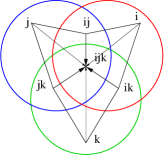
Figure 1: Intersections and their nerve.

After these preparations, define an element $\Sigma_{0}$ in $\mathsf{S}_{2,0}$ as

$$\Sigma_{0}=\sum_{i\in I}\mathrm{st}(v_{i})\cdot\Delta_{i}\,,$$

where

$$\mathrm{st}(v_{i})=\sum_{j,k:\Delta_{ijk}\neq 0}\epsilon_{ijk}\bigl{(}\Delta(v_{i},v_{ij},v_{ijk})-\Delta(v_{i},v_{ik},v_{ijk})\bigr{)}$$

is the star of the vertex $v_{i}$, and $\epsilon_{ijk}=\pm 1$ according to whether the order of the triple $i,j,k$ agrees the orientation or not, namely whether the order $ijk$ is the same as the cyclic (counterclockwise) order around the vertex $v_{ijk}$. Recall that $\Delta_{\tau}$ is the symbol corresponding to $U_{\tau}$, when considered as a generator in the abelian group generated by the nerve, as in A.2.2. Rewriting $\Sigma_{0}$ as

$$\sum_{i\in I}\mathrm{st}(v_{i})\cdot\Delta_{i}=\sum_{\langle i,j,k\rangle}\epsilon_{ijk}\biggl{\{} \bigl{(}\Delta(v_{i},v_{ij},v_{ijk})-\Delta(v_{i},v_{ik},v_{ijk})\bigr{)}\cdot\Delta_{i}$$

$$- \bigl{(}\Delta(v_{j},v_{ij},v_{ijk})-\Delta(v_{j},v_{jk},v_{ijk})\bigr{)}\cdot\Delta_{j}$$

$$+ \bigl{(}\Delta(v_{k},v_{ik},v_{ijk})-\Delta(v_{k},v_{jk},v_{ijk})\bigr{)}\cdot\Delta_{k}\biggr{\}},$$

where $\sum_{\langle i,j,k\rangle}$ means sum over triples of indices in $I$, its first differential is:

$$\partial^{\prime}\Sigma_{0} =\sum_{\langle i,j,k\rangle}\epsilon_{ijk}\bigl{\{}\Delta(v_{ik},v_{ijk})\cdot(\Delta_{k}-\Delta_{i})$$

$$\qquad-\Delta(v_{ij},v_{ijk})\cdot(\Delta_{j}-\Delta_{i})-\Delta(v_{jk},v_{ijk})\cdot(\Delta_{k}-\Delta_{j})\bigr{\}}$$

$$+\sum_{\langle i,j,k\rangle}\epsilon_{ijk}\bigl{\{}\Delta(v_{i},v_{ij})\cdot\Delta_{i}-\Delta(v_{i},v_{ik})\cdot\Delta_{i}-\Delta(v_{j},v_{ij})\cdot\Delta_{j}$$

$$\qquad+\Delta(v_{j},v_{jk})\cdot\Delta_{j}+\Delta(v_{k},v_{ik})\cdot\Delta_{k}-\Delta(v_{k},v_{jk})\cdot\Delta_{k}\bigr{\}}.$$

The last sum is easily seen to be zero, while the first can be rewritten as $\partial^{\prime\prime}\Sigma_{1}$ for the following element in $\mathsf{S}_{1,1}$:

$$\Sigma_{1}=\sum_{\langle i,j,k\rangle}\epsilon_{ijk}\bigl{\{}\Delta(v_{ik},v_{ijk})\cdot\Delta_{ik}-\Delta(v_{ij},v_{ijk})\cdot\Delta_{ij}-\Delta(v_{jk},v_{ijk})\cdot\Delta_{jk}\bigr{\}}$$

Again, computing the first differential gives

$$\partial^{\prime}\Sigma_{1} =\sum_{\langle i,j,k\rangle}\epsilon_{ijk}\bigl{\{}v_{ijk}\cdot(\Delta_{ik}-\Delta_{ij}-\Delta_{jk})\bigr{\}}$$

$$+\sum_{\langle i,j,k\rangle}\epsilon_{ijk}\bigl{\{}v_{ij}\cdot\Delta_{ij}-v_{ik}\cdot\Delta_{ik}+v_{jk}\cdot\Delta_{jk}\bigr{\}},$$

with the last sum being identically zero. The first term can be rewritten as $\partial^{\prime\prime}\Sigma_{2}$, where

$$\Sigma_{2}=-\sum_{\langle i,j,k\rangle}\epsilon_{ijk}v_{ijk}\cdot\Delta_{ijk}\,.$$

Finally, the total chain $\Sigma\equiv\Sigma_{0}+\Sigma_{1}-\Sigma_{2}$ is a cycle, $\partial\Sigma=0$, and we have the following expression for the representative of the fundamental class of $X$ in the double complex:

$$\Sigma =\sum_{\langle i,j,k\rangle}\epsilon_{ijk}\biggl{\{}\bigl{(}\Delta(v_{i},v_{ij},v_{ijk})-\Delta(v_{i},v_{ik},v_{ijk})\bigr{)}\cdot\Delta_{i}$$

$$\qquad\qquad\qquad-\bigl{(}\Delta(v_{j},v_{ij},v_{ijk})-\Delta(v_{j},v_{jk},v_{ijk})\bigr{)}\cdot\Delta_{j}$$

$$\qquad\qquad\qquad+\bigl{(}\Delta(v_{k},v_{ik},v_{ijk})-\Delta(v_{k},v_{jk},v_{ijk})\bigr{)}\cdot\Delta_{k}\biggr{\}}$$

$$+\sum_{\langle i,j,k\rangle}\epsilon_{ijk}\bigl{\{}\Delta(v_{ik},v_{ijk})\cdot\Delta_{ik}-\Delta(v_{ij},v_{ijk})\cdot\Delta_{ij}-\Delta(v_{jk},v_{ijk})\cdot\Delta_{jk}\bigr{\}}$$

$$+\sum_{\langle i,j,k\rangle}\epsilon_{ijk}v_{ijk}\cdot\Delta_{ijk}\,.$$

Remark A.2.2.

By taking the second augmentation, the total cycle $\Sigma$ maps to:

$$\sum_{\langle i,j,k\rangle}\epsilon_{ijk}\Delta_{ijk}\,,$$

which is the 2-cycle in the CW complex representing the combinatorics of the cover $\mathcal{U}$, and therefore the homology of $X$, in degree $p=2$.

Appendix B Acknowledgements

At the early stage of this work we appreciated useful discussions with J.L. Dupont and especially C.-H. Sah, who passed away in July 1997. His generosity of mind and enthusiasm made all our discussions special. He is deeply missed.

The work of L.T. was partially supported by the NSF grant DMS-98-02574.

References

• [1] L. Ahlfors, Lectures on Quasiconformal Mappings. Van Nostrand, 1966.
• [2] E. Aldrovandi, L.A. Takhtajan, Generating Functional in CFT and Effective Action for Two-Dimensional Quantum Gravity on Higher Genus Riemann Surfaces. Commun. Math. Phys. 188 (1997), 29–67.
• [3] O. Alvarez, Quantization and Cohomology. Commun. Math. Phys. 100 (1985), 279-309.
• [4] M. Artin, Grothendieck Topologies. Harvard Univ. Math. Dept. Lecture Notes, 1962.
• [5] M. Artin, A. Grothendieck, and J.-L. Verdier, Théorie des Topos et Cohomologie étale des Schemas. Lecture Notes in Mathematics 269, 270, 305, Springer-Verlag, 1972–1973.
• [6] M. Artin, B. Mazur, Étale homotopy. Springer Lecture Notes in Mathematics 100, Springer-Verlag, 1969.
• [7] R. Bott, L. Tu, Differential Forms in Algebraic Topology. Springer (Graduate Texts in Mathematics 82), 1982.
• [8] R. Brooks, W. Goldman, The Godbillon-Vey invariant of a transversely homogeneous foliation. Trans. AMS 286 (1984), 651–664
• [9] J.-L. Brylinsky, Loop Spaces, Characteristic Classes and Geometric Quantization. Prog. in Math. 107, Birkhäuser, 1993.
• [10] J.-L. Brylinsky, D. McLaughlin, The geometry of degree four characteristic classes and of line bundles on loop spaces I. Duke J. Math. 75 (1994), 603–632.
• [11] J.-L. Brylinsky, D. McLaughlin, The geometry of degree four characteristic classes and of line bundles on loop spaces II. Duke J. Math. 83 (1996), 105–139.
• [12] J.-L. Brylinski, Geometric construction of Quillen line bundles.In: Advances in Geometry J. Brylinski, R. Brylinski, V. Nistor, B. Tsygan, P. Xu, eds. Prog. in Math. 172 (1999).
• [13] P. Deligne, D. Freed, Classical Field Theory. In: Quantum Fields and Strings: A Course for Mathematicians, Vol. 1. P. Deligne, P. Etingof, D. Freed, L. Jeffrey, D. Kazhdan, J. Morgan, D. Morrison, E. Witten, eds. AMS and IAS (1999).
• [14] C. J. Earle, J. Eells, A fibre bundle description of Teichmüller theory. J. Diff. Geom. 3 (1969), 19–43.
• [15] H. Esnault, Characteristic classes of flat bundles, Topology 27 (1988), 323–352.
• [16] H. Esnault, E. Viehweg, Deligne-Beilinson cohomology. In: Beilinson’s Conjectures on Special values of $L$-Functions. M. Rapoport, N. Shappacher and P. Schneider, eds. Perspective in Math., Academic Press (1988)
• [17] L. Faddeev, S. Shatashvili, Realization of the Schwinger term in the Gauss law and the possibility of correct quantization of a theory with anomalies. Phys. Lett. B167 (1986), 225-228.
• [18] D. Freed, Higher Algebraic Structures and Quantization. Commun. Math. Phys. 159 (1994) 343–398
• [19] D. Freed, E. Witten, Anomalies in String Theory with D-Branes. arXiv:hep-th/9907189
• [20] K. Gawȩdzki, Topological actions in two-dimensional quantum field theory. In: Nonperturbative Quantum Field Theories. G. ’t Hooft, A. Jaffe, G. Mack, P.K. Mitter, R. Stora, eds. NATO Series vol. 185, Plenum Press (1988), 101–142.
• [21] Goldberg, Curvature and Homology. Dover, New York, 1982.
• [22] R.C. Gunning, Special coordinate coverings of Riemann surfaces. Math. Ann. 170 (1967), 67-86.
• [23] R.C. Gunning, Lectures on Riemann Surfaces. Princeton Univ. Press, 1966.
• [24] R.C. Gunning, Riemann Surfaces and Generalized Theta Functons. Springer-Verlag, 1976.
• [25] J. Hubbard, The monodromy of projective structures. In: Riemann Surfaces and Related Topics: Proceedings of the 1978 Sony Brook Conference. I. Kra, B. Maskit eds. Princeton Univ. Press, 1980.
• [26] I. Kra, Automorphic forms and Kleinian groups. Benjamin, 1972.
• [27] S. Lazzarini, Doctoral Thesis, LAPP Annecy-le-Vieux (1990) and references therein.
• [28] S. Mac Lane, Homology. Springer-Verlag, 1975. C.A. Weibel, An introduction to homomological algebra. Cambridge Univ. Press, 1994.
• [29] F. Magri, A simple model for the integrable Hamiltonian equation, J. Math. Phys. 19 (1978), 1156–1162.
• [30] S. Matsumoto, Some remarks on foliated $S^{1}$ bundles. Inv. Math. 90 (1987),
• [31] May, Simplicial objects in Algebraic Topology. Chicago Lectures in Mathematics, Univ. of Chicago Press, 1992.
• [32] Milne, Étale Cohomology. Princeton Mathematical Series 33 Princeton Univ. Press, 1980.
• [33] J. Milnor, On the existence of a connection with curvature zero. Comment. Math. Helv. 32 (1958), 215–223.
• [34] S. Nag, The complex analytic theory of Teichmüller spaces. Wiley Intersc., 1988.
• [35] A. M. Polyakov, Quantum gravity in two dimensions. Mod. Phys. Lett. A 2 (1987), 893–898.
• [36] G. Segal, Classifying Spaces and Spectral Sequences. Publ. IHES 34 (1968), 105–112.
• [37] F. Takens, A global version of the inverse problem of the calculus of variations. J. Diff. Geom. 14 (1979), 543-562.
• [38] A. Weil, Sur les théorèmes de de Rham. Comment. Math. Helv. 26 (1952), 119–145.
• [39] J.W. Wood, Bundles with totally disconnected structure group. Comment. Math. Helv. 46 (1971), 257–273.
• [40] R. Zucchini, A Polyakov action on Riemann surfaces. II. Commun. Math. Phys. 152 (1993), 269-298.
• [41] G. Zuckerman, Action principles and global geometry. In: Mathematical Aspects of String Theory. S.T. Yau ed., World Scientific Publishing, 1987.