The Anisotropic Averaged Euler Equations

Abstract

The purpose of this paper is to derive the anisotropic averaged Euler equations and to study their geometric and analytic properties. These new equations involve the evolution of a mean velocity field and an advected symmetric tensor that captures the fluctuation effects. Besides the derivation of these equations, the new results in the paper are smoothness properties of the equations in material representation, which gives well-posedness of the equations, and the derivation of a corrector to the macroscopic velocity field. The numerical implementation and physical implications of this set of equations will be explored in other publications.

1 Introduction

A fundamental problem in turbulent fluid dynamics is the difficulty in resolving the many spatial scales that are activated by the complicated nonlinear interactions. It is a challenge to produce models that capture the large scale flow, while correctly modeling the influence of the small scale dynamics. While there are many efforts in this direction, the goal of the present paper is to introduce a new method that is based on the combination of two basic ideas: the use of an ensemble averaging that represents a spatial sampling of material particles over small spatial scales, and the use of asymptotic expansions together with this averaging on the level of the variational principle.

Our approach is conceptually similar to the method of Reynolds averaging and Large Eddy Simulation techniques, but has the advantage of 1) not needing an additional closure model and 2) automatically providing a small scale corrector to the macroscopic flow field.

Our methodology has some interesting connections with the method of Optimal Prediction introduced by Chorin et al. [1999], which will be explored in future publications.

In the body of the paper we shall comment on a comparison between our approach and that of Chen et al. [1998] and Holm [1999], which produces different equations.

1.1 A Brief Review of the Euler and Isotropic Averaged Euler Equations

A Brief History.

There has been much recent interest in the averaged Euler equations for ideal fluid flow. In this paper we will focus on the geometry and analysis of a related set of equations, which we call the anisotropic averaged Euler equations. The original averaged Euler equations appear as a special isotropic case of the more general equations.

The isotropic averaged Euler equations on all of ${\mathbb{R}}^{n}$ first appeared in the context of an approximation to the Euler equations in Holm et al. [1998a] and some of its variational structure was developed in Holm et al. [1998b]; this variational structure retains the quadratic form of the variational structure for the original Euler equations, so that the equations can be viewed as describing a certain geodesic flow in a sense similar to the work of Arnold [1966] and Ebin and Marsden [1970].

Remarkably, these equations are mathematically identical to the well-known inviscid second grade fluids equations introduced by Rivlin and Erickson [1955]. The geometric analysis of these equations, including well-posedness and other analytic properties, was developed in Shkoller [1998, 2000] and Marsden et al. [2000]. These references also discuss the relation to the second-grade fluid literature.

In Oliver and Shkoller [2000], the link with the vortex blob method was established; therein, it was shown that the vortex blob numerical algorithm generates unique global weak solutions to the averaged Euler equations. These weak solutions induce a weak coadjoint action on the vector space of vorticity functions, modeled as the space of Radon measures. The existence of such a weak coadjoint action makes rigorous the formal constructions of Marsden and Weinstein [1983] on the geometry of point-vortex and vortex blob dynamics.

The works of Chen et al. [1998] and Holm [1999] formulated equations for the slow time dynamics of fluid motion by averaging over fast time fluctuations about the mean; that approach, founded on a Reynolds decomposition translated over the Lagrangian parcel, and the resulting system of equations, is different from our approach and from the results that we shall present. We give a few more details on the comparison in the body of the paper.

The Euler Equations as Geodesics and Notation.

It is well-known how to view the Euler equations as geodesics on the group of diffeomorphisms and that this view has concrete analytical advantages, due to the work of Arnold [1966] and Ebin and Marsden [1970]. In particular, this work shows that the equations define a smooth vector field (a spray) on the group of diffeomorphisms, that is, in Lagrangian (or material) representation. The reduction of the equations from material to spatial (Eulerian) representation may be viewed by the classical and general technique of Euler-Poincaré reduction (see Marsden and Ratiu [1999] and Holm et al. [1998b] for an exposition and further references) and this view is a helpful guide to understanding other fluid theories as well.

The geometric view of fluid mechanics, along with a careful understanding of the averaging process, will be basic to the present paper, so we briefly review the salient features of the theory for the reader’s convenience, and to establish notation.

Let $(M,g)$ be a $C^{\infty}$ compact, oriented $n$-dimensional Riemannian manifold with $C^{\infty}$ boundary (possibly empty). Of course open regions with smooth boundary in the plane or space are key examples. The Riemannian volume form associated with the metric $g$ is denoted $\mu$.

The Euler equations for the velocity field $u$ of an ideal, incompressible, homogeneous fluid moving on $M$ (such as a region $\Omega$ in $\mathbb{R}^{2}$ or $\mathbb{R}^{3}$) are

$$\frac{\partial u}{\partial t}+(u\cdot\nabla)u=-\nabla p$$ (1.1)

with the constraint $\operatorname{div}\,u=0$ and the boundary condition that $u$ is tangent to the boundary, $\partial M.$ The pressure $p$ is determined by the incompressibility constraint. The nonlinear term $(u\cdot\nabla)u$ is interpreted in the context of manifolds to be $\nabla_{u}u$, the covariant derivative of $u$ along $u$. In Euclidean coordinates, these equations are given as follows (using the summation convention for repeated indices):

$$\frac{\partial u^{i}}{\partial t}+u^{j}\frac{\partial u^{i}}{\partial x^{j}}=-\frac{\partial p}{\partial x^{i}}\,,$$

and on a Riemannian manifold (or in curvilinear coordinates in Euclidean space), the Euler equations take the following coordinate form:

$$\frac{\partial u^{i}}{\partial t}+u^{j}\frac{\partial u^{i}}{\partial x^{j}}+\Gamma^{i}_{jk}u^{j}u^{k}=-g^{ij}\frac{\partial p}{\partial x^{j}}\,,$$

where $g_{ij}$ are the components of the Riemannian metric $g$, $g^{ij}=[g_{ij}]^{-1}$, and $\Gamma^{i}_{jk}$ are the associated Christoffel symbols. Using covariant derivative notation, these coordinate equations read

$$\frac{\partial u^{i}}{\partial t}+u^{j}u^{i}_{\;;j}=-g^{ij}p_{,j}.$$

We let the flow of the time dependent vector field $u(t,x)$ be denoted by $\eta(t,x)$ so that

$$\frac{\partial}{\partial t}\eta(t,x)=u(t,\eta(t,x)),$$

with $\eta(0,x)=x$ for all $x$ in $M$. For each $t$, we denote the map $\eta(t,\cdot)$ by $\eta_{t}$ so that $\eta_{0}=e$, the identity map. Thus, the map $x\mapsto\eta_{t}(x)$ gives the particle placement field for the fluid. Because of the incompressibility, each map $\eta_{t}$ is volume preserving and is a diffeomorphism.

We shall be working with vector fields $u$ of Sobolev class $H^{s}$ for $s>(n/2)+1$ and, correspondingly, $\eta_{t}\in\mathcal{D}_{\mu}^{s}$, the group of $H^{s}$-volume preserving diffeomorphisms. If there is any danger of confusion, we shall write $\mathcal{D}_{\mu}^{s}(M)$ to indicate the underlying manifold $M$. See Ebin and Marsden [1970] and Shkoller [2000] for some basic properties of Hilbert class diffeomorphism groups for manifolds with boundary.

Arnold’s theorem on the Euler equations may be stated as follows: A time dependent velocity field $u$ satisfies the Euler equations iff the curve $\eta_{t}$ is a geodesic of the right invariant $L^{2}$-metric on $\mathcal{D}_{\mu}^{s}$.

This $L^{2}$-metric is defined as follows. The tangent space to $\mathcal{D}_{\mu}^{s}$ at the identity is identified with the space $\mathfrak{X}_{\operatorname{div}}^{s}$, the space of $H^{s}$ divergence free vector fields on $M$ that are tangent to the boundary $\partial M$. The right invariant $L^{2}$-metric is defined to be the weak Riemannian metric on $\mathcal{D}_{\mu}^{s}$ whose value at the identity is

$$\left\langle u,w\right\rangle_{L^{2}}=\int_{M}\left\langle u(x),w(x)\right\rangle_{x}\mu(x),$$

where we write the pointwise inner product as $\left\langle u(x),w(x)\right\rangle_{x}=g(x)(u(x),w(x))$, and the pointwise norm $|u(x)|^{2}=\left\langle u(x),u(x)\right\rangle_{x}$.

As we shall explain shortly, with the maturation of Euler-Poincaré theory, Arnold’s theorem becomes an easy consequence of more general and rather simple results.

Lie Derivative and Vorticity Form.

As is well-known, the Euler equations can be written in terms of Lie derivatives as

$$\frac{\partial u^{\flat}}{\partial t}+\pounds_{u}u^{\flat}=\mathbf{d}\left(\frac{1}{2}|u|^{2}-p\right)=-\mathbf{d}p^{\prime},$$ (1.2)

where $u^{\flat}$ is the one-form associated to the vector field $u$ via the metric, and $\pounds_{u}u^{\flat}$ denotes the Lie derivative of the one-form $u^{\flat}$ along $u$. Taking the exterior derivative of (1.2) gives the familiar advection equation for vorticity:

$$\frac{\partial\omega}{\partial t}+\pounds_{u}\omega=0,$$

where $\omega=\mathbf{d}u^{\flat}$ is the vorticity, thought of as a two-form. In 2D, $\omega$ is identified with a scalar and is traditionally thought of as the 2D-curl of the velocity field, while in 3D, $\omega$ may be identified (using the volume-form $\mu$) with a vector field which is traditionally obtained by taking the curl of $u$.

The vorticity equation is the infinitesimal version of the following advection property:

$$\omega_{t}=(\eta_{t})_{\ast}\omega_{0}.$$

Of course in two dimensions, this gives the usual advection of vorticity as a function, while in three (or higher) dimensions, the advection is understood in terms of advection of two-forms.

The Euler equations have both an interesting Hamiltonian structure in terms of Poisson brackets (a Lie-Poisson bracket) and a variational structure. In this paper we shall be working primarily with the variational structure; the Hamiltonian structure, along with references to the literature may be found in Marsden and Weinstein [1983], Arnold and Khesin [1998] and Marsden and Ratiu [1999].

Lagrangian and Variational Form.

The Lagrangian is given by the total kinetic energy of the fluid; in spatial representation, this Lagrangian is

$$L(u)=\frac{1}{2}\int_{M}|u(x)|^{2}\mu.$$ (1.3)

The corresponding (unreduced) Lagrangian on $T\mathcal{D}_{\mu}^{s}$ is given by

$$\mathcal{L}(\eta,\dot{\eta})=\frac{1}{2}\int_{M}g(\eta(x))(\dot{\eta}(x),\dot{\eta}(x))\mu.$$ (1.4)

Hamilton’s principle on $\mathcal{D}_{\mu}^{s}$ applied to the Lagrangian $\mathcal{L}$ gives geodesics on this group. Euler-Poincaré reduction techniques (see Marsden and Ratiu [1999]) show that this variational principle reduces to the following principle in terms of Eulerian velocities:

$$\delta\int_{a}^{b}L(u)\,dt=0,$$

which should hold for all variations $\delta u$ of the form

$$\delta u=\dot{w}+[u,w],$$

where $w$ is a time dependent vector field (representing the infinitesimal particle displacement) vanishing at the temporal endpoints. Here, $[w,u]$ denotes the usual Jacobi–Lie bracket of vector fields. One readily checks that this reduced principle yields the standard Euler equations. This simple computation is the heart of Arnold’s theorem.

Analytical Issues.

While the Eulerian (spatial) representation has been emphasized in most analytic studies of the Euler equations, fluid motion viewed on the Lagrangian (material) side has some distinct advantages. For example, Ebin and Marsden [1970] proved that the flow, solving the Euler equations, on the volume-preserving diffeomorphism group $\mathcal{D}_{\mu}^{s}$, $s>n/2+1$, is smooth in time. They derived a number of interesting consequences from this result, including theorems on the convergence of solutions of the Navier-Stokes equations to solutions of the Euler equations as the viscosity goes to zero when $M$ has no boundary. In addition, Marchioro and Pulvirenti [1994] analyzed the Lagrangian flow map to establish sharp well-posedness of the 2D Euler equations and prove convergence of the vortex blob algorithm. In many cases, the Lagrangian framework is, in fact, the more natural setting to study the behavior of solutions, and we shall emphasize this point of view.

1.2 The Averaged Euler Equations

The Isotropic Averaged Euler Equations.

Let $\alpha$ be a positive constant. In Euclidean space and in Euclidean coordinates, the isotropic averaged Euler equations (inviscid second-grade fluids equations) read:

$$\frac{\partial v^{i}}{\partial t}+u^{j}\frac{\partial v^{i}}{\partial x^{j}}-\alpha^{2}\left[\frac{\partial u^{j}}{\partial x^{i}}\right]\Delta u_{j}=-\frac{\partial p}{\partial x^{i}}\,,$$

where $v=u-\alpha^{2}\Delta u$ and $\Delta$ denotes the componentwise Laplacian, and there is a summation over repeated indices (in Euclidean coordinates, as is common, we make no distinction between indices up or down). While there are several choices, the no slip boundary conditions $u=0$ are often used for this model.

Rate of Deformation Tensor.

One of the interesting things that comes out of a careful derivation of the equations is the natural occurence of the rate of deformation tensor, which is defined by

$$\operatorname{Def}u=\frac{1}{2}\left(\nabla u+(\nabla u)^{T}\right)$$

which we write in coordinates as:

$$\left(\operatorname{Def}u\right)^{i}_{\;j}=\frac{1}{2}\left(u^{i}_{\;;j}+u^{j}_{\;;i}\right).$$

We also let $\operatorname{Def}u^{\flat}=\frac{1}{2}\left[\nabla u^{\flat}+(\nabla u^{\flat})^{T}\right]$ which we write in coordinates as

$$D_{ij}=\big{(}\operatorname{Def}u^{\flat}\big{)}_{ij}=\frac{1}{2}\big{(}u_{i;j}+u_{j;i}\big{)}.$$

Note that this is exactly the Lie derivative of the metric tensor; that is, $\operatorname{Def}u^{\flat}=\pounds_{u}g$, which is sometimes called the Killing tensor.

Smoothness Properties.

Results on smoothness of the Lagrangian flow map for the averaged Euler equations were given in Shkoller [1998] on compact boundaryless Riemannian manifolds, and in Marsden et al. [2000] on compact Euclidean domains. The problem of how to formulate this system on compact Riemannian manifolds with boundary was solved in Shkoller [2000]; the equations take the form

$$\partial_{t}(1-\alpha^{2}\Delta_{r})u+\nabla_{u}(1-\alpha^{2}\Delta_{r})u-\alpha^{2}(\nabla u)^{t}\cdot\Delta_{r}u=-\operatorname{grad}p,$$

together with the constraint $\operatorname{div}u=0,$ and with appropriate initial conditions $u(0)=u_{0}$, as well as boundary conditions. The symbol $\Delta_{r}$ is the operator $\operatorname{Def}^{*}\operatorname{Def}$ acting on divergence-free vector fields, where $\operatorname{Def}^{*}$ is the $L^{2}$ formal adjoint of the (rate of) deformation operator $\operatorname{Def}$. Explicitly,

$$\Delta_{r}=-(d\delta+\delta d)+2\operatorname{Ric}.$$ (1.5)

As with the usual Euler equations, the function $p$ is determined from the incompressibility condition.

Lie Derivative Form—The Isotropic Equations.

The averaged Euler equation can be neatly written in terms of Lie derivatives:

$$\partial_{t}v^{\flat}+\pounds_{u}v^{\flat}=-dp,$$ (1.6)

where $v^{\flat}=(1-\alpha^{2}\Delta_{r})u^{\flat}$.

The Anisotropic Averaged Euler Equations.

These equations, which are the main subject of the present paper, and which will be derived in §3.2, will now be stated. The basic variables that are evolving in the anisotropic averaged Euler equations are the macroscopic velocity field $u$ and a symmetric tensor field $F$ on $M$; the tensor field $F$ will be interpreted as the contravariant spatial fluctuation tensor and it will keep track of the anisotropy of the fluid deviations from the macroscopic flow. These equations also depend on a choice of length scale $\alpha$.

It is convenient to define the linear operator ${\mathcal{C}}:\mathfrak{X}_{\operatorname{div}}^{s}\cap H^{1}_{0}\rightarrow H^{s-2}$, $s\geq 1$, by

$$\mathcal{C}u:=\operatorname{Div}\left[C:\nabla u^{\flat}\right],$$

where $\flat$ is the map from vector fields to one-forms associated with the metric $g$, and the fourth-rank symmetric positive tensor $C$ is the symmetrization of the tensor $F\otimes g^{-1}$, given in local coordinates by

$$C^{ijkl}={\frac{1}{4}}\left(F^{lj}g^{ik}+f^{kj}g^{il}+F^{li}g^{jk}+F^{ki}g^{jl}\right).$$

With this notation, the anisotropic averaged Euler equations on manifolds are

$$\partial_{t}(1-\alpha^{2}\mathcal{C})u +\nabla_{u}(1-\alpha^{2}\mathcal{C})u-\alpha^{2}[\nabla u]^{t}\cdot\mathcal{C}u+2\alpha^{2}F:\left[\nabla(\operatorname{Def}u^{\flat})^{2}\right]^{\sharp}$$

$$-4\alpha^{2}\operatorname{Div}\left(\left(\operatorname{Def}u\right)^{2}\cdot F\right)=-\operatorname{grad}p,$$

together with the advection equation

$$\partial_{t}F+\pounds_{u}F=0,$$

the incompressibility constraint $\text{div }u=0$, initial data $u(0)=u_{0}$ and $F(0)=F_{0}$, and the Dirichlet boundary condition $u=0$.

Lie Derivative Form—Anisotropic Equations.

The anisotropic averaged Euler equations can also be written using Lie derivatives as

$$\partial_{t}v^{\flat}+\pounds_{u}v^{\flat}+\left[2\alpha^{2}F:\left[\nabla(\operatorname{Def}u^{\flat})^{2}\right]^{\sharp}-4\alpha^{2}\operatorname{Div}\left(\left(\operatorname{Def}u\right)^{2}\cdot F\right)\right]^{\flat}=-dp,$$ (1.7)

where $v^{\flat}=(1-\alpha^{2}\mathcal{C}^{\flat})u^{\flat}$, where ${\mathcal{C}}^{\flat}u^{\flat}=\text{Div}[C:\nabla u^{\flat}]^{\flat}$.

Coordinate Form.

In local coordinates, the anisotropic averaged Euler equations become

$$\partial_{t}\left(u^{i}-\alpha^{2}[C^{ijkl}u_{k},_{j}],_{l}\right)+\left(u^{i}-\alpha^{2}[C^{ijkl}u_{k},_{j}],_{l}\right),_{m}u^{m}-\alpha^{2}u_{m},_{i}[C^{mjkl}u_{k},_{j}],_{l}$$

$$\qquad+2\alpha^{2}F^{kj}[D_{km}g^{mn}D_{nj}],_{i}-4\alpha^{2}[F^{kj}D_{im}g^{mn}D_{nj}],_{k}$$

$$\qquad\quad=-p,_{i}$$

together with the advection equation

$$\partial_{t}F^{ij}+F^{ij},_{k}u^{k}-F^{kj}u^{i},_{k}-F^{ik}u^{j},_{k}=0,$$

with the constraint $u^{i}_{\;,i}=0$, given initial conditions $u^{i}(0)=u^{i}_{0}$, and with the no-slip conditions $u^{i}=0$ on the boundary. If the metric $g$ is not the Euclidean metric $\delta_{ij}$, then the partial derivatives above should be interpreted as arising from the Levi-Civita covariant derivative associated to $g$.

1.3 Outline of the Main Results.

The main results of the present work are as follows:

1. We derive, in a systematic way, the first order averaged Lagrangian given in coordinates by

   $$L^{\alpha}_{1}(u,F)=\frac{1}{2}\int_{M}\left\{g_{ik}u^{i}u^{k}+2\alpha^{2}g^{ik}F^{jl}D_{ij}D_{kl}\right\}[\text{det }g]^{\frac{1}{2}}dx.$$

   and, using the calculus of variations, derive the associated anisotropic averaged Euler equations as the corresponding Euler-Poincaré equations. The Euler-Poincaré technique was also used in Holm [1999], but the Lagrangian and associated equations are different. In particular, the principles and philosophy governing the derivation of the Lagrangian are completely different.

2. We show that the equations are well posed; in fact, we show more, namely that the corresponding Lagrangian flow map is smooth in time in the appropriate Sobolev topology.

3. Another important achievement is that while the macroscopic velocity field $u$ is computed on spatial scales larger than $\alpha$, we are able to obtain a corrector for this macroscopic field to order $\alpha^{2}$. This is done in §4.2 and is similar to what one does in the theory of homogenization.

2 The Derivation

2.1 Introduction

This section presents a new method for constructing models of hydrodynamics which takes into account the fundamental idea that a fluid particle is not a point, but rather a collection of points forming a representative sampling. Our approach is founded upon a certain type of Lagrangian ensemble averaging performed at the level of the variational principle. A similar idea on the level of the equation itself, as opposed to the variational principle, was used by Barenblatt and Prostokishin [1993] for deriving models of damage propagation.

Naive Averaging Does not Work.

We first explain why the naive approach to spatially averaging a quadratic Lagrangian or Hamiltonian does not suffice. As a simple example, consider the Lagrangian on scalar functions on $\mathbb{R}^{n}$ given by $L(u)=\frac{1}{2}\int_{\mathbb{R}^{n}}u^{2}(x)dx$ and for a given positive constant $\alpha$, define a new averaged Lagrangian by

$$L^{\alpha}(u)=\int_{\mathbb{R}^{n}}\frac{1}{|B(x,\alpha)|}\int_{B(x,\alpha)}u^{2}(z)dzdx$$

which is obtained from $L$ by averaging the original Lagrangian over balls of radius $\alpha$. Here $B(x,\alpha)$ denotes the ball of radius $\alpha$ about the point $x$ in $\mathbb{R}^{n}$ and $|B(x,\alpha)|$ denotes its volume.

Taylor expanding the integrand about $x$ and then integrating by parts yields cancellation of all but the zeroth-order term, thus reproducing exactly the original Lagrangian $L$. This is to be expected since the quadratic nonlinearity is rather weak, and since absolutely no information concerning the local spatial structure of the continuum is being provided. The latter issue is of fundamental importance and is the foundation upon which we shall build our theory.

2.2 The Averaging Construction.

To implement our construction, we will average over an ensemble of Lagrangian fluctuation maps. We will now proceed to develop this formalism.

Fuzzying the Lagrangian Flow.

Let $(M,g)$ be a $C^{\infty}$ compact, oriented $n$-dimensional Riemannian manifold with $C^{\infty}$ boundary (possibly empty). We consider a two-parameter family of volume-preserving diffeomorphisms $\xi^{\epsilon,\theta}$ of $M$ depending on a “radial” component $\epsilon\in[-\alpha/2,\alpha/2]$, $\alpha>0$, and an “angular” component $\theta\in S^{n-1}_{+}$, where $S^{n-1}_{+}$ denotes the upper hemisphere of the unit sphere $S^{n-1}$ in ${\mathbb{R}}^{n}$. In case $M$ has nonempty boundary, we embed $M$ into its double $\tilde{M}$ and consider this two-parameter family defined on $\tilde{M}$; in this case, $\xi^{\epsilon,\theta}$ need not leave $\partial M$ invariant. This fact will be important later for certain ellipticity properties.

The parameterization is chosen such that

$$\begin{array}[]{c}\xi^{0,\theta}(t,x)=x,\\ \text{dist}(x,\xi^{\epsilon,\theta}(x))<|\epsilon|\end{array}$$

for all $\epsilon\in[-\alpha/2,\alpha/2]$, all $t$, and $\theta\in S^{n-1}_{+}$. We define the infinitesimal fluctuation vector by

$$\xi^{\prime}(\theta,t,x)=\left.{\frac{d}{d\epsilon}}\right|_{\epsilon=0}\xi^{\epsilon,\theta}(t,x),$$

a vector field depending on the parameter $\theta$ and time $t$.

For each time $t$, the Lagrangian flow map $\eta_{t}$, where $\eta_{t}(x)=\eta(t,x)$, associated with a solution of the Euler equations is a volume-preserving diffeomorphism of $M$ which maps fluid particles $x\in M$ to $\eta_{t}(x)\in M$. Motivated by the idea that a particle in a continuum should really be regarded as a representative of a sample of particles over a region, we define the $\xi^{\epsilon,\theta}_{t}$-perturbed particle placement field by

$$\eta^{\epsilon,\theta}_{t}(x)=(\xi^{\epsilon,\theta}_{t})^{-1}\circ\eta_{t}(x)$$ (2.1)

for all $\epsilon\in[-\alpha/2,\alpha/2]$ and $\theta\in S^{n-1}_{+}$. The family of maps $\eta^{\epsilon,\theta}_{t}$ is called the fuzzy flow. For each $\epsilon$, $\theta$, and $t$, the map $\eta^{\epsilon,\theta}_{t}:M\rightarrow M$ is a volume-preserving diffeomorphism of the fluid container. Note that at $\epsilon=0$, $\eta^{0,\theta}_{t}=\eta_{t}$ for all $\theta\in S^{n-1}_{+}$.

We take $\eta_{t}\in\mathcal{D}_{\mu}^{s}(M)$ and $\xi_{t}^{\epsilon,\theta}\in\mathcal{D}_{\mu}^{\infty}(\tilde{M})$ so that $\eta_{t}^{\epsilon,\theta}\in\mathcal{D}_{\mu}^{s}(\tilde{M})$. See §1.1 for the definition of the group $\mathcal{D}_{\mu}^{s}$.

Decomposition of the Spatial Velocity Field.

Our goal is to derive the Eulerian velocity field $u^{\epsilon,\theta}_{t}$ corresponding to the $\xi^{\epsilon,\theta}_{t}$-perturbed particle placement field $\eta^{\epsilon,\theta}_{t}$, and define a new Lagrangian by averaging the velocity $u^{\epsilon,\theta}_{t}$ over the radial parameter $\epsilon$ and the angular coordinate $\theta$. We shall proceed with this averaging process as follows: we begin by defining the Eulerian vector fields associated with our three Lagrangian maps. Let

$$\partial_{t}\eta(t,x) =u(t,\eta(t,x)),$$

$$\partial_{t}\xi^{\epsilon,\theta}(t,x) =w^{\epsilon,\theta}(t,\xi^{\epsilon,\theta}(t,x)),$$

$$\partial_{t}\eta^{\epsilon,\theta}(t,x) =u^{\epsilon,\theta}(t,\eta^{\epsilon,\theta}(t,x)).$$

Differentiating the Lagrangian decomposition (2.1) with respect to time $t$, we obtain the spatial velocity decomposition

$$u^{\epsilon,\theta}(t,x)=\left\{{\xi^{\epsilon,\theta}}^{*}(u-w^{\epsilon,\theta})\right\}(t,x),$$ (2.2)

where the notation ${\xi^{\epsilon,\theta}}^{*}$ denotes the pullback by the map $\xi^{\epsilon,\theta}$. We can also write this decomposition using the push-forward notation via the relation $\big{(}{\xi^{\epsilon,\theta}_{t}}\big{)}^{\ast}={\big{(}\xi^{\epsilon,\theta}_{t}\big{)}^{-1}}_{*}$, so that the action on a vector field $v$ is given by

$$\big{(}{\xi^{\epsilon,\theta}_{t}}\big{)}^{\ast}v=T(\xi^{\epsilon,\theta}_{t})^{-1}\circ v\circ\xi^{\epsilon,\theta}_{t},$$

where we use the symbol $T$ to denote the tangent map (which is locally represented by the matrix of partial derivatives). Thus, the decomposition (2.2) may be equivalently written as

$$u^{\epsilon,\theta}(t,x)=T(\xi^{\epsilon,\theta}_{t})^{-1}(x)\circ\left(u(t,\xi^{\epsilon,\theta}_{t}(x))-w^{\epsilon,\theta}(t,\xi^{\epsilon,\theta}_{t}(x))\right),$$ (2.3)

where, again, $u^{\epsilon,\theta}(t,x)$ is the Eulerian spatial velocity field corresponding to the fuzzy flow $\eta^{\epsilon,\theta}_{t}$.

Comments on the Nature of the Decomposition.

The Lagrangian decomposition (2.1) which “fuzzies” the Lagrangian flow map yields the decomposition (2.3) for the corresponding Eulerian variables which is of a hybrid Lagrangian-Eulerian type. The Lagrangian characteristics of this decomposition are encompassed in the presence of the purely Lagrangian fluctuation maps $\xi^{\epsilon,\theta}_{t}$, and it is indeed the presence of this Lagrangian term in (2.3) which allows us to proceed with an asymptotic expansion which is both philosophically and mathematically different from the “naive” expansion we discussed earlier. We should also emphasize that without this Lagrangian aspect, the decomposition (2.3) would reduce to the usual additive (Reynolds) decomposition of spatial velocity fields into their mean and fluctuating parts, which does not reflect the fuzzyness of the Lagrangian flow map.

Our approach should also be contrasted with the approach taken by Chen et al. [1998] and Holm [1999]. In those papers, the decomposition

$$\eta^{\sigma}(t,x)=\eta(t,x)+\sigma(t,\eta(t,x)),$$

is made, where $\sigma(t,x)$ is a fluctuation vector field, and $\eta^{\sigma}(t,x)$ is a perturbed Lagrangian trajectory of the reference element $x$. This decomposition is intrinsically problematic, in that a material vector field $\sigma(t,\eta(t,\cdot))$ is being added to a volume-preserving diffeomorphism $\eta(t,\cdot)$. As a consequence, the perturbed trajectory $\eta^{\sigma}(t,x)$ does not come from a volume-preserving diffeomorphism of the fluid container, that is, $\eta^{\sigma}(t,\cdot)$ is not a volume-preserving map.

The Averaged Lagrangian.

We define the averaged Lagrangian $L^{\alpha}$ by

$$L^{\alpha}(u) ={\frac{1}{2}}\int_{M}\frac{1}{\alpha}\int_{-\alpha/2}^{\alpha/2}\int_{S^{n-1}_{+}}\langle u^{\epsilon,\theta}(t,x),u^{\epsilon,\theta}(t,x)\rangle d\epsilon\ \nu(\theta)\ \mu(x)$$

$$={\frac{1}{2}}\int_{M}\frac{1}{\alpha}\int_{-\alpha/2}^{\alpha/2}\int_{S^{n-1}_{+}}\left|{\xi^{\epsilon,\theta}}^{*}(u-w^{\epsilon,\theta})(t,x)\right|^{2}d\epsilon\ \nu(\theta)\ \mu(x),$$

where $\mu$ is the Riemannian volume form on $M$, and $\nu$ is the induced Riemannian volume form on $S^{n-1}_{+}$, the upper hemisphere of the unit sphere $S^{n-1}$ in ${\mathbb{R}}^{n}$.

Comments on the Nature of the Fuzzying Operation.

By using the upper hemisphere $S^{n-1}_{+}$ and integrating from $-\alpha/2$ to $\alpha/2$, we are tacitly assuming that there is a hyperplane of symmetry in the $\theta$-parameter space. This is not a restriction even near the boundary, as the hyperplane of symmetry can always be chosen orthogonal to the boundary and the maps $\xi^{\epsilon,\theta}_{t}$ can be chosen to be symmetric about this hyperplane with respect to the radial parameter $\epsilon$.

The reader should keep in mind that the variables $\theta$ and $\epsilon$ parameterize possible families of maps and are not to be confused with spatial spheres in the flow itself. We are averaging over these families of maps and not literally over spatial regions. A representative of the family of fluctuation maps $\xi^{\epsilon,\theta}$ in the two dimensional case and near a boundary is shown in Figure 2.1.

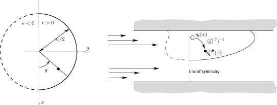
Figure 2.1: An example of a perturbing map $\xi^{\epsilon,\theta}_{t}$; its inverse takes the flow point $\eta_{t}(x)$ to the perturbed flow point $\eta^{\epsilon,\theta}_{t}(x)$. The parameter space for $(\epsilon,\theta)$ and the symmetry plane is shown on the left.

The internal structure behind the fuzzyness of the macroscopic Lagrangian flow is completely encoded in the fluctuation maps $\xi^{\epsilon,\theta}_{t}$.

The zeroth-order assumption that these maps are simply the identity map leads to the zeroth-order Lagrangian $L^{\alpha}_{0}$ which is exactly equal to the Lagrangian $L$ given in (1.3) and thus produces the usual Euler equations of hydrodynamics as the continuum model. We proceed to obtain the first order correction to this model which accounts for the spatial fluctuations.

Asymptotic Expansion.

We Taylor expand $u^{\epsilon,\theta}$ in $\epsilon$ about $\epsilon=0$ to obtain

$$u^{\epsilon,\theta}(t,x)={\xi^{\epsilon,\theta}_{t}}^{*}(u_{t}-w^{\epsilon,\theta}_{t})(x)=u_{t}(x)+\epsilon\pounds_{\xi^{\prime}(\theta,t,x)}u_{t}(x)-\epsilon\dot{\xi}^{\prime}(\theta,t,x)+O(\epsilon^{2}),$$ (2.4)

where the overdot means the time derivative. This follows from the definition of the Lie derivative, the fact that $w^{\epsilon,\theta}=\partial_{t}\xi^{\epsilon,\theta}_{t}\circ\xi^{\epsilon,\theta}_{t}$, and that $\left.\xi^{\epsilon,\theta}_{t}\right|_{\epsilon=0}=e$. Using the zero-torsion condition on the Levi-Civita covariant derivative, $\pounds_{{\xi}^{\prime}}u=\nabla_{{\xi}^{\prime}}u-\nabla_{u}{\xi}^{\prime}$, and suppressing the dependence on $t$ and $x$, we get

$$u^{\epsilon,\theta}=u+\epsilon(\nabla u\cdot\xi^{\prime}(\theta)-\nabla\xi^{\prime}(\theta)\cdot u-\dot{\xi}^{\prime}(\theta))+O(\epsilon^{2})$$

or, in index notation,

$${u^{\epsilon}}^{i}=u^{i}+\epsilon\left(u^{i}_{\;;j}\xi^{j}(\theta)-\xi^{i}_{\;;j}(\theta)u^{j}-\dot{\xi}^{i}(\theta)\right)+O(\epsilon^{2}),$$

where

$$u=u^{i}\partial_{i},\ \ \ \xi^{\prime}=\xi^{i}\partial_{i}\quad\text{and}\quad\nabla u\cdot\xi^{\prime}=u^{i}_{\;;j}\xi^{j}\partial_{i}.$$

In order to proceed, we make the first-order Taylor Hypothesis that the infinitesimal fluctuation vector $\xi^{\prime}$ is frozen, as a one-form, into the fluid so that its Lie transport vanishes; namely,

$$(\dot{\xi}^{\prime}_{t})^{\flat}+\pounds_{u}(\xi^{\prime})^{\flat}=0.$$ (2.5)

We again express the Lie derivative of the $1$-form field $(\xi^{\prime})^{\flat}$ in terms of the covariant derivative to obtain, in index notation,

$$\dot{\xi}_{i}+u^{j}_{;i}\xi_{j}+\xi_{i;j}u^{j}=0.$$

From this hypothesis, the $O(\epsilon)$ term in the Taylor expansion (2.4) is

$$u_{i;j}-\xi_{i;j}u^{j}+u^{j}_{;i}\xi_{j}+\xi_{i;j}u^{j} =u_{i;j}\xi^{j}+u^{j}_{;i}\xi_{j}$$

$$=u_{i;j}\xi^{j}+u_{j;i}\xi^{j}=2\operatorname{Def}u^{\flat}\cdot\xi^{\prime}(\theta).$$

It follows that

$$u^{\epsilon,\theta}=(\xi^{\epsilon,\theta})^{\ast}(u-w^{\epsilon})=u+2\epsilon\operatorname{Def}u\cdot\xi^{\prime}(\theta)+O(\epsilon^{2}).$$ (2.6)

Substitution of (2.6) into the averaged Lagrangian $L^{\alpha}$ yields

$$L^{\alpha}(u)={\frac{1}{2}}\int_{M}{\frac{1}{\alpha}}\int_{S^{n-1}_{+}}\int_{-\alpha/2}^{\alpha/2}\left[|u(x)|^{2}+2\epsilon\langle u(x),\operatorname{Def}u(x)\cdot\xi^{\prime}(x,\theta)\rangle\right.$$

$$\qquad\qquad\left.+\;4\epsilon^{2}|\operatorname{Def}u(x)\cdot\xi^{\prime}(x,\theta)|^{2}+O(\epsilon^{3})\right]d\epsilon\ \nu(\theta)\ \mu(x).$$ (2.7)

An important point about this expression is the following: There is no contribution from the term $\langle u,O(\epsilon^{2})\rangle$ to the energy at order $O(\epsilon^{2})$. In fact, the $O(\epsilon^{2})$ term in (2.6) has the form $O(\epsilon^{2})=\epsilon^{2}\left(\dot{\xi^{\prime\prime}}+R\right)$, where

$$\dot{\xi^{\prime\prime}}:=\frac{d}{dt}\left.\frac{d^{2}\xi}{d\epsilon^{2}}\right|_{\epsilon=0}.$$

However, $\xi^{\prime\prime}$ is an independent field and must have its own dynamics specified. We assume that this dynamics is chosen so that $\dot{\xi}^{\prime\prime}+R$ is $O(\epsilon)$ and so the a priori $O(\epsilon^{2})$-term in (2.6) is in fact $O(\epsilon^{3})$.

Integrating (2.7) in $\epsilon$, rescaling $\alpha\mapsto\sqrt{\alpha/6}$, and defining the symmetric rank-$2$ contravariant spatial fluctuation tensor (indices up) $F$ by

$$F(x)=\int_{S^{n-1}_{+}}\xi^{\prime}(x,\theta)\otimes\xi^{\prime}(x,\theta)\nu(\theta),$$

we obtain the first-order averaged Lagrangian

$$L^{\alpha}_{1}(u,F) ={\frac{1}{2}}\int_{M}\int_{S^{n-1}_{+}}\left[|u|^{2}+2\alpha^{2}|\operatorname{Def}u\cdot\xi^{\prime}(x,\theta)|^{2}\right]\nu(\theta)\ \mu(x)$$

$$={\frac{1}{2}}\int_{M}\left[|u(x)|^{2}+2\alpha^{2}\langle F(x)\circ\operatorname{Def}u(x),\operatorname{Def}u(x)\rangle\right]\mu(x)$$

$$={\frac{1}{2}}\int_{M}\left\{|u(x)|^{2}+2\alpha^{2}\left[g(x)\otimes F(x)\right]:\left[\operatorname{Def}u(x)\otimes\operatorname{Def}u(x)\right]\right\}\mu(x).$$ (2.8)

In coordinate notation, the first-order averaged Lagrangian takes the form

$$L^{\alpha}_{1}(u,F)=\frac{1}{2}\int_{M}\left\{g_{ik}u^{i}u^{k}+2\alpha^{2}g_{ik}F^{jl}[\operatorname{Def}u]^{i}_{j}[\operatorname{Def}u]^{k}_{l}\right\}[\text{det }g]^{\frac{1}{2}}dx.$$

The first-order averaged Lagrangian $L^{\alpha}_{1}$ is a function of the macroscopic Eulerian velocity field $u$ and the contravariant spatial fluctuation tensor $F$.

The Isotropic Case.

In the case that the fluctuation tensor is isotropic so that

$$F(x)=g^{-1}(x),$$

the isotropic first-order averaged Lagrangian $L^{\alpha}_{1,\text{iso}}$ is given by

$$L^{\alpha}_{1,{\rm iso}}(u)={\frac{1}{2}}\int_{M}\left[|u(x)|^{2}+2\alpha^{2}|\operatorname{Def}u(x)|^{2}\right]\mu(x).$$

In this special case, the Lagrangian depends only on the Eulerian velocity field $u$ and no semi-direct product theory is required; in fact, the standard Euler-Poincaré theory for reduced Lagrangian variational principals may be invoked to obtain the isotropic averaged Euler equations as

$$\begin{array}[]{c}\partial_{t}(1-\alpha^{2}\Delta_{r})u+\nabla_{u}(1-\alpha^{2}\Delta_{r})u-\alpha^{2}(\nabla u)^{t}\cdot\Delta_{r}u=-\operatorname{grad}p,\\ \text{div }u=0,\ \ u(0)=u_{0},\\ \end{array}$$ (2.9)

where $\Delta_{r}=-(d\delta+\delta d)+2\operatorname{Ric}$ (see Shkoller [2000]). As we stated above, the equations (2.9) are precisely the equations of inviscid second-grade non-Newtonian fluids, and exactly coincide with Chorin’s vortex blob algorithm when a particular choice of smoothing kernel is used (see Oliver and Shkoller [2000]). In the case that $M$ is a manifold without boundary, the incompressibility of the fluid allows us to replace the term $2\alpha^{2}|\operatorname{Def}u|^{2}$ with $\alpha^{2}|\nabla u|^{2}$ in (2.8), and still obtain the identical evolution equations as in (2.9); however, for domains with boundary it is essential to retain the strain tensor $\operatorname{Def}u$ in the Lagrangian so as to obtain the natural boundary conditions which ensure ellipticity of the operator $(1-\alpha^{2}\Delta_{r})$.

3 The Variational Principle and Semidirect products

We shall next explain the sense in which the Lagrangian $L^{\alpha}_{1}(u,F)$ defined in (2.8), a function of spatial variables, can be obtained from a Lagrangian defined in material variables. This will be done via an Euler-Poincaré procedure, which involves the group $\mathcal{D}_{\mu,D}^{s}\,\circledS\,C^{\infty}(T^{2,0}(M))$, the semi-direct product of the volume-preserving diffeomorphism group $\mathcal{D}_{\mu,D}^{s}$ (with Dirichlet boundary conditions) and the smooth sections of the vector bundle $T^{2,0}(M)$, consisting of second-rank contravariant symmetric tensors. Before proceeding to our specific example, we shall digress briefly to explain the general theory.

3.1 Lagrangian Semidirect Product Theory.

The General Set Up.

Let $V$ be a vector space and assume that the Lie group $G$ acts linearly on the right on $V$ (and hence $G$ also acts on its dual space $V^{\ast}$). In the case that the vector space $V$ consists of sections of a vector bundle $E$, $V^{*}$ will denote the sections of the dual bundle $E^{*}$. The semidirect product $S=G\,\circledS\,V$ is the Cartesian product $S=G\times V$ whose group multiplication is given by

$$(g_{1},v_{1})(g_{2},v_{2})=(g_{1}g_{2},v_{2}+v_{1}g_{2}),$$ (3.1)

where the action of $g\in G$ on $v\in V$ is denoted simply as $vg$. The Lie algebra of $S$ is the semidirect product Lie algebra, $\mathfrak{s}=\mathfrak{g}\,\circledS\,V$, whose bracket is

$$[(\psi_{1},v_{1}),(\psi_{2},v_{2})]=([\psi_{1},\psi_{2}],\,v_{1}\psi_{2}-v_{2}\psi_{1}),$$ (3.2)

where we denote the induced action of $\mathfrak{g}$ on $V$ by concatenation, as in $v_{2}\psi_{1}$. For $v\in V$ and $a\in V^{\ast}$, define the bilinear operator $v\diamond a\in\mathfrak{g}^{\ast}$ by

$$\left\langle v\diamond a\,,\eta\right\rangle=\left\langle a\eta,v\right\rangle.$$

The Objects in Our Case.

We choose $G$ to be the topological group $\mathcal{D}_{\mu,D}^{s}$. While this is not a Lie group, right multiplication is a smooth operation, and this is the crucial feature we shall make use of. The tangent space at the identity $T_{e}{\mathcal{D}}_{\mu,D}^{s}$ is equal to $\mathfrak{X}_{{\rm div},D}^{s}$, the $H^{s}$ vector fields on $M$ vanishing on the boundary and with zero divergence, and plays the role of the Lie algebra $\mathfrak{g}$.

We set $V=H^{s}(T^{2,0}(M))$, the $H^{s}$ sections of the vector bundle $T^{2,0}(M)$ consisting of contravariant symmetric two tensors (indices down). Thus, the vector space $V^{\ast}$ is $H^{s}(T^{0,2}(M))$, the $H^{s}$ sections of the covariant two tensors (indices up). The duality is with respect to the induced Riemannian metric on $T^{2,0}(M)$. The topological group $\mathcal{D}_{\mu,D}^{s}$ acts on the vector space $H^{s}(T^{2,0}(M))$ by pull-back; hence, this action takes values in $H^{s-1}(T^{2,0}(M))$. Since the group is volume preserving, the induced right action on $V^{\ast}$ is also by pull-back. We have the map $(\eta,F)\mapsto\eta^{*}F$.

It follows that the infinitesimal action is by the Lie derivative which also maps $H^{s}$ sections into sections of class $H^{s-1}$. Thus, according to the above definition, the diamond operator is computed as follows: Let $K\in H^{s-1}(T^{2,0}(M))$, $F\in V^{\ast}=H^{s}(T^{0,2}(M))$ and let $u\in\mathfrak{g}=\mathfrak{X}_{{\rm div},D}^{s}$. We define the operator

$$\mathbf{\mathcal{L}}_{F}:\mathfrak{X}_{{\rm div},D}^{s}\rightarrow H^{s-1}(T^{2,0}(M)),\ \ \ \boldsymbol{\mathcal{L}}_{F}(u)=\pounds_{u}F.$$

Then the adjoint operator (with respect to the Riemannian metric on $H^{s}(T^{2,0}(M))$) $\boldsymbol{\mathcal{L}}_{F}^{*}:H^{s-1}(T^{0,2}(M))\rightarrow\mathfrak{X}_{{\rm div},D}^{s}$ and is defined by

$$\left\langle K\diamond F,u\right\rangle=\left\langle\pounds_{u}F,K\right\rangle=\left\langle u,\boldsymbol{\mathcal{L}}_{F}^{\ast}K\right\rangle.$$

Thus, we have

$$K\diamond F=\boldsymbol{\mathcal{L}}_{F}^{\ast}K.$$

Semidirect Euler-Poincaré Reduction.

Assume we have a right $G$-invariant function $\mathcal{L}:TG\times V^{\ast}\rightarrow\mathbb{R}$. For $a_{0}\in V^{\ast}$, let $\mathcal{L}_{a_{0}}:TG\rightarrow\mathbb{R}$ be given by $\mathcal{L}_{a_{0}}(v_{g})=\mathcal{L}(v_{g},a_{0})$, so $\mathcal{L}_{a_{0}}$ is right invariant under the lift to $TG$ of the right action of $G_{a_{0}}$ on $G$, where $G_{a_{0}}$ is the isotropy group of $a_{0}$. Define $L:{\mathfrak{g}}\times V^{\ast}\rightarrow\mathbb{R}$ by

$$L(v_{g}g^{-1},a_{0}g^{-1})=\mathcal{L}(v_{g},a_{0}).$$

For a curve $g(t)\in G,$ let $\xi(t):=\dot{g}(t)g(t)^{-1}$ and let $a(t)=a_{0}g(t)^{-1}$, which is the unique solution of the equation $\dot{a}(t)=-a(t)\xi(t)$ with initial condition $a(0)=a_{0}$.

In our setting, $a_{0}=F_{0}\in C^{\infty}(T^{2,0}(M))$,

$$v_{g}=u_{\eta}\in\{v\in H^{s}(M,TM)\mid v\circ\eta^{-1}\in\mathfrak{X}_{{\rm div},D}^{s}\cap H^{1}_{0}(TM),\eta\in{\mathcal{D}}_{\mu,D}^{s}\},$$

and $L(u_{\eta}\circ\eta^{-1},\eta^{*}F_{0})={\mathcal{L}}(u_{\eta},F_{0})$ where $L$ is given by (2.8).

Theorem 3.1.

The following are equivalent:

1. Hamilton’s variational principle

   $$\delta\int_{t_{1}}^{t_{2}}\mathcal{L}_{a_{0}}(g(t),\dot{g}(t))dt=0$$ (3.3)

   holds, for variations $\delta g(t)$ of $g(t)$ vanishing at the endpoints.

2. $g(t)$ satisfies the Euler–Lagrange equations for $\mathcal{L}_{a_{0}}$ on $G$.

3. The constrained variational principle

   $$\delta\int_{t_{1}}^{t_{2}}L(\xi(t),a(t))dt=0$$ (3.4)

   holds on $\mathfrak{g}\times V^{\ast}$, using variations of the form

   $$\delta\xi=\dot{\eta}-[\xi,\eta],\quad\delta a=-a\eta,$$ (3.5)

   where $\eta(t)\in\mathfrak{g}$ vanishes at the endpoints.

4. The Euler–Poincaré equations hold on $\mathfrak{g}\times V^{\ast}$

   $$\frac{d}{dt}\frac{\delta L}{\delta\xi}=-\operatorname{ad}_{\xi}^{\ast}\frac{\delta L}{\delta\xi}-\frac{\delta L}{\delta a}\diamond a.$$ (3.6)

3.2 Computation of the Anisotropic Averaged Euler Equations

It is convenient to define the linear operator ${\mathcal{C}}:\mathfrak{X}_{\operatorname{div}}^{s}\cap H^{1}_{0}\rightarrow H^{s-2}$, $s\geq 1$, mapping divergence-free vector fields to vector fields, by

$$\mathcal{C}u:=\operatorname{Div}\left[C:\nabla u^{\flat}\right],$$

where $\flat$ is the map from vector fields to one-forms associated with the metric $g$, and again the fourth-rank symmetric positive tensor $C$ is the symmetrization of the tensor $F\otimes g^{-1}$, given in local coordinates by

$$C^{ijkl}={\frac{1}{4}}\left(F^{lj}g^{ik}+f^{kj}g^{il}+F^{li}g^{jk}+F^{ki}g^{jl}\right).$$

The functional derivatives of $L^{\alpha}_{1}$ with respect to $u$ and $F$ are given by

$$\frac{\delta L^{\alpha}_{1}}{\delta u}=(1-\alpha^{2}\mathcal{C})u$$

and

$$\frac{\delta L^{\alpha}_{1}}{\delta F}=2\alpha^{2}\left[\operatorname{Def}u\right]^{2}.$$

We can then compute that

$$\frac{\delta L^{\alpha}_{1}}{\delta F}\diamond F=2\alpha^{2}F:\left[\nabla(\operatorname{Def}u^{\flat})^{2}\right]^{\sharp}-4\alpha^{2}\operatorname{Div}\left(\left(\operatorname{Def}u\right)^{2}\cdot F\right)$$

Letting $t=(\operatorname{Def}u)^{2}$, in index notation, we get

$$\left[\frac{\delta L^{\alpha}_{1}}{\delta F}\diamond F\right]_{k}=2\alpha^{2}F^{ij}t_{ij;k}-4\alpha^{2}\left[F^{ij}t_{kj}\right]_{;i}.$$

Using Theorem 3.1, we derive the following result.

Theorem 3.2.

The Euler-Poincaré equations on Riemannian manifolds, associated to the Lagrangian $L^{\alpha}_{1}$ given by (2.8), are the following anisotropic averaged Euler equations:

$$\partial_{t}(1-\alpha^{2}\mathcal{C})u +\nabla_{u}(1-\alpha^{2}\mathcal{C})u-\alpha^{2}[\nabla u]^{t}\cdot\mathcal{C}u+2\alpha^{2}F:\left[\nabla(\operatorname{Def}u^{\flat})^{2}\right]^{\sharp}$$

$$-4\alpha^{2}\operatorname{Div}\left(\left(\operatorname{Def}u\right)^{2}\cdot F\right)=-\operatorname{grad}p$$ (3.7)

together with the advection equation

$$\partial_{t}F+\pounds_{u}F=0,$$ (3.8)

the incompressibility constraint $\text{div }u=0$, initial data $u(0)=u_{0}$ and $F(0)=F_{0}$, and no-slip conditions $u=0$ on the boundary.

Anisotropic Averaged Euler Equations in General Coordinates.

In general coordinates on a manifold, the averaged Euler equations read

$$\partial_{t}\left(u^{i}-\alpha^{2}[C^{ijkl}u_{k},_{j}],_{l}\right)+\left(u^{i}-\alpha^{2}[C^{ijkl}u_{k},_{j}],_{l}\right),_{m}u^{m}-\alpha^{2}u_{m},_{i}[C^{mjkl}u_{k},_{j}],_{l}$$

$$\qquad+2\alpha^{2}F^{kj}[D_{km}g^{mn}D_{nj}],_{i}-4\alpha^{2}[F^{kj}D_{im}g^{mn}D_{nj}],_{k}$$

$$\qquad\quad=-p,_{i}$$

where, as earlier, $D_{ij}=\frac{1}{2}\left(u_{i;j}+u_{j;i}\right)$ is the rate of deformation tensor and indices are raised and lowered using the metric tensor (which of course need not be diagonal in general coordinates), and $C^{ijkl}={\frac{1}{4}}\left(F^{lj}g^{ik}+f^{kj}g^{il}+F^{li}g^{jk}+F^{ki}g^{jl}\right)$. In Euclidean space, one need only set the components of the metric tensor $g_{ij}$ to the Kronecker delta $\delta_{ij}$.

Comments on the Form of the Equations.

In 2D, identifying $F$ with the vector $(F^{11},F^{12},F^{22})$, equation (3.8) takes the form

$$\frac{D}{dt}\left[\begin{array}[]{cccc}F^{11}\\ F^{12}\\ F^{22}\end{array}\right]=\left[\begin{array}[]{cccc}2u^{1}_{,1}&2u^{1}_{,2}&0\\ u^{2}_{,1}&0&u^{1}_{,2}\\ 0&2u^{2}_{,1}&-2u^{1}_{,1}\\ \end{array}\right]\left[\begin{array}[]{cccc}F^{11}\\ F^{12}\\ F^{22}\\ \end{array}\right],$$ (3.9)

where $D/dt$ denotes $\partial_{t}+(u\cdot\nabla)$. Notice that the matrix on the right-hand-side of (3.9) is traceless; a similar form holds in 3D as well. This is not surprising, since by virtue of the incompressibility of the Lagrangian flow and the fact that $F_{t}=\eta_{t}^{*}F_{0}$, we have that

$$\det(F_{t})=\det(F_{0}),$$

for all $t$ for which the solution exists. As consequence, the operator $(1-\alpha^{2}{\mathcal{C}})$ remains uniformly elliptic, if $F_{0}$ is strictly positive.

The Circulation Theorem.

Let $\gamma:S^{1}\rightarrow M$ be a loop and let $\gamma_{t}=\eta_{t}\circ\gamma$ denote the evolution of the loop moving with the fluid.

Theorem 3.3.

For a solution of the anisotropic averaged Euler equations, we have

$$\frac{d}{dt}\int_{\gamma_{t}}(1-\alpha^{2}\mathcal{C}^{\flat})u^{\flat}=2\alpha^{2}\int_{\gamma_{t}}\left[2\operatorname{Div}\left(\left(\operatorname{Def}u\right)^{2}\cdot F\right)-F:\left[\nabla(\operatorname{Def}u^{\flat})^{2}\right]^{\sharp}\right]^{\flat}.$$

This follows directly from the Lie derivative form of the equations given in (1.7). We note that if one were to make use of the general Kelvin-Noether theorem given in Holm et al. [1998b], one would arrive at the same result.

4 Analytic Properties

In this section we prove well-posedness and other properties of the solutions by showing that these equations are given by a smooth vector field in material representation in the appropriate Sobolev topologies. This is in line with what is known about the Euler equations, as described in the introduction. We also discuss the corrector for the equations.

4.1 Well-posedness of Classical Solutions

We shall prove existence, uniqueness, and smooth dependence on initial data on finite time intervals for solutions of the anisotropic averaged Euler equations. For simplicity, we shall restrict the fluid domain $M$ to be a compact subset of Euclidean space with smooth boundary, although our methods can be applied to Riemannian manifolds.

We begin by collecting some preliminary results. Set ${\mathcal{V}}^{s}=H^{1}_{0}\cap H^{s}$ and ${\mathcal{V}}^{s}_{\mu}=H^{1}_{0}\cap\mathfrak{X}_{\operatorname{div}}^{s}$. Also, let ${\mathcal{D}}_{D}^{s}$ denote the $H^{s}$ class diffeomorphisms which fix the boundary, and again let ${\mathcal{D}}_{\mu,D}^{s}$ denote the diffeomorphisms in ${\mathcal{D}}_{D}^{s}$ which preserve the volume $\mu$.

Lemma 4.1.

For $u\in{\mathcal{V}}^{s}_{\mu}$, $s>1$,

$$\partial_{t}\mathcal{C}u=\mathcal{C}(\partial_{t}u)+\operatorname{Div}\left[-\nabla_{u}F\cdot\nabla u+\nabla u\cdot\nabla u\cdot F+\nabla u\cdot F\cdot\nabla u^{t}\right],$$

and

$$\nabla_{u}\mathcal{C}u =\mathcal{C}(\nabla_{u}u)+\nabla u\cdot\nabla_{u}\operatorname{Div}F+\nabla\nabla u:\nabla_{u}F-2\nabla\nabla u:(\nabla u\cdot F)$$

$$\qquad-\nabla u\cdot(\nabla u\cdot\operatorname{Div}F)-\nabla u\cdot(\nabla\nabla u:F).$$

Proof.

The proof is a simple computation which we leave to the interested reader, c.f. Lemma 3 in Shkoller [2000]. ∎

Set $\mathcal{L}=\operatorname{Def}^{\ast}\left[\left(g\otimes F\right):\operatorname{Def}\right]$. Then $\mathcal{L}$ is a positive unbounded self-adjoint operator on $L^{2}$ with domain ${\mathcal{V}}^{2}_{\mu}$. Define the inner-product $(\cdot,\cdot)$ on ${\mathcal{V}}^{2}_{\mu}$ by

$$(u,v)=\langle(1-\alpha^{2}\mathcal{L})u,v\rangle_{L^{2}}.$$

For $s>n/2+1$, $(\cdot,\cdot)$ defines an inner-product on $T_{e}\mathcal{D}_{\mu,D}^{s}$, the tangent space at the identity of the subgroup $\mathcal{D}_{\mu,D}^{s}$ consisting of those elements of $\mathcal{D}_{\mu}^{s}$ which restrict to the identity on ${\partial M}$. Right-translating $(\cdot,\cdot)$ to the entire group $\mathcal{D}_{\mu,D}^{s}$ defines a $C^{\infty}$ weak Riemannian metric by Proposition 3 of Shkoller [2000].

Proposition 4.2.

For $r\geq 1$ we have the following well-defined decomposition

$${\mathcal{V}}^{r}={\mathcal{V}}^{r}_{\mu}\oplus(1-\mathcal{L})^{-1}\operatorname{grad}H^{r-1}(M).$$ (4.1)

Thus, if $F\in{\mathcal{V}}^{r}$, then there exists $(v,p)\in{\mathcal{V}}^{r}_{\mu}\times H^{r-1}(M)/{\mathbb{R}}$ such that

$$F=v+(1-\mathcal{L})^{-1}\operatorname{grad}p$$

and the pair $(v,p)$ are solutions of the Stokes problem

$$\begin{array}[]{c}(1-\mathcal{L})v+\operatorname{grad}p=(1-\mathcal{L})F,\\ \qquad\operatorname{div}v=0,\\ \qquad\qquad\qquad v=\text{\rm on }{\partial M}.\\ \end{array}$$ (4.2)

The summands in (4.1) are $(\cdot,\cdot)$-orthogonal. Now, define the Stokes projector

$$\begin{array}[]{c}{\mathcal{P}}_{e}:{\mathcal{V}}^{r}\rightarrow{\mathcal{V}}^{r}_{\mu},\\ {\mathcal{P}}_{e}(F)=F-(1-\mathcal{L})^{-1}\operatorname{grad}p.\end{array}$$ (4.3)

Then, for $s>(n/2)+1$, $\overline{\mathcal{P}}:T{\mathcal{D}}_{D}^{s}\rightarrow T{\mathcal{D}}_{\mu,D}^{s}$, given on each fiber by

$$\begin{array}[]{c}\overline{\mathcal{P}}_{\eta}:T_{\eta}{\mathcal{D}}_{D}^{s}\rightarrow T_{\eta}{\mathcal{D}}_{\mu,D}^{s},\\ \overline{{\mathcal{P}}}_{\eta}(X_{\eta})=\left[{\mathcal{P}}_{e}(X_{\eta}\circ\eta^{-1})\right]\circ\eta,\end{array}$$

is a $C^{\infty}$ bundle map covering the identity.

Proof.

The proof is identical to the proof of Proposition 2 in Shkoller [2000]. ∎

Theorem 4.3.

Set $s>(n/2)+2$, and let $\langle\langle\cdot,\cdot\rangle\rangle$ denote the right invariant metric on $\mathcal{D}_{\mu,D}^{s}$ given at the identity by $(\cdot,\cdot)$. For $u_{0}\in T_{e}\mathcal{D}_{\mu,D}^{s}$ and $F_{0}\in C^{\infty}(T^{2,0})$, there exists an interval $I=(-T,T)$, depending on $|u_{0}|_{s}$, and a unique geodesic $\dot{\eta}$ of $\langle\langle\cdot,\cdot\rangle\rangle$ with initial data $\eta(0)=e$ and $\dot{\eta}(0)=u_{0}$ such that

$$\dot{\eta}\text{ is in }C^{\infty}(I,T\mathcal{D}^{s}_{\mu,D})$$

and has $C^{\infty}$ dependence on the initial velocity $u_{0}$.

The geodesic $\eta$ is the Lagrangian flow of the time-dependent vector field $u(t,x)$ given by

$$\partial_{t}\eta(t,x)=u(t,\eta(t,x)),$$

and, with $F(t,x)=\left(\eta_{t}\right)_{\ast}F_{0}(x)$,

$$(u,F)\in C^{0}(I,{\mathcal{V}}^{s}_{\mu})\cap C^{1}(I,{\mathcal{V}}^{s-1}_{\mu})\times C^{0}(I,H^{s-1}(T^{2,0})).$$

uniquely solves the anisotropic averaged Euler equations with Dirichlet boundary conditions $u=0$, and depends continuously on $(u_{0},F_{0})$.

Proof.

The key to the proof rests in the fact that the pair $(u,F)$ solves the anisotropic averaged Euler equations if and only if $\eta$ is a solution of

$$\ddot{\eta}+\mathcal{U}^{\alpha}(\dot{\eta}\circ\eta^{-1})\circ\eta=\left[(1-\alpha^{2}\mathcal{L})^{-1}\operatorname{grad}p\right]\circ\eta,$$ (4.4)

where

$$\mathcal{U}^{\alpha}(u)= \alpha^{2}(1-\alpha^{2}\mathcal{L})^{-1}\left\{\operatorname{Div}\left[\nabla_{u}F\cdot\nabla u-\nabla u\cdot\nabla u\cdot F-\nabla u\cdot F\cdot\nabla u^{t}\right]\right.$$

$$-\nabla u\cdot(\nabla_{u}\operatorname{Div}F)-\nabla\nabla u:\nabla_{u}F+2\nabla\nabla u:(\nabla u\cdot F)$$

$$+\nabla u\cdot(\nabla u\cdot\operatorname{Div}F)+\nabla u\cdot(\nabla\nabla u:F)-\nabla u^{t}\cdot{\mathcal{C}}u$$

$$\left.+2F:\nabla(\operatorname{Def}u^{2})-4\operatorname{Div}[F\cdot\operatorname{Def}u^{2}]\right\}.$$

This expression is obtained using Lemma 4.1. Now it is clear that $\mathcal{U}^{\alpha}$ maps $H^{s}$ vector fields into $H^{s}$ vector fields since $H^{s-2}$ forms a multiplicative algebra, and since the fluctuation tensor $F$ at $t=0$ is given by $F_{0}$ which is $C^{\infty}$. In particular, in the Lagrangian frame, $F$ is frozen, so the elliptic operator $[(1-\alpha^{2}\Delta)(\dot{\eta}\circ\eta^{-1})]\circ\eta$ has $C^{\infty}$ coefficients.

Thus, the proof of Theorem 2 in Shkoller [2000] gives a unique curve $\eta\in C^{\infty}(I,\mathcal{D}_{\mu,D}^{s})$ solving (4.4). That $u$ is only $C^{0}$ in time follows from the fact that the map $\eta\mapsto\eta^{-1}:\mathcal{D}_{\mu,D}^{s}\rightarrow\mathcal{D}_{\mu,D}^{s}$ is only $C^{0}$. That $F$ is in $C^{0}(I,H^{s-1}(T^{2,0}))$ follows from the regularity of $u$. ∎

4.2 A Corrector for the Macroscopic Velocity

The solution to the anisotropic averaged Euler equations (3.7) and (3.8) yields the pair $(u,F)$. The macroscopic spatial velocity field $u$ is only the zeroth-order term in the expansion (in $\epsilon$) for the velocity field $u^{\epsilon,\theta}$. We have computed, in equation (2.6), the expansion of $u^{\epsilon,\theta}$ to order $O(\epsilon^{2})$ as

$$u^{\epsilon,\theta}(t,x)=u(t,x)+2\epsilon\operatorname{Def}(u)(t,x)\cdot\xi^{\prime}(t,x,\theta)+O(\epsilon^{2}).$$

Since $|\epsilon|$ is bounded by $\alpha/2$, we have that

$$u^{\alpha,\theta}(t,x)=u(t,x)+\alpha\operatorname{Def}(u)(t,x)\cdot\xi^{\prime}(t,x,\theta)+O(\alpha^{2}),$$

so that we may add the $O(\alpha)$ term to the expansion by solving for the infinitesimal fluctuation vector $\xi^{\prime}(t,x,\theta)$. This, however, only requires the solution of the simple linear advection problem (2.5) given by

$$\dot{\xi}^{\prime}(t,x,\theta)^{\flat}+\pounds_{u(t,x)}\xi^{\prime}(t,x,\theta)^{\flat}=0.$$

Computationally, this means that we may solve for the macroscopic velocity field $u$ at spatial scales larger than $\alpha$ and correct for the unresolved small scales to $O(\alpha^{2})$.

4.3 Limits of Zero Viscosity

Peskin [1985] showed that by perturbing the Euler solution’s Lagrangian particle trajectory $\eta_{t}(x)$ by Brownian motions and averaging over such perturbations, the Navier-Stokes equations are obtained. In other words, letting Euler trajectories take random-walks produces the viscosity term $\nu\Delta u$, where $\eta_{t}$ is the flow map for the velocity field $u$. In the setting of the averaged Euler equations, the Lagrangian trajectory $\eta_{t}(x)$ of a particle $x$ corresponds to the flow of the velocity $u(t,x)$ solving the anisotropic averaged Euler equations. Thus, Peskin’s argument can be carried over in this setting to obtain the same viscous term $\nu\Delta u$.

We are hence motivated to define the anisotropic averaged Navier-Stokes equations by

$$\partial_{t}(1-\alpha^{2}\mathcal{C})u^{\nu} +\nabla_{u^{\nu}}(1-\alpha^{2}\mathcal{C})u^{\nu}-\alpha^{2}[\nabla u^{\nu}]^{t}\cdot\mathcal{C}u^{\nu}+2\alpha^{2}F:\left[\nabla(\operatorname{Def}{u^{\nu}}^{\flat})^{2}\right]^{\sharp}$$

$$-4\alpha^{2}\operatorname{Div}\left(\left(\operatorname{Def}u^{\nu}\right)^{2}\cdot F\right)=-\operatorname{grad}p+\nu\Delta u^{\nu},\ \ \nu>0$$ (4.5)

together with the advection for the fluctuation tensor $F$ given by (3.8), the incompressibility constraint $\operatorname{div}u=0$, initial data $u(0)=u_{0}$ and $F(0)=F_{0}$, and the no-slip conditions $u=0$ on the boundary.

Let $\eta^{\nu}_{t}$ denote the Lagrangian flow of the solution $u^{\nu}$ of the anisotropic averaged Navier-Stokes equations (4.5), and let $\dot{\eta}^{\nu}$ denote the partial time derivative of the flow, i.e., the material velocity field.

Theorem 4.4.

For $s>(n/2)+2$ and $(u_{0},F_{0})\in{\mathcal{V}}^{s}_{\mu}\times C^{\infty}(T^{2,0})$, there exists a $T>0$, depending only on $\|u_{0}\|_{H^{s}}$ on not on the viscosity $\nu$, such that for each $\nu>0$

$$\dot{\eta}\text{\rm\ \ is in }C^{\infty}([0,T),T{\mathcal{D}}_{\mu,D}^{s}),$$

and has $C^{\infty}$ dependence on the initial velocity field $u_{0}$. Furthermore, $u_{t}^{\nu}=\dot{\eta}_{t}^{\nu}\circ{\eta^{\nu}}_{t}^{-1}$ is in $C^{0}([0,T),{\mathcal{V}}^{s}_{\mu})\cap C^{r}([0,T),{\mathcal{V}}^{s-r}_{\mu})$ and depends continuously on $u_{0}$.

The proof follows the proof of Theorem 2 in Shkoller [2000]; we refer the interested reader there for the details. As a consequence of the time interval $[0,T)$ of solutions $u^{\nu}$ being independent of $\nu$, we immediately obtain the following.

Corollary 4.5.

For $s>(n/2)+2$, solutions $u^{\nu}$ of (4.5) converge regularly to the inviscid solutions $u$ of (3.7) as $\nu\rightarrow 0$. Furthermore, letting $u^{\nu}=\partial_{t}\eta_{\nu}\circ\eta_{\nu}^{-1}$, the viscous Lagrangian flow $\eta_{\nu}$ converges regularly in the $H^{s}$ topology to the inviscid Lagrangian flow $\eta=\eta^{0}$.

This result states that we can generate smooth-in-time classical solutions to the anisotropic averaged Euler equations by obtaining a sequence of viscous solutions and allowing $\nu$ to go to zero, and what is surprizing, this holds even in the presense of boundaries. Results of this type were conjectures in Marsden et al. [1972] and Barenblatt and Chorin [1998a] (see also Barenblatt and Chorin [1998b]).

In the case of the isotropic averaged Euler equations, Foias, Holm, and Titi [2000] have added the dissipative term $\nu\Delta(1-\alpha^{2}\Delta)u$ instead of using $\nu\Delta u$, and this is enough to give global in time classical solutions in dimension three. It is, however, the term $\nu\Delta u$ that arises from either the approach of Peskin [1985] noted above, or from the constitutive theory approach of Rivlin and Erickson [1955].

Future Directions

There are several interesting directions

1. Of course numerical implementation for specific flows will be of great interest.

2. Modeling the mean velocity profile for turbulent flows in channels and pipes.

3. Specific flows and special solutions.

4. Links with elliptical vortex blob methods of Zabusky and coworkers (see, e.g., Melander et al. [1988]) would be of interest to establish; it is reasonable to expect that solutions of this sort would provide the anisotropic analog of the vortex blob solutions of Oliver and Shkoller [2000].

5. Further investigation of the vorticity formulation and its relation with the coadjoint orbit structure in the semidirect product for the Hamiltonian version of this theory.

Acknowledgments.

We thank G.I. Barenblatt for useful comments regarding his work on averaging for damage propagation and the connection to our work, Alexandre Chorin for useful discussions on links between our work and optimal prediction methods, and Albert Fannjiang on extensions to stochastic perturbation methods. We also thank Tudor Ratiu for his helpful comments. In particular, the important idea of advecting the fluctuations as a one-form rather than as a vector field (see equation (2.5)) was done in collaboration with him. We thank Darryl Holm for keeping us informed about his work on fluctuation effects.

JEM and SS were partially supported by the NSF-KDI grant ATM-98-73133. SS was partially supported by the Alfred P. Sloan Foundation Research Fellowship.

References

• Arnold [1966] Arnold, V. I. [1966], Sur la géométrie differentielle des groupes de Lie de dimension infinie et ses applications à l’hydrodynamique des fluids parfaits, Ann. Inst. Fourier, Grenoble, 16, 319–361.
• Arnold and Khesin [1998] Arnold, V. I. and B. Khesin [1998], Topological Methods in Hydrodynamics, Appl. Math. Sciences, 125, Springer-Verlag.
• Barenblatt and Chorin [1998a] Barenblatt, G. I and Chorin, A. J. [1998], Scaling laws and vanishing viscosity limits in turbulence theory, Proc. Sympos. Appl. Math., 54, 1–25.
• Barenblatt and Chorin [1998b] Barenblatt, G. I and Chorin, A. J. [1998], New perspectives in turbulence: scaling laws, asymptotics, and intermittency, SIAM Rev., 40, 265–291, SIAM, Philadelphia, PA.
• Barenblatt and Prostokishin [1993] Barenblatt, G. I. and V.M. Prostokishin [1993], A mathematical model of damage accumulation taking into account microstructural effects, European J. Appl. Math., 225–240.
• Chen et al. [1998] Chen, S. Y., C. Foias, D. D. Holm, E. J. Olson, E. S. Titi and S. Wynne [1998], A connection between the Camassa-Holm equations and turbulent flows in channels and pipes, Phys. Fluids, 11, 2343–2353.
• Chorin et al. [1999] Chorin, A. J., Kast, A. P. and Kupferman, R. [1999], Unresolved computation and optimal predictions, Comm. Pure Appl. Math., 52, 1231–1254.
• Ebin and Marsden [1970] Ebin, D. G. and J. E. Marsden [1970], Groups of diffeomorphisms and the motion of an incompressible fluid, Ann. of Math., 92, 102–163.
• Holm [1999] Holm, D. D. [1999], Fluctuation effects on 3D Lagrangian mean and Eulerian mean fluid motion, Physica D, 133, 215–269.
• Holm et al. [1998a] Holm, D. D., J. E. Marsden and T. S. Ratiu [1998a], Euler–Poincaré models of ideal fluids with nonlinear dispersion, Phys. Rev. Lett., 349, 4173–4177.
• Holm et al. [1998b] Holm, D. D., J. E. Marsden and T. S. Ratiu [1998b], The Euler–Poincaré equations and semidirect products with applications to continuum theories, Adv. in Math., 137, 1–8.
• Foias, Holm, and Titi [2000] Foias, C., D. D.  Holm, and E. S. Titi [2000], preprint.
• Melander et al. [1988] Melander, M. V., N.J. Zabusky and J.C. McWilliams [1988], Symmetric vortex merger in two dimensions: causes and conditions, J. Fluid Mech., 195, 303–340.
• Marchioro and Pulvirenti [1994] Marchioro, C. and M. Pulvirenti [1994], Mathematical Theory of Incompressible Nonviscous Fluids, Springer.
• Marsden et al. [1972] Marsden, J. E., D. G. Ebin and A. Fischer [1972], Diffeomorphism groups, hydrodynamics and relativity, in Proceedings 13th Biennial Seminar on Canadian Mathematics Congress, 135–279.
• Marsden and Ratiu [1999] Marsden, J. E. and T. S. Ratiu [1999], Introduction to Mechanics and Symmetry, Texts in Applied Mathematics, 17, Springer-Verlag; Second Edition, 1999.
• Marsden et al. [2000] Marsden, J. E., T. Ratiu and S. Shkoller [2000], The geometry and analysis of the averaged Euler equations and a new diffeomorphism group, Geom. Funct. Anal.; (to appear).
• Marsden and Weinstein [1983] Marsden, J. E. and A. Weinstein [1983], Coadjoint orbits, vortices and Clebsch variables for incompressible fluids, Physica D, 7, 305–323.
• Oliver and Shkoller [2000] Oliver, M. and S. Shkoller [2000], The vortex blob method as a second-grade non-Newtonian fluid; E-print, http://xyz.lanl.gov/abs/math.AP/9910088/.
• Peskin [1985] Peskin, C.S. [1985] A randon-walk interpretation of the incompressible Navier-Stokes equations, Comm. Pure Appl. Math. 38, 845–852.
• Rivlin and Erickson [1955] Rivlin, R.S. and J.L. Erickson [1955], Stress-deformation relations for isotropic materials, J. Rat. Mech. Anal., 4, 323–425.
• Shkoller [1998] Shkoller, S. [1998], Geometry and curvature of diffeomorphism groups with $H^{1}$ metric and mean hydrodynamics, J. Funct. Anal., 160, 337–365.
• Shkoller [2000] Shkoller, S. [2000], On averaged incompressible Lagrangian hydrodynamics; E-print, http://xyz.lanl.gov/abs/math.AP/9908109/.