Convexity of domains of Riemannian manifolds

AMS subject classification: 58E10, 53C22, 53C20

1 Introduction

In this paper we shall discuss the problem of the geodesic connectedness of subsets of Riemannian manifolds. In particular, we shall prove the geodesic connectedness of open domains (i.e. connected open subsets) ${\cal D}$ of a smooth Riemannian manifold $({\cal M},\langle\cdot,\cdot\rangle)$, under reasonable assumptions; moreover, in the more relevant cases ${\cal D}$ will be shown to be convex, i.e. any pair of its points can be joined by a (non necessarily unique) minimizing geodesic. As pointed out by Gordon [4], this problem is important not only by its own but also because of its relation, via the Jacobi metric, to the problem of connecting two points by means of a trajectory of fixed energy for a Lagrangian system. Until now this topic has been faced by using different techniques and under different assumptions which allow us to control the non–completeness of ${\cal D}$. In particular, geodesic connectedness can be proved by using variational methods. In this case, the right assumption to get existence, and multiplicity in same cases, of geodesics connecting two fixed points, is a convexity assumption on the boundary of ${\cal D}$ (see e.g. [8]); here we shall work under weaker assumptions.

Our study makes necessary to discuss the different notions of convexity for the (possibly singular) boundary points of the open domain ${\cal D}$. In what follows, differentiability will mean ${\cal C}^{4}$; indeed, we shall need just ${\cal C}^{3}$ for our main results (cfr. Theorems 1.6, 1.8, and ${\cal C}^{2}$ for Theorem 1.5), but in our references the highest assumption of differentiability is ${\cal C}^{4}$; so, we prefer stating the results assuming it. At first, recall that, by the well–known Hopf–Rinow theorem, if a Riemannian manifold ${\cal M}$ is complete then it is geodesically connected. From a variational point of view, the Hopf–Rinow theorem can be easily proved by using the functional

$$f(x)=\frac{1}{2}\int_{0}^{1}\langle\dot{x}(s),\dot{x}(s)\rangle ds$$ (1.1)

defined on a suitable Hilbert manifold, see Section 3. It is well–known that the critical points of $f$ are geodesics and it is not difficult to prove that $f$ admits a minimum point. Then, in the complete case, this result guarantees not only that the manifold is geodesically connected, but also that it is convex.

We examine now the case when the boundary $\partial{\cal D}$ of ${\cal D}$ in ${\cal M}$ is differentiable, that is, $\overline{\cal D}={\cal D}\cup\partial{\cal D}$ is a Riemannian manifold with (differentiable) boundary. Recall the following two natural notions of convexity around a point of the boundary.

Definition 1.1 (Infinitesimal convexity)

We say that $\partial{\cal D}$ is infinitesimally convex at $p\in\partial{\cal D}$ if the second fundamental form $\sigma_{p}$, with respect to the interior normal, is positive semidefinite.

Definition 1.2 (Local convexity)

We say that $\partial{\cal D}$ is locally convex at $p\in\partial{\cal D}$ if there exists a neighborhood $\overline{U}\subset\overline{\cal D}$ of $p$ such that

$$\exp_{p}\left(T_{p}\partial{\cal D}\right)\cap\left(\overline{U}\cap{\cal D}\right)=\emptyset.$$ (1.2)

It is not difficult to show that the local convexity implies the infinitesimal one, but the converse is not true. Nevertheless, if the infinitesimal convexity is assumed on a neighbourhood of a point of the boundary, then the notions are equivalent, as proved by Bishop [2]. In order to apply variational methods to the study of geodesic connectedness, a characterization of the infinitesimal convexity is useful. Firstly, note that, by the differentiability of the boundary, for each $p\in\partial{\cal D}$ there exist a neighborhood $U\subset{\cal M}$ of $p$ and a differentiable function $\phi:U\cap\overline{\cal D}\longrightarrow{\bf R}$ such that

$$\left\{\begin{array}[]{lll}\phi^{-1}(0)=U\cap\partial{\cal D}\\ \phi>0&\mbox{on $U\cap{\cal D}$ }\\ \nabla\phi(q)\not=0&\mbox{for any $q\in U\cap\partial{\cal D}.$}\end{array}\right.$$ (1.3)

Then, it is easy to check that $\partial{\cal D}$ is infinitesimally convex at $p\in\partial{\cal D}$ if and only if for one (and then for all) function $\phi$ satisfying (1.3) we have

$$H_{\phi}(p)[v,v]\leq 0\quad\forall v\in T_{p}\partial{\cal D}.$$ (1.4)

Now, we shall go from considerations around a point of the boundary, through considerations on all the boundary, and, so, the completeness of $\overline{\cal D}$ becomes essential. Note that if ${\cal M}$ is complete then so is $\overline{\cal D}$ and, even though the converse is not true, there is no loss of generality assuming it, because the Riemannian metric can be modified out of $\overline{\cal D}$ to obtain completeness (see for example [7]). By standard arguments the function $\phi$ in (1.3) can be found on all $\overline{\cal D}$, and, thus, we have the following equivalent definitions for the convexity of all the boundary.

Definition 1.3 (Global convexity, variational point of view)

Assume that ${\cal M}$ is complete. $\partial{\cal D}$ is convex if and only if for one, and then for all, nonnegative function $\phi$ on $\overline{\cal D}$ such that

$$\left\{\begin{array}[]{lll}\phi^{-1}(0)=\partial{\cal D}\\ \phi>0&\mbox{on ${\cal D}$}\\ \nabla\phi(q)\not=0,&\mbox{for any $q\in\partial{\cal D}$}\end{array}\right.$$ (1.5)

we have

$$H_{\phi}(q)[v,v]\leq 0\quad\forall q\in\partial{\cal D},v\in T_{q}\partial{\cal D}.$$ (1.6)

It is worth pointing out that condition (1.6) is equivalent to a geometric notion of convexity. Indeed the following definition is equivalent too, see [3].

Definition 1.4 (Global convexity, geometrical point of view)

Assume that ${\cal M}$ is complete. $\partial{\cal D}$ is convex if for any $p,q\in{\cal D}$ the range of any geodesic $\gamma:[0,1]\longrightarrow\overline{\cal D}$ such that $\gamma(0)=p,\gamma(1)=q$ satisfies

$$\gamma\left([0,1]\right)\subset{\cal D}.$$ (1.7)

Condition (1.7) is a generalization to Riemannian manifolds of the usual notion of convexity given in Euclidean spaces. Moreover, all the above conditions provide different ways to prove that, when ${\cal M}$ is complete:

${\cal D}$ is convex if and only if $\partial{\cal D}$ is convex.

In fact, a variational technique based on the use of the functional (1.1) and a penalization argument make possible to prove that if $\partial{\cal D}$ is convex, then ${\cal D}$ is convex. On the other hand, by using Definition 1.4 it is easy to show that if $\partial{\cal D}$ is not convex then neither is ${\cal D}$.

Now we are ready to examine the general case where $\partial{\cal D}$ is not differentiable or $\overline{\cal D}$ is not complete. By using the results above, it is clear that if there exists a sequence

$$\left(\overline{\cal D}_{m}\right)_{m\in{\bf N}}$$

of complete submanifolds with convex (differentiable) boundary such that

$$\overline{\cal D}_{m}\subset\overline{\cal D}_{m+1}\quad\hbox{and}\quad{\cal D}=\bigcup_{m\in{\bf N}}\overline{\cal D}_{m},$$ (1.8)

then ${\cal D}$ is geodesically connected. As a first question we can wonder if ${\cal D}$ must be convex. In Section 2 we answer this question, by showing that if $\overline{\cal D}$ is complete then ${\cal D}$ is convex. More precisely, let $\overline{\cal D}^{c}$ be the canonical completation of ${\cal D}$ by using Cauchy sequences, and $\partial_{c}{\cal D}$ the corresponding boundary points, $\overline{\cal D}^{c}={\cal D}\cup\partial_{c}{\cal D}$ ($\overline{\cal D}^{c}$ is always complete as a metric space, but the boundary points in $\partial_{c}{\cal D}$ are not necessarily differentiable and, if they are, the metric may be non–extendible or degenerate). Note that any point of $\partial{\cal D}$ naturally determines one or more points in $\partial_{c}{\cal D}$, and $\overline{\cal D}$ is complete if and only if all the points in $\partial_{c}{\cal D}$ are of this type (in this case, we can assume that ${\cal M}$ is complete). Then we will prove:

Theorem 1.5

Assume that $\overline{\phi}:\overline{\cal D}^{c}\rightarrow[0,\infty]$ is a continuous function such that:

• $\overline{\phi}^{-1}(0)=\partial_{c}{\cal D}$;

• there exists an infinitesimal sequence $(a_{m})_{m\in{\bf N}}$ such that $\overline{\phi}^{-1}(]a_{m},\infty])$ is a Riemannian submanifold with convex (differentiable) boundary $\overline{\phi}^{-1}(a_{m})$ for any $m\in{\bf N}$.

Then ${\cal D}$ is geodesically connected.

Moreover, if ${\cal M}$ is complete then ${\cal D}$ is convex.

We point out that in order to obtain convexity, the assumption of completeness on ${\cal M}$ cannot be removed, as we shall shown in Section 2 by a counterexample.

This result is proved by using geometrical methods, and it makes possible to generalize the results by Gordon in [4] by showing that his hypotheses imply those in Theorem 1.5 (Section 2).

Our main objective in this paper is achieved in Section 3, where we use variational methods (under the natural assumption of completeness for ${\cal M}$) to show that ${\cal D}$ is convex when there exists a sequence $\left({\cal D}_{m}\right)_{m\in{\bf N}}$ of open domains invading ${\cal D}$ as in (1.8), whose boundaries are differentiable but not necessarily convex (and, thus, each ${\cal D}_{m}$ may be non–geodesically connected), if a suitable estimate of the loss of convexity of $\partial{\cal D}_{m}$ and boundness of the sequence is assured. More precisely, the following result will be proved.

Theorem 1.6

Let ${\cal M}$ be a complete Riemannian manifold and ${\cal D}$ an open domain of ${\cal M}$. Assume that there exists a positive differentiable function $\phi$ on ${\cal D}$ such that

• $\lim_{x\rightarrow\partial{\cal D}}\phi(x)=0$;

• each $y\in\partial{\cal D}$ admits a neighbourhood $U\subset{\cal M}$ and constants $a,b>0$ such that

  $$a\leq\|\nabla\phi(x)\|\leq b\quad\forall x\in{\cal D}\cap U;$$

• the first and second derivatives of the normalized flow of $\nabla\phi$ are locally bounded close to $\partial{\cal D}$, that is: each $y\in\partial{\cal D}$ admits a neighbourhood $U\subset{\cal M}$ such that the induced local flow on ${\cal D}\cap U$ has first and second derivatives with bounded norms;

• there exist a decreasing and infinitesimal sequence $(a_{m})_{m\in{\bf N}}$ such that each $y\in\partial{\cal D}$ admits a neighbourhood $U\subset{\cal M}$ and a constant $M\in{\bf R}$ satisfying:

  $$H_{\phi}(x)[v,v]\leq M\langle v,v\rangle\phi(x)\quad\forall x\in\phi^{-1}(a_{m})\cap U,v\in T_{x}\phi^{-1}(a_{m}),m\in{\bf N}.$$ (1.9)

Then ${\cal D}$ is convex. Moreover if ${\cal D}$ is not contractible in itself, then for any $p,q\in{\cal D}$ there exists a sequence $(x_{m})_{m\in{\bf N}}$ of geodesics in ${\cal D}$ joining them such that

$$\lim_{m\rightarrow\infty}f(x_{m})=\infty.$$

Remarks 1.7

When the boundary $\partial{\cal D}$ is smooth and convex in the sense of Definition 1.3, the function $\phi$ in (1.5) always satisfies all conditions (i)–(iv) above. Let us examine the role of each one of these hypotheses.

(1) Hypotheses (i), (iv): they imply first that, taking ${\cal D}_{m}=\phi^{-1}(]a_{m},\infty[)$, condition (1.8) is satisfied, and, second, that even when the boundaries $\partial{\cal D}_{m}$ may be non–convex, their loss of convexity is (locally) bounded by (1.9).

(2) Hypothesis (ii): from Theorem 1.5, if (iv) is satisfied with $M\leq 0$ then (ii) can be replaced just by:

$$\|\nabla\phi(x)\|\neq 0,\;\forall x\in\phi^{-1}(a_{m}),\,\forall m\in{\bf N}.$$

But when $M>0$ the hypothesis (ii) must be imposed to make (iv) meaningful. The reason is that the left hand side in (1.9) describes the shape of $\phi^{-1}(a_{m})$, but the value of $\phi$ in the right hand side can be almost arbitrarily changed, if no bound on the gradient is imposed. More precisely, consider any smooth function $\varphi:]0,\infty[\rightarrow]0,\infty[$ such that $\lim_{s\rightarrow 0}\varphi(s)=0$ and its derivative satisfies $\dot{\varphi}>0$. Then $\phi^{*}=\varphi\circ\phi$ also satisfies (i), and

$$H_{\phi^{*}}(x)[v,v]=\dot{\varphi}(\phi(x))H_{\phi}(x)[v,v]\quad\forall x\in\phi^{*-1}(a_{m}^{*}),v\in T_{x}\phi^{*-1}(a_{m}^{*}),$$

where $a_{m}^{*}=\varphi(a_{m}),m\in{\bf N}$. When $\phi$ satisfies (ii) then $\phi^{*}$ satisfies (ii) if and only if $a^{*}\leq\dot{\varphi}\leq b^{*}$, close to 0, for some $a^{*},b^{*}>0$. In this case, $\phi$ satisfies (iv) if and only if so does $\phi^{*}$. But if (ii) were not imposed, it would be possible that one of the functions satisfies (iv) and the other does not. This shows that (iv) is not reasonable by itself as a measure of the loss of convexity of the hypersurfaces $\phi^{-1}(a_{m})=\phi^{*-1}(a_{m}^{*})$, being hypothesis (ii) natural.

(3) Hypothesis (iii): the bounds on the normalized flow (i.e. the flow of $\nabla\phi/\|\nabla\phi\|^{2}$) are technical, and they express the unique control we impose on the intermediate hypersurfaces between two consecutive $\phi^{-1}(a_{m})$. Note that if (iii) were not imposed then hypersurfaces arbitrarily close to $\partial{\cal D}$ “very distorted” by the flow could exist.

Technical condition (iii) and even the completeness of the ambient manifold ${\cal M}$ can be weakened if (iv) is imposed on all points and directions enough close to the boundary. So, a straightforward consequence of the technique in the proof of Theorem 1.6 is the following result (compare with [8]):

Theorem 1.8

Let ${\cal M}$ be a Riemannian manifold, ${\cal D}\subset{\cal M}$ an open domain, and $\overline{\cal D}^{c}={\cal D}\cup\partial_{c}{\cal D}$ its canonical Cauchy completation. Assume that there exists a positive differentiable function $\phi$ on ${\cal D}$ such that

• $\lim_{x\rightarrow\partial_{c}{\cal D}}\phi(x)=0$;

• each $y\in\partial_{c}{\cal D}$ admits a neighbourhood $U\subset\overline{\cal D}^{c}$ and constants $a,b>0$ such that

  $$a\leq\|\nabla\phi(x)\|\leq b\quad\forall x\in U\cap{\cal D};$$

• each $y\in\partial_{c}{\cal D}$ admits a neighbourhood $U\subset\overline{\cal D}^{c}$ and a constant $M\in{\bf R}$ such that inequality (1.9) holds for all $x\in{\cal D}\cap U$ and for all $v\in T_{x}{\cal M}$.

Then ${\cal D}$ is convex. Moreover if ${\cal D}$ is not contractible in itself, for any $p,q\in{\cal D}$ there exists a sequence $(x_{m})_{m\in{\bf N}}$ of geodesics in ${\cal D}$ joining them such that

$$\lim_{m\rightarrow\infty}f(x_{m})=\infty.$$

Remarks 1.9

Note that when $\partial_{c}{\cal D}$ is convex in the sense of Definition 1.3 the function $\phi$ in (1.5) does not necessarily satisfy (iii) because this condition is now imposed on all tangent vectors $v$. Nevertheless, when Definition 1.3 is applicable, it is independent of the chosen $\phi$; thus, varying $\phi$, all tangent $v$ can be considered as tangent to a level hypersurface. So, we can conclude that the hypotheses in Theorems 1.6 and 1.8 imply, for each point of the boundary, local conditions which extend those for differentiable boundaries.

In Section 3 Theorem 1.6 will be proved. To this aim, we shall penalize the functional $f$ of (1.1) with a term depending on a positive parameter $\epsilon$ and we shall study the Euler–Lagrange equation associated to the penalized functionals $f_{\epsilon}$. The crucial point is to prove that a critical point of $f_{\epsilon}$ in a sublevel of $f_{\epsilon}$ is uniformly far (with respect to $\epsilon$) from $\partial{\cal D}$. In the proof we shall “project” the critical points of the penalized functionals (using the normalized flow of $\nabla\phi$) on the hypersurface $\phi^{-1}(a_{m})$ for $m$ large enough. This makes possible to get critical points of $f$ (i.e. geodesics) not touching $\partial{\cal D}$ by means of a limit process.

Finally, in Section 4 the discussion of Theorems 1.6, 1.8 is completed by giving: (a) some examples which show the applicability and independence of the hypotheses of Theorems 1.5, 1.6, 1.8, and (b) an application to the existence of trajectories of fixed energy for dynamical systems.

2 Proof of Theorem 1.5 and Gordon’s theorem

Proof of Theorem 1.5. Given $p,q\in{\cal D}$ choose $a_{m}<\min\,\{\overline{\phi}(p),\overline{\phi}(q)\}$. By (i) and the continuity of $\overline{\phi}$ at $\partial_{c}{\cal D}$, the manifold $\overline{\cal D}_{m}=\overline{\phi}^{-1}([a_{m},\infty])$ is complete. Then $p$ and $q$ belong to the interior of $\overline{\phi}^{-1}([a_{m},\infty])$, which is intrinsically convex.

Now let us show that if ${\cal M}$ is complete then ${\cal D}$ is convex. Let $m_{0}\in{\bf N}$ be the first positive integer such that $a_{m_{0}}<\min\{\overline{\phi}(p),\overline{\phi}(q)\}$. As before we get for any $m\geq m_{0}$ the existence of a minimizing geodesic $\gamma_{m}$ in ${\cal D}_{m}$ joining $p$ and $q$. Let us consider $\gamma_{m}$ parametrized by arc length, so $\gamma_{m}:[0,l_{m}]\longrightarrow{\cal D}_{m}$, $\langle\dot{\gamma}_{m}(s),\dot{\gamma}_{m}(s)\rangle=1$, for any $s$. Note that, up to a subsequence, $\dot{\gamma}_{m}(0)\longrightarrow v$, with $v$ unitary vector, and that $(l_{m})_{m\in{\bf N}}$ is a decreasing sequence converging to the distance $l$ between $p$ and $q$. By standard arguments, the geodesic $\gamma:[0,l]\longrightarrow{\cal M}$ with $\dot{\gamma}(0)=v$ has range in ${\cal D}\cup\partial{\cal D}$, joins $p$ and $q$, and satisfies

$$\gamma_{m}\longrightarrow\gamma\quad\hbox{uniformly in $[0,l]$.}$$

If, for infinitely many $m\in{\bf N}$, $\gamma\equiv\gamma_{m}$ the proof is complete. So let us assume $\dot{\gamma}_{m}(0)\not=v$ for infinitely many $m$ and $(l_{m})_{m\in{\bf N}}$ strictly decreasing: note that, necessarily, $p$ and $q$ are conjugate along $\gamma$. Let $U$ be a star–shaped neighbourhood of $q$, with $U\subset{\cal D}_{m_{0}}$. We shall prove that, for small $\delta$, $q_{\delta}=\gamma(l-\delta)\in U$ is always conjugate to $p$ along $\gamma$ getting a contradiction. Since $p,q_{\delta}\in{\cal D}_{m}$ for any $m\geq m_{0}$, reasoning as before, we can find a sequence of minimizing geodesics parametrized by arc length $\bar{\gamma}_{m}:[0,\bar{l}_{m}]\longrightarrow{\cal D}_{m}$ joining $p$ and $q_{\delta}$, a subsequence $\dot{\bar{\gamma}}_{m}(0)\longrightarrow\bar{v}$, with $\bar{v}$ unitary vector (which we can assume distinct from $v$, otherwise $q_{\delta}$ is also conjugate and the proof is complete) and $\bar{\gamma}:[0,\bar{l}]\longrightarrow{\cal D}\cup\partial{\cal D}$ with $\dot{\bar{\gamma}}(0)=\bar{v}$. Again $(\bar{l}_{m})_{m\in{\bf N}}$ is decreasing and converging to the distance $\bar{l}$ between $p$ and $q_{\delta}$. We claim $\bar{l}\leq l-\delta$; otherwise, modifying slightly the curves $\gamma_{m}$, we could find a curve joining $p$ and $q_{\delta}$ contained in ${\cal D}_{m}$ for $m$ large, with length less than $\bar{l}$, which is a contradiction. Now we can define the union curve of $\bar{\gamma}$ on $[0,\bar{l}]$ and $\gamma$ restricted to $[l-\delta,l]$ which joins $p$ and $q$ and with length less or equal than $l$. As this union curve is not differentiable at $\bar{l}$, we can slightly modify it to obtain a curve $\hat{\gamma}$ with length less than $l$ and which agrees with $\bar{\gamma}$ out of $U$. Finally, we could find for large $m$ a curve joining $p$ and $q$, with length less than $l$ and which agrees with some $\bar{\gamma}_{m}$ out of $U$, getting an absurd with the minimality of $\gamma_{m}$ since $U\subset{\cal D}_{m}$. $\Box$

At the end of this section we shall give a counterexample for the case ${\cal M}$ non complete.

The possibility of extending Gordon’s results by using variational methods has already been pointed out in [5, Chapter 4], [8]. Nevertheless our point of view is quite different, and the extension we obtain is, at any case, elementary and stronger. In fact, in Gordon’s result a convexity assumption is done on the whole manifold; in the quoted references it is claimed that this global assumption must imply a convexity property close to the boundary, which should be enough from a variational point of view; finally, we will check now that the global assumption imply a convexity property for a sequence of hypersurfaces close to the boundary, which is enough from any of the points of view sketched in Section 1.

We recall that a map $h$ between manifolds is said to be proper if $h^{-1}(K)$ is compact whenever $K$ is compact. In particular, if $h:{\cal D}\rightarrow{\bf R}$ is proper necessarily $|h(p)|\rightarrow\infty$ as $p\rightarrow\partial{\cal D}$. Recall also that a (real–valued ${\cal C}^{2}$) function is called convex when its Hessian is positive semidefinite. Gordon’s result [4, Theorem 1] asserts:

Theorem 2.1

If the open domain ${\cal D}$ of the Riemannian manifold ${\cal M}$ supports a proper positive convex function $h$, then it is geodesically connected.

We will reprove this result, by showing that its hypotheses imply the ones in Theorem 1.5. There is a second theorem in Gordon’s paper, which can be reproved in the same way. Recall first that Theorem 1.5 can also be stated assuming $\overline{\phi}^{-1}(\infty)=\partial_{c}{\cal D}$ and $(a_{m})_{m\in{\bf N}}$ diverging to $\infty$.

Proof of Theorem 2.1. By Sard’s theorem, almost all the values of $h$ are regular. Thus, as $h$ is proper (and positive), there exists a diverging sequence of regular values $(a_{m})_{m\in{\bf N}}$ contained in the range of $h$. Moreover, $h^{-1}([0,a_{m}])$ is a compact Riemannian manifold with boundary $h^{-1}(a_{m})$. From Definition 1.3, this boundary is convex (put $\phi=h(a_{m})-h$). So, extending continuously $h$ to a function $\overline{h}:\overline{\cal D}^{c}\rightarrow[0,\infty]$, Theorem 1.5 (in the version above) can be claimed. $\Box$

A counterexample. The following counterexample shows that the result in Theorem 1.5 on geodesic connectedness cannot be strengthened to obtain convexity, when ${\cal M}$ is not complete.

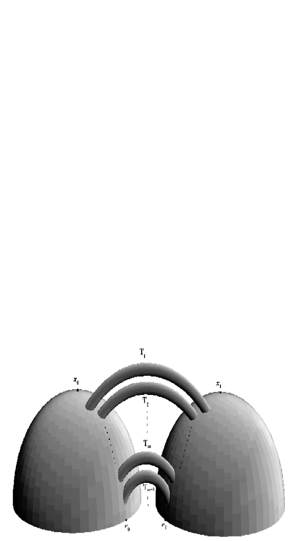
Figure 1: The two hemispheres $H_{0},H_{1}$ are connected by a sequence of inmersed tubes $(T_{m})$ such that the length of a minimizing connecting curve $\gamma_{m}$ through $T_{m}$ is bigger than the length of the corresponding $\gamma_{m+1}$ through $T_{m+1}$.

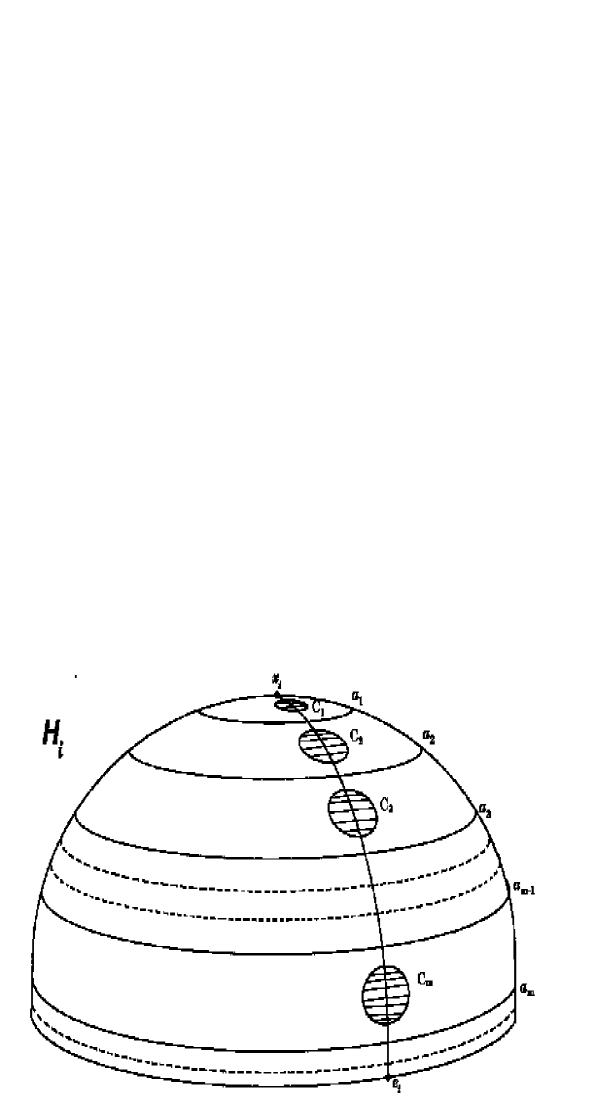
Figure 2: The dashed circles $C_{m}$ are removed to attach the tubes $T_{m}$. The centers of the mouths of the tubes lie in a meridian $\Upsilon$ and converge to an equatorial point $e_{i}$ ($i=0,1$). Each parallel with heigth $a_{m}$ is equal to the connected component of the boundary $\partial{\cal D}_{m}\ \cap H_{i}$, and it is clearly convex.

Consider two open hemispheres $H_{0},H_{1}$ in ${\bf R}^{3}$ and let $x_{0},x_{1}$ be their north poles (see Fig. 1). Put a sequence of inmersed tubes $(T_{m})_{m\in{\bf N}}$ connecting $H_{0}$ and $H_{1}$ of decreasing length and such that any curve joining $x_{0}$ and $x_{1}$ through $T_{m}$ is longer than a minimizing curve joining them through $T_{m+1}$. We also assume that the width of these tubes goes to zero, and their mouths in each hemisphere go to a point $e_{i},i=0,1$ in the equator, being all their centers in the same meridian (the shape of the resulting hemispheres is shown in Fig. 2). Let ${\cal M}$ be this manifold inmersed in ${\bf R}^{3}$, and ${\cal D}={\cal M}$.

Recall that $\partial_{c}{\cal D}$ is canonically identifiable to the equators, and let $\phi:{\cal D}\rightarrow{\bf R}$ be the height function with $\lim_{p\rightarrow\partial_{c}{\cal D}}\phi(p)=0$. Clearly, a sequence $(a_{m})\rightarrow 0$ can be chosen such that $\overline{\cal D}_{m}\ =\phi^{-1}([a_{m},\infty[)$ is a complete Riemannian manifold with convex boundary $\partial{\cal D}_{m}=\phi^{-1}(a_{m})$, containing the tube $T_{m}$ but not $T_{m+1}$, and satisfying (1.8). So, in each convex manifold ${\cal D}_{m}=\phi^{-1}(]a_{m},\infty[)$ there exists a minimizing geodesic $\gamma_{m}$ connecting $x_{0},x_{1}$, and, by the condition on the lengths of the tubes,

$$\hbox{length}\,(\gamma_{m+1})<\hbox{length}\,(\gamma_{m}).$$

So, if there was a minimizing geodesic $\gamma$ between $x_{0},x_{1}$ in ${\cal D}$, necessarily it should be included in some ${\cal D}_{m}$ and $\hbox{length}\,(\gamma_{m+1})<\hbox{length}\,(\gamma)$, a contradiction.

3 Proof of Theorems 1.6 and 1.8

Before introducing the functional framework, we recall that, by the well–known Nash embedding Theorem (see [6]), any smooth Riemannian manifold ${\cal M}$ is isometric to a submanifold of ${\bf R}^{N}$, with $N$ sufficiently large, equipped with the metric induced by the Euclidean metric in ${\bf R}^{N}$. So, henceforth, we shall assume that ${\cal M}$ is a submanifold of ${\bf R}^{N}$ and $\langle\cdot,\cdot\rangle$ is the Euclidean metric. It is well–known that the geodesics in ${\cal D}$ joining two fixed points $p$ and $q$ of ${\cal D}$ are the critical points of the action integral (1.1) defined on $\Omega^{1}\left({\cal D}\right)$ where

$$\Omega^{1}\left({\cal D}\right)=\left\{x\in H^{1,2}([0,1],{\cal D})\mid x(0)=p,x(1)=q\right\}$$

and

$$H^{1,2}([0,1],{\cal D})=\left\{x\in H^{1,2}([0,1],{\bf R}^{N})\mid x([0,1])\subset{\cal D}\right\}.$$

It can be proved that $\Omega^{1}\left({\cal D}\right)$ is a Hilbert submanifold of $H^{1,2}([0,1],{\cal D})$ whose tangent space at $x\in\Omega^{1}\left({\cal D}\right)$ is given by

$$T_{x}\Omega^{1}\left({\cal D}\right)=\left\{v\in H^{1,2}([0,1],T{\cal D})\mid v(s)\in T_{x(s)}{\cal D}\;\;v(0)=0=v(1)\right\}.$$

We recall the following definition.

Definition 3.1

Let $(X,g)$ be a Riemannian manifold modelled on a Hilbert space and let $F\in{\cal C}^{1}(X,{\bf R})$. We say that $F$ satisfies the Palais–Smale condition if every sequence $(x_{m})_{m\in{\bf N}}$ such that

$$(F(x_{m}))_{m\in{\bf N}}\hbox{ is bounded},$$ (3.1)

$$\|\nabla F(x_{m})\|\rightarrow 0,$$ (3.2)

contains a converging subsequence, where $\nabla F(x)$ denotes the gradient of $F$ at the point $x$ with respect to the metric $g$ and $\|\cdot\|$ is the norm on the tangent bundle induced by $g$. A sequence satisfying (3.1)–(3.2) is said a Palais–Smale sequence.

In our case there are Palais–Smale sequences that could converge to a curve which “touches” the boundary $\partial{\cal D}$, so we penalize the functional $f$ in a suitable way, following [1]. For any $\epsilon\in]0,1]$, we consider on $\Omega^{1}\left({\cal D}\right)$ the functional

$$f_{\epsilon}(x)=f(x)+\int_{0}^{1}{\epsilon\over{\phi^{2}(x)}}ds$$ (3.3)

where $\phi$ has been introduced in Theorem 1.6. For any $\epsilon\in]0,1]$ $f_{\epsilon}$ is a ${\cal C}^{2}$ functional and if $x\in\Omega^{1}\left({\cal D}\right)$ is a critical point of $f_{\epsilon}$, by using a boot–strap argument it can be proved that it is ${\cal C}^{2}$ and satisfies

$$D_{s}\dot{x}=-{{2\epsilon}\over{\phi^{3}(x)}}\nabla\phi(x).$$ (3.4)

For any $\epsilon\in]0,1]$, $s\in[0,1]$, we set

$$\lambda_{\epsilon}(s)={{2\epsilon}\over{\phi^{3}(x(s))}},$$ (3.5)

which represents the multiplier in (3.4). Multiplying (3.4) by $\dot{x}$, it is easy to get the existence of a constant $E_{\epsilon}(x)\in{\bf R}$ such that

$${1\over 2}\langle\dot{x}(s),\dot{x}(s)\rangle-{{\epsilon}\over{\phi^{2}(x(s))}}=E_{\epsilon}(x)\quad\forall s\in[0,1].$$ (3.6)

To prove that the penalized functionals satisfy the Palais–Smale condition, we recall the following lemma which holds with slight variants of the proof in [1] also under our local assumptions (i)–(ii) of Theorem 1.6.

Lemma 3.2

Let $(x_{m})_{m\in{\bf N}}$ be a sequence in $\Omega^{1}\left({\cal D}\right)$ such that

$$\sup_{m\in{\bf N}}\int_{0}^{1}\langle\dot{x}_{m},\dot{x}_{m}\rangle ds<\infty$$ (3.7)

and assume the existence of a sequence $(s_{m})_{m\in{\bf N}}$ in $[0,1]$ such that

$$\lim_{m\longrightarrow\infty}\phi(x_{m}(s_{m}))=0.$$ (3.8)

Then

$$\lim_{m\longrightarrow\infty}\int_{0}^{1}{1\over{\phi^{2}(x_{m}(s))}}~{}ds=\infty.$$ (3.9)

Proposition 3.3

Let $f_{\epsilon}$ be as in (3.3). Then

• for any $\epsilon\in]0,1]$ and for any $c\in{\bf R}$ the sublevels

  $$f_{\epsilon}^{c}=\{x\in\Omega^{1}\left({\cal D}\right)|f_{\epsilon}(x)\leq c\}$$

  are complete metric subspaces of $\Omega^{1}\left({\cal D}\right)$;

• for any $\epsilon\in]0,1]$, $f_{\epsilon}$ satisfies the Palais–Smale condition.

Proof: For any $\epsilon\in]0,1],c\in{\bf R}$, let $(x_{m})_{m\in{\bf N}}$ be a Cauchy sequence in $f_{\epsilon}^{c}$, then it is a Cauchy sequence also in $H^{1,2}([0,1],{\bf R}^{N})$, so it converges strongly to a curve $x$ in $H^{1,2}([0,1],{\bf R}^{N})$. Since this convergence is also uniform, by Lemma 3.2 it results that $x\in\Omega^{1}\left({\cal D}\right)$ and by the continuity of $f_{\epsilon}$, we obtain the first part of the proposition. Now let $(x_{m})_{m\in{\bf N}}$ be a Palais–Smale sequence; in particular it results that

$$\int_{0}^{1}\langle\dot{x}_{m},\dot{x}_{m}\rangle ds\quad\hbox{is bounded}.$$ (3.10)

Then, up to a subsequence, we get the existence of a $x\in H^{1,2}([0,1],{\bf R}^{N})$ such that

$$x_{m}\longrightarrow x\hbox{ weakly in }H^{1,2}([0,1],{\bf R}^{N}).$$ (3.11)

Arguing as in the first part of the proof, we get that $x\in\Omega^{1}\left({\cal D}\right)$. Using standard arguments, it can be proved that

$$x_{m}\longrightarrow x\hbox{ strongly in }H^{1,2}([0,1],{\bf R}^{N}).\quad\Box$$

Remark 3.4

By Proposition 3.3, for any $\epsilon\in]0,1]$, $f_{\epsilon}$ has a minimum point $x_{\epsilon}\in\Omega^{1}\left({\cal D}\right)$; it is easy to see that there exists $k>0$ such that

$$f_{\epsilon}(x_{\epsilon})\leq k,$$

for any $\epsilon\in]0,1]$. Moreover, by (3.6) we get for any $\epsilon\in]0,1]$

$$E_{\epsilon}(x_{\epsilon})=f_{\epsilon}(x_{\epsilon})-2\int_{0}^{1}{\epsilon\over{\phi^{2}(x_{\epsilon}(s))}}~{}ds\leq k,$$

hence

$${1\over 2}\langle\dot{x}_{\epsilon}(s),\dot{x}_{\epsilon}(s)\rangle\leq k+{\epsilon\over{\phi^{2}(x_{\epsilon}(s))}},$$ (3.12)

for any $\epsilon\in]0,1]$, $s\in[0,1]$.

Remark 3.5

In the sequel, we shall need to relate the Hessian of a $\hat{\Psi}\in{\cal C}^{2}({\bf R}^{N},{\bf R})$ to the one of its restriction $\Psi$ on ${\cal M}$. For any $y\in{\cal M}$ let

$$P(y):{{\bf R}}^{N}\longrightarrow T_{y}{\cal M},$$ (3.13)

$$Q(y):{\bf R}^{N}\longrightarrow T_{y}{\cal M}^{\perp},$$ (3.14)

be respectively the projections on $T_{y}{\cal M}$ and $T_{y}{\cal M}^{\perp}$. Since ${\cal M}$ is a ${\cal C}^{3}$ submanifold of ${\bf R}^{N}$, there exist $A^{i}_{j}\in{\cal C}^{2}({\cal M},{\bf R})$, $i$,$j\in\{1,\dots,N\}$ such that for any $y\in{\cal M},v=(v^{1},\ldots,v^{N})\in{\bf R}^{N}$

$$Q(y)[v]=\sum_{i,j=1}^{N}A^{i}_{j}(y)v^{j}e_{i},$$

where $e_{1},...,e_{N}$ is the canonical basis of ${\bf R}^{N}$. We locally extend the functions $A^{i}_{j}$ to ${\cal C}^{2}$ functions (still denoted by $A^{i}_{j}$) on ${\bf R}^{N}$. For any $y\in{\bf R}^{N}$, we define the differential map ${\rm d}Q(y)\colon{\bf R}^{N}\times{\bf R}^{N}\longrightarrow{\bf R}^{N}$ as

$${\rm d}Q(y)[v,w]=\sum_{i,j,k=1}^{N}{{\partial A_{j}^{i}(y)}\over\partial{x_{k}}}v^{k}w^{j}e_{i},\quad\forall v,w\in{\bf R}^{N}.$$

Even if ${\rm d}Q$ could depend on the extensions of the functions $A^{i}_{j}$, for any $y\in{\cal M}$, the restriction of ${\rm d}Q(y)$ to $T_{y}{\cal M}\times T_{y}{\cal M}$ is well–defined. It can be proved (see e.g. [3, Lemma 8]) that for any $y\in{\cal M}$, $v\in T_{y}{\cal M}$:

$$H_{\Psi}(y)[v,v]={\rm d}^{2}\hat{\Psi}(y)[v,v]-{\rm d}\hat{\Psi}(y)[{\rm d}Q(y)[v,v]],$$

where $d$ and $d^{2}$ are the differential map and the second differential map on ${\bf R}^{N}$.

Lemma 3.6

Let $\left(x_{\epsilon}\right)_{\epsilon>0}$ be a family in $\Omega^{1}({\cal D})$ of critical points of $f_{\epsilon}$ such that

$$f_{\epsilon}(x_{\epsilon})\leq k\quad\forall\epsilon\in]0,1],$$ (3.15)

for a suitable positive constant $k$. Then ${\displaystyle\left(\lambda_{\epsilon}(s)={{2\epsilon}\over{\phi^{3}(x_{\epsilon}(s))}}\right)_{\epsilon>0}}$ is bounded in $L^{\infty}\left([0,1],{\bf R}\right)$.

Proof: Let $\left(\epsilon_{m}\right)_{m\in{\bf N}}$ be a decreasing and infinitesimal sequence in $]0,1]$ and let $\left(x_{\epsilon_{m}}\right)_{m\in{\bf N}}$ be a sequence of critical points of $f_{\epsilon_{m}}$ satisfying (3.15). For the sake of simplicity, in the following we set $x_{\epsilon_{m}}\equiv x_{m}$, $\lambda_{\epsilon_{m}}\equiv\lambda_{m}$. Now let $u_{m}(s)=\phi(x_{m}(s))$, for $s\in[0,1],m\in{\bf N}$ and $u_{m}(s_{m})=\min_{s\in[0,1]}u_{m}(s)$, for any $m\in{\bf N}$. It suffices to prove the lemma when, up to a subsequence,

$$\lim_{m\longrightarrow\infty}u_{m}(s_{m})=0.$$ (3.16)

By (3.15) and the Poincaré inequality there exists $x\in H^{1,2}([0,1],{\bf R}^{N})$ such that

$$x_{m}\longrightarrow x\quad\hbox{uniformly},$$ (3.17)

and since, up to a subsequence,

$$\lim_{m\longrightarrow\infty}s_{m}=s_{0},$$ (3.18)

by (3.16) and (3.17) it easily follows $s_{0}\in]0,1[$ since $\phi(p),\phi(q)>0$. It is not difficult to see that $\left(x_{m}(s_{m})\right)_{m\in{\bf N}}$ converges to $x(s_{0})=y\in\partial{\cal D}$. Let $U$ be a neighborhood of $y$ such that (ii)–(iv) of Theorem 1.6 hold, then there exists $\mu>0$ such that

$$x_{m}(s)\in U\cap{\cal D}$$ (3.19)

for any $s\in J=[s_{0}-\mu,s_{0}+\mu]$ and $m$ sufficiently large. By (3.4), (3.5), (3.16) and (ii) of Theorem 1.6, we get for m large enough

$$\ddot{u}_{m}(s_{m})=H_{\phi}(x_{m}(s_{m}))[\dot{x}_{m}(s_{m}),\dot{x}_{m}(s_{m})]-\lambda_{m}(s_{m}){\|\nabla\phi(x_{m}(s_{m}))\|}^{2}\leq$$

$$H_{\phi}(x_{m}(s_{m}))[\dot{x}_{m}(s_{m}),\dot{x}_{m}(s_{m})]-a^{2}\lambda_{m}(s_{m}).$$ (3.20)

By the assumptions of Theorem 1.6 and (3.16), for any $m\in{\bf N}$ there exists $k_{m}\in{\bf N}$ such that

$$a_{k_{m}}\leq\phi(x_{m}(s_{m}))\leq\phi(x_{m}(s))$$

for any $s\in[0,1]$. Let us consider the Cauchy problem

$$\left\{\begin{array}[]{ll}{\displaystyle\dot{\eta}=-\frac{\nabla\phi(\eta)}{\|\nabla\phi(\eta)\|^{2}}}\\ \eta(0)=x\in U\cap{\cal D}\end{array}\right.$$ (3.21)

and call $\eta(s,x):{\cal U}\subset{\bf R}\times\overline{\cal D}\longrightarrow\overline{\cal D}$ the flow associated to the Cauchy problem (3.21), where ${\cal U}$ is the maximal domain where the flow can be defined. Set for any $s\in J$

$$\tau_{m}(s)=\phi(x_{m}(s))-a_{k_{m}}$$ (3.22)

$$y_{m}(s)=\eta\left(\tau_{m}(s),x_{m}(s)\right).$$ (3.23)

Observe that if $m$ is sufficiently large and $\mu$ is opportunely chosen

$$(\tau_{m}(s),x_{m}(s))\in{\cal U}\qquad y_{m}(s)\in U\qquad\forall s\in J.$$

Then, for $m$ large enough, we can define the projection $\Pi_{m}:U\cap{\cal D}\longrightarrow\phi^{-1}(a_{k_{m}})$

$$\Pi_{m}(x_{m}(s))=y_{m}(s)\quad s\in J.$$ (3.24)

Note that, by the definition of $\Pi_{m}$, $\langle\dot{y}_{m}(s),\nabla\phi(y_{m}(s))\rangle=0$, for any $s\in J$, so since

$$\dot{y}_{m}(s)=\eta_{x}\left(\tau_{m}(s),x_{m}(s)\right)[\dot{x}_{m}(s)]-{{\nabla\phi(y_{m}(s))}\over{{\|\nabla\phi(y_{m}(s))\|}^{2}}}\dot{u}_{m}(s),$$

by assumption (iii) of Theorem 1.6 we get for any $s\in J$

$${\displaystyle{|\dot{y}_{m}(s)|}^{2}={|\eta_{x}\left(\tau_{m}(s),x_{m}(s)\right)[\dot{x}_{m}(s)]|}^{2}-{{\dot{u}_{m}^{2}(s)}\over{{\|\nabla\phi(y_{m}(s))\|}^{2}}}\leq}$$

$${\displaystyle C|\dot{x}_{m}(s)|^{2}.}$$ (3.25)

Hence by (3) and (iv) of Theorem 1.6

$${\displaystyle a^{2}\lambda_{m}(s_{m})\leq H_{\phi}(x_{m}(s_{m}))[\dot{x}_{m}(s_{m}),\dot{x}_{m}(s_{m})]-H_{\phi}(y_{m}(s_{m}))[\dot{y}_{m}(s_{m})),\dot{y}_{m}(s_{m})]+}$$

$${\displaystyle M\langle\dot{y}_{m}(s_{m}),\dot{y}_{m}(s_{m})\rangle a_{k_{m}}.}$$ (3.26)

Now, following Remark 3.5, set for any $x\in{\cal D}$, $v,w\in{\bf R}^{N}$

$$L(x)[v,w]={\rm d}^{2}\phi(x)[v,w]-{\rm d}\phi(x)[{\rm d}Q(x)[v,w]],$$ (3.27)

$${\displaystyle H_{\phi}(x_{m}(s_{m}))[\dot{x}_{m}(s_{m}),\dot{x}_{m}(s_{m})]-H_{\phi}(y_{m}(s_{m}))[\dot{y}_{m}(s_{m}),\dot{y}_{m}(s_{m})]=}$$

$${\displaystyle L(x_{m}(s_{m}))[\dot{x}_{m}(s_{m}),\dot{x}_{m}(s_{m})]-L(y_{m}(s_{m}))[\dot{y}_{m}(s_{m}),\dot{y}_{m}(s_{m})]=}$$

$${\displaystyle L(x_{m}(s_{m}))[\dot{x}_{m}(s_{m}),\dot{x}_{m}(s_{m})]-L(y_{m}(s_{m}))[\dot{x}_{m}(s_{m}),\dot{x}_{m}(s_{m})]+}$$

$${\displaystyle L(y_{m}(s_{m}))[\dot{x}_{m}(s_{m}),\dot{x}_{m}(s_{m})]-L(y_{m}(s_{m}))[\dot{y}_{m}(s_{m}),\dot{y}_{m}(s_{m})]=}$$

$${\displaystyle L(x_{m}(s_{m}))[\dot{x}_{m}(s_{m}),\dot{x}_{m}(s_{m})]-L(y_{m}(s_{m}))[\dot{x}_{m}(s_{m}),\dot{x}_{m}(s_{m})]+}$$

$${\displaystyle L(y_{m}(s_{m}))[\dot{x}_{m}(s_{m})+\dot{y}_{m}(s_{m}),\dot{x}_{m}(s_{m})-\dot{y}_{m}(s_{m})].}$$ (3.28)

In the following we shall denote by $M_{1},\ldots,M_{7}$ suitable positive constants. Since $\phi\in{\cal C}^{3}$, $\eta\in{\cal C}^{2}$, using the mean value theorem, the boundness of $\left(\|x_{m}\|_{\infty}\right)_{m\in{\bf N}}$ and $\left(\|y_{m}\|_{\infty}\right)_{m\in{\bf N}}$, (iii) of Theorem 1.6 and (3.16):

$${\displaystyle L(x_{m}(s_{m}))[\dot{x}_{m}(s_{m}),\dot{x}_{m}(s_{m})]-L(y_{m}(s_{m}))[\dot{x}_{m}(s_{m}),\dot{x}_{m}(s_{m})]\leq}$$

$${\displaystyle M_{1}{|\dot{x}_{m}(s_{m})|}^{2}|x_{m}(s_{m})-y_{m}(s_{m})|\leq}$$

$${\displaystyle M_{2}{|\dot{x}_{m}(s_{m})|}^{2}\left(u_{m}(s_{m})-a_{k_{m}}\right)\leq}$$

$${\displaystyle M_{3}{|\dot{x}_{m}(s_{m})|}^{2}.}$$ (3.29)

By the boundness of $\left(\|y_{m}\|_{\infty}\right)_{m\in{\bf N}}$ and (3) we get

$${\displaystyle L(y_{m}(s_{m}))[\dot{x}_{m}(s_{m})+\dot{y}_{m}(s_{m}),\dot{x}_{m}(s_{m})-\dot{y}_{m}(s_{m})]\leq}$$

$${\displaystyle M_{4}{|\dot{x}_{m}(s_{m})|}^{2}}.$$ (3.30)

Then by (3), (3), (3), (3), (3), we get

$$a^{2}\lambda_{m}(s_{m})\leq M_{5}{|\dot{x}_{m}(s_{m})|}^{2}$$

so that (3.12) implies

$${\epsilon_{m}\over{\phi^{3}(x_{m}(s_{m}))}}\leq M_{6}+M_{7}{\epsilon_{m}\over{\phi^{2}(x_{m}(s_{m}))}}$$

from which the boundedness of the multiplier follows. $\Box$

Proposition 3.7

Let $\left(x_{\epsilon}\right)_{\epsilon>0}$ be a sequence of critical points of $f_{\epsilon}$ and $k$ a positive constant such that (3.15) holds. Then there exists a positive constant $\beta$ such that

$$\phi(x_{\epsilon}(s))\geq\beta\quad\forall s\in[0,1],\epsilon\in]0,1].$$ (3.31)

Proof: Assume by contradiction that there exist a decreasing and infinitesimal sequence $\left(\epsilon_{m}\right)_{m\in{\bf N}}\in]0,1]$ and a sequence $\left(x_{\epsilon_{m}}\right)_{m\in{\bf N}}$ of critical points of $f_{\epsilon_{m}}$ satisfying (3.15) and such that

$$\min_{s\in[0,1]}\phi(x_{\epsilon_{m}}(s))\rightarrow 0\hbox{ as }m\longrightarrow\infty.$$ (3.32)

Defining $x_{m},u_{m},s_{m},s_{0},U,J$ and $a_{k_{m}}$ as in Lemma 3.6, since for $s\in J$, $m\in{\bf N}$ sufficiently large $y_{m}(s)\in U$, we get, by (iv) of Theorem 1.6

$${\displaystyle\ddot{u}_{m}(s)\leq H_{\phi}(x_{m}(s))[\dot{x}_{m}(s),\dot{x}_{m}(s)]-H_{\phi}(y_{m}(s))[\dot{y}_{m}(s),\dot{y}_{m}(s)]+}$$

$${\displaystyle M\phi(y_{m}(s))\langle\dot{y}_{m}(s),\dot{y}_{m}(s)\rangle-{{2\epsilon_{m}}\over{\phi^{3}(x_{m}(s))}}{\|\nabla\phi(x_{m}(s))\|}^{2}\leq}$$

$${\displaystyle H_{\phi}(x_{m}(s))[\dot{x}_{m}(s),\dot{x}_{m}(s)]-H_{\phi}(y_{m}(s))[\dot{y}_{m}(s),\dot{y}_{m}(s)]+}$$

$${\displaystyle M\phi(y_{m}(s))\langle\dot{y}_{m}(s),\dot{y}_{m}(s)\rangle}$$ (3.33)

where $y_{m}$ is defined by (3.22) and (3.23). In the following we shall always assume $s\in J$ and $m\in{\bf N}$ large enough and we shall denote by $C_{1},\ldots,C_{11}$ suitable positive constants. Now by (3.27)

$${\displaystyle H_{\phi}(x_{m}(s))[\dot{x}_{m}(s),\dot{x}_{m}(s)]-H_{\phi}(y_{m}(s))[\dot{y}_{m}(s),\dot{y}_{m}(s)]=}$$

$${\displaystyle L(x_{m}(s))[\dot{x}_{m}(s),\dot{x}_{m}(s)]-L(y_{m}(s))[\dot{y}_{m}(s),\dot{y}_{m}(s)]=}$$

$${\displaystyle L(x_{m}(s))[\dot{x}_{m}(s),\dot{x}_{m}(s)]-L(y_{m}(s))[\dot{x}_{m}(s),\dot{x}_{m}(s)]+}$$

$${\displaystyle L(y_{m}(s))[\dot{x}_{m}(s)+\dot{y}_{m}(s),\dot{x}_{m}(s)-\dot{y}_{m}(s)].}$$ (3.34)

Since $\phi\in{\cal C}^{3}$, $\eta\in{\cal C}^{2}$, using the mean value theorem, the boundness of $\left(\|x_{m}\|_{\infty}\right)_{m\in{\bf N}}$ and $\left(\|y_{m}\|_{\infty}\right)_{m\in{\bf N}}$ and (iii) of Theorem 1.6, there results

$${\displaystyle L(x_{m}(s))[\dot{x}_{m}(s),\dot{x}_{m}(s)]-L(y_{m}(s))[\dot{x}_{m}(s),\dot{x}_{m}(s)]\leq}$$

$${\displaystyle C_{1}{|\dot{x}_{m}(s)|}^{2}u_{m}(s).}$$ (3.35)

Since $\eta_{x}(0,x)[v]=v$,

$${\displaystyle\dot{x}_{m}(s)-\dot{y}_{m}(s)=\eta_{x}(0,x_{m}(s))[\dot{x}_{m}(s)]-}$$ (3.36)

$${\displaystyle\eta_{x}(\tau_{m}(s),x_{m}(s))[\dot{x}_{m}(s)]-\eta_{s}(\tau_{m}(s),x_{m}(s))\dot{u}_{m}(s),}$$

so by (3.36) the mean value theorem and (iii) of Theorem 1.6

$${\displaystyle L(y_{m}(s))[\dot{x}_{m}(s)+\dot{y}_{m}(s),\dot{x}_{m}(s)-\dot{y}_{m}(s)]=}$$

$${\displaystyle L(y_{m}(s))[\dot{x}_{m}(s)+\dot{y}_{m}(s),\eta_{x}(0,x_{m}(s))[\dot{x}_{m}(s)]-\eta_{x}(\tau_{m}(s),x_{m}(s))[\dot{x}_{m}(s)]]-}$$

$${\displaystyle L(y_{m}(s))[\dot{x}_{m}(s)+\dot{y}_{m}(s),\eta_{s}(\tau_{m}(s),x_{m}(s))\dot{u}_{m}(s)]\leq}$$

$${\displaystyle C_{2}{|\dot{x}_{m}(s)|}^{2}u_{m}(s)+B_{m}(s)\dot{u}_{m}(s)}$$ (3.37)

where

$$B_{m}(s)=-L(y_{m}(s))[\dot{x}_{m}(s)+\dot{y}_{m}(s),\eta_{s}(\tau_{m}(s),x_{m}(s))]$$ (3.38)

is a ${\cal C}^{1}$ function. By (3.12), (3.19), Lemma 3.6 and (ii) of Theorem 1.6 we get

$$\langle\dot{x}_{m}(s),\dot{x}_{m}(s)\rangle\leq C_{3}$$ (3.39)

for a suitable constant $C_{3}$, hence by (3), (3), (3) and (3) we get

$$\ddot{u}_{m}(s)\leq C_{4}u_{m}(s)+B_{m}(s)\dot{u}_{m}(s).$$ (3.40)

Note that by (3.39) and (iii) of Theorem 1.6

$$|B_{m}(s)|\leq C_{5}$$ (3.41)

and by (3.4), (ii) of Theorem 1.6

$$|D_{s}\dot{x}_{m}(s)|\leq C_{6}.$$

Since

$$\ddot{x}_{m}(s)=P(x_{m}(s))\ddot{x}_{m}(s)+Q(x_{m}(s))\ddot{x}_{m}(s)$$

$$=D_{s}\dot{x}_{m}(s)-dQ(x_{m}(s))[\dot{x}_{m}(s),\dot{x}_{m}(s)]$$

where $P,Q$ are as in (3.13), (3.14), we also get

$$|\ddot{x}_{m}|\leq C_{7}.$$

Then by using (iii) of Theorem 1.6, standard arguments show that

$$|\dot{B}_{m}(s)|\leq C_{8}.$$ (3.42)

Therefore by (3.40), (3.41) and (3.42) integrating by parts, for $s>s_{m}$ there results

$${\displaystyle\dot{u}_{m}(s)=\int_{s_{m}}^{s}\ddot{u}_{m}(\tau)d\tau\leq C_{4}\int_{s_{m}}^{s}u_{m}(\tau)d\tau+\int_{s_{m}}^{s}B_{m}(\tau)\dot{u}_{m}(\tau)d\tau=}$$

$${\displaystyle C_{4}\int_{s_{m}}^{s}u_{m}(\tau)d\tau+B_{m}(s)u_{m}(s)-B_{m}(s_{m})u_{m}(s_{m})-\int_{s_{m}}^{s}\dot{B}_{m}(\tau)u_{m}(\tau)d\tau\leq}$$

$${\displaystyle C_{9}\int_{s_{m}}^{s}u_{m}(\tau)d\tau+C_{5}u_{m}(s)+C_{5}u_{m}(s_{m}).}$$ (3.43)

Hence

$${\displaystyle u_{m}(s)\leq u_{m}(s_{m})+C_{9}\int_{s_{m}}^{s}\left(\int_{s_{m}}^{\tau}u_{m}(r)dr\right)d\tau+C_{5}\int_{s_{m}}^{s}u_{m}(\tau)d\tau+C_{5}u_{m}(s_{m})\leq}$$

$${\displaystyle C_{10}u_{m}(s_{m})+C_{11}\int_{s_{m}}^{s}u_{m}(\tau)d\tau.}$$ (3.44)

By the Gronwall lemma we get

$$u_{m}(s)\leq C_{10}u_{m}(s_{m})\exp(C_{11}(s-s_{m}))$$

so by (3.32) we have

$$u_{m}\longrightarrow 0\hbox{ uniformly}$$

getting a contradiction. $\Box$

Proof of Theorem 1.6. By Remark 3.4 and Proposition 3.7, we can find a family $\left(x_{\epsilon}\right)_{\epsilon>0}$ of critical points of $f_{\epsilon}$ such that (3.31) holds. By (3.15) and the Poincaré inequality, $\left(x_{\epsilon}\right)_{\epsilon>0}$ is bounded in $H^{1,2}([0,1],{\bf R}^{N})$, so there is a subsequence $\left(x_{\epsilon_{m}}\right)_{m\in{\bf N}}$ such that

$$x_{\epsilon_{m}}\longrightarrow x\hbox{ weakly in }\,H^{1,2}([0,1],{\bf R}^{N}),$$ (3.45)

where $x\in\Omega^{1}\left({\cal D}\right)$ since the convergence is also uniform and (3.31) holds. Now it is easy to prove that $f$ attains a minimum value at $x$. Indeed by (3.45) and (3.3)

$$f(x)\leq\liminf_{m\longrightarrow\infty}f_{\epsilon_{m}}(x_{\epsilon_{m}})\leq f(y)$$

for any $y\in\Omega^{1}\left({\cal D}\right)$, so ${\cal D}$ is convex. Finally, if ${\cal D}$ is not contractible in itself, the proof can be carried out exactly as the one of Theorem 0.2 of [8]. $\Box$

Proof of Theorem 1.8. The only difference with the proof of Theorem 1.6 concerns the a priori estimates of Proposition 3.7 that here are simpler because they do not require a projection. Indeed, defining $x_{m}$, $u_{m}$, $s_{m}$, $J$ as in Proposition 3.7, we get by (ii) and (iii) of Theorem 1.8, for $m$ sufficiently large

$$\ddot{u}_{m}(s)\leq M\phi(x_{m}(s))\langle\dot{x}_{m}(s),\dot{x}_{m}(s)\rangle-\frac{2\epsilon_{m}a^{2}}{\phi^{3}(x_{m}(s))}.$$

As (3.12) holds, we get

$$\ddot{u}_{m}(s)\leq M_{1}u_{m}(s)+M_{2}\frac{\epsilon_{m}}{u_{m}(s)}-M_{3}\frac{\epsilon_{m}}{u_{m}^{3}(s)}$$

for $M_{1},M_{2},M_{3}>0$, so that, if $\delta$ is sufficiently small

$$\ddot{u}_{m}(s)\leq M_{1}u_{m}(s).$$

Then, by the Gronwall Lemma, we immediately get a contradiction. $\Box$

4 Applications

(a) Some examples. (1) First, we will check that Theorems 1.6, and 1.8 can be applied in cases where neither the elementary considerations for differentiable boundary nor Theorem 1.5 are appliable. Let $({\cal M},\langle\cdot,\cdot\rangle)$ be a cylinder $C$ in ${\bf R}^{3}$ and let $H$ be an helix in $C$. Set ${\cal D}=C\setminus H$ and take $\phi$ equal to the distance to $H$ on a strip $S$ around $H$. Recall that ${\cal D}$ cannot be considered as a manifold with boundary $\partial{\cal D}=H.$ Clearly, Theorems 1.6 and 1.8 are applicable and, moreover, we can perturb the metric to make the constant $M$ in (1.9) positive (for example, by conformally changing the metric symmetrically around $H$ on $S$, see formula (4.3)); thus, Theorem 1.5 may be not applicable now.

(2) Nevertheless, the following example shows that Theorem 1.5 may be applicable when Theorems 1.6, 1.8 are not, even if the condition for the Hessian in Theorem 1.8 is satisfied. Consider ${\cal D}=]0,\infty[\times]0,\infty[$, and ${\cal M}={\bf R}^{2}$ equipped with the Euclidean metric (this metric can be perturbed as suggested in last example to make this one non–trivial; note that conditions (ii), (iii) in Theorem 1.6 are independent of the metric on ${\cal M}$). If $\phi(x,y)=\sqrt{xy}$, then

$${\|\nabla\phi(x,y)\|}^{2}={{x^{2}+y^{2}}\over{4xy}}>{1\over 4},$$

so the first inequality in (ii) of Theorems 1.6, 1.8 is satisfied, but not the second one. On the other hand, if we choose $\hat{\phi}(x,y)=xy$ then

$${\|\nabla\hat{\phi}(x,y)\|}^{2}=x^{2}+y^{2},$$

which satisfies the upper local bound around each point, but not the lower one (compare with Remark 1.7(2)). Nevertheless, it is straightforward to check that Theorem 1.5 is applicable for $\phi$ as well as for $\hat{\phi}$.

(3) It is clear that condition (iii) of Theorem 1.8 on all tangent vectors $v$ may not hold under the corresponding hypothesis (iv) of Theorem 1.6. The following example shows that Theorem 1.8 may be appliable when Theorem 1.6 is not, because of the hypothesis (iii) of this theorem and the requirement that ${\cal D}$ must be a subset of a complete manifold. Consider ${\cal D}={\cal M}={\bf R}\setminus\{0\}\times{\bf R}$ endowed with the Riemannian metric given in polar coordinates $r,\theta$ by

$$dx^{2}=dr^{2}+{1\over{r^{2}}}d\theta^{2}.$$

Choosen $\phi(r,\theta)=r$, it follows $\nabla\phi=\partial_{r}$, so $\|\nabla\phi(r,\theta)\|=1$. Standard calculations show that the (normalized) flow of $\nabla\phi$ is $\eta(s,(r,\theta))=(r-s,\theta)$ and the norm of the partial derivative $\eta_{(r,\theta)}$ is not bounded, so we cannot apply Theorem 1.6. Moreover, note that ${\cal M}$ is not complete and its curvature along incomplete radial geodesics diverges, so ${\cal D}$ is not isometric to a domain of a complete Riemannian manifold ($\partial_{c}{\cal D}$ is topologically a circumference). However, it is easy to check that Theorem 1.8 is applicable.

(b) Trajectories of Lagrangian systems. The interest in the study of the geodesic connectedness of a complete Riemannian manifold is related to the existence of trajectories of a Lagrangian system joining two fixed points. More precisely, consider a potential $V\in C^{2}({\cal M},{\bf R})$ bounded from above in a domain ${\cal D}$ and the system

$$\left\{\begin{array}[]{ll}D_{s}\dot{x}=-\nabla V(x)\\ x(0)=p,x(1)=q.\end{array}\right.$$ (4.1)

Each solution $x:[0,1]\rightarrow{\cal D}$ of (4.1) has constant energy, that is, there exists $E\in{\bf R}$ such that, for any $s\in[0,1]$

$$\frac{1}{2}\langle\dot{x},\dot{x}\rangle+V(x)=E.$$

We fix $E>\sup_{\cal D}V$ and consider the Jacobi metric

$$\langle\cdot,\cdot\rangle_{E}=(E-V(x))\langle\cdot,\cdot\rangle\quad\quad\hbox{on }\overline{\cal D}.$$ (4.2)

As $\overline{\cal D}$ is complete for $\langle\cdot,\cdot\rangle$ then it is also complete for $\langle\cdot,\cdot\rangle_{E}$ and, thus, we can extend $\langle\cdot,\cdot\rangle_{E}$ to a complete Riemannian metric on all ${\cal M}$. It is well–known that the geodesics on ${\cal D}$ with respect to the Riemannian metric $\langle\cdot,\cdot\rangle_{E}$ are, up to reparametrizations, solutions of (4.1) with energy $E$ and vice–versa. Let $\phi$ be a function satisfying conditions (i), (ii), (iii) in Theorem 1.6, which are independent of the metric. If assumption (iv) is satisfied with respect to $\langle\cdot,\cdot\rangle_{E}$ then the existence of at least one solution of (4.1) with energy $E$ is proved. Notice that the Hessian of $\phi$ with respect the two metrics is linked by the following relation

$$H^{E}_{\phi}(x)[v,v]=H_{\phi}(x)[v,v]+\langle\nabla\phi(x),\nabla u(x)\rangle\langle v,v\rangle-2\langle\nabla u(x),v\rangle\langle\nabla\phi(x),v\rangle$$ (4.3)

for any $x\in{\cal M}$, $v\in T_{x}{\cal M}$ where

$$u(x)=\frac{1}{2}\log(E-V(x)).$$

Thus, if (iv) of Theorem 1.6 is verified with respect to $\langle\cdot,\cdot\rangle$, then it is satisfied by $\langle\cdot,\cdot\rangle_{E}$ when for each $y\in\partial{\cal D}$ there exists a neighborhood $U$ and a (positive) constant $M^{\prime}\in{\bf R}$ such that

$$\langle\nabla\phi(x),\nabla V(x)\rangle\geq-M^{\prime}\phi(x)$$ (4.4)

$\forall x\in\phi^{-1}(a_{m})\cap U$. Summing up the following result holds.

Corollary 4.1

Let $\left({\cal M},\langle\cdot,\cdot\rangle\right)$ be a complete Riemannian manifold and assume that there exists a positive and differentiable function $\phi$ on ${\cal D}$ satisfying (i)–(iv) of Theorem 1.6. Then, if $V\in C^{2}({\cal M},{\bf R})$ is bounded from above on ${\cal D}$ and (4.4) holds, for any $E>\sup_{\cal D}V$ there exists a solution with energy $E$ of (4.1). Moreover, if ${\cal D}$ is non contractible in itself, then for any $E>\sup V$ there exist infinitely many solutions of (4.1) with energy $E$.

Acknowledgment. We wish to thank Domingo Rodríguez for his kind help for the figures of this paper.

References

• [1] V. Benci, D. Fortunato, F. Giannoni, On the existence of geodesics in static Lorentz manifolds with singular boundary, Ann. Sc. Normale Sup. Pisa Serie IV XIX, 255-289, (1992).
• [2] R.L. Bishop, Infinitesimal convexity implies local convexity, Indiana Math. J. 24 No. 2, 169-172, (1974).
• [3] A. Germinario, Homoclinics on Riemannian manifolds with convex boundary, Dynam. Systems and Appl., 4, 549-566, (1995).
• [4] W.B. Gordon, The existence of geodesics joining two given points J. Diff. Geom. 9, 443-450, (1974).
• [5] A. Masiello, Variational Methods in Lorentzian Geometry. Pitman Res. Notes in Math. 309: London, 1994.
• [6] J. Nash, The embedding problem for Riemannian manifolds, Ann. of Math. 63, 20-63, (1956).
• [7] K.Nomizu, H.Ozeki, The existence of complete Riemannian metrics, Proc. Amer. Math. Soc. 12, 889-891, (1961).
• [8] A. Salvatore, A two points boundary value problem on non complete Riemannian manifolds, Variational Methods in Nonlinear Analysis, A. Ambrosetti, K.C. Chang editors, Gordon and Breach Publishers, 149-160, (1995).
Refer to caption