Model Sets: A Survey

Abstract

This article surveys the mathematics of the cut and project method as applied to point sets, called here model sets. It covers the geometric, arithmetic, and analytical sides of this theory as well as diffraction and the connection with dynamical systems.

Dedicated to the memory of Richard (Dick) Slansky

The spirit of the universe is subtle and informs all life. Things live and die and change their forms, without knowing the root from which they come. Abundantly it multiplies; eternally it stands by itself. The greatest reaches of space do not leave its confines, and the smallest down of a bird in autumn awaits its power to assume form. — Chuang Tzu (tr. Lin Yutang)

1 Introduction

Even when reduced to its simplest form, namely that of point sets in euclidean space, the phenomenon of genuine quasi-periodicity appears extraordinary. Although it seems unfruitful to try and define the concept precisely, the following properties may be considered as representative:

• discreteness

• extensiveness

• finiteness of local complexity

• repetitivity

• diffractivity

• aperiodicity

• existence of exotic symmetry (optional).

The purpose of this paper is to give an overview of the mathematics of the cut and project method which not only provides a very rich harvest of point sets (called model sets) satisfying these properties, but also provides a very natural way to link these ideas with many other structures in mathematics.

A subset $\Lambda$ of $\mathbb{R}^{d}$ is called a Delone (Delaunay) set if it is uniformly discrete and relatively dense. This means that there are radii $r,R>0$ so that each ball of radius $r$ (resp. $R$) contains at most (resp. at least) one point of $\Lambda$. Although this is a fairly strong version of the first two items on our list, it is the most commonly used one and coincides well with the primitive atomic picture of a (ideally infinite) piece of material.

The set $\Lambda$ has finite local complexity if for each $r>0$ there are, up to translation, only finitely many point sets (called patches of radius $r$) of the form $\Lambda\cap B_{r}(v)$. Here $B_{r}(v)$ is the ball of radius $r$ about the point $v\in\mathbb{R}^{d}$. So, on each scale, there are only finitely many different patterns of points. This condition can be expressed topologically: $\Lambda$ has finite local complexity iff the closure of $\Lambda-\Lambda$ is discrete. It is conceivable to replace “translation” by “isometry” in this definition, but the theory would change considerably and, with the notable exception of the pinwheel tiling [31], little has been said so far on this more general situation.

Repetitivity means loosely that any finite patch that appears, appears infinitely often. More precisely, given any patch of radius $r$ there is an $R$ so that within each ball of radius $R$, no matter its position in $\mathbb{R}^{d}$, there is at least one translate of this patch. A stronger form of this requires in addition that each type of patch of radius $r$ should appear with a well-defined frequency. The sets that we deal with here normally have this additional property (see Section 3).

From the very beginning, diffractivity has been the hallmark of aperiodic order. Physically it is the most visible of its manifestations. Mathematically it is one of the most subtle and least visible! Very roughly we are asking (mathematically) that the Fourier transform of the autocorrelation density that arises by placing a delta peak on each point of $\Lambda$, should contain a part that looks discrete and point-like. Later on we will make this very vague prescription precise. The amazing thing is that in the context of model sets we obtain perfect diffractiveness, in the sense that the diffraction is purely point-like, under the fairly mild hypothesis of regularity. One of the goals of this survey is to show how this comes about.

Lack of periodicity speaks for itself. Lattices and unions of cosets of lattices are the basis of the most prevalent forms of long-range order (crystallography). Point sets based on them satisfy all the previous properites. But of course, that is the trivial part of the theory! The objective is to move into new territory.

Exotic symmetry usually means non-crystallographic symmetry. Although not mathematically essential, certainly the existence of physical structures with “forbidden” icosahedral symmetry was instrumental in the rapid development of this field.

Even with the rather strong interpretations on the various properties listed above, we still do not know how to characterize sets that satisfy them. For an extensive discussion of these problems see [24]. However there is one very general method of construction which relies on controlled projection from a discrete group located in some auxilliary “embedding” space. In its original form this so-called cut and project method is based on projection from lattices in higher dimensional spaces. Many people have written about this starting, in physics, with the work of P. Kramer [21] and including the very useful article of Y. Meyer given in the previous edition of this School [26]. Meyer had already thought about sets formed by projection from the view point of harmonic analysis long before the discovery of quasi-crystals [25]. Even though it is convenient to somewhat rearrange the main components of his original construction, nonetheless he created a formalism which is ideal for creation of points sets with the desired properties of long-range aperiodic order. These are the model sets.

Some people object to the terminolgy “model set” prefering “cut and project set” which sounds more serious and professional. However, we prefer to interpret “model” as meaning exemplary and think that in terms of both of its priority and its greater generality the term deserves to be adopted.

The main purpose of this article is first to give some idea of the scope of the relevant examples that arise as model sets (this scope surely not yet fully realized) and then to show how the model sets are poised between a number of quite different areas of mathematics. It is the satisfying way in which they connect many diverse parts of mathematics that makes model sets so intriguing and offers to the imagination so many tantalizing prospects for future work. For the reader interested in more on the tiling side of quasiperiodicity we recommend the survey paper [1], which also provides a complementary source of some of the material presented here.

2 Model sets

Let us launch ourselves directly into the notion of a model set. By definition, a cut and project scheme consists of a collection of spaces and mappings

$$\begin{array}[]{ccccc}\mathbb{R}^{d}&\stackrel{{\scriptstyle\pi_{1}}}{{\longleftarrow}}&\mathbb{R}^{d}\times G&\stackrel{{\scriptstyle\pi_{2}}}{{\longrightarrow}}&G\\ &&\cup&&\\ &&{\tilde{L}}&&\end{array}$$ (1)

where $\mathbb{R}^{d}$ is a real euclidean space and $G$ is some locally compact abelian group, $\pi_{1}$ and $\pi_{2}$ are the projection maps onto them, and ${\tilde{L}}\subset\mathbb{R}^{d}\times G$ is a lattice, i.e., a discrete subgroup such that the quotient group $(\mathbb{R}^{d}\times G)/{\tilde{L}}$ is compact. We assume that $\pi_{1}|_{\tilde{L}}$ is injective and that $\pi_{2}({\tilde{L}})$ is dense in $G$. We call $\mathbb{R}^{d}$ (resp. $G$) the physical (resp. internal) space. The product $\mathbb{R}^{d}\times G$ is the embedding space. We write $L=\pi_{1}({\tilde{L}})$. It is very convenient to define the mapping

$${}^{*}:L\longrightarrow G\;:\;\mapsto\pi_{2}(\pi_{1}|_{L}^{-1}(x))\;.$$ (2)

Given any subset $W\subset G$, we define a corresponding set $\Lambda(W)\subset\mathbb{R}^{d}$ by

$$\Lambda(W)\;=\;\{\pi_{1}(x)\;|\;x\in{\tilde{L}},\,\pi_{2}(x)\in W\}\;=\;\{u\in L\;|\;u^{*}\in W\}\,.$$ (3)

We call such a set $\Lambda$ (or more generally any translate of such a set) a model set (or cut and project set) if the following condition [W1] is fulfilled:

• $W$ is nonempty and $W\;=\;\overline{\mbox{int}(W)}\;$ is compact.

For some of the deeper results we need more precise assumptions, of which the following are the most relevant:

• The model set $\Lambda$ is generic if the boundary $\partial W$ of its window $W$ satisfies is $\partial W\cap\pi_{2}({\tilde{L}})=\emptyset$.

• The model set $\Lambda$ is regular if $\partial W$ is of (Haar) measure $0$.

The definition formalizes the notion of a point set in $\mathbb{R}^{d}$ constructed by projecting selected points from a lattice in some “super–space”. The points selected for projection are those which fall into some bounded region when they are projected into the complementary internal space $G$. The notion of lattice, familiar in a real space as the $\mathbb{Z}$-span of a basis of that space, is replaced here by the more general definition that can be applied to any topological group. In condition [W1] the equality could be replaced by “$\subset$”, but it is convenient to have this additional hypothesis since then $\overline{\Lambda^{*}}=W$.

We asssume that the reader is familiar with the the most common, and only easily visualized examples of this, that are based on a pair of orthogonal axes, at irrational slopes (i.e. axes, through the origin of the standard lattice $\mathbb{Z}^{2}$ in $\mathbb{R}^{2}$ which are taken to be the physical and internal spaces, and a window which is an interval on the internal space e.g. [37, 1].

There are four different view points to the diagram above, which we can picture as follows. In the first place we have the physical space $\mathbb{R}^{d}$ and the point set $\Lambda$ in it whose geometric properties are those that we wish to understand and describe. Lattices are discrete groups inside larger continuous groups, and so may be thought of as arithmetic in origin. We will see later how in many interesting cases the arithmetic aspect is quite central. Why the internal side should be thought of as having to do with analysis will also emerge in later, but an initial way to think of it is that on the internal side, the set of points of $\Lambda$ appear in a totally different arrangement so that their closure is a very nice region of space. Finally, by definition, $\mathbb{T}:=(\mathbb{R}^{d}\times G)/{\tilde{L}}$ is a compact abelian group. In the usual situation of a real internal space, $\mathbb{T}$ is a torus, whence the notation. In any case, $\mathbb{T}$ has a totally natural action of $\mathbb{R}^{d}$ on it and it is this action that gives rise to a dynamical system. In the end we will have a second, related, dynamical system which plays an important role in questions around diffraction.

$$\begin{array}[]{ccccc}&&\mathrm{dynamical\ systems\ side}&&\\ &&\mathbb{T}&&\\ &&\uparrow&&\\ \mathbb{R}^{d}&\longleftarrow&\mathbb{R}^{d}\times G&\longrightarrow&G\\ \mathrm{physical\ side}&&\uparrow&&\mathrm{analytical\ side}\\ &&\tilde{L}&&\\ &&\mathrm{arithmetic\ side}&&\\ \end{array}$$ (4)

In fact this picture can be dualized, thereby producing yet another four pictures! This dualization plays quite an important role in Meyer’s theory which we touch on only most briefly here. However we will use one part of the dual picture. In the dual picture it is ${\hat{\mathbb{T}}}$ that is the lattice and we have

$$\begin{array}[]{ccccc}\widehat{\mathbb{R}^{d}}&\stackrel{{\scriptstyle\hat{\pi}_{1}}}{{\longleftarrow}}&\widehat{\mathbb{R}^{d}}\times\widehat{G}&\stackrel{{\scriptstyle\hat{\pi}_{2}}}{{\longrightarrow}}&\widehat{G}\\ &&\uparrow&&\\ &&\hat{\mathbb{T}}&&\end{array}$$ (5)

Here we have identified the dual of the direct product $\mathbb{R}^{d}\times G$ with the direct product of the duals, and have chosen to single out the canonical projections as the important maps, designating them by $\hat{\pi}_{1}$ and $\hat{\pi}_{2}$ respectively.

3 Geometric side

The geometric properties of model sets $\Lambda=\Lambda(W)$ have been described in detail elsewhere (for instance [27, 35]). We will restrict ourselves to pointing out a few of the most important features here. In the first place, model sets are Delone sets and have the property of finite local complexity. In fact they satisfy a very strong form of finite local complexity:

$$\Lambda-\Lambda\;\mbox{is uniformly discrete}.$$ (6)

A Delone set satisfying (6) is called a Meyer set. There are a remarkable number of ways describing Meyer sets ([26, 27, 23]) which link them strongly with harmonic analysis. Though the Meyer property is considerably weaker than that of a model set, we nonetheless have

Theorem 1

([25]) Any Meyer set is a Delone subset of some model set.

The situation regarding repetitivity is complicated by the boundary of the window $W$. $\Lambda$ is repetitive if it is generic. If we are allowed to modify a model set by moving its window around then it is straightforward using the fact that $G$ is a Baire space to see that the window can be moved to make the resulting model set generic. A proof of this can be found in [7]. Furthermore, in the regular case, the frequency of repetition of each patch is well-defined in the sense that for each finite patch $P$ the number of occurences of the patch $P$ (up to translation) per unit of volume in the ball $B_{r}(0)$ of radius $r$ approaches a positive limit as $r\to\infty$. This is actually not hard to prove once one has established uniformity of projection (Theorem 2).

Lack of periodicity is automatic for model sets as long as the mapping ^∗ is injective. Otherwise, the kernel of ^∗ is the translation group of $\Lambda$.

The comprehensive paper of Lagarias [24] is the most extensive study to date of the geometry of point sets in the context of quasi-periodic structures.

4 Arithmetic side

Although the requirement in the definition of a model set of the existence of a lattice is not in itself particularly arithmetic, nonetheless the interesting and important examples all have strong arithmetic aspects. In the usual cases where the internal space is a real space, the arithmetic arises through the standard inner product on the embedding space and the nature of the two projections.

We will illustrate here the typical arithmetic input into the theory with two very different examples.

4.1 The icosian model sets

It was M. Baake et al [2] who first pointed out that the root and weight lattices of types $A_{4}$ and $D_{6}$ could be used as the lattices for projection in cut and project schemes for dihedral ${\cal D}_{5}$ and icosahedral symmetries in $2$ and $3$ dimensions. The fact that these two groups are Coxeter groups (finite reflection groups) and form the first two of the the series $H_{2},H_{3},H_{4}$ of non-crystallographic finite Coxeter groups (of which $H_{3}$ and $H_{4}$ are the only examples of rank larger than $2$) suggests that $H_{4}$ should also appear in this context. This was first pointed out in [13] and elaborated in more detail in [28]. We do nothing more than outline this here. It is not necessary to know anything about root systems to follow this example.

The elements of norm $1$ of the usual quaternion ring $\mathbb{H}=\mathbb{R}+\mathbb{R}i+\mathbb{R}j+\mathbb{R}k$ form a group isomorphic to ${\rm SU}(2)$. Since this group is a $2$-fold cover of the orthogonal group ${\rm SO}(3)$, in particular it contains $2$-fold covers of the icosahedral group. One such example is the following list $I$ of $120$ vectors:

$$\begin{array}[]{c}\frac{1}{2}(\pm 1,\pm 1,\pm 1,\pm 1),\quad(\pm 1,0,0,0)\ \textrm{and all permutations},\\ \frac{1}{2}(0,\pm 1,\pm\tau^{\prime},\pm\tau)\quad\textrm{and all even permutations}\end{array}$$ (7)

where $\tau=(1+\sqrt{5})/2$ is the Golden ratio and ^′ indicates the conjugation map $\sqrt{5}\mapsto-\sqrt{5}$.

The subring $\mathbb{I}$ generated by this group is called the icosian ring. Of course it depends on our particular choice of $I$, though it is straightforward to see that $\mathbb{I}$ is unique up to inner automorphisms of $\mathbb{H}$. The form of the points of $I$ makes it clear that $\mathbb{I}$ is a $\mathbb{Z}[\tau]$-module. We let ^∗ denote the mapping on $\mathbb{I}$ that conjugates each of the coordinates with respect to the unique Galois non-trivial automorphism on $\mathbb{Z}[\tau]$ (defined by sending $\sqrt{5}\mapsto-\sqrt{5}$). Note that $\mathbb{I}^{*}\neq\mathbb{I}$.

The ring $\mathbb{I}$ is of rank $4$ over $\mathbb{Z}[\tau]$ and rank $8$ over $\mathbb{Z}$. We make an explicit embedding of $\mathbb{I}$ as a lattice ${\tilde{\mathbb{I}}}$ in $\mathbb{R}^{8}$ by the mapping $x\mapsto(x,x^{*})$.

This already provides the framework of a cut and project scheme:

$$\begin{array}[]{ccccc}\mathbb{R}^{4}&\stackrel{{\scriptstyle\pi_{1}}}{{\longleftarrow}}&\mathbb{R}^{4}\times\mathbb{R}^{4}&\stackrel{{\scriptstyle\pi_{2}}}{{\longrightarrow}}&\mathbb{R}^{4}\\ &&\cup&&\\ &&{\tilde{\mathbb{I}}}&&\end{array}$$ (8)

with the projections being given by the first and second components of $(x,x^{*})$.

Remarkably the lattice ${\tilde{\mathbb{I}}}$ has an entirely natural interpretation as the root lattice of type $E_{8}$ (see for instance [11] which underscores its arithmetic nature. This is explained in [13, 28, 10].

Now we wish to show that this cut and project scheme respects the symmetry that is inherent in its construction. Geometrically the points of $I$ form the vertices of a regular polytope $P$ in $4$-space and also form the vectors of a root system $\Delta_{4}$ of type $H_{4}$. The Coxeter group $H_{4}$ is none other than the group of automorphisms of $P$ (and also of $\Delta_{4}$), and is in fact very easily described: it is the set of all ($14400$) maps

$$x\mapsto uxv\quad;\quad x\mapsto u{\overline{x}}v$$ (9)

where $u,v\in I$. The subgroup of these transformations in which $v=u^{-1}$ is obviously a copy of the icosahedral group and this subgroup stabilizes the 3-dimensional space $\mathbb{R}i+\mathbb{R}j+\mathbb{R}k$ of pure quaternions.

These maps provide automorphisms of the rings $\mathbb{I}$ and, via conjugation, on $\mathbb{I}^{*}$ too, and thus give rise to an action of $I$ as automorphisms on the entire cut and project scheme. If the window $W$ is chosen to be invariant under $I$ then the resulting model set is also $I$-invariant.

Restricting everything to the pure quaternions we get a new cut and project scheme based on the $6$-dimensional root lattice $D_{6}$ and an icosahedral symmetry. Restricting further to the planes orthogonal to the 5-fold axes brings us back to $A_{4}$ and the related dihedral ${\cal D}_{5}$ symmetry. A step further, and we arrive at the Fibonacci chain in $1$ dimension. Thus all three families as well as the fundamental Fibonacci model sets fit together in this quaternionic model. Not only is this very pretty, it also essentially encompasses the generic situation for icosahedral symmetry in model sets: the only other relevant lattices in $6$-space are the $D_{6}$ weight lattice and the lattices lying between the root and weight lattices. For more on this see [34, 10].

4.2 $p$-adic model sets

Until recently, little thought had been given to the situation in which the internal group is something different than another real space, or at worst a real space crossed with a torus. However, there is a whole series of very natural locally compact abelian groups that are not euclidean in nature, namely the $p$-adic groups. Since these may not be familiar in this context let us recall the basic ideas.

Let $p$ be a prime number in the integers $\mathbb{Z}$. Using $p$ we can define a metric on the rational numbers $\mathbb{Q}\/$, and by restriction on $\mathbb{Z}$, in the following way. For each $a\in\mathbb{Z}$, we define its $p$-value, $\nu_{p}(a)$, as the largest exponent $k$ for which $p^{k}$ divides $a$ (with $\nu_{p}(0):=\infty$). This function is extended to the $p$-adic valuation $\nu_{p}:\mathbb{Q}\longrightarrow\mathbb{Z}$ by $\nu_{p}(a/b):=\nu_{p}(a)-\nu_{p}(b)$ for all rational numbers $a/b$. We now define the “distance” between two rational numbers $x,y$ as $d(x,y)=p^{-\nu_{p}(y-x)}$ .

It is not hard to see that this does define a metric on $\mathbb{Q}$, in which closeness to $0$ is equivalent to high divisibility by the prime $p$. The completion of the rationals under this topology is the field of $p$-adic numbers ${\mathbb{Q}_{p}}$ and the completion of the subring $\mathbb{Z}$ is the subring of $p$-adic integers, ${\mathbb{Z}_{p}}$. Each $p$-adic integer can be given the more concrete representation as a series in the form $\sum_{n=0}^{\infty}a_{n}p^{n}$ where the $a_{n}$ are integers in the range $0\leq a_{n}<p$. Note that convergence here is automatic, even though there are infinitely many terms in the sum, because of the nature of the $p$-adic topology. The topologies defined by such metrics have other counter-intuitive properties. For example, for each non-negative integer $k$, the set $p^{k}\cdot{\mathbb{Z}_{p}}$, of elements of ${\mathbb{Z}_{p}}$ divisible by $p^{k}$, is the ball of radius $p^{-k}$ and is clopen, i.e. both open and closed, as too are all its cosets, $a+p^{k}\cdot{\mathbb{Z}_{p}}$.

Seen as a topological space, ${\mathbb{Z}_{p}}$ is both compact and totally disconnected (but not discrete). In particular, ${\mathbb{Q}_{p}}$ and ${\mathbb{Z}_{p}}$ are locally compact abelian groups under addition. Thus, we can use ${\mathbb{Z}_{p}}$ to construct interesting cut and project schemes for $\mathbb{R}^{d}$ simply by taking $G:=({\mathbb{Z}_{p}})^{d}$ and $L=\mathbb{Z}^{d}$ embedded diagonally into $\mathbb{R}^{d}\times{\mathbb{Z}_{p}}^{d}$ (based on the natural embedding of $\mathbb{Z}$ in $\mathbb{Z}_{p}$). For more on $p$-adic numbers and other totally disconnected groups, the reader may consult [29, 9].

In [7] it was shown that a number of interesting substitution systems and tilings can be interpreted in a $p$-adic setting, including the well-known chair tiling. Rather than repeat these, let us give a different example, mentioned in [7] but not elaborated upon. One of the earliest classes of aperiodic tilings to be discovered was the class of Raphael Robinson’s square tilings [33]. The title of his paper recalls that the mathematical interest in aperiodic structures had a totally different (and earlier) origin than the physical one, namely the interest in decidability problems in the tiling of the plane with tiles of finitely many different types. The Robinson tilings are tilings of the plane by equally sized squares, in the usual fashion, with the twist that the square tiles come in 6 types (up to rotational and reflectional symmetries), distinguished by the markings of their edges, and the tiling is required to respect these edge markings by having the edges of adjacent tiles properly matched. Pictures of the tiles may be found in [33] and [16]. What is important for our discussion is that there is another set of markings by lines of these tiles and the correct tilings are those for which these lines arrange themselves into a pattern of squares of increasing scales $1,2,4,8,\dots$ (see Fig.1). This picture is the one that Robinson used to prove the aperiodicity, for evidently no translation can map the squares of all scales onto themselves simultaneously. The same idea was used by Penrose in his recent hexagonal tiling [30].

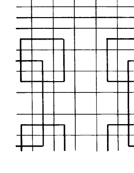
Figure 1: Pattern of increasing squares in a Robinson square tiling

Now the point is that the centres of the tiles of each of the six types form a model set based on an internal space which is $2$-adic. Very briefly the argument is as follows.

Starting with Fig. 1 and ignoring the actual square tiles themselves we have patterns of interlocking squares of increasing scale. Let’s call these the pattern-squares to distinguish them from the actual tiling squares. The vertices of the smallest scale pattern-squares (order 1) form the vertices of a lattice $L^{\prime}$ once one of them, say $c_{1}=(0,0)$, has been chosen as the origin. It is convenient to introduce the larger lattice $L=\frac{1}{2}\cdot L^{\prime}$ which we can identify with $\mathbb{Z}^{2}$. The locations of the vertices of the increasingly scaled pattern-squares determine two sequences, $\{\alpha_{k}\}$ and $\{\beta_{k}\}$, composed out of the two numbers $\{\pm 1\}$ as follows: the vertices of the pattern-squares of order $k$ (side-length $2^{k}$) are the points of a coset

$$L_{k}:=c_{k}+2^{k}L.$$ (10)

where

$$c_{k}=(\alpha_{0}+\alpha_{1}2+\dots,+\alpha_{k-2}2^{k-2},\beta_{0}+\beta_{1}2+\dots,+\beta_{k-2}2^{k-2})$$ (11)

for $k=2,3,\dots$. Conversely, given two sequences $\alpha,\beta$ of $\pm 1$’s we can use (11) and (10) to define the vertices of a suitable pattern of squares.

The pattern-squares themselves are determined by the condition that the points of $L_{k}$ are the centres of the squares of order $k-1$ for all $k>1$. This then establishes a coordinatization of the pattern-squares. Both the actual pattern of the pattern-squares and their coordinatization depend on the choice of our two sequences (more below).

Now looking again at the tiling squares, we distinguish the $6$ types of tiles according to their location in the pattern-squares. We list these here together with a description of the coordinates of the centres of their tiles:

• the “corner tiles” of the squares of order $1$;
  coordinates $L_{1}=2L$;  density $\frac{1}{4}$;

• the “corner tiles” of all squares of all higher orders;
  coordinates $\bigcup_{k\geq 2}c_{k}+2^{k}L$;  density $\frac{1}{12}$

• “cross tiles” where edges of two different orders of pattern squares meet (actually these orders always differ by exactly $1$);
  coordinates:
  $\left(\bigcup_{k\geq 3}c_{k}+(\pm 2^{k-2},\pm 2^{k-3})+2^{k}L\right)\cup\left(\bigcup_{k\geq 3}c_{k}+(\pm 2^{k-3},\pm 2^{k-2})+2^{k}L\right)$;
  density $\frac{1}{6}$;

• “edge ” squares, which contain part of a single edge of a pattern-square, except those in which are exactly in the middle of an edge;  density $\frac{1}{6}$;

• “edge ” squares, which contain part of a single edge of a pattern-square and which are exactly in the middle of an edge;  density $\frac{1}{6}$;

• blank tiles, with no part of any edge in them;  density $\frac{1}{6}$.

Observe that each of these sets is a countable union $w_{j}$ of cosets of the form $a+2^{k}L$. Let us replace each of these by the corresponding $2$-adic clopen set $a+2^{k}\cdot\mathbb{Z}_{2}^{2}$. In this way we get $6$ open sets $W_{j},\;j=1,\dots,6$, whose closures, being closed subsets of the compact group ${\mathbb{Z}_{2}^{2}}$, are compact with non-empty interiors. Finally we can describe the centres of the squares of type $j$ as

$$\{x\in\mathbb{Z}^{2}\mid x\in W_{j}\}$$ (12)

which, unlikely as it appears, is a model set under the scheme

$$\begin{array}[]{ccccc}\mathbb{R}^{2}&\stackrel{{\scriptstyle\pi_{1}}}{{\longleftarrow}}&\mathbb{R}^{2}\times{\mathbb{Z}_{2}^{2}}&\stackrel{{\scriptstyle\pi_{2}}}{{\longrightarrow}}&G\\ &&\cup&&\\ &&\mathbb{Z}^{2}&&\end{array}$$ (13)

where $\mathbb{Z}^{2}$ is embedded into $\mathbb{R}^{2}\times{\mathbb{Z}_{2}^{2}}$ diagonally: $x\mapsto(x,x)$.

The entire tiling is determined by the vertices of the various squares and hence by the window

$$W:=\bigcup_{k=1}^{\infty}c_{k}+2^{k}\mathbb{Z}_{2}^{2}.$$ (14)

Evidently $W$ is an open subset of   $\mathbb{Z}_{2}^{2}$. Let $w\in\overline{W}\backslash W$. Then for each $m\in\mathbb{Z}_{+}$, $w+2^{m}~{}\mathbb{Z}_{2}^{2}$ meets $W$, so $w\equiv c_{k}\;{\rm mod}\;2^{{\rm min}\{m,k\}}~{}\mathbb{Z}_{2}^{2}$ for some $k=k(m)$. If $k\leq m$ then $w\in c_{k}+2^{k}\mathbb{Z}_{2}^{2}\subset W$. Thus $k>m$ and $w\equiv c_{k(m)}{\rm mod}\;2^{m}\;\mathbb{Z}_{2}^{2}$. It follows that $w$ is the limit of some subsequence of the $\{c_{k}\}$. Since the entire sequence evidently converges (in the $p$-adic topology, of course!) to some $c=(a,b)$, where $a=\sum\alpha_{k}2^{k}$ and similarly for $b$, we see that $w=c$ and so $\partial W=\{c\}$. Thus the model set of all vertices is regular, and even generic provided that $c\notin\mathbb{Z}^{2}$.

More generally, one may expect this $p$-adic topologies to arise whenever there is a self-similarity $\theta:L\rightarrow L$ for which $\theta(L)\subset L$, but $\theta(L)\neq L$.

In [7] we also see the appearance of mixed $p$-adic and real spaces as the internal spaces. Beyond these types we are not aware of any interesting examples, though they may well exist.

5 Analytic side

The transition from an inherently discete picture on the physical side to something inherently far more continuous on the internal side is made via H. Weyl’s theory of uniform distribution.

Let us assume that we have a model set $\Lambda$. Now consider the following question. Suppose that we take a ball $B_{R}(0)$ of radius $R$ about the origin in $\mathbb{R}^{d}$ and look at $\Lambda_{R}:=\Lambda\cap B_{R}(0)$. Then we can ask how $\Lambda_{R}^{*}$ is distributed over $W$. We say that the sets $\Lambda_{R}^{*}$ are uniformly distributed if for each open set $U\subset W$ we have

$$\lim_{R\to\infty}\frac{{\rm card}(\Lambda_{R}^{*}\cap U)}{\mu(W)}\;=\;\mu(U)/\mu(W)$$ (15)

where $\mu$ is Haar measure on $G$.

Theorem 2

[35, 19] If $\Lambda$ is regular then the sets $\Lambda_{R}^{*}$ are uniformly distributed over $W$.

Let $f^{*}:G\longrightarrow\mathbb{C}$ be any function. We define $f:L\longrightarrow\mathbb{C}$ by $f(x)=f^{*}(x^{*})$. If $f^{*}$ is supported on the window $W$ then evidently $f$ is supported on the model set $\Lambda$. If $f^{*}$ is continuous (which is the case of interest) then this is iff.

Theorem 3

(Weyl) [39] If $\Lambda$ is regular and $f^{*}$ is continuous then

$$\lim_{R\to\infty}\frac{1}{{\rm card}(\Lambda_{R})}\sum_{x\in\Lambda_{R}}f(x)\;=\;\frac{1}{{\rm vol}(W)}\int_{W}f^{*}(u)d\mu(u)$$ (16)

Since $W$ has boundary of measure zero, it is not necessary to insist that $f^{*}$ (which is supported on $W$) be continuous on all of internal space, only on the window $W$.

In this way discrete averaging on the model set is transformed into integration on the window. This process was used in [4] to determine the existence of invariant measures on internal space in the presence of self-similarity on the quasi-crystal. We briefly explain this. We assume here that internal space is $\mathbb{R}^{n}$ for some $n$.

A self-similarity of $\Lambda$ is an affine linear mapping $t=t_{Q,v}$

$$t_{Q,v}\;:\quad x\mapsto Qx+v$$ (17)

on $\mathbb{R}^{d}$ that maps $\Lambda$ into itself, where $Q$ is a (linear) similarity and $v\in\mathbb{R}^{d}$. Thus $Q=qR$, i.e. it is made up of an orthogonal transformation $R$ and an inflation factor $q$.

Let $t_{Q,v}$ be a self-similarity of $\Lambda$. Since $\Lambda$ is uniformly discrete, we must have $|q|\geq 1$. We will assume $|q|>1$ and that $QL=L$. We are interested in the entire set of affine inflations with the same similarity factor $Q$.

Note that $Q$ naturally gives rise to an automorphism $\tilde{Q}$ of the lattice $\tilde{L}$, i.e. an element of ${\rm GL}_{\mathbb{Z}}(\tilde{L})$, and a linear mapping $Q^{*}$ of $\mathbb{R}^{n}$ that maps $W$ into itself. From the arithmetic nature of $\tilde{Q}$ we deduce that the eigenvalues of $Q$ and $Q^{*}$ are algebraic integers and from the compactness of $W$ that $Q^{*}$ is contractive.

Define

$$W_{Q}\;:=\;\{u\in\mathbb{R}^{n}\mid Q^{*}W+u\subset W\}\,,$$ (18)

We say that $Q$ is compatible with $\Lambda$ if $\mbox{int}(W_{Q})\neq\emptyset$. Assuming that this is the case (not a strong assumption) , then the set ${\cal T}_{Q}$ of affine inflations with the same similarity $Q$ is the set of mappings $t_{Q,v}:x\mapsto Qx+v$, where $v$ runs through the set

$$T\;=\;T_{Q}\;:=\;\{v\in L\mid v^{*}\in W_{Q}\}\,.$$ (19)

Theorem 4

If $Q$ is a self-similarity and the above assumptions on $Q$ apply then there is a unique absolutely continuous positive measure $\mu$ on internal space, supported on $W$, satisfying:

• $\mu(W)=1$;

• $\mu$ is invariant in the sense that, if we define $t^{*}_{v}\cdot\mu_{f}$ by $t^{*}_{v}\cdot\mu(Y)=\mu((t^{*}_{v})^{-1}(Y))$, then

  $$\mu\;=\;\lim_{s\to\infty}\frac{1}{\mbox{\small$\#$}\left(T\cap B_{s}(0)\right)}\sum_{v\in T\cap B_{s}(0)}t^{*}_{v}\cdot\mu_{f}~{}.$$ (20)

The similarity of this measure to Hutchison measures in the context of iterated function systems is not coincidental. In fact, if we restrict to the ball $B_{s}(0)$ then the $\{t_{v}^{*}\}$ form a finite set of contractions which is indeed an iterated function system. For more on this and invariant density functions on model sets see [4].

The type of limit averaging involved here is a very natural one from the point of view of physical situations, representing the transition from the world of sets finite in extent to the ideal world of infinitely extended point sets.

Although no one to our knowledge has made any use of it, it is interesting to use Weyl’s theorem to transfer the structure of $L^{2}(W)$ to a space of similar objects on $\Lambda$. Namely, the space of continuous functions on $W$ leads to a space

$${\cal C}={\cal C}(\Lambda)$$ (21)

of funtions on $\Lambda$ via the mapping ^∗. Then the usual inner product $\langle f,g\rangle=\int_{W}\overline{f^{*}(u)}g^{*}(u)du=\langle{\overline{f}},g\rangle_{W}$ defines an inner product on ${\cal C}$ and we can complete this space in order to get a Hilbert space $\overline{\cal C}$ isomorphic to $L^{2}(W)$. Of course the elements of $\overline{\cal C}$ can no longer be interpreted as functions on $\Lambda$ since functions on $\Lambda$ that differ by a function whose absolute square has limit average sum equal to $0$ are identified.

6 Dynamical systems side

So far we have looked at one model set in isolation. Now we move on to consider families of model sets. We start with a number of definitions and results. All of these may be found in the paper of M. Schlottmann [36] on which we have relied heavily here. Many are well-known in the context of tilings for which a recent reference with a good bibliography is [38]. In this section all point sets under discussion are assumed to be Delone sets in $\mathbb{R}^{d}$.

Two Delone sets $S,S^{\prime}$ in $\mathbb{R}^{d}$ are locally isomorphic (or some people say locally indistinguishable) if, up to translations, every patch of either of them occurs in the other. Thus on any finite scale, up to translation, the two sets are indistinguishable. Given a Delone set $S\subset\mathbb{R}^{d}$ we can look at its local isomorphism class (LI class) ${\rm LI}(S)$, namely all point sets locally isomorphic to it.

We denote by ${\cal X}(r)$ the set of all Delone sets of $\mathbb{R}^{d}$ for which the minimum separation between distinct points is at least $r$. We assume in the rest of this section that $r>0$ has been fixed.

We define a Hausdorff topology on ${\cal X}(r)$ as follows: two sets $S,S^{\prime}\in{\cal X}(r)$ are “close” if for some large compact set $K\subset\mathbb{R}^{d}$ and some small $\epsilon$ we have

$$(v+S)\cap K=S^{\prime}\cap K$$ (22)

for some $v\in\mathbb{R}^{r}$ with $|v|<\epsilon$. More precisely we define a uniformity ${\cal U}$ on ${\cal X}(r)$ using as the sets $U(K,\epsilon)$ of uniformity the set of pairs $(S,S^{\prime})$ satisfying (22).

Theorem 5

[32, 38, 36] With respect to this topology ${\cal X}(r)$ is a complete Hausdorff space.

Let $S\in{\cal X}(r)$. Then $\mathbb{R}^{d}$ acts on ${\rm LI}(S)$ by translation and in particular the entire orbit $[S]$ of $S$ lies in ${\rm LI}(S)$. This action is continuous and hence extends also to an action on the closure $\overline{{\rm LI}(S)}$ of ${\rm LI}(S)$. The relationship between orbits and LI classes can be summed up by

$$S\in[S]\subset{\rm LI}(S)\subset\overline{[S]}=\overline{{\rm LI}(S)}.$$ (23)

The second inclusion follows easily from the definitions. The inclusions may, according to the situation, be strict or actual equalities. For a lattice there is only one orbit in its LI class. For general model sets the situation is very different, as we shall see.

Recall that a Delone set $S$ is said to be of finite local complexity if the closure of $S-S$ is discrete. Finite local complexity is a property that is inherited by whole LI classes.

Theorem 6

An LI class is pre-compact (i.e its completion is compact) iff it has finite local complexity.

Thus, if $S$ is a Delone set of finite local complexity we obtain a dynamical system ${\cal D}(S)$:

$$\mathbb{R}^{d}\times\overline{[S]}\longrightarrow\overline{[S]}.$$ (24)

In the sequel we will use the symbols like ${\cal D}(S)$ to denote both the dynamical system itself and the corresponding defining space $\overline{[S]}$.

Theorem 7

Let $S$ be a Delone set of finite local complexity. The following are equivalent:

• $S$ is repetitive;

• $[S]={\rm LI}(S)$ is closed;

• The dynamical system ${\cal D}(S)$ is minimal.

We recall that minimal means that every $\mathbb{R}^{d}$ orbit is dense.

Since generic model sets are repetitive, this leads to a very nice result:

Theorem 8

Let $\Lambda$ be a generic model set. Then its LI class ${\rm LI}(\Lambda)$ is a compact Hausdorff space and under the action of translation under $\mathbb{R}^{d}$ it becomes a minimal dynamical system, ${\cal D}(\Lambda)$.

This is the first of the dynamical systems that we wish to consider. Its rather abstract form is better understood by relating it to a more accessible dynamical system.

To this end, let $\Lambda=\Lambda(W)=\{x\in L\mid x^{*}\in W\}$ be a model set. Each element $(u,v)$ of the group $\mathbb{R}^{d}\times G$ can be used to form a new model set

$$\Lambda(W,u,v)\;:=\;u+\{x\in L\mid x^{*}\in-v+W\}.$$ (25)

If $(u,v)\in{\tilde{L}}$ then $v=u^{*}$ and we can rewrite this as $\{u+x\in L\mid(u+x)^{*}\in W\}$, which is just $\Lambda$ again. Thus we get a whole family of model sets parametrized by $\mathbb{T}:=(\mathbb{R}^{d}\times G)/{\tilde{L}}$ with $\mathbb{R}^{d}\times G$ acting on it. This is the second dynamical system. Its points correspond to the model sets $\Lambda(W,u,v)$. This is the so-called torus parametrization introduced by Baake et al. in [3]. We use the same terminology in the more general context here, although in general $\mathbb{T}$ is not a torus!

The action of $\mathbb{R}^{d}$ on $\mathbb{T}$, $(x,y+{\tilde{L}})\mapsto x+y+{\tilde{L}}$, is a faithful transcription of the operation of translation in physical space, so the orbits of $\mathbb{R}^{d}$ on $\mathbb{T}$ correspond to model sets that differ only by translation. The action of $G$ on $\mathbb{T}$ corresponds to translating the window around.

Theorem 9

Let $\Lambda$ be a generic model set. Then

$$\mathbb{R}^{d}\times\mathbb{T}\longrightarrow\mathbb{T}$$ (26)

is a minimal uniquely ergodic dynamical system ${\cal D}_{\rm tor}$. The unique invariant probability measure is normalized Haar measure. The set of points of ${\cal D}_{\rm tor}$ corresponding to generic model sets is dense and indeed the set of points corresponding to the non-generic model sets is of the first category.

It is noteworthy that this dynamical system is independent of $W$ but the actual parametrization of model sets is clearly dependent on it.

So now given a generic model set $\Lambda$, there are two dynamical systems for the group $\mathbb{R}^{d}$, one ${\cal D}(\Lambda)$ coming from the closure of the orbit of $\Lambda$ under action of $\mathbb{R}^{d}$ and another ${\cal D}_{\rm tor}$ coming from the torus parametrization. Not surprisingly they are related, but rather surprisingly this relation is somewhat subtle. All the elements of ${\cal D}(\Lambda)$ are, by definition, in the same LI class. The same is not the case for the model sets parametrized by ${\cal D}_{\rm tor}$. Indeed, $\Lambda$ is generic, but translating the window around is bound to produce model sets that are not generic. These non-generic model sets are not locally isomorphic to the regular ones, because they have certain special local configurations of points that are related to the boundaries of their windows.

Theorem 10

[36] Let $\Lambda$ be a generic model set. Then there is a continuous surjective mapping

$$\beta:{\cal D}(\Lambda)\longrightarrow{\cal D}_{\rm tor}$$ (27)

which is $\mathbb{R}^{d}$-equivariant and which maps $\Lambda$ onto the point $0$ of the torus. Furthermore, for each of the points of ${\cal D}_{\rm tor}$ which parametrize generic model sets, the preimage in ${\cal D}(\Lambda)$ consists of a unique point.

This mapping comes about as follows: Let $\Lambda^{\prime}\in{\cal D}(\Lambda)$. First suppose that $\Lambda^{\prime}\subset L$. Then it is not hard to see that $\bigcap_{x\in\Lambda^{\prime}}(W-x^{*})$ is a single point, call it $b(\Lambda^{\prime})$. Furthermore, for all $u\in L$, $b(\Lambda^{\prime}-u)=b(\Lambda^{\prime})+u^{*}$. Now for arbitrary $\Lambda^{\prime}\in{\cal D}(\Lambda)$, we can always find $v\in\mathbb{R}^{d}$ with $\Lambda^{\prime}-v\subset L$. This $v$ is nothing like unique but it follows from what we have just said that the pair $\beta(\Lambda^{\prime}):=(v,b(\Lambda^{\prime}-v))$ is unique ${\rm mod}~{}{\tilde{L}}$, and this is the mapping that we require.

Using these facts it can be established that

Theorem 11

[36] Assume that $\Lambda$ is a regular and generic model set. Then ${\cal D}(\Lambda)$ is uniquely ergodic and furthermore $L^{2}({\cal D}(\Lambda))$ and $L^{2}({\cal D}_{\rm tor})$ are isometrically isomorphic as $\mathbb{R}^{d}$-spaces.

The importance of this is that it shows that from the spectrum of ${\cal D}_{\rm tor}$ being discrete, which it surely is since $\mathbb{T}$ a compact abelian group, it follows that the spectrum of ${\cal D}(\Lambda)$ is also discrete. It is from this that the pure point diffractivity of $\Lambda$ can be deduced. In the final section we briefly describe how this happens.

7 Diffraction

The theoretical framework for the discussion of diffraction has been very well described in several places. The two papers of A. Hof [17, 18] are standards and there are also good descriptions in [15, 6]. Here we just quickly formulate the definitions.

Let $\Lambda$ be a regular model set and define the (tempered) distribution

$$\delta_{\Lambda}:=\sum_{x\in\Lambda}\delta_{x}\;,$$ (28)

where $\delta_{x}$ is the Dirac measure at $x$. For each $s>0$ we calculate the auto-correlation of $\delta_{\Lambda}$ restricted to the ball of radius $s$:

$$\delta_{\Lambda\cap B_{s}(0)}*\tilde{\delta}_{\Lambda\cap B_{s}(0)}\;=\;\sum_{x,y\in\Lambda\cap B_{s}(0)}\delta_{x-y}\;,$$ (29)

where, as usual, the over-tilde indicates changing the sign of the argument. The limit as $s$ goes to infinity of the volume-averaged auto-correlation of this measure, which exists for model sets, is the auto-correlation measure of $\Lambda$ (its so-called Patterson function):

$$\gamma\;=\;\lim_{s\to\infty}\frac{1}{{\rm vol}(B_{s}(0))}\sum_{x,y\in\Lambda_{s}}\delta_{x-y}~{}.$$

This limit, taken in the vague topology, converges to a tempered distribution (i.e. this limit exists when taken against rapidly decreasing test functions). Its Fourier transform is a positive measure $\hat{\gamma}$ (a result of Bochner’s theorem applied to the positive definite distribution $\gamma$) which is the diffraction pattern of $\Lambda$. The measure decomposes into a point part and a continuous part. The point part of this measure is the Bragg spectrum of $\Lambda$. The model set has pure point spectrum if the continuous part is the trivial $0$-measure.

The complexity of the definition makes it hard to discover the nature of the diffraction pattern, in particular whether or not we have pure-point diffraction or not. One approach has been to use the ergodic theory outlined above, and indeed it is able to give the main result:

Theorem 12

[36] Any regular model set has pure point spectrum. Furthermore this spectrum is supported on the projection into Fourier space on the physical side of the dual of the compact group $\mathbb{T}$ (5), i.e.  it has the form

$${\hat{\gamma}}\;=\;\sum_{k\in{\hat{\mathbb{T}}}}w(k)\delta_{{\hat{\pi}}_{1}(k)}$$ (30)

The proof of this is based on an idea of Dworkin [12]. The argument is spelled out in [18] and we repeat it here since otherwise it is difficult to see the connection between dynamical systems and diffraction.

We can assume that $\Lambda$ is generic since translation of the window does not alter the qualitative nature of the diffraction. The next step is to replace $\delta_{\Lambda}$ by a smooth approximation to it. To this end, let $b:\mathbb{R}^{d}\longrightarrow\mathbb{R}_{\geq 0}$ be a smooth function whose support is contained in the ball $B_{r}(0)$ of radius $r$, where $B_{2r}(0)\cap(\Lambda-\Lambda)=\{0\}$. Define a function $\psi:{\cal D}(\Lambda)\longrightarrow\mathbb{R}$ by

$$\psi(\Lambda^{\prime})\;=\;\int_{\mathbb{R}^{d}}b(-u)\delta_{\Lambda^{\prime}}(u)du,$$ (31)

which is continuous on ${\cal D}(\Lambda)$. The action of $\mathbb{R}^{d}$ on $[\Lambda]$ gives rise to a corresponding action $x\mapsto T_{x}$ on the space of functions on the orbit $[\Lambda]$ of $\Lambda$ under translation.

For each $x\in\mathbb{R}^{d}$ we have

$$T_{x}\,\psi(\Lambda)=\int_{\mathbb{R}^{d}}b(-u)\delta_{-x+\Lambda}(u)du=\int_{\mathbb{R}^{d}}b(-u)\delta_{\Lambda}(x+u)du=b*\delta_{\Lambda}(x)\;,$$ (32)

which shows that the function $\sigma^{(b)}\;:\mathbb{R}^{d}\longrightarrow\mathbb{C}$ defined by $x\mapsto T_{x}(\psi)(\Lambda)$ is obtained by centering a copy of $b$ at each point of $\Lambda$.

Now consider the autocorrelation of $\sigma^{(b)}$:

$$\begin{array}[]{ccc}\gamma^{(b)}(x)&=&\lim_{s\to\infty}\frac{1}{{\rm vol}(B_{s}(0))}\int_{B_{s}(0)}\overline{T_{x+y}(\psi)(\Lambda)}T_{y}(\psi)(\Lambda)dy\\ \\ &=&\int_{{\cal D}(\Lambda)}\overline{T_{x}(\psi})\psi\,d\mu\;=\;(T_{x}\psi,\psi).\end{array}$$ (33)

The main point here is the use of the Birkhoff ergodic theorem and the ergodicity of the action of $\mathbb{R}^{d}$ on ${\cal D}(\Lambda)$ to replace the integral over $\mathbb{R}^{d}$ by an integral over ${\cal D}(\Lambda)$. Note that the uniqueness of ergodicity and the continuity of $\psi$ is needed here to guarantee the statement for all $x$ rather than a.e. ([14], Sec. 3.2).

In view of Theorem 11, we have a Fourier expansion of $\psi$ in terms of the eigenfunctions for the action of $\mathbb{R}^{d}$: $\psi\;=\;\sum a_{\lambda}\phi_{\lambda}$, where $\phi_{\lambda}$ is the eigenfunction for the character $x\mapsto e^{2\pi i\lambda.x}$ on $\mathbb{R}^{d}$. Thus $(T_{x}\psi,\psi)=\sum|a_{\lambda}|^{2}e^{2\pi i\lambda.x}$ and taking Fourier transforms we have

$${\hat{\gamma}^{(b)}}=\sum|a_{\lambda}|^{2}\delta_{\lambda}$$ (34)

which is a pure point measure on $\mathbb{R}^{d}$.

On the other hand we know that $\sigma^{(b)}=b*\delta_{\Lambda}$ whose autocorrelation can be calculated directly as $b*{\tilde{b}}*\gamma$ and so ${\hat{\gamma}^{(b)}}=|\hat{b}|^{2}{\hat{\gamma}}$. Finally, taking a sequence of bump functions $\{b\}$ converging in the vague topology to $\delta_{0}$ we obtain the required pure-point nature of the diffraction pattern.

Theorem 12 is qualitative in nature. The quantitative counterpart is this:

Theorem 13

[26] Let $k\in{\hat{\mathbb{T}}}$ and let $\chi$ denote the characteristic (or indicator) function of $W$. Then $w(k)=|{\hat{\chi}}(-{\hat{\pi}_{2}}(k))/{\rm vol}(W)|^{2}$.

There are a number of variations on this theme that are worthwhile mentioning. First we may imagine replacing the simple sum (28) by a weighted sum

$$\delta_{\Lambda}^{\omega}:=\sum_{x\in\Lambda}\omega(x)~{}\delta_{x}\;,$$ (35)

where $\omega:\Lambda\longrightarrow\mathbb{C}$ is some function.

Theorem 14

If $\Lambda$ is a regular model set and if $\omega\in{\cal C}(\Lambda)$ (see (21)) then the weighted point distribution is pure point diffractive.

Next we consider the case that our points of $\Lambda$ are considered stochastically:

$$\delta_{\rm stochastic}:=\sum_{x\in\Lambda}\eta(x)~{}\delta_{x}\;,$$ (36)

where the $\eta(x)$ form a collection of independent identically distributed random variables that take the values $1,0$ (indicating occupancy or not of the respective model set sites) with the probability of occupancy being $p$:

Theorem 15

[5] Let $\Lambda$ be a regular model set and let $\eta$ be as above with the mean and second moment equal to $m_{1}$ and $m_{2}$ respectively. Then the autocorrelation of $\Lambda$ and that of its stochastic version are, with probability one, related by

$$\gamma_{\rm stochastic}\;=\;(m_{1})^{2}\,\gamma+d~{}(m_{2}-(m_{1})^{2})\delta_{0}\,$$ (37)

with Fourier transforms

$$\hat{\gamma}_{\rm stochastic}\;=\;(m_{1})^{2}\,\hat{\gamma}+d~{}(m_{2}-(m_{1})^{2})\,,$$ (38)

where $d$ is the density per unit volume of the $\Lambda$.

Thus the pure point nature of $\Lambda$ is affected by at most the addition of a constant continuous background. More on this stochastic approach may be found in [5].

Yet a different variation is to allow the points of $\Lambda$ to be moved in some regular way.

Theorem 16

[18] Let $\Lambda$ be a regular model set and let $f:x\mapsto(f_{1}(x),\dots,f_{d}(x))$ be some mapping of $\Lambda$ into $\mathbb{R}^{d}$, where each $f_{i}\in{\cal C}(\Lambda)$ (see (21)). Then the set $\Lambda_{f}:=\{x+f(x)\mid x\in\Lambda\}$ is pure point diffractive.

These variations can be combined in the obvious ways.

The problems of determining which point sets are pure point diffractive is a fascinating and challenging one which is still wide open. The examples above show how much model sets can be modified without serious damage to their diffractive properties. Obviously adding or removing points whose average density is $0$ also does not alter the diffraction. But there are point sets that are even more remote that are diffractive. One example is the set of visible points of a lattice. Given a lattice $L$ in $\mathbb{R}^{d}$ its visible points are those points $x\in L$, $x\neq 0$, satisfying $\mathbb{Q}x\cap L=\mathbb{Z}x$. What is interesting about the visible points is that they do not form a Delone set (they are not relatively dense in $\mathbb{R}^{d}$). In fact, for each $r>0$, the set of holes of radius exceeding $r$ has positive density. However,

Theorem 17

[6] The set of visible points of any lattice of rank at least $2$ is pure point diffractive.

7.1 Comment

In this paper we have considered point sets in $\mathbb{R}^{d}$ that are constructed through the method of projection from an embedding group and a lattice. We have assumed that the embedding group is of the form $\mathbb{R}^{d}\times G$ where $G$ is a locally compact abelian group, which, in view of Theorem 1, is fairly natural. However, it is possible to study model sets in the situation where the ‘physical space’ has been replaced by an arbitrary locally compact abelian group without losing many of the most interesting properties. In particular the diffraction results of Theorem 12 have formulations in this generality [36].

References

- [1] M. Baake, “A guide to mathematical quasicrystals”, in: Quasicrystals, eds. J. B. Luck, M. Schreiber, P. Häussler, Springer, (1998).
- [2] M. Baake, P. Kramer, M. Schlottmann, and D. Zeidler, “Planar patterns with five-fold symmetry as sections of periodic structures in -space”, Int. J. Mod. Phys. B4(1990), 2217-2268.
- [3] M. Baake, J. Hermisson, and P. Pleasants, “The torus parametrization of quasiperiodic LI-classes”, J. Phys A: Math. Gen. 30(1997), 3029-3056.
- [4] M. Baake and R. V. Moody, “Self-similarities and invariant densities for model sets”, in: Algebraic Methods and Theoretical Physics, ed. Y. St. Aubin, Springer, New York (1997), in press.
- [5] M. Baake and R. V. Moody, “Diffractive Point Sets with Entropy”, J.Phys. A (to appear), 1998.
- [6] M. Baake, R. V. Moody, and P. Pleasants, Diffraction from visible lattice points and th power free integers, (preprint), 1998.
- [7] M. Baake, R. V. Moody, and M. Schlottmann, “Limit-periodic point sets as quasicrystals with -adic internal spaces, J.Phys. A: Math.Gen.31(1998), 5755-5765.
- [8] M. Baake and M. Schlottmann, “Geometric Aspects of Tilings and Equivalence Concepts”, in: Proc. of the 5th Int. Conf. on Quasicrystals, eds. C. Janot and R. Mossery, World Scientific, Singapore (1995), pp. 15–21.
- [9] N. Bourbaki, Topology, Vol. 1, Addison-Wesley, Reading (1966).
- [10] L. Chen, R. V. Moody, and J. Patera, “Non-crystallographic root systems”, Quasicrystals and Discrete Geometry, ed. J. Patera, Fields Institute Monographs, Vol. 10, AMS, Rhode Island (1998).
- [11] J. H. Conway and N. J. A. Sloane, Sphere packings, lattices and groups 2nd Ed., Springer, New York, Berlin (1998).
- [12] S. Dworkin, “Spectral theory and X-ray diffraction”, J. Math. Phys. 34(1993), 2965-2967.
- [13] V. Elser and N. J. Sloane, “A highly symmetric quasicrystal”, J. Phys. A: Math.Gen., 20(1987), 6161.
- [14] H. Furstenberg, Recurrence in ergodic theory and combinatorial number theory, Princeton University Press, Princeton, New Jersey, 1981.
- [15] F. Gähler and R. Klitzing, “The diffraction pattern of self-similar tilings”, in: The Mathematics of Long-Range Aperiodic Order, ed. R. V. Moody, NATO ASI Series C 489, Kluwer, Dordrecht (1997), pp. 141–74.
- [16] B. Grünbaum and G. C. Shephard, Tilings and Patterns, Freeman, New York (1987).
- [17] A. Hof, “On diffraction by aperiodic structures”, Commun. Math. Phys. 169(1995), 25-43.
- [18] A. Hof, “Diffraction by aperiodic structures”, in: The Mathematics of Long-Range Aperiodic Order, ed. R. V. Moody, NATO ASI Series C 489, Kluwer, Dordrecht (1997), pp. 239–68.
- [19] A. Hof, “Uniform distribution and the projection method”, in: Quasicrystals and Discrete Geometry, ed. J. Patera, Fields Institute Monographs, Vol. 10, AMS, 1998.
- [20] A. Katz and M. Duneau, “Quasiperiodic patterns and icosahedral symmetry”, J. Physique 47 (1986) 181–96.
- [21] P. Kramer, “Non-periodic central space filling with icosahedral symmetry using copies of seven elementary cells”, Acta Cryst. A38 (1982) 257–64.
- [22] P. Kramer and R. Neri, “On periodic and non-periodic space fillings of obtained by projection”, Acta Cryst. A40 (1984) 580–7, and Acta Cryst. A41 (1985) 619 (Erratum).
- [23] J. C. Lagarias, “Meyer’s concept of quasicrystal and quasiregular sets”, Comm. Math.Phys., 179(1996), 365-376.
- [24] J. C. Lagarias, “Mathematical Quasicrystals”, in: Directions in Mathematical Quasicrystals, eds. M. Baake and R. V. Moody, CRM Monograph series, AMS, Rhode Island (1998), in preparation.
- [25] Y. Meyer, Algebraic numbers and harmonic analysis, North Holland, Amsterdam (1972).
- [26] Y. Meyer, Quasicrystals, Diophantine approximation, and algebraic numbers, in: Quasicrystals and Beyond, eds F. Axel and D. Gratias, Les Editions de Physique, Springer-Verlag, 1995.
- [27] R. V. Moody, “Meyer sets and their duals”, in: The Mathematics of Long-Range Aperiodic Order, ed. R. V. Moody, NATO ASI Series C 489, Kluwer, Dordrecht (1997), pp. 403–41.
- [28] R. V. Moody and J. Patera, “Quasicrystals and Icosians”, J. Phys. A: Math. Gen., 26 (1993) 2829-2853.
- [29] J. Neukirch, “The -adic numbers”, in: Numbers, eds. H.-D. Ebbinghaus et al., Springer, New York (1990), pp. 155–178.
- [30] R. Penrose, “Remarks on tiling: Details of a -aperiodic set”, in: The Mathematics of Long-Range Aperiodic Order, ed. R. V. Moody, NATO ASI Series C 489, Kluwer, Dordrecht (1997), pp. 467–97.
- [31] C. Radin, “The pinwheel tilings of the plane”, Annals of Mathematics, 139, 661-702.
- [32] C. Radin and M. Wolff, “Space tilings and local isomorphism”, Geometriae Dedicata 42(1992), 355-360.
- [33] R. M. Robinson, “Undecidability and nonperiodicity of tilings of the plane”, Inv. Math. 44 (1971) 177–209.
- [34] D. S. Rokshar, D. C. Wright, and N. D. Mermin, “Scale equivalence of quasicystallographic space groups”, Phys. Rev., B37 (1988) 8145–8149.
- [35] M. Schlottmann, “Cut-and-project sets in locally compact abelian groups”, in: Quasicrystals and Discrete Geometry, ed. J. Patera, Fields Institute Monographs, Vol. 10, AMS, Rhode Island (1998), in press.
- [36] M. Schlottmann, “Generalized model sets and dynamical systems”, to appear in: Directions in Mathematical Quasicrystals, eds. M. Baake and R. V. Moody, CRM Monograph series, AMS, Rhode Island (1998), in preparation.
- [37] M. Senechal, “Quasicrystals and geometry”, Cambridge U. Press, 1995.
- [38] B. Solomyak, “Dynamics of self-similar tilings”, Ergod. Th. & Dynam. Syst. 17 (1997) 695–738.
- [39] H. Weyl, “Uber die Gleichungverteilung von Zahlen mod. Eins”, Math. Ann. 77 (1916) 313–352.