Diffraction of the Dart-Rhombus Random Tiling

Moritz Höffe

Institut für Theoretische Physik, Universität Tübingen, Auf der Morgenstelle 14, D-72076 Tübingen, Germany

  Abstract
       The diffraction spectrum of the dart-rhombus random tiling of the plane is derived in rigorous terms. Using the theory of dimer models, it is shown that it consists of Bragg peaks and an absolutely continuous diffuse background, but no singular continuous component. The Bragg part is given explicitly. Keywords: Diffraction, Diffuse scattering, Random tilings, Dimer models, Quasicrystals  

1. Introduction

Structure models of quasicrystals are usually based on the asumption of either energetical or entropical stabilization of the material. Random tilings as possible structure models of the second kind where proposed [5] soon after the discovery of quasicrystals and studied thoroughly since, see e.g. [11, 16, 9] and references therein. Nonetheless, until today it is not yet clear which mechanism is dominating, although experiments are indicating a stochastic component in many cases [13]. Scaling arguments [10, 11] predict a singular continuous contribution to the diffraction spectrum for two-dimensional random tilings in addition to the usual Bragg part and continuous background. This should be visible in diffraction images of materials with so-called T-phases, see [1] and references therein, though it is not obvious how to distinguish the different contributions. This underlines the necessity of investigating the diffraction of random tilings in more detail.

In this article, we illustrate recently established results [2] by the so-called dart-rhombus tiling. This two-dimensional model has crystallographic symmetries and can be mapped onto the dimer model on the Fisher lattice. After introducing the tiling and the necessary mathematical tools, we calculate the two-point correlation functions and thereof the diffraction spectrum. As in other crystallographic examples, the spectrum can be shown to consist only of a Bragg part and an absolutely continuous background, i.e. there is no singular continuous component.

2. The dart-rhombus random tiling

The dart-rhombus tiling is a filling of the plane, without gaps and overlaps, with $60^{\circ}$-rhombi of side $1$ and darts made of two rhombus halves (Fig. 1).

Fig. 1: The dart-rhombus tiling as dimer model on the Fisher lattice. The dots represent the atomic scatterers.

In addition to the usual face-to-face condition, we impose an alternation condition on the rhombi, such that neighbouring rhombi of equal orientation are excluded. Finally, to avoid pathological lines of alternating darts, we demand that two neighbouring darts must not share a short edge. These rules force the darts to form closed loops in a background of alternating rhombi. The minimal total rhombus density obviously is $1/3$. This tiling can be mapped onto the fully packed dimer model on an Archimedian tiling known as Fisher’s lattice in the context of statistical mechanics. In order to control the densities of the different prototiles, we weigh them using activities $y_{i},z_{i}$ (Fig. 2), with $z_{i}=e^{\beta\mu_{i}}$ etc., where $\mu_{i}$ are chemical potentials and $\beta$ the inverse temperature.

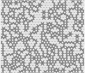
Fig. 2: Elementary cell of the Fisher lattice with activities assigned to each bond and a typical random tiling with $\rho_{1}=0.21$, $\rho_{2}=0.19$, $\rho_{3}=0.17$.

The grand-canonical partition function is therefore equal to the dimer generating function. For any periodic graph with even number of sites in the elementary cell, the latter can be computed as Pfaffian of the suitably activity-weighted adjacency matrix $\boldsymbol{A}$ [14]. The calculation of the Pfaffian is simplified considerably by imposing periodic boundary conditions, but in the infinite volume limit the result holds also for free ones [2, Lemma 1].

Let us denote the rhombus densities by $\rho_{i}$ ($i=1,2,3$) and the the dart densities by $\sigma_{j}$ ($j=1,\dots,6$). There are several constraints on the densities. Closed dart loops require equal densities of opposite darts:

$$\sigma_{1}=\sigma_{5},\quad\sigma_{2}=\sigma_{6},\quad\sigma_{3}=\sigma_{4}.$$ (1)

Moreover, as each dart is accompanied by a corresponding rhombus, the remaining rhombi occur with equal frequency owing to the alternation condition,

$$\rho_{1}-\sigma_{1}=\rho_{2}-\sigma_{2}=\rho_{3}-\sigma_{3}.$$ (2)

Including the normalization constraint (the sum of the densities is $1$), the number of independent parameters (activities or densities) reduces to three. We exploit this freedom by setting all activities except $z_{1},z_{2}$ and $z_{3}$ equal to $1$. The dart-rhombus tiling undergoes second order phase transitions at

$$1+z_{1}^{2}+z_{2}^{2}+z_{3}^{2} =2\max\{1,z_{1}^{2},z_{2}^{2},z_{3}^{2}\}\;\text{or}$$

$$z_{1}^{2}+z_{2}^{2}+z_{3}^{2} =2\max\{z_{1}^{2},z_{2}^{2},z_{3}^{2}\}$$

with logarithmic (Onsager type) or square root divergence (Kasteleyn type), respectively. The point of maximum entropy is fixed by symmetry to $\rho_{i}=\frac{1}{6}$, $\sigma_{j}=\frac{1}{12}$, where darts and rhombi occupy half of the tiling area each. For further details see [16, 12].

3. Diffraction theory

For simplicity, we assume kinematic diffraction in the Fraunhofer picture [4], i.e. diffraction at infinity from single-scattering. The diffracted intensity $\widehat{\gamma}_{\omega}$ (a positive measure) is calculated as Fourier transform of the autocorrelation $\gamma_{\omega}$ (see [2] for details). It is known that every positive measure admits a unique decomposition into three parts $\mu=\mu_{pp}+\mu_{sc}+\mu_{ac}$ with respect to Lebesgue’s measure, where $pp$, $sc$ and $ac$ stand for pure point, singular continuous and absolutely continuous [17]. In a diffraction spectrum, $\mu_{pp}$ are the Bragg peaks and $\mu_{ac}$ the usual diffuse background or Laue scattering. A singular continuous part can be encountered in 1D substitutional sequences, cf [6], and is also expected for 2D quasicrystalline random tilings [10, 11, 2].

Consider the so-called weighted Dirac comb [3]

$$\omega=\sum_{x\in\tilde{\Gamma}}w(x)\delta_{x}$$ (3)

on a lattice $\tilde{\Gamma}$, where $\delta_{x}$ is the unit point measure (Dirac measure) concentrated at $x$, and $w(x)\in\{0,1\}$ is chosen in order to obtain a specific member of the random tiling ensemble. Its autocorrelation $\gamma_{\omega}$ is (almost surely)

$$\gamma_{\omega}=\sum_{z\in\Delta}\nu(z)\delta_{z}.$$ (4)

Here, $\Delta=\tilde{\Gamma}-\tilde{\Gamma}=\tilde{\Gamma}$ is the set of difference vectors and the autocorrelation coefficient $\nu(z)$ can be calculated according to

$$\nu(z)\;=\;\lim_{R\to\infty}\frac{1}{{\rm vol}(B_{R})}\sum_{\stackrel{{\scriptstyle\scriptstyle y\in\Lambda_{R}}}{{\scriptstyle y+z\in\Lambda}}}\overline{w(y)}\,w(y+z)\,,$$ (5)

where $B_{R}$ is the ball of radius $R$ around the origin, $\Lambda_{R}=\Lambda\cap B_{R}$ and $\overline{\hphantom{x}}$ the complex conjugation. Thus, $\nu(z)$ is simply the probability of having two scatterers at distance $z$, which a.s. exists.

We use standard Fourier theory of tempered distributions, for our conventions see [2].

4. Diffraction of the dart-rhombus tiling

We decorate the tiling with point scatterers $\delta_{x}$ according to Fig. 1. More realistic atomic profiles can be handled with the convolution theorem [17, Ch. IX]. The scatterers may have complex strengths $h_{\rho_{i}}$, resp. $h_{\sigma_{j}}$, where the strengths of opposite darts are supposed to be equal. This constraint simplifies the calculations but is not necessary. The point set of all possible atomic positions is a Kagomé grid with minimal vertex distance $1/2$. We write it as triangular lattice $\Gamma$ with a rhombic elementary cell $E$ containing the nine scatterers positions for the different tiles (cf Fig. 2). Introducing basis vectors $e_{1}=(\sqrt{3},0)^{t}$, $e_{2}=1/2(\sqrt{3},3)^{t}$ for $\Gamma$ and $E$, the positions $p$ in $E$ (with corresponding density) are given by ($a=1/4(\sqrt{3},1)^{t}$, $b=1/4(\sqrt{3},-1)^{t}$)

$$p_{\rho_{1}}= \,3a, p_{\rho_{2}}= \,2a-b, p_{\rho_{3}}= \,a+b,$$

$$p_{\sigma_{1}}= \,a, p_{\sigma_{2}}= \,2a+b, p_{\sigma_{3}}= \,3a-b,$$ (6)

$$\quad p_{\sigma_{4}}= \,3a+b, p_{\sigma_{5}}= \,5a, p_{\sigma_{6}}= \,4a-b.$$

We now have to calculate the autocorrelation or the joint occupation probability of the dimers. As we will see, the autocorrelation coefficients can be split into a constant term and one decreasing with the distance between the scatterers. After taking the Fourier transform, the first will yield the Bragg peaks whereas the second will be responsible for the continuous part of the spectrum; we will show that this can be represented by a continuous function and hence contains no singular contribution.

Using Gibbs’ weak phase rule [18, 2], one can prove the ergodicity of the model and thus justify the calculation of the diffraction spectrum via the ensemble average.

Let $\eta_{\boldsymbol{kk}^{\prime}}$ be the occupation variable that takes the value $1$ if the bond between $\boldsymbol{k}$ and $\boldsymbol{k}^{\prime}$ is occupied and $0$ otherwise; $\bar{\eta}_{\boldsymbol{kk}^{\prime}}:=1-\eta_{\boldsymbol{kk}^{\prime}}$. As was shown in [2], the probability $P_{\alpha\beta}$ of bonds $\alpha$ and $\beta$ being occupied simultaneously is given by

$$P_{\alpha\beta}= \langle\eta_{\boldsymbol{k}_{\alpha}\boldsymbol{k}^{\prime}_{\alpha}}\eta_{\boldsymbol{k}_{\beta}\boldsymbol{k}^{\prime}_{\beta}}\rangle$$

$$= \langle\eta_{\boldsymbol{k}_{\alpha}\boldsymbol{k}^{\prime}_{\alpha}}\rangle\langle\eta_{\boldsymbol{k}_{\beta}\boldsymbol{k}^{\prime}_{\beta}}\rangle$$

$$+\langle\bar{\eta}_{\boldsymbol{k}_{\alpha}\boldsymbol{k}^{\prime}_{\alpha}}\bar{\eta}_{\boldsymbol{k}_{\beta}\boldsymbol{k}^{\prime}_{\beta}}\rangle-\langle\bar{\eta}_{\boldsymbol{k}_{\alpha}\boldsymbol{k}^{\prime}_{\alpha}}\rangle\langle\bar{\eta}_{\boldsymbol{k}_{\beta}\boldsymbol{k}^{\prime}_{\beta}}\rangle$$ (7)

$$= \,\rho_{\alpha}\,\rho_{\beta}$$

$$-A_{\boldsymbol{k}_{\alpha}\boldsymbol{k}^{\prime}_{\alpha}}A_{\boldsymbol{k}_{\beta}\boldsymbol{k}^{\prime}_{\beta}}(A^{-1}_{\boldsymbol{k}_{\alpha}\boldsymbol{k}_{\beta}}A^{-1}_{\boldsymbol{k}^{\prime}_{\alpha}\boldsymbol{k}^{\prime}_{\beta}}-A^{-1}_{\boldsymbol{k}_{\alpha}\boldsymbol{k}^{\prime}_{\beta}}A^{-1}_{\boldsymbol{k}^{\prime}_{\alpha}\boldsymbol{k}_{\beta}}),$$

with $\rho_{\alpha}$ the density of dimers that can occupy the bond $(\boldsymbol{k}_{\alpha}\boldsymbol{k}^{\prime}_{\alpha})$ and $\boldsymbol{A}$ the weighted adjacency matrix.

We consider the constant part of the autocorrelation first. Combining (4) and (4.) we get for the point set of scatterers with density $2/\sqrt{3}$

$$(\gamma_{\omega})_{const}=\omega_{\Gamma}*\bigg{(}\frac{2}{\sqrt{3}}\sum_{\tau,\tilde{\tau}\in\{\rho_{i},\sigma_{j}\}}\!\!\!(h_{\tau}h_{\tilde{\tau}}\tau\tilde{\tau})\delta_{p_{\tau}-p_{\tilde{\tau}}}\bigg{)},$$

where $*$ denotes convolution. Computing the Fourier transform with Poisson’s summation formula [2, Eq. 12] using (4.) and (1), the pure point part of the spectrum is (almost surely)

$$(\widehat{\gamma})_{pp}= \frac{4}{3}\sum_{(k,l)\in\Gamma^{*}}\bigg{|}h_{\rho_{1}}\rho_{1}+(-1)^{k}h_{\rho_{2}}\rho_{2}+(-1)^{l}h_{\rho_{3}}\rho_{3}$$

$$+2\cos{\textstyle\frac{\pi(k+l)}{3}}\Bigl{(}(-1)^{k+l}h_{\sigma_{1}}\sigma_{1}$$ (8)

$$+(-1)^{l}h_{\sigma_{2}}\sigma_{2}+(-1)^{k}h_{\sigma_{3}}\sigma_{3}\Bigr{)}\bigg{|}^{2}\delta_{(k,l)},$$

where $\Gamma^{*}$ is spanned by $e_{1}^{*}=\big{(}\frac{1}{\sqrt{3}},-\frac{1}{3}\big{)}$, $e_{2}^{*}=\big{(}0,\frac{2}{3}\big{)}$.

It remains to calculate the other part of (4.). $A_{\boldsymbol{k}_{\alpha}\boldsymbol{k}^{\prime}_{\alpha}}$ is nonvanishing only if $\boldsymbol{k}_{\alpha}$ and $\boldsymbol{k}^{\prime}_{\alpha}$ are connected; in this case $A_{\boldsymbol{k}_{\alpha}\boldsymbol{k}^{\prime}_{\alpha}}=\epsilon z_{\alpha}$, with $\epsilon=\pm 1$ according to the direction of the arrows in Fig. 2.

Since $\boldsymbol{A}$ is the adjacency matrix of a graph that is an $(m,n)$-periodic array of elementary cells with toroidal boundary conditions and therefore cyclic, it can be reduced to the diagonal form $\boldsymbol{\Lambda}=\text{diag}\{\lambda_{\boldsymbol{j}}\}$ by a Fourier-type similarity transformation with matrix $S_{\boldsymbol{kk}^{\prime}}=(mn)^{-1/2}\exp(2\pi i(k_{1}k^{\prime}_{1}/m+k_{2}k^{\prime}_{2}/n))$. $\boldsymbol{A}^{-1}$ is then determined by [8]

$$A^{-1}_{\boldsymbol{kk}^{\prime}}=\left(\boldsymbol{S\Lambda}^{-1}\boldsymbol{S}^{-1}\right)_{\boldsymbol{kk}^{\prime}}=\sum_{\boldsymbol{j}=(1,1)}^{(m,n)}S_{\boldsymbol{kj}}\lambda_{\boldsymbol{j}}^{-1}S^{\dagger}_{\boldsymbol{k}^{\prime}\boldsymbol{j}}\,.$$ (9)

In the infinite volume limit, the sums approach integrals (Weyl’s Lemma), and by introducing ${\boldsymbol{r}}=\boldsymbol{k}^{\prime}-\boldsymbol{k}$, $\varphi_{1}=2\pi ij_{1}/m$ etc. we obtain

$$A^{-1}_{\boldsymbol{kk}^{\prime}}=\frac{1}{4\pi^{2}}\int\limits_{0}^{2\pi}\int\limits_{0}^{2\pi}\lambda^{-1}(\varphi_{1},\varphi_{2})e^{i\boldsymbol{\varphi}\cdot{\boldsymbol{r}}}d\varphi_{1}d\varphi_{2}.$$ (10)

To determine $\lambda^{-1}$, observe that the inverse of

$$\lambda=\begin{pmatrix}0&z_{1}&z_{3}&0&-e^{-i\varphi_{1}}&0\\ -z_{1}&0&z_{2}&0&0&-e^{-i\varphi_{2}}\\ -z_{3}&-z_{2}&0&1&0&0\\ 0&0&-1&0&z_{3}&z_{2}\\ e^{i\varphi_{1}}&0&0&-z_{3}&0&z_{1}\\ 0&e^{i\varphi_{2}}&0&-z_{2}&-z_{1}&0\end{pmatrix}$$

can be computed easily by any computer-algebra package but unfortunately does not fit onto this page.

Defining the coupling function $[x,y]_{p_{1}p_{2}}$ for two dimers in elementary cells at distance $\boldsymbol{r}=xe_{1}+ye_{2}$, with $(x,y)\in\mathbb{Z}^{2}$, where the dimers occupy positions $p_{1}$, resp. $p_{2}$ in each elementary cell, we rewrite (10) in more explicit form

$$[x,y]_{p_{1}p_{2}}=\frac{1}{4\pi^{2}}\int\limits_{0}^{2\pi}\int\limits_{0}^{2\pi}\frac{g(p_{1},p_{2},\varphi_{1},\varphi_{2})e^{i\boldsymbol{\varphi}\cdot\boldsymbol{r}}}{\det\left(\lambda(\varphi_{1},\varphi_{2})\right)}d\varphi_{1}d\varphi_{2},$$

where the determinant of $\lambda$ is given by

$$\det(\lambda)=a+2b\cos\varphi_{1}+2c\cos\varphi_{2}+2d\cos(\varphi_{1}-\varphi_{2}),$$

with $a=z_{1}^{4}+z_{2}^{4}+z_{3}^{4}+1$, $b=z_{1}^{2}z_{2}^{2}-z_{3}^{2}$, $c=z_{1}^{2}z_{3}^{2}-z_{2}^{2}$ and $d=z_{2}^{2}z_{3}^{2}-z_{1}^{2}$; $g$ can be taken from the corresponding entry in $\lambda^{-1}$ and is finite. In order to determine the spectral type of the diffraction, we are interested in the asymptotic behaviour of $[x,y]_{p_{1}p_{2}}$ for large $\boldsymbol{r}$ . Substituting $v=e^{-i\varphi_{1}}$ and $w=e^{-i\varphi_{2}}$, we obtain that $I=4\pi^{2}[x,y]_{p_{1}p_{2}}$ is

$$\int\limits_{S^{1}\times S^{1}}\frac{-g(p_{1},p_{2},v,w)v^{-x}w^{-y}\;dvdw}{v^{2}(bw+d)+v(aw+c(w^{2}+1))+w(b+dw)},$$

with $S^{1}$ the unit circle.

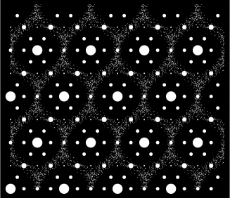
Fig. 3: Diffraction image of the tiling of Fig. 2 with scatterers of equal strength $1$. It was calculated numerically by means of standard FFT, because this is simpler than using the exact expression for the $ac$ part.

We integrate over $v$ for $x<0$; the case of positive $x$ can be treated analogously. The integrand is singular at

$$v_{\pm}=\frac{-\alpha\pm\sqrt{\alpha^{2}-4\beta}}{2(bw+d)}$$ (11)

with $\alpha=(aw+c(w^{2}+1))$ and $\beta=w(bw+d)(b+dw)$, but only $v_{+}$ lies inside the unit circle. Thus,

$$I=2\pi i\int\limits_{S^{1}}\frac{g(p_{1},p_{2},v_{+},w)v_{+}^{-x}w^{-y}}{(v_{+}-v_{-})(bw+d)}dw.$$ (12)

Away from the phase transitions, it can be shown that $|v_{+}|<1$. With $\tilde{v}_{+}=\max_{\varphi_{2}}v_{+}$ we get

$$|I| \leq 2\pi\int_{S^{1}}\frac{|g(p_{1},p_{2},v_{+},w)||v_{+}|^{-x}}{|(v_{+}-v_{-})(bw+d)|}dw$$

$$\leq 2\pi|\tilde{v}_{+}|^{-x}\int_{S^{1}}\frac{|g(p_{1},p_{2},v_{+},w)|}{|(v_{+}-v_{-})(bw+d)|}dw$$

$$=\mathcal{O}\left(e^{-t_{1}|x|}\right),$$ (13)

for some positive constant $t_{1}$, because the remaining integral stays finite. Since the coupling function is invariant under interchange of $x$ and $y$, this can be shown for $y$ as well. As $I$ is maximal for $x=0$ for arbitrary but fixed $y$ and vice versa, we conclude that

$$[x,y]_{p_{1}p_{2}}=\mathcal{O}\left(e^{-(t_{1}|x|+t_{2}|y|)}\right).$$ (14)

The non-constant part of the correlation function in (4.) consists basically of products of $[x,y]$. With such an asymptotic behaviour, one can show that its Fourier transform indeed converges towards a continuous function on $\mathbb{R}^{2}/\Gamma$ (cf [2, Addendum]).

At the Kasteleyn phase transitions, we get crystals consisting only of one rhombus orientation and the corresponding darts (cf [16]). The spectrum thus displays Bragg peaks only. For the Onsager case, we re-substitute $w=e^{-i\varphi_{2}}$ in (12). Because of the symmetry of the kernel, it is sufficient to integrate from $0$ to $\pi$. The kernel reaches its maximum value 1 only at $\varphi_{2}=0$ or $\pi$ and remains smaller elsewhere. Using the same argument as in the treatment of the lozenge tiling in [2], we estimate the kernel by a decreasing/increasing straight line. From the resulting asymptotic behaviour we conclude that the diffuse part of the spectrum is an absolutely continuous measure as well.

5. Acknowledgement

I am grateful to Michael Baake for valuable discussions and to Robert V. Moody and the Dept. of Mathematics, University of Alberta, for hospitality, where part of this work was done.

References

• [1] M. Baake, A guide to mathematical quasicrystals, to appear in: “Quasicrystals”, eds. J.-B. Suck, M. Schreiber, P. Häußler, Springer, Berlin; math-ph/9901014.
• [2] M. Baake and M. Höffe, Diffraction of random tilings: some rigorous results, math-ph/9904005.
• [3] A. Córdoba, Dirac Combs, Lett. Math. Phys. 17 (1989), 191–6.
• [4] J. M. Cowley, Diffraction Physics, 3rd ed., North-Holland, Amsterdam (1995).
• [5] V. Elser, Comments on:“Quasicrystals: A New Class of Ordered Structures”, Phys. Rev. Lett. 54 (1985), 1730.
• [6] A. C. D. van Enter and J. Miȩkisz, How Should One Define a (Weak) Crystal?, J. Stat. Phys. 66 (1992), 1147–53.
• [7] C. Fan and F. Y. Wu, General model of phase transitions, Phys. Rev. B 2 (1970), 723–33.
• [8] M. E. Fisher and J. Stephenson, Statistical mechanics of dimers on a plane lattice. II. Dimer correlations and monomers, Phys. Rev. 132 (1963), 1411–31.
• [9] J. de Gier, Random Tilings and Solvable Lattice Models, PhD-Thesis, Amsterdam (1998).
• [10] C. Henley, Random tilings with quasicrystal order: transfer-matrix approach, J. Phys. A 21 (1988), 1649–77.
• [11] C. Henley, Random Tilings, in: “Quasicrystals: The State of the Art”, ed. D. P. DiVincenzo, P. J. Steinhardt, World Scientific, Singapore (1991), pp. 429–534.
• [12] M. Höffe, Zufallsparkettierungen und Dimermodelle, Diplomarbeit, Tübingen (1997); available from the author.
• [13] D. Joseph, S. Ritsch, C. Beeli, Distinguishing quasiperiodic from random order in high-resolution TEM-images, Phys. Rev. B 55 (1997), 8175–83.
• [14] P. W. Kasteleyn, The statistics of dimers on a lattice, Physica 27 (1961), 1209–25.
• [15] B. McCoy and T. T. Wu, The Two-Dimensional Ising Model, Harvard University Press, Cambridge, MA (1973).
• [16] C. Richard, M. Höffe, J. Hermisson, M. Baake, Random tilings – concepts and examples, J. Phys. A (1998), 6385–408.
• [17] M. Reed and B. Simon, Functional Analysis, 2nd ed., Academic Press, San Diego (1980).
• [18] D. Ruelle, Statistical Mechanics: Rigorous Results, Addison Wesley, Redwood City (1969).