Eigenvalue density for a class of Jacobi matrices




I. V. Krasovsky

Max-Planck-Institut für Physik komplexer Systeme

Nöthnitzer Str. 38, D-01187, Dresden, Germany

E-mail: ivk@mpipks-dresden.mpg.de

and

B.I.Verkin Institute for Low Temperature Physics and Engineering

47 Lenina Ave., Kharkov 310164, Ukraine.

Abstract. We obtain the asymptotic distribution of eigenvalues of real symmetric tridiagonal matrices as their dimension increases to infinity and whose diagonal and off-diagonal elements asymptotically change with the index $n$ as $J_{nt+i\;nt+i}\sim a_{i}\varphi(n)$, $J_{nt+i\;nt+i+1}\sim b_{i}\varphi(n)$, $i=0,1,\dots,t-1$, where $a_{i}$ and $b_{i}$ are finite, and $\varphi(n)$ belongs to a certain class of nondecreasing functions.

A very versatile method for calculation of physical properties of quantum systems ([References–References] and references in [References–References]) uses the Lanczos procedure to reduce the matrix of the Hamiltonian or some other relevant operator to the tridiagonal form. After this reduction, various properties of tridiagonal (Jacobi) matrices provide much help in solving the problem at hand. An important problem arising in connection with this method is to find the asymptotic distribution of eigenvalues of Jacobi matrices (when the dimension of the matrix increases to infinity) if the asymptotics of the matrix elements is known. The purpose of this note is to present a solution to this problem in a particular case.

Let $J$ be a symmetric Jacobi matrix with real matrix elements (that is $J_{ik}=J_{ki}$, $i,k=0,1,2,\dots$, $J_{ik}=0$ if $|i-k|>1$, $J_{i\;i+1}\neq 0$ ). Suppose that $\lim_{n\to\infty}J_{nt+i\;nt+i}/\varphi(n)=a_{i}$ and $\lim_{n\to\infty}J_{nt+i\;nt+i+1}/\varphi(n)=b_{i}$, $i=0,1,\dots,t-1$, where $a_{i},b_{i}<\infty$ are not all simultaneously zero; $t$ is a positive integer; the function $\varphi(x):{\bf R}^{+}\to{\bf R}^{+}$ is nondecreasing and satisfies the condition $\lim_{n\to\infty}\varphi(n+x)/\varphi(n)=1$ for any real $x$. Note that for $\varphi(n)=1$ the matrix $J$ is asymptotically periodic.

Furthermore, let $J(n)=||J_{ik}||_{i,k=0}^{nt-1}$ denote the $nt\times nt$ truncated $J$. Our aim is to calculate the eigenvalue density $\rho(z)$ of $J(n)/\varphi(n)$ as $n\to\infty$. It is defined by the requirement that $\rho(z)dz$ be in the limit $n\to\infty$ the relative number of eigenvalues of $J(n)/\varphi(n)$ in the interval $dz$.

We now impose a further limitation on the form of $\varphi(n)$: suppose that there exists a continuous function defined by $g(\omega)=du/d\omega$, where $\omega(u)=\lim_{n\to\infty}\varphi(nu)/\varphi(n)$ for $u\in[0,1]$. Note that for $\varphi(n)=n^{\gamma}$, $\gamma>0$, we have $g(\omega)=\omega^{-1+1/\gamma}/\gamma$.

The ideas of these definitions come from the works [References,References], where the case $t=1$ was considered, and the moments of the eigenvalue density $\rho(z)$ were calculated. The explicit expression for $\rho(z)$ was given in [References] for $t=1$, $a=0$. It is called Nevai-Ullman distribution. Using a different approach, Van Assche has obtained for $\varphi(n)=n^{\gamma}$, and arbitrary $a$, $b$ the density $\rho(z)$ for $t=1$ [References] and (implicitly) for $t=2$ [References]. We will now obtain $\rho(z)$ for any $t$ and $a$, $b$ by generalizing the method of [References,References].

Before that, let us recall some facts about periodic symmetric Jacobi matrices. Let $L$ be such a matrix defined by the formulas $L_{nt+i\;nt+i}=a_{i}$ and $L_{nt+i\;nt+i+1}=b_{i}$, $i=0,1,\dots,t-1$, $n=0,1,\dots$. The same $a_{i}$, $b_{i}$ appear in our definition of $J$. Define two systems of polynomials $p_{k}(x)$ and $q_{k}(x)$ by the initial conditions $p_{0}=1$, $p_{1}=(x-a_{0})/b_{0}$; $q_{0}=0$, $q_{1}=-b_{t-1}/b_{0}$ and the same (for $y_{k}=p_{k}$ or $y_{k}=q_{k}$) recurrence relation:

$$y_{k+1}=((x-a_{k})y_{k}-b_{k-1}y_{k-1})/b_{k},\qquad k=1,2,\dots,t-1.$$

Let $S(x)=p_{t}(x)+q_{t-1}(x)$. The spectrum of $L$ consists of exactly $t$ bands: the image of $[-2,2]$ under the inverse of the transform $S(x)=\lambda$. The boundaries of the bands (denote them $\mu_{i}$, $\nu_{i}$, $i=1,\dots,t$, $\nu_{0}\equiv-\infty<\mu_{1}\leq\nu_{1}\leq\mu_{2}\leq\nu_{2}\leq\cdots\leq\nu_{t}<\mu_{t+1}\equiv\infty$) are solutions to the equations $S(x)=\pm 2$. Thus, the spectrum of $L$ is ${\rm spec}(L)=\cup_{i=1}^{t}[\mu_{i},\nu_{i}]$. The eigenvalue density of $L$ is given by the formula $\rho_{0}(x)=|dS(x)/dx|/(t\pi\sqrt{4-S(x)^{2}})$, for $x\in{\rm spec}(L)$, and $\rho_{0}(x)=0$ otherwise.

Note that for $t=1$ we have $\rho_{0}(x)=(\pi\sqrt{4b_{0}^{2}-(x-a_{0})^{2}})^{-1}$.

Theorem Let $f(z,\omega)=g(\omega)\rho_{0}(z/\omega)/\omega$. Then, under the conditions specified above, the eigenvalue density of $J(n)/\varphi(n)$ as $n\to\infty$ is the following:

1) $0\in[\mu_{k},\nu_{k}]$ for some $k$ ($1\leq k\leq t$),

$$\rho(z)=\cases{\left[\int_{z/\nu_{i}}^{1}+\sum_{j=i+1}^{t}\int_{z/\nu_{j}}^{z/\mu_{j}}\right]f(z,\omega)d\omega,&$z\in[\mu_{i},\nu_{i}]$, $\mu_{i}\geq 0$\cr{\it the\;preceding\;expression\;with\;\it i=k},&$z\in[0,\nu_{k}]$\cr\left[\sum_{j=i+1}^{t}\int_{z/\nu_{j}}^{z/\mu_{j}}\right]f(z,\omega)d\omega,&$z\in(\nu_{i},\mu_{i+1})$, $\nu_{i}\geq 0$\cr\left[\int_{z/\mu_{i}}^{1}+\sum_{j=1}^{i-1}\int_{z/\mu_{j}}^{z/\nu_{j}}\right]f(z,\omega)d\omega,&$z\in[\mu_{i},\nu_{i}]$, $\nu_{i}\leq 0$\cr{\it the\;preceding\;expression\;with\;\it i=k},&$z\in[\mu_{k},0]$\cr\left[\sum_{j=1}^{i}\int_{z/\mu_{j}}^{z/\nu_{j}}\right]f(z,\omega)d\omega,&$z\in(\nu_{i},\mu_{i+1})$, $\mu_{i+1}\leq 0$};$$

2) $0\in(\nu_{k},\mu_{k+1})$ for some $k$ ($0\leq k\leq t$), The expression for $\rho(z)$ is the same as above (two formulas for $z\in[0,\nu_{k}]$ and $z\in[\mu_{k},0]$ should be dropped) except in the interval $(\nu_{k},\mu_{k+1})$ where

$$\rho(z)=\cases{\left[\sum_{j=k+1}^{t}\int_{z/\nu_{j}}^{z/\mu_{j}}\right]f(z,\omega)d\omega,&$z\in(0,\mu_{k+1})$\cr\left[\sum_{j=1}^{k}\int_{z/\mu_{j}}^{z/\nu_{j}}\right]f(z,\omega)d\omega,&$z\in(\nu_{k},0)$.}$$

Sketch of the proof. Some basic ideas of the proof we borrow from [References,References] where the case $t=1$ was considered. Let us denote $K_{M}=\int_{-\infty}^{\infty}x^{M}\rho_{0}(x)dx$, where $M$ is a nonnegative integer, and verify first the following identity:

$$\lim_{k\to\infty}{1\over t}\sum_{i=0}^{t-1}\left(\left[{J\over\varphi(k)}\right]^{M}e_{kt+i},e_{kt+i}\right)=K_{M},$$ (1)

where $\{e_{j}\}_{j=0}^{\infty}$ is an orthonormal basis in which the above defined matrices of operators $J$ and $L$ are written. Indeed, it is obvious that the l.h.s. of this identity is equal to

$$\lim_{k\to\infty}{1\over t}\sum_{i=0}^{t-1}(L^{M}e_{kt+i},e_{kt+i}),$$

while

$$\lim_{k\to\infty}{1\over t}\sum_{i=0}^{t-1}(L^{M}e_{kt+i},e_{kt+i})=\lim_{n\to\infty}{1\over nt}\sum_{j=0}^{nt-1}(L^{M}e_{j},e_{j})=K_{M}.$$ (2)

From (1) it follows that

$${1\over t}\sum_{k=0}^{n-1}\sum_{i=0}^{t-1}(J^{M}e_{kt+i},e_{kt+i})=\sum_{k=0}^{n-1}\varphi(k)^{M}(K_{M}+\epsilon_{k}),$$ (3)

where $\epsilon_{k}\to 0$ as $k\to\infty$. We have:

$$\lim_{n\to\infty}\frac{\sum_{k=0}^{n-1}\varphi(k)^{M}}{n\int_{0}^{1}\varphi(xn)^{M}dx}=1,\qquad\lim_{n\to\infty}\frac{\sum_{k=0}^{n-1}\epsilon_{k}\varphi(k)^{M}}{\sum_{k=0}^{n-1}\varphi(k)^{M}}=0.$$ (4)

Hence, (3) can be rewritten as follows:

$${1\over t}\sum_{k=0}^{nt-1}(J^{M}e_{k},e_{k})=(K_{M}+\delta_{n})n\int_{0}^{1}\varphi(xn)^{M}dx,$$ (5)

where $\delta_{n}\to 0$ as $n\to\infty$.

To proceed further, we will need to estimate the sum

$$Z_{n}(M)=\sum_{k=0}^{nt-1}(J^{M}e_{k},e_{k})-\sum_{k=1}^{nt}x_{k,n}^{M},$$ (6)

where $x_{k,n}$, $k=1,\dots,nt$ are the eigenvalues of $J(n)$. Note that $Z_{n}(M)$ is the difference between traces of two matrices, one of which is obtained by first taking the power $J^{M}$ and then truncating the result; and the other one, by first truncating $J$ and then taking the power $J(n)^{M}$. It is easy to calculate that for $n$ large enough $Z_{n}(0)=Z_{n}(1)=0$, $Z_{n}(2)=J_{nt\;nt-1}^{2}$, $Z_{n}(3)=J_{nt\;nt-1}^{2}(J_{nt\;nt}+J_{nt-1\;nt-1})$, etc. In general, we have for all sufficiently large $n$:

$$|Z_{n}(M)|\leq f(M)\max_{0\leq i,k\leq n+M}|J_{i\;k}|^{M},$$ (7)

where $f(M)$ does not depend on $n$. In view of this estimate, (5) leads to the identity:

$$\lim_{n\to\infty}\frac{\sum_{k=1}^{nt}x_{k,n}^{M}}{nt\int_{0}^{1}\varphi(xn)^{M}dx}=K_{M}.$$ (8)

Changing the variables $x_{k,n}=\varphi(n)z_{k,n}$ and taking the limit, we have:

$${m_{M}\equiv\lim_{n\to\infty}{1\over nt}\sum_{k=1}^{nt}z_{k,n}^{M}=\int_{0}^{1}\omega^{M}(x)dxK_{M}=\int_{0}^{1}\omega^{M}g(\omega)d\omega\int_{-\infty}^{\infty}x^{M}\rho_{0}(x)dx,}$$

  (9)

where $\omega(x)$ and $g(x)$ are defined as above.

Changing the variables $z=\omega x$, $\psi=\omega$ in the double integral in (9), we get:

$$m_{M}=\int_{-\infty}^{\infty}z^{M}\rho(z)dz,$$ (10)

where $\rho(z)$ is defined in cases 1 and 2 as in Theorem. Since the actual support of integration in (10) is finite, the function $\rho(z)$ is defined uniquely by $m_{M}$, $M=0,1,\dots$. Thus, $\rho(z)$ can be identified with the eigenvalue density.

Although the simple case $t=1$ has appeared to a large extent in the literature, we will now discuss it to give the reader a better feeling of the results and to show the relation to other methods to investigate the distribution of eigenvalues.

So from now on let $t=1$ and define $a_{0}=a$, $b_{0}=b/2$. Henceforth, we put $a\geq 0$ and $b\geq 0$ without loss of generality (it is easily seen that $\rho(z)$ for the pairs $a$, $b$ and $a$, $-b$ is the same). It will be interesting to note the distinction between the cases $a>b$ and $a<b$.

Corollary of the theorem Let $t=1$, $a_{0}=a$, $b_{0}=b/2$. Under the conditions specified above, the eigenvalue density of $J(n)/\varphi(n)$ as $n\to\infty$ is the following:

1) $0\leq a/b\leq 1$,

$\rho(z)=\frac{1}{\pi}\int_{z/(a+b\,{\rm sign}\,z)}^{1}\frac{g(\omega)d\omega}{\sqrt{b^{2}\omega^{2}-(z-a\omega)^{2}}}$ if $z\in[a-b,a+b]$, and $\rho(z)=0$ otherwise;

2) $a/b>1$,

$$\rho(z)=\cases{\frac{1}{\pi}\int_{(a-b)/(a+b)}^{1}\frac{g(\omega\frac{z}{a-b})d\omega}{\sqrt{b^{2}\omega^{2}-(a-b-a\omega)^{2}}},&$z\in[0,a-b]$\cr\frac{1}{\pi}\int_{z/(a+b)}^{1}\frac{g(\omega)d\omega}{\sqrt{b^{2}\omega^{2}-(z-a\omega)^{2}}},&$z\in[a-b,a+b]$\cr 0,&$z\notin[0,a+b]$}.$$

Note that for $\varphi(n)=n^{\gamma}$, $\gamma>0$ we can write case 2 in a simpler form:

$$\rho(z)=\cases{h(a-b)\left(\frac{z}{a-b}\right)^{-1+1/\gamma},&$z\in[0,a-b]$\cr h(z),&$z\in[a-b,a+b]$\cr 0,&$z\notin[0,a+b]$},$$

where

$$h(z)=\frac{1}{\pi\gamma}\int_{z/(a+b)}^{1}\frac{\omega^{-1+1/\gamma}d\omega}{\sqrt{b^{2}\omega^{2}-(z-a\omega)^{2}}}.$$

The form of $\rho(z)$ is illustrated for $\varphi(n)=n^{\gamma}$, in Figures 1,2. When $\gamma\to 0$ the density $\rho(z)$ for all $a,b$ approaches the distribution $\rho_{0}(z)=(\pi\sqrt{b^{2}-(z-a)^{2}})^{-1}$, $z\in[a-b,a+b]$.

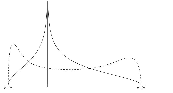
Figure 1: Example of the density of eigenvalues $\rho(z)$ for $a<b$, $\varphi(n)=n^{\gamma}$. Solid curve corresponds to some $\gamma\geq 1$, dashed curve, to $0<\gamma<1$.

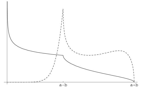
Figure 2: Example of the density of eigenvalues $\rho(z)$ for $a>b$, $\varphi(n)=n^{\gamma}$. Solid curve corresponds to some $\gamma>1$, dashed curve, to $0<\gamma<1$ (in fact, it is obvious from the picture that the second derivative of the dashed curve is positive for $z\in[0,a-b]$, so it corresponds to some $\gamma<1/2$).

One can note that for $\varphi(n)=n$ the matrix $J/r$, where $r=\sqrt{|a^{2}-b^{2}|}$, has the same asymptotics of the matrix elements as the matrix associated with the Meixner (for $a>b$) or Meixner-Pollaczek (for $a<b$) orthogonal polynomials. Asymptotics of the eigenvalues of $J(n)/r$ is the asymptotics of the zeros (to the main order) of these polynomials.

For $\varphi(n)=n$ the function $\rho(z)$ is elementary. Integration gives in cases 1 and 2, respectively

$$1)\quad\rho(z)=\cases{\frac{1}{\pi r}{\rm arccosh}\left|{r^{2}\over zb}+{a\over b}\right|,&$z\in[a-b,a+b]$\cr 0,&$z\notin[a-b,a+b]$};$$

$$2)\quad\rho(z)=\cases{1/r,&$z\in[0,a-b]$\cr\frac{1}{\pi r}{\rm arccos}\left(-{r^{2}\over zb}+{a\over b}\right),&$z\in[a-b,a+b]$\cr 0,&$z\notin[0,a+b]$},$$

$$0\leq\arccos(x)\leq\pi.$$

Replacing $r$ by 1 in these formulas gives the contracted asymptotic densities of zeros of the Meixner-Pollaczek (case 1) and Meixner (case 2) polynomials. The quantities $a$, $b$ are expressed in this case in terms of the parameters of the polynomials. For detailed discussion of zero densities for various systems of orthogonal polynomials see [References] and references therein.

The Meixner and Meixner-Pollaczek polynomials satisfy difference equations of the type [References]:

$$B(x)p_{n}(x+\delta)-C(x,n)p_{n}(x)+D(x)p_{n}(x-\delta)=0.$$ (11)

By analyzing such equations, it is possible to obtain information on the asymptotic distribution of zeros of $p_{n}(x)$ [References]. Thus, corollary of the theorem for $\varphi(n)=n$ can be given an alternative proof, and also more precise information (than the density) about asymptotics of zeros can be found: distribution of zeros of the Meixner polynomials $p_{n}(nz)$ in the region $z\in[0,a-b]$ where $\rho(z)=1$.

Acknowledgements

I thank Alphonse Magnus and Walter Van Assche for useful correspondence.

References

[1]
[2] Peresada V I 1968 Fizika kondensirovannovo sostojanija
(Physics of Condensed Matter) Inst. for Low Temperature
Physics and Engeneering, Kharkov, issue 2, 172 (in Russian)
[3] Peresada V I and Afanas’ev V N 1970 Sov.Phys.JETP31 78 [Zh.Eksp.Teor.Fiz.58 135]
[4] Peresada V I, Afanas’ev V N and Borovickov V S 1975
Fiz.Nizk.Temp.1 461 (in Russian)
[5] Ehrenreich H, Seitz F, Turnbull D (ed) 1980
Solid State Physics vol 35 (N.Y.: Academic)
[6]Pettifor D G and Weaire D L (ed) 1985
The Recursion Method and Its Applications (Berlin: Springer)
[7] Lee M H, Hong J, and Florencio J, Jr. 1987
Phys.Scr.T19 498
[8] Krasovsky I V and Peresada V I 1995 J.Phys:A Math.Gen.28 1493; ibid 1996 29 133
[9]
[10] Nevai P G, Dehesa J S 1979 SIAM J.Math.Anal.10 1184
[11] Ullman J L, 1980 in Approximation Theory III,
ed. E W Cheney, (N.Y.: Academic) p. 889
[12] Van Assche W, 1987 Asymptotics for Orthogonal
Polynomials (Berlin: Springer)
[13] Van Assche W, 1988 J.Approx.Theory52 322
[14] Kuijlaars A B J, Van Assche W, 1997, preprint,
The asymptotic zero distribution of orthogonal polynomials with
varying recurrence coefficients
[15]
[16] Koekoek R, Swarttouw R F 1996 The Askey-scheme of
hypergeometric orthogonal polynomials and its -analogue. Delft University
of Technology.
[17]
[18] Krasovsky I V, Asymptotic distribution of zeros
of polynomials satisfying difference equations, to be published