Fast Blow Up in the (4+1)-dimensional Yang Mills Model and the (2+1)-dimensional $S^{2}$ Sigma Model

Abstract

We study singularity formation in spherically symmetric solitons of the (4+1) dimensional Yang Mills model and the charge two sector of the (2+1) dimensional $S^{2}$ sigma model, also known as ${\mathbb{C}}P^{1}$ wave maps, in the adiabatic limit. These two models are very similar. Studies are performed numerically on radially symmetric solutions using an iterative finite differencing scheme. Predictions for the evolution toward a singularity are made from an effective Lagrangian and confirmed numerically. In both models a characterization of the shape of a time slice $f(r,T)$ with $T$ fixed is provided, and ultimately yields an new approximate solutions to the differential equations that becomes exact in the adiabatic limit.

Mathematics Subject Classification: 35-04, 35L15, 35L70, 35Q51, 35Q60 Physics and Astronomy Classification: 02.30.Jr, 02.60.Cb

1 Introduction

In this paper we study two hyperbolic partial differential equations that develop singularities in finite time.

The Yang Mills model displays fast blow up, and the $S^{2}$ sigma model displays both slow blow up and fast blow up. In slow blow up, all relevant speeds go to zero as the singularity is approached. In fast blow up the relevant speeds do not go to zero as the singularity is approached . The charge 1 sector of the $S^{2}$ sigma model, investigated in [3] and [4], exhibits logarithmic slow blow up. The charge 2 sector of the $S^{2}$ sigma model and the similar charge 1 sector of the Yang Mills (4+1)-dimensional model both exhibit fast blow up.

The Yang Mills Lagrangian in 4 dimensons is a generalization of Maxwell’s equations in a vacuum, and is discussed at length in [1]. We can regard this problem as being that of a motion of a particle, where we wish our particles to have certain internal and external symmmetries, which give rise to the various gemoetrical objects in the problem. The states of our particles are given by gauge potentials or connections, denoted $A$, on ${\mathbb{R}}^{4}$, and we identify ${\mathbb{R}}^{4}$ as ${\mathbb{H}}$, the quarternions, $\vec{x}=x_{1}+x_{2}i+x_{3}j+x_{4}k$. The gauge potentials have values in the Lie albegra of $SU(2)$ which can be viewed as purely imaginary quarternions, $\mbox{Im}({\mathbb{H}})$. The curvature $F_{ij}=\partial_{i}A_{j}-\partial_{j}A_{i}+[A_{i},A_{j}]$, where $[A_{i},A_{j}]=A_{i}A_{j}-A_{j}A_{i}$ is the bracket in the Lie Algebra, gives rise to the potential $V(A)=\langle F,F\rangle$ which is a nonlinear function of $A$. The static action is:

$$L=\frac{1}{2}\int\ \langle F_{ij},F_{ij}\rangle d^{4}\vec{x}.$$ (1)

The local minima of (1) are the instantons on 4 dimensional space. These correspond to solutions of Maxwell’s equations in the vacuum. We now consider the wave equation generated by this potential with Lagrangian:

$$L=\frac{1}{2}\int\langle\partial_{t}{A_{i}},\partial_{t}{A_{i}}\rangle-\frac{1}{2}\langle F_{ij},F_{ij}\rangle d^{4}\vec{x}.$$ (2)

Via the calculus of variations, the evolution equation for this (4+1)-dimensional model is

$$\partial_{t}^{2}{A_{i}}=-\raisebox{2.15277pt}{$\bigtriangledown$}_{j}F_{ij}.$$ (3)

Theoretical work on the validity of the geodesic or adiabatic limit approximation for the monopole soltions to the Yang-Mills-Higgs theory on Minkowski space is presented in [8].

The two-dimensional $S^{2}$ sigma model, especially the charge 1 sector, has been studied extensively over the past few years in [2], [5], [6],[7], [9], [10]. It is a good toy model for studying two-dimensional analogues of elementary particles in the framework of classical field theory. Elementary particles are thereby described by classical extended solutions of this model, called solitons. This model is extended to (2+1) dimensions. The previous solitons are static or time-independent solutions, and the dynamics of these solitons are studied. The charge 2 sector of this model is held by general wisdom to be similar to the (4+1)-dimensional Yang Mills model.

The $S^{2}$ sigma model can also be regarded as the continuum limit of an array of Heisensberg ferromagnets.

The static Lagrangian density for the $S^{2}$ sigma model is given by

$$L=\int|\raisebox{2.15277pt}{$\bigtriangledown$}\vec{\phi}|^{2},$$

where $\vec{\phi}$ is a unit vector field.

In the dynamic version of this problem, where $\phi:{\mathbb{R}}^{2+1}\rightarrow S^{2}$, the Lagrangian is

$$L=\int_{{\mathbb{R}}^{2}}|\partial_{t}{\vec{\phi}}|^{2}-|\raisebox{2.15277pt}{$\bigtriangledown$}\vec{\phi}|^{2}.$$

Identifying $S^{2}={\mathbb{C}}P^{1}={\mathbb{C}}\cup\{\infty\}$ we can rewrite this as

$$L=\int_{{\mathbb{R}}^{2}}\frac{|\partial_{t}{u}|^{2}}{(1+|u|^{2})^{2}}-\frac{|\raisebox{2.15277pt}{$\bigtriangledown$}u|^{2}}{(1+|u|^{2})^{2}}.$$ (4)

The calculus of variations on this Lagrangian yields the following equation of motion for the $S^{2}$ sigma model:

$$(1+|u|^{2})(\partial_{t}^{2}u-\partial_{x}^{2}u-\partial_{y}^{2}u)=2\bar{u}(|\partial_{t}u|^{2}-|\partial_{x}u|^{2}-|\partial_{y}u|^{2}).$$ (5)

Here $\bar{u}$ represents the complex conjugate of $u$.

In this paper we first investigate the charge 1 sector of the (4+1)-dimensional Yang Mills model and then in the second part go on to the charge 2 sector of the $S^{2}$ sigma model. In each part, we first derive the evolution equation for our model. Second, we explain the numerical scheme used to investigate it. Third we go over the predictions made by the geodesic approximation for the model. Fourth, we go over the results generated from the computer runs. In both models the results encompass comparing the trajectory of the evolution to that predicted by the geodesic approximation, and characterizing the profile generated at fixed time slices. In both models our investigation of the profiles yields an improvement in approximate solutions of the differential equations, and these approximate solutions become exact in the adiabatic limit.

2 The (4+1)-dimensional Yang Mills Model, Charge 1 Sector

The first things to identify in this problem are the static solutions to equation (3). These are simply the 4 dimensional instantons investigated in [1]. In [1] the form of all such instantons in the degree one sector is shown to be:

$$A(x)=\frac{1}{2}\left\{\frac{(\bar{x}-\bar{a})dx-d\bar{x}(x-a)}{\lambda^{2}+|x-a|^{2}}\right\}\qquad x=x_{1}+x_{2}i+x_{3}j+x_{4}k\in{\mathbb{H}}.$$

The curvature $F$ of this potential is computed by $F=dA+[A,A]$ and is:

$$F=\frac{d\bar{x}\wedge dx}{(\lambda^{2}+|x-a|^{2})^{2}}.$$

One notices the denominators are radially symmetric about $x=a$.

An instanton of unit size centered at the origin would be

$$A(x)=\frac{1}{2}\left\{\frac{\bar{x}dx-d\bar{x}x}{1+|x|^{2}}.\right\}$$

One motion one can study from these static instantons would be to consider connections the form

$$A(r,t)=\frac{1}{2}\left\{\frac{\bar{x}dx-d\bar{x}x}{f(r,t)+r^{2}}\right\}\qquad r=\sqrt{x_{1}^{2}+x_{2}^{2}+x_{3}^{2}+x_{4}^{2}}$$

and derive an equation of motion for $f(r,t)$ from (3). This is actually quite computationally extensive.

To get at this, start with connections of the form

$$A(r,t)=\frac{1}{2}g(r,t)\left\{\bar{x}dx-d\bar{x}x\right\}.$$

Using the formula for $F$ given by $F=dA+[A,A]$, and a symbolic algebra program such as Maple, one can use (3) to calculate the differential equation for $g$:

$$\partial_{t}^{2}{g}=12g^{2}+\frac{5\partial_{r}g}{r}+\partial^{2}_{r}g-8g^{3}r^{2}.$$ (6)

It is much less difficult to now compute a differential equation for $f(r,t)$ if

$$g(r,t)=\frac{1}{f(r,t)+r^{2}}.$$

It is

$$\partial^{2}_{t}f=\partial^{2}_{r}f+\frac{5\partial_{r}f}{r}-\frac{8\partial_{r}fr}{f+r^{2}}+\frac{2}{f+r^{2}}\left((\partial_{t}f)^{2}-(\partial_{r}f)^{2}\right).$$ (7)

The static solutions for $f(r,t)$ are simply horizontal lines, $f(r,t)=c$. The geodesic approximation for motion under small velocities states that solutions should progress from line to line, i.e.,  $f(r,t)=c(t)$. Here the length scale is given by $\sqrt{c}$. $f(r,t)=0$ is a singularity of the system, where the instantons are not well defined. We observe progression from $f(r,t)=c_{0}>0$ towards this singularity. The validity of the geodesic approximation can be evaluated from how $f(0,t)$ evolves versus how it is predicted to evolve, and the differences between $f(r,T)$ with $T$ fixed and a horizontal line.

2.1 Numerics for the (4+1)-dimensional Yang Mills Model

In both the (4+1)-dimensional Yang Mills Model and the $S^{2}$ sigma model covered in section 3, a finite difference method is used to compute the evolution of (7) and (12) numerically. Unless otherwise noted, centered differences are used consistently, so that

$$\partial_{r}g(x) \approx \frac{g(x+\delta)-g(x-\delta)}{2\delta}$$

$$\partial_{r}^{2}g(x) \approx \frac{g(x+\delta)+g(x-\delta)-2g(x)}{\delta^{2}}.$$

In order to avoid serious instabilities in (7), the terms

$$\partial^{2}_{r}f+\frac{5\partial_{r}f}{r}$$ (8)

must be modeled in a special way. We see this revisited for the $S^{2}$ sigma model in section 3. Allow

$$\partial^{2}_{r}f+\frac{5\partial_{r}f}{r}=\mathcal{L}f$$

where

$$\mathcal{L}=r^{-5}\partial_{r}r^{5}\partial_{r}.$$

This operator has negative real spectrum, hence it is stable. However the naive central differencing scheme on (8) always results in uncontrolled growth near the origin. General wisdom holds that when one has difficulties with the numerics in one part of a problem one should find a differencing scheme for that specific part in the natural to that specific part. Applying this allowed for the removal of the problem near the origin. Instead of using centered differences on $\partial^{2}_{r}f$ and on $\partial_{r}f$, we difference the operator:

$$\mathcal{L}f=r^{-5}\partial_{r}r^{5}\partial_{r}.$$

The “natural differencing scheme” is then

$$\mathcal{L}f\approx r^{-5}\left[\frac{\left(r+\displaystyle{\frac{\delta}{2}}\right)^{5}\left(\displaystyle{\frac{f(r+\delta)-f(r)}{\delta}}\right)-\left(r-\displaystyle{\frac{\delta}{2}}\right)^{5}\left(\displaystyle{\frac{f(r)-f(r-\delta)}{\delta}}\right)}{\delta}\right].$$

In [6], studying the charge 1 sector of the $S^{2}$ sigma model, stationary solutions were found to be unstable and to shrink spontaneously under the numerical scheme. This model exhibits no such difficulties. Unless bumped from the stationary state with an initial velocity, stationary solutions do not evolve in time.

A discussion of the stability of this numerical scheme is available in [3].

With the differencing explained, to derive $f(r,t+\triangle t)$, one always has a guess for $f(r,t+\triangle t)$ given by either the initial velocity, e.g. $f(r,t+\triangle t)=f(r,t)+v_{0}\triangle t$, or by $f(r,t+\triangle t)=2f(r,t)-f(r,t-\triangle t)$. Use this to compute $\partial_{t}{f}(r,t)$ on the right hand side of (7). Then solve for $f(r,t+\triangle t)$ in the difference for $\partial^{2}_{t}f(r,t)$, and iterate this procedure to get a more precise answer. So, one iterates

$$f(r,t+\triangle t) = 2f(r,t)-f(r,t-\triangle t)+(\triangle t)^{2}\left[\partial^{2}_{r}f(r,t)-\frac{5\partial_{r}f(r,t)}{r}\right.$$

$$-\left.\frac{2\partial_{t}{f}(r,t)^{2}}{f(r,t)+r^{2}}-\frac{2\partial_{r}f(r,t)^{2}}{f(r,t)+r^{2}}-\frac{8\partial_{r}f(r,t)r}{f(r,t)+r^{2}}\right],$$

where all derivatives on the right hand side are represented by the appropriate differences.

There remains the question of the boundary conditions. The function $f$ is only modeled out to a value $r=R\gg 0$. Initial data for $f(r,0)$ was originally a horizontal line. The corresponding boundary conditions are that $f(R,t)=f(R-\triangle r,t)$, and that

$$f(0,t)=\frac{4}{3}f(\triangle r,t)-\frac{1}{3}f(2\triangle r,t)$$

i.e.,  that $f$ is an even function.

Subsequent investigation of the model indicated that the appropriate form for $f(r,t)$ was a parabola instead of a line, and the $f(R,t)$ boundary condition was changed to reflect this. For the runs with parabolic initial data, we set the boundary condition at $R$ to be:

$$\partial_{r}f(R,t)=\partial_{r}f(R-\triangle r,t)\frac{R}{R-\triangle r}.$$

2.2 Predictions of the Geodesic Approximation for the (4+1)-dimensional Yang Mills Model

Equation (2) gives us the Lagrangian for the general version of this problem. We are using

$$A=\frac{1}{2}\left\{\frac{\bar{x}dx-d\bar{x}x}{f+r^{2}}\right\}\qquad r=\sqrt{x_{1}^{2}+x_{2}^{2}+x_{3}^{2}+x_{4}^{2}},$$

and we use the geodesic approximation which predicts we move close to the moduli space of these solutions. Restricting the Lagrangian to this moduli space gives us an effective Lagrangian. The portion of the integral given by

$$-\frac{1}{4}\int_{{\mathbb{R}}^{4}}\langle F_{ij},F_{ij}\rangle d\vec{x}$$

represents the potential energy and integrates to a topological constant, hence it may be ignored. We see this same phenomenon again in section 3.2 in the study of the $S^{2}$ sigma model. We need to calculate

$$\frac{1}{2}\int_{{\mathbb{R}}^{4}}\langle\partial_{t}{A_{i}},\partial_{t}{A_{i}}\rangle d\vec{x}.$$

First calculate

$$\langle\partial_{t}{A_{i}},\partial_{t}{A_{i}}\rangle=\frac{3r^{2}(\partial_{t}f)^{2}}{(f+r^{2})^{4}}.$$

So the Lagrangian is

$$\int_{{\mathbb{R}}^{4}}\frac{3r^{2}(\partial_{t}f)^{2}}{(f+r^{2})^{4}}d\vec{x},$$

If we take $f=\mbox{constant}$, using $\vec{y}=\vec{x}/\sqrt{f}$ we can rewrite this integral as

$$\frac{3(\partial_{t}f)^{2}}{f}\int_{{\mathbb{R}}^{4}}\frac{|y|^{2}}{(1+|y|^{2})^{4}}d\vec{y}.$$

The integral with respect to $\vec{y}$ converges, hence we have the effective Lagrangian

$$L=c\frac{(\partial_{t}f)^{2}}{f}.$$

This is purely kinetic energy. Since the potential energy is constant, so is the kinetic energy. We have

$$\frac{(\partial_{t}f)^{2}}{f}=k.$$

Integrating this we get

$$f=(c_{1}t+c_{2})^{2}.$$

If $f=0$ occurs at time $T$, we find

$$T=-\frac{c_{2}}{c_{1}}$$

hence we rewrite this as

$$f=a(t-T)^{2}.$$

This is how we predict that $f(0,t)$ will evolve. This same evolution is predicted in section 3.2.

2.3 Results for the (4+1)-Dimensional Yang Mills Model, Evolution of $f(0,t)$

The computer model was run under the condition that $f(r,0)=f_{0}$ with various small velocities. The initial velocity is $\partial_{t}{f}(r,0)=v_{0}$, other input parameters are $R=r_{max}$, $\triangle r$ and $\triangle t$.

The first question to ask is how does the evolution of the origin occur. We note that as $r\rightarrow\infty$ equation (7) becomes the regular linear wave equation

$$\partial^{2}_{t}f=\partial^{2}_{r}f,$$

and so the interesting nonlinear behavior is at the origin. Consequently we track the evolution of $f(0,t)$.

We find that the evolution of $f(0,t)$ evolves exactly as predicted, as a parabola of the form:

$$f(0,t)=a(t-T)^{2}.$$

Unsurprisingly, we obtain this same result in section 3.3 for the $S^{2}$ sigma model.

The time to “blow up” is the parameter $T$ in this equation. Recall that $f_{0}=f(r,0)$ is the initial height and $\partial_{t}{f}_{0}(r,0)=v_{0}$ is the initial velocity. Using a least squares parabolic fit to the origin data obtained after $f(0,t)\leq 0.5f_{0}$, one obtains the parameters $a$ and $T$ for a given origin curve. Table 1 shows the behavior.

Table 1: Parabolic fit to $f(0,t)$ vs. Initial conditions $f_{0}$ and $v_{0}$

$$\begin{array}[]{*{4}{r}}f_{0}&v_{0}&a&T\\ 1.0&-0.010&0.00002501&200.1\\ 2.0&-0.010&0.00001257&399.4\\ 0.5&-0.010&0.00005166&99.0\\ 4.0&-0.010&0.00000626&799.7\\ 4.0&-0.020&0.00002503&400.1\\ 4.0&-0.005&0.00000157&1599.3\end{array}$$

We calculate the parameters $a$ and $T$ from the initial conditions, and we find

$$a=\frac{v_{0}^{2}}{4f_{0}},$$

and

$$T=\frac{2f_{0}}{|v_{0}|}.$$

A typical evolution of $f(0,t)$ is given in Figure 1. In this figure, the equation $0.000025(t-200)^{2}$ neatly overlays the graph of $f(0,t)$. This picture represents the evolution where $f_{0}=1.0$ and $v_{0}=-0.01$. Hence $a=\frac{(0.01)^{2}}{4(1.0)}=0.000025$ and $T=\frac{2(1.0)}{0.01}=200,$ as predicted.

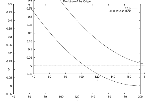
Figure 1: Evolution $f(0,t)$.

2.4 Characterization of Time Slices $f(r,T)$: Evolution of a Horizontal Line in the (4+1)-dimensional Yang Mills Model

The most striking immediate result is that the initial line, $f(r,0)=f_{0},$ evolved an elliptical bump at the origin that grew as time passed. This happens again in section 3.4 with the $S^{2}$ sigma model. Figure 2 shows this behavior.

Figure 2: (4+1)-dimensional Yang Mills model, Time Slices $f(r,T)$ evolve an elliptical bump at the origin

The elliptical bumps can be modeled as

$$\frac{x^{2}}{a^{2}}+\frac{(y-k)^{2}}{b^{2}}=1.$$ (9)

The question naturally arises as to how the parameters $a$, $b$ and $k$ evolve. This is straightforward:

$$a=t$$

$$b=\frac{v_{0}^{2}}{4f_{0}}t^{2}$$

$$k=f_{0}+v_{0}t$$

2.5 Characterization of Time Slices $f(r,T)$: Evolution of a Parabola in the (4+1)-dimensional Yang Mills Model

The elliptical bump that formed in the evolution of a horizontal line and the various configurations that ensued after it bounced off the $r=0$ and $r=R$ boundary suggested that perhaps the curve was trying to obtain the shape of a parabola. After all, near $r=0$, ellipses are excellent approximations for parabolas of the form

$$f(r,t)=pr^{2}+h.$$ (10)

To get the parabola, calculate from the general form of our ellipse in (9)

$$\frac{dy}{dx}=-\frac{x^{2}b^{2}}{(y-k)a^{2}}$$

so

$$\frac{d^{2}y}{dx}=\frac{-b^{2}}{(y-k)a^{2}}-\frac{xb^{2}}{(y-k)^{2}a^{2}}\frac{dy}{dx}$$

At $x=0$, $y-k=b$ and this gives

$$\frac{d^{2}y}{dx}=\frac{-b}{a^{2}}.$$

Recall from the previous section that $b=ct^{2}$ and $a=t$, so this gives

$$\frac{d^{2}y}{dx^{2}}=-c.$$

The identification of $c$ gives

$$\frac{d^{2}y}{dx^{2}}=-\frac{v_{0}^{2}}{4f_{0}}.$$

So

$$p=-\frac{1}{2}\frac{d^{2}y}{dx^{2}}=-\frac{v_{0}^{2}}{8f_{0}}$$

When a run is started with this initial data, $\partial_{t}{f_{0}}=v_{0}=-0.01$, $f_{0}=f(0,0)=1.0$ and $p=-\frac{v_{0}^{2}}{8f_{0}}=-0.0000125$, the time slices of the data have this same profile. This is shown in figure 3.

Figure 3: (4+1)-dimensional Yang Mills model: Time slices of the evolution of a parabola are parabolas.

The curvature of the parabola at the origin, as measured by the parameter $p$ from equation (10) changes by less than 1 part in 100 during the course of this evolution, a graph of $p$ over time can be seen in figure 4.

Figure 4: (4+1)-dimensional Yang Mills model: evolution of parabolic parameter $p$ with time.

The other parameter in equation (10) for the parabola, $h$, should be given by the height of the origin, but this was calculated in the previous section to be $a(t-T)^{2}$, substituting the expressions for $c$ and $T$ we obtain:

$$h(t)=\frac{v_{0}^{2}}{4f_{0}}\left(t-\frac{2f_{0}}{|v_{0}|}\right)^{2}.$$

This is indeed the correct form, as shown in figure 5. The initial conditions were $v_{0}=-0.01$ and $f_{0}=f(0,0)=1.0$, hence $h(t)=0.000025(t-200)^{2}$. The plot of the function overlays the data.

Figure 5: (4+1)-dimensional Yang Mills model: Parabolic parameter $h$ as a function of time evolves as $f(0,t)$.

Now, using both expressions for $p$ and $h$, one can get the general form of a parabolic $f(r,t)$, which is

$$f(r,t)=\frac{v_{0}^{2}}{8f_{0}}r^{2}+\frac{v_{0}^{2}}{4f_{0}}\left(t-\frac{2f_{0}}{|v_{0}|}\right)^{2}$$ (11)

Substitute this into the partial differential equation (7), get a common denominator and simplify to obtain:

$$\frac{v_{0}^{2}}{4f_{0}}\left[-\frac{v_{0}^{2}}{4f_{0}}r^{2}+2\frac{v_{0}^{2}}{4f_{0}}\left(t-\frac{2f_{0}}{|v_{0}|}\right)^{2}+2r^{2}\right]\stackrel{{\scriptstyle?}}{{=}}$$

$$\frac{v_{0}^{2}}{4f_{0}}\left[\frac{v_{0}^{2}}{4f_{0}}r^{2}+2\frac{v_{0}^{2}}{4f_{0}}\left(t-\frac{2f_{0}}{|v_{0}|}\right)^{2}+2r^{2}\right].$$

Clearly these two sides are not the same, and the difference between them is

$$2\left(\frac{v_{0}^{2}}{4f_{0}}\right)^{2}r^{2}.$$

Since our concern is the adiabatic limit, $v_{0}^{2}/(f_{0})$ is always chosen to be small, and this difference goes to zero in the adiabatic limit. This term is always much smaller than the $2r^{2}$ term, and since we only have accurate numerics away from the neighborhood of the singularity, the term with $t-2f_{0}/|v_{0}|$ is on the order of magnitude $f_{0}/|v_{0}|$, which is large compared to the correction. This provides an improved approximate solution for this model which becomes exact in the adiabatic limit. This same behavior is found in section 3.5

The form of the connection $A$ given by this parabolic model is

$$A(r,t)=\frac{1}{2}\left\{\frac{\bar{x}dx-d\bar{x}x}{\left(1-\frac{v_{0}^{2}}{8f_{0}}\right)r^{2}+\frac{v_{0}^{2}}{4f_{0}}\left(t-\frac{2f_{0}}{|v_{0}|}\right)^{2}}\right\}.$$

This is close to the connection $A$ given by the geodesic approximation multiplied by an overall factor. This form suggests a relativistic correction.

3 The Charge 2 Sector of the $S^{2}$ Sigma Model

The first thing to identify in this problem are the static solutions determined by equation (5). These are outlined in [9] among others. The entire space of static solutions can be broken into finite dimensional manifolds $\mathcal{M}_{n}$ consisting of the harmonic maps of degree $n$. If $n$ is a positive integer, then $\mathcal{M}_{n}$ consists of the set of all rational functions of $z=x+iy$ of degree $n$. We restrict our attention to $\mathcal{M}_{2}$, the charge two sector, on which a generic solution has the form

$$u=\alpha+\frac{\beta z+\gamma}{z^{2}+\delta z+\epsilon}$$

depending on the five complex parameters $\alpha,\beta,\gamma,\delta,\epsilon$. To simplify consider only solutions of the form

$$\frac{\gamma}{z^{2}}$$

with $\gamma$ real. The geodesic approximation predicts that solutions evolve close to

$$\frac{\gamma(t)}{z^{2}}.$$

In this investigation, we use a radially symmetric function $f(r,t)=\gamma$, and calculate the evolution equation for $f(r,t)$. It is:

$$\partial^{2}_{t}f=\partial^{2}_{r}f+\frac{5\partial_{r}f}{r}-\frac{8r^{3}\partial_{r}f}{f^{2}+r^{4}}+\frac{2f}{f^{2}+r^{4}}\left((\partial_{t}f)^{2}-(\partial_{r}f)^{2}\right).$$ (12)

We can evaluate the validity of the geodesic approxmation by evaluating how $f(0,t)$ evolves versus the predicted evolution and how $f(r,T)$ with $T$ fixed varies from being a horizontal line.

Immediate similarities can be seen between (12) and equation (7). The static solutions are $f(r,T)=c$ for $T$ fixed and any constant c. Here the length scale is given by $\sqrt{c}$. We investigate progression from $f(r,0)=c_{0}>0$ towards the singularity at $f(r,T)=0$.

3.1 Numerics for the $S^{2}$ Sigma Model Charge 2 Sector

As with the other models, a finite difference method is used to compute the evolution of (12) numerically. Centered differences are used consistently except for

$$\partial^{2}_{r}f+\frac{5\partial_{r}f}{r}.$$

A naive central differencing scheme here yields serious instabilities at the origin. Similar to what we did in section 2.1, let

$$\mathcal{L}f=r^{-5}\partial_{r}r^{5}\partial rf=\partial^{2}_{r}f+\frac{5\partial_{r}f}{r}.$$

This operator has negative real spectrum, hence it is stable. The natural differencing scheme for this operator is

$$\mathcal{L}f\approx r^{-5}\left[\frac{\left(r+\displaystyle{\frac{\delta}{2}}\right)^{5}\left(\displaystyle{\frac{f(r+\delta)-f(r)}{\delta}}\right)-\left(r-\displaystyle{\frac{\delta}{2}}\right)^{5}\left(\displaystyle{\frac{f(r)-f(r-\delta)}{\delta}}\right)}{\delta}\right].$$

This is the differencing scheme used for these terms.

In [6] studying the charge 1 sector of the $S^{2}$ sigma model it was found that under their numerical procedure stationary solutions were unstable and would evolve in time. This model has no such problems with the stationary solutions. They do not evolve in time unless first bumped with an initial velocity.

Now with the differencing explained, we derive $f(r,t+\triangle t)$ in exactly the same manner as for the (4+1)-dimensional model in section 2.1 and the charge 1 sector in [4]. We have an initial guess for $f(r,t+\triangle t)$, either given by $f(r,t+\triangle t)=f(r,t)+v_{0}\triangle t$ with $v_{0}$ the initial velocity given in the problem, or on subsequent time steps $f(r,t+\triangle t)=2f(r,t)-f(r,t-\triangle t)$. We use this guess to compute $\partial_{t}f(r,t)$ on the right hand side of (12), and then we can solve for a new and improved $f(r,t+\triangle t)$ on the left hand side of (12). Iterate this procedure to get increasingly accurate values of $f(r,t)$.

The boundary condition at the origin is found by requiring that $f(r,t)$ is an even function, hence

$$f(0,t)=\frac{4}{3}f(\triangle r,t)-\frac{1}{3}f(2\triangle r,t).$$

At the $r=R$ boundary the function should be horizontal so $f(R,t)=f(R-\triangle r,t)$.

Subsequent investigation of this model indicated that the appropriate form of $f(r,t)$ was a parabola instead of a line, and in order to investigate this phenomenon, the $f(R,t)$ boundary condition was changed to reflect this. For the runs with parabolic initial data, we set the boundary condition at $R$ to be:

$$\partial_{r}f(R,t)=\partial_{r}f(R-\triangle r,t)\frac{R}{R-\triangle r}.$$

3.2 Predictions of the Geodesic Approximation for the $S^{2}$ Sigma Model

Equation (4) gives us the Lagrangian for the general version of this problem. We are using

$$u=\frac{\lambda}{z^{2}}$$

for our evolution, and via the geodesic approximation we restrict the Lagrangian integral to this space, to give an effective Lagrangian, as we did in section 2.2. The integral of the spatial derivatives of $u$ gives a constant, and hence can be ignored. Under these assumptions, up to a multiplicative constant, the effective Lagrangian becomes

$$L=\int_{0}^{\infty}rdr\frac{r^{4}(\partial_{t}\lambda)^{2}}{\left(r^{4}+\lambda^{2}\right)^{2}}$$

which integrates to

$$L=\frac{(\partial_{t}\lambda)^{2}\pi}{8\lambda}.$$

Since the potential energy is constant, so is the kinetic energy, hence

$$\partial_{t}\lambda=k\sqrt{\lambda}.$$

Integrating this one obtains

$$\lambda=(c_{1}t+c_{2})^{2}.$$

If $\lambda=0$ occurs at time $T$, we find

$$T=-\frac{c_{2}}{c_{1}},$$

hence we rewrite this as

$$\lambda(t)=a(t-T)^{2}.$$

This is exactly the same as the evolution predicted in section 2.2 for the Yang Mills Lagrangian. Since equation (12) tends towards the linear wave equation when $r\rightarrow\infty$, the interesting behavior occurs at the origin. This is how we predict that $f(0,t)$ will evolve.

3.3 Results for the $S^{2}$ Sigma Model: Evolution of $f(0,t)$

The computer model was run under the condition that $f(r,0)=f_{0}$ with various small velocities. The initial velocity is $\partial_{t}{f}(r,0)=v_{0}$, other input parameters are $r_{max}=R$, $\triangle r$ and $\triangle t$.

A typical evolution of $f(0,t)$ is given in Figure 6. This is best modeled by a parabola of the form $a(t-T)^{2}$, exactly as predicted. This curve in particular is approximated by $0.0000998(t-100.)^{2}$.

Figure 6: $S^{2}$ sigma model: Evolution of $f(0,t)$ and overlaying fit to parabola.

We fit $f(0,t)$ to a parabola of the form $a(t-T)^{2}$ for various initial conditions. Table 2 gives initial conditions $f_{0}=f(r,0)$ and $v_{0}=\partial_{t}{f}(r,0)$ and the subsequent $T$ and $a$ when $\triangle r=0.025$ and $\triangle t=0.001$.

Exactly as in section 2.3, we have

$$T = \frac{2f_{0}}{|v_{0}|}$$

and

$$a = \frac{v_{0}^{2}}{4f_{0}}.$$

Table 2: $S^{2}$ sigma model: Parameters for best fit parabola to $f(0,t)$ vs. initial data $f_{0}$ and $v_{0}$.

$$\begin{array}[]{*{3}{r}{l}}f_{0}&v_{0}&\ \ \ T&a\\ 1.0&-0.01&200&0.0000250\\ 1.0&-0.02&100&0.0000998\\ 1.0&-0.03&67&0.000224\\ 1.0&-0.04&50&0.000398\\ 0.5&-0.01&100&0.0000499\\ 2.0&-0.01&400&0.0000125\\ 3.0&-0.01&600&0.00000833\\ \end{array}$$

3.4 Characterization of Time Slices $f(r,T)$: Evolution of a Horizontal Line in the $S^{2}$ Sigma Model

With the evolution of $f(0,t)$ taken care of, we consider the shape of the time slices $f(r,T)$ for a given fixed $T$. As in section 2.4 with the (4+1)-dimensional Yang Mills model, this is rather striking. An elliptical bump forms at the origin, as seen in figure 7.

Figure 7: $S^{2}$ sigma model: Time slices of $f(r,T)$ evolve an elliptical bump at the origin.

Once again exactly as in section 2.4 with the (4+1)-dimensional model, this elliptical bump has equation

$$\frac{x^{2}}{a^{2}}+\frac{(y-k)^{2}}{b^{2}}=1.$$ (13)

The question naturally arises how the parameters $a$, $b$, and $k$ evolve, and as in section 2.4, we once again have

$$a = t$$

$$b = \frac{v_{0}^{2}}{4f_{0}}t^{2}$$

$$k = f_{0}+v_{0}t$$

Close to the origin the ellipse is well approximated by a horizontal line, giving further credence to the validity of the geodesic approximation.

3.5 Characterization of Time Slices $f(r,T)$: Evolution of a Parabola in the $S^{2}$ Sigma Model

As with the (4+1)-dimensional model in section 2.5, the evolution of the ellipse suggested the curve was trying to obtain the shape of a parabola of the form

$$f(r,t)=pr^{2}+h.$$ (14)

To get the general form of the parabola, we follow the calculation from the (4+1)-dimensional model in section 2.5. From our ellipse equation (13):

$$\frac{dy}{dx}=-\frac{x^{2}b^{2}}{(y-k)a^{2}}$$

so

$$\frac{d^{2}y}{dx}=\frac{-b^{2}}{(y-k)a^{2}}-\frac{xb^{2}}{(y-k)^{2}a^{2}}\frac{dy}{dx}$$

At $x=0$, $y-k=b$ and this gives

$$\frac{d^{2}y}{dx}=\frac{-b}{a^{2}}.$$

Recall from the previous section that $b=ct^{2}$ and $a=t$, so this gives

$$\frac{d^{2}y}{dx^{2}}=-c.$$

The identification of $c$ gives

$$\frac{d^{2}y}{dx^{2}}=-\frac{v_{0}^{2}}{4f_{0}}.$$

So

$$p=-\frac{1}{2}\frac{d^{2}y}{dx^{2}}=-\frac{v_{0}^{2}}{8f_{0}}.$$

Rather unsurprisingly, this echoes the result of section 2.5.

When a run is started with this initial data, $\partial_{t}{f_{0}}=v_{0}=-0.02$, $f_{0}=f(0,0)=1.0$ and $p=-\frac{v_{0}^{2}}{8f_{0}}=-0.00005$, the time slices of the data have this same profile. This is shown in figure 8. The parabolic parameter $p$ varies by less than 1 part in 10 during the run as seen in figure 9. The parabolic parameter $h$ evolves close to $f(0,t)$ as seen in figure 10.

Figure 8: $S^{2}$ sigma model: Time slices of the evolution of a parabola are parabolas.

Figure 9: $S^{2}$ sigma model: Evolution of parabolic parameter $p$ with time.

Figure 10: $S^{2}$ sigma model: Evolution of parabolic parameter $h$ with time, comparison to $f(0,t)$.

For a parabola of the form

$$f(r,t)=p(t)r^{2}+h(t),$$

we have

$$p(t)=-\frac{v_{0}^{2}}{8f_{0}},$$

i.e.  $p(t)$ is constant, and

$$h(t)=\frac{v_{0}^{2}}{4f_{0}}\left(t-\frac{2f_{0}}{|v_{0}|}\right).$$

Using the identification of $p$ and $h$ in the parabolic form of $f(r,t)$ and letting

$$\tau=t-\frac{2f_{0}}{|v_{0}|}$$

we have

$$f(r,t)=-\frac{v_{0}^{2}}{8f_{0}}r^{2}+\frac{v_{0}^{2}}{4f_{0}}\tau^{2}.$$

Substitute this into the partial differential equation (12), get a common denominator, and simplify to obtain

$$\frac{v_{0}^{6}}{32f_{0}^{3}}\left(\frac{r^{4}}{4}-r^{2}\tau^{2}+\tau^{4}\right)+\frac{v_{0}^{2}}{2f_{0}}r^{4}\stackrel{{\scriptstyle?}}{{=}}$$

$$-\frac{v_{0}^{6}}{32f_{0}^{3}}\frac{r^{4}}{4}+\frac{v_{0}^{6}}{32f_{0}^{3}}\tau^{4}+\frac{v_{0}^{2}}{2f_{0}}r^{4}.$$

The difference between the two sides is

$$\frac{v_{0}^{6}}{64f_{0}^{3}}r^{4}-\frac{v_{0}^{6}}{32f_{0}^{3}}r^{2}\tau^{2}.$$

As in section 2.5 for the (4+1)-dimensional Yang Mills model, our concern is with the geodesic approximation, and so $v_{0}^{2}/(f_{0})$ is always chosen to be small. The correction is then much smaller than the term

$$\frac{v_{0}^{2}}{2f_{0}}r^{4}.$$

4 Conclusions

The formation of singularities in the geodesic approximation to the (4+1)-dimensional Yang Mills model and the (2+1)-dimensional $S^{2}$ sigma model has been studied numerically using radially symmetric solutions and an iterated finite differencing scheme.

The predictions of the Lagrangians of the two models are that the trajectory towards blow-up should occur parabolically as $a(t-T)^{2}$ where $T$ represents the blow-up time. This is confirmed in the behavior of both numerical models.

The geodesic approximation in both models predicts that the solution will evolve in time from horizontal line to horizontal line. To first approximation, near the origin, this is what occurs. A more precise characterization is available. Both of these models, when started with a horizontal line as an initial condition, evolve an elliptical bump at the origin.

The elliptical bumps suggested that the model preferred a parabolic initial condition and a parabolic state for the fixed time profile of the evolution.

These parabolic solutions become exact in the adiabatic limit, and provide alternative approximate solutions to the differential equations.

5 Acknowledgments

I would like to thank my dissertation supervisor, Lorenzo Sadun, for his constructive comments and suggesstions for additional lines of research and improvement on this manuscript and my dissertation.

References

- [1] M. F. Atiyah. Geometry of Yang-Mills Fields. Accademia Nazionale Dei Lincei Scuola Normale Superiore, 1979.
- [2] Robert Leese. Low-energy scattering of solitons in the model. Nuclear Physics B, 344:33–72, 1990.
- [3] Jean Marie Linhart. Numerical investigations of singularity formation in non-linear wave equations in the adiabatic limit. Dissertation, Mathematics Department, The University of Texas at Austin, Austin, TX 78712 USA, May 1999.
- [4] Jean Marie Linhart. Slow blow up in the (2+1)-dimensional sigma model. Preprint, Mathematics Department, The University of Texas at Austin, Austin, TX 78712 USA, September 1999.
- [5] B. Piette and W. J. Zakrzewski. Shrinking of solitons in the (2+1)-dimensional sigma model. Nonlinearity, 9:897–910, 1996.
- [6] Wojciech J. Zakrzewski Robert A. Leese, Michel Peyrard. Soliton stability in the model in (2+1) dimensions. Nonlinearity, 3:387–412, 1990.
- [7] J. M. Speight. Low-energy dynamics of a lump on the sphere. J. Math. Phys., 36:796, 1995.
- [8] D. Stuart. The geodesic approximation for the Yang–Mills–Higgs equations. Commun. Math. Phys., 166:149–190, 1994.
- [9] R. S. Ward. Slowly-moving lumps in the model in (2+1) dimensions. Physics Letters, 158B(5):424–428, 1985.
- [10] Wojciech J. Zakrzewski. Soliton-like scattering in the model in (2+1) dimensions. Nonlinearity, 4:429–475, 1991.