Preprint UC Davis Math 1999-24

Finite-volume excitations of the 111
interface in the quantum XXZ model
Oscar Bolina, Pierluigi Contucci, Bruno Nachtergaele and Shannon Starr
Department of Mathematics
University of California, Davis
Davis, CA 95616-8633, USA
bolina@math.ucdavis.edu, contucci@math.ucdavis.edu, bxn@math.ucdavis.edu, sstarr@math.ucdavis.edu

Abstract We show that the ground states of the three-dimensional XXZ Heisenberg ferromagnet with a 111 interface have excitations localized in a subvolume of linear size $R$ with energies bounded by $O(1/R^{2})$. As part of the proof we show the equivalence of ensembles for the 111 interface states in the following sense: In the thermodynamic limit the states with fixed magnetization yield the same expectation values for gauge invariant local observables as a suitable grand canonical state with fluctuating magnetization. Here, gauge invariant means commuting with the total third component of the spin, which is a conserved quantity of the Hamiltonian. As a corollary of equivalence of ensembles we also prove the convergence of the thermodynamic limit of sequences of canonical states (i.e., with fixed magnetization).
Keywords: Anisotropic Heisenberg ferromagnet, XXZ model, rigidity of interfaces, interface excitations, $111$ interface, equivalence of ensembles. PACS numbers: 05.30.Ch, 05.70.Nb, 05.50.+q
MCS numbers: 82B10, 82B24, 82D40  Copyright © 1999 by the authors. Reproduction of this article in its entirety, by any means, is permitted for non-commercial purposes.

1 Introduction and main results

A determining factor in the stability of the magnetic state of small ferromagnetic particles is the structure of the spectrum of their low-lying excitations. Stability against thermal (and quantum) fluctuations is a major concern when one is interested in increasing the density of information stored on magnetic hard disks. Higher density of information requires smaller magnetic particles to store the bits. The smaller these particles get, the less stable their magnetic state tends to be. It is also well-known that ferromagnets spontaneously form domains with different orientations of the magnetization. These two facts motivate us to study the excitation spectrum of finite size ferromagnets with a domain wall or interface. From examples, it is known that the presence of an interface, in general, has an effect on the low-lying excitation spectrum [8, 9].

We consider the spin 1/2 XXZ Heisenberg model on the three-dimensional lattice $\mathbb{Z}^{3}$. For any finite volume $\Lambda\subset\mathbb{Z}^{3}$, the Hamiltonian is given by

$$H_{\Lambda}=-\sum_{x,y\in\Lambda\atop|x-y|=1}\Delta^{-1}(S_{x}^{(1)}S_{y}^{(1)}+S_{x}^{(2)}S_{y}^{(2)})+S_{x}^{(3)}S_{y}^{(3)},$$ (1.1)

where $\Delta>1$ is the anisotropy. It will be convenient to work with the usual parametrization $\Delta=(q+q^{-1})/2$, $0<q<1$. Note that in the limit $\Delta\to\infty$ ($q\to 0$), one recovers the Ising model. The case $\Delta=1$ ($q=1$) is the XXX Heisenberg model.

It is well-known that this model has two ferromagnetically ordered translation invariant ground states. What is less well-known is that there are also ground states describing an interface between two domains with opposite magnetization. The 100 interfaces are similar to the Dobrushin interfaces found in the Ising model. They exist for sufficiently small temperatures, as was recently proved in [3]. Unlike the Ising model, the XXZ model also possesses ground states with a rigid 111 interface at zero temperature [8]. Its stability at positive temperatures is still an open problem.

In this paper we are interested in estimating the low-lying excitations̃ above the ground state with a 111 interface. It is easy to show that the excitation spectrum above the translation invariant ground states has a non-vanishing gap. In [8] it was proved that, in the corresponding two-dimensional model, the excitations above the 11 interface are gapless. By an extension of the methods in [10], Matsui [11] showed that the excitation spectrum has to be gapless in all dimensions $\geq 2$. Here, we are interested in the nature of the low-lying excitations for the three-dimensional model, and in particular their dependence on size. We prove the following bound for the energy of an excitation localized in a finite domain $\Lambda_{R}$ of linear size $R$.

Main Result: Excitations localized in $\Lambda_{R}$ have a gap $\gamma_{R}$ bounded by

$$\gamma_{R}\leq 100\frac{q^{2(1-\delta(q,\nu))}}{(1-q^{2})}\frac{1}{R^{2}},\quad\textrm{for}\quad R>70.$$ (1.2)

where $\delta(q,\nu)$ is an exponent between $0$ and $1/2$ that depends on the filling factor $\nu$ of the interface plane (see explanation below), as well as the parameter $q$.

The meaning of this bound is the following. We consider the model in a finite volume $\Lambda$, with a fixed magnetization and boundary conditions that induce an interface. By perturbing the ground state in a cylindrical subvolume $\Lambda_{R}$, with circular cross-section of radius $R$, we then construct an orthogonal state with the same magnetization. The bound (1.2) is an upper bound for the difference in energy of this state with respect to the ground state in the limit $\Lambda\nearrow\mathbb{Z}^{3}$. For finite volumes $\Lambda$, the same bound holds as long as $\Lambda$ is substantially larger than $R$. When $R$ and the finite volume are comparable in size, a similar bound holds but with a larger constant factor and additional error terms (see Section 4).

The dependence on $q$ of the bound (1.2) has some interesting features, which we explain next. First, in the limit $q\to 1$, the bound diverges. This means that our Ansatz for the excitations of the 111 interface does not work for the isotropic model. This is not surprising as the isotropic model does not have a rigid 111 interface, although it does possess gapless excitations, as is well-known from spinwave theory. In the limit $q\to 0$, the Ising limit, the bound vanishes. This is to be expected, as the 111 interface contours of the Ising model are highly degenerate.

In order to explain the role of the exponent $\delta(q,\nu)$ in (1.2) we first need to discuss some properties of the interface states themselves. For $0<q<1$, the model has a two-parameter family of pure ground states with an interface in the 111 direction. One parameter is an angle, playing the same role as the angles $\phi_{x}$ in the Ansatz (1.4) for the excitations. The second parameter, which is relevant for the present discussion, corresponds to the mean position of the interface in the lattice. If we think of spin up at any site as describing an empty site, and spin down as a site occupied by a particle, the third component of the spin becomes equivalent to the number of particles. In Section 2, (2.8), we will introduce the chemical potential $\mu$ to control the expected number of particles, alias the third component of the total spin. In the limit $q\to 0$, the filling factor $\nu$ of the interface has a simple interpretation: $\nu=0$ means that interface separates a region entirely filled with particles from a region that is empty. A non-zero $\nu$ means that there is a partially filled plane in between the filled and the empty region, with filling factor $\nu$. It turns out that the exponent $\delta(q,\nu)$, can be considered as a function of $\mu$ alone. For each value of $\mu\in\mathbb{R}$, we get an interface state, and $\delta$ is the distance of $\mu$ to the integers, i.e., $\delta(\mu)=\min(|\mu-\lfloor{\mu}\rfloor|,|1-\mu+\lfloor{\mu}\rfloor|)$, where $\lfloor{\mu}\rfloor$ is the integer part of $\mu$. In general, the relation between $\mu$ and $\nu$ depends nontrivially on $q$. But for all $q$, $0<q<1$, one has $\delta(q,1/2)=0$ and $\delta(q,0)=1/2$. For further details on the interdependence of the parameters $q,\delta,\mu$, and $\nu$, we refer to Section 6.1.

We believe that $O(1/R^{2})$ is the true behavior of the low-lying excitations. There are indications in the physics literature that this should indeed be the case [6]. Our rigorous bounds are obtained using the variational principle: If $\psi_{0}$ is a ground state of $H_{\Lambda}$, and $\psi$ is any other state that is linearly independent of $\psi_{0}$, then

$$\gamma:=E_{1}-E_{0}\leq\frac{\left\langle\psi\right|H^{(q)}_{\Lambda}\left|\psi\right\rangle}{\|\psi\|^{2}}\cdot\frac{1}{1-\frac{|\langle{\psi_{0}|\psi}\rangle|^{2}}{\|\psi_{0}\|^{2}\|\psi\|^{2}}}\;.$$ (1.3)

The first factor in the RHS is the energy of the perturbed state $\psi$. The second factor is necessary to correct for the non-orthogonality of $\psi$ and the ground state. In general, one would need to consider the orthogonal complement of $\psi$ to the entire ground state subspace of $H_{\Lambda}$. In the present case however, we know that for each eigenvalue of the third component of the total spin, $J^{(3)}$, there is exactly one ground state. As we will only consider perturbations that commute with $J^{(3)}$, it is sufficient to take the orthogonal complement of $\psi$ to $\psi_{0}$.

Our ansatz for $\psi$ is of the following form

$$\psi=\prod_{x\in\Lambda_{R}}e^{i2\phi_{x}S_{x}^{(3)}}\psi_{0}\quad.$$ (1.4)

The energy of such a state can be written as follows

$$\frac{\langle\psi\mid H_{\Lambda}\mid\psi\rangle}{\|\psi\|^{2}}=\sum_{x\in\Lambda_{R},y\in\Lambda\atop|x-y|=1}P_{x,y}[1-\cos(\phi_{x}-\phi_{y})].$$ (1.5)

where the $P_{x,y}$ are probabilities determined by the interface ground state. $P_{x,y}$ can be interpreted as the probability that the bond $(x,y)$ belongs to “the interface contour”, i.e., one of the sites is occupied by an up spin and one by a down spin. These probabilities decay exponentially fast as a function of the distance to the expected location of the interface. In particular, this shows that the interface is rigid and that the problem of calculating its excitation energies is quasi two-dimensional. In fact, the next step in our proof makes this explicit. We consider excitations of the form (1.4) with

$$\phi_{x}=\mathcal{S}\phi(\frac{x_{\perp}}{R}),\quad R\geq 1$$

where $\mathcal{S}$ is a suitable scale factor, $\phi$ is a smooth function with compact support in $\mathbb{R}^{2}$, and $x_{\perp}$ is the component of $x\in\mathbb{Z}^{2}$, orthogonal to the $111$ direction. It is shown that the energy $\gamma_{R}$ of such excitations satisfies the bound

$$\gamma_{R}\leq\frac{C(q)}{R^{2}}\frac{\|\nabla\phi\|_{L^{2}}^{2}}{\|\phi\|^{2}_{L^{2}}}\quad.$$

In principle, $\phi$ is a map from $\mathbb{R}^{2}$ to the circle, and as such could have nontrivial topology. As we will only be considering small perturbations, this will be of no relevance here. It is, therefore, natural to take for $\phi$ an eigenfunction belonging to the smallest eigenvalue of $-\Delta$ on a circular domain with Dirichlet boundary conditions, which minimizes of the Rayleigh quotient on the RHS, i.e., the Bessel function $J_{0}$. This is different from the so-called superinstanton Ansatz of Patrascioiu and Seiler in [12], where they use the fundamental solution of the Laplace equation, instead of an eigenfunction.

All our results are for ground states that are eigenstates of the third component of the total spin, which is a conserved quantity, and for thermodynamic limits of such states. We will call this the canonical ensemble. Our derivation, however, relies on an equivalence of ensembles result for the interface ground states of the XXZ model. The state of the “small” volume $\Lambda_{R}$, immersed in the much larger volume $\Lambda$, is well approximated by a grand canonical state with suitable chemical potential (see Chapter 2 for the precise definitions), which does not have a fixed magnetization. As expected, this equivalence of ensembles holds only for observables that commute with the third component of the total spin which are analogous to the gauge invariant observables in particle systems. This equivalence of ensembles result is non-trivial. Although we only give the proof in dimensions 3, it is straightforward to generalize the proof to all dimensions $\geq 3$. Equivalence of ensembles (in the above sense) does not hold for the one-dimensional model. This can be derived from the results in [5]. In two dimensions, our method without modifications, yields the equivalence of ensembles for volumes that grow as $\sqrt{L}$ in the $11$ direction and as $L$ in the direction of the interface. With additional work one can obtain equivalence of ensembles result for standard sequences of increasing volumes.

As another application of equivalence of ensembles we prove the existence of the thermodynamic limit of sequences canonical ground states with a given density, i.e., magnetization per site.

Concerning the gap above diagonal interface states in dimensions other than three we can make the following comments. First of all, diagonal interface states exist in all dimensions [1]. In one dimension there is a spectral gap above the ground states [7]. In two dimensions an upper bound of order $1/R$ was proved in [8]. The method of this paper can be used to obtain a bound of order $1/R^{2}$ also in two dimensions. In all dimensions greater than three our method can be applied without change to obtain equivalence of ensembles, the existence of the thermodynamic limit and an upper bound of order $1/R^{2}$ for the excitation energies.

The paper is organized as follows. Chapter 2 introduces the model and the geometrical setting. Chapter 3 deals with the equivalence of ensembles result which is a main ingredient of our proofs. The bound on the excitation energy is a product of two factors as in (1.3). A bound on the first factor, called the energy bound, is derived in Section 4. The second factor requires an estimate for the inner product of the ground state with the perturbed state, which is derived in Section 5. In Section 6 we prove a number of results for the grand canonical ensemble in one dimension that we use in the paper.

2 Interface states of the XXZ model

Our magnet occupies a volume $\Lambda$ which is a subset of $\mathbb{Z}^{3}$. Let $e_{1},e_{2},e_{3}$ denote the standard basis vectors in $\mathbb{Z}^{3}$. (See Figure 1.)

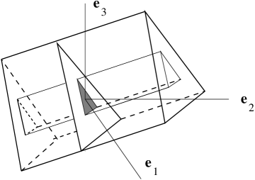
Figure 1: Example of a cylindrical $\Lambda$ embedded in $\mathbb{Z}^{3}$. A small cylindrical subvolume as used in the construction of the perturbed states is also shown.

We let $l(x)$ denote the signed distance from the origin: $l(x)=x^{1}+x^{2}+x^{3}$, where $x=(x^{1},x^{2},x^{3})\in\mathbb{Z}^{3}$. Then

$$B(\Lambda)=\{(x_{0},x_{1}):|x_{0}-x_{1}|=1,l(x_{1})=l(x_{0})+1\}$$ (2.1)

describes the set of oriented bonds in $\mathbb{Z}^{3}$. The infinite stick $\Sigma_{0}^{\infty}$ is, by definition, the set of vertices of the form

$$\ldots-e_{2}-e_{3},-e_{3},0,e_{1},e_{1}+e_{2},e_{1}+e_{2}+e_{3},e_{1}+e_{2}+e_{3}+e_{1},\ldots$$

For any even integer $L$, the finite stick $\Sigma_{0}$ of length $L+1$ is then given by

$$\Sigma_{0}=\{x\in\Sigma_{0}^{\infty}\mid-L/2\leq l(x)\leq L/2\}\quad.$$

We will take for $\Lambda$ is a cylindrical region whose axis points in the 111 direction, where by cylindrical we mean that $\Lambda$ can be obtained from a subset $\Gamma$ of the $l(x)=0$ plane, which we will call the base, by adding to all vertices $x\in\Gamma$ the finite stick $\Sigma_{0}$:

$$\Lambda=\{x+y\mid x\in\Gamma,y\in\Sigma_{0}\}$$

The equation $l(x)=c$, for any constant c, defines a cross-section of $\Lambda$, which contains exactly $A=|\Gamma|$ vertices. Hence, $|\Lambda|=(L+1)A$. We refer to these cross-sections as planes.

As an example, the projection onto the plane $l(x)=0$, of the vertices of $\Lambda$ with triangular base is shown in Figure 2, with different shades depending on the value of $l(x)$ modulo 3. The orientation of the bonds is indicated by arrows, and one may observe that each site on the interior of $\Lambda$ has an equal number of incoming and outgoing bonds.

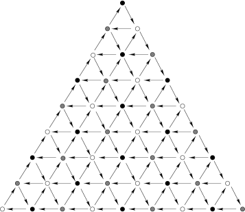
Figure 2: The projection onto the $111$ plane of a cylindrical volume $\Lambda$ with triangular base. The shading of the vertices depends on the value of $l(x)$ modulo 3. The orientation of the bonds is indicated by arrows. Observe that each site has an equal number of incoming and outgoing bonds.

By construction, $\Lambda$ can be decomposed into one-dimensional sticks running parallel to the cylindrical axis, which we will generically call $\Sigma$. (See Figure 3.) One should observe that $\Sigma$ is comprised entirely of nearest-neighbor pairs so that every site on $\Sigma$ is connected to every other site by a sequence of bonds. This will allows us to exploit the well-known properties of the one-dimensional Heisenberg XXZ model to describe $\Sigma$.

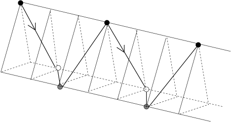
Figure 3: The bonds connecting the vertices of a stick $\Sigma$ form a one-dimensional subsystem.

The Hamiltonian for the spin-$\frac{1}{2}$ ferromagnetic $XXZ$ Heisenberg model is given by

$$H_{\Lambda}=\sum_{(x_{0},x_{1})\in B(\Lambda)}h^{q}_{x_{0},x_{1}},$$ (2.2)

where

$$h^{q}_{x_{0},x_{1}}=-\Delta^{-1}(S_{x_{0}}^{(1)}S_{x_{1}}^{(1)}+S_{x_{0}}^{(2)}S_{x_{1}}^{(2)})-S_{x_{0}}^{(3)}S_{x_{1}}^{(3)}+\frac{1}{4}+\frac{1}{4}A(\Delta)(S_{x_{1}}^{(3)}-S_{x_{0}}^{(3)}).$$ (2.3)

and $\Delta\geq 1$ is the “anisotropic coupling”, $A(\Delta)={1\over 2}\sqrt{1-1/\Delta^{2}}$, and $q$, $0<q<1$, is the solution of $\Delta={1\over 2}(q+q^{-1})$ The matrices $S_{x}^{(\alpha)}$ ($\alpha=1,2,3$) are the Pauli spin matrices acting on the site $x$,

$$S^{(1)}=\left[\begin{array}[]{cc}0&1/2\\ 1/2&0\end{array}\right],\quad S^{(2)}=\left[\begin{array}[]{cc}0&-i/2\\ i/2&0\end{array}\right],\quad S^{(3)}=\left[\begin{array}[]{cc}1/2&0\\ 0&-1/2\end{array}\right].$$ (2.4)

The terms containing $A(\Delta)$ cancel on all sites except at the top and bottom plane of the cylinder. The usefulness of the nearest-neighbor Hamiltonian stems from the fact that its action on any bond is given by

$$h^{q}\left|\downarrow\downarrow\right\rangle=0, \quad h^{q}\left|\downarrow\uparrow\right\rangle={1\over{q+q^{-1}}}\left(q\left|\downarrow\uparrow\right\rangle-\left|\uparrow\downarrow\right\rangle\right),$$

$$h^{q}\left|\uparrow\uparrow\right\rangle=0, \quad h^{q}\left|\uparrow\downarrow\right\rangle=-{1\over{q+q^{-1}}}\left(\left|\downarrow\uparrow\right\rangle-q^{-1}\left|\uparrow\downarrow\right\rangle\right).$$

In other words, $h^{q}$ is the orthogonal projection on the unit vector

$$\xi_{q}={1\over\sqrt{1+q^{2}}}(q\left|\downarrow\uparrow\right\rangle-\left|\uparrow\downarrow\right\rangle).$$ (2.5)

There is a $(|\Lambda|+1)$-fold degeneracy in the ground states with a unique ground state for each value of total third component of the spin $\sum_{x\in\Lambda}S^{(3)}_{x}$. The basis vectors of the Hilbert space $(\mathbb{C}^{2})^{\otimes|\Lambda|}$ can be labeled with particle configurations $\alpha=\{\alpha(x)\}_{x\in\Lambda}$, where $\alpha(x)$ is 0 or 1, corresponding to $\left|\uparrow\right\rangle$ and $\left|\downarrow\right\rangle$, respectively. We write $\mathsf{N}$ for the operator defined by

$$\mathsf{N}\left|\alpha\right\rangle=(\sum_{x\in\Lambda}\alpha(x))\left|\alpha\right\rangle,$$

and let $\mathcal{A}(\Lambda,n)$ denote the collection of all configurations with $\mathsf{N}(\alpha)=n$.

Following [1] the ground states are given by

$$\psi_{0}(\Lambda,n)=\sum_{\mathbf{\alpha}\in\mathcal{A}(\Lambda,n)}\bigotimes_{x\in\Lambda}q^{l(x)\alpha(x)}\left|\alpha(x)\right\rangle,$$ (2.6)

Note that the weights of $\alpha$ are invariant under any permutation of the sites for which planes are invariant. These states describe an interface located, on the average, in the plane determined by $(L/2+l_{x})A=n$ [8].

We denote $\|\psi_{0}(\Lambda,n)\|^{2}$ by $Z(\Lambda,n)$. This quantity is given by

$$Z(\Lambda,n)=\sum_{\mathbf{\alpha}\in\mathcal{A}(\Lambda,n)}\ \prod_{x\in\Lambda}q^{2l(x)\alpha(x)}$$ (2.7)

We will treat $Z(\Lambda,n)$ as a canonical partition function. It will be useful to consider, also, its grand canonical analogue:

$$Z^{GC}(\Lambda,\mu)=\sum_{n=0}^{L}Z(\Lambda,n)q^{-2\mu n}=\prod_{x\in\Lambda}(1+q^{2(l(x)-\mu)}).$$ (2.8)

Then it is easily seen that $Z^{GC}(\Lambda,\mu)$ is the squared-norm of the grand canonical vector defined by

$$\psi^{GC}(\Lambda,\mu)=\sum_{n=0}^{|\Lambda|}q^{-n\mu}\psi_{0}(\Lambda,n)=\bigotimes_{x\in\Lambda}(\left|\uparrow\right\rangle+q^{l(x)-\mu}\left|\downarrow\right\rangle).$$ (2.9)

Due to the product structure, the thermodynamic limit is simply given by

$$\langle{X}\rangle^{GC}_{\mathbb{Z}^{3},\mu}=\bigotimes_{x\in\mathbb{Z}^{3}}\frac{\left\langle\uparrow\right|+q^{l(x)-\mu}\left\langle\downarrow\right|}{\sqrt{1+q^{2(l(x)-\mu)}}}\;\;X\;\bigotimes_{x\in\mathbb{Z}^{3}}\frac{\left|\uparrow\right\rangle+q^{l(x)-\mu}\left|\downarrow\right\rangle}{\sqrt{1+q^{2(l(x)-\mu)}}}$$ (2.10)

for all local observables $X$.

3 Equivalence of Ensembles

A key step in our argument is the development of an equivalence of ensembles. Specifically, we will show that for a gauge-invariant local observable the canonical expectation is close to the grand canonical expectation for some suitably chosen chemical potential $\mu$. Here $\mu$ only depends on the total spin of the canonical ensemble, not on the form of the observable. From this, naturally follows a thermodynamic limit for gauge-invariant observables. We begin with activity bounds that show that the ratio of two canonical partition functions with different particle numbers is approximately exponential in the difference of the particle numbers, i.e.,

$$Z(\Lambda,n-k)\approx Z(\Lambda,n)q^{-2k\mu}$$

for $|k|\ll n$. More precisely, we have the following lemma.

Lemma 3.1 (Activity bounds)

For every volume ${\Lambda}$, $|{\Lambda}|=(L+1)A$, the ratio of canonical partition functions for different number of particles can be bounded from above and below by activity bounds as follows. Let $A_{0}$ be any constant. Suppose $n$, $0\leq n\leq A(L+1)$, and $\mu$ are such that

$$n-A\langle{\mathsf{N}}\rangle^{GC}_{\Sigma,\mu}\leq\frac{1}{2}A_{0}A^{1/2}.$$ (3.1)

Then, for every $k$ satisfying

$$|k|\leq\frac{1}{2}A_{0}A^{1/2},$$ (3.2)

one has the bounds

$$\frac{Z(\Lambda,n)}{Z(\Lambda,n-k)}\;\leq\;C(A_{0},A)q^{k[2\frac{n}{A}-2\langle{\mathsf{N}}\rangle^{GC}_{\Sigma,\mu}+2\mu a\sigma^{2}-\frac{k}{A}]/(a\sigma^{2})},$$ (3.3)

and

$$\frac{Z(\Lambda,n)}{Z(\Lambda,n-k)}\;\geq\;C(A_{0},A)^{-1}q^{k[2\frac{n}{A}-2\langle{\mathsf{N}}\rangle^{GC}_{\Sigma,\mu}+2\mu a\sigma^{2}-\frac{k}{A}]/(a\sigma^{2})},$$ (3.4)

where $a=2|\ln q|$,

$$\sigma^{2}:=\sigma^{2}(\mu,L)=\frac{1}{4}\sum_{l=-L/2}^{L/2}\frac{1}{\cosh^{2}(\frac{a}{2}(l-\mu))},$$

and

$$C(A_{0},A)=\frac{1+\frac{A_{0}}{\sigma^{2}A^{1/2}}}{1-\frac{A_{0}}{\sigma^{2}A^{1/2}}}.$$ (3.5)

Moreover, if $\mu$ is the solution of $\frac{n}{A}-\langle{\mathsf{N}}\rangle^{GC}_{\Sigma,\mu}=0$, then, also using the bounds for $\sigma^{2}$ given in (6.15), we obtain

$$C(A_{0}/2,A)^{-1}q^{-\frac{k^{2}(1-q^{2})}{2a(1+q^{2})A}}\leq q^{-2k\mu}\frac{Z(\Lambda,n)}{Z(\Lambda,n-k)}\leq C(A_{0}/2,A)q^{-\frac{2k^{2}(1-q^{2})}{aq^{2}A}}.$$ (3.6)

Alternatively, if $\mu$ solves $\frac{n-k}{A}-\langle{\mathsf{N}}\rangle^{GC}_{\Sigma,\mu}=0$, then we obtain

$$C(A_{0}/2,A)^{-1}q^{\frac{k^{2}(1-q^{2})}{2a(1+q^{2})A}}\leq q^{-2k\mu}\frac{Z(\Lambda,n)}{Z(\Lambda,n-k)}\leq C(A_{0}/2,A)q^{\frac{2k^{2}(1-q^{2})}{aq^{2}A}}.$$ (3.7)

Proof: This can be obtained as follows. Let consider the grand canonical probability

$$p(\mu,{\bf n})=q^{-2\mu|{\bf n}|}\frac{Z({\bf n})}{Z_{GC}(\mu)}\,;$$ (3.8)

with

$$Z({\bf n})=\sum_{\alpha:\mathcal{A}(\Sigma_{1},n_{1})\otimes\cdots\otimes\mathcal{A}(\Sigma_{A-A_{0}},n_{A-A_{0}})}q^{w(\alpha)}$$ (3.9)

where $\Sigma_{i}$ is the i-th one dimensional stick that we are decomposing our volume in, and where $Z_{GC}(\mu)$ is the grand-canonical partition function. Clearly, we have

$$Z(n)\,=\,\sum_{{\bf n}:|{\bf n}|=n}Z({\bf n})\;.$$ (3.10)

Define

$$p(\mu,n)\,=\,\sum_{{\bf n}:|{\bf n}|=n}p(\mu,{\bf n})\;,$$ (3.11)

and we have

$$\frac{Z(n)}{Z(n-k)}=\frac{p(\mu,n)}{p(\mu,n-k)}q^{2k\mu}$$ (3.12)

The idea now is to make use of the local central limit theorem for the probability distribution of the occupation number in the i-th stick (see [4] Theorem XVI.4.3.). Let $\xi_{i}=\sum_{x\in\Sigma_{i}}\alpha_{x}$. For any integer $N$, consider, the probability

$$P_{\mu}(\xi_{1}=n_{1},...,\xi_{N}=n_{N})\,=\,p(\mu,{\bf n})\,.$$ (3.13)

Due to the factorization property of $p(\mu,{\bf n})$, the $\xi$’s are independent identically distributed random variables. For centered i.i.d. random variables $X_{i}$ with variance $\sigma^{2}$, the local central limit theorem guarantees that the random variable

$$S_{N}=\frac{1}{\sigma\sqrt{N}}\sum_{n=1}^{N}X_{n}\quad.$$ (3.14)

is close to a Gaussian in the sense that the quantity

$$P_{N}(x):={\rm Prob}(\sum_{n=1}^{N}X_{n}=x)$$ (3.15)

fulfills the bounds

$$\frac{1}{\sigma\sqrt{2\pi N}}e^{-\frac{x^{2}}{2\sigma^{2}N}}\left(1-\frac{c}{\sqrt{N}}\right)\leq P_{N}(x)\leq\frac{1}{\sigma\sqrt{2\pi N}}e^{-\frac{x^{2}}{2\sigma^{2}N}}\left(1+\frac{c}{\sqrt{N}}\right)$$ (3.16)

where $c$ is the constant

$$c=\frac{\max(|x|,|x-k|)}{\sigma^{2}\sqrt{N}}.$$ (3.17)

By applying (3.16) to the centered quantity $X_{n}=\xi_{n}-\langle{\xi_{n}}\rangle$, we obtain the following bounds on the ratio of probabilities:

$$C(N)^{-1}e^{-k(2x-k)/2\sigma^{2}N}\leq\frac{P_{N}(x)}{P_{N}(x-k)}\leq C(N)e^{-k(2x-k)/2\sigma^{2}N}$$ (3.18)

where

$$C(N)=\frac{1+cN^{-1/2}}{1-cN^{-1/2}}\quad.$$ (3.19)

In terms of the non-centered variables $\xi_{i}$ we have

$$p(\mu,n)\;=\;P_{A}\left(n-A\langle{\mathsf{N}}\rangle^{GC}_{\Sigma,\mu}\right)$$ (3.20)

where $\langle{\mathsf{N}}\rangle^{GC}_{\Sigma,\mu}$ is the average number of particles of a 1D stick $\Sigma$, in the grand canonical ensemble with chemical potential $\mu$. From this and the hypotheses (3.1), (3.2), we obtain

$$c=\frac{A_{0}}{\sigma^{2}}\quad\textrm{ and }\quad C(A_{0},A)=\frac{1+\frac{A_{0}}{\sigma^{2}A^{1/2}}}{1-\frac{A_{0}}{\sigma^{2}A^{1/2}}}.$$ (3.21)

Note that in case $\mu$ is chosen so that $\langle{\mathsf{N}}\rangle^{GC}_{\Sigma,\mu}=n/A$ or $\langle{\mathsf{N}}\rangle^{GC}_{\Sigma,\mu}=(n-k)/A$ then we can replace $c$ by $c/2$, with the result that $C(A_{0},A)$ may be replaced by

$$C(A_{0}/2,A)=\frac{1+\frac{A_{0}}{2\sigma^{2}A^{1/2}}}{1-\frac{A_{0}}{2\sigma^{2}A^{1/2}}},$$

as well.
Also, from (3.20) and (3.18), we have

$$C(A_{0},A)^{-1}e^{-\frac{k(2n-2A\langle{\mathsf{N}}\rangle^{GC}_{\Sigma,\mu}-k)}{2\sigma^{2}A}}\leq\frac{p(\mu,n)}{p(\mu,n-k)}\leq C(A_{0},A)e^{-\frac{k(2n-2A\langle{\mathsf{N}}\rangle^{GC}_{\Sigma,\mu}-k)}{2\sigma^{2}A}}.$$ (3.22)

Using (3.12) (and observing that $q^{2\mu k}=e^{-a\mu}$), we have

$$\frac{Z(n)}{Z(n-k)}\;\leq\;C(A_{0},A)e^{-k[2\frac{n}{A}-2\langle{\mathsf{N}}\rangle^{GC}_{\Sigma,\mu}+2a\sigma^{2}\mu-\frac{k}{A}]/2\sigma^{2}}\;,$$ (3.23)

and

$$\frac{Z(n)}{Z(n-k)}\;\geq\;C(A_{0},A)e^{-k[2\frac{n}{A}-2\langle{\mathsf{N}}\rangle^{GC}_{\Sigma,\mu}+2a\sigma^{2}\mu-\frac{k}{A}]/2\sigma^{2}}\;.$$ (3.24)

Changing to base $q$ then leads to equations (3.3) and (3.4) of the theorem. By the derivation of Section 6.2, we have the bounds on the variance for the number of particles in a 1D stick:

$$\frac{1}{4}\frac{q^{2}}{1-q^{2}}\leq\sigma^{2}(\mu)\leq\frac{1+q^{2}}{1-q^{2}}.$$ (3.25)

In conjunction with the remark about replacing $C(A_{0},A)$ by $C(A_{0}/2,A)$, this gives equations (3.6) and (3.7).  

As an application of this lemma, let us consider the case where $n$ is replaced by $\rho|\Lambda|-n_{0}$, $k$ is replaced by $\rho|\Lambda_{0}|-n_{0}$ and $\Lambda$ is replaced by $\Lambda_{0}^{c}:=\Lambda\setminus\Lambda_{0}$. This means that in the lemma $A$ is replaced by $A-A_{0}$, and $(n-k)/A$ is replaced by $\rho(|\Lambda|-|\Lambda_{0}|)/(A-A_{0})=\rho(L+1)$. Then, direct substitution shows

$$\frac{Z(\Lambda_{0}^{c},\rho|\Lambda|-n_{0})}{Z(\Lambda_{0}^{c},\rho|\Lambda_{0}^{c}|)}$$

$$\qquad\leq C(A_{0}/2,A-A_{0})\,q^{-2k\mu}e^{-k[2\rho(L+1)-2\langle{\mathsf{N}}\rangle^{GC}_{\Sigma,\mu}+\frac{k}{A-A_{0}}]/2\sigma^{2}},$$ (3.26)

$$\frac{Z(\Lambda_{0}^{c},\rho|\Lambda|-n_{0})}{Z(\Lambda_{0}^{c},\rho|\Lambda_{0}^{c}|)}\;$$

$$\qquad\geq C(A_{0}/2,A-A_{0})^{-1}\,q^{-2k\mu}e^{-k[2\rho(L+1)-2\langle{\mathsf{N}}\rangle^{GC}_{\Sigma,\mu}+\frac{k}{A-A_{0}}]/2\sigma^{2}},$$ (3.27)

where we have retained $k$, for the moment. If, further, we choose $\mu$ so that $\langle{\mathsf{N}}\rangle^{GC}_{\Sigma,\mu}=\rho(L+1)$, which is always possible (see Section 6.3), then, by equation (3.7), we have

$$q^{2\mu k}\frac{Z(\Lambda_{0}^{c},\rho|\Lambda|-n_{0})}{Z(\Lambda_{0}^{c},\rho|\Lambda_{0}^{c}|)}\;\leq\;C(A_{0}/2,A-A_{0})\,e^{-\frac{k^{2}}{2(A-A_{0})\sigma^{2}}},$$ (3.28)

$$q^{2\mu k}\frac{Z(\Lambda_{0}^{c},\rho|\Lambda|-n_{0})}{Z(\Lambda_{0}^{c},\rho|\Lambda_{0}^{c}|)}\;\geq\;C(A_{0}/2,A-A_{0})^{-1}\,e^{-\frac{k^{2}}{2(A-A_{0})\sigma^{2}}}.$$ (3.29)

Using our bounds for $\sigma^{2}$, we have

$$q^{2\mu k}\frac{Z(\Lambda_{0}^{c},\rho|\Lambda|-n_{0})}{Z(\Lambda_{0}^{c},\rho|\Lambda_{0}^{c}|)}\;\leq\;C(A_{0}/2,A-A_{0})\,e^{-\frac{(1-q^{2})k^{2}}{2(1+q^{2})(A-A_{0})}},$$ (3.30)

$$q^{2\mu k}\frac{Z(\Lambda_{0}^{c},\rho|\Lambda|-n_{0})}{Z(\Lambda_{0}^{c},\rho|\Lambda_{0}^{c}|)}\;\geq\;C(A_{0}/2,A-A_{0})^{-1}\,e^{-\frac{2(1-q^{2})k^{2}}{2q^{2}(A-A_{0})}}.$$ (3.31)

By our choice of $\mu$, conditions (3.1) and (3.2) are satisfied as long as the order of $L$ does not exceed the order of $(A-A_{0})^{1/2}$. This estimate will be of use in the next theorem.

Let $\|X\|_{gs}$ denote the operator-norm of $X$ restricted to the subspace of ground states. For observables $X$, localized in $\Lambda$ and commuting with $J^{(3)}$, $\|X\|_{gs}$ is also given by

$$\|X\|_{gs}=\sup_{0\leq n\leq|\Lambda|}|\langle{X}\rangle_{\Lambda,n}|.$$

Theorem 3.2 (Equivalence of Ensembles)

Consider two cylindrical volumes $\Lambda$ and $\Lambda_{0}$, $\Lambda_{0}\subset\Lambda$, of the type defined in Section 2 (in particular $|\Lambda|=A(L+1)$, $|\Lambda_{0}|=A_{0}(L+1)$), and fix a total number of particles $n_{\Lambda}$. Define $\rho=n_{\Lambda}/|\Lambda|$. Suppose $X$ is a local observable in the volume $\Lambda_{0}$, which commutes with $J^{(3)}:=\sum_{x}S^{(3)}_{x}$. Then we have

$$|\langle{X}\rangle_{\Lambda,n}-\langle{X}\rangle^{GC}_{\Lambda_{0},\mu}|\;\leq\;\varepsilon\|X\|_{gs}\;,$$ (3.32)

where

$$\varepsilon=\frac{\ln^{2}(A-A_{0})+2(1+a^{2})A_{0}^{2}+4}{2(A-A_{0})}+\frac{4A_{0}}{q^{2}(A-A_{0})^{1/2}-2A_{0}},$$ (3.33)

$a=2|\ln q|$, and the chemical potential $\mu$ is determined by the equation

$$\langle{\mathsf{N}}\rangle^{GC}_{\Sigma,\mu}=\rho(L+1).$$ (3.34)

In particular, for $\rho=1/2$ the calculations of Section 6.1 will show that $\mu=0$.

Corollary 3.3 (Existence of the Thermodynamic limit)

(i) Suppose we have a sequence of pairs $(\Lambda_{k},n_{k})$ with $\Lambda_{k}$ cylindrical volumes and $\Lambda_{k}\nearrow\mathbb{Z}^{3}$ in such a way that the length does not grow faster than the linear size of the base. Let $\mu_{k}$ solve $\langle{\mathsf{N}}\rangle^{GC}_{\Lambda_{k},\mu_{k}}=n_{k}$. Then the convergence $\mu_{k}\to\mu$ guarantees the convergence, of $\langle{.}\rangle_{\Lambda_{k},n_{k}}$ to $\langle{.}\rangle^{GC}_{\mathbb{Z}^{3},\mu}$, for all local observables $X$ commuting with $J^{(3)}$ :

$$\langle{X}\rangle_{\Lambda_{k},n_{k}}\to\langle{X}\rangle^{GC}_{\mathbb{Z}^{3},\mu}$$ (3.35)

(ii) Moreover, for any choice of $\mu$, we may find a sequence of pairs $(\Lambda_{k},n_{k})$ such that

$$\langle{X}\rangle_{\Lambda_{k},n_{k}}\to\langle{X}\rangle^{GC}_{\mathbb{Z}^{3},\mu}.$$ (3.36)

Proof: (Proof of Corollary) It follows from the monotonicity of $\langle{\mathsf{N}}\rangle^{GC}_{\Sigma,\mu}$ proved in Section 6.1, that the equation

$$\langle{\mathsf{N}}\rangle^{GC}_{\Lambda_{k},\mu_{k}}=n_{k}$$ (3.37)

always has a unique solution for $\mu_{k}$. Then, (i) follows immediately from the inequality (3.32), once we observe that $\epsilon\searrow 0$ as $\Lambda\nearrow\mathbb{Z}^{3}$ in the sense prescribed in the corollary.
For (ii), take $\Lambda_{k}$, with base $A_{k}$, and $n_{k}$ such that

$$n_{k}=\lfloor{A_{k}\langle{\mathsf{N}}\rangle^{GC}_{\Sigma,\mu}}\rfloor\quad.$$

where $\lfloor{x}\rfloor$ denotes the largest integer $\leq x$. Then, $\mu_{k}$ solving (3.37), is easily seen to converge to $\mu$, and (3.36) follows from (i).  

The interpretation of the condition $\mu_{k}\to\mu$ in (i) of the Corollary is that, not only does $n_{k}/|\Lambda_{k}|$ converge to $\rho=1/2$, but, more precisely

$$n_{k}=\rho|\Lambda_{k}|+\nu A_{k}+o(A_{k})\quad.$$

The term proportional to $|\Lambda_{k}|$ guarantees that the interface is in the center of the volume, the second term fixes its filling factor.

Proof: (Proof of Theorem 3.2) Let $\mu$ be determined by (3.34), and define $\Xi$ as follows:

$$\Xi=\frac{Z(\Lambda,n_{\Lambda})q^{-2\mu\rho|\Lambda_{0}|}}{Z(\Lambda_{0}^{c},\rho|\Lambda_{0}^{c}|)Z^{GC}(\Lambda_{0},\mu)}$$ (3.38)

where $\Lambda_{0}^{c}:=\Lambda\setminus\Lambda_{0}$. We will obtain the equivalence of ensembles by combining two facts. The first is that $\Xi$ is approximately equal to $1$, and the second is an estimate showing that

$$|\langle{X}\rangle_{\Lambda,n_{\Lambda}}\Xi-\langle{X}\rangle^{GC}_{\Lambda_{0},\mu}|\leq\varepsilon\|X\|_{gs}$$

But first, let us recall the definitions of the expectation of an observable $X$:

$$\langle{X}\rangle_{\Lambda,n} = \frac{\left\langle\psi(\Lambda,n)\right|X\left|\psi(\Lambda,n)\right\rangle}{\langle{\psi(\Lambda,n)|\psi(\Lambda,n)}\rangle},$$ (3.39)

$$\langle{X}\rangle^{GC}_{\Lambda,\mu} = \frac{\left\langle\psi^{GC}(\Lambda,\mu)\right|X\left|\psi^{GC}(\Lambda,\mu)\right\rangle}{\langle{\psi^{GC}(\Lambda,\mu)|\psi^{GC}(\Lambda,\mu)}\rangle}.$$ (3.40)

Since $X$ is an observable localized in $\Lambda_{0}$, we note that $\langle{X}\rangle^{GC}_{\Lambda,\mu}=\langle{X}\rangle^{GC}_{\Lambda_{0},\mu}$. Moreover, we may decompose the grand canonical state into a superposition of canonical states:

$$\psi^{GC}(\Lambda_{0},\mu)=\sum_{n_{0}=0}^{|\Lambda_{0}|}q^{-\mu n_{0}}\psi(\Lambda_{0},n_{0}).$$ (3.41)

Since $X$ commutes with $J^{(3)}$, it does not have off-diagonal matrix elements between these canonical states with all different values of the total spin. Therefore,

$$\langle{X}\rangle^{GC}_{\Lambda,\mu}=Z^{GC}(\Lambda,\mu)^{-1}\sum_{n_{0}=0}^{|\Lambda_{0}|}q^{-2\mu n_{0}}Z(\Lambda_{0},n_{0})\langle{X}\rangle_{\Lambda_{0},n_{0}}.$$ (3.42)

Note also, that since we have a decomposition

$$\psi(\Lambda,n)=\sum_{n_{0}=0}^{|\Lambda_{0}|}\psi(\Lambda\setminus\Lambda_{0},n-n_{0})\otimes\psi(\Lambda_{0},n_{0}),$$ (3.43)

and using the previously described properties, we have

$$\langle{X}\rangle_{\Lambda,n} = \sum_{n_{0}=0}^{|\Lambda_{0}|}\frac{Z(\Lambda\setminus\Lambda_{0},n-n_{0})Z(\Lambda_{0},n_{0})}{Z(\Lambda,n)}\langle{X}\rangle_{\Lambda_{0},n_{0}}$$ (3.45)

$$= Z^{GC}(\Lambda_{0},\mu)^{-1}\sum_{n_{0}=0}^{|\Lambda_{0}|}q^{-2\mu n_{0}}Z(\Lambda_{0},n_{0})\langle{X}\rangle_{\Lambda_{0},n_{0}}\times$$

$$\quad\times\frac{Z(\Lambda_{0}^{c},n-n_{0})Z^{GC}(\Lambda_{0},\mu)}{q^{-2\mu n_{0}}Z(\Lambda,n)}.$$

This differs from the definition of $\langle{X}\rangle^{GC}_{\Lambda_{0},\mu}$ only by the final factor, which is a ratio of partition functions hence amenable to our activity bounds.
In fact, we have

$$\langle{X}\rangle_{\Lambda,n}\Xi-\langle{X}\rangle^{GC}_{\Lambda,\mu} = Z^{GC}(\Lambda_{0},\mu)^{-1}\sum_{n_{0}=0}^{|\Lambda_{0}|}q^{-2\mu n_{0}}\langle{X}\rangle_{\Lambda_{0},n_{0}}Z(\Lambda_{0},n_{0})\times$$ (3.46)

$$\quad\times\left[q^{2\mu(n_{0}-\langle{n_{0}}\rangle)}\ \frac{Z(\Lambda_{0}^{c},n-n_{0})}{Z(\Lambda_{0}^{c},\lfloor{\rho|\Lambda_{0}|}\rfloor)}-1\right]$$

where $\langle{n_{0}}\rangle=\langle{\mathsf{N}}\rangle^{GC}_{\Lambda_{0},\mu}$, which equals $\rho|\Lambda_{0}|$ for our choice of $\mu$. Thus we obtain $|\langle{X}\rangle_{\Lambda,n}\Xi-\langle{X}\rangle^{GC}_{\Lambda,\mu}|\leq\|X\|_{gs}\langle{|g|}\rangle^{GC}_{\Lambda_{0},\mu},$ where

$$g=q^{2\mu(n_{0}-\langle{n_{0}}\rangle)}\ \frac{Z(\Lambda_{0}^{c},n-n_{0})}{Z(\Lambda_{0}^{c},\lfloor{\rho|\Lambda_{0}|}\rfloor)}-1.$$ (3.47)

Now we use the activity bounds (3.30) and (3.31), but replacing $k$ by its actual value, $\langle{n_{0}}\rangle-n_{0}$. We arrive at the bounds

$$g \leq g_{1}:=C(A_{0}/2,A-A_{0})e^{-\frac{(1-q^{2})(\langle{n_{0}}\rangle-n_{0})^{2}}{2(1+q^{2})(A-A_{0})}}-1,$$ (3.48)

$$g \geq g_{2}:=C(A_{0}/2,A-A_{0})^{-1}e^{-\frac{2(1-q^{2})(\langle{n_{0}}\rangle-n_{0})^{2}}{2q^{2}(A-A_{0})}}-1,$$ (3.49)

where

$$C(A_{0}/2,A-A_{0})=\frac{1+\frac{A_{0}}{2\sigma^{2}(A-A_{0})^{1/2}}}{1-\frac{A_{0}}{2\sigma^{2}(A-A_{0})^{1/2}}}.$$ (3.50)

Therefore, $|g|\leq\max(|g_{1}|,|g_{2}|)\leq|g_{1}|+|g_{2}|$.
We now use the triangle inequality and the fact that the exponent is negative to obtain:

$$|g_{1}|\leq\left|1-e^{-\frac{(1-q^{2})(\langle{n_{0}}\rangle-n_{0})^{2}}{2(1+q^{2})(A-A_{0})}}\right|+|1-C(A_{0}/2,A-A_{0})|,$$ (3.51)

so that

$$\langle{|g_{1}|}\rangle_{\Lambda_{0},\mu}\leq\langle{1-e^{-\frac{(1-q^{2})(\langle{n_{0}}\rangle-n_{0})^{2}}{2(1+q^{2})(A-A_{0})}}}\rangle^{GC}_{\Lambda_{0},\mu}+C(A_{0}/2,A-A_{0})-1.$$ (3.52)

Similarly,

$$\langle{|g_{2}|}\rangle_{\Lambda_{0},\mu}\leq\langle{1-e^{-\frac{2(1-q^{2})(\langle{n_{0}}\rangle-n_{0})^{2}}{2q^{2}(A-A_{0})}}}\rangle^{GC}_{\Lambda_{0},\mu}+1-C(A_{0}/2,A-A_{0})^{-1}.$$ (3.53)

We will use the Chebyshev inequality to control the expectation term in (3.52). Specifically, for any $B>0$,

$$\langle{1-e^{-\frac{(1-q^{2})(\langle{n_{0}}\rangle-n_{0})^{2}}{2(1+q^{2})(A-A_{0})}}}\rangle^{GC}_{\Lambda_{0},\mu} \leq {\rm Prob}(2|n_{0}-\langle{n_{0}}\rangle|\geq 2B)+1-e^{-\frac{(1-q^{2})B^{2}}{2(1+q^{2})(A-A_{0})}}$$

$$\leq q^{2B}\langle{q^{-2|n_{0}-\langle{n_{0}}\rangle|}}\rangle^{GC}_{\Lambda_{0},\mu}+1-e^{-\frac{(1-q^{2})B^{2}}{2(1+q^{2})(A-A_{0})}}.$$

In Section 6.3 we show that $\langle{q^{-2|n_{0}-\langle{n_{0}}\rangle|}}\rangle^{GC}_{\Lambda_{0},\mu}\leq 2(2q^{-2})^{A_{0}}$. One choice for $B$ is $a^{-1}[\ln(A-A_{0})+A_{0}\ln(2q^{-2})]$. This gives the bound

$$\langle{1-q^{\frac{(n_{0}-\langle{n_{0}}\rangle)^{2}}{A-A_{0}}}}\rangle^{GC}_{\Lambda_{0},\mu} \leq \frac{2+\frac{1-q^{2}}{a^{2}(1+q^{2})}\left[2(1+a^{2})A_{0}^{2}+\ln^{2}(A-A_{0})\right]}{A-A_{0}}$$

$$\leq \frac{2+(1+a^{2})A_{0}^{2}+\frac{1}{2}\ln^{2}(A-A_{0})}{A-A_{0}}$$

$$=: C_{1}(A,A_{0},q)$$

The leading order term in the bound is $\frac{\ln^{2}(A-A_{0})}{2(A-A_{0})}$ for fixed $q$, strictly between 0 and 1. Also, let

$$C_{2}(q,A,A_{0})=\frac{4A_{0}}{q^{2}(A-A_{0})^{1/2}-2A_{0}},$$ (3.55)

which is greater than both $C(A_{0}/2,A-A_{0})-1$ and $1-C(A_{0}/2,A-A_{0})^{-1}$. Then $|\langle{f}\rangle_{\Lambda,n}\Xi-\langle{f}\rangle^{GC}_{\Lambda,\mu}|\leq(C_{1}+C_{2})\|X\|_{gs}$. In particular, $|\langle{1\hskip-3.0pt\rm{I}}\rangle_{\Lambda,n}\Xi-\langle{1\hskip-3.0pt\rm{I}}\rangle^{GC}_{\Lambda,\mu}|\leq(C_{1}+C_{2})\|1\hskip-3.0pt\rm{I}\|_{gs}$, which is to say that $|\Xi-1|\leq C_{1}+C_{2}$. Then, using the triangle inequality, we have

$$|\langle{X}\rangle_{\Lambda,n}-\langle{X}\rangle^{GC}_{\Lambda,\mu}| \leq |1-\Xi|\cdot|\langle{X}\rangle_{\Lambda,n}|+|\langle{X}\rangle_{\Lambda,n}\Xi-\langle{X}\rangle^{GC}_{\Lambda,\mu}|$$

$$\leq 2(C_{1}+C_{2})\|X\|_{gs}.$$

So, defining $\varepsilon=2C_{1}(q,\Lambda,\Lambda_{0},n)+2C_{2}(q,\Lambda,\Lambda_{0})$, the theorem is proved.  

Note that the restriction to observables $X$ that commute with the third component of the total spin $J^{(3)}$ is necessary. E.g., the expectation of $S^{+}_{x}$ obviously vanishes in any canonical state, while it is easy to see, by direct computation, that it does not vanish in the grand canonical states. This is entirely analogous to the restriction to gauge invariant observables in particle systems.

4 Bound on the energy

In this section we will estimate the energy of a class of perturbations of the ground state $\psi_{0}$ given in (2.6). Let $\Lambda$ and $\Lambda_{R}$ be two cylindrical volumes as described in Section 2, $\Lambda_{R}\subset\Lambda$. E.g., $\Lambda_{R}$ and $\Lambda$, may have triangular cross-sections (see Figure 1). We will generally assume that the radius $R$ of $\Lambda_{R}$ is much less than that of $\Lambda$. We consider $\psi$ of the form

$$\psi(\Lambda,n,\phi)=\sum_{\mathbf{\alpha}\in\mathcal{A}(\Lambda,n)}\bigotimes_{x\in\Lambda}e^{i\phi(x)\alpha(x)}q^{l(x)\alpha(x)}\left|\alpha(x)\right\rangle,$$ (4.1)

where ${\rm supp}(\phi)\subset\Lambda_{R}$.

We will also suppose that

$$\phi=\frac{\mathcal{S}}{R}\tilde{\phi}(\tilde{y}_{1},\tilde{y}_{2})$$ (4.2)

where $\tilde{\phi}$ is a smooth functions of its variables and $\mathcal{S}$ is a parameter, which we will eventually take to zero independent of $R$. The coordinates $\tilde{y}^{1},tilde{y}^{2}$, are defined by

$$\tilde{y}^{1}=\frac{2x^{1}-x^{2}-x^{3}}{\sqrt{6}R}\quad{\rm and}\quad\tilde{y}^{2}=\frac{x^{2}-x^{3}}{\sqrt{2}R},$$ (4.3)

and are to be viewed as rescaled coordinates for $x$ along the plane perpendicular to the 111 axis.

There are two points to our assumptions on $\phi$: First, that $\phi$ is independent of the 111 component of $x$. Second, that $\phi$ is associated to a scale-invariant phase $\tilde{\phi}$ by $\phi(x)=R^{-1}\tilde{\phi}(x/R)$. Ultimately, the constant $\mathcal{S}$ will vanish. The leading term in our estimate of the gap is independent of $\mathcal{S}$ as long as $\mathcal{S}\ll 1$.

Let $\Gamma_{R}$ be the projection of $\Lambda_{R}$ onto the plane $l(x)=0$, $A_{R}=|\Gamma_{R}|$, $\Omega_{R}$ be the convex hull of $\Gamma_{R}$, and $\tilde{\Omega}=\{x\in\mathbb{R}^{2}:Rx\in\Omega_{R}\}$, the rescaled region, and let $m(\tilde{\Omega})$ be the area of $\tilde{\Omega}$ (for the standard Lebesgue measure on $\mathbb{R}^{2}$).

We will also use the following notation: $\partial_{\tilde{y}}\tilde{\phi}$ and $\partial^{2}_{\tilde{y}}\tilde{\phi}$ are the first- and second-derivative tensors of $\tilde{\phi}$, and by the $L^{\infty}$ norm of a tensor we mean the maximum of the $L^{\infty}$ norms of the components.

Then we have the following theorem.

Theorem 4.1 (Bound on $\frac{\left\langle\psi\right|H^{(q)}_{\Lambda}\left|\psi\right\rangle}{\|\psi\|^{2}}$)

Considering a perturbed state as in (4.1), the energy is bounded by

$$\frac{\langle\psi\mid H^{(q)}_{\Lambda}\mid\psi\rangle}{\|\psi\|^{2}}\leq 2\frac{1+q^{2}}{1-q^{2}}\left(\frac{A_{R}\mathcal{S}^{2}}{R^{4}}\frac{\|\nabla_{\tilde{y}}\tilde{\phi}\|_{L^{2}(\tilde{\Omega})}^{2}}{m(\tilde{\Omega})}+\mathcal{E}_{\textrm{num}}\right)$$ (4.4)

where

$$\mathcal{E}_{\textrm{num}}=\frac{6A_{R}\mathcal{S}^{2}}{R^{5}}\|\partial_{\tilde{y}}^{2}\tilde{\phi}\|_{L^{\infty}}\|\partial_{\tilde{y}}\tilde{\phi}\|_{L^{\infty}}$$ (4.5)

is a correction to the main term which becomes negligible as $R\to\infty$.

Proof: We begin by calculating how a two-site hamiltonian $h_{b}^{q}$ acts on the perturbed state.

We consider the decomposition of our lattice into the relevant bond $b=(x_{0},x_{1})$ and everything else $\Lambda\setminus b$. Thus

$$h_{b}^{q}=1\hskip-3.0pt\rm{I}_{\Lambda\setminus b}\otimes\left|\xi_{b}\right\rangle\left\langle\xi_{b}\right|,$$ (4.6)

where $\xi_{b}$ is the unit vector from (2.5) on the pair $b$, and

$$\psi(\Lambda,n)=\sum_{n_{b}=0}^{2}\psi(\Lambda\setminus b,n-n_{b})\otimes\psi(b,n_{b}).$$ (4.7)

Here $\psi(b,n_{b})$ is as would be defined by (4.1), but with $\Lambda$ replaced by $b$ and $n$ replaced by $n_{b}$. For example $\psi(b,1)=q^{l(x_{0})}e^{i\phi(x_{0})}\left|\downarrow\uparrow\right\rangle+q^{l(x_{1})}e^{i\phi(x_{1})}\left|\uparrow\downarrow\right\rangle$. But $\xi_{b}$ is orthogonal to $\psi(b,0)$ and $\psi(b,1)$, since $\xi_{b}$ lies in the sector of total spin 1. And

$$\langle{\xi_{b}|\psi(b,1)}\rangle=\frac{1}{\sqrt{1+q^{2}}}q^{l(x_{0})+1}e^{i\phi(x_{0})}(1-e^{i[\phi(x_{1})-\phi(x_{0})]}).$$ (4.8)

Now it is straightforward to see

$$\left\langle\psi(\Lambda,n)\right|h_{b}^{q}\left|\psi(\Lambda,n)\right\rangle$$ (4.9)

$$\quad=\|\psi(\Lambda\setminus b,n-1)\|^{2}\,|\langle{\xi_{b}|\psi(b,1)}\rangle|^{2}$$

$$\quad=\frac{2}{(q+q^{-1})^{2}}Z(\Lambda,n)P^{q}(b)(1-\cos[\phi(x_{1})-\phi(x_{0})]),$$ (4.10)

where we have defined

$$P^{q}(b)=\frac{Z(\Lambda\setminus b,n-1)Z(b,1)}{Z(\Lambda,n)}.$$ (4.11)

Then we may write

$$\frac{\langle\psi\mid H^{(q)}_{\Lambda}\mid\psi\rangle}{Z(\Lambda,n)}=\frac{2}{(q+q^{-1})^{2}}~{}\sum_{b\in B(\Lambda)}\ P^{q}(b)(1-\cos[\phi(x_{1})-\phi(x_{0})]).$$ (4.12)

Actually, $P^{q}(b)$ depends on $b$ only through $l(x_{0})$. So from here on, we’ll write it as $P^{q}(l(x_{0}))$, and observe the following:

$$\frac{\langle\psi\mid H^{(q)}_{\Lambda}\mid\psi\rangle}{Z(\Lambda,n)}=\frac{2}{(q+q^{-1})^{2}}\sum_{l=-L/2}^{L/2-1}P^{q}(l)\sum_{x\in\Gamma^{l}_{R}}\sum_{j=1}^{3}(1-\cos[\phi(x+e_{j})-\phi(x)]),$$ (4.13)

where $\Gamma^{l}_{R}=\{x\in\Lambda_{R}:l(x)=l\}$.

Let us estimate the term $\sum_{x\in\Gamma^{l}_{R}}\sum_{j=1}^{3}(1-\cos[\phi(x+e_{j})-\phi(x)])$. We have an inequality

$$1-\cos[\phi(x+e_{j})-\phi(x)]\leq\frac{1}{2}[\phi(x+e_{j})-\phi(x)]^{2}$$ (4.14)

(which is actually an equality in the limit $R\to\infty$ for our ansatz). Also,

$$\sum_{i=1}^{3}[\phi(x+e_{j})-\phi(x)]^{2}\approx|\nabla_{x}\phi(x)|^{2}=\frac{\mathcal{S}^{2}}{R^{4}}|\nabla_{\tilde{y}}\tilde{\phi}|^{2}$$ (4.15)

In fact, using the inequality

$$|[\tilde{\phi}(\tilde{y}+v)-\tilde{\phi}(\tilde{y})]^{2}-[c\cdot\nabla_{\tilde{y}}\tilde{\phi}(\tilde{y})]^{2}|\leq\|\partial_{\tilde{y}}^{2}\tilde{\phi}\|_{L^{\infty}}\|\partial_{\tilde{y}}\tilde{\phi}\|_{L^{\infty}}\|v\|_{l^{1}}^{3}$$ (4.16)

one may conclude that the error in (4.15) is bounded by $\frac{3\mathcal{S}^{2}}{R^{5}}\|\partial_{\tilde{y}}^{2}\tilde{\phi}\|_{L^{\infty}}\|\partial_{\tilde{y}}\tilde{\phi}\|_{L^{\infty}}$.

Incorporating this estimate into the inequality of (4.14), we have

$$\sum_{x\in\Gamma^{l}_{R}}\sum_{j=1}^{3}(1-\cos[\phi(x+e_{j})-\phi(x)])\leq\qquad\qquad$$

$$\qquad\qquad\frac{1}{2R^{2}}\sum_{x\in\Gamma^{l}_{R}}|\nabla_{\tilde{y}}\phi(x)|^{2}+\frac{3\mathcal{S}^{2}|\Gamma^{l}_{R}|}{2R^{5}}\|\partial_{\tilde{y}}^{2}\tilde{\phi}\|_{L^{\infty}}\|\partial_{\tilde{y}}\tilde{\phi}\|_{L^{\infty}}$$ (4.17)

Finally, as $R\to\infty$, the sum over each $\Gamma^{l}_{R}$ becomes increasingly well-approximated by the integral over $\Omega_{R}$, we is proved in Lemma 4.2 immediately following this proof. The lemma gives us a bound

$$\sum_{x\in\Gamma^{l}_{R}}|\nabla_{\tilde{y}}\phi(x)|^{2}\leq\frac{\mathcal{S}^{2}|\Gamma^{l}_{R}|}{R^{2}}\left[\frac{1}{m(\tilde{\Omega})}\int_{\tilde{\Omega}}|\nabla_{\tilde{y}}\tilde{\phi}|^{2}\,d^{2}y+\frac{\rho}{R}\|\nabla^{2}_{\tilde{y}}\tilde{\phi}\nabla_{\tilde{y}}\tilde{\phi}\|_{L^{\infty}(\tilde{\Omega})}\right],$$ (4.18)

where $\nabla^{2}$ is the Laplacian and $\rho=\sqrt{2/3}$ is the maximum radius for the Voronoi domain. (Note that by its definition, as the trace of the second-derivative tensor, the Laplacian enjoys the bounds

$$\|\nabla^{2}_{\tilde{y}}\tilde{\phi}\nabla_{\tilde{y}}\tilde{\phi}\|_{L^{\infty}(\tilde{\Omega})}\leq 2\|\partial_{\tilde{y}}^{2}\tilde{\phi}\|_{L^{\infty}}\|\partial_{\tilde{y}}\tilde{\phi}\|_{L^{\infty}},$$ (4.19)

which may be combined with error term in (4.17).) Combining (4.18) and (4.19) gives us the theorem, modulo the term $\sum_{l=-L/2}^{L/2-1}P^{q}(l)$, for which we derive the necessary in Lemma 4.3.  

Lemma 4.2

Suppose $\Gamma$ is a region in a regular lattice. For each $x\in\Gamma$, let $\Omega_{x}$ be the Voronoi domain of $x$ with respect to the whole lattice, and let $\Omega_{\Gamma}$ be the union of all the individual domains $\Omega_{x}$. If $f$ is a smooth function on $\Omega_{\Gamma}$, then

$$\left|\frac{1}{|\Gamma|}\sum_{x\in\Gamma}f(x)-\frac{1}{m(\Omega_{\Gamma})}\int_{\Omega_{\Gamma}}f(y)\,dy\right|\leq\rho\|\nabla_{y}f\|_{L^{\infty}(\Omega_{\Gamma})}$$ (4.20)

where $\rho$ is the maximum radius of a Voronoi domain.

Proof: For each $x\in\Gamma$,

$$f(x)-\frac{1}{m(\Omega_{x})}\int_{\Omega_{x}}f(y)\,dy \leq -\frac{1}{m(\Omega_{x})}\int_{\Omega_{x}}[f(y)-f(x)]\,dy$$

$$= -\frac{1}{m(\Omega_{x})}\int_{\Omega_{x}}\int_{0}^{1}\frac{d}{dt}f(x+t(y-x))\,dt\,dy$$

$$= -\frac{1}{m(\Omega_{x})}\int_{\Omega_{x}}\int_{0}^{1}\nabla_{y}f(x+t(y-x))\cdot(y-x)\,dt\,dy.$$

This clearly leads to the bound

$$\left|f(x)-\frac{1}{m(\Omega_{x})}\int_{\Omega_{x}}f(y)\,dy\right|\leq\rho(\Omega_{x})\|\nabla_{y}f\|_{L^{\infty}(\Omega_{x})}.$$ (4.21)

From this, the lemma follows easily.  

Now, we will derive the necessary bound on

$$\sum_{l=-L/2}^{L/2-1}P^{q}(l)\quad.$$

We will rely on bounds for similar quantities in the one-dimensional model proved in [2].

Lemma 4.3 (Bound on $\sum_{l=-L/2}^{L/2-1}P^{q}(l)$)

$$\sum_{l=-L/2}^{L/2-1}P^{q}(l)\leq 2\frac{1+q^{2}}{1-q^{2}}.$$ (4.22)

Proof: Recall

$$P^{q}(l)=\frac{Z(\Lambda\setminus b,n-1)Z(b,1)}{Z(\Lambda,n)}.$$ (4.23)

The ratio of partition functions in the equation above is clear: It is the probability of finding one particle shared by the sites of $b$, and $n-1$ particles shared by the sites of $\Lambda\setminus b$, conditioned on finding $n$ total particles on $\Lambda$. We consider the operator

$$Y_{b}=1\hskip-3.0pt\rm{I}_{\Lambda\setminus b}\otimes\left(\left|\uparrow\downarrow\right\rangle_{b}\left\langle\uparrow\downarrow\right|_{b}+\left|\downarrow\uparrow\right\rangle_{b}\left\langle\downarrow\uparrow\right|_{b}\right).$$

Then

$$\frac{Z(\Lambda\setminus b,n-1)Z(b,1)}{Z(\Lambda,n)}=\langle{Y_{b}}\rangle_{\Lambda,n},$$ (4.24)

and

$$\sum_{l=-L/2}^{L/2-1}P^{q}(l)=\left\langle\sum_{l=-L/2}^{L/2-1}Y_{b(l)}\right\rangle_{\Lambda,n}.$$ (4.25)

where $b(l)=(x_{0},x_{1})$, where $l(x_{0})=l$, and $(x_{0},x_{1})$ is a bond in the stick containing the origin, which we denote by $\Sigma_{0}$. The restriction of the state in $\Lambda$ with $n$ spins down is of the form

$$\langle X\rangle_{\Sigma_{0}}=\sum_{k=0}^{L+1}c_{k}\langle{X}\rangle_{\Sigma_{0},k}$$

where $X$ is any observable commuting with $J^{(3)}=\sum_{x\in\Sigma_{0}}S^{(3)}_{x}$, as is, e.g., $Y_{b(l)}$, and the $c_{k}$ are non-negative numbers summing up to one. We will now derive an upper bound for $\langle{\sum_{l=-L/2}^{L/2-1}Y_{l}}\rangle_{\Sigma_{0}}$, that is independent of the coefficients $c_{k}$. We start from

$$\langle{Y_{l}}\rangle_{\Sigma_{0},k}\leq{\rm Prob}_{k}(S^{(3)}_{l}=\uparrow,S^{(3)}_{l+1}=\downarrow)+{\rm Prob}_{k}(S^{(3)}_{l}=\downarrow,S^{(3)}_{l+1}=\uparrow)$$ (4.26)

where ${\rm Prob}_{k}$ denotes the probability in the ground state with $k$ spins down for a one-dimensional system on $[-L/2,L/2]$, the sites of which we label by $l$. Each term in the RHS of (4.26) can be estimate as follows.

$${\rm Prob}_{k}(S^{(3)}_{l}=\uparrow,S^{(3)}_{l+1}=\downarrow)\leq\min\left({\rm Prob}_{k}(S^{(3)}_{l}=\uparrow),{\rm Prob}_{k}(S^{(3)}_{l+1}=\downarrow)\right)$$ (4.27)

Theorem 7.1 of [2] gives the following bounds

$${\rm Prob}_{k}(S^{(3)}_{l+1}=\downarrow)\leq q^{2(l-(k+1-L/2)} l\geq k+1-L/2$$ if

$${\rm Prob}_{k}(S^{(3)}_{l}=\uparrow)\leq q^{2(k+1-L/2-l)} l<k+1-L/2$$ if

Combining these inequalities and summing over $l$ yields

$$\sum_{l=-L/2}^{L/2-1}\langle{Y_{l}}\rangle_{\Sigma_{0},k}\leq 2\frac{1+q^{2}}{1-q^{2}}$$ (4.28)

for all $k=0,\ldots,L+1$. Together with (4.25) this concludes the proof.  

5 Bound for the denominator

Note that $\psi(\Lambda,n)=T(\phi)\psi_{0}(\Lambda,n)$, where $T(\phi)$ is the unitary operator defined by,

$$T(\phi)=\bigotimes_{x\in\Lambda}(\left|\uparrow\right\rangle\left\langle\uparrow\right|+e^{i\phi(x)}\left|\downarrow\right\rangle\left\langle\downarrow\right|).$$ (5.1)

In particular, $\|T(\phi)\psi_{0}(\Lambda,n)\|^{2}=\|\psi(\Lambda,n)\|^{2}=Z(\Lambda,n)$. For convenience, we will sometimes omit the arguments $\Lambda$ and $n$ from the notation. In this section we will consider the half-filled system, i.e, $\rho=n/|\Lambda|=1/2$. This corresponds to $\mu=0$.

Theorem 5.1 (Bound on $|\frac{<\psi_{0}|\psi>}{<\psi_{0}|\psi_{0}>}|$ )

Considering a perturbed state in the volume $\Lambda_{0}$ defined by (4.1) we have that canonical and grand-canonical expectations of the perturbed state are arbitrarily close for large volumes $\Lambda$ in the sense:

$$\left|\frac{\langle{\psi|\psi_{0}}\rangle}{\langle{\psi_{0}|\psi_{0}}\rangle}-\langle{T(\phi)}\rangle^{GC}_{\Lambda,\mu}\right|\leq\frac{\ln^{2}(A-A_{0})+2(1+a^{2})A_{0}^{2}+4}{2(A-A_{0})}+\frac{4A_{0}}{q^{2}A^{1/2}-2A_{0}}.$$ (5.2)

Moreover, with the ansatz defined by (4.1), the grand canonical expectation is bounded as

$$\ln\left|\langle{T(\phi)}\rangle^{GC}_{\Lambda,\mu}\right|^{2}\leq\qquad\qquad$$ (5.3)

$$\qquad\qquad\leq-q^{2\delta(\mu)}\frac{A_{R}\mathcal{S}^{2}}{4R^{2}}\Bigg{[}\frac{\|\tilde{\phi}\|_{L^{2}(\tilde{\Omega})}^{2}}{m(\tilde{\Omega})}-\frac{\sqrt{6}}{R}\|\partial_{\tilde{y}}\tilde{\phi}\|_{L^{\infty}}\|\tilde{\phi}\|_{L^{\infty}}-\frac{\mathcal{S}^{2}}{12R^{2}}\|\tilde{\phi}\|_{L^{\infty}}^{4}\Bigg{]}$$

where $\delta(\mu)$ is the distance of $\mu$ from its closest integer neighbor. (Recall that we have defined the $L^{\infty}$-norm of a tensor to be the $L^{\infty}$-norm of its maximum component.)

Proof: The proof of equation (5.2) is a direct consequence of the equivalence of ensembles because, since $T(\phi)$ is a unitary operator, $\|T(\phi)\|=1$. Let us now consider the proof of equation (5.3).

We wish to bound the denominator from below; i.e. to demonstrate that $1-|\langle{T(\phi)}\rangle_{\Lambda,n}|^{2}$ is not too small. This is tantamount to showing that $|\langle{T(\phi)}\rangle_{\Lambda,n}|^{2}$ is not too close to 1. Furthermore, we know this quantity lies between 0 and 1. We estimate the actual canonical average with the grand canonical average, and take the logarithm in order to exploit the factorization properties of the grand canonical ensemble. First, we note

$$\left|\langle{T(\phi)}\rangle^{GC}_{\Lambda,\mu}\right|=\left|\prod_{x\in\Lambda_{0}}\frac{1+e^{i\phi(x)}q^{2(l(x)-\mu)}}{1+q^{2(l(x)-\mu)}}\right|.$$ (5.4)

Recall the definition $a=-2\ln{q}$. This allows us a more convenient form in place of (5.4)

$$\left|\prod_{x\in\Lambda_{0}}\frac{1+e^{i\phi(x)}q^{2(l(x)-\mu)}}{1+q^{2(l(x)-\mu)}}\right|^{2}$$

$$\quad=\prod_{x\in\Lambda_{0}}\frac{e^{2a(l(x)-\mu)}+2\cos\phi(x)e^{a(l(x)-\mu)}+1}{e^{2a(l(x)-\mu)}+2e^{a(l(x)-\mu)}+1}$$ (5.5)

$$\quad=\prod_{x\in\Lambda_{0}}\left(1-\frac{1}{2}(1-\tanh^{2}[a(l(x)-\mu)/2])(1-\cos\phi(x))\right).$$

We partition the product over planes and estimate the logarithm, thus:

$$\ln\left|\langle{T(\phi)}\rangle^{GC}_{\Lambda,\mu}\right|^{2} = \ln\left(\prod_{x\in\Lambda_{0}}1-\frac{1}{2}(1-\tanh^{2}[a(l(x)-\mu)/2])(1-\cos\phi(x))\right)$$

$$\leq -\frac{1}{2}\sum_{x\in\Lambda-0}(1-\tanh^{2}[a(l(x)-\mu)/2])(1-\cos\phi(x))$$

$$= -\frac{1}{2}\sum_{l=-L/2}^{L/2}(1-\tanh^{2}[a(l-\mu)/2])\sum_{x\in\Gamma^{l}_{R}}(1-\cos\phi(x)).$$

We may approximate $1-\cos(\phi(x))$ by $\frac{1}{2}\phi(x)^{2}$, with an error no larger than $\frac{1}{24}\|\phi\|_{L^{\infty}}^{4}$ which is the same as $\frac{\mathcal{S}^{4}}{24R^{4}}\|\tilde{\phi}\|_{L^{\infty}}^{4}$. In this case

$$\ln\left|\frac{Z_{GC}(\Lambda_{0},\mu,\phi)}{Z_{GC}(\Lambda_{0},\mu,0)}\right|^{2}\leq-\frac{1}{2}\sum_{l=-L/2}^{L/2}(1-\tanh^{2}[a(l-\mu)/2])\left[\sum_{x\in\Gamma^{l}_{R}}\frac{1}{2}\phi_{x}^{2}-\frac{\mathcal{S}^{4}|\Gamma^{l}_{R}|}{24R^{4}}\|\tilde{\phi}\|_{\infty}^{4}\right].$$ (5.6)

We may approximate the sum over $\Gamma^{l}_{R}$ with an integral such that the error is bounded by $\frac{\rho\mathcal{S}^{2}|\Gamma^{l}_{R}|}{R^{3}}\|\nabla_{\tilde{y}}\phi\|_{L^{\infty}}\|\tilde{\phi}\|_{L^{\infty}}$. We may bound the sum $\sum_{l=-L/2}^{L/2}(1-\tanh^{2}[a(l-\mu)/2])$ from below by its largest term (since all the terms are positive). The largest term occurs for that integer $l$ which is closest to $\mu$. Thus, defining $\delta(\mu)=\min(\mu-\lfloor{\mu}\rfloor,\lceil{\mu}\rceil-\mu)$, we see

$$\sum_{l=-L/2}^{L/2}(1-\tanh^{2}[a(l-\mu)/2])\geq 1-\tanh^{2}[a\delta(\mu)/2]=\frac{4}{(q^{\delta(\mu)}+q^{-\delta(\mu)})^{2}}\geq q^{2\delta(\mu)},$$ (5.7)

Using these bounds, we may continue the estimate of $(\ref{sumsum})$. We arrive at

$$\ln\left|\langle{T(\phi)}\rangle^{GC}_{\Lambda,\mu}\right|^{2}\leq\qquad\qquad$$ (5.8)

$$\qquad\qquad\leq-q^{2\delta(\mu)}\frac{\mathcal{S}^{2}|\Gamma^{l}_{R}|}{4R^{2}}\Bigg{[}\frac{\|\tilde{\phi}\|_{L^{2}(\tilde{\Omega})}^{2}}{m(\tilde{\Omega})}-\frac{\rho}{R}\|\nabla_{\tilde{y}}\tilde{\phi}\|_{L^{\infty}}\|\tilde{\phi}\|_{L^{\infty}}-\frac{\mathcal{S}^{2}}{12R^{2}}\|\tilde{\phi}\|_{L^{\infty}}^{4}\Bigg{]}$$

Since $|\nabla_{\tilde{y}}\tilde{\phi}|\leq 2\|\partial_{\tilde{y}}\tilde{\phi}\|_{l^{\infty}}$ and since $\rho=\sqrt{3/2}$, we have equation (5.3).  

5.1 Bound on the Ratio

We will now combine the results of the bound on the numerator and the bound on the denominator to get a true bound on the spectral gap. We first allow $\Lambda\nearrow\mathbb{Z}^{3}$ in the appropriate fashion so that $\varepsilon\searrow 0$. Then we consider the case that $S\to 0$, holding $R$ fixed. This means that we consider a perturbation to the ground state which is very small. But since the ground state has energy zero, the energy of the perturbed state is entirely due to the small perturbation. In fact it is proportional to the size of the perturbation, and from this we obtain a linearized (with respect to amplitude of $\phi$) bound: In fact we have, combining (1.3), (4.4), and (5.2)

$$\gamma_{1}\leq\frac{16q^{2(1-\delta(\mu))}}{(1-q^{2})R^{2}}\cdot\frac{\|\nabla_{\tilde{y}}\tilde{\phi}\|_{L^{2}(\tilde{\Omega})}^{2}/m(\tilde{\Omega})+\frac{6}{R}\|\partial_{\tilde{y}}^{2}\tilde{\phi}\|_{\infty}\|\partial_{\tilde{y}}\tilde{\phi}\|_{\infty}}{\|\tilde{\phi}\|_{L^{2}(\tilde{\Omega})}^{2}/m(\tilde{\Omega})-\frac{\sqrt{6}}{R}\|\partial_{\tilde{y}}\tilde{\phi}\|_{\infty}\|\tilde{\phi}\|_{\infty}}$$ (5.9)

Note that this bound is homogeneous with respect to the amplitude of $\phi$, which is the result of our linearization. We observe that, whatever the form for $\tilde{\phi}$, as long as it is smooth we have the same asymptotic behavior for the bound on the spectral gap. Namely $\gamma_{1}=O(1/R^{2})$. This said, it is certainly worthwhile to find a best bound, which we take up presently.

5.2 The Bessel Function Ansatz

Let us write the leading-order term in the bound for the spectral gap:

$$E(\tilde{\phi})=\frac{\|\nabla_{\tilde{y}}\tilde{\phi}\|_{2}^{2}}{\|\tilde{\phi}\|_{2}^{2}}.$$ (5.10)

In order to minimize the bound on the spectral gap, we will minimize the functional $E(\phi)$ amongst all functions $\phi$ which possess two continuous derivatives and which vanish on the boundary of the rescaled perturbed region $\tilde{\Omega}$. (In order that the “small” phase $\phi$ match the external phase of $0,\pm 2\pi,\dots$ on $\partial\Omega$, it must be zero there. Thus $\tilde{\phi}\equiv 0$ on $\partial\tilde{\Omega}$.) Therefore, we consider the first variation

$$\lim_{\tau\to 0}\frac{1}{\tau}[E(\phi+\tau\phi^{\prime})-E(\phi)]=\frac{2\int\nabla\phi\cdot\nabla\phi^{\prime}}{\int\phi^{2}}-\frac{2\int\phi\phi^{\prime}\int|\nabla\phi|^{2}}{\int\phi^{2}\int\phi^{2}}.$$ (5.11)

Setting the first variation to zero for all test functions $\phi^{\prime}$ leads to the eigenvalue problem for Laplace’s equation

$$\left\{\begin{array}[]{ll}-\nabla^{2}\tilde{\phi}=\lambda\tilde{\phi}&\textrm{ in }\tilde{\Omega},\\ \tilde{\phi}=0&\textrm{ on }\partial\tilde{\Omega},\end{array}\right.$$ (5.12)

where $\lambda=E(\phi)$.

We choose, for our domain, the unit disk. We seek the solution to equation (5.12) which minimizes $\lambda$, but with the restriction that $\phi$ must possess two continuous derivatives. So the fundamental solution, which is the logarithm, is disallowed (and, in fact, has higher energy). We seek the first eigenstate of the Laplacian above the ground state. This is a classic problem, found in any elementary PDE text, with the Bessel Function for the solution:

$$\tilde{\phi}(\tilde{y})=J_{0}(z_{0}r),$$

where $r=|\tilde{y}|$, $J_{0}$ is the zeroth Bessel function, and $z_{0}\approx 2.406$ is its first zero. Now, using this choice for $\phi$ and the bounds (5.9), we obtain

$$\gamma_{1}\leq\frac{16q^{2(1-\delta(\mu))}}{(1-q^{2})R^{2}}\cdot\frac{1.56+\frac{6}{R}(2.90)(1.40)}{0.27-\frac{\sqrt{6}}{R}(1.40)(1)}.$$ (5.13)

Thus,

$$\gamma_{1}\leq\frac{100q^{2(1-\delta(\mu))}}{(1-q^{2})R^{2}}\quad\textrm{for}\quad R>70.$$ (5.14)

6 Results from the 1D grand canonical ensemble

6.1 The mean number of particles in a stick

Recall that $\Sigma$ is a 1D stick running parallel to the 111 axis. So, it is actually a 1D spin chain. We wish to estimate the mean number of particles in $\Sigma$, for the grand canonical ensemble. This is

$$\langle{\mathsf{N}}\rangle^{GC}_{\Sigma,\mu}:=Z^{GC}(\Sigma,\mu)^{-1}\sum_{n=1}^{L+1}nq^{-2\mu n}Z(\Sigma,n)$$ (6.1)

$$=Z^{GC}(\Sigma,\mu)^{-1}\sum_{n=1}^{L+1}ne^{a\mu n}Z(\Sigma,n).$$

where $\Sigma$ is the interval $\{-\frac{L}{2},-\frac{L}{2}+1,\dots,\frac{L}{2}\}$. (Recall $a=-2\log q$.) By a standard calculation, we have

$$\langle{\mathsf{N}}\rangle^{GC}_{\Sigma,\mu}=\frac{1}{a}\frac{\partial}{{\partial\mu}}\log Z^{GC}(\Sigma,\mu).$$ (6.2)

On the other hand, the grand canonical partition function factorizes, as we have seen, so that

$$\langle{\mathsf{N}}\rangle^{GC}_{\Sigma,\mu}=\sum_{l=-L/2}^{L/2}{e^{a(\mu-l)}\over{1+e^{a(\mu-l)}}}=\sum_{l=-L/2}^{L/2}\frac{1}{2}\left[1-\tanh\left(\frac{a}{2}(l-\mu)\right)\right].$$ (6.3)

An examination of the graph of the function $x\mapsto 1-\tanh(x)$ reveals an approximate heaviside function, with support on the negative axis. We define the function

$$\eta(x)=\left\{\begin{array}[]{ll}1&x<0,\\ 1/2&x=0,\\ 0&x>0.\end{array}\right.$$ (6.4)

Then, as long as $-L/2\leq\mu\leq L/2$, we remark

$$\langle{\mathsf{N}}\rangle^{GC}_{\Sigma,\mu}=\left\{\begin{array}[]{ll}\lfloor{\mu}\rfloor+\frac{L}{2}&\mu\not\in\mathbb{Z},\\ \mu+\frac{L+1}{2}&\mu\in\mathbb{Z}\end{array}\right\}+\sum_{l=-L/2}^{L/2}\left({1\over 2}-{1\over 2}\tanh\left({a\over 2}(l-\mu)\right)-\eta(l-\mu)\right).$$ (6.5)

We make the definition

$$F_{L}(\mu)=\langle{\mathsf{N}}\rangle^{GC}_{\Sigma,\mu}-\left(\mu+\frac{L+1}{2}\right)$$ (6.6)

For $\mu$ in the range above one may determine (by combining the two tails in the series and estimating upwards by an integral) that

$$|F_{\infty}(\mu)-F_{L}(\mu)|\leq\frac{1}{a}\ln\left(\frac{1+\exp(-\frac{a}{2}(\frac{L}{2}-\mu))}{1+\exp(-\frac{a}{2}(\frac{L}{2}+\mu))}\right)$$ (6.7)

Notice that in case $\mu=0$, there is no error at all in estimating $F_{L}$ by $F_{\infty}$, and, furthermore, $F_{\infty}(0)=0$. It is clear that $F_{\infty}(\mu)$ is periodic in $\mu$ with period 1, because it is a sum over the entire integer lattice, so it will suffice for us to consider $\mu$ in the range $]0,1[$. A straightforward calculation then yields

$$F_{\infty}(\mu) = -\mu+\frac{1}{2}-\frac{1}{1+e^{a\mu}}+\sum_{l=1}^{\infty}\left[\frac{1}{1+e^{a(l-\mu)}}-\frac{1}{1+e^{a(l+\mu)}}\right]$$

$$= -\mu+\frac{1}{2}\tanh(a\mu)+\sum_{l=1}^{\infty}\frac{\sinh(a\mu)}{\cosh(a\mu)+\cosh(al)}$$

Defining $\{\mu\}=\mu-\lfloor{\mu}\rfloor$ we have

$$F_{\infty}(\mu)=-\{\mu\}+\frac{1}{2}\tanh(a\{\mu\})+\sum_{l=1}^{\infty}\frac{\sinh(a\{\mu\})}{\cosh(a\{\mu\})+\cosh(al)}$$ (6.8)

for all values of $\mu$.

Lemma 6.1

The function $F_{\infty}$ defined in (6.8) has the following properties: i) $F_{\infty}$ is periodic with period $1$, i.e, $F_{\infty}(\mu+1)=F_{\infty}(\mu)$, for all $\mu\in\mathbb{R}$.
ii) $F_{\infty}$ is odd about $\mu=1/2$, i.e., $F_{\infty}(1-\mu)=-F_{\infty}(\mu)$, for all $\mu\in\mathbb{R}$.
iii) $-1\leq F_{\infty}(\mu)\leq 1$, for all $\mu\in\mathbb{R}$.
iv) $F_{\infty}(\mu)=0$ for $\mu\in\mathbb{Z}$ and $\mu\in\frac{1}{2}+\mathbb{Z}$. I.e. the estimate $\langle{\mathsf{N}}\rangle^{GC}_{\Sigma,\mu}=\mu+\frac{L+1}{2}$ is exact for half-integer and integer filling.

Proof: The periodicity of $F_{\infty}$ follows directly from its definition. To prove (ii), define $F(\mu)$ for $0<\mu<1$ as

$$F(\mu)=\sum_{k=1}^{\infty}\left[\frac{1}{1+e^{a(l-\mu)}}-\frac{1}{1+e^{a(l+\mu)}}\right]-\frac{1}{1+e^{a\mu}}$$ (6.9)

Then,

$$F(1-\mu) = \sum_{l=1}^{\infty}\left[\frac{1}{1+e^{a(l-1+\mu)}}-\frac{1}{1+e^{a(l+1-\mu)}}\right]-\frac{1}{1+e^{a(1-\mu)}}$$

$$= \sum_{l=1}^{\infty}\left[\frac{1}{1+e^{a(l+\mu)}}-\frac{1}{1+e^{a(l-\mu)}}\right]$$

$$+\frac{1}{1+e^{a\mu}}+\frac{1}{1+e^{a(1-\mu)}}-\frac{1}{1+e^{a(1-\mu)}}$$

$$= -F(\mu)$$

And clearly the remainder term

$$\cases{\frac{1}{2}-\{\mu\},&if $\mu\not\in\mathbb{Z}$\cr 0,&if $\mu\in\mathbb{Z}$}$$

satisfies property (ii). For the bounds, we first restrict ourselves to $\mu\in[0,1]$. For $\mu\geq 0$, we note that (6.8) implies

$$F_{\infty}(\mu)\geq-\{\mu\}\geq-1.$$

Then we use property ii) in combination with this bound to also get the upper bound for $\mu\in[0,1]$.

$$F_{\infty}(\mu)=-F_{\infty}(1-\mu)\leq 1$$

Due to the peridicity property i), the upper and lower bound are automatically extended to all real $\mu$. The special values stated in iv) are straightforward from (6.8) and (6.9).  

Figure 4: A plot of the functions $F_{\infty}(\mu)$ and $\sigma^{2}(\mu)$, with $q=e^{-10}$.

We can define the quantity $\delta(\mu)=\min(|\mu-\lfloor{\mu}\rfloor|,|1-\mu+\lfloor{\mu}\rfloor|)$, where $\lfloor{\mu}\rfloor$ is the integer part of $\mu$. In general, the relation between $\mu$ and $\nu$ depends nontrivially on $q$ and the function $\delta$ can be thought as $\delta(q,\nu)$. But for all $q$, $0<q<1$, one has $\delta(q,1/2)=0$ and $\delta(q,0)=1/2$. See Figure 5.

Figure 5: A plot of the function $\delta(\nu,q)$ for four different values of $q$.

6.2 The variance of the number of particles in a stick

In the same way as was done above for the mean, we can compute the variance of the number of particles in a stick in the grand canonical ensemble by using the standard formula

$$\sigma^{2}(\mu,L)=\langle{\mathsf{N}^{2}}\rangle^{GC}_{\Sigma,\mu}-(\langle{\mathsf{N}}\rangle^{GC}_{\Sigma,\mu})^{2}=\frac{1}{a^{2}}\frac{\partial^{2}}{{\partial\mu^{2}}}\log Z^{GC}(\Sigma,\mu),$$ (6.10)

which gives

$$\sigma^{2}(\mu,L)=\frac{1}{4}\sum_{l=-L/2}^{L/2}\frac{1}{\cosh^{2}(\frac{a}{2}(l-\mu))}$$ (6.11)

Define

$$\sigma^{2}(\mu)=\lim_{L\to\infty}\sigma^{2}(\mu,L)$$ (6.12)

Then, the speed of convergence of this limit is bounded as follows:

$$|\sigma^{2}(\mu)-\sigma^{2}(\mu,L)|\leq 2\sum_{n=0}^{\infty}e^{-a(n-\mu+L/2)}=\frac{2q^{2(L/2-\mu)}}{1-q^{2}}$$ (6.13)

It is clear that $\sigma^{2}(\mu)$ is a periodic function of $\mu$ with period 1. It is not hard to see that $\sigma^{2}(\mu,L)$ is $C^{\infty}$ and attains its maximum in all integers and its minimum in the integers $+1/2$. It is easy to derive upper and lower bounds for $\sigma^{2}(\mu,L)$. An upper bound is given by

$$\sigma^{2}(\mu,L)\leq\sum_{l=-L/2}^{L/2}e^{-|a(l-\mu)|}\leq\sum_{l=-L/2}^{L/2}e^{-a|l|}\leq 1+\frac{2e^{-a}}{1-e^{-a}}$$ (6.14)

and a lower bound can be obtained using the crude bound $2\cosh x\leq 2e^{|x|}$:

$$\sigma^{2}(\mu,L)\geq\frac{1}{4}\sum_{n=1}^{L}e^{-|an|}\geq\frac{1}{4}\frac{e^{-a}-e^{-a(L+1)}}{1-e^{-a}}$$ (6.15)

From (6.14) and (6.15) we see that the limit $\sigma^{2}(\mu)$ satisfies the bounds

$$\frac{1}{4}\frac{q^{2}}{1-q^{2}}\leq\sigma^{2}(\mu)\leq\frac{1+q^{2}}{1-q^{2}},$$ (6.16)

for all real $\mu$ and where we have again used the relation $e^{-a}=q^{2}$.

For the afficionados, one can also show that

$$\ \lim_{q\downarrow 0}\sigma^{2}(\mu)=\cases{0&if $\mu\not\in\mathbb{Z}$\cr\frac{1}{4}&if $\mu\in\mathbb{Z}$}$$ (6.17)

The interpretation is simple. When $\mu\in\mathbb{Z}$, the interface (kink) in the one-dimensional system is located at a lattice site, which is occupied by a particle with probability 1/2. Clearly, the variance of the particle number is them $1/4$. However, for $\mu\not\in\mathbb{Z}$, the kink is centered at a position not belonging to the lattice and the state converges, as $q\downarrow 0$, to a deterministic configuration with zero variance for the particle number.

6.3 Estimating $\langle{q^{2|\mathsf{N}-\langle{\mathsf{N}}\rangle|}}\rangle^{GC}_{\Sigma,\mu}$

We begin with the obvious fact

$$q^{2|\mathsf{N}-\langle{\mathsf{N}}\rangle|}\leq q^{2\mathsf{N}-2\langle{\mathsf{N}}\rangle}+q^{2\langle{\mathsf{N}}\rangle-2\mathsf{N}}$$ (6.18)

from which it follows that

$$\langle{q^{2|\mathsf{N}-\langle{\mathsf{N}}\rangle|}}\rangle^{GC}_{\Sigma,\mu}\leq q^{-2\langle{\mathsf{N}}\rangle}\langle{q^{2\mathsf{N}}}\rangle^{GC}_{\Sigma,\mu}+q^{2\langle{\mathsf{N}}\rangle}\langle{q^{-2\mathsf{N}}}\rangle^{GC}_{\Sigma,\mu}.$$ (6.19)

Now, we observe

$$\langle{q^{2\mathsf{N}}}\rangle_{\Sigma,\mu}=\frac{\sum_{n=0}^{L+1}q^{2n}q^{-2\mu n}Z(\Sigma,n)}{Z^{GC}(\Sigma,\mu)}=\frac{Z^{GC}(\Sigma,\mu-1)}{Z^{GC}(\Sigma,\mu)}.$$ (6.20)

Since

$$Z^{GC}(\Sigma,\mu)=\prod_{l=-L/2}{L/2}(1+q^{2(l-\mu)})$$ (6.21)

equation (6.20) leads us to conclude

$$\langle{q^{2\mathsf{N}}}\rangle_{\Sigma,\mu}=\frac{1+q^{2(L/2+1-\mu)}}{1+q^{-2(L/2+\mu)}}\leq 2q^{2(L/2+\mu)}.$$ (6.22)

Similarly,

$$\langle{q^{-2\mathsf{N}}}\rangle_{\Sigma,\mu}=\frac{1+q^{-2(L/2+1+\mu)}}{1+q^{2(L/2-\mu)}}\leq 2q^{-2(L/2+1+\mu)}.$$ (6.23)

Using the results of section 6.1, we then have

$$\langle{q^{2|\mathsf{N}-\langle{\mathsf{N}}\rangle|}}\rangle^{GC}_{\Sigma,\mu}\leq 4q^{-1-|F_{L}(\mu)|}\leq 4q^{-2}.$$ (6.24)

If we wish to calculate $\langle{q^{2|\mathsf{N}-\langle{\mathsf{N}}\rangle|}}\rangle^{GC}_{\Lambda,\mu}$, where $\Lambda$ is comprised of $A$ sticks, then nothing changes except that each estimate is raised to the power $A$. Thus, $\langle{q^{2|\mathsf{N}-\langle{\mathsf{N}}\rangle|}}\rangle^{GC}_{\Lambda,\mu}\leq 2^{A+1}q^{-2A}$.

References

[1] Alcaraz F. C., Salinas, S.R., Wreszinski, W.F.:
Anisotropic ferromagnetic quantum domains. Phys. Rev, Lett.
75, 930–933 (1995)
[2] Bolina, O., Contucci, P., Nachtergaele, B.: Path
Integral Representation for Interface States of the Anisotropic
Heisenberg Model. Preprint archived as math-ph/9908004
[3]
Borgs, C., Chayes J., Fröhlich, J.: Dobrushin states in quantum lattice
systems. Commun. Math. Phys. 189, 591–619 (1997)
[4] Feller, W. :An Introduction to Probability Theory
and Its Applications. New York: John Wiley & Sons, New York, 1966,
vol. 2 p. 512.
[5] Gottstein, C.-T., Werner, R. F.: Ground states of the
infinite q-deformed Heisenberg ferromagnet. Preprint archived as cond-mat/9501123
[6] Hasenfratz, P., Niedermayer F.: Finite size and temperature
effects in the AF Heisenberg model. Z. Phys. B 92, 91–112 (1993)
[7] Koma, T., Nachtergaele, B.: The spectral gap of the
ferromagnetic XXZ chain. Lett. Math. Phys. 40, 1-16 (1997)
[8] Koma,T., Nachtergaele, B.: Low-lying spectrum of
quantum interfaces. Abstracts of the AMS, 17, 146 (1996)
and unpublished notes.
[9] Koma, T., Nachtergaele, B.: Interface states of quantum
lattice models. In Matsui, T. (eds.) Recent Trends in Infinite
Dimensional Non-Commutative Analysis. RIMS Kokyuroku # 1035, Kyoto,
1998, pp 133–144
[10] Landau, L., Fernando Perez, J., Wreszinski, W. F.: Energy
gap, clustering, and the Goldstone theorem in statistical mechanics.
J. Stat. Phys. 26, 755–766 (1981)
[11]
Matsui, T.: On the spectra of the kink for ferromagnetic models.
Lett. Math. Phys. 42, 229–239 (1997)
[12] Patrascioiu, A., Seiler, E.: Superinstanton and the
Reliability of Perturbation Theory in non-Abelian Models. Phys. Rev.
Lett. 74, 1920-1923 (1995)