Path Integral Representation for Interface States of the Anisotropic Heisenberg Model

Abstract

We develop a geometric representation for the ground state of the spin-$1/2$ quantum XXZ ferromagnetic chain in terms of suitably weighted random walks in a two-dimensional lattice. The path integral model so obtained admits a genuine classical statistical mechanics interpretation with a translation invariant Hamiltonian. This new representation is used to study the interface ground states of the XXZ model. We prove that the probability of having a number of down spins in the up phase decays exponentially with the sum of their distances to the interface plus the square of the number of down spins. As an application of this bound, we prove that the total third component of the spin in a large interval of even length centered on the interface does not fluctuate, i.e., has zero variance. We also show how to construct a path integral representation in higher dimensions and obtain a reduction formula for the partition functions in two dimensions in terms of the partition function of the one-dimensional model. Key words: Heisenberg XXZ model, interface ground state, path integral representation, fluctuations, $q$-counting problems.
PACS numbers: 05.30.-d, 05.40.Fb, 05.50.+q, 05.20.-y.
MCS numbers: 82B10, 82B24, 82B41, 05A30

1. Introduction

The advantages of a path integral representation for quantum models have been well known since the advent of the Feynman-Kac formula. It allows a non-commutative algebra of observables, with its hard algebraic problems, to be replaced by a classical configuration space of paths with given probability weights, thereby reducing the computational problem to a probabilistic and combinatorial one.
In this paper we develop a geometric representation in terms of random paths in two dimensions for the one-dimensional spin-$1/2$ quantum XXZ ferromagnetic model with Hamiltonian

$$H\;=\;\sum_{x}-\frac{2}{q+q^{-1}}(S^{(1)}_{x}S^{(1)}_{x+1}+S^{(2)}_{x}S^{(2)}_{x+1})-(S^{(3)}_{x}S^{(3)}_{x+1}-1/4)-\frac{q^{-1}-q}{2(q^{-1}+q)}(S^{(3)}_{x}-S^{(3)}_{x+1}),$$ (1.1)

where $S_{x}^{i}$ are the usual Pauli spin matrices and $0<q<1$ is a parameter that measures the anisotropy. We would like to stress, however, that in our geometric representation the second dimension does not correspond to imaginary time, but rather to the third component of the total spin. As in [1], the fact that properties related to the local spin are represented geometrically makes it possible to derive rather strong properties about the correlations in the ground state.

It is well-known that the model (1.1) has interface ground states [2, 3]. In the any subspace with a fixed number of down spins, which we will call the “canonical esemble”, the antiparallel boundary fields are sufficient to induce phase separation: up to order one fluctuations all up spins collect at one side of the interval (the left side, in the present case).

In this paper we study the correlations in these interface ground states, extending unpublished results by Koma and Nachtergaele [4]. Our main result is a bound on the probability of finding a number of down spins in the up phase at a given distance of the interface. Exponential bounds on the correlations. In the canonical ensemble in a volume $[1,N]$, with $n$ spins down, the probability of finding $v$ down spins located at $x_{1},...,x_{v}$ is bounded, uniformly in the volume,the by

$$Prob(S_{x_{1}}^{z}=\downarrow,\cdots S_{x_{v}}^{z}=\downarrow)\leq q^{v(v-1)+2\sum_{k=1}^{v}(x_{k}-n)}\;,$$ (1.2)

with $x_{k}-n$ being interpreted as the distance of the spin at $x_{k}$ to the interface.

This bound is similar for the “ferromagnetic string formation probability”, calculated for antiferromagnetic XXZ chain in [5]. As an application of this bound, we prove (See Theorem 7.2) that the total third component of the spin in a large interval of even length centered on the interface does not fluctuate in the limit that the interval tends to infinity, i.e., the distribution of this quantity tends to a Kronecker delta. This is an a priori surprising result. A possible interpretation is that the fluctuations of the interface can be thought of as being “bound” to the interface and occurring in pairs, similar to particle-hole pairs.

The paper is organized as follows. In Section 2 we introduce path integral models for weighted random walk in two dimensions. In Section 3 we show how to relate the ground state property of the quantum model to the correlation functions of a suitable weighted random walk. A classical statistical mechanics interpretation of the path integral model is introduced in Section 4. In Section 5 we prove a Markov-type property for the partition functions and also the action of the translation group. In Sections 6 and 7 we prove the bound (1.2) and apply it to the fluctuations of the third component of the spin. In Section 8 we consider higher dimensional models and prove a dimensional reduction formula for the partition functions in two-dimensions in terms of the partition functions of the one-dimensional model.

2. Path Integral Models in the Two-Dimensional Lattice.

Let ${\bf Z}^{2}_{+}$ be the set of points in the positive quadrant of the two dimensional lattice ${\bf Z}^{2}$. A “zig-zag” path from the origin $(0,0)$ to some final point $(n,m)$ is a connected path in ${\bf Z}^{2}_{+}$ monotonically increasing in both coordinates. Its length (the sum of the steps) is equal to $L=n+m$, as shown in Fig. 1.

Figure 1: Three paths on ${\bf Z}^{2}_{+}$ from the origin to $(n,m)$

A path integral model on ${\bf Z}^{2}_{+}$ is a law that associates positive weights $w(p)$, to each path $p$ in the lattice.
We denote by ${\cal P}_{(n,m)}$ the set of all paths from the origin to a point $(n,m)$ and define the canonical partition function

$$Z(n,m)=\sum_{p\in{\cal P}_{(n,m)}}w(p)\;$$ (2.1)

This formalism can be extended to “zig-zag” paths which go from any arbitrary origin $(n^{\prime},m^{\prime})$ to the final point $(n,m)$ with $n^{\prime}\leq n$ and $m^{\prime}\leq m$. We call this set of paths ${\cal P}_{(n^{\prime},m^{\prime};n,m)}$, and define a generalized partition function by

$$Z(n^{\prime},m^{\prime};n,m)=\sum_{p\in{\cal P}_{(n^{\prime},m^{\prime};n,m)}}w(p).$$ (2.2)

In path integral models, correlation functions measure the probability that a path goes through particular points $(x_{1},y_{1}),(x_{2},y_{2}),\cdots,(x_{r},y_{r})$. The one-point correlation function is defined as the probability of crossing the point $(x,y)$

$$P_{n,m}(x,y)=\frac{Z(n,m\mid x,y)}{Z(n,m)},$$ (2.3)

where

$$Z(n,m\mid x,y)\;=\;\sum_{p\in{\cal P}_{(n,m)}(x,y)}w(p)$$ (2.4)

and ${\cal P}_{(n,m)}(x,y)$ is the set of paths from the origin to $(n,m)$ that pass through the point $(x,y)$. More generally, we can define

$$P_{n,m}(x_{1},y_{1};\cdots;x_{r},y_{r})=\frac{Z(n,m\mid x_{1},y_{1};\cdots;x_{r},y_{r})}{Z(n,m)},$$ (2.5)

where

$$Z(n,m\mid x_{1},y_{1};\cdots;x_{r},y_{r})\;=\;\sum_{p\in{\cal P}_{(n,m)}(x_{1},y_{1};\cdots;x_{r},y_{r})}w(p)$$ (2.6)

and ${\cal P}_{(n,m)}(x_{1},y_{1};\cdots;x_{r},y_{r})$ denotes the set of paths that pass through the particular points $(x_{1},y_{1}),(x_{2},y_{2}),\cdots,(x_{r},y_{r})$.
In this framework, we consider models for which the weight $w(p)$ is a local function of the bonds that the path is passing through. Denoting by ${\bf B}^{2}_{+}$ the set of bonds in ${\bf Z}^{2}_{+}$, we associate a positive number $w(b)$ to each element $b$ of ${\bf B}^{2}_{+}$ and define

$$w(p)=\prod_{b\in p}w(b).$$ (2.7)

This formalism admits a generalization when, instead of restricting the paths to reach one final point, we extended it to all paths of given length $L=n+m$ (the grand-canonical ensemble). In this way we define the grand-canonical partition function

$$\tilde{Z}(L)=\sum_{p\in{\cal P}_{L}}\tilde{w}(p).$$ (2.8)

where ${\cal P}_{L}=\cup_{n+m=L}{\cal P}_{n,m}$.
The relation between the partition functions (2.1) and (2.8) is made particularly useful when we chose $\tilde{w}(p)=z^{n}w(p)$ where $n$ is the horizontal displacement of $p$. In this case we get the following generating function relation

$$\tilde{Z}(L)(z)=\sum_{n=0}^{l}z^{n}Z(n,L-n)$$ (2.9)

3. The One-Dimensional Spin-$1/2$ XXZ Ferromagnetic Model

The path integral formalism developed in the previous section provides a geometric representation for interface ground state of quantum spin systems governed by the XXZ Hamiltonian.
In one dimension, the Hamiltonian for the spin-$1/2$ XXZ ferromagnetic chain of length L with special boundary terms is given by [2, 3]

$$H_{L}=\sum_{x=1}^{L-1}h_{x,x+1},$$ (3.1)

where

$$h_{x,x+1}=-\Delta^{-1}(S^{(1)}_{x}S^{(1)}_{x+1}+S^{(2)}_{x}S^{(2)}_{x+1})-(S^{(3)}_{x}S^{(3)}_{x+1}-1/4)-A(\Delta)(S^{(3)}_{x}-S^{(3)}_{x+1}).$$ (3.2)

Here $S^{i}_{x}$ ($i=1,2,3$) are the usual Pauli spin matrices at the site x, $\Delta\geq 1$ is the anisotropy parameter and $A(\Delta)$ is a boundary magnetic field given by

$$A(\Delta)=\frac{1}{2}\sqrt{1-\Delta^{-2}}.$$ (3.3)

A configuration of spins in the one dimensional chain is identified with the set of numbers ${\alpha_{x}}$ for $x=\{1,2,...,L\}$ where $\alpha$ takes values in the set $\{0,1\}$. We choose $\alpha=0$ to correspond to an up spin, or, in the particle language, to an unoccupied site. Conversely, $\alpha=1$ corresponds to a down spin or an occupied site. It can be proved [2, 3] that the ground state of the model in the sector with n down spins is given by

$$\psi(n,m)=\sum_{\{\alpha_{x}\}\in{\cal A}_{n,m}}\left\{\prod_{x=1}^{L}q^{\alpha_{x}x}\right\}\mid\{\alpha_{x}\}\rangle$$ (3.4)

where the ${\cal A}_{n,m}$ the set of configurations $\{\alpha_{x}\}$ such that $\sum_{x}\alpha_{x}=n$, and the real and positive parameter q is defined in term of the anisotropic coupling by

$$\Delta=\frac{q+q^{-1}}{2}\;\;\;{\rm with}\;\;\;0<q<1.$$ (3.5)

The norm of the ground state vector (3.4) with n spins down is

$$\|\psi(n,m)\|^{2}=\sum_{\{\alpha_{x}\}}~{}\prod_{x=1}^{L}~{}q^{2x\alpha_{x}}$$ (3.6)

To construct the classical path integral representation for the quantum XXZ model, we identify the norm (3.6) of the ground state vector (3.4) with the canonical partition function (2.1) in the path integral formalism by assigning suitable weights to the bonds of the corresponding two dimensional path space.

Theorem 3.1 (Path integral representation for interface ground state)

$$\|\psi(n,m)\|^{2}=:Z(n,m)=\sum_{p\in{\cal P}_{(n,m)}}w(p)\;$$ (3.7)

is the partition function for the classical path integral model associated with the quantum XXZ model for the the following choice of weights

$$w(b)=\left\{\begin{array}[]{ll}q^{2(x_{b}+y_{b})}\;\;\;{\rm for~{}a~{}horizontal~{}bond~{}whose~{}right~{}end~{}is~{}at}~{}(x_{b},y_{b})\\ 1\;\;\;\;\;\;\;\;\;\;\;\;\;\;{\rm any~{}vertical~{}bond}\;.\end{array}\right.$$ (3.8)

Proof: From expression (3.6) we have

$$\sum_{\{\alpha_{x}\}}~{}\prod_{x=1}^{L}~{}q^{x\alpha_{x}}=\sum_{1\leq x_{1}<x_{2}<...<x_{n}\leq L}q^{2(x_{1}+...+x_{n})}\;,$$ (3.9)

where the $x_{i}$ are the positions of the down spins in the chain. Observing that the position of a down spin in the lattice is equal to the distance of a given point in the path from the origin $x_{i}=x_{b}+y_{b}$, eq. (3.8) follows.

 

4. Classical Statistical Mechanics Interpretation

The paths integral models treated so far admit a classical statistical mechanics interpretation, based on the following result

Theorem 4.1

Given an element of ${\cal P}_{n,m}$ we define the area of a path by (see Fig. 2)

$$A(p)\;=\;\#\{\rm plaquettes~{}under~{}{\sl p}\}.$$ (4.1)

We have

$$w(p)=n(n+1)+2A(p)\;.$$ (4.2)

Proof. The theorem is true, by inspection, for the path of minimum weight, which is the path $\tilde{p}$ that goes through $(n,0)$. In this case

$$w(\tilde{p})=2\sum_{j=1}^{n}j.$$ (4.3)

Any other path can be obtained from the minimum weight path by the application of a local operation C that adds a plaquette to a concave corner in such a way that the weight of the path path obtained is

$$w(Cp)\;=\;2+w(p)\;$$ (4.4)

in accordance with eq. (3.8).

 

Remark 4.2

The area of a path can be regarded as the Hamiltonian of a corresponding classical statistical model with the partition function

$$Z(n,m)=q^{n(n+1)}\sum_{p\in{\cal P}_{(n,m)}}e^{-\beta H(p)}.$$ (4.5)

with the identification $H(p)=A(p)$ and $q^{2}=e^{-\beta}$, for $0<q<1$.

The former property allows us to prove the main result of this section.

Figure 2: Parity and time reversal symmetries

Theorem 4.3

Consider the following transformations in the space of paths ${\cal P}_{L}$:
1. The parity

$$F:\;p\in{\cal P}_{n,m}\to F(p)\in{\cal P}_{m,n}\;,$$ (4.6)

is defined by the reflection with respect to diagonal (see Fig.2 ). If $p$ corresponds to the sequence $\alpha_{1},\alpha_{2},\cdots,\alpha_{L}$, $F(p)$ corresponds to $1-\alpha_{1},1-\alpha_{2},\cdots,1-\alpha_{L}$.
2. The time reversal

$$T:\;p\in{\cal P}_{n,m}\to T(p)\in{\cal P}_{n,m}\;,$$ (4.7)

is defined by the time reversed path (Fig. 2). If $p$ is $\alpha_{1},\alpha_{2},\cdots,\alpha_{L}$, $T(p)$ is $\alpha_{L},\alpha_{L-1},\cdots,\alpha_{1}$.
The combined transformation is a symmetry for our path integral model in the sense that

$$Prob(p)\;=\;Prob(FT(p))\;$$ (4.8)

Proof: We clearly have

$$A(p)+A(Fp)=nm,$$ (4.9)

and

$$A(p)+A(Tp)=nm.$$ (4.10)

By applying eq. (4.9) to a time reversed path $T(p)$ we see that $A(Tp)+A(TFp)=nm$. This, together with (4.10) leads to $A(p)=A(FTp)$

 

Lemma 4.4

The partition function $Z(n,m)$ for paths ${\cal P}_{n,m}$ and the partition function $Z(m,n)$ for time reversed paths ${\cal P}_{m,n}$ satisfy the relation

$$\frac{Z(n,m)}{q^{n(n+1)}}=\frac{Z(m,n)}{q^{m(m+1)}}.$$ (4.11)

Proof: The result is a consequence of (4.5) and the fact that both the transformations $F$ and $T$ are one to one.

 

With the aid of Theorem 5.4, proved in the next section, this property can be extended to the generalized partition functions.

Lemma 4.5

$$\frac{Z(n^{\prime},m^{\prime};n,m)}{q^{(n+m^{\prime})(n+m^{\prime}+1)}}=\frac{Z(m^{\prime},n^{\prime};m,n)}{q^{(n^{\prime}+m)(n^{\prime}+m+1)}}$$ (4.12)

Proof: We first shift the generalized partition function to the the origin with the translation property formula (5.6). This gives

$$Z(n^{\prime},m^{\prime};n,m)=q^{2(n^{\prime}+m^{\prime})(n-n^{\prime})}~{}Z(n-n^{\prime},m-m^{\prime})$$ (4.13)

Next we use (4.4) to rewrite $Z(n-n^{\prime},m-m^{\prime})$ above in terms of $Z(m-m^{\prime},n-n^{\prime})$. We obtain

$$Z(n^{\prime},m^{\prime};n,m)=q^{(n-n^{\prime})(n+n^{\prime}+2m^{\prime}+1)-(m-m^{\prime})(m-m^{\prime}+1)}Z(m-m^{\prime},n-n^{\prime})$$ (4.14)

Now we again use the translation property to shift $Z(m-m^{\prime},n-n^{\prime})$ back to $Z(m^{\prime},n^{\prime};m,n)$ and get

$$Z(m^{\prime},n^{\prime};m,n)=q^{2(n^{\prime}+m^{\prime})(m-m^{\prime})}~{}Z(m-m^{\prime};n-n^{\prime}).$$ (4.15)

The lemma follows from (4.15) and (4.14).

 

5. Geometric properties of Z

In this section we study the properties of the partition function (3.7) and the corresponding generalized partition function (2.2) associated with the XXZ model.
The two main properties we prove are a Markov type property and the action of the translation group on partition functions. This two properties together provide two independent relations that solve explicitly the one-dimensional quantum system.
We have the following theorem.

Theorem 5.1 (Markov property)

For any integer $z$ such that $n^{\prime}+m^{\prime}\leq z\leq n+m$

$$Z(n^{\prime},m^{\prime};n,m)\;=\;\sum_{x+y=z}Z(n^{\prime},m^{\prime};x,y)Z(x,y;n,m)$$ (5.1)

See Fig. 3. for a pictorial representation.

Figure 3: Graphical representation of the Markov property (5.1) of the partition function

Proof: We write (2.2) with the set of path ${\cal P}_{(n^{\prime},m^{\prime};n,m)}=\cup_{x+y=z}{\cal P}_{(n^{\prime},m^{\prime};n,m)}(x,y)$ as

$$Z(n^{\prime},m^{\prime};n,m)=\sum_{\cup_{x+y=z}{\cal P}_{(n^{\prime},m^{\prime};n,m)}(x,y)}w(p).$$ (5.2)

Replacing the sum over the union of paths with an extra sum over the paths, we get

$$Z(n^{\prime},m^{\prime};n,m) = \sum_{x+y=z}\sum_{p\in{\cal P}_{(n^{\prime},m^{\prime};n,m)}(x,y)}w(p),$$ (5.3)

$$= \sum_{x+y=z}Z(n^{\prime},m^{\prime};x,y)Z(x,y;n,m)\;,$$

where the last equality comes from the fact that our paths are monotonically increasing.

 

In the particular case we restrict the sum over z in theorem 5.1 to be over two points for which $z=n+m-1$, the partition function $Z(n,m)$ satisfies the recursion relation (see Fig. 4) given in the following lemma.

Lemma 5.2

$$Z(n,m)=Z(n,m-1)+q^{2(n+m)}Z(n-1,m).$$ (5.4)

Proof: Follows from Theorem 5.1 with the weights (3.8).

 

Formula (5.4) relates the two nearest neighbors of the final point $(n,m)$ in the upper right corner of Fig. 2. A similar relation can be devised between the two nearest neighbors of the initial point $(0,0)$ in the lower left corner. We have

Lemma 5.3

The partition function $Z(n,m)$ satisfies the following recursion relation in terms of generalized partition functions (see Fig. 5)

$$Z(n,m)=q^{2}Z(1,0;n,m)+Z(0,1;n,m).$$ (5.5)

Proof: Follows from the same reasoning that led to (5.4).

 

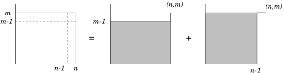
Figure 4: Graphical representation of the recursion relation (5.4)

Note that (5.5), unlike (5.4), involves generalized partition functions. However, the action of the translation group on the generalized partition function in (5.5) transforms them in ordinary partition functions by means of multiplication factor. We have

Theorem 5.4 (Action of the translation group)

For every $x\leq n^{\prime}$ and $y\leq m^{\prime}$

$$Z(n^{\prime},m^{\prime};n,m)=q^{2(x+y)(n-n^{\prime})}Z(n^{\prime}-x,m^{\prime}-y;n-x,m-y),$$ (5.6)

Proof: We first note that $Z(n^{\prime},m^{\prime};;n,m)$ is a polynomial in q that can be written as

$$Z(n^{\prime},m^{\prime};n,m)=q^{r}(1+a_{1}q^{2}+a_{2}q^{4}+...+a_{(m-m^{\prime})(n-n^{\prime})}q^{2(m-m^{\prime})(n-n^{\prime})})$$ (5.7)

where $r=[2(m^{\prime}+1)+2n^{\prime}](n-n^{\prime})+(n-n^{\prime})(n-n^{\prime}-1)$ is the minimum power of q among all the paths from $(n^{\prime},m^{\prime})$ to $(n,m)$, and the (positive) coefficients $a_{j}$ account for the multiplicity of the powers of $q^{2j}$. Namely given the box $B(n^{\prime},m^{\prime};n,m)$:

$$a_{j}\;=\;\#\{{\rm paths~{}in}~{}B(n^{\prime},m^{\prime};n,m)~{}|~{}A(p)=j\}.$$ (5.8)

If we perform a shift x in the horizontal direction and a shift y in the vertical direction, we obtain the translated partition function

$$Z(n^{\prime}-x,m^{\prime}-y;n-x,m-y)=q^{r^{\prime}}(1+a_{1}q^{2}+a_{2}q^{4}+...+a_{(m-m^{\prime})(n-n^{\prime})}q^{2(m-m^{\prime})(n-n^{\prime})})$$ (5.9)

where $r^{\prime}=[2(m^{\prime}-y+1)+2(n^{\prime}-x)](n-n^{\prime})+(n-n^{\prime})(n-n^{\prime}-1)$, and the polynomial inside the parenthesis on the right hand side of (5.9) is the same as in (5.7) because of the translation invariance of the area Hamiltonian in eq. (4.5). Consequently

$$Z(n^{\prime},m^{\prime};n,m)=q^{(r-r^{\prime})}Z(n^{\prime}-x,m^{\prime}-y;n-x,m-y),$$ (5.10)

which is just (5.6).

 

The application of the translation property (5.6) to the partition function in (5.5) provides a second independent relation between the partition functions containing only the nearest neighbors of the point $(n,m)$.

Lemma 5.5

The partition function satisfies

$$Z(n,m)=q^{2n}Z(n-1,m)+q^{2n}Z(n,m-1).$$ (5.11)

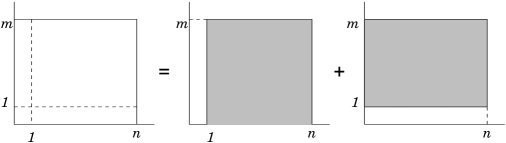
Figure 5: Graphical representation of the recursion relation (5.5)

Proof: Direct application of the translation property of (5.6) allows us to write the generalized partition functions in (5.5) in terms of ordinary partition functions

$$Z(1,0;n,m)=q^{2(n-1)}Z(n-1,m)\;\;\;\;{\rm and}\;\;\;\;Z(0,1;n,m)=q^{2n}Z(n,m-1)$$ (5.12)

Substituting (5.12) in (5.5) yields the lemma.
 

Remark 5.6

It is important to emphasize that the path integral formalism generated two independent relations between $Z(n,m)$, $Z(n-1,m)$ and $Z(n,m-1)$, namely (5.4) and (5.11), which are known as the q-Pascal identities for Gauss polynomials [6]. This fact is reminiscent of the situation found in the general theory of stochastic processes in which conditioning the process with respect to the initial or the final conditions provides two independent relations.

The independence of the two relations allow us to derive an explicitly expression for the partition function (5.7) as a product formula.

Theorem 5.7

The partition function $Z(n,m)$ is given by

$$Z(n,m)=q^{n(n+1)}~{}\frac{\prod_{i=1}^{n+m}(1-q^{2i})}{\prod_{i=1}^{n}(1-q^{2i})~{}\prod_{i=1}^{m}(1-q^{2i})}.$$ (5.13)

Proof: Solving (5.4) and (5.5) for $Z(n-1,m)$ and $Z(n,m-1)$ in terms of $Z(n,m)$ we get

$$\frac{Z(n-1,m)}{Z(n,m)}=q^{-2n}\frac{1-q^{2n}}{1-q^{2(n+m)}}\;\;\;\;{\rm and}\;\;\;\;\frac{Z(n,m-1)}{Z(n,m)}=\frac{1-q^{2m}}{1-q^{2(n+m)}}.$$ (5.14)

From (5.14) we obtain

$$\frac{Z(n-1,m-1)}{Z(n,m)}=q^{-2n}~{}\frac{(1-q^{2n})(1-q^{2m})}{(1-q^{2(L-1)})(1-q^{2L})}$$ (5.15)

Setting the initial condition $Z(0,0)=1$ yields the theorem.

 

Lemma 5.8

For $v\leq n$, $w\leq m$, the partition function $Z(n-v,m-w)$ satisfies

$$Z(n-v,m-w)\leq q^{-2nv+v(v-1)}~{}Z(n,m).$$ (5.16)

Proof: Starting from (5.15) and successively applying the first of the recursion relations (5.14) v times, we obtain

$$Z(n-v,m-1)=K_{v-1}L_{v-2}...L_{0}Z(n,m)$$ (5.17)

where, according to (5.14) and (5.15), we define

$$K_{j}=q^{-2(n-j)}~{}\frac{(1-q^{2(n-j)})(1-q^{2m})}{(1-q^{2(n-j+m-1)})(1-q^{2(n-j+m)})}\;\;\;\;{\rm and}\;\;\;\;L_{j}=q^{-2(n-j)}\frac{1-q^{2(n-j)}}{1-q^{2(n-j+m)}}.$$

Now, successively applying the second of the recursion relations (5.14) w times, we obtain

$$Z(n-v,m-w)=M_{w-1}...M_{1}Z(n,m)$$ (5.18)

where

$$M_{j}=\frac{1-q^{2(m-j)}}{1-q^{2(n+m-j)}}$$

Combining (5.17) and (5.18) gives

$$\frac{Z(n-v,m-w)}{Z(n,m)}\leq\prod_{j=0}^{v-1}q^{-2(n-j)}$$ (5.19)

and the theorem follows.

 

6. Probability Estimates

In this section we show how to bound the correlation functions for the quantum model through bounds on the path integral model correlations functions. The probability that a given spin, or a set of spins, are up or down can be expressed as sums of probabilities that a path goes through a given, or many, bonds.
The path integral representation provides a remarkable pictorial interpretation of these probabilities which allows us to obtain the estimates in an elementary way by efficiently exploiting the action of the translation group.
Our first result is the

Theorem 6.1

The probability that a path from the origin to $(n,m)$ pass through the point $(x,y)$ is given by

$$P_{n,m}(x,y)=q^{2(x+y)(n-x)}\frac{Z(x,y)Z(n-x,m-y)}{Z(n,m)}.$$ (6.1)

Proof: By the one-point correlation function (2.3) we have

$$P_{n,m}(x,y)=\frac{Z(n,m\mid x,y)}{Z(n,m)},$$ (6.2)

where $Z(n,m\mid x,y)$ is the number of paths from the origin to $(n,m)$ passing through the point $(x,y)$. By Theorem 4.1 we also have

$$Z(n,m\mid x,y)=Z(x,y)Z(x,y;n,m).$$ (6.3)

Now we use the translation property (5.6) to shift $Z(x,y;n,m)$. We obtain

$$Z(x,y;n,m)=q^{2(x+y)(n-x)}Z(n-x,m-y).$$ (6.4)

Substituting (6.4) in (6.2) yields the Theorem.

 

As to the probability that a path goes through a particular bond, we have the following estimates (which is useful for $x\geq n$)

Theorem 6.2

Considering the quantity

$$P(S^{z}_{x}=-1):=\frac{\langle\psi(n,m)\mid(1/2-S^{z}_{x})~{}\psi(n,m)\rangle}{\|\psi(n,m)\|^{2}}\;,$$ (6.5)

we have that

$$P_{n,m}(S^{z}_{x}=-1)\;=\;\sum_{j=x-m}^{n}P_{n,m}(j-1,x-j;j,x-j)\;$$ (6.6)

and the following bound holds

$$P_{n,m}(S^{z}_{x}=-1)\leq q^{2(x-n)}\frac{1-q^{2n}}{1-q^{2(n+m)}}.$$ (6.7)

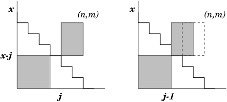
Figure 6: The paths in which the $x^{th}$ spin is down are contained in the two shaded areas in the diagram. To obtain the probability (6.9) we shift the upper box $B(j,x-j;n,m)$ one unit to the left and sum along the line x.

Remark 6.3

We have seen in Section 4 that the one-dimensional XXZ model and its ground states are invariant under the combined spin flip and left-right symmetries. This fact is implies the property

$$P_{n,m}(S_{x}^{z}=-1)=P_{m,n}(S_{L-x+1}^{z}=+1)\;,$$ (6.8)

In this way the properties that we are proving for $x\geq n$ can be transformed in the similar ones for $x\leq n$.

Proof: To obtain the probability that the $x^{th}$ spins is down, we have to sum the probabilities that the paths from $(0,0)$ to $(n,m)$ go horizontally through the diagonal line in which the sum of the coordinates is x because each horizontal bond in the path represent a down spin.
The graphical representation of this probability is shown in Fig 6 for $x\geq n$, $x\geq m$, and $x<n+m$. In this case, the $x^{th}$ step has to be taken in the horizontal direction. Then we have

$$P_{n,m}(S_{x}=-1)=\sum_{j=x-m}^{n}P_{n,m}(j-1,x-j;j,x-j)$$ (6.9)

where $P_{n,m}(j-1,x-j;j,x-j)$ is the probability that the path goes through the bond $(j-1,x-j)\rightarrow(j,x-j)$ is given by

$$P_{n,m}(j-1,x-j;j,x-j)=q^{2x}\frac{Z(j-1,x-j)Z(j,x-j;n,m)}{Z(n,m)}.$$ (6.10)

We see that each $P_{n,m}(j-1,x-j;j,x-j)$ is represented by a box from the origin to the tip of a horizontal bond on the sphere of radius x, connected to another box from the tip of the horizontal bond to the final point $(n,m)$.
A bound on $P_{n,m}(j-1,x-j;j,x-j)$ is the result of an operation we perform on Fig. 6, by shifting the upper box in the figure one unit to the left in the horizontal direction, as indicated. This is the same as making an equal shift on $Z(j,x-j;n,m)$. By the translation property (5.6), we have

$$Z(j,x-j;n,m)=q^{2(n-j)}Z(j-1,x-j;n-1,m).$$ (6.11)

We thus get

$$P_{n,m}(S_{x}=-1)=q^{2x}~{}\sum_{j=x-m}^{n}\frac{Z(j-1,x-j)Z(j-1,x-j;n-1,m)}{Z(n,m)}~{}q^{2(n-j)}.$$ (6.12)

The easy bound follows immediately

$$P_{n,m}(S_{x}=-1)\leq q^{2x}~{}\sum_{j=1}^{x}\frac{Z(j-1,x-j)Z(j-1,x-j;n-1,m)}{Z(n,m)},$$ (6.13)

and, by Theorem 4.1, the summation over j is nothing more than the partition function $Z(n-1,m)$.
Thus we get

$$P_{n,m}(S_{x}=-1)\leq q^{2x}~{}\frac{Z(n-1,m)}{Z(n,m)}.$$ (6.14)

We have worked out the ratio ${Z(n-1,m)}/{Z(n,m)}$ in Section 4. The substituting of formula (5.14) of that section in (6.14) gives the theorem.

 

The same reasoning with minor changes leads to the estimates for the probability that the $x^{th}$ spin is up. We have

Theorem 6.4

$$P_{n,m}(S^{z}_{x}=+1)\leq\frac{1-q^{2m}}{1-q^{2(n+m)}}.$$ (6.15)

Proof: As depicted in Fig.7, also for $x\geq n$, $x\geq m$ and $x\leq n+m$, we have

$$P_{n,m}(S_{x}=+1)=\sum_{j=x-m}^{n}P_{n,m}(j,x-j-1;j,x-j)$$ (6.16)

where $P_{n,m}(j,x-j-1;j,x-j)$ is the probability that the path goes through the bond $(j,x-j-1)\rightarrow(j,x-j)$ is given by

$$P_{n,m}(j,x-j-1;j,x-j)=\frac{Z(j,x-j-1)Z(j,x-j;n,m)}{Z(n,m)}.$$ (6.17)

By applying the translation property (5.6) to $Z(j,x-j;n,m)$ to shift it one unit down in the vertical direction, we get

$$Z(j,x-j;n,m)=q^{2(n-j)}Z(j,x-j-1;n,m-1).$$ (6.18)

Substituting the above relation in (6.16) gives

$$P_{n,m}(S_{x}=+1)\leq\sum_{j=x-m}^{n}\frac{Z(j,x-j-1)Z(j,x-j-1;n,m-1)}{Z(n,m)}=\frac{Z(n,m-1)}{Z(m,n)}.$$ (6.19)

By inserting (5.14) into the above expression gives the theorem.

 

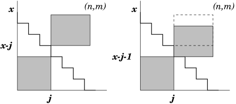
Figure 7: To obtain the probability (6.16) we shift the upper box down one unit and sum along the line x.

Finally, we have to consider the probability that adjacent spins are opposite. We suppose that the $x^{th}$ spins is down and the $(x+1)^{th}$ spins is up. We prove that

Theorem 6.5

$$P_{n,m}(S_{x}^{z}=-1,S_{x+1}^{z}=+1)\leq q^{2(x-n)}\frac{1-q^{2m}}{1-q^{2n}}\frac{1-q^{2L}}{1-q^{2(L-1)}}$$ (6.20)

Proof: For $x\geq n$, $x\geq m$ and $x<n+m$, we have

$$P_{n,m}(S_{x}^{z}=-1,S_{x+1}^{z}=+1)=\frac{q^{2x}}{Z(n,m)}\sum_{j=x-m}^{n}Z(j-1,x-j)~{}Z(j,x-j+1;n,m)$$ (6.21)

By performing a translation along both the horizontal and vertical direction by one unit, as in Fig. 8, we bring the origin of $Z(j,x-j+1;n,m)$ to the point $(j-1,x-j)$, thus obtaining

$$Z(j,x-j+1;n,m)=q^{4(n-j)}Z(j-1,x-j;n-1,m-1).$$ (6.22)

Substitution in (6.21) yields

$$P_{n,m}(S_{x}^{z}=-1,S_{x+1}^{z}=+1) \leq q^{2x}\sum_{j=x-m}^{n}\frac{Z(j-1,x-j)Z(j-1,x-j;n-1,m-1)}{Z(n,m)}$$ (6.23)

$$= q^{2x}\frac{Z(n-1,m-1)}{Z(n,m)}$$

and the theorem follows from (5.15).

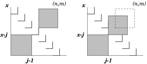
Figure 8: To obtain the probability (6.21) we shift the upper box to the left and down by one unit and sum along the line x.

7. Multi-Point Correlation Functions

We now extend the analysis of the previous section to include the probability that a string of r spins at positions $x_{1},x_{2},\cdots,x_{r}$ has a given configuration of up or down spins.
Let us consider multi-point correlation functions as given in the definitions (2.5) and (2.6), and paths from the origin to $(n,m)$ that cross successive spheres on the lattice of radius $x_{1},x_{2}\cdots,x_{r}$. We take the case in which $x_{j}>n,m$ and $x_{j}\leq n+m$ for $j=1,2,\cdots,r$.
We denote by $P_{n,m}(S_{x_{1}}^{z}=\sigma_{1},\cdots S_{x_{r}}^{z}=\sigma_{r})$ the probability that the spins at position $x_{1},x_{2}\cdots,x_{r}$ have a configuration $\sigma_{1},\sigma_{2},\cdots,\sigma_{r}$, with $\sigma_{j}=\pm 1$ for $j=1,2,\cdots,r$. Then

$$P(S_{x_{1}}^{z}=\sigma_{1}, \cdots S_{x_{r}}^{z}=\sigma_{r})=\frac{1}{Z(n,m)}\sum_{j_{1}=x_{1}-m}^{n}F(j_{1})~{}q^{2x_{1}(1-\bar{\alpha}_{1})}\;\;\;\;\;\;\;$$

$$\sum_{j_{2}=j_{1}}^{\Delta x_{2}+t_{1}}\cdots\sum_{j_{r-1}=j_{r-2}}^{\Delta x_{r-1}+t_{r-2}}~{}\sum_{j_{r}=j_{r-1}}^{n}~{}\left(\prod_{k=2}^{r}F(j_{k-1},j_{k})~{}q^{2x_{k}(1-\bar{\alpha}_{k})}\right)F(j_{r})$$

where have simplified the notation for the partition functions by denoting

$$F(j_{1})=Z(j_{1}-1,x_{1}-j_{1}),\;\;\;{\rm and}\;\;\;F(j_{r})=Z(j_{r}-\bar{\alpha}_{r},x_{r}-j_{r}+\bar{\alpha}_{r};n,m),$$ (7.2)

and

$$F(j_{k-1},j_{k})=Z(j_{k-1}-\bar{\alpha}_{k-1},x_{k-1}-j_{k-1}+\bar{\alpha}_{k-1};j_{k}-1,x_{k}-j_{k}).$$ (7.3)

We have also introduced the new variables $\bar{\alpha}_{k}=1-\alpha_{k}$, $t_{k}=j_{k}-\bar{\alpha}_{k}$ and $\Delta=x_{k}-x_{k-1}$.
The main result of this section is the following.

Theorem 7.1 (Exponential bounds on the correlations)

Let $v=\sum_{j=1}^{r}\alpha_{j}$ be the number of down spin on the observable set $\alpha_{1},\cdots,\alpha_{r}$, and let $d_{k}=(x_{k}-n)\alpha_{k}$ be the distances of a down spin from the point of coordinate $n$ (distance to the interface). Then the following bound holds

$$P(S_{x_{1}}^{z}=\sigma_{1},\cdots S_{x_{r}}^{z}=\sigma_{r})\leq q^{v(v-1)+2\sum_{k=1}^{r}d_{k}}\;.$$ (7.4)

This result extends (and reduce to in the case r=2 with up and down spin) the eq. (6.20).

Proof: We now use the translation property to first shift partition function in the last box $B(j_{r}-\bar{\alpha}_{r},x_{r}-j_{r}+\bar{\alpha}_{r};n,m)$ in (7.3) one unit to left (when $\bar{\alpha}_{k}=0$) or down (when $\bar{\alpha}_{k}=1$). We get

$$Z(j_{r}-\bar{\alpha}_{r},x_{r}-j_{r}+\bar{\alpha}_{r};n,m)=q^{2(n-j_{r}+\bar{\alpha}_{r})}~{}Z(j_{r}-1,x_{r}-1;n-(1-\bar{\alpha}_{r}),m-\bar{\alpha}_{r})$$ (7.5)

Next we estimate the factor of q above by one before substituting (7.5) in (), and we also factorize out all the bond weights $2x_{k}(1-\bar{\alpha}_{k})$, thus obtaining the bound

$$P(S_{x_{1}}^{z}=\sigma_{1}, \cdots S_{x_{r}}^{z}=\sigma_{r})\leq q^{2\sum_{k=1}^{r}x_{k}(1-\bar{\alpha}_{k})}~{}\frac{1}{Z(n,m)}\sum_{j_{1}=x_{1}-m}^{n}Z(j_{1}-1,x_{1}-j_{1})$$

$$\sum_{j_{2}=j_{1}}^{\Delta x_{2}+t_{1}}\cdots\sum_{j_{r-1}=j_{r-2}}^{\Delta x_{r-1}+t_{r-2}}~{}\left(\prod_{k=2}^{r-1}F(j_{k-1},j_{k})~{}\right)Z_{r-1}(n-(1-\bar{\alpha}_{r}),m-\bar{\alpha}_{r})$$

where we have observed that by carrying out the summation over $j_{r}$ we obtain the partition function

$$Z_{r-1}(n-(1-\bar{\alpha}_{r}),m-\bar{\alpha}_{r}) = \sum_{j_{r}=j_{r-1}}^{n}Z(j_{r-1}-\bar{\alpha}_{r-1},x_{r-1}-j_{r-1}+\bar{\alpha}_{r-1};j_{r}-1,x_{r}-j_{r})$$ (7.7)

$$\;\;\;\;Z(j_{r}-1,x_{r}-1;n-(1-\bar{\alpha}_{r}),m-\bar{\alpha}_{r}).$$

From here we will need to repeat this procedure of performing shifts of one unit down or to the left in succession to the partition functions in (). After each step the resulting partition function obtained is changed according to the number of shifts we have performed. At the end, we get

$$P(S_{x_{1}}^{z}=\sigma_{1},\cdots S_{x_{r}}^{z}=\sigma_{r})\leq q^{2\sum_{k=1}^{r}x_{k}\alpha_{k}}~{}\frac{Z(n-\sum_{k=1}^{r}\alpha_{k},~{}m-\sum_{k=1}^{r}(1-\alpha_{k}))}{Z(n,m)}.$$ (7.8)

Substituting (5.16) in (7.8), with $v=\sum_{k=1}^{r}\alpha_{k}$ yields the theorem.

 

Theorem 7.1 can be used to study the fluctuations around the interface. In combination with the conservation of the third component of the spin, the bound implies that fluctuations are strongly correlated. In order to illustrate this we consider the total third component of the spin on an interval centered on the interface: let $N$ and $L$ be even positive numbers, $L\leq N$, and consider the state $\psi(N/2,N/2)$, and let $\langle\cdot\rangle_{N}$ denote the expectation in this state. Define $F_{L}$ by

$$F_{L}=\sum_{x=(N-L)/2+1}^{(N+L)/2}S^{z}_{x}$$ (7.9)

We will also need the total third component of the spin in the complement of the interval $[(N-L)/2+1,(N+L)/2]$, defined by

$$F_{L}^{c}=\sum_{x\not\in[(N-L)/2+1,(N+L)/2]}S^{z}_{x}$$

Then, for all $L\leq N$,

$$\langle F_{L}\rangle_{N}=0$$

as a consequence of the symmetry properties given in Theorem 4.3.

Theorem 7.2

$$\lim_{L\to\infty}\lim_{N\to\infty}Prob_{N}(F_{L}=l)=\delta_{l,0}$$ (7.10)

Proof: The distribution of $F_{L}$, and, hence, its variance, can be estimated by first noting that

$$Prob_{N}(F_{L}=l)=Prob_{N}(F^{c}_{L}=-l)=Prob_{N}(F^{c}_{L}=l)$$

and further that

$$Prob_{N}(F^{c}_{L}=l)\leq Prob_{N}(\mbox{there are at least $l$ down spins in $[(N+L)/2+1,N]$})$$

By summing the bound of Theorem 7.1 over all numbers $r\geq l$ of down spins to the right of $(N+L)/2$, and possible positions $x_{1},\ldots,x_{r}$, we obtain the following bound:

$$Prob_{N}(\mbox{there are at least $l$ down spins in $[(N+L)/2+1,N]$})$$

$$\leq \sum_{r=l}^{(N-L)/2}\sum_{(N+L)/2<x_{1}<\cdots<x_{r}\leq N}q^{r(r-1)+2\sum_{k=1}^{r}(x_{k}-N/2)}\;\;\;\;\;\;\;\;\;\;\;\;$$

$$\leq \sum_{r=l}^{\infty}\frac{q^{r(r-1)}}{r!}\left[\sum_{x=L/2+1}^{\infty}q^{2x}\right]^{r}$$

$$\leq \sum_{r=l}^{\infty}\frac{q^{r(r-1)}}{r!}\left[\frac{q^{L+2}}{1-q^{2}}\right]^{r}$$

$$\leq q^{l(l-1)}\frac{1}{l!}\left[\frac{q^{L+1}}{1-q^{2}}\right]^{l}\exp[q^{L+3}/(1-q^{2})]\leq C(q)q^{l^{2}+Ll}$$

where $C(q)$ is a constant depending only on $q$. From this bound it is clear that

$$\lim_{L\to\infty}\mathop{\overline{\rm lim}}_{N\to\infty}Prob_{N}(F_{L}=l)=\delta_{l,0}$$ (7.11)

As it has been shown in [3] that the limit $N\to\infty$ exists, this concludes the proof.

 

8. Higher Dimensions

The path integral formulation we have introduced provides an efficient way to bound correlation functions of the quantum XXZ model in one dimension. For higher dimensions it is known that the state with n spins down in d dimensions is given by [2]

$$\psi(n,m)=\sum_{\alpha_{x}}\left\{\prod_{x}q^{\alpha_{x}|x|}\right\}\mid\{\alpha_{x}\}\rangle.$$ (8.1)

where $|x|$ is the $L_{1}$ norm of the vector $x$.
We consider a two-dimensional spin system in order to illustrate how to relate the property of the model in higher dimensions to those of a one dimensional system.
Since we are free to choose the orientation of the physical spin system, we prefer to dispose the spins along M diagonal lines with each diagonal having the same number N of spins, as in the first diagram of Fig. 9. The weights assigned to the bonds in the corresponding path representation follow the diagonal pattern shown in the second diagram of Fig. 9. The analytic expression for the weight of a bond in this case is

$$w(b)=\left\{\begin{array}[]{ll}x+y\;\;\;{\rm any~{}horizontal~{}bond~{}ending~{}at}~{}(x,y)\\ 1\;\;\;\;\;\;\;\;\;\;\;{\rm any~{}vertical~{}bond}\end{array}\right.$$ (8.2)

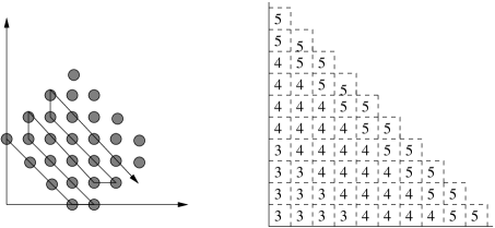
Figure 9: The spin system in any dimension can be put in correspondence with a one-dimensional spins system by using the Cantor diagonal procedure as indicated in the diagram for the two-dimensional case.

Our result is based on eq. (5.6) and shows in detail the mechanism of dimensional reduction which underlines the methods used to prove to absence of gap for interface excitations in $d=3$ [7].
The main result of this section is the following theorem.

Theorem 8.1

Consider a two-dimensional system shown in Fig.10a, having sizes $N$ and $M$. Let ${\cal K}$ be the set of $m$ non-negative integers $\{k_{i}\}$ such that $\sum_{i=0}^{m}ik_{i}=k$ and $\sum_{i=0}^{m}k_{i}=N$. The norm of the ground state of the two-dimensional system with $k$ spins down, $Z_{2d}(k,NM-k)$, is given by

$$Z_{2d}(k,NM-k)=q^{2(N-1)k}\sum_{\{k_{i}\}\in{\cal K}}\frac{N!}{k_{0}!k_{1}!...k_{m}!}\prod_{i=1}^{m}\left\{Z(j,M-j)\right\}^{k_{j}}\;.$$ (8.3)

where $Z(j,M-j)$ are the partition functions of the one-dimensional model.

Examples. To illustrate the theorem let us calculate the two-dimensional partition function for a system of 9 spins with $N=3,M=3$. We take $k=3$. In this case, there are three set of allowed values of $(k_{0},k_{1},k_{2},k_{3})$. They are $(2,0,0,1)$, $(1,1,1,0)$ and $(0,3,0,0)$. Thus we obtain

$$Z_{2d}(3,6)=q^{12}\left\{{Z(1,2)}^{3}+6Z(1,2)Z(2,1)+3Z(3,0)\right\}$$ (8.4)

When $n=4,m=5$, the following are the sets of allowed k values are $(2,0,0,1)$, $(1,1,1,0)$ and $(0,3,0,0)$. We get

$$Z_{2d}(4,5)=q^{16}\left\{6Z(1,2)Z(3,0)+3{Z(2,1)}^{2}+3Z(3,0)\right\}$$ (8.5)

Proof: Because of the periodic pattern of the weights in path space, the grand-canonical partition function in two-dimensions is given by

$$Z_{GC}^{2d}=\prod_{j=N}^{N+M-1}(1+zq^{2j})^{N}=\sum_{k=0}^{NM}z^{k}Z_{2d}(k,NM-k),$$ (8.6)

where $Z_{2d}(k,NM-k)$ is the canonical partition function in two-dimensions.
The product formula in (8.6) can also be written in terms of the generalized canonical partition functions of the one-dimensional system. By interchanging the $N$-th power with the product in eq. (8.6) we get

$$\prod_{j=N}^{N+M-1}(1+zq^{2j})^{N}=\left\{\sum_{l=0}^{M}z^{l}Z_{1d}(N-1,0;N-1+l,M-l)\right\}^{N}$$ (8.7)

where the generalized partition functions have initial points $(N-1,0)$ in order to account of the proper relation between the weights of the corresponding one-dimensional and two-dimensional systems as we have defined them.
Now we use the translation property (5.6) to shift the generalized partition functions in (8.7) to the origin. In doing this we obtain a multiplicative factor depending on the first set of weights of the two-dimensional system:

$$Z_{1d}(N-1,0;N-1+l,M-l)=q^{2(N-1)l}Z_{1d}(l,M-l)$$ (8.8)

Substituting the above expression into (8.7) we get

$$\prod_{j=N}^{N+M-1}(1+zq^{2j})^{N}=\left\{\sum_{l=0}^{M}z^{l}q^{2(N-1)l}Z_{1d}(l,M-l)\right\}^{N}.$$ (8.9)

Equating (8.9) to the expression on the right hand side of (8.6) yields

$$\sum_{k=0}^{NM}z^{k}Z_{2d}(k,NM-k)=\left\{\sum_{l=0}^{M}z^{l}q^{2(N-1)l}Z_{1d}(l,M-l)\right\}^{N}$$ (8.10)

Since the equality in (8.10) holds term by term in powers of z, we express the two-dimensional partition function as a sum of one-dimensional partition functions given by

$$Z_{2d}(k,NM-k)=q^{2(N-1)k}\sum_{k_{0},k_{1},k_{2},...k_{m}}\frac{N!}{k_{0}!k_{1}!...k_{m}!}\prod_{i=1}^{m}\left\{Z_{1d}(j,M-j)\right\}^{k_{j}}$$ (8.11)

where the sum runs over the values of k with the restrictions $k_{1}+2k_{2}+3k_{3}+...+mk_{m}=k$, and $k_{0}=N-\sum_{i=1}^{m}k_{i}$.

 

Acknowledgments P.C. thanks G. Kuperberg for several interesting discussions on counting and q-counting problems. O.B. was supported by FAPESP under grant 97/14430-2. B.N. acknowledges partial support by NSF under grant DMS-9706599.

References

[1]
M. Aizenman and B. Nachtergaele, Geometric Aspects of Quantum Spin
States, Commun. Math. Phys., 164 (1994) 17–63.
[2]
F. C. Alcaraz, S. R. Salinas, W. F. Wreszinski, Anisotropic
Ferromagnetic Quantum Domains, Phys. Rev. Lett.75
(1995) 930.
[3] C. T. Gottstein, R.F. Werner, Ground states of the
q-deformed Heisenberg ferromagnet, preprint archived as
cond-mat/9501123
[4] T. Koma, B. Nachtergaele,
Low-lying spectrum of quantum interfaces, Abstracts of the
AMS, 17 (1996) 146, and unpublished notes.
[5]
F.H.L. Essler, H. Frahm, A. Its, and V.E. Korepin,
Integro-difference equation for a correlation function of the
spin- Heisenberg XXZ chain, Nucl. Phys.446B (1995) 448–460.
[6]
C. Kassel,
Quantum Groups, Graduate Texts in Mathematics vol. 155,
Springer Verlag, New York, 1995.
[7] O. Bolina, P. Contucci, B. Nachtergaele, and S. Starr,
Finite volume excitations of the 111 interface in the quantum
XXZ model, in preparation.