Geometry, stochastic calculus and quantum fields in a non-commutative space-time

Abstract

The algebras of non-relativistic and of classical mechanics are unstable algebraic structures. Their deformation towards stable structures leads, respectively, to relativity and to quantum mechanics. Likewise, the combined relativistic quantum mechanics algebra is also unstable. Its stabilization requires the non-commutativity of the space-time coordinates and the existence of a fundamental length constant.

The new relativistic quantum mechanics algebra has important consequences on the geometry of space-time, on quantum stochastic calculus and on the construction of quantum fields. Some of these effects are studied in this paper.

1 The instability of relativistic quantum mechanics and a fundamental length

Physical models and theories are mere approximations to Nature and the physical constants can never be known with absolute precision. Therefore, if a fine tuning of the parameters is needed to reproduce some particular phenomenon, it is probable that the model is basically unsound and that its other predictions are unreliable. A wider range of validity is expected for theories that do not change in a qualitative manner for a small change of parameters. Such theories are called stable or rigid.

A mathematical structure is said to be stable (or rigid) for a class of deformations if any deformation in this class leads to an equivalent (isomorphic) structure. The idea of stability of structures provides a guiding principle to test either the validity or the need for generalization of a physical theory. Namely, if the mathematical structure of a given theory turns out to be unstable, one might just as well deform it, until one falls into a stable one, which has a good chance of being a generalization of wider validity.

The stable-model point of view had a large impact in the field of non-linear dynamics, where it led to the notion of structural stability[1][2]. As emphasized by Flato[3] and Faddeev[4] the same pattern seems to occur in the fundamental theories of Nature. In fact, the two most important physical revolutions of this century, namely the passage from non-relativistic to relativistic and from classical to quantum mechanics, may be interpreted as the transition from two unstable theories to two stable ones. In the non-relativistic mechanics case, one notices that the second cohomology group of the homogeneous Galileo group does not vanish and the corresponding algebra has a deformation that leads to the Lorentz algebra which, being semisimple, is stable. In turn, the transition from classical to quantum mechanics may be regarded as a deformation of the unstable Poisson algebra of phase-space functions to the stable Moyal-Vey algebra[5]. I will refer to these two stabilizing deformations as the $\frac{1}{c}$-deformation and the $\hbar$-deformation. The deformed algebras are all equivalent for non-zero values of $\frac{1}{c}$ and $\hbar$. Hence, relativistic mechanics and quantum mechanics may be derived from the conditions for stability of their algebras, but the exact values of the deformation parameters cannot be fixed by purely algebraic considerations. Instead, the deformation parameters are fundamental constants to be obtained from experiment. In this sense not only is deformation theory the theory of stable theories, it is also the theory that identifies the fundamental constants.

A review of deformation theory and of the transition from non-relativistic to relativistic and from classical to quantum mechanics as the deformation-stabilization of two unstable theories is contained in Ref.[6]. Also, it is shown there that both deformations may be studied in the context of finite-dimensional Lie algebras, which is simpler than the usual treatment of quantum mechanics as a deformation of an infinite-dimensional algebra of functions. The algebra that results from the $\frac{1}{c}$-deformation is the Lorentz algebra and the one coming from the $\hbar$-deformation is the Heisenberg algebra. A simple fact in this construction, which however has non-trivial consequences, is that, to have both constructions in a finite-dimensional algebra setting, it is essential to include the coordinates as basic operators in the defining (kinematical) algebra of relativistic quantum mechanics. The full algebra of relativistic quantum mechanics will then contain the Lorentz algebra $\{M_{\mu\nu}\}$, the Heisenberg algebra for the momenta and space-time coordinates $\{p_{\mu},x_{\nu}\}$ in Minkowski space and also the commutators that define the vector nature (under the Lorentz group) of $p_{\mu}$ and $x_{\nu}$, namely

$$\begin{array}[]{rll}[M_{\mu\nu},M_{\rho\sigma}]&=&i(M_{\mu\sigma}\eta_{\nu\rho}+M_{\nu\rho}\eta_{\mu\sigma}-M_{\nu\sigma}\eta_{\mu\rho}-M_{\mu\rho}\eta_{\nu\sigma})\\ [M_{\mu\nu},p_{\lambda}]&=&i(p_{\mu}\eta_{\nu\lambda}-p_{\nu}\eta_{\mu\lambda})\\ [M_{\mu\nu},x_{\lambda}]&=&i(x_{\mu}\eta_{\nu\lambda}-x_{\nu}\eta_{\mu\lambda})\\ [p_{\mu},p_{\nu}]&=&0\\ [x_{\mu},x_{\nu}]&=&0\\ [p_{\mu},x_{\nu}]&=&i\eta_{\mu\nu}\Im\end{array}$$ (1)

with $\eta_{\mu\nu}=(1,-1,-1,-1)$, $c=\hbar=1$ and $\Im$ a unit that commutes with all the other operators.

One knows that the Lorentz algebra, being semi-simple, is stable and that each one of the 2-dimensional Heisenberg algebras $\{p_{\mu},x_{\nu}\}$ is also stable in the non-linear sense discussed in Ref.[6]. When the two algebras are combined through the covariance commutators, the natural question to ask is whether the whole algebra is stable or whether there are any non-trivial deformations. The answer[6] is that the algebra $\Re_{0}=\{M_{\mu\nu},p_{\mu},x_{\mu},\Im\}$ defined by Eqs.(1) is not stable. This is shown by exhibiting a 2-parameter $(\ell,R)$-deformation of $\Re_{0}$ to a simple algebra $\Re_{\ell,R}$ which itself is stable, namely

$$\begin{array}[]{rcl}[M_{\mu\nu},M_{\rho\sigma}]&=&i(M_{\mu\sigma}\eta_{\nu\rho}+M_{\nu\rho}\eta_{\mu\sigma}-M_{\nu\sigma}\eta_{\mu\rho}-M_{\mu\rho}\eta_{\nu\sigma})\\ [M_{\mu\nu},p_{\lambda}]&=&i(p_{\mu}\eta_{\nu\lambda}-p_{\nu}\eta_{\mu\lambda})\\ [M_{\mu\nu},x_{\lambda}]&=&i(x_{\mu}\eta_{\nu\lambda}-x_{\nu}\eta_{\mu\lambda})\\ [p_{\mu},p_{\nu}]&=&-i\frac{\epsilon^{{}^{\prime}}}{R^{2}}M_{\mu\nu}\\ [x_{\mu},x_{\nu}]&=&-i\epsilon\ell^{2}M_{\mu\nu}\\ [p_{\mu},x_{\nu}]&=&i\eta_{\mu\nu}\Im\\ [p_{\mu},\Im]&=&-i\frac{\epsilon^{{}^{\prime}}}{R^{2}}x_{\mu}\\ [x_{\mu},\Im]&=&i\epsilon\ell^{2}p_{\mu}\\ [M_{\mu\nu},\Im]&=&0\end{array}$$ (2)

$\epsilon$ and $\epsilon^{{}^{\prime}}$ being $\pm$ signs. The stable algebra $\Re_{\ell,R}$ to which $\Re_{0}$ has been deformed is the algebra of the 6-dimensional pseudo-orthogonal group with metric $\eta_{aa}=(1,-1,-1,-1,\epsilon^{{}^{\prime}},\epsilon)$ and commutation relations

$$[M_{ab},M_{cd}]=i(-M_{bd}\eta_{ac}-M_{ac}\eta_{bd}+M_{bc}\eta_{ad}+M_{ad}\eta_{bc})$$ (3)

the correspondence being established by

$$\begin{array}[]{lll}p_{\mu}&=&\frac{1}{R}M_{\mu 4}\\ x_{\mu}&=&\ell M_{\mu 5}\\ \Im&=&\frac{\ell}{R}M_{45}\end{array}$$ (4)

To understand the role of the deformation parameters consider first the Poincaré subalgebra $P=\{M_{\mu\nu},p_{\mu}\}$ of $\Re_{0}$. It is well known that already this subalgebra is not stable and may be deformed[3] [7] to the stable simple algebras of the De Sitter groups O(4,1) or O(3,2). This is the deformation that corresponds to the parameter $R$. This instability of the Poincaré algebra is however physically harmless and well understood. It simply means that flat space is an isolated point in the set of arbitrarily curved spaces. Faddeev[4] points out that Einstein’s theory of gravity may be interpreted as a deformation. This theory is based on curved pseudo Riemannian manifolds. Therefore, in the set of Riemannian manifolds, Minkowski space is an isolated point, whereas a generic Riemannian manifold is stable in the sense that in its neighborhood all spaces are curved. However, as long as the Poincaré group is used as the kinematical group of the tangent space to the space-time manifold, and not as a group of motions in the manifold itself, it is perfectly consistent to take $R\rightarrow\infty$ and this deformation goes away.

For the other deformation parameter ($\ell$) there is no reason to imagine that it should vanish, even in tangent space, if one insists on the stability paradigm as the guiding principle for theory construction. One is therefore led to $\Re_{\ell,\infty}$ as our candidate for a stable algebra of relativistic quantum mechanics in the tangent space. The main features are the non-commutativity of the $x_{\mu}$ coordinates and the fact that $\Im$, previously a trivial center of the Heisenberg algebra, becomes now a non-trivial operator. Two constants define this deformation. One is $\ell$, a fundamental length, the other the sign of $\epsilon$. The tangent space algebra $\Re_{\ell,\infty}$ would be the kinematical algebra appropriate for microphysics. For physics in the large, one might however use $\Re_{\ell,R}$ with (finite) $R^{2}$ related to the gravitational constant $G$.

The idea of modifying the algebra of the space-time components $x_{\mu}$ in such a way that they become non-commuting operators had already appeared several times in the physical literature. However, rather than being motivated (and forced) by stability considerations, the aim of those proposals was to endow space-time with a discrete structure, to be able, for example, to construct quantum fields free of ultraviolet divergences. Sometimes a non-zero commutator was simply postulated, some other times the motivation was the formulation of field theory in curved spaces. Although the algebra discussed above is so simple and appears in such a natural way in the context of deformation theory, it seems that, strangely, it differs in some way or another from the past proposals. In some schemes, for example, the coordinates were assumed to be the generators of rotations in a 5-dimensional space with constant negative curvature. This possibility was proposed long ago by Snyder[8] and the consequences of formulating field theories in such spaces were extensively studied by Kadishevsky and collaborators[9] [10]. The coordinate commutation relations $[x_{\mu},x_{\nu}]$ are identical to those in (2), however, because of the representation chosen for the momentum operators, the Heisenberg algebra is different and, in particular, $[p_{\mu},x_{\nu}]$ has non-diagonal terms. Banai[11] also proposed a specific non-zero commutator which only operates between time and space coordinates, breaking Lorentz invariance. Many other discussions exist concerning the emergence and the role of discrete or quantum space-time, which however, in general, do not specify a complete operator algebra[12] [13] [14] [15] [16] [17] [18] [19] [20] [21] [22] [23] [24] [25] [26].

In $\Re_{\ell,\infty}$, the fact that $\Im$ becomes a non-trivial operator changes the structure of the Heisenberg algebra. This has some consequences on the construction of the state spaces even for nonrelativistic quantum mechanics. This was partly discussed in Ref.[27]. Here the emphasis will be on the study of the geometric structure of space-time that follows from the $\Re_{\ell,\infty}$ algebra and on the nature of quantum fields. In particular the larger set of derivations that $\Re_{\ell,\infty}$ possesses has for gauge fields some important consequences that do not depend on the size of the parameter $\ell$ , but only on the fact that it is different from zero.

In Sect.2 one collects the basic facts about the non-commutative geometry of space-time which are implied by the algebra $\Re_{\ell,\infty}$. In particular, the role of the elementary sets of the geometry is clarified and a differential calculus developed. In a general non-commutative geometry setting [28], differential calculus cannot be developed through derivations, because for some algebras there is not enough derivations. Then, the non-commutative analog of the Dirac operator is used for this purpose. In the $\Re_{\ell,\infty}$ case, however, an approach through derivations is possible. This has the advantage of making the commutative limit ($\ell\rightarrow 0$) very transparent. Nevertheless, correspondence with the related Dirac operator approach is also established.

The representation theory of algebras is the basic tool to extract physical consequences from the non-commutative geometry. This is discussed at length in Sect.3. In the $\Re_{\ell,\infty}$ algebra, the usual Heisenberg algebras are replaced by the algebras of ISO(2) and ISO(1,1). A construction of a quantum stochastic calculus based on these algebras is sketched in the Appendix.

Integration in non-commutative space-time is discussed in Sect.4 and finally Sect.5 is dedicated to the construction of local quantum fields, the main emphasis being on the non-commutative geometry implications for gauge field interactions.

2 The noncommutative space-time geometry

Every geometrical property of an ordinary (commutative) manifold $M$ may be expressed as a property of the commutative $C^{*}$-algebra $C_{0}(M)$ of continuous functions on $M$ vanishing at infinity. For example, there is a one-to-one correspondence between the characters of $C_{0}(M)$ and the points of the manifold $M$, regular Borel measures on $M$ correspond to positive linear functionals on $C_{0}(M)$, complex vector bundles over $M$ are given by the finite projective modules over $C_{0}(M)$, etc. Similarly in non-commutative geometry one starts from a non-commutative $C^{*}$ -algebra and uses the same correspondence as in the commutative case to characterize the geometric properties of the non-commutative space[28][29].

In a general representation, the operators in $\Re_{\ell,\infty}$ are not bounded operators. However, once a representation of $\Re_{\ell,\infty}$ is obtained, there are standard ways to construct bounded operators from unbounded ones, in the universal enveloping algebra of $\Re_{\ell,\infty}$. For example,

$$\Gamma\rightarrow\exp(i\alpha\Gamma)$$ (5)

or

$$\Gamma\rightarrow\Gamma(1+\Gamma^{*}\Gamma)^{-\frac{1}{2}}$$ (6)

and one constructs from the latter, by norm-completion, the associated $C^{*}$-algebra. Therefore, for simplicity, the discussion of the representations may be carried out at the $\Re_{\ell,\infty}$ algebra level, even if the non-commutative space-time algebra is actually a $C^{*}$-algebra $C_{\Re}$ obtained by the restriction to the bounded operators in the universal enveloping algebra $U_{\Re}$ of $\Re_{\ell,\infty}$ and norm completion.

2.1 The elementary sets of the geometry. Commutative versus noncommutative space-time

In the commutative case, the elementary sets of the space-time manifold $M$ (the points with coordinates $x_{\mu}$) are in a one-to-one correspondence with the character representations of the algebra. In non-commutative case the elementary sets are the irreducible unitary representations of the algebra.

In $\Re_{\ell,\infty}$, the set $A_{M}=\{x_{\mu},M_{\mu\nu}\}$ is the minimal algebraically closed set that contains the space-time coordinate operators. It is therefore their representations that define the basic structure of non-commutative space-time. Therefore it is appropriate to compare the nature of the representations of the $A_{M}$ algebra for the commutative and the noncommutative cases. In the commutative case $A_{M}$ is a Poincaré algebra and in the noncommutative case it is a DeSitter algebra (of O(3,2) for $\epsilon=+1$ and of O(4,1) for $\epsilon=-1$). In the following, for definiteness, I will use $\epsilon=-1$. In the commutative case the elementary sets $T_{K}$ of the geometry are the spinless representations of the Poincaré group corresponding to fixed $x_{\mu}x^{\mu}$

$$T_{K}=\left\{x^{\mu}|(x^{0})^{2}-(x^{1})^{2}-(x^{2})^{2}-(x^{3})^{2}=K\right\}$$

From the physical point of view it makes sense to consider these (and not the points $x_{\mu}$) as the elementary sets of the geometry because each particular point $x_{\mu}$ in $T_{K}$ is just a particular aspect of the same event seen in different frames. In the noncommutative case the elementary sets are the representations of the DeSitter group which reduce to these Poincaré group representations in the $\ell\rightarrow 0$ limit.

The correspondence is made very clear by using the explicit representation of the operators of the $\Re_{\ell,\infty}$ algebra as differential operators in a 5-dimensional commutative manifold $M_{5}=\{\xi_{\mu}\}$ with metric $\eta_{aa}=(1,-1,-1,-1,\epsilon)$

$$\begin{array}[]{lll}M_{\mu\nu}&=&i(\xi_{\mu}\frac{\partial}{\partial\xi^{\nu}}-\xi_{\nu}\frac{\partial}{\partial\xi^{\mu}})\\ x_{\mu}&=&\xi_{\mu}+i\ell(\xi_{\mu}\frac{\partial}{\partial\xi^{4}}-\epsilon\xi^{4}\frac{\partial}{\partial\xi^{\mu}})\end{array}$$ (7)

In $M_{5}$ consider the family of hypersurfaces

$$\Gamma_{K}=\{\xi|(\xi^{0})^{2}-(\xi^{1})^{2}-(\xi^{2})^{2}-(\xi^{3})^{2}-(\xi^{4})^{2}=K\}$$

for $K\in(-\infty,\infty)$. For each fixed $K$, $\Gamma_{K}$ carries a representation of the DeSitter group (for $\epsilon=-1$). The intersection of each $\Gamma_{K}$ with any plane $\xi^{4}=c$ is a 3-dimensional hypersurface $T_{K+c^{2}}$ that corresponds to a spinless irreducible unitary representation of the Poincaré group. However, because of the $(\mu,4)-$rotations in the $x_{\mu}$ operator (Eq.(7)), it is $\Gamma_{K}$ that is irreducible for the $A_{M}$ algebra. Therefore the elementary sets of the commutative space-time geometry correspond to the $T_{K}$ sets and those of noncommutative space-time to the $\Gamma_{K}$ ${}^{{}^{\prime}}$s. It should however be clear the $T_{K}$ and $\Gamma_{K}$ sets are simply abstract representations of the irreducible representations of the algebra and their dimensionality should not be confused with the dimensionality of space-time. The manifold $M_{5}$ is simply the carrier of the representation of the non-commutative space-time algebra. Space-time is still defined by the same four $x_{\mu}$ operators operating on the elementary geometric sets. Fig.1 depicts the structure of the elementary sets with the $\Gamma_{K}$ ${}^{{}^{\prime}}$s, when intersected by the $\xi^{4}=1$ plane, generating the elementary sets of the pseudo-Euclidean (commutative) Minkowski geometry (and the intersection with the $\xi^{0}=0$ plane generating an Euclidean geometry).

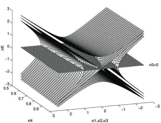
Figure 1: Representation of elementary sets in space-time geometry: commutative versus noncommutative

Although not changing the dimensionality of space-time, the $\Gamma_{K}$ sets, as compared to the $T_{K}$’s, have a richer group of motions and, in particular, a richer set of derivations, as will be seen below.

2.2 Derivations as vector fields and the differential algebra

A differential algebra may be defined either by duality from the derivations of the algebra when a sufficient number of derivations is available or directly from the triple $\left(H,\pi(C_{\Re}),D\right)$, where $\pi(C_{\Re})$ is a representation of the $C_{\Re}$ algebra in the Hilbert space $H$ and $D$ is the Dirac operator. In this latter case the commutator with the Dirac operator is used to obtain the one-forms. In the most general non-commutative framework[28] it is not always possible to use the derivations of the algebra to construct by duality the differential forms. In fact many algebras have no derivations at all. However when the algebra has enough derivations it is useful to consider them[30][31] because the correspondence of the non-commutative geometry notions to the classical ones becomes very clear. In our case it means to obtain the usual commutative geometry notions in the limit $\ell\rightarrow 0$. For this reason the construction through derivations will be used here and the correspondence to the Dirac commutator approach will be established later on.

Although not essential, the representation of the remaining operators of the $\Re_{\ell,\infty}$ algebra as differential operators on $M_{5}$ provides an intuitive interpretation of the derivations and is listed below

$$\begin{array}[]{lll}p_{\mu}&=&i\frac{\partial}{\partial\xi^{\mu}}\\ \Im&=&1+i\ell\frac{\partial}{\partial\xi^{4}}\end{array}$$ (8)

The derivations of the algebra play, as in the classical case, the role of vector fields. The derivations that are considered, to construct by duality the differential algebra, play only a subsidiary role in identifying the minimal extension needed when going from the commutative ($\ell=0$) to the non-commutative case ($\ell\neq 0$). In the end it is the resulting differential algebra which plays the central role.

The minimal algebraically closed subalgebra that contains the coordinate operators, $A_{M}=\left\{x_{\mu},M_{\mu\nu}\right\}$, being semisimple, it only has inner derivations. In particular because of the commutation relation $[p_{\mu},x_{\nu}]=i\eta_{\mu\nu}\Im$ and the non-triviality of the $\Im$ operator, the derivations that correspond to the momentum operator are not contained in the set of derivations of the enveloping algebra of $A_{M}$ (Der$\{U_{A_{M}}\}$). Therefore, to obtain enough derivations, one should consider the full algebra $\Re_{\ell,\infty}$ and its generalized enveloping algebra $U_{\Re}$, to which a unit and, for later convenience, the inverse of $\Im$, are also added.

$$U_{\Re}=\{x_{\mu},M_{\mu\nu},p_{\mu},\Im,\Im^{-1},1\}$$ (9)

The derivations of $\Re_{\ell,\infty}$ are the inner derivations plus a dilation ${\cal D}$ which acts on the generators as follows

$$\begin{array}[]{lllll}[{\cal D},P_{\mu}]&=&P_{\mu}&&\\ [{\cal D},\Im]&=&\Im&&\\ [{\cal D},M_{\mu\nu}]&=&[{\cal D},x_{\mu}]&=&0\end{array}$$ (10)

This may be computed directly or, alternatively, by embedding $\Re_{\ell,\infty}$ into O(2,5), noticing that this algebra has only inner derivations and selecting those that operate inside $\Re_{\ell,\infty}$. Therefore

$$\textnormal{Der}\{\Re_{\ell,\infty}\}=\{x_{\mu},M_{\mu\nu},p_{\mu},\Im,{\cal D}\}$$

Any element of the form $a\delta$, where $a\in U_{\Re}$ and $\delta\in$Der$\{\Re_{\ell,\infty}\}$ will be a derivation of the generalized enveloping algebra $U_{\Re}$. Because of the special role that they play in the construction of the differential algebra, the derivations corresponding to $\frac{1}{i}P_{\mu}$ and $\frac{1}{i\ell}\Im$ will be denoted by the symbols $\partial_{\mu}$ and $\partial_{4}$ to emphasize their role as elements of Der$\{U_{\Re}\}$ rather than elements of $U_{\Re}$. The action on the generators is

$$\begin{array}[]{lll}\partial_{\mu}(x_{\nu})&=&\eta_{\mu\nu}\Im\\ \partial_{4}(x_{\mu})&=&\ell p_{\mu}\\ \partial_{\sigma}(M_{\mu\nu})&=&\eta_{\sigma\mu}p_{\nu}-\eta_{\sigma\nu}p_{\mu}\\ \partial_{\mu}(p_{\nu})&=&\partial_{\mu}(\Im)=\partial_{\mu}(1)=0\\ \partial_{4}(M_{\mu\nu})&=&\partial_{4}(p_{\mu})=\partial_{4}(\Im)=\partial_{4}(1)=0\end{array}$$ (11)

In the commutative ($\ell=0$) case a basis for 1-forms is obtained, by duality, from the set $\{\partial_{\mu}\}$. In the $\ell\neq 0$ case the set of derivations $\{\partial_{\mu},\partial_{4}\}$ is the minimal set that contains the usual $\partial_{\mu}$’s, is maximal abelian and is action closed on the coordinate operators, in the sense that the action of $\partial_{\mu}$ on $x_{\nu}$ leads to the operator $\Im$ that corresponds to $\partial_{4}$ and conversely.

Denote by $V$ the complex vector space of derivations spanned by $\{\partial_{\mu},\partial_{4}\}$. The algebra of differential forms $\Omega(U_{\Re})$ is now constructed from the complex $C(V,U_{\Re})$ of multilinear antisymmetric mappings from $V$ to $U_{\Re}$. For an explicit construction of $\Omega(U_{\Re})$ use a basis of 1-forms $\{\theta^{\mu},\theta^{4}\}$ defined by

$$\theta^{a}(\partial_{b})=\delta_{b}^{a},\textnormal{ }a,b\in(0,1,2,3,4)$$ (12)

The operators that are associated to the physical coordinates are just the four $x_{\mu}$, $\mu\in(0,1,2,3)$. An additional degree of freedom appears however in the set of derivations. This is not a conjectured extra dimension but simply a mathematical consequence of the algebraic structure of $\Re_{\ell,\infty}$ which, in turn, was a consequence of the stabilizing deformation of relativistic quantum mechanics. No extra dimension appears in the set of physical coordinates, because it does not correspond to any operator in $\Re_{\ell,\infty}$. However the derivations in $V$ introduce, by duality, an additional degree of freedom in the exterior algebra. Therefore all quantum fields that are connections will pick up some additional components. These additional components, in quantum fields that are connections, are a consequence of the length parameter $\ell$ which does not depend on its magnitude, but only on $\ell$ being $\neq 0$.

A basis for k-forms is $\{\theta^{a_{1}}\wedge\theta^{a_{2}}\wedge\cdots\wedge\theta^{a_{k}}\}$ where

$$\theta^{a_{1}}\wedge\theta^{a_{2}}\wedge\cdots\wedge\theta^{a_{k}}=\frac{1}{k!}\sum_{P}(-1)^{p}\theta^{P(a_{1}}\otimes\theta^{a_{2}}\otimes\cdots\otimes\theta^{a_{k})}$$ (13)

$p$ being the parity of the $P$ permutation. A general k-form $\omega\in\Omega^{k}(U_{\Re})$ is $\omega=\sum_{a_{1}\cdots a_{k}}b_{a_{1}\cdots a_{k}}\theta^{a_{1}}\wedge\theta^{a_{2}}\wedge\cdots\wedge\theta^{a_{k}}$ with $b_{a_{1}\cdots a_{k}}\in U_{\Re}$.

Given $\omega_{1}=b_{1}\theta^{i_{1}}\wedge\cdots\wedge\theta^{i_{p}}$ and $\omega_{2}=b_{2}\theta^{j_{1}}\wedge\cdots\wedge\theta^{j_{k}}$ with $b_{1},b_{2}\in U_{\Re}$, the product is

$$\omega_{1}\wedge\omega_{2}=b_{1}b_{2}\theta^{i_{1}}\wedge\cdots\wedge\theta^{j_{k}}=(-1)^{pk}\omega_{2}\wedge\omega_{1}+[b_{1},b_{2}]\theta^{i_{1}}\wedge\cdots\wedge\theta^{j_{k}}$$ (14)

In the exterior algebra $\Omega(U_{\Re})=\oplus_{p=0}^{\infty}\Omega^{p}(U_{\Re})$ an exterior derivative is defined as a mapping $d:\Omega^{p}(U_{\Re})\rightarrow\Omega^{p+1}(U_{\Re})$ such that

$$d\omega(\delta_{1},\delta_{2},\cdots,\delta_{p+1})=\sum_{k=1}^{p+1}(-1)^{k-1}\delta_{k}\omega(\delta_{1},\cdots,\widehat{\delta_{k}},\cdots,\delta_{p+1})$$ (15)

where $\delta_{i}\in V$. Notice the absence of commutator terms, in the definition of the exterior derivative, because the set $V$ is Abelian. $d^{2}=0$ follows trivially from the commutation of the derivations.

The elements $\theta^{a}$ of the 1-form basis do not coincide with $dx_{\mu}$. Actually

$$dx_{\mu}=\eta_{\nu\mu}\Im\theta^{\nu}+\ell p_{\mu}\theta^{4}$$ (16)

and for the other elements of $\Re_{\ell,\infty}$

$$\begin{array}[]{lll}dM_{\mu\nu}&=&\left(\eta_{\sigma\mu}p_{\nu}-\eta_{\sigma\nu}p_{\mu}\right)\theta^{\sigma}\\ dp_{\mu}&=&d\Im=0\end{array}$$ (17)

We may also define a contraction $i_{\delta}$ as a mapping from $\Omega^{p}(U_{\Re})$ to $\Omega^{p-1}(U_{\Re})$

$$i_{\delta}\omega(\delta_{1},\cdots,\delta_{p-1})=\omega(\delta,\delta_{1},\cdots,\delta_{p-1})$$ (18)

with $\omega\in$ $\Omega^{p}(U_{\Re})$ and $\delta\in V$, and a Lie derivative $L_{\delta}$

$$L_{\delta}=di_{\delta}+i_{\delta}d$$ (19)

2.3 The Dirac operator

The discussion above was based on the construction of the differential algebra in non-commutative space-time using the set of derivations $\left\{\partial_{\mu},\partial_{4}\right\}$. An alternative construction of the differential algebra in non-commutative geometry follows the method proposed by Connes[28], which uses the triple $\left(H,\pi(C_{\Re}),D\right)$, where $\pi(C_{\Re})$ is a representation of the $C_{\Re}$ algebra in the Hilbert space $H$ and $D$ is the Dirac operator.

Consider the space $L^{2}(M_{5})$ of square-integrable functions on $M_{5}$, a 5-dimensional pseudo-Riemannian manifold with local metric $\eta_{ab}=(1,-1,-1,-1,-1)$, and the representation of $C_{\Re}$ on $L^{2}(M_{5})$ induced by Eqs.(7) and (8).

The Clifford algebra C(1,4) has, like C(1,3), a representation by 4$\times$4 matrices, namely

$$\gamma^{a}=(\gamma^{0},\gamma^{1},\gamma^{2},\gamma^{3},\gamma^{4}=i\gamma^{5})$$

For C(1,4) this is a 2:1 representation because complex C(1,4) is isomorphic to $M_{16}(C)\times M_{16}(C)$. We may therefore construct over the pseudo-Riemannian manifold $M_{5}$ a spin bundle with 4-dimensional spinors with sections defined by

$$\left(D-m\right)\Psi(x)=0$$ (20)

$D=i\gamma^{a}\frac{\partial}{\partial x^{a}}$ being the Dirac operator. The Hilbert space $H$ of the triple $\left(H,\pi(C_{\Re}),D\right)$ is now the space of square integrable sections of the spin bundle and the representation $\pi(C_{\Re})$ is the one induced by Eqs.(7) and (8). The differential algebra may now be constructed by defining k-forms as the following operators on $H$

$$\omega=\sum a_{0}\left[D,a_{1}\right]\cdots\left[D,a_{k}\right]$$ (21)

with $a_{i}\in C_{\Re}$. Computing the commutators of the Dirac operator with the elements of $\Re_{\ell,\infty}$ one obtains

$$\begin{array}[]{lll}[D,x_{\mu}]&=&i\gamma^{\nu}\eta_{\nu\mu}\Im+i\gamma^{4}\ell p_{\mu}\\ [D,M_{\mu\nu}]&=&i\gamma^{\sigma}\left(\eta_{\sigma\mu}p_{\nu}-\eta_{\sigma\nu}p_{\mu}\right)\\ [D,p_{\mu}]&=&[D,\Im]=0\end{array}$$ (22)

and comparing with (16-17) one sees that the same structure is obtained as with the construction through derivations.

3 Representations

Explicit representations of the subalgebras of $\Re_{\ell,\infty}$ in spaces of functions are the tools needed to compute the physical consequences of this type of non-commutative space-time. Here one studies in detail a few cases, starting from the representations of the 3-dimensional subalgebra that replaces Heisenberg’s algebra.

Consider the subalgebra associated to one-dimensional problems, that is

$$\begin{array}[]{lll}\left[P,X\right]&=&-i\Im\\ \left[X,\Im\right]&=&i\varepsilon P\\ \left[P,\Im\right]&=&0\end{array}$$ (23)

where $P=p\ell$ and $X=\frac{x}{\ell}$ . In these variables, the position is measured in units of $\ell$ and the momentum in units of $\frac{1}{\ell}$ .

Let $\varepsilon=-1$. Then (23) is the algebra of the group of motions of the plane, ISO(2). Its irreducible representations $T_{r}$ [32] are realized as operators on the space of smooth functions on $S^{1}$ with scalar product

$$\left(f_{1},f_{2}\right)=\frac{1}{2\pi}\int_{0}^{2\pi}f_{1}(\theta)f_{2}^{*}(\theta)d\theta$$ (24)

the operators being

$$\begin{array}[]{lll}X&=&i\frac{\partial}{\partial\theta}\\ P&=&r\sin\theta\\ \Im&=&r\cos\theta\end{array}$$ (25)

The irreducible representations are of two types. For $r\neq 0$ the irreducible representation $T_{r}$ is infinite dimensional, a convenient basis being the set of exponentials $\exp\left(-in\theta\right)$

$$T_{r}=\left\{e^{-in\theta};n\in Z\right\}$$ (26)

and for $r=0$ the irreducible representations are one-dimensional

$$T_{0n}=\left\{e^{-in\theta}\right\}$$ (27)

In $T_{r}$ the operators $V_{+}=iP+\Im$ and $V_{-}=-iP+\Im$ are raising and lowering operators

$$\begin{array}[]{lll}V_{+}e^{-in\theta}&=&r\textnormal{ }e^{-i(n-1)\theta}\\ V_{-}e^{-in\theta}&=&r\textnormal{ }e^{-i(n-1)\theta}\end{array}$$ (28)

The states $e^{-in\theta}$ being the eigenstates of the position operator $X$, this one has a discrete spectrum $(=Z$ for $X$ or $=\ell Z$ for $x)$. The representation with $r=0$ would correspond to a space with a single isolated point. Therefore it is the representations with $r\neq 0$ that are physically useful. $\ell$ being the minimal fundamental length, the maximum momentum, in units of $\frac{1}{\ell}$, is one. Hence, for consistency with (25), $r$ might actually be chosen equal to one. The consistency of this choice will become clear in the study of the harmonic oscillator spectrum.

For each localized state $e_{n}\thicksim e^{-in\theta}$, $P$ is a random variable with characteristic function

$$C(s)=<e_{n},e^{isP}e_{n}>=J_{0}(sr)$$ (29)

the corresponding probability density being

$$\begin{array}[]{lllll}\mu(P)&=&\frac{1}{\pi}\frac{1}{\sqrt{r^{2}-P^{2}}}&&\left|P\right|<r\\ &=&0&&\left|P\right|>r\end{array}$$ (30)

An elaborate boson calculus, based on the operators of the Heisenberg algebra, has been developed by several authors [33] [34] [35] [36]. For $\ell\neq 0$ the Heisenberg algebra is replaced by the algebra of ISO(2). For the calculus based on this algebra it is useful to represent it as a set of operators acting on a space of holomorphic functions

$$\begin{array}[]{lllll}X&=&z&&\\ P&=&\frac{1}{2i}\left(e^{\frac{\partial}{\partial z}}-e^{-\frac{\partial}{\partial z}}\right)&=&\frac{1}{i}\triangle_{-}\\ \Im&=&\frac{1}{2}\left(e^{\frac{\partial}{\partial z}}+e^{-\frac{\partial}{\partial z}}\right)&=&\triangle_{+}\end{array}$$ (31)

Let $T_{\alpha}$ be the translation operator by $\alpha$,

$$T_{\alpha}f(z)=f(z+\alpha)$$ (32)

Then $\triangle_{-}=\frac{1}{2}\left(T_{1}-T_{-1}\right)$ is a finite difference operator and $\triangle_{+}=\frac{1}{2}\left(T_{1}+T_{-1}\right)$ a finite average operator. Therefore, instead of $x$ and $\frac{d}{dx}$ for the Heisenberg algebra, the ISO(2) boson calculus is based on $z$, $\triangle_{+}$, $\triangle_{-}$ and the relations

$$\begin{array}[]{lll}\left[\triangle_{-},z\right]&=&\triangle_{+}\\ \left[\triangle_{+},z\right]&=&\triangle_{-}\\ \left[\triangle_{+},\triangle_{-}\right]&=&0\end{array}$$ (33)

On the other hand, (with the choice $\epsilon=-1$) the algebra for the pair $P^{0}=\ell p^{0}$, $X^{0}=\frac{x^{0}}{\ell}$ is the algebra of ISO(1,1)

$$\begin{array}[]{lll}\left[P^{0},X^{0}\right]&=&i\Im\\ \left[X^{0},\Im\right]&=&-iP^{0}\\ \left[P^{0},\Im\right]&=&0\end{array}$$ (34)

In this case the representation, as operators acting on differentiable functions on the hyperbola, is

$$\begin{array}[]{lll}P^{0}&=&r\sinh\mu\\ \Im&=&r\cosh\mu\\ X^{0}&=&-i\frac{d}{d\mu}\end{array}$$ (35)

Generalized eigenvalues of the time operator are $e^{it\mu}$. Because there is no $\mu-$periodicity in the hyperbola, there is no discrete quantization of time, as opposed to the discrete quantization of the space coordinate. This conclusion, of course, depends on the choice $\epsilon=-1$. The opposite situation would hold for $\epsilon=+1$.

The main steps of a calculus based on ISO(2) and ISO(1,1) are described in the Appendix.

3.1 Modifications to the one-dimensional harmonic oscillator spectrum

From the harmonic oscillator Hamiltonian

$$H=\frac{p^{2}}{2m}+\frac{m\omega^{2}}{2}x^{2}$$ (36)

using the representation (25), one obtains the eigenvalue problem

$$\left(\frac{R^{2}}{2m\ell^{2}}\sin^{2}\theta-\frac{m\omega^{2}\ell^{2}}{2}\frac{d^{2}}{d\theta^{2}}\right)f(\theta)=Ef(\theta)$$ (37)

Eq.(37) is a Mathieu equation which one rewrites as

$$\frac{d^{2}}{d\theta^{2}}f(\theta)=\left(-a+2q\cos\left(2\theta\right)\right)f(\theta)$$ (38)

with

$$\begin{array}[]{lll}a&=&\frac{2E}{2m\omega^{2}\ell^{2}}-\frac{R^{2}}{2\ell^{4}m^{2}\omega^{2}}\\ q&=&-\frac{R^{2}}{4\ell^{4}m^{2}\omega^{2}}\end{array}$$ (39)

and has solutions of four types

$$\begin{array}[]{lllllllll}f_{0}&=&\sum_{m=0}^{\infty}A_{2m+p}\cos(2m+p)\theta&&p=0&&\textnormal{or}&&1\\ f_{1}&=&\sum_{m=0}^{\infty}B_{2m+p}\sin(2m+p)\theta&&p=0&&\textnormal{or}&&1\end{array}$$ (40)

with characteristic values $a$ which are denoted by[37]

$$\begin{array}[]{llll}a\circeq a_{r}&&&\textnormal{for even periodic solutions}\\ a\circeq b_{r}&&&\textnormal{for odd periodic solutions}\end{array}$$ (41)

For small $\ell$ , $q$ is large and one may use the asymptotic form for the eigenvalues

$$a_{r}\thicksim b_{r+1}\thicksim-2q+2(2r+1)\sqrt{q}-\frac{\left(2r+1\right)^{2}+1}{8}-\frac{\left(2r+1\right)^{3}+6r+3}{2^{7}\sqrt{q}}-\cdots$$ (42)

from which, and from (39), one obtains (using $r=1$)

$$E_{n}=\left(n+\frac{1}{2}\right)\omega-\frac{\left(2n+1\right)^{2}+1}{16}m\omega^{2}\ell^{2}-\frac{\left(2n+1\right)^{3}+3\left(2n+1\right)}{2^{7}}m^{2}\omega^{3}\ell^{4}+O(\ell^{6})$$ (43)

as the corrections to the harmonic oscillator spectrum arising from the $\ell\neq 0$ algebra.

3.2 Barrier problems

Consider a one dimensional barrier, that is

$$\begin{array}[]{llllll}H&=&P^{2}&&&\textnormal{for }x>0\\ H&=&P^{2}+V&&&\textnormal{for }x<0\end{array}$$ (44)

Using the representation (25), the eigenvalue problem

$$H\sum_{n\in Z}c_{n}e^{in\theta}=\lambda\sum_{n\in Z}c_{n}e^{in\theta}$$ (45)

leads to the following recurrences

$$\begin{array}[]{rlllll}c_{n-2}+c_{n+2}&=&zc_{n}&&&\textnormal{for }n<0\\ c_{n-2}+c_{n+2}&=&z^{{}^{\prime}}c_{n}&&&\textnormal{for }n>0\end{array}$$ (46)

with

$$\begin{array}[]{lll}z&=&2-4\lambda\\ z^{{}^{\prime}}&=&2+4V-4\lambda\end{array}$$ (47)

Let $\lambda<V$. For a solution that corresponds to a wave propagating from the right and being reflected at the barrier, the recurrences in (46) are solved by

$$\begin{array}[]{llllll}c_{n}&=&0&&&\textnormal{for }n\textnormal{ even}\\ c_{n}&=&e^{-\left(n+1\right)\gamma}&&&\textnormal{for }n\textnormal{ odd and }n\geq 1\\ c_{n}&=&ae^{-in\delta}+be^{in\delta}&&&\textnormal{for }n\ textnormal{oddand}n\leq-1\end{array}$$ (48)

With $\gamma=\frac{1}{2}\cosh^{-1}\left(\frac{z^{{}^{\prime}}}{2}\right)$ and $\delta=\frac{1}{2}\cos^{-1}\left(\frac{z}{2}\right)$. the recurrences are satisfied for $\left|n\right|\geq 3$ and, from the matching conditions,

$$\begin{array}[]{lll}c_{-3}&=&zc_{-1}-c_{1}\\ c_{-1}&=&z^{{}^{\prime}}c_{1}-c_{3}\end{array}$$

one obtains

$$\begin{array}[]{lll}a&=&\frac{-1}{2i\sin 2\delta}\left\{\left(z^{{}^{\prime}}e^{-2\gamma}-e^{-4\gamma}\right)e^{-i3\delta}-\left(zz^{{}^{\prime}}e^{-2\gamma}-ze^{-4\gamma}-e^{-2\gamma}\right)e^{-i\delta}\right\}\\ b&=&\frac{1}{2i\sin 2\delta}\left\{\left(z^{{}^{\prime}}e^{-2\gamma}-e^{-4\gamma}\right)e^{i3\delta}-\left(zz^{{}^{\prime}}e^{-2\gamma}-ze^{-4\gamma}-e^{-2\gamma}\right)e^{i\delta}\right\}\end{array}$$ (49)

The constant $\gamma$ controls the decay of the wave function under the barrier and $\delta$ the wave length of the intensity fluctuations to the right of the barrier. For small $\lambda$ (that is, small energy), $\delta=\frac{1}{2}\sin 2\sqrt{\lambda-\lambda^{2}}\thickapprox\sqrt{\lambda}$, $\sqrt{\lambda}$ being the momentum of the incident wave in units of $\frac{1}{\ell}$. Let the momentum in physical units be $p=\frac{\sqrt{\lambda}}{\ell}$ . Then, expanding $\delta$

$$in\delta\thickapprox in\ell p\left\{1+\frac{5}{6}\ell^{2}p^{2}+\cdots\right\}$$ (50)

The conclusion is that the intensity fluctuations to the right of the barrier have a wave length smaller than the inverse momentum, the leading correction factor being $\frac{5}{6}\ell^{2}p^{2}$.

3.3 Diffraction

The representation (25) also provides all the required framework to compute the effects of the fundamental length $\ell$ on the diffraction experiments. Let a matter wave pass through a slit of width $L=2N\ell$. The wave function at the slit may be represented by

$$\Psi_{L}=\frac{1}{\sqrt{2N}}\sum_{n=-N}^{N}e^{in\theta}$$ (51)

(Generalized) eigenstates of the momentum ($P=\sin\theta$) in the $e^{in\theta}$ basis are

$$\phi_{k}=\frac{\left(1-k^{2}\right)^{-\frac{1}{4}}}{\sqrt{2\pi}}\sum_{n}e^{-in\sin^{-1}(k)}e^{in\theta}$$ (52)

the factor $\left(1-k^{2}\right)^{-\frac{1}{4}}$ being included to insure a normalization $\delta\left(k-k^{{}^{\prime}}\right)$ of the momentum states.

Computing the projection

$$\begin{array}[]{lll}\sqrt{4\pi N}\left\langle\phi_{k}\mid\Psi_{L}\right\rangle&=&\left(1-k^{2}\right)^{-\frac{1}{4}}\frac{1}{N}\sum_{n=-N}^{N}e^{in\sin^{-1}(k)}\\ &=&\left(1-k^{2}\right)^{-\frac{1}{4}}\frac{1}{2N}\left\{1+2\sum_{n=1}^{N}T_{n}(\sqrt{1-k^{2}})\right\}\end{array}$$ (53)

where $T_{n}$ is a Chebyshev polynomial.

With the transverse momentum $q$ in physical units, $q=\frac{k}{\ell}$, and, for large $N$, approximating the sum in (53) by an integral one obtains

$$\begin{array}[]{lll}4\pi N\left|\left\langle\phi_{k}\mid\Psi_{L}\right\rangle\right|^{2}&\simeq&\left(1-k^{2}\right)^{-\frac{1}{2}}\left(\frac{\sin\left(N\sin^{-1}(k)\right)}{N\sin^{-1}(k)}\right)^{2}\\ &\simeq&\left(1-\ell^{2}q^{2}\right)^{-\frac{1}{2}}\left(\frac{2}{Lq}\sin\left(\frac{Lq}{2}(1+\frac{1}{6}\ell^{2}q^{2}+\cdots)\right)\right)^{2}\end{array}$$ (54)

meaning that for large transverse momentum (large diffraction angles) the separation between the diffraction rings becomes smaller.

The same result could have been obtained by studying the distribution of the random variable with characteristic function

$$\left\langle\psi_{L},e^{isP}\psi_{L}\right\rangle=\frac{1}{2N}\sum_{k=-2N}^{2N}\left(2N-\left|k\right|+1\right)J_{k}(s)$$ (55)

3.4 Stochastic processes in noncommutative space-time

In the Appendix, a quantum stochastic calculus is developed, based on ISO(1,1) and ISO(2), that are the algebraic structures of the operator sets $\left\{X^{0},P^{0},\Im\right\}$ and $\left\{X^{i},P^{i},\Im\right\}$. The stochastic processes constructed there, are sums of independent identically distributed random variables. Therefore, the ”time” of the process is simply the continuous parameter that labels the probability convolution semigroup. If however time is an operator that satisfies well defined algebraic relations with the other observables, as in the (2), the construction has to be done in a different manner. The notion of filtration, in particular, cannot be obtained simply by a splitting of the indexing space $h$. It must be replaced by a construction of the spaces of eigenstates of the time operator. Physically the treatment of time as a parameter still makes sense if the time scale of the processes is slow (Remember that $x_{0}=ct$ and then $[t,x_{i}]=\frac{i\ell^{2}}{c}M_{oi}$). However for processes with a fast time scale, a construction where time is treated as an operator is needed.

To describe time-dependent processes one needs at least one space and one time coordinate. Therefore, the minimal algebra is $\left\{x^{0},x^{1},M^{01},p^{0},p^{1},\Im\right\}$ which, for $\varepsilon=-1$, is the algebra of $ISO(2,1)$, the group of motions of pseudo-Euclidean 3-space $E_{2,1}$. Representations may be realized on the space of functions on the double- or single-sheeted hyperboloid $H_{+}^{2}$ or $H_{-}^{2}$ and on the cone $C^{2}$ , with coordinates, respectively

$$\left\{\begin{array}[]{lll}\xi_{1}&=&\sinh\mu\sin\theta\\ \xi_{2}&=&\sinh\mu\cos\theta\\ \xi_{3}&=&\cosh\mu\end{array}\right\}$$ (56)

$$\left\{\begin{array}[]{lll}\xi_{1}&=&\cosh\mu\sin\theta\\ \xi_{2}&=&\cosh\mu\cos\theta\\ \xi_{3}&=&\sinh\mu\end{array}\right\}$$ (57)

$$\left\{\begin{array}[]{lll}\xi_{1}&=&r\sin\theta\\ \xi_{2}&=&r\cos\theta\\ \xi_{3}&=&r\end{array}\right\}$$ (58)

Here representations on the space of functions on the upper sheet of the cone $C^{2}$ will be chosen. The reason for this choice is to have positive energy but no minimal nonzero energy. Then

$$\begin{array}[]{lll}\ell p^{1}&=&r\sin\theta\\ \Im&=&r\cos\theta\\ \ell p^{0}&=&r\\ \frac{x^{0}}{\ell}&=&-i\left\{-\sin\theta\frac{\partial}{\partial\theta}+r\cos\theta\frac{\partial}{\partial r}\right\}\\ \frac{x^{1}}{\ell}&=&i\frac{\partial}{\partial\theta}\\ M^{01}&=&-i\left\{\cos\theta\frac{\partial}{\partial\theta}+r\sin\theta\frac{\partial}{\partial r}\right\}\end{array}$$ (59)

acting on functions $f\left(r,\theta\right)$ on $C^{2}$, square-integrable for the measure $drd\theta$. Hermitean symmetry of the operators is obtained if either $r^{\frac{1}{2}}f(r,\theta)\rightarrow 0$ when $r\rightarrow\infty$ or $f(r,\theta)=r^{-\frac{1}{2}+i\rho}g(\theta)$. The last case corresponds to the principal series of $SO(2,1)$ representations.

One sees that the time and the space coordinates are noncommuting operators. Therefore, when describing a process, time cannot be simply considered a c-number parameter. Instead, to describe, for example, a stochastic process that at each fixed time may be sampled to find out the value of the space variable, what one has to do is to find the subspaces of time eigenvectors, corresponding to each fixed eigenvalue $t$. Then, in each such subspace, one has to find the possible values of $x$ and their probabilities. If no further constraints are imposed on the values of $x$, this will be the analog of Brownian motion in the noncommutative one-time one-space setting.

The eigenvectors of the time operator in (59) are obtained from

$$i\left\{\sin\theta\frac{\partial}{\partial\theta}-r\cos\frac{\partial}{\partial r}\right\}f_{t}(r,\theta)=\frac{t}{\ell}f_{t}(r,\theta)$$ (60)

the solution being

$$f_{t}(r,\theta)=\left(\cot\frac{\theta}{2}\right)^{i\frac{t}{\ell}}g(r\sin\theta)$$ (61)

with $g(r\sin\theta)$ an arbitrary function of $r\sin\theta$. Now one considers the spectrum of possible values of the space coordinate $x$ in each one of the subspaces spanned by the functions $f_{t}(r,\theta).$ The projection on the $e^{-in\theta}$ eigenstate of the position operator $x$ (corresponding to the position $n\ell$) is

$$c_{-n}(t)=\frac{1}{2\pi}\int d\theta e^{in\theta}\left(\cot\frac{\theta}{2}\right)^{i\frac{t}{\ell}}g(r\sin\theta)$$ (62)

For a process that starts from $x=0$ at time $t=0$ it should be $c_{0}(0)=1$ and $c_{n}(0)=0$ for $n\neq 0$. Therefore for such a process $g(r\sin\theta)=$constant. Strictly speaking a constant function is outside the $L^{2}$ domain of the operator and therefore one should consider the operator as acting in the generalized functions space of a Gelfand triplet. With the choice $f_{t}(r,\theta)=\left(\cot\frac{\theta}{2}\right)^{i\frac{t}{\ell}}$ one obtains, by computing the integral (62)

$$c_{0}(t)=e^{-\frac{\pi}{2}\frac{t}{\ell}}$$ (63)

For the other coefficients, they are more conveniently obtained by solving (60) in a $e^{-in\theta}$ basis,

$$f_{t}(r,\theta)=r^{\sigma}\sum_{n\in Z}c_{n}e^{in\theta}$$

which leads to the recurrence

$$(n-1-\sigma)c_{n-1}-(n+1+\sigma)c_{n+1}+i\frac{2t}{\ell}c_{n}=0$$ (64)

For $\sigma=0$, using a recurrence relation for hypergeometric functions one obtains $c_{n}\thicksim\frac{1}{n}F(-n,-i\frac{t}{\ell};0;2)$. Then

$$\begin{array}[]{llll}c_{n}(t)=\frac{1}{2}e^{in\frac{\pi}{2}}e^{-\frac{\pi}{2}\frac{t}{\ell}}P_{n}^{0}(\frac{t}{\ell};\frac{\pi}{2})&&\textnormal{for }&n\neq 0\end{array}$$ (65)

$P_{n}^{0}(\frac{t}{\ell};\frac{\pi}{2})$ being Pollaczek-Meixner polynomials with generating function

$$\left(1-it\right)^{ix}\left(1+it\right)^{-ix}=\sum_{n=0}^{\infty}P_{n}^{0}(x;\frac{\pi}{2})t^{n}$$ (66)

Hence, without further restrictions on the dynamics, the process that at $t=0$ starts from $x=0$, has a probability to be found at $\pm n\ell$ at time $t$ equal to

$$P(\pm n\ell,0;\frac{t}{\ell})=\frac{1}{4}e^{-\pi\frac{t}{\ell}}\left(P_{n}^{0}(\frac{t}{\ell};\frac{\pi}{2})\right)^{2}$$ (67)

3.5 Higher dimensional representations

The full algebra $\Re_{\ell,\infty}$ , described in Sect.2, is isomorphic to the algebra of $ISO(4,1)$, the group of motions of the pseudo-Euclidean $5$-space $E_{4,1}$. Consequently, as pointed out in Sect.2, a representation may be obtained in the form of differential operators in a 5-dimensional commutative manifold. Alternatively, as for the lower dimension subalgebras treated before, a representation is obtained in the space of functions on the upper sheet of the cone $C^{4}$, with coordinates

$$\begin{array}[]{lll}\xi_{1}&=&r\sin\theta_{3}\sin\theta_{2}\sin\theta_{1}\\ \xi_{2}&=&r\sin\theta_{3}\sin\theta_{2}\cos\theta_{1}\\ \xi_{3}&=&r\sin\theta_{3}\cos\theta_{2}\\ \xi_{4}&=&r\cos\theta_{3}\\ \xi_{5}&=&r\end{array}$$ (68)

the invariant measure for which the functions are square-integrable being

$$d\nu(r,\theta_{i})=r^{2}\sin^{2}\theta_{3}\sin\theta_{2}drd\theta_{1}d\theta_{2}d\theta_{3}$$ (69)

On these functions the operators of $\Re_{\ell,\infty}$ act as follows

$$\begin{array}[]{lll}\ell p^{0}&=&r\\ \Im&=&r\cos\theta_{3}\\ \ell p^{1}&=&r\sin\theta_{3}\cos\theta_{2}\\ \ell p^{2}&=&r\sin\theta_{3}\sin\theta_{2}\cos\theta_{1}\\ \ell p^{3}&=&r\sin\theta_{3}\sin\theta_{2}\sin\theta_{1}\\ M^{23}&=&-i\frac{\partial}{\partial\theta_{1}}\\ M^{12}&=&-i\left(\cos\theta_{1}\frac{\partial}{\partial\theta_{2}}-\sin\theta_{1}\cot\theta_{2}\frac{\partial}{\partial\theta_{1}}\right)\\ M^{31}&=&i\left(\sin\theta_{1}\frac{\partial}{\partial\theta_{2}}+\cos\theta_{1}\cot\theta_{2}\frac{\partial}{\partial\theta_{1}}\right)\\ \frac{x^{0}}{\ell}&=&-i\left(-\sin\theta_{3}\frac{\partial}{\partial\theta_{3}}+r\cos\theta_{3}\frac{\partial}{\partial r}\right)\\ \frac{x^{1}}{\ell}&=&i\left(\cos\theta_{2}\frac{\partial}{\partial\theta_{3}}-\sin\theta_{2}\cot\theta_{3}\frac{\partial}{\partial\theta_{2}}\right)\\ \frac{x^{2}}{\ell}&=&i\left(\cos\theta_{1}\sin\theta_{2}\frac{\partial}{\partial\theta_{3}}+\cos\theta_{1}\cos\theta_{2}\cot\theta_{3}\frac{\partial}{\partial\theta_{2}}-\frac{\sin\theta_{1}}{\sin\theta_{2}}\cot\theta_{3}\frac{\partial}{\partial\theta_{1}}\right)\\ \frac{x^{3}}{\ell}&=&i\left(\sin\theta_{1}\sin\theta_{2}\frac{\partial}{\partial\theta_{3}}+\sin\theta_{1}\cos\theta_{2}\cot\theta_{3}\frac{\partial}{\partial\theta_{2}}+\frac{\cos\theta_{1}}{\sin\theta_{2}}\cot\theta_{3}\frac{\partial}{\partial\theta_{1}}\right)\\ M^{01}&=&i\left(\frac{\sin\theta_{2}}{\sin\theta_{3}}\frac{\partial}{\partial\theta_{2}}-\cos\theta_{2}\cos\theta_{3}\frac{\partial}{\partial\theta_{3}}-r\cos\theta_{2}\sin\theta_{3}\frac{\partial}{\partial r}\right)\\ M^{02}&=&-i\left(\begin{array}[]{c}\frac{\cos\theta_{1}\cos\theta_{2}}{\sin\theta_{3}}\frac{\partial}{\partial\theta_{2}}-\frac{\sin\theta_{1}}{\sin\theta_{2}\sin\theta_{3}}\frac{\partial}{\partial\theta_{1}}+\cos\theta_{1}\sin\theta_{2}\cos\theta_{3}\frac{\partial}{\partial\theta_{3}}+\\ r\cos\theta_{1}\sin\theta_{2}\sin\theta_{3}\frac{\partial}{\partial r}\end{array}\right)\\ M^{03}&=&-i\left(\begin{array}[]{c}\frac{\sin\theta_{1}\cos\theta_{2}}{\sin\theta_{3}}\frac{\partial}{\partial\theta_{2}}+\frac{\cos\theta_{1}}{\sin\theta_{2}\sin\theta_{3}}\frac{\partial}{\partial\theta_{1}}+\sin\theta_{1}\sin\theta_{2}\cos\theta_{3}\frac{\partial}{\partial\theta_{3}}+\\ r\sin\theta_{1}\sin\theta_{2}\sin\theta_{3}\frac{\partial}{\partial r}\end{array}\right)\end{array}$$ (70)

This is the appropriate representation to generalize to higher dimensions the construction of processes carried out in the previous subsections.

4 Integration in noncommutative space-time

Here one has to distinguish two cases. Because the energy-momentum operators $\left\{p^{0},p^{i}\right\}$ are a commuting set, integration in momentum space is the usual commutative Lebesgue integration. However the domain of integration must be consistent with the structure of the algebra of observables. From the representation (70) one sees that, when $r,\theta_{1},\theta_{2},\theta_{3}$ are diagonalized, integration over momentum space corresponds to

$$\int F\left(p^{\mu}\right)d\nu(r,\theta_{i})$$ (71)

$d\nu(r,\theta_{i})$ being the invariant measure defined in (69) and the $p^{\mu}$ in the functional $F$ being replaced by their representations in (70).

Integration over configuration space, however, differs from Lebesgue integration because $\{x^{\mu}\}$ is not a commuting set.

In the commutative case an integral

$$\int f(x)d\nu(x)$$ (72)

has the following algebraic interpretation: In a representation where $x$ is diagonalized $f(x)$ is the diagonal element $(x,fx)$ and the integral (72) is a weighed trace, with the weights assigned to each eigenvalue by the measure $\nu(x)$. For compact operators a non-commutative integration theory has been developed with the integral replaced by the Dixmier trace. Infinitesimals of order $1$ are compact operators with eigenvalues $\mu=O(n^{-1})$ as $n\rightarrow\infty$. Then, given the sequence

$$\gamma_{N}=\frac{1}{\log N}\sum_{0}^{N-1}\mu_{n}$$ (73)

there is a linear form $\lim_{\omega}$ on the space $\ell^{\infty}$ of bounded sequences which satisfies the properties of linearity and scale invariance needed to interpret it as an algebraic substitute for the notion of integral. This form is the Dixmier trace which, if the sequence (73) converges, coincides with its limit.

The coordinate operators are not compact operators. Therefore, when constructing the non-commutative version of integration over configuration space, the question of the regularization factor in the trace should be carefully analysed. Consider first integration in one space variable. As discussed in Sect.3, the spectrum of $x$ is $\{n\ell:n\in Z\}$ . Therefore the trace is a sum over $n$

$$\lim_{N\rightarrow\infty}\sum_{n=-N}^{N}F\left(x\right)=\lim_{N\rightarrow\infty}\sum_{n=-N}^{N}F\left(n\ell\right)$$

The question is whether one needs a $N-$dependent regularization factor, to interpret this trace as the integral (like the $\log N$ in the Dixmier trace). Comparing

$$\int^{N}\frac{1}{x}dx\sim\log N$$

with

$$\sum_{1}^{N}\frac{1}{n}=C+\log N+O\left(\frac{1}{N}\right)$$

the conclusion is that, in this case, the trace itself has the same singularity structure as the corresponding continuous integral.. Therefore it seems consistent to simply use the trace, without any regularization factor, as the definition of the integral. This is carried over to configuration space integration on the 4-dimensional case by defining an orthonormal basis

$$\left|\overrightarrow{n}m\right)=\left(\frac{1}{2\pi}\right)^{\frac{3}{2}}e^{i\overrightarrow{n}\cdot\overrightarrow{\theta}}H_{m}(r)$$

for functions on the cone $C^{4}$,where $\overrightarrow{n}=\left(n_{1},n_{2},n_{3}\right)$, $\overrightarrow{\theta}=\left(\theta_{1},\theta_{2},\theta_{3}\right)$ and $H_{m}(r)$ is an Hermite polynomial. Integration is then defined by the trace.

$$\sum_{n_{i},m}\left(\overrightarrow{n}m,F\left(x^{\mu}\right)\overrightarrow{n}m\right)$$ (74)

being understood that the $x^{\mu}$ in (74) are represented by the operators in (70).

5 Quantum fields in noncommutative space-time

5.1 Local free fields

In the $\Re_{\ell,\infty}$ algebra, $\left\{P^{\mu},\Im\right\}$ is a commuting set. Therefore a complete set of eigenstates of the momentum may be constructed and, in momentum-space, calculations may be carried out as in the commutative case. However quantum fields over space-time are also needed, to construct local interactions. Because the momenta and the coordinates are not Heisenberg dual, the usual Fourier transform cannot be used to construct local fields. This is then replaced by the following construction:

Given a representation where the operators $\left\{P^{\mu},\Im\right\}$ act as multiplicative operators in a space of functions (Sect.3), $\Im^{-1}$ is also a well defined multiplicative operator. Then, a set that obeys Heisenberg commutation relations with $\left\{P^{\mu}\right\}$ is the set $\left\{y^{\mu}=\frac{1}{2}\{x^{\mu},\Im^{-1}\}_{+}\right\}$, where $\{...\}_{+}$ denotes the anticommutator. This set may be used to construct local fields, from the momentum space states, by Fourier transform. Notice however that $\left\{y^{\mu}\right\}$ is still a non-commuting set and the non-commutative nature of the geometry is fully preserved.

In the commutative case, fields are sections of vector bundles $E$ over the configuration space $M$ and the space of sections is a representation space for the algebra of functions on the base manifold (more precisely a projective module). Moreover it is known that for compact $M$ there is a one-to-one correspondence between vector bundles and finite projective modules over the space $C(M)$ of continuous functions on $M$ [38][39]. This is the correspondence that provides a generalization to the non-commutative case. The notion is carried over to the non-commutative case as follows. Let

$$E_{\pi}=\{\psi\in U_{\Re}\otimes U_{\Re}\otimes\cdots\otimes U_{\Re}:\pi\psi=\psi\}$$ (75)

The non-commutative version of a section (n-component quantum field) is an element of the n-fold tensor product of the generalized enveloping algebra $U_{\Re}$ defined in (9) (Sect.2.2), restricted by the projector relation $\pi\psi=0$. $(\pi-1)\psi=0$ is the equivalent of a field equation.

To fully appreciate the similarities and differences to the commutative case one follows a construction as close as possible to the commutative one. For this purpose one profits from the commutative nature of the energy-momentum operator set. In $U_{\Re}$ one has the relation

$$\left[p_{\mu},e^{\frac{i}{2}k_{\nu}\left\{x^{\nu},\Im^{-1}\right\}_{+}}\right]=ik_{\mu}e^{\frac{i}{2}k_{\nu}\left\{x^{\nu},\Im^{-1}\right\}_{+}}$$ (76)

Therefore $\phi\in U_{\Re}$ given by

$$\phi=\int d^{4}k\delta(k^{2}-m^{2})\left\{a_{k}e^{\frac{i}{2}k_{\nu}\left\{x^{\nu},\Im^{-1}\right\}_{+}}+b_{k}^{*}e^{-\frac{i}{2}k_{\nu}\left\{x^{\nu},\Im^{-1}\right\}_{+}}\right\}$$ (77)

satisfies the (projection) equation

$$[P_{\mu},[P^{\mu},\phi]]-m^{2}\phi=0$$ (78)

and is a free scalar field in noncommutative space-time. The local field $\phi$ is an element of the enveloping algebra $U_{\Re}$. Therefore powers of $\phi$, multiplication and the action of the derivations being well defined, the non-commutative version of local interactions is also well defined.

Similarly free spinor fields may be defined by

$$\psi=\int d^{4}k\delta(k^{2}-m^{2})\left\{b_{k}u_{k}e^{-\frac{i}{2}k_{\nu}\left\{x^{\nu},\Im^{-1}\right\}_{+}}+d_{k}^{*}v_{k}e^{\frac{i}{2}k_{\nu}\left\{x^{\nu},\Im^{-1}\right\}_{+}}\right\}$$ (79)

$$\psi\in U_{\Re}:D\psi-m\psi=0$$ (80)

$D$ being the Dirac operator defined before (Sect.2)

5.2 Gauge fields

Consider now gauge fields in the non-commutative space-time context. Gauge fields in the commutative case are Lie algebra-valued connections.

In the simplest case consider a right $U_{\Re}$-module generated by $1$.

$$E=\{1a;\vskip 12.0pt plus 4.0pt minus 4.0pt\ a\in U_{\Re}\}$$ (81)

A connection is a mapping $\nabla:E\rightarrow E\otimes\Omega^{1}(U_{\Re})$ such that

$$\nabla(\chi a)=\chi da+\nabla(\chi)a$$ (82)

$\chi\in E$, $a\in U_{\Re}$. For each derivation $\delta_{i}\in V$ the connection defines a mapping $\nabla_{\delta_{i}}:E\rightarrow E$. Because of Eq.(82), if one knows how the connection acts on the algebra unit $1$, one has the complete action. Define

$$\nabla(1)\doteq A=A_{i}\theta^{i},\vskip 12.0pt plus 4.0pt minus 4.0pt\ A_{i}\in U_{\Re}$$ (83)

A gauge transformation is a unitary element ($U^{*}U=1$) acting on $E$. Such unitary elements exist in the $C^{*}$-algebra formed from the elements of the enveloping algebra by the standard techniques.

Let $\phi\in E$ be a scalar field. Then

$$\nabla(\phi)=d\phi+\nabla(1)\phi$$ (84)

Acting on $\nabla(\phi)$ with a unitary element

$$U\nabla(\phi)=Ud(U^{-1}U\phi)+U\nabla(1)U^{-1}U\phi=d(U\phi)+\{U(dU^{-1})+U\nabla(1)U^{-1}\}U\phi=\nabla^{{}^{\prime}}(U\phi)$$ (85)

Therefore the gauge field transforms as follows under a gauge transformation

$$\nabla(1)\rightarrow U(dU^{-1})+U\nabla(1)U^{-1}$$ (86)

Notice that the second term does not vanish because of the non-commutativity of $U_{\Re}$.

The connection is extended to a mapping $E\otimes\Omega(U_{\Re})\rightarrow E\otimes\Omega(U_{\Re})$ by

$$\nabla(\phi\alpha)=\nabla(\phi)\alpha+\phi d\alpha$$ (87)

$\phi\in E$ and $\alpha\in\Omega(U_{\Re})$. We may now compute $\nabla^{2}(1)$

$$\begin{array}[]{c}\nabla^{2}(1)=\nabla(1A_{i}\theta^{i})=\nabla(1A_{i})\theta^{i}+1A_{i}d\theta^{i}\\ =1dA_{i}\theta^{i}+\nabla(1)A_{i}\theta^{i}+1A_{i}d\theta^{i}\\ =\partial_{j}(A_{i})\theta^{j}\wedge\theta^{i}+A_{j}A_{i}\theta^{j}\wedge\theta^{i}\end{array}$$ (88)

Therefore given an electromagnetic potential $A=A_{i}\theta^{i}$ ($A_{i}\in U_{\Re}$) the corresponding electromagnetic field is $F_{ij}\theta^{i}\wedge\theta^{j}$ where

$$F_{ij}=\partial_{i}(A_{j})-\partial_{j}(A_{i})+[A_{i},A_{j}]$$ (89)

$F_{ij}\in U_{\Re}$.

Unlike the situation in commutative space-time, the commutator term does not vanish and pure electromagnetism is no longer a free theory, because of the quadratic terms in $F_{ij}$. Notice also that the indices in the connections (83) and gauge fields (89) run over (0,1,2,3,4).

To construct an action for the gauge fields an integration on forms is needed. Because of the structure of the derivation algebra $\Omega^{5}(U_{\Re})$ is generated by $\theta^{0}\wedge\theta^{1}\wedge\theta^{2}\wedge\theta^{3}\wedge\theta^{4}$. Therefore, given an arbitrary element of $\Omega^{5}(U_{\Re})$

$$A=a\vskip 3.0pt plus 1.0pt minus 1.0pt\ \theta^{0}\wedge\theta^{1}\wedge\theta^{2}\wedge\theta^{3}\wedge\theta^{4}$$ (90)

we define

$$\int A=\textnormal{Tr}(a)$$ (91)

By Tr we mean the trace in the sense discussed in Sect.4, if a basis for the representation of $U_{\Re}$, as operators acting on a space of functions on the cone $C^{4}$, is used. As discussed before, if this representation is used, the trace has the same singularity structure as the corresponding commutative integral. For other representations however, a regularizing factor (as in the Dixmier trace) may have to be used.

To construct an action for the electromagnetic field consider a diagonal metric $\eta_{ab}=(1,-1,-1,-1,-1)$ and construct

$$G=G_{knl}\theta^{k}\wedge\theta^{n}\wedge\theta^{l}$$ (92)

where $G_{knl}=\epsilon_{\cdot\cdot knl}^{ij}F_{ij}\in U_{\Re}$. The action $S_{A}$ is obtained from the trace of $F\wedge G$

$$S_{A}=\textnormal{Tr}\{F_{ab}F^{ab}\}=\textnormal{Tr}\{F_{\mu\nu}F^{\mu\nu}+2F_{4\mu}F^{4\mu}\}$$ (93)

$\mu,\nu\in(0,1,2,3)$.

In conclusion one finds:

- Additional fields ($A_{4},F_{4\mu}$) in non-commutative electromagnetism,

- Non-linear terms in $F_{ab}$,

- Additional terms in the action.

The existence of additional field components is not associated to extra dimensions or a multi-sheeted nature for space-time. They appear only because of the existence of the derivation $\partial_{4}$. This however operates inside the algebra of the usual physical observables, namely

$$\partial_{4}(x_{\mu})=\ell P_{\mu}$$ (94)

The gauge fields in non-commutative space-time, we have considered, are gauge fields with a U(1) internal symmetry group. Because of the non-commutativity of $U_{\Re}$, the expressions for gauge potential, gauge field and action, in the case of a non-Abelian internal group, are exactly the same. The only change is that now the coefficients $A_{a}$ and $F_{ab}$ are in $U_{\Re}\otimes L_{G}$, $L_{G}$ being the Lie algebra of the internal symmetry group.

To discuss matter fields one also needs spinors, and an appropriate set of $\gamma$ matrices to contract the derivations $\partial_{a}$. A massless action term for spinor matter fields may then be written

$$S_{\psi}=i\overline{\psi}\gamma^{a}\partial_{a}\psi$$ (95)

where $a\in(0,1,2,3,4)$, $\gamma^{a}=(\gamma^{0},\gamma^{1},\gamma^{2},\gamma^{3},i\gamma^{5})$ and $\psi$ is a field in a projective module $E_{\psi}\subset$ $U_{\Re}^{\otimes 4}$. It follows from the properties (11) of the derivations that this term is Lorentz invariant. Notice that although the set $\{M_{\mu\nu},x_{\mu}\}$ has a O(1,4) structure, it is only the O(1,3) part that is a symmetry group. Coupling the fermions to the gauge fields

$$S_{\psi}=\overline{\psi}i\gamma^{a}(\partial_{a}+igA_{a}.\tau)\psi$$ (96)

$\{\tau\}$ is a set of representatives of the internal symmetry Lie algebra. From (96) one sees that fermions may be coupled to the connection $A_{a}$ without having to introduce new degrees of freedom in the fermion sector.

The existence of the additional degree of freedom on the connections is a consequence of the non-commutative space-time algebra which does not depend on the magnitude of $\ell$ but just on $\ell$ being $\neq 0$. Therefore, in addition to the specific effects coming from the non-commutativity of the $U_{\Re}$ algebra, a more dramatic consequence is the emergence of new interactions which, for each gauge model, follow from the gauge principle.

Connes and Lott[40] and several other authors after them (for a review and references see [41][42]) have used the $\left(H,\pi,D\right)$ scheme to construct a geometric formulation of the standard model. What essentially is done is to consider as geometric space the product of a commutative 4-dimensional space-time with a discrete space. This is interpreted as a multi-sheeted space-time and the Yukawa coupling matrix of the standard model provides the part of the $D$ operator that acts on the discrete space. This construction provides a nice bookkeeping of the Higgs phenomena and the Kobayashi-Maskawa matrix although it is a little hard to believe that a phenomenological model, with so many free parameters as the standard model, is a direct manifestation of the intrinsic geometry of space-time.

The additional degrees of freedom arising from the non-commutative space-time structure that I have been discussing have a quite different origin from those in the Connes-Lott construction. They are not associated to any discrete component in space-time but to the structure of the derivations and the differential algebra. Also there is no reason to expect them to be related to the Higgs phenomenon. In fact if the structure that we obtained from the structural stability idea is a good clue to the behavior of Nature, we would expect the extra degrees of freedom to manifest themselves at the same level of dimensions as the size of the fundamental length parameter. They are a consequence of the structure of the differential algebra and they appear both in the abelian and non-abelian theories, through the fields that are connections. Of particular interest from the experimental point of view is the pseudoscalar partner of the photon associated to the $A_{4}$ component of the Abelian connection.

The only non-trivial action of the derivation $\partial_{4}$ is on the coordinate operators $x_{\mu}$. From (11) one sees that in the $\ell\rightarrow 0$ limit this action vanishes and all the effects of the $\partial_{4}$ derivation (extra connection components, etc.) disappear together with the non commutativity of $[x_{\mu},x_{\nu}]$. Extracting the $\ell$ factor from $\partial_{4},\theta^{4}$ and $A_{4}$ we estimate the dependence on $\ell$ of all the physical effects arising from the non-commutative space-time structure. Define

$$\begin{array}[]{c}\overline{\partial_{4}}=\frac{1}{\ell}\partial_{4}\\ \overline{\theta^{4}}=\ell\theta^{4}\\ \overline{A^{4}}=\frac{1}{\ell}A^{4}\end{array}$$

Then

$$\begin{array}[]{c}\overline{\partial_{4}}(x_{\mu})=P_{\mu}\\ \overline{\theta^{4}}(\overline{\partial_{4}})=1\\ \nabla(1)=A_{\mu}\theta^{\mu}+\overline{A_{4}}\overline{\theta^{4}}\end{array}$$

The non-abelian QED field equation

$$\partial_{a}F_{ab}-[A^{a},F_{ab}]=0$$

becomes

$$\partial^{\mu}F_{\mu\nu}+\ell^{2}\left\{\overline{\partial^{4}}\overline{\partial_{4}}(A_{\nu})-\overline{\partial^{4}}\partial_{\nu}(\overline{A_{4}})-\overline{\partial^{4}}[\overline{A_{4}},A_{\nu}]\right\}-[A^{\mu},F_{\mu\nu}]-[A^{4},F_{4\nu}]=0$$ (97)

Notice that the last two terms are also, at most, of order $\ell^{2}$. Therefore $\partial^{\mu}F_{\mu\nu}=O(\ell^{2})$ and, for example, eventual deviations from the masslessness of the photon are expected to be at most $O(\ell^{2})$. Notice however that these effects have a dependence on the energy scale of the experiment. $\partial^{\mu}F_{\mu\nu}$ has dimensions (length)^-3. This means that expectation values of the operator that multiplies $\ell^{2}$ in Eq.(97) have dimension (length)^-5. Therefore, although the deviations from $\partial^{\mu}F_{\mu\nu}=0$ are $O(\ell^{2})$, they may be strongly enhanced by the energy scale of the experiment.

For the pseudoscalar electromagnetic coupling we have

$$\ell g\overline{\psi}\gamma^{5}\overline{A_{4}}\psi$$

that is, expected effects are of order $\ell^{2}\alpha$. The same considerations as above, concerning the experimental energy scale, apply to the pseudoscalar coupling effect.

5.3 Metric and Riemannian structure

To complete this survey of geometric notions, a brief discussion is also included on how to construct metrics and a Riemannian structure in non-commutative space-time. Applications to general relativity will be discussed elsewhere.

Besides the exterior differential algebra defined above we will be concerned here with the tensor algebra constructed from the same $\{\theta^{a}\}$ basis by formal tensor products

$$\theta^{a_{1}}\otimes\theta^{a_{2}}\otimes\cdots\otimes\theta^{a_{p}}$$

In particular a metric is a symmetric element

$$g_{kl}\theta^{k}\otimes\theta^{l}$$ (98)

with $g_{kl}\in U_{\Re}$ and $g_{kl}=g_{lk}$.

We now consider $U_{\Re}$-modules constructed from elements of the tensor algebra. To define a connection, in modules constructed in this way, it suffices to consider the action of $\nabla_{\delta}$ in the basis elements $\theta^{a}$. Define

$$\nabla_{\delta}(\theta^{a})=-\Gamma_{b}^{a}(\delta)\theta^{b}$$ (99)

with $\delta\in V$, $\Gamma_{b}^{a}(\delta)\in U_{\Re}$, $\theta^{b}\in\Omega^{1}(U_{\Re})$. $\Gamma_{b}^{a}(\delta)$ is an element of the enveloping algebra $U_{\Re}$ which depends on the derivation $\delta$. Therefore it may be written as the contraction of a one-form

$$\nabla(\theta^{a})=-\Gamma_{bc}^{a}\theta^{b}\otimes\theta^{c}$$ (100)

$\Gamma_{bc}^{a}\in U_{\Re}$. For a metric, using (82) and the Leibnitz rule

$$\nabla(g_{bc}\theta^{b}\otimes\theta^{c})=\partial_{a}(g_{bc})\theta^{a}\otimes\theta^{b}\otimes\theta^{c}-g_{bc}\Gamma_{de}^{b}\theta^{d}\otimes\theta^{e}\otimes\theta^{c}-g_{bc}\Gamma_{de}^{c}\theta^{d}\otimes\theta^{b}\otimes\theta^{e}$$ (101)

For a metric with vanishing covariant derivative $\nabla(g_{bc}\theta^{b}\otimes\theta^{c})=0$ and a symmetric connection $\Gamma_{bc}^{a}=\Gamma_{cb}^{a}$ one obtains, permuting the indices

$$g_{ab}\Gamma_{de}^{a}=\frac{1}{2}\{\partial_{e}(g_{bd})+\partial_{d}(g_{eb})-\partial_{b}(g_{de})\}$$ (102)

which corresponds, in this setting, to the Christofell relations. The factors on the left are however, in general, non-commuting elements of $U_{\Re}$, instead of c-numbers, and the derivations on the right are computed by the rules of Eqs.(11). Hence the relations are not so useful as in the commutative case, to compute the connection from a given metric, because the $U_{\Re}-$valued matrix $g_{ab}$ is, in general, not easy to invert. Therefore it is more convenient to define physical configurations from the connection itself.

The quantity that corresponds to the Riemann tensor is a $U_{\Re}-$valued tensor

$$R=R_{bce}^{a}\theta^{b}\otimes\theta^{c}\otimes\theta^{e}\otimes\partial_{a}$$ (103)

$\theta^{a}\in\Omega^{1}(U_{\Re})$, $\partial_{a}\in$Der$(U_{\Re})$ and $R_{bce}^{a}\in U_{\Re}$, which is obtained computing

$$\nabla_{\delta}(\nabla_{\delta^{{}^{\prime}}}a_{b}\theta^{b})-\nabla_{\delta^{{}^{\prime}}}(\nabla_{\delta}a_{b}\theta^{b})-\nabla_{[\delta,\delta^{{}^{\prime}}]}a_{b}\theta^{b}$$ (104)

The result is

$$R_{bce}^{a}=\partial_{b}(\Gamma_{ce}^{a})-\partial_{c}(\Gamma_{be}^{a})+\Gamma_{bn}^{a}\Gamma_{ce}^{n}-\Gamma_{cn}^{a}\Gamma_{be}^{n}+if_{cb}^{n}\Gamma_{ne}^{a}$$ (105)

For completeness the last term contains the structure constants of the derivation algebra, which in this case vanish because Der$(U_{\Re})$ is Abelian. Notice that in Eq.(105) the order of the factors, in the quadratic terms, is not arbitrary because $\Gamma_{bc}^{a}\in U_{\Re}$.

From (105), by contraction, one would obtain the non-commutative versions of the Ricci tensor and the scalar curvature.

6 Appendix. Quantum stochastic calculus based on ISO(1,1) and ISO(2)

Consider first the ISO(1,1) case. In the representation (35) replacing $-i\frac{d}{d\mu}$ by $X^{0}$ and $\mu$ by $i\frac{d}{dX^{0}}$ one obtains

$$\begin{array}[]{lllllll}P^{0}&=&\frac{1}{2}\left(e^{i\frac{d}{dX^{0}}}-e^{-i\frac{d}{dX^{0}}}\right)&=&\frac{1}{2}\left(T_{i}-T_{-i}\right)&=&i\sin\left(\frac{d}{dX^{0}}\right)\\ \Im&=&\frac{1}{2}\left(e^{i\frac{d}{dX^{0}}}+e^{-i\frac{d}{dX^{0}}}\right)&=&\frac{1}{2}\left(T_{i}+T_{-i}\right)&=&\cos\left(\frac{d}{dX^{0}}\right)\end{array}$$ (106)

Operating on holomorphic functions of $X^{0}$, $P$ and $\Im$ may be interpreted as a finite difference and as an averaging operator in the complex direction. Defining

$$\begin{array}[]{lll}\sin\left(\frac{d}{dX^{0}}\right)&\circeq&D_{-}\\ \cos\left(\frac{d}{dX^{0}}\right)&\circeq&D_{+}\end{array}$$ (107)

the commutation relations are

$$\begin{array}[]{lll}\left[D_{-},X^{0}\right]&=&D_{+}\\ \left[D_{+},X^{0}\right]&=&-D_{-}\\ \left[D_{+},D_{-}\right]&=&0\end{array}$$ (108)

The first step in the construction of a quantum stochastic calculus, based on this algebra, is the construction of the associated representation spaces. Let

$$\begin{array}[]{lll}A&=&\frac{1}{\sqrt{2}}\left(X^{0}+D_{-}\right)\\ A^{\dagger}&=&\frac{1}{\sqrt{2}}\left(X^{0}-D_{-}\right)\end{array}$$ (109)

with algebra

$$\begin{array}[]{lll}\left[A,A^{\dagger}\right]&=&D_{+}\\ \left[A,D_{+}\right]&=&\frac{1}{2}\left(A-A^{\dagger}\right)\\ \left[A^{\dagger},D_{+}\right]&=&\frac{1}{2}\left(A-A^{\dagger}\right)\end{array}$$ (110)

The vacuum is chosen to be the vector that is annihilated by $A$

$$A\phi(X^{0})=\frac{1}{\sqrt{2}}\left(X^{0}+D_{-}\right)\phi(x^{0})=0$$ (111)

which, in the Fourier transform, becomes

$$-i\left(\frac{d}{d\omega}+\sinh\omega\right)\phi(\omega)=0$$ (112)

yielding

$$\phi(\omega)=\frac{1}{\sqrt{N_{\phi}}}e^{-\cosh\omega}$$ (113)

with normalization factor

$$N_{\phi}=2K_{0}(2)=0.2277877...$$

$K_{\nu}(z)$ being a modified Bessel function, and

$$\phi(X^{0})=F^{-1}\left(\phi(\omega)\right)=\frac{1}{\sqrt{\pi K_{0}(2)}}K_{iX^{0}}(1)$$ (114)

A basis is obtained by acting on $\phi$ with powers of $A^{\dagger}$

Lemma A1. The set $\left\{A^{\dagger n}\phi:n=0,1,2,...\right\}$ is an orthogonal set

Proof: Assume that up to order $n$ all $A^{\dagger n}\phi$ are known to be orthogonal to all states of the form $A^{\dagger}...A^{\dagger}D_{+}A^{\dagger}...A^{\dagger}\phi$ where $A^{\dagger}$ appears less than $n$ times and $D_{+}$ one time. Then for $\alpha\leq n$

$$\left(A^{\dagger\alpha}\phi,A^{\dagger n+1}\phi\right)=\left(A^{\dagger}AA^{\dagger\alpha-1}\phi,A^{\dagger n}\phi\right)=...=\left(A^{\dagger\alpha}A\phi,A^{\dagger n}\phi\right)=0$$

The base for the induction is provided by $\left(\phi,A^{\dagger}\phi\right)=0$ and $\left(D_{+}\phi,A^{\dagger}\phi\right)=\frac{1}{2}\left((A-A^{\dagger})\phi,\phi\right)=0$. $\blacksquare$

The state $\phi$ may be used to define a probability distribution. An operator $O$ in the enveloping algebra of $\left\{X^{0},D_{+},D_{-}\right\}$ becomes a random variable with expectation $\left(\phi,O\phi\right)$. In particular, for $X^{0}$ the characteristic function is

$$C_{X^{0}}(y)=\left(\phi,e^{iyX^{0}}\phi\right)=\frac{K_{0}(2\cosh\frac{y}{2})}{K_{0}(2)}=\int e^{iyx}p(dx)$$ (115)

The state $\phi$ is the analog of the harmonic oscillator ground state in the Heisenberg algebra case. Although this is the state that will always be used to define the probability structure, for the construction of the stochastic process it is more convenient to use a different basis. Define

$$\begin{array}[]{lll}H_{+}&=&P^{0}+\Im\\ H_{-}&=&-P^{0}+\Im\end{array}$$ (116)

Then

$$\begin{array}[]{lll}\left[X^{0},H_{+}\right]&=&-iH_{+}\\ \left[X^{0},H_{-}\right]&=&iH_{-}\\ \left[H_{+},H_{-}\right]&=&0\end{array}$$ (117)

and, in the representation (35) with $r=1$, one has the simple action

$$\begin{array}[]{lll}X^{0}\psi(\mu)&=&-i\frac{d}{d\mu}\psi(\mu)\\ H_{+}\psi(\mu)&=&e^{\mu}\psi(\mu)\\ H_{-}\psi(\mu)&=&e^{-\mu}\psi(\mu)\end{array}$$ (118)

with the scalar product in the space $V$ of square-integrable functions on the hyperbola defined by

$$\left(\phi,\psi\right)_{\mu}=\int d\mu\phi^{*}(\mu)\psi(\mu)$$ (119)

An equally simple representation is obtained by Fourier transform, namely

$$\begin{array}[]{lll}X^{0}F(\lambda)&=&i\lambda F(\lambda)\\ H_{+}F(\lambda)&=&F(\lambda+1)\\ H_{-}F(\lambda)&=&F(\lambda-1)\end{array}$$ (120)

Let now $h=L^{2}(R_{+})$ be the Hilbert space of square-integrable functions on the half-line $R_{+}=[0,\infty]$. It is the variable in $R_{+}$ that will be the continuous index $s$ labelling the convolution semigroup generated by the probability distribution $p(dx)$ in (115). It is interpreted as the time parameter of a stochastic process, sum of independent identically distributed random variables.

From (117) one constructs an infinite set of operators labelled by functions in $h$ , with algebra

$$\begin{array}[]{lll}\left[X^{0}(f),H_{+}(g)\right]&=&-iH_{+}(fg)\\ \left[X^{0}(f),H_{-}(g)\right]&=&iH_{-}(fg)\\ \left[H_{+}(f),H_{-}(g)\right]&=&0\end{array}$$ (121)

$f,g\in h$.

These operators are made to act on a space that is a direct integral $H$ of spaces of functions on the hyperbola indexed by functions on $h$, namely

$$\psi(f)\circeq\oplus\int d\tau f(\tau)\psi(\mu_{\tau})$$ (122)

with scalar product

$$\left\langle\phi(f_{1}),\psi(f_{2})\right\rangle=\left(f_{1},f_{2}\right)_{h}\left(\phi,\psi\right)_{\mu}$$ (123)

where, in the right hand side, the first scalar product is in $h$ and the second in $V$. For $f,g\in h$ the action of the operators is

$$\begin{array}[]{lll}X^{0}(f)\psi(g)&=&-i\partial_{\mu}\psi(fg)\\ H_{+}(f)\psi(g)&=&\left(e^{\mu}\psi\right)(fg)\\ H_{-}(f)\psi(g)&=&\left(e^{-\mu}\psi\right)(fg)\end{array}$$ (124)

This action satisfies the commutation relations (121).

Notice that other functional realizations of the commutation relations are possible. For example, the operators may be made to act on a space of square-integrable functionals over $h$ in the following way

$$\begin{array}[]{lll}X^{0}(f)F(g)&=&-iD_{f}F(g)\\ H_{+}(f)F(g)&=&(\overline{f},e^{g})F(g)\\ H_{-}(f)F(g)&=&(\overline{f},e^{-g})F(g)\end{array}$$ (125)

However in this case the difficulty is in finding a scalar product for which the operators are symmetric. Therefore, here only the direct integral construction will be used.

To define adapted processes the usual splittings are considered

$$\begin{array}[]{lllllll}h&=&L^{2}[0,\infty)&=&L^{2}[0,s]\oplus L^{2}(s,\infty)&=&h^{s}\oplus h^{(s}\\ H&=&H^{s}\otimes H^{(s}&&&&\end{array}$$ (126)

and an adapted process is a family $K=\left(K(s),s\geq 0\right)$ of operators in $H$ such that for each $t$

$$K(s)=K^{s}\otimes 1$$ (127)

The basic adapted processes here are

$$\begin{array}[]{lll}X^{0}(s)&=&X^{0}(\chi_{[0,s]})\\ H_{+}(s)&=&H_{+}(\chi_{[0,s]})\\ H_{-}(s)&=&H_{-}(\chi_{[0,s]})\end{array}$$ (128)

$\chi_{[0,s]}$ being the indicator function of the interval $[0,s]$. Given an elementary process $E_{s_{1}s_{2}}$, that is, a process that is constant in the interval $[s_{1},s_{2}]$ and zero otherwise, the stochastic integral is

$$\int_{0}^{s}E_{s_{1}s_{2}}dK=E_{s_{1}s_{2}}\left\{K(\min(s,s_{2}))-K(\min(s,s_{1}))\right\}$$ (129)

The stochastic integral of a general adapted process is obtained by approximation by elementary processes and a limiting procedure. The following two results characterize the properties of the stochastic integral in the ISO(1,1) stochastic calculus

Lemma A.2. For adapted process $E_{0},E_{+},E_{-}$, $f,g\in h$ and $\begin{array}[]{l}\phi(f),\psi(g)\in H\end{array}$

$$\begin{array}[]{l}\left\langle\phi(f),\int_{0}^{t}\left\{E_{0}dX^{0}+E_{+}dH_{+}+E_{-}dH_{-}\right\}\psi(g)\right\rangle=\\ =\int_{0}^{t}\left\langle\phi(f),-iE_{0}(s)\left(\partial_{\mu}\psi\right)(g\chi_{ds})+E_{+}(s)\left(e^{\mu}\psi\right)(g\chi_{ds})+E_{-}(s)\left(e^{-\mu}\psi\right)(g\chi_{ds})\right\rangle\end{array}$$ (130)

where $\chi_{ds}$ denotes the indicator function of the interval $[s,s+ds]$. The proof follows from application of the operator action in (124). Using the properties of the scalar product in $H$, (130) may be rewritten as

$$-i(\phi,\partial_{\mu}\psi)_{\mu}(f,E_{0}g)_{h}+(\phi,e^{\mu}\psi)_{\mu}(f,E_{+}g)_{h}+(\phi,e^{-\mu}\psi)_{\mu}(f,E_{-}g)_{h}$$

Lemma A.3. For adapted process $E_{0},E_{+},E_{-}$ define

$$N_{i}(t)=\int_{0}^{t}\left\{E_{0}^{(i)}dX^{0}+E_{+}^{(i)}dH_{+}+E_{-}^{(i)}dH_{-}\right\}$$ (131)

Then, for $f,g\in h$ and $\phi(f),\psi(g)\in H$

$$\begin{array}[]{l}\left\langle N_{1}(t)\phi(f),N_{2}(t)\psi(g)\right\rangle=\\ =\int_{0}^{t}\left\langle N_{1}(t)\phi(f),\left\{-iE_{0}^{(2)}(s)\left(\partial_{\mu}\psi\right)(g\chi_{ds})+E_{+}^{(2)}(s)\left(e^{\mu}\psi\right)(g\chi_{ds})+E_{-}^{(2)}(s)\left(e^{-\mu}\psi\right)(g\chi_{ds})\right\}\right\rangle\\ +\int_{0}^{t}\left\langle\left\{-iE_{0}^{(1)}(s)\left(\partial_{\mu}\phi\right)(f\chi_{ds})+E_{+}^{(1)}(s)\left(e^{\mu}\phi\right)(f\chi_{ds})+E_{-}^{(1)}(s)\left(e^{-\mu}\phi\right)(f\chi_{ds})\right\},N_{2}(t)\psi(g)\right\rangle\\ -\frac{i}{2}\int_{0}^{t}\left(\phi,e^{\mu}\psi\right)_{\mu}\left\{\overline{E}_{0}^{(1)}(s)\overline{f}(s)E_{+}^{(2)}(s)g(s)-\overline{E}_{+}^{(1)}(s)\overline{f}(s)E_{0}^{(2)}(s)g(s)\right\}ds\\ +\frac{i}{2}\int_{0}^{t}\left(\phi,e^{-\mu}\psi\right)_{\mu}\left\{\overline{E}_{0}^{(1)}(s)\overline{f}(s)E_{-}^{(2)}(s)g(s)-\overline{E}_{-}^{(1)}(s)\overline{f}(s)E_{0}^{(2)}(s)g(s)\right\}ds\end{array}$$ (132)

The proof follows from splitting the integral in its upper and lower triangular regions plus the diagonal and using the commutation relations (121) to compute the diagonal terms. The diagonal terms (the last two terms in (132)) contain the Ito-type corrections for this stochastic calculus which may be written symbolically as

$$d\left(N_{1}N_{2}\right)=dN_{1}\cdot N_{2}+N_{1}\cdot dN_{2}+dN_{1}\cdot dN_{2}$$ (133)

with multiplication rules

$$\begin{array}[]{lllll}dX^{0}\cdot dH_{+}&=&-dH_{+}\cdot dX^{0}&=&-\frac{i}{2}dH_{+}\\ dX^{0}\cdot dH_{-}&=&-dH_{-}\cdot dX^{0}&=&\frac{i}{2}dH_{-}\end{array}$$ (134)

all others being identically zero.

The probability structure of the process is defined by the choice of a state that is used to compute expectations. For this purpose one uses a direct sum of states of type (113) which are annihilated by the operator $A$ of (109)

$$\Omega=\oplus\int d\tau\phi_{\tau}=\oplus\int d\tau\frac{1}{N_{\phi}}e^{-\cosh\mu_{\tau}}$$ (135)

This state belongs to the space $H$ and splits as follows

$$\oplus\int d\tau\chi_{[0,s]}\phi_{\tau}+\oplus\int d\tau\chi_{[s,\infty)}\phi_{\tau}$$

in the decomposition $H=H^{s}\otimes H^{(s}$. The triple $\left(H,\left\{O_{\textnormal{adap.}}\right\},\Omega\right)$, where $\left\{O_{\ textnormal{adap.}}\right\}$ denotes the set of adapted operators over $H$, is the (non-commutative) probability space associated to ISO(1,1). For $X^{0}(f)$, for example, the characteristic functional is

$$C(f)=\left\langle\Omega,e^{iX^{0}(f)}\Omega\right\rangle=\exp\left\{\int d\tau\log\frac{K_{0}\left(2\cosh\frac{f(\tau)}{2}\right)}{K_{0}(2)}\right\}$$ (136)

In the ISO(2) case, to the $X,P$ and $\Im$ operators correspond finite difference operators

$$\begin{array}[]{lll}\Delta_{-}f(x)&=&\frac{1}{2}\left(f(x+1)-f(x-1)\right)\\ \Delta_{+}f(x)&=&\frac{1}{2}\left(f(x+1)+f(x-1)\right)\end{array}$$ (137)

and the representation

$$\begin{array}[]{lll}X&=&x\\ P&=&\frac{1}{i}\Delta_{-}\\ \Im&=&\Delta_{+}\end{array}$$ (138)

with associated operators

$$\begin{array}[]{lll}B&=&\frac{1}{\sqrt{2}}\left(x+\Delta_{-}\right)\\ B^{\dagger}&=&\frac{1}{\sqrt{2}}\left(x-\Delta_{-}\right)\end{array}$$ (139)

An alternative representation as operators acting on functions on the circle is

$$\begin{array}[]{lll}X&=&i\frac{d}{d\theta}\\ P&=&\sin\theta\\ \Im&=&\cos\theta\end{array}$$ (140)

$X$ has a discrete spectrum, with eigenvectors $e_{n}=\frac{1}{\sqrt{2\pi}}e^{in\theta}$, and, when this basis is used, states are in $\ell^{2}(Z)$. The state that is annihilated by $B$ is

$$\phi_{0}=\sum_{n}c_{n}^{(0)}e_{n}$$ (141)

with $c_{n}^{(0)}\sim I_{n}(1)$, $I_{n}$ being the modified Bessel function. In the representation (140)

$$\phi_{0}=\frac{1}{\sqrt{N_{\phi}}}e^{\cos\theta}$$ (142)

$N_{\phi}$ being the normalization factor $2\pi I_{0}(2)$.

As in ISO(1,1) the set $\left\{B^{\dagger n}\phi_{0}\right\}$ is an orthogonal set. However for the construction of the processes it is more convenient to use arbitrary square-integrable functions on the circle and the representation (140).

$X$ is a random variable with characteristic function

$$C(s)=\left\langle\phi_{0},e^{isX}\phi_{0}\right\rangle=\frac{I_{0}\left(2\cos\frac{s}{2}\right)}{I_{0}(2)}$$ (143)

To construct processes and a stochastic calculus, the commutation relations are lifted to an infinite set indexed by functions on the circle

$$\begin{array}[]{lll}\left[X(f),V_{+}(g)\right]&=&-V_{+}(fg)\\ \left[X(f),V_{-}(g)\right]&=&V_{-}(fg)\\ \left[V_{+}(f),V_{-}(g)\right]&=&0\end{array}$$ (144)

where $V_{+}$ and $V_{-}$ correspond to $\Delta_{+}+\Delta_{-}$ and $\Delta_{+}-\Delta_{-}$. These operators are made to act in a direct sum space $H^{{}^{\prime}}$ of functions on the circle

$$\begin{array}[]{lll}X(f)\psi(g)&=&i\partial_{\theta}\psi(fg)\\ V_{+}(f)\psi(g)&=&\left(e^{i\theta}\psi\right)(fg)\\ V_{-}(f)\psi(g)&=&\left(e^{-i\theta}\psi\right)(fg)\end{array}$$ (145)

and the construction follows the same steps as before.

References

- [1] A. Andronov and L. Pontryagin; Dokl. Akad. Nauk. USSR 14 (1937) 247.
- [2] S. Smale; Am. J. Math. 88 (1966) 491; Bull. Am. Math. Soc. 73 (1967) 747.
- [3] M. Flato; Czech J. Phys. B32 (1982) 472.
- [4] L. D. Faddeev; Asia-Pacific Physics News 3 (1988) 21 and in Frontiers in Physics, High Technology and Mathematics (ed. Cerdeira and Lundqvist) pp.238-246, World Scientific, 1989.
- [5] F. Bayen, M. Flato, C. Fronsdal, C. Lichnerowicz and D. Sternheimer; Lett. Math. Phys. 1 (1977) 521; Ann. Phys (NY) 111 (1978) 61; 111 (1978) 111.
- [6] R. Vilela Mendes; J. Phys. A: Math. Gen. 27 (1994) 8091.
- [7] A. O. Barut and W. E. Brittin (Eds.); Lectures on Theoretical Physics vol. XIII - De Sitter and Conformal Groups and Their Applications, Colorado Associated University Press, Boulder, 1971.
- [8] H. S. Snyder; Phys. Rev. 71 (1947) 38 ; 72 (1947) 68.
- [9] V. G. Kadyshevsky; Nucl. Phys. B141 (1978) 477.
- [10] V. G. Kadyshevsky and D. V. Fursaev; Teor. Mat. Phys. 83 (1990) 474 and references therein.
- [11] M. Banai; Int. J. Theor. Phys. 23 (1984) 1043.
- [12] A. Das; J. Math. Phys. 7 (1966) 52.
- [13] D. Atkinson and M. B. Halpern; J. Math. Phys. 8 (1967) 373.
- [14] S. P. Gudder; SIAM J. Appl. Math. 16 (1968) 1011.
- [15] D. Finkelstein; Phys. Rev. D9 (1974) 2217.
- [16] M. Dineykhan and K. Namsrai; Mod. Phys. Lett. 1 (1986) 183.
- [17] T. D. Lee; Phys. Lett. 122B (1983) 217.
- [18] E. Prugovecki; Stochastic Quantum Mechanics and Quantum Spacetime, Reidel Pub. Comp., Dordrecht, 1983.
- [19] D. I. Blokhintsev; Teor. Mat. Phys. 37 (1978) 933.
- [20] A. Schild; Phys. Rev. 73 (1948) 414.
- [21] G. Veneziano; CERN preprint TH 5581/89. [39] G. ’t Hooft; in Themes in Contemporary Physics II, S. Deser and R. J. Finkelstein (eds), page 77, World Scientific, Singapore, 1990.
- [22] G. ’t Hooft; in Themes in Contemporary Physics, vol. II, page 77, S. Deser and R. J. Finkelstein (Eds.), World Scientific, Singapore 1990.
- [23] J. C. Jackson; J. Phys. A: Math. Gen. 10 (1977) 2115.
- [24] J. Madore; Ann. Phys. 219 (1992) 187.
- [25] M. Maggiore; Phys. Lett. B319 (1993) 83.
- [26] A. Kempf and G. Mangano; Phys. Rev. D55 (1997) 7909.
- [27] R. Vilela Mendes; Phys. Lett. A210, 232 (1996).
- [28] A. Connes; Non-commutative geometry, Academic Press 1994.
- [29] A. Connes; Non-commutative geometry and physics, publ. IHES/M/93/32.
- [30] M. Dubois-Violette; C. R. Acad. Sci. Paris Ser. I297 (1985) 381.
- [31] M. Dubois-Violette, R. Kerner and J. Madore; J. Math. Phys. 31 (1990) 316, 31 (1990) 323.
- [32] N. Ja. Vilenkin and A. U. Klimyk; Representation of Lie Groups and Special Functions, vols. 1 and 2, Kluwer, Dordrecht 1991-93.
- [33] L. Accardi, A. Frigerio and J. T. Lewis; Publ. R.I.M.S. Kyoto 18 (1982) 94.
- [34] R. L. Hudson and K. R. Parthasarathy; Comm. Math. Phys. 93 (1984) 301.
- [35] K. R. Parthasarathy; An Introduction to Quantum Stochastic Calculus, Birkhäuser, Basel 1992.
- [36] P. A. Meyer; Springer Lecture Notes in Mathematics 1538, 1993.
- [37] M. Abramowitz and I. A. Stegun; Handbook of Mathematical Functions, Dover, New York 1965.
- [38] J. P. Serre; Séminaire Dubreil-Pisot: Algébre et théorie des nombres, t.11, n.23 (1957/58).
- [39] R. W. Swan; Trans. Amer. Math. Soc. 105 (1962) 264.
- [40] A. Connes and J. Lott; Nucl. Phys. B18 (1990) 29.
- [41] D. Kastler; Rev. Math. Phys. 5 (1993) 477; ”State of the art of Alain Connes’s version of the Standard Model” in Quantum and Non-Commutative Analysis, H. Araki et al. (eds.), Kluwer, Dordrecht 1993.
- [42] T. Schücker and J.-M. Zylinski; Journal of Geometry and Physics 16 (1995) 207.er, Berlin 1979.