On the Families of Orthogonal Polynomials
Associated to the Razavy Potential

Abstract

We show that there are two different families of (weakly) orthogonal polynomials associated to the quasi-exactly solvable Razavy potential $V(x)=(\zeta\,\cosh 2x-M)^{2}$ ($\zeta>0$, $M\in{\mathbb{N}}$). One of these families encompasses the four sets of orthogonal polynomials recently found by Khare and Mandal, while the other one is new. These results are extended to the related periodic potential $U(x)=-(\zeta\,\cos 2x-M)^{2}$, for which we also construct two different families of weakly orthogonal polynomials. We prove that either of these two families yields the ground state (when $M$ is odd) and the lowest lying gaps in the energy spectrum of the latter periodic potential up to and including the $(M-1)^{\rm th}$ gap and having the same parity as $M-1$. Moreover, we show that the algebraic eigenfunctions obtained in this way are the well-known finite solutions of the Whittaker–Hill (or Hill’s three-term) periodic differential equation. Thus, the foregoing results provide a Lie-algebraic justification of the fact that the Whittaker–Hill equation (unlike, for instance, Mathieu’s equation) admits finite solutions.

Short Title: Orthogonal Polynomials and the Razavy Potential
PACS numbers: 03.65.Fd, 02.60.Lj.

1 Introduction

The one-dimensional quantum mechanical potential

$$V(x)=(\zeta\,\cosh 2x-M)^{2},$$ (1.1)

where $\zeta$ and $M$ are positive real parameters, was first studied by Razavy [1]. For $M>\zeta$, the above potential (to which we shall henceforth refer as the Razavy potential) is a symmetric double well. This type of potentials has been extensively used in the quantum theory of molecules as an approximate description of the motion of a particle under two centers of force. In particular, the Razavy potential has been proposed by several authors as a realistic model of a proton in a hydrogen bond, [2, 3, 4, 5]. The potential (1.1) has also been recently used by Ulyanov and Zaslavskii, [6], as an effective potential for a uniaxial paramagnet.

Razavy showed that when $M$ is a positive integer the lowest $M$ energy levels of the potential (1.1) (with their corresponding eigenfunctions) can be exactly computed in closed form. The Razavy potential is thus an example of a quasi-exactly solvable (QES) potential, for which part (but not necessarily all) of the spectrum can be computed exactly. A very important class of QES potentials, that we shall call algebraic in what follows, are characterized by the fact that the corresponding quantum Hamiltonian is an element of the enveloping algebra of a finite-dimensional Lie algebra of differential operators (the so-called hidden symmetry algebra) admitting a finite-dimensional invariant module of smooth functions. That such a potential is QES follows immediately from the fact that the finite-dimensional module of the hidden symmetry algebra is obviously left invariant by its enveloping algebra, and in particular by the Hamiltonian. Therefore, a number of energy eigenvalues and eigenfunctions equal to the dimension of the invariant module can be computed algebraically, by diagonalizing the finite-dimensional matrix of the restriction of the Hamiltonian to the module.

One-dimensional algebraic QES potentials were studied as such for the first time by Turbiner [8], who used as hidden symmetry algebra a realization of $\mathfrak{sl}(2,{\mathbb{R}})$ in terms of first-order differential operators. These potentials were then completely classified by González-López, Kamran and Olver [9, 10]. There are exactly ten families of one-dimensional algebraic QES potentials, five of which are periodic and the remaining five all have point spectrum. In all cases, the hidden symmetry algebra is again $\mathfrak{sl}(2,{\mathbb{R}})$.

Recently Bender and Dunne [11] associated a family of (weakly) orthogonal polynomials to the class of algebraic QES potentials given by

$$V(x)=\frac{(4s-1)(4s-3)}{4x^{2}}-2(2s+2J-1)x^{2}+x^{6};\qquad s\in{\mathbb{R}},\quad J\in{\mathbb{N}}.$$

This construction was immediately extended by the authors of this paper to virtually all one-dimensional algebraic QES potentials in [12]. Krajewska, Ushveridze and Walczak [13] proved that a set of weakly orthogonal polynomials can be constructed explicitly for any (not necessarily algebraic) QES Hamiltonian tridiagonalizable in a known basis. Khare and Mandal have constructed two families of non-orthogonal polynomials associated to a pair of non-algebraic QES potentials, [14]. It is important to note that the family of polynomials associated to a given Hamiltonian is not unique, but depends on the type of formal expansion defining the polynomials. It is therefore conceivable that one could obtain orthogonal polynomials in the examples studied in [14] by considering different expansions.

The Razavy potential has been recently revisited by Khare and Mandal, [15], and Konwent et al., [16]. The former authors, who were mainly interested in the properties of the associated polynomial system, introduced four different sets of polynomials $\{P^{\epsilon}_{k}(E)\}_{k=0}^{\infty}$ and $\{Q^{\epsilon}_{k}(E)\}_{k=0}^{\infty}$ ($\epsilon=0,1$) for the Razavy potential (1.1) through the formulae

$$\psi_{E}(x)=e^{-\frac{\zeta}{2}z}(z-1)^{\epsilon/2}\sum_{k=0}^{\infty}\frac{P^{\epsilon}_{k}(E)}{(2k)!}\left(\frac{z+1}{2}\right)^{k}$$

and

$$\psi_{E}(x)=e^{-\frac{\zeta}{2}z}(z-1)^{\epsilon/2}\sum_{k=0}^{\infty}\frac{Q^{\epsilon}_{k}(E)}{(2k+1)!}\left(\frac{z+1}{2}\right)^{k+\frac{1}{2}},$$

where

$$z=\cosh 2x,$$ (1.2)

and $\psi_{E}$ denotes a formal (i.e., not necessarily square-integrable) eigenfunction of

$$H=-\partial_{x}^{2}+(\zeta\,\cosh 2x-M)^{2}$$

with eigenvalue $E$ and parity $(-1)^{\epsilon}$. Without loss of generality, we shall choose the usual normalization

$$P^{\epsilon}_{0}(E)=Q^{\epsilon}_{0}(E)=1.$$

Imposing that $(H-E)\,\psi_{E}(x)=0$ one easily shows that each of the four sets $\{P^{\epsilon}_{k}(E)\}_{k=0}^{\infty}$ and $\{Q^{\epsilon}_{k}(E)\}_{k=0}^{\infty}$ ($\epsilon=0,1$) satisfies a three-term recurrence relation of the appropriate form (see (2.12) and Ref. [17]), and therefore forms an orthogonal polynomial system with respect to a suitable Stieltjes measure.

We thus have four seemingly unrelated sets of orthogonal polynomials associated to the Razavy potential (1.1). This is surprising, since in all the previous examples only one set of orthogonal polynomials was constructed for each QES potential considered. One of the objectives of this paper is precisely to explain how these four sets of orthogonal polynomials arise. The key to this explanation is the fact (not taken into account in [15]) that the Razavy potential is not just QES, but algebraic. More precisely, we shall show in Section 2 that the Razavy potential can be written as a polynomial in the generators of a suitable realization of $\mathfrak{sl}(2,{\mathbb{R}})$ in two different ways. Using the constructive method explained in [12], these two different realizations of the Razavy potential as an algebraic QES potential give rise to two different families of orthogonal polynomials. One of these two families encompasses in a natural way the four sets of orthogonal polynomials of Khare and Mandal’s. In fact, all the properties of these four sets found in [15] (weak orthogonality, factorization, etc.) are immediate consequences of the general properties of the system of orthogonal polynomials associated to an algebraic QES potential developed in our previous paper [12]. The second realization of (1.1) as an algebraic QES potential yields yet another set of orthogonal polynomials different from the four sets found by Khare and Mandal. The properties of this family, which again follow from the general theory developed in [12], are in many respects simpler than those of the first family. For example, the moment functional associated to the second family is positive semidefinite, while this is not the case for the first family. All of these facts make, in our opinion, the second family more convenient in practice for finding the exactly computable energy levels of the Razavy potential.

In Section 3 we study the trigonometric version of the Razavy potential, given by

$$U(x)=-(\zeta\,\cos 2x-M)^{2}.$$ (1.3)

This potential, which is a simple model for a one-dimensional periodic lattice, appears in Turbiner’s list of QES one-dimensional potentials, [8], and was also touched upon by Shifman, [18] (in the particular case in which $M$ is an odd positive integer). Ulyanov and Zaslavskii, [6], have related the trigonometric Razavy potential (1.3) to a quantum spin system. The potential (1.3) has also recently appeared as the coupling term between the inflaton field and matter scalar fields in theories of cosmological reheating after inflation with a displaced harmonic inflaton potential, [19].

The trigonometric Razavy potential (1.3) is the image of the hyperbolic Razavy potential (1.1) under the anti-isospectral transformation $x\mapsto ix$, $E\mapsto-E$, recently considered by Krajewska, Ushveridze and Walczak [20]. It is therefore to be expected that the properties of the polynomials associated to this potential are analogous to the corresponding properties for the hyperbolic Razavy potential (1.1). That this is indeed the case is shown in Section 3, where we prove that the potential (1.3) can be realized in two different ways as an algebraic QES potential. As in the hyperbolic case, each of these two different realizations gives rise to a family of orthogonal polynomials. For each positive integer value of $M$ it is possible to exactly compute $M$ eigenfunctions (with their corresponding energies) of the trigonometric Razavy potential by purely algebraic procedures. It was previously known on general grounds [18] that the energies of these $M$ eigenfunctions must be boundary points of allowed bands (or, equivalently, gaps) in the energy spectrum of the periodic potential (1.3). In Section 3 we investigate the exact position of these boundary points in the spectrum of (1.3). We will show that, if the gaps in the energy spectrum are numbered consecutively in order of increasing energy, these points yield precisely the ground state (when $M$ is odd) and the lowest $\left[\frac{M}{2}\right]$ gaps of the same parity as $M-1$. For instance, if $M=4$ we obtain the first (lowest) and the third gap, whereas for $M=5$ we get the ground state and the second and fourth lowest gaps (see Fig. 1).

Figure 1: Structure of the energy spectrum of the potential (1.3) for $M=4$ and $M=5$. The thick horizontal segments represent the allowed energy bands. The solid circles stand for the algebraically computable energies, which determine the gaps represented by thin solid lines. The remaining boundaries of the allowed bands, and hence the energy gaps shown as dotted lines, cannot be exactly computed.

The paper ends with a discussion of the above results in the context of the classical theory of Hill’s equation. We show that the algebraic eigenfunctions constructed in this paper are precisely the so called finite solutions of the Whittaker–Hill (or Hill’s three-term) equation. In fact, our analysis provides a Lie-algebraic explanation of why the Whittaker–Hill equation admits finite solutions at all. Indeed, from our point of view this is just a simple consequence of the fact that the Schrödinger operator with potential (1.3) is algebraically QES.

2 The hyperbolic Razavy potential

We shall show in this section that the hyperbolic Razavy potential (1.1) can be expressed in two different ways as an algebraic QES potential. From these two representations we shall derive two different families of associated orthogonal polynomials, whose properties we shall discuss.

Consider, in the first place, the second non-periodic algebraic QES potential listed in Ref. [10] (p. 127), given by

$$V(x)=A\,\cosh^{2}\sqrt{\nu}\,x+B\,\cosh\sqrt{\nu}\,x+C\,\coth\sqrt{\nu}\,x\,\operatorname{csch}\sqrt{\nu}\,x+D\,\operatorname{csch}^{2}\sqrt{\nu}\,x\,,$$ (2.1)

where the coefficients $A,B,C,D$ can be expressed in terms of four parameters $\hat{b},\hat{c},\hat{d}\in{\mathbb{R}}$ and $n\in{\mathbb{N}}\cup\{0\}$ as follows (see [9], Eq. (5.11)):

$$A=\frac{\hat{b}^{2}}{4\nu},\qquad B=\frac{\hat{b}}{2\nu}\left[\hat{c}+(n+1)\nu\right],\qquad C=\frac{\hat{b}+\hat{d}}{2\nu}\left[\hat{c}-(n+1)\nu\right]$$

$$D=\frac{1}{4\nu}\left[(\hat{b}+\hat{d})^{2}+\bigl{(}\hat{c}-(n+1)\nu\bigr{)}^{2}-\nu^{2}\right].$$ (2.2)

The hyperbolic Razavy potential is of the form (2.1) (up to an inessential additive constant) provided that

$$\nu=4,\qquad C=D=0,\qquad A=\zeta^{2},\qquad B=-2M\zeta.$$

Using Eq. (2.2) we obtain the following system in the parameters $\hat{b}$, $\hat{c}$, $\hat{d}$ and $n$:

$$\hat{b}^{2} =16\,\zeta^{2},$$ (2.3)

$$\hat{b}\,\left[\hat{c}+4(n+1)\right] =-16\,M\,\zeta,$$ (2.4)

$$(\hat{b}+\hat{d})\left[\hat{c}-4(n+1)\right] =0,$$ (2.5)

$$(\hat{b}+\hat{d})^{2}+\left[\hat{c}-4(n+1)\right]^{2} =16\,.$$ (2.6)

From Eqs. (2.3) and (2.4) and the normalizability condition $\hat{b}<0$ (see [9], Eq. (5.14)), we get

$$\hat{b}=-4\zeta\,,\qquad\hat{c}=4(M-n-1)\,.$$

Substituting these into the remaining conditions (2.5) and (2.6) we are led to four different solutions for $\hat{d}$ and $M$, which may be written in a unified way as

$$M=2(n+1)-\sigma\,,\qquad\hat{c}=4(n+1-\sigma)\,,\qquad\hat{d}=4(\zeta-\eta)\,,$$

where the parameters $\sigma$ and $\eta$ are given in Table 1.

$\hat{d}$	$M$	$\sigma$	$\eta$
$4\zeta$	$2n+1$	$1$	$0$
$4\zeta$	$2n+3$	$-1$	$0$
$4(\zeta-1)$	$2n+2$	$0$	$1$
$4(\zeta+1)$	$2n+2$	$0$	$-1$

Table 1: Values of $\hat{d}$ and $M$ corresponding to the four solutions of Eqs. (2.3)–(2.6).

It follows from the general discussion in Ref. [9] that the change of variable (1.2) and the gauge transformation determined by

$$\hat{\mu}(z)=(z-1)^{\frac{1}{4}(1-\sigma-\eta)}(z+1)^{\frac{1}{4}(1-\sigma+\eta)}e^{-\zeta z/2}$$ (2.7)

map the Razavy Hamiltonian into an operator $\hat{H}_{\text{g}}$ (the gauge Hamiltonian) belonging to the enveloping algebra of the realization of $\mathfrak{sl}(2,{\mathbb{R}})$ spanned by

$$J_{-}=\partial_{z}\,,\qquad J_{0}=z\partial_{z}-\frac{n}{2}\,,\qquad J_{+}=z^{2}\partial_{z}-n\,z\,.$$ (2.8)

Indeed,

$$\hat{H}_{\text{g}}(z) =\left.\frac{1}{\hat{\mu}(z)}\cdot\left[-\partial_{x}^{2}+(\zeta\cosh 2x-M)^{2}\right]\cdot\hat{\mu}(z)\right|_{x=\frac{1}{2}\operatorname{arccosh}z}$$ (2.9)

$$=-4\left(J_{0}^{2}-J_{-}^{2}-\zeta J_{+}+(n+1-\sigma)J_{0}+(\zeta-\eta)J_{-}\right)-c_{\ast}\,,$$

where

$$c_{\ast}=-3(n+1)^{2}+2(n+1)\sigma+2\eta\zeta-\zeta^{2}.$$

According to the general prescription of Ref. [12], the formal solutions of the gauged equation

$$(\hat{H}_{\text{g}}-E)\hat{\chi}_{E}=0\,,$$ (2.10)

are generating functions for a set of orthogonal polynomials. More explicitly, inserting the expansion

$$\hat{\chi}_{E}(z)=\sum_{k=0}^{\infty}\frac{\hat{P}_{k}(E)}{2^{k}\,\big{(}2k+\frac{\eta-\sigma+1}{2}\big{)}!}\,(z+1)^{k}\,,$$ (2.11)

into (2.10), we readily find that the coefficients $\hat{P}_{k}(E)$ satisfy the three-term recursion relation

$$\hat{P}_{k+1}(E)=(E-b_{k})\,\hat{P}_{k}(E)-a_{k}\,\hat{P}_{k-1}(E),\qquad k\geq 0,$$ (2.12)

where

$$a_{k} =16\zeta k(2k-\sigma+\eta)(k-n-1)\,,$$ (2.13)

$$b_{k} =-4k(k+1-\sigma+2\zeta)+(2n+1)(2(n-\sigma)+3)+\zeta(\zeta-2\eta+4n)\,.$$

If we impose the condition $\hat{P}_{0}(E)=1$, the coefficients $\{\hat{P}_{k}(E)\}_{k=0}^{\infty}$ form a set of weakly orthogonal (monic) polynomials. Therefore, we can construct two sets of weakly orthogonal polynomials for each value of $M$ by choosing suitable values for $\sigma$, $\eta$ and $n$ (for $M=1$ there is only one set). These two sets coincide exactly with the sets $\{P^{1-\epsilon}_{k}(E)\}_{k=0}^{\infty}$ and $\{Q^{\epsilon}_{k}(E)\}_{k=0}^{\infty}$ (with $\epsilon=0$ for $M$ even and $\epsilon=1$ for $M$ odd) studied by Khare and Mandal in [15]. From now on, we shall use when necessary the more precise notation $\hat{P}^{\sigma\eta}_{k}$ to denote the orthogonal polynomials defined by Eqs. (2.12)–(2.13). For instance, if $M=4$ we have $n=1$, $\sigma=0$ and $\eta=\pm 1$ (see Table 1). When $\eta=1$ the first three polynomials are

$$\hat{P}^{0+}_{0}(E) =1,$$ (2.14)

$$\hat{P}^{0+}_{1}(E) =E-\zeta^{2}-2\zeta-15,$$

$$\hat{P}^{0+}_{2}(E) =E^{2}-2(\zeta^{2}-2\zeta+11)E+\zeta^{4}-4\zeta^{3}+10\zeta^{2}-28\zeta+105,$$

whereas for $\eta=-1$ we obtain

$$\hat{P}^{0-}_{0}(E) =1,$$ (2.15)

$$\hat{P}^{0-}_{1}(E) =E-\zeta^{2}-6\zeta-15,$$

$$\hat{P}^{0-}_{2}(E) =E^{2}-2(\zeta^{2}+2\zeta+11)E+\zeta^{4}+4\zeta^{3}+10\zeta^{2}+28\zeta+105.$$

The polynomials (2.14) and (2.15) reduce, respectively, to the polynomials $Q^{0}_{k}(E)$ and $P^{1}_{k}(E)$ ($k=0,1,2$) in formulae (2.18) and (2.17) of Ref. [15].

The coefficient $a_{k}$ given by (2.13) vanishes for $k=n+1$, and therefore $\hat{P}_{k}(E)$ with $k\geq n+1$ factorize as $\hat{P}_{n+1+j}(E)=\hat{Q}_{j}(E)\hat{P}_{n+1}(E)$, $j\geq 0$, where $\{\hat{Q}_{j}\}_{j=0}^{\infty}$ also form a set of (monic) orthogonal polynomials. If $E_{j}$ is a root of the polynomial $\hat{P}_{n+1}(E)$ the series (2.11) truncates at $k=n$, and thus $E_{j}$ belongs to the point spectrum of the Razavy Hamiltonian. For example, if $M=4$, the roots $E_{0}$, $E_{2}$ of $\hat{P}^{0+}_{2}(E)$ are the energies of the ground state and the second excited state of the Razavy potential, while the roots $E_{1}$, $E_{3}$ of $\hat{P}^{0-}_{2}(E)$ correspond to the first and third excited levels. The rest of the spectrum cannot be computed algebraically.

The other usual properties which characterize weak orthogonality —vanishing norms, finite support of the Stieltjes measure associated to the polynomials, etc., [11, 12, 13]— are also satisfied by the polynomials $\{\hat{P}_{k}(E)\}_{k=0}^{\infty}$. In particular, if $E_{k}$ ($k=0,\dots,n$) are the (different) roots of $\hat{P}_{n+1}(E)$, the moment functional associated to the polynomials is

$${\cal L}=\sum_{k=0}^{n}\omega_{k}\delta(E-E_{k}),$$ (2.16)

where the coefficients $\omega_{k}$ are determined by

$$\sum_{k=0}^{n}{\hat{P}}_{l}(E_{k})\omega_{k}=\delta_{l0},\qquad l=0,\dots,n.$$

It was observed in [15] that not all the coefficients $\omega_{k}$ corresponding to the polynomials $P^{\epsilon}_{k}$ and $Q^{\epsilon}_{k}$ are positive. This is in fact a direct consequence of the following general property of an orthogonal polynomial system satisfying a recursion relation of the form (2.12).

Proposition 2.1

The coefficients $\omega_{k}$ of the moment functional (2.16) are positive for all $k=0,\dots,n$ if and only if $a_{k}>0$ for $0<k\leq n$ and $b_{k}$ is real for $0\leq k<n$.

Proof. The “if” part was proved in [12]. Let $\omega_{k}>0$ for $k=0,\dots,n$. Then ${\cal L}(p^{2})>0$ for any non-vanishing real polynomial of degree at most $n$. It follows that ${\cal L}$ is positive definite in ${\cal P}_{2n}=\{P\in{\mathbb{C}}[E]:\deg P\leq 2n\}$, for if $P\in{\cal P}_{2n}$ is a nonzero real polynomial which is non-negative for all $E\in{\mathbb{R}}$, then $P=p^{2}+q^{2}$ for real polynomials $p$ and $q$ in ${\cal P}_{n}$, and thus ${\cal L}(P)>0$. Since ${\cal L}$ is positive definite in ${\cal P}_{2n}$, the moments $\mu_{k}={\cal L}(E^{k})$ with $k=0,\dots,2n$ are positive for even $k$ and real for odd $k$, [17]. Multiplying the recursion relation (2.12) by $\hat{P}_{k}$ and applying ${\cal L}$ we find that

$${\cal L}(E{\hat{P}}^{2}_{k})-b_{k}{\cal L}({\hat{P}}^{2}_{k})=0\,.$$ (2.17)

Taking $k=0$, we conclude that $b_{0}=\mu_{1}/\mu_{0}$ is real. Therefore $\hat{P}_{1}=E-b_{0}$ is real and $a_{1}={\cal L}(\hat{P}_{1}^{2})>0$. By induction, if $b_{j-1}\in{\mathbb{R}}$ and $a_{j}>0$ for $j=1,\dots,k<n$, then $\hat{P}_{k}$ is real, and from (2.17) we deduce that $b_{k}\in{\mathbb{R}}$. Then $\hat{P}_{k+1}$ is real, and

$$0<{\cal L}(\hat{P}_{k+1}^{2})=\prod_{j=1}^{k+1}a_{j}$$

implies that $a_{k+1}>0$. Q.E.D.

Note that the coefficients $a_{k}$ given by (2.13) are negative for $1\leq k\leq n$ and therefore $\omega_{k}$ cannot be positive for all $k=0,\dots,n$.

Consider, in the second place, the third non-periodic algebraic QES potential given in Ref. [10] (p. 127), namely

$$V(x)=A\,e^{2\sqrt{\nu}\,x}+B\,e^{\sqrt{\nu}\,x}+C\,e^{-\sqrt{\nu}\,x}+D\,e^{-2\sqrt{\nu}\,x}\,,$$ (2.18)

where the coefficients $A,B,C,D$ can again be expressed in terms of four parameters $\hat{b},\hat{c},\hat{d}\in{\mathbb{R}}$ and $n\in{\mathbb{N}}\cup\{0\}$ as (see [9], Eq. (5.11)):

$$A=\frac{\hat{b}^{2}}{4\nu},\qquad B=\frac{\hat{b}}{2\nu}\left[\hat{c}+(n+1)\nu\right],\qquad C=\frac{\hat{d}}{2\nu}\left[\hat{c}-(n+1)\nu\right],\qquad D=\frac{\hat{d}^{2}}{4\nu}\,.$$ (2.19)

The potential (2.18) reduces to the hyperbolic Razavy potential (1.1) (up to an additive constant) provided that

$$\nu=4,\qquad A=D=\frac{\zeta^{2}}{4},\qquad B=C=-\zeta M.$$

Taking into account the normalizability conditions $\hat{b}<0$ and $\hat{d}>0$, (see [9], Eqs. (5.24) and (5.25)), we get the unique solution

$$\hat{b}=-2\zeta,\qquad\hat{c}=0,\qquad\hat{d}=2\zeta,\qquad M=n+1.$$

In this case, the change of variable

$$z=e^{2x}$$ (2.20)

and the gauge transformation generated by

$$\tilde{\mu}(z)=z^{\frac{1-M}{2}}e^{-\frac{\zeta}{4}(z+\frac{1}{z})}$$ (2.21)

map the Razavy Hamiltonian into a differential operator $\tilde{H}_{\text{g}}$ quadratic in the generators (2.8), namely

$$\tilde{H}_{\text{g}}(z)=-4J_{0}^{2}+2\zeta J_{+}-2\zeta J_{-}-\tilde{c}_{\ast}\,,$$ (2.22)

where

$$\tilde{c}_{\ast}=-(n+1)^{2}-\zeta^{2}.$$

Following the general treatment of [12], if we insert the expansion

$$\tilde{\chi}_{E}(z)=\sum_{k=0}^{\infty}\frac{(-1)^{k}\tilde{P}_{k}(E)}{(2\zeta)^{k}k!}\,z^{k}$$ (2.23)

into the spectral equation for $\tilde{H}_{\text{g}}$, the coefficients $\tilde{P}_{k}(E)$ are easily found to satisfy a three-term recursion relation of the form (2.12), with coefficients

$$a_{k} =4k(n+1-k)\zeta^{2}\,,$$ (2.24)

$$b_{k} =4k(n-k)+2n+1+\zeta^{2}\,.$$

Taking $\tilde{P}_{0}(E)=1$, we obtain yet another family of weakly orthogonal (monic) polynomials $\{\tilde{P}_{k}(E)\}_{k=0}^{\infty}$ associated to the Razavy potential (1.1). For instance, if $M=4$ the first five polynomials are

$$\tilde{P}_{0}(E) =1,$$ (2.25)

$$\tilde{P}_{1}(E) =E-\zeta^{2}-7,$$

$$\tilde{P}_{2}(E) =E^{2}-2(\zeta^{2}+11)E+\zeta^{4}+10\zeta^{2}+105,$$

$$\tilde{P}_{3}(E) =E^{3}-(3\zeta^{2}+37)E^{2}+(3\zeta^{4}+46\zeta^{2}+435)E-\zeta^{6}-9\zeta^{4}-143\zeta^{2}-1575,$$

$$\tilde{P}_{4}(E) =E^{4}-4(\zeta^{2}+11)E^{3}+2(3\zeta^{4}+46\zeta^{2}+347)E^{2}-4(\zeta^{6}+13\zeta^{4}+159\zeta^{2}$$

$$\quad+1155)E+\zeta^{8}+4\zeta^{6}+86\zeta^{4}+1316\zeta^{2}+11025.$$

Note that the polynomial $\tilde{P}_{4}(E)$ is the product of the polynomials $\hat{P}^{0+}_{2}(E)$ and $\hat{P}^{0-}_{2}(E)$ given in (2.14) and (2.15). Therefore, the algebraic levels can be also obtained as the the roots $E_{0},\dots,E_{3}$ of $\tilde{P}_{4}(E)$.

In general, if $M$ is even the polynomial $\tilde{P}_{M}(E)$ factorizes into the product of the polynomials $\hat{P}^{0\pm}_{M/2}(E)$ associated to $\eta=\pm 1$ (see Table 1). Alternatively, if $M$ is odd, $\tilde{P}_{M}(E)$ factorizes into the product of the polynomials $\hat{P}^{\pm 0}_{(M\pm 1)/2}$ associated to $\sigma=\pm 1$. The algebraic energy levels of the Razavy potential (1.1) can thus be computed in a unified way as the roots of $\tilde{P}_{M}$. On the other hand, the algebraic eigenfunctions can be written as

$$\psi_{E}(x)=\left.\mu(z)\chi_{E}(z)\right|_{z=z(x)},$$

where $\mu(z)$, $\chi_{E}(z)$ and the change of variable $z=z(x)$ are given by either (1.2), (2.7) and (2.11), or (2.20), (2.21) and (2.23).

The polynomials $\{\tilde{P}_{k}\}_{k=0}^{\infty}$ verify the usual properties associated to their weak orthogonality. However, unlike the previous family $\{\hat{P}_{k}\}_{k=0}^{\infty}$, the coefficients $\tilde{a}_{k}$ of the recursion relation are positive for $0<k\leq n$. It follows from Proposition 2.1 that the coefficients $\omega_{k}$ of the corresponding moment functional ${\cal L}$ are positive for all $k=0,\dots,n$, i.e., ${\cal L}$ is positive semidefinite.

Before finishing this section, let us emphasize that the Razavy Hamiltonian admits two different gauged forms $\hat{H}_{\text{g}}$ and $\tilde{H}_{\text{g}}$ inequivalent under the action of the projective group on the enveloping algebra of the generators (2.8), [9]. This does not contradict the fact that $\hat{H}_{\text{g}}$ and $\tilde{H}_{\text{g}}$ are equivalent under a change of variable and a gauge transformation (since they are both equivalent to the Razavy Hamiltonian). Indeed, the transformation relating $\hat{H}_{\text{g}}$ and $\tilde{H}_{\text{g}}$,

$$\hat{H}_{\text{g}}(\hat{z})=\left.\left(\frac{\tilde{\mu}(\tilde{z})}{\hat{\mu}(\hat{z})}\right)\tilde{H}_{\text{g}}(\tilde{z})\left(\frac{\tilde{\mu}(\tilde{z})}{\hat{\mu}(\hat{z})}\right)^{\!\!-1}\,\right|_{\hat{z}=\frac{1}{2}(\tilde{z}+\tilde{z}^{-1})},$$

is certainly not projective.

3 The trigonometric Razavy potential

3.1 The orthogonal polynomial families

We shall study in this section the trigonometric Razavy potential

$$U(x)=-(\zeta\,\cos 2x-M)^{2}\,,$$ (3.1)

which can be obtained from the hyperbolic Razavy potential (1.1) applying the anti-isospectral transformation $x\mapsto i\,x$, $E\mapsto-E$. In other words, $\psi(x)$ is a solution of the differential equation

$$\left[-\partial_{x}^{2}+V(x)\right]\,\psi(x)=E\,\psi(x)$$ (3.2)

if and only if

$$\phi(x)=\psi(ix)$$ (3.3)

is a solution of

$$\left[-\partial_{x}^{2}+U(x)\right]\,\phi(x)=-E\,\phi(x)\,.$$ (3.4)

Just as in the hyperbolic case, we see by inspection that the trigonometric Razavy potential can be expressed as an algebraic QES potential in two different ways. Indeed, the potential (3.1) is a particular case of two entries in the table of periodic one-dimensional QES potentials given in Ref. [10]: case 4,

$$U(x)=A\,\sin^{2}\sqrt{\nu}x+B\,\sin\sqrt{\nu}x+C\,\tan\sqrt{\nu}x\,\sec\sqrt{\nu}x+D\,\sec^{2}\sqrt{\nu}x\,$$ (3.5)

for

$$\nu=4\,,\qquad A=-\zeta^{2}\,,\qquad B=2\,M\,\zeta\,,\qquad C=D=0$$ (3.6)

(after performing the translation $x\mapsto x-\pi/4$; notice that one-dimensional QES potentials where classified in Ref. [10] only up to an arbitrary translation), and case 5,

$$U(x)=A\,\cos 4\sqrt{\nu}x+B\,\cos 2\sqrt{\nu}x+C\,\sin 2\sqrt{\nu}x+D\,\sin 4\sqrt{\nu}x$$ (3.7)

with

$$\nu=1\,,\qquad A=-\frac{\zeta^{2}}{2}\,,\qquad B=2\,M\,\zeta\,,\qquad C=D=0.$$ (3.8)

The four parameters $A,B,C,D$ appearing in the table of periodic QES potentials of Ref. [10] are not independent, but must satisfy a single algebraic constraint; it can be verified that the choices of parameters (3.6) and (3.8) do indeed satisfy this constraint. Let us also note at this point that, although the representation (3.5)–(3.6) was known to Turbiner, [8], and Shifman, [18], the second representation appears to be new.

Let us now construct the systems of weakly orthogonal polynomials associated to the representations (3.5) and (3.7) of the trigonometric Razavy potential as a QES potential.

Consider, in the first place, the representation (3.5). Instead of proceeding directly, along the lines sketched in the previous section for the hyperbolic case, we shall exploit the fact that the trigonometric and the hyperbolic Razavy potentials are related by the anti-isospectral transformation (3.2)–(3.4). We saw in the previous section (Eq. (2.9)) that

$$-\partial_{x}^{2}+V(x)=\left.\hat{\mu}(z)\cdot\hat{H}_{\text{g}}(z)\cdot\frac{1}{\hat{\mu}(z)}\right|_{z=\cosh 2x}\,;$$

performing the change of independent variable $x\mapsto ix$ we obtain

$$\partial_{x}^{2}+V(ix)=\left.\hat{\mu}(z)\cdot\hat{H}_{\text{g}}(z)\cdot\frac{1}{\hat{\mu}(z)}\right|_{z=\cos 2x}$$

or, equivalently,

$$-\partial_{x}^{2}+U(x)=-\left.\hat{\mu}(z)\cdot\hat{H}_{\text{g}}(z)\cdot\frac{1}{\hat{\mu}(z)}\right|_{z=\cos 2x}.$$

Thus, the gauge Hamiltonian $\hat{H}^{\text{per}}_{\text{g}}$ associated to the potential $U(x)$ in this case is simply

$$\hat{H}^{\text{per}}_{\text{g}}(z)=-\hat{H}_{\text{g}}(z)\,.$$ (3.9)

Since (cf. Ref. [12], Eq. [41]) the coefficients $a_{k}$ and $b_{k}$ defining through Eq. (2.12) the orthogonal polynomial system associated to a QES potential are, respectively, quadratic and linear in the gauge Hamiltonian, it follows that the recurrence relation satisfied by the orthogonal polynomial system $\left\{\hat{P}^{\text{per}}_{k}(E)\right\}_{k=0}^{\infty}$ associated to the representation (3.5)–(3.6) is

$$\hat{P}^{\text{per}}_{k+1}(E)=(E+b_{k})\,\hat{P}^{\text{per}}_{k}(E)-a_{k}\,\hat{P}^{\text{per}}_{k-1}(E),\qquad k\geq 0\,.$$

Comparing with (2.12) we immediately obtain the relation

$$\hat{P}^{\text{per}}_{k}(E)=(-1)^{k}\hat{P}_{k}(-E)\,,\qquad k\geq 0\,.$$ (3.10)

It can be easily verified through a routine calculation similar to the one performed in the previous section that the general procedure described in Ref. [12] to construct the orthogonal polynomial system associated to a QES potential, when applied to the representation (3.5) of the potential (3.1), does indeed yield the result (3.10).

Let us now turn to the representation (3.7). We cannot directly apply the previous reasoning in this case, since the composition of the change of coordinate $z=e^{2x}$ with the anti-isospectral mapping $x\mapsto ix$ leads to the complex change of variable $z=e^{2ix}$, while the correct one for this case is (cf. [10])

$$z=\tan x\,.$$ (3.11)

It is therefore easier to apply, as in the previous section, the general procedure described in [12]. Using the techniques explained in Ref. [9], we readily find the following expression for the coefficients $A,B,C,D$ in (3.7) in terms of four independent parameters $\hat{b},\hat{c},\hat{d}\in{\mathbb{R}}$ and $n\in{\mathbb{N}}\cup\{0\}$:

$$A=\frac{1}{32\,\nu}(\hat{b}-\hat{c}-\hat{d})(\hat{b}+\hat{c}-\hat{d})\,,\qquad B=\frac{1}{8\nu}\left[\hat{d}^{2}-\hat{b}^{2}+4\nu\hat{c}(n+1)\right],$$

$$C=\frac{1}{8\nu}\left[\hat{c}(\hat{b}+\hat{d})+4\nu(\hat{b}-\hat{d})(n+1)\right],\qquad D=\frac{\hat{c}}{16\,\nu}\,(\hat{d}-\hat{b})\,.$$ (3.12)

Comparing (3.8) with (3.12) we readily obtain

$$\hat{b}=\hat{d}=0\,,\qquad\hat{c}=4\zeta\,,\qquad n=M-1\,.$$ (3.13)

From (3.13) it follows (cf. Ref. [9]) that the change of variable (3.11) and the gauge transformation determined by

$$\tilde{\mu}^{\text{per}}(z)=(z^{2}+1)^{\frac{1-M}{2}}\,e^{-\frac{\zeta}{z^{2}+1}}$$ (3.14)

map the trigonometric Razavy Hamiltonian into the gauge Hamiltonian

$$\tilde{H}^{\text{per}}_{\text{g}}(z)=-\left[J_{+}^{2}+2J_{0}^{2}+J_{-}^{2}+4\zeta\,J_{0}+\frac{1}{2}(M^{2}+2\zeta^{2}+1)\right]\,,$$ (3.15)

in the sense that

$$-\partial_{x}^{2}+U(x)=\left.\tilde{\mu}^{\text{per}}(z)\cdot\tilde{H}^{\text{per}}_{\text{g}}(z)\cdot\frac{1}{\tilde{\mu}^{\text{per}}(z)}\right|_{z=\tan x}.$$ (3.16)

As in the previous section, the differential operators $J_{\epsilon}$ ($\epsilon=0,\pm$) appearing in (3.15) are defined by (2.8), with $n=M-1$. The orthogonal polynomial system $\left\{\tilde{P}^{\text{per}}_{k}(E)\right\}_{k=0}^{\infty}$ for this case is generated by expanding an arbitrary solution $\tilde{\chi}^{\text{per}}_{E}(z)$ of the gauged equation

$$\left[\tilde{H}^{\text{per}}_{\text{g}}(z)-E\right]\tilde{\chi}^{\text{per}}_{E}(z)=0$$ (3.17)

in the formal power series (cf. Ref. [12], Eqs. (29) and (40))

$$\tilde{\chi}^{\text{per}}_{E}(z)=(z+i)^{M-1}\sum_{k=0}^{\infty}\frac{(-1)^{k}}{(2\zeta)^{k}k!}\,\tilde{P}^{\text{per}}_{k}(E)\,\left(\frac{z-i}{z+i}\right)^{k}.$$ (3.18)

From (3.16) and (3.17) it follows that

$$\tilde{\psi}_{E}^{\text{per}}(x)=\left.\tilde{\mu}^{\text{per}}(z)\,\tilde{\chi}^{\text{per}}_{E}(z)\vrule depth=5.0pt,width=0.0pt\right|_{z=\tan x}$$ (3.19)

is a formal solution of the Schrödinger equation

$$\left[-\partial_{x}^{2}+U(x)\right]\tilde{\psi}_{E}^{\text{per}}(x)=E\,\tilde{\psi}_{E}^{\text{per}}(x)\,.$$ (3.20)

Applying the change of variables $x\mapsto-ix$ we deduce that $\tilde{\psi}_{-E}^{\text{per}}(-ix)$ satisfies the dual equation

$$\left[-\partial_{x}^{2}+V(x)\right]\tilde{\psi}_{-E}^{\text{per}}(-ix)=E\,\tilde{\psi}_{-E}^{\text{per}}(-ix)\,.$$ (3.21)

On the other hand, a direct calculation shows that

$$\tilde{\psi}_{-E}^{\text{per}}(-ix)=\left.i^{M-1}e^{-\frac{\zeta}{2}}\,\tilde{\mu}(z)\,\sum_{k=0}^{\infty}\frac{\tilde{P}^{\text{per}}_{k}(-E)}{(2\zeta)^{k}k!}\,z^{k}\right|_{z=e^{2x}},$$ (3.22)

where $\tilde{\mu}(z)$ is defined by (2.21). From (3.21) and (3.22) it follows that the formal power series

$$\sum_{k=0}^{\infty}\frac{\tilde{P}^{\text{per}}_{k}(-E)}{(2\zeta)^{k}k!}\,z^{k}$$ (3.23)

must be proportional to the function $\tilde{\chi}_{E}(z)$ generating the orthogonal polynomial system associated to the the representation (2.18)–(2.19) of the hyperbolic Razavy potential as an algebraic QES potential (see Eq. (2.23)). Since both power series (3.23) and (2.23) have constant term equal to one, they must be equal. Equating their coefficients we obtain the relation

$$\tilde{P}^{\text{per}}_{k}(E)=(-1)^{k}\tilde{P}_{k}(-E)\,,\qquad k\geq 0\,.$$ (3.24)

3.2 The band spectrum

The results of the previous subsection imply that, as in the hyperbolic case, the trigonometric Razavy potential is algebraically QES when $M\in{\mathbb{N}}$ (see, for instance, Eq. (3.13)). We shall see in this subsection how this fact can be used to exactly compute a certain number of gaps in the band energy spectrum of the potential (3.1), and shall furthermore determine the location of these gaps in the spectrum.

We start by briefly recalling certain well-known facts about the energy spectrum of a Schrödinger operator

$$H=-\partial_{x}^{2}+U(x)\,,$$ (3.25)

where $U$ is a continuous periodic function of period $a>0$:

$$U(x)=U(x+a)\,,\qquad\forall x\in{\mathbb{R}}\,.$$ (3.26)

A real number $E$ belongs to the spectrum of $H$ if the differential equation

$$(H-E)\,\psi=0$$ (3.27)

has a bounded nonzero solution $\psi(x)$. It can be shown, [23, 24], that the spectrum of the operator (3.25)–(3.26) is the union of an infinite number of closed intervals (energy bands) $[E_{0},\bar{E}_{1}]$, $[\bar{E}_{2},E_{1}]$, $[E_{2},\bar{E}_{3}],\dots$, where

$$E_{0}<\bar{E}_{1}\leq\bar{E}_{2}<E_{1}\leq E_{2}<\bar{E}_{3}\leq\bar{E}_{4}<\dots$$

and

$$\lim_{k\to\infty}E_{k}=\lim_{k\to\infty}\bar{E}_{k}=+\infty\,.$$

The gaps in the energy spectrum are thus the (possibly empty) open intervals

$$(\bar{E}_{1},\bar{E}_{2})\,,\;(E_{1},E_{2})\,,\;\dots\;,\;(\bar{E}_{k},\bar{E}_{k+1})\,,\;(E_{k},E_{k+1})\,,\;\dots\;\,;\qquad k=1,2,\dots\,.$$

The numbers $E_{k}$ ($k=0,1,2,\dots$) are characterized by the existence of a nonzero $a$-periodic solution $\psi_{k}$ of the differential equation (3.27) for $E=E_{k}$. The latter condition is clearly equivalent to $\psi_{k}$ being a nonzero solution of the Sturm–Liouville problem with periodic boundary conditions

$$(H-E)\,\psi(x)=0\,,\qquad 0<x<a\,;$$

$$\psi(0)=\psi(a)\,,\quad\psi^{\prime}(0)=\psi^{\prime}(a)\,,$$ (3.28)

with eigenvalue $E=E_{k}$. Note that $E_{k}=E_{k+1}$ if and only if (3.28) has two linearly independent solutions. Likewise, the numbers $\bar{E}_{k}$ ($k=1,2,\dots$) are characterized by the fact that the differential equation (3.27) with $E=\bar{E}_{k}$ possesses a nonzero anti-periodic ($2a$-periodic) solution $\bar{\psi}_{k}$, that is, a solution $\bar{\psi}_{k}$ such that

$$\bar{\psi}_{k}(x+a)=-\bar{\psi}_{k}(x)\,,\qquad\forall x\in{\mathbb{R}}\,.$$

Equivalently, $\bar{\psi}_{k}$ is a solution of the Sturm–Liouville problem

$$(H-E)\,\psi(x)=0\,,\qquad 0<x<a\,;$$

$$\psi(0)=-\psi(a)\,,\quad\psi^{\prime}(0)=-\psi^{\prime}(a)$$ (3.29)

with eigenvalue $E=\bar{E}_{k}$. Finally, it is shown in Ref. [25] that for $k=0,1,2,\dots$ the eigenfunction $\psi_{k}$ has exactly $k+\pi(k)$ zeros in the interval $[0,a)$, where

$$\pi(k)=\frac{1}{2}\left[1+(-1)^{k+1}\right]$$

is the parity of $k$. A straightforward adaptation of Ince’s proof shows that $\bar{\psi}_{k}$ has exactly $k+\pi(k)-1$ zeros in $[0,a)$, where now $k=1,2,\dots$.

Let us now turn to the trigonometric Razavy potential (3.1), which we know from the previous discussion to be algebraically QES for $M\in{\mathbb{N}}$. For convenience, we shall use in what follows the representation (3.7)–(3.8) of the trigonometric Razavy potential as an algebraic QES potential. From (3.24) it follows that the polynomials $\tilde{P}^{\text{per}}_{k}(E)$ satisfy the recurrence relation

$$\tilde{P}^{\text{per}}_{k+1}(E)=(E+b_{k})\,\tilde{P}^{\text{per}}_{k}(E)-a_{k}\,\tilde{P}^{\text{per}}_{k-1}(E)\,,\qquad k\geq 0\,,$$

where the coefficients $a_{k}$ and $b_{k}$ are given by (2.24) with $n=M-1$. In particular, the coefficient $a_{M}$ vanishes identically, which in turn implies that if $\epsilon_{j}$ is a root of the polynomial $\tilde{P}^{\text{per}}_{M}(E)$ then the series (3.18) truncates at $k=M-1$, and therefore the function $\tilde{\psi}^{\text{per}}_{\epsilon_{j}}(x)$ given by (3.19) is a regular, bounded solution of the Schrödinger equation (3.20). Since it can be shown [12] that the polynomial $\tilde{P}^{\text{per}}_{M}$ has exactly $M$ different real roots, we can algebraically compute $M$ solutions of the Schrödinger equation (3.20) of the form (cf. Eqs. (3.14), (3.18), and (3.19))

$$\tilde{\psi}^{\text{per}}_{\epsilon_{j}}(x)=e^{-\frac{\zeta}{2}\cos 2x-i(M-1)x}\,\varphi_{j}\left(e^{2ix}\right)\,,\qquad 1\leq j\leq M\,,$$ (3.30)

where $\epsilon_{j}$ is any of the roots of $\tilde{P}^{\text{per}}_{M}(E)$ and $\varphi_{j}$ is a polynomial of degree at most $M-1$. From the latter equation we find that

$$\tilde{\psi}^{\text{per}}_{\epsilon_{j}}(x+\pi)=(-1)^{M-1}\tilde{\psi}^{\text{per}}_{\epsilon_{j}}(x)\,,$$ (3.31)

and therefore the $M$ algebraically computable solutions (3.30) are $\pi$-periodic for $M$ odd, and anti-periodic for $M$ even. Furthermore, from (3.30) it also follows that each of the $M$ algebraic eigenfunctions $\tilde{\psi}^{\text{per}}_{\epsilon_{j}}$ has at most $M-1$ roots in the interval $[0,\pi)$. Thus for $M$ even the algebraic eigenfunctions (3.30) coincide with the $M$ lowest anti-periodic eigenfunctions $\bar{\psi}_{k}(x)$ ($k=1,\dots,M$), and the algebraically computable energies — the zeros $\epsilon_{j}$ of the critical polynomial $\tilde{P}^{\text{per}}_{M}(E)$ — are the lowest $M$ “anti-periodic” energies $\bar{E}_{1},\dots,\bar{E}_{M}$. Likewise, for $M$ odd the algebraic eigenfunctions are the lowest $M$ periodic eigenfunctions $\psi_{k}(x)$ ($k=1,\dots,M$), and the corresponding algebraic energies are the $M$ lowest “periodic” energies $E_{0},\dots,E_{M-1}$. Since the gaps in the energy spectrum of a periodic Hamiltonian are limited by two energies of the same type (periodic or anti-periodic), this means that the knowledge of the algebraic energies allows us to exactly compute a certain number of gaps in the spectrum. More precisely, when $M$ is even then we can algebraically compute the first $M/2$ anti-periodic gaps $(\bar{E}_{1},\bar{E}_{2}),(\bar{E}_{3},\bar{E}_{4}),\dots,(\bar{E}_{M-1},\bar{E}_{M})$ in the energy spectrum of the trigonometric the Razavy Hamiltonian or, equivalently, the first $M/2$ odd gaps. Similarly, when $M$ is odd then the algebraically computable energies are the ground state $E_{0}$ and the first $(M-1)/2=[M/2]$ periodic gaps $(E_{1},E_{2}),(E_{3},E_{4}),\dots,(E_{M-2},E_{M-1})$ or, what is the same, the ground state and the first $[M/2]$ even gaps in the energy spectrum. In particular, for $M$ even we can algebraically compute the first gap $(\bar{E}_{1},\bar{E}_{2})$ in the energy spectrum of the trigonometric Razavy Hamiltonian, while for $M$ odd we can always compute the ground state $E_{0}$. Note also that, since the algebraically computable gaps are never consecutive, we cannot exactly compute any of the allowed energy bands. Figure 2 shows the first five allowed energy bands for the trigonometric Razavy potential as a function of the parameter $\zeta$ for $M=5$.

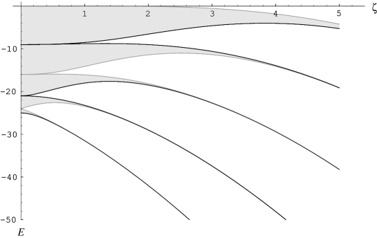
Figure 2: Allowed energy bands (in gray) for the potential (3.1) with $M=5$ as a function of $\zeta$. The solid boundary lines correspond to the algebraically computable (periodic) energies, while the gray boundary lines have been obtained numerically.

The differential equation (3.27) with the potential (3.1) is well-known in the theory of periodic differential equations under the name of Whittaker–Hill’s equation, or Hill’s three-term equation, [26, 27]. It is of interest in the latter context mainly because, unlike the much better known Mathieu’s equation, for certain values of the spectral parameter $E$ it admits so called finite solutions, i.e., solutions of the form

$$\psi(x)=e^{-\frac{\zeta}{2}\cos 2x}\varphi(x)\,,$$

where $\varphi(x)$ is a trigonometric polynomial. It follows from Eq. (3.30) that the algebraic eigenfunctions obtained in this section are finite solutions. In fact, the converse also holds, namely all finite solutions are algebraic eigenfunctions. This follows at once from Theorem 7.9 of Ref. [27], which states (in our notation) that for each $M\in{\mathbb{N}}$ the Whittaker–Hill equation has at most $[M/2]$ gaps of periodic (if $M$ is odd) or anti-periodic (if $M$ is even) type. For even $M$, we have shown that there are exactly $M$ anti-periodic algebraic eigenfunctions, whose corresponding $M$ eigenvalues define exactly $M/2$ gaps of anti-periodic type. Since, for these values of $M$, there are also exactly $M$ anti-periodic finite solutions and eigenvalues, [26], it follows from the Theorem quoted above that the finite solutions coincide (up to a constant factor) with the algebraic eigenfunctions. A similar argument is valid when $M$ is odd.

In order to compare our findings with the classical theory, it is more convenient to use the representation (3.5)–(3.6). Applying the anti-isospectral transformation to Eqs. (2.7) and (2.11) of Section 2, it follows that the algebraic (unnormalized) eigenfunctions can be classified as follows:

$$M$$ even:

$$\psi(x) =e^{-\frac{\zeta}{2}\cos 2x}\,\sum_{k=0}^{\frac{M}{2}-1}\frac{\hat{P}_{k}^{0+}(-E)}{(2k+1)!}\,\cos^{2k+1}x\,,$$ (3.33)

$$\psi(x) =e^{-\frac{\zeta}{2}\cos 2x}\,\sin x\,\sum_{k=0}^{\frac{M}{2}-1}\frac{\hat{P}_{k}^{0-}(-E)}{(2k)!}\,\cos^{2k}x\,;$$ (3.34)

$$M$$ odd:

$$\psi(x) =e^{-\frac{\zeta}{2}\cos 2x}\,\sum_{k=0}^{\frac{M-1}{2}}\frac{\hat{P}_{k}^{+0}(-E)}{(2k)!}\,\cos^{2k}x\,,$$ (3.35)

$$\psi(x) =e^{-\frac{\zeta}{2}\cos 2x}\,\sin x\,\sum_{k=0}^{\frac{M-3}{2}}\frac{\hat{P}_{k}^{-0}(-E)}{(2k+1)!}\,\cos^{2k+1}x\,.$$ (3.36)

In the above formulae, the polynomials $\hat{P}^{\sigma\eta}_{k}$ are defined by the recursion relation (2.12)–(2.13), and $E$ is one of the algebraically computable energies, i.e, $-E$ is a root of the critical polynomials $\hat{P}^{0+}_{M/2}$, $\hat{P}^{0-}_{M/2}$, $\hat{P}^{+0}_{(M+1)/2}$, and $\hat{P}^{-0}_{(M-1)/2}$, respectively. Comparing with the formulae in Section 7.4.1 of Ref. [26] we easily find that, if $\psi(x)$ is an algebraic eigenfunction of one of the four types (3.33)–(3.36), then $e^{\frac{\zeta}{2}\cos 2x}\psi(x)$ is proportional, respectively, to the Ince polynomial $C_{M-1}^{2k+1},\;S_{M-1}^{2k+1},\;C_{M-1}^{2k}$, and $S_{M-1}^{2k}$, where (in the notation of Ince, cf. Ref. [26]) $E=a_{M-1}^{2k+1},\;b_{M-1}^{2k+1},\;a_{M-1}^{2k}$, or $b_{M-1}^{2k}$, respectively.

The results of this section can therefore be interpreted as providing a deep Lie-algebraic justification for the exceptional fact that the Whittaker–Hill equation admits finite solutions. This observation is further corroborated by the fact that other periodic Schrödinger equations known to have finite solutions (in a slightly more general sense) as, for instance, the Lamé equation, are also algebraically QES, [28, 29, 6, 10]. The above results underscore the close connection between the existence of finite solutions of Hill’s equation, on the one hand, and the algebraic QES character of its potential, on the other. This remarkable connection certainly deserves further investigation.

References

- [1] Razavy M 1980 Am. J. Phys. 48 285–8
- [2] Lawrence M C and Robertson G N 1981 Ferroelectrics 34 179–86
- [3] Robertson G N and Lawrence M C 1981 J. Phys. C: Solid State Phys. 14 4559–74
- [4] Matsushita E and Matsubara T 1982 Prog. Theor. Phys. 67 1–19
- [5] Duan X F and Scheiner S 1992 J. Mol. Struct. 270 173–85
- [6] Ulyanov V V and Zaslavskii O B 1992 Phys. Rep. 216 179–251
- [7] Turbiner A V and Ushveridze A G 1987 Phys. Lett. A126 181–3
- [8] Turbiner A V 1988 Commun. Math. Phys. 118 467–74
- [9] González-López A, Kamran N, and Olver P J 1993 Commun. Math. Phys. 153 117–46
- [10] González-López A, Kamran N, and Olver P J 1994 Contemporary Mathematics 160 113–40
- [11] Bender C M and Dunne G V 1996 J. Math. Phys. 37 6–11
- [12] Finkel F, González-López A, and Rodríguez M A 1996 J. Math. Phys. 37 3954–72
- [13] Krajewska A, Ushveridze A, and Walczak Z 1997 Mod. Phys. Lett. A12 1131–44
- [14] Khare A and Mandal B P 1998 Phys. Lett. A239 197–200
- [15] Khare A and Mandal B P 1998 J. Math. Phys. 39 3476–86
- [16] Konwent H, Machnikowski P, Magnuszewski P, and Radosz A 1998 J. Phys. A: Math. Gen. 31 7541–59
- [17] Chihara T S 1978 An Introduction to Orthogonal Polynomials, (New York: Gordon and Breach)
- [18] Shifman M A 1989 Int. J. Mod. Phys. A4 2897–952
- [19] Kofman L, Linde A, and Starobinsky A A 1997 Phys. Rev D 56 3258–95
- [20] Krajewska A, Ushveridze A, and Walczak Z 1997 Mod. Phys. Lett. A12 1225–34
- [21] Turbiner A V 1992 J. Phys. A: Math. Gen. 25 L1087–93
- [22] Finkel F and Kamran N 1998 Adv. Appl. Math. 20 300–22
- [23] Hochstadt H 1986 The Functions of Mathematical Physics (New York: Dover)
- [24] Reed M and Simon B 1978 Analysis of Operators (New York: Academic Press)
- [25] Ince E L 1956 Ordinary Differential Equations (New York: Dover)
- [26] Arscott F M 1964 Periodic Differential Equations (Oxford: Pergamon)
- [27] Magnus W and Winkler S 1979 Hill’s Equation (New York: Dover)
- [28] Alhassid Y, Gürsey F, and Iachello F 1983 Phys. Rev. Lett. 50 873–6
- [29] Turbiner A V 1989 J. Phys. A: Math. Gen. 22 L1–3