TRACE MAPS, INVARIANTS, AND
SOME OF THEIR APPLICATIONS

Trace maps of two-letter substitution rules are investigated with special emphasis on the underlying algebraic structure and on the existence of invariants. We illustrate the results with the generalized Fibonacci chains and show that the well-known Fricke character $I(x,y,z)=x^{2}+y^{2}+z^{2}-2xyz-1$ is not the only type of invariant that can occur. We discuss several physical applications to electronic spectra including the gap-labeling theorem, to kicked two-level systems, and to the classical 1D Ising model with non-commuting transfer matrices.

1 Introduction

Trace maps have been introduced to calculate the spectrum of 1D Kronig-Penney and related models on non-periodic structures like the Fibonacci chain [2, 3]. In the sequel, these maps have found a broad variety of applications, ranging from electronic and phononic structure to 1D scattering and transport (cf. [4, 5, 6, 7] and references therein), from a spin in a magnetic field to kicked two-level systems [8, 9], and from classical to quantum spin systems [10, 11, 12]. Within only a couple of years, the literature on these subjects thus became widespread and hard to survey.

On the other hand, there is a considerable amount of activity on the mathematical aspects of trace maps, ranging from the systematic treatment of substitution rules [13], through computer algebraic investigations [14] to powerful analytic and algebraic results [15, 16, 17, 18, 19, 20], and to the treatment of trace maps as dynamical systems as such [21, 22]. Unfortunately, several if not many of the exact results have not found their way to the explicit treatment of physical systems, partially because they escaped notice and partially because they require some non-trivial mathematics like, e.g., the general gap labeling theorem for Schrödinger operators [17, 23].

It is this gap between the theory of trace maps and their application which we would like to bridge, and we hope that the present article might prove useful for that. It is important to find a systematic, but simple formulation of the trace maps. By this we mean a formulation that is close to that of the Fibonacci case (being the best known) but brings no artificial complications for the generalizations (like singularities induced by coordinate systems). It turns out that the formulation of [13] is very appropriate. Here, all two-letter substitution rules (and we will only consider those) lead to trace maps that are mappings $F$ from $\mbox{\mbox{\hskip 1.00006pt}\rule{0.39993pt}{6.88889pt}\mbox{}{\sf C}}^{3}$ to $\mbox{\mbox{\hskip 1.00006pt}\rule{0.39993pt}{6.88889pt}\mbox{}{\sf C}}^{3}$ where the component mappings are polynomials with integral coefficients only. No poles are present as in alternative formulations with rational functions (cf. [12]), and invariants can be described more easily. Therefore, we will follow this path and occasionally link it to other formulations.

Let us now briefly outline how the remainder of this article is organized. In Sec. 2, we start with some basic definitions and properties of trace maps, using the algebraic approach via the free group of two generators [15, 18]. We then formulate the invariance and transformation properties of the Fricke character $I(x,y,z)=x^{2}+y^{2}+z^{2}-2xyz-1$ [24], a proof of which is given in the Appendix. We illustrate the results with several examples and discuss, in Sec. 3, the generalized Fibonacci chains in some more detail.

Sec. 4 deals with the application to electronic structure, where we apply the gap labeling theorem to the generalized Fibonacci class. For a subclass of models, we also present an intuitive, direct approach which does not rely on the abstract result and, additionally, gives an indexing scheme of the gaps of the approximants. In Sec. 5, we very briefly describe the application to a kicked two-level system which follows a quasiperiodic SU(2) dynamics. Sec. 6 then deals with the classical 1D Ising model with coupling constants and magnetic fields varying according to the non-periodic chain. Here, the trace map gives rise to a direct iteration of the partition function which allows at least an effective numerical treatment of the case of non-commuting transfer matrices. This is followed by the concluding remarks in Sec. 7 and an Appendix where we prove the general transformation law of the Fricke character $I(x,y,z)$ as given in Eq. (2.16).

2 Trace maps and their properties

To explain what a trace map of a two-letter substitution rule is, and what its main properties are in simple but general terms, it is the best to start from the free group generated by two generators $a,b$, i.e., from

$$F_{2}:=<\!<a,b>\!>.$$ (2.1)

Its elements consists of all possible finite words $w=w(a,b,a^{-1},b^{-1})$. $F_{2}$ is an infinite group, multiplication is formal composition of words, and the empty word, $e$, is the neutral element.

A substitution rule $\varrho$ now is a mapping of $F_{2}$ into itself, where - for obvious reasons - we are only interested in homomorphisms, i.e., in $\varrho$’s with the property

$$\varrho(w_{1}w_{2})=\varrho(w_{1})\varrho(w_{2}).$$ (2.2)

Here, the multiplication is the group multiplication in $F_{2}$. To specify a homomorphism, it is therefore sufficient to give the images of the two generators,

$${\varrho}:\begin{array}[]{ccc}a&\rightarrow&w_{a}\\ b&\rightarrow&w_{b}\end{array}$$ (2.3)

where $w_{a}$ and $w_{b}$ are words in $a,b,a^{-1},b^{-1}$, for details we refer to [25, 18]. The concatenation of two homomorphisms, $\varrho_{2}\circ\varrho_{1}$, is well defined. However, one has to insert the rule of $\varrho_{1}$ into that of $\varrho_{2}$ which is a bit against the usual practice. Therefore, we follow [15] and define the multiplication

$$\varrho_{1}\varrho_{2}=\varrho_{1}\cdot\varrho_{2}:=\varrho_{2}\circ\varrho_{1}.$$ (2.4)

With this multiplication, the set of homomorphisms becomes a monoid with the identity as neutral element. We call this monoid $\Theta_{2}=\mbox{Hom}(F_{2})$.

A special role is played by the invertible homomorphisms $\varrho$, i.e., by automorphisms. They form a group $\Phi_{2}$, that is also finitely (but not freely) generated [26, 27, 25]

$$\Phi_{2}:=<\!<U,\sigma,P>\!>$$ (2.5)

where the generators are defined by

$w$	$U(w)$	$\sigma(w)$	$P(w)$
$a$	$ab$	$a^{-1}$	$b$
$b$	$b$	$b$	$a$

For the relations amongst the generators, we refer to p. 164 of [25].

Automorphisms transform the group commutator ${\mbox{\boldmath$K$}}(a,b):=aba^{-1}b^{-1}$ to a conjugate either of itself or of its inverse

$$\varrho({\mbox{\boldmath$K$}}(a,b))={\mbox{\boldmath$K$}}(\varrho(a),\varrho(b))=w\cdot[{\mbox{\boldmath$K$}}(a,b)]^{\pm 1}\cdot w^{-1},$$ (2.6)

where $w$ is an element of $F_{2}$ and $({\mbox{\boldmath$K$}}(a,b))^{-1}={\mbox{\boldmath$K$}}(b,a)$. This can directly be verified by means of the generators, but has also been shown independently [28]. As we will see, this does not extend to $\varrho\not\in\Phi_{2}$.

For the characterization of a substitution rule, it is useful to define the corresponding substitution matrix. First, one maps the elements of $F_{2}$ to lattice points in the square lattice, $\mbox{\sf Z\mbox{}Z}^{2}$, by simply adding the powers of $a$ and the powers of $b$ separately in the word considered. This powercounting induces a homomorphism from $\Phi_{2}=\mbox{Aut}(F_{2})$ to Gl$(2,\mbox{\sf Z\mbox{}Z})=\mbox{Aut}(\mbox{\sf Z\mbox{}Z}^{2})$ [25] and, even more, from the monoid $\Theta_{2}=\mbox{Hom}(F_{2})$ to Hom$(\mbox{\sf Z\mbox{}Z}^{2})=\mbox{Mat}(2,\mbox{\sf Z\mbox{}Z})$, the latter being the monoid of 2x2-matrices with integral elements. Note that Gl$(2,\mbox{\sf Z\mbox{}Z})$ consists of precisely those matrices ${\mbox{\boldmath$R$}}\in\mbox{Hom}(\mbox{\sf Z\mbox{}Z}^{2})$ with det$({\mbox{\boldmath$R$}})=\pm 1$, and it is this determinant which determines the exponent in Eq. (2.6).

We call ${\mbox{\boldmath$R$}}_{\varrho}$ the substitution matrix of the substitution rule $\varrho$, if we can read the number of $a$’s and $b$’s in the words $w_{a}$ and $w_{b}$ rowwise, i.e.,

$${\mbox{\boldmath$R$}}_{\varrho}=\left(\begin{array}[]{ll}\#_{a}(w_{a})&\#_{b}(w_{a})\\ \#_{a}(w_{b})&\#_{b}(w_{b})\\ \end{array}\right)$$ (2.7)

Note that often the transpose of ${\mbox{\boldmath$R$}}_{\varrho}$ is used. With our definition of the product $\varrho\sigma$, see Eq. (2.4), we have indeed

$${\mbox{\boldmath$R$}}_{\varrho\sigma}={\mbox{\boldmath$R$}}_{\varrho}\cdot{\mbox{\boldmath$R$}}_{\sigma},$$ (2.8)

and, e.g., the Fibonacci rule reads $a\rightarrow b,\hskip 2.84526ptb\rightarrow ba\hskip 2.84526pt$ and leads to the matrix

$${\mbox{\boldmath$R$}}_{\varrho}=\left(\begin{array}[]{ll}0&1\\ 1&1\\ \end{array}\right).$$ (2.9)

Of course, different substitution rules can result in the same substitution matrix and the kernel of the homomorphism from $\Theta_{2}$ to Mat$(2,\mbox{\sf Z\mbox{}Z})$ contains all inner automorphisms of $\Phi_{2}$: if $\varrho$ acts as $\varrho(a)=waw^{-1}$ and $\varrho(b)=wbw^{-1}$, one has ${\mbox{\boldmath$R$}}_{\varrho}=\mbox{{\sf 1}\mbox{}\rule{0.39993pt}{6.6736pt}\mbox{\hskip 1.00006pt}}$. The kernel of the mapping from $\Phi_{2}$ to Gl$(2,\mbox{\sf Z\mbox{}Z})$ consists of precisely these inner automorphisms [26] while there are further elements in the general case.

So far, we have only set up the algebraic background. To come to the trace maps, we have to interpret the substitution in the free group as a substitution — and thus a recursion — in the group Sl$(2,\mbox{\mbox{\hskip 1.00006pt}\rule{0.39993pt}{6.88889pt}\mbox{}{\sf C}})$ of 2x2 complex unimodular matrices. We simply insert two matrices ${\mbox{\boldmath$A$}},{\mbox{\boldmath$B$}}$ for the letters $a,b$ and continue. But Sl$(2,\mbox{\mbox{\hskip 1.00006pt}\rule{0.39993pt}{6.88889pt}\mbox{}{\sf C}})$ matrices have very special properties as a consequence of the Cayley-Hamilton theorem of linear algebra, namely

$$\begin{array}[]{rcl}{\mbox{\boldmath$A$}}^{2}&=&\mbox{tr}({\mbox{\boldmath$A$}}){\mbox{\boldmath$A$}}-\mbox{{\sf 1}\mbox{}\rule{0.39993pt}{6.6736pt}\mbox{\hskip 1.00006pt}}\\ {\mbox{\boldmath$A$}}+{\mbox{\boldmath$A$}}^{-1}&=&\mbox{tr}({\mbox{\boldmath$A$}})\mbox{{\sf 1}\mbox{}\rule{0.39993pt}{6.6736pt}\mbox{\hskip 1.00006pt}}\\ {\mbox{\boldmath$A$}}^{n}&=&U_{n-1}(x){\mbox{\boldmath$A$}}-U_{n-2}(x)\mbox{{\sf 1}\mbox{}\rule{0.39993pt}{6.6736pt}\mbox{\hskip 1.00006pt}}\end{array}$$ (2.10)

where $x=\frac{1}{2}\mbox{tr}({\mbox{\boldmath$A$}})$ and $U_{n}(x)$ are Chebyshev’s polynomial of the second kind [29] defined by:

$$\begin{array}[]{ccl}U_{-1}(x)&\equiv&0,\hskip 14.22636ptU_{0}(x)\equiv 1\\ U_{n+1}(x)&=&2xU_{n}(x)-U_{n-1}(x)\;.\\ \end{array}$$ (2.11)

For later use, we run the recursion also backwards and formally obtain polynomials $U_{n}$ for all $n\in\mbox{\sf Z\mbox{}Z}$. Also, Eq. (2.10) is then valid for all integers $n$.

We now define

$$x=\frac{1}{2}\mbox{tr}({\mbox{\boldmath$A$}}),\hskip 14.22636pty=\frac{1}{2}\mbox{tr}({\mbox{\boldmath$B$}}),\hskip 14.22636ptz=\frac{1}{2}\mbox{tr}({\mbox{\boldmath$A$}}{\mbox{\boldmath$B$}}).$$ (2.12)

Then, as a result of Eq. (2.10) and of the general identities $\mbox{tr}({\mbox{\boldmath$A$}}+{\mbox{\boldmath$B$}})=\mbox{tr}({\mbox{\boldmath$A$}})+\mbox{tr}({\mbox{\boldmath$B$}})$ and $\mbox{tr}({\mbox{\boldmath$A$}}{\mbox{\boldmath$B$}})=\mbox{tr}({\mbox{\boldmath$B$}}{\mbox{\boldmath$A$}})$, we find that the traces after one iteration of an arbitrary substitution rule $\varrho$ can be expressed by $x,y,z$ again [13]. This is the corresponding trace map

$$F_{\varrho}:\hskip 5.69054pt\left(\begin{array}[]{c}x\\ y\\ z\end{array}\right)\hskip 5.69054pt\rightarrow\hskip 5.69054pt\left(\begin{array}[]{c}f_{\varrho}(x,y,z)\\ g_{\varrho}(x,y,z)\\ h_{\varrho}(x,y,z)\\ \end{array}\right)$$ (2.13)

where $f_{\varrho},g_{\varrho},h_{\varrho}\in\mbox{\sf Z\mbox{}Z}[x,y,z]$ are three polynomials with integral coefficients. All trace maps defined that way are thus $C^{\infty}$ mappings of $\mbox{\mbox{\hskip 1.00006pt}\rule{0.39993pt}{6.88889pt}\mbox{}{\sf C}}^{3}$ into itself - and interesting dynamical systems as such. Furthermore we find

$$F_{\varrho\sigma}=F_{\varrho}\circ F_{\sigma},$$ (2.14)

compare also [15]. The mapping from the substitution rules to the trace maps is a homomorphism between monoids. For the mapping from $\Phi_{2}$ to Diff($\mbox{\mbox{\hskip 1.00006pt}\rule{0.39993pt}{6.88889pt}\mbox{}{\sf C}}^{3}$), the kernel is known, compare [22]. The mapping induces also a homomorphism from Gl(2,ZZ) to the trace maps, the kernel of which is $\{\pm\mbox{{\sf 1}\mbox{}\rule{0.39993pt}{6.6736pt}\mbox{\hskip 1.00006pt}}\}$.

One of the most celebrated properties of trace maps is the invariance of the polynomial

$$I(x,y,z)=x^{2}+y^{2}+z^{2}-2xyz-1$$ (2.15)

under all trace maps that stem from an automorphism [2, 14, 15, 18]. In our formulation, it follows either immediately from the Nielsen theorem (Eq. (2.6)) (observing that ${\mbox{\boldmath$A$}}\in\mbox{Sl}(2,\mbox{\mbox{\hskip 1.00006pt}\rule{0.39993pt}{6.88889pt}\mbox{}{\sf C}})$ implies $\mbox{tr}({\mbox{\boldmath$A$}})=\mbox{tr}({\mbox{\boldmath$A$}}^{-1})$) or, alternatively, from the generators $U,\sigma,P$ in Eq. (2.3) and their trace maps by simple substitution into Eq. (2.15):

$\varrho$	${\mbox{\boldmath$R$}}_{\varrho}$	$\hskip 48.36967ptF_{\varrho}$
$U$	$\left(\begin{array}[]{cc}1&1\\ 0&1\\ \end{array}\right)$	$\left(\begin{array}[]{c}x\\ y\\ z\\ \end{array}\right)\hskip 5.69054pt\rightarrow\hskip 5.69054pt\left(\begin{array}[]{c}z\\ y\\ 2yz-x\\ \end{array}\right)$
$\sigma$	$\left(\begin{array}[]{cc}-1&0\\ 0&1\\ \end{array}\right)$	$\left(\begin{array}[]{c}x\\ y\\ z\\ \end{array}\right)\hskip 5.69054pt\rightarrow\hskip 5.69054pt\left(\begin{array}[]{c}x\\ y\\ 2xy-z\\ \end{array}\right)$
$P$	$\left(\begin{array}[]{cc}0&1\\ 1&0\\ \end{array}\right)$	$\left(\begin{array}[]{c}x\\ y\\ z\\ \end{array}\right)\hskip 5.69054pt\rightarrow\hskip 22.76219pt\left(\begin{array}[]{c}y\\ x\\ z\\ \end{array}\right)$

This remarkable property appeared in the Fibonacci case in [2], but the theory of Fricke characters, where $I(x,y,z)$ belongs to, is much older (cf. [18] and references therein): It goes back to the last century [24].

But this is not the end of the story because one can show that the Fricke character follows a specific transformation law under any substitution rule, not just under automorphisms. Indeed, for $\varrho\in\mbox{Hom}(F_{2})$, one finds

$$I(F_{\varrho}(x,y,z))=P_{\varrho}(x,y,z)\cdot I(x,y,z)$$ (2.16)

where $P_{\varrho}(x,y,z)\in\mbox{\sf Z\mbox{}Z}[x,y,z]$ is a polynomial with integral coefficients, called the transformation polynomial of $\varrho$. This relation was conjectured on the base of computer algebraic manipulations [14] and proved shortly after [15]. In the Appendix, we give an independent and slightly more complete proof of it.

This relation, together with the general properties mentioned above, has a number of strong consequences. The reader is invited to find some himself. We list the following:

• The variety ${\cal M}_{0}=\{(x,y,z)\in\mbox{\mbox{\hskip 1.00006pt}\rule{0.39993pt}{6.88889pt}\mbox{}{\sf C}}^{3}\mbox{\hskip 5.69054pt}|\mbox{\hskip 5.69054pt}I(x,y,z)=0\}$ is an invariant surface for all trace maps.

• $(1,1,1)$ is a fixed point and $\{(1,-1,-1),(-1,1,-1),(-1,-1,1)\}$ is an invariant set of all trace maps.

• If $(0,0,0)$ is not a fixed point of $F_{\varrho}$, its image lies on ${\cal M}_{0}$.

• If $\varrho\in\Phi_{2}$, $(0,0,0)$ is a fixed point of $F_{\varrho}$. Conversely, $F_{\varrho}(0,0,0)=(0,0,0)$ implies $P_{\varrho}(0,0,0)=1$ and $\nabla P_{\varrho}(0,0,0)=(0,0,0)$, but not $P_{\varrho}\equiv 1$.

• $P_{\varrho}(0,0,0)$ is either $0$ or $1$.

• If $P_{\varrho}$ is constant, we have either $P_{\varrho}\equiv 1$ or $P_{\varrho}\equiv 0$.

• If $\varrho$ is of finite order, $\varrho\in\Phi_{2}$ and $P_{\varrho}\equiv 1$. Furthermore, one has $\varrho^{n}=e$ with $n=1,2,3,4$, or $6$ and $F_{\varrho}^{m}=\mbox{Id}$ with $m=1,2$, or $3$.

• The substitution $\varrho$ is invertible if and only if $P_{\varrho}\equiv 1$.

• The substitution $\varrho$ has nontrivial kernel if and only if $P_{\varrho}\equiv 0$.

• The substitution $\varrho$ is injective but not onto if and only if $P_{\varrho}\not\equiv$ const.

• The set $\{F_{\varrho}\;|\;\varrho\!\in\!\Phi_{2}\}$ of invertible trace maps is a group isomorphic to PGl(2,ZZ).

We cannot give the proofs here, many of which can be found in the work of Peyrière and coworkers, compare [30] and references therein. Let us only remark that one takes profit from using trace orbits of SU(2) matrices and some standard arguments from calculus.

Instead, we would like to remark that, for all trace maps, the dynamics is completely integrable on ${\cal M}_{0}$. Any triple $(x,y,z)$ can be obtained as traces of diagonal matrices, cf. Appendix. Those in turn can be written as diag$(\exp{(i\alpha)},\exp{(-i\alpha)})$, $\alpha\in\mbox{\mbox{\hskip 1.00006pt}\rule{0.39993pt}{6.88889pt}\mbox{}{\sf C}}$, wherefore the multiplication is easily done by counting the exponents of the matrices involved. For any approximant, this can be expressed by the eigenvalues of the substitution matrix ${\mbox{\boldmath$R$}}_{\varrho}$ and is a straightforward generalization of the corresponding property of the Fibonacci chain. This way, one sets up an interesting relation to the theory of pseudo Anosov maps, see [22, 31] for details.

3 The generalized Fibonacci chains and new invariants

In this chapter, we will illustrate some of the properties in the class of generalized Fibonacci chains. The latter are defined by the substitution rules

$$\varrho^{(k,\ell)}:\hskip 5.69054pt\left(\begin{array}[]{l}a\rightarrow b\\ b\rightarrow b^{\ell}a^{k}\end{array}\right),\hskip 14.22636pt{\mbox{\boldmath$R$}}_{\varrho}^{(k,\ell)}=\left(\begin{array}[]{cc}0&1\\ k&\ell\end{array}\right)$$ (3.1)

where $k,\ell\in\mbox{\sf Z\mbox{}Z}$. If the context is clear, we will frequently drop the index $(k,\ell)$. ${\mbox{\boldmath$R$}}_{\varrho}$ is unimodular if and only if $k=\pm 1$. This coincides with $\varrho$ being an automorphism, i.e., invertible. From det$({\mbox{\boldmath$R$}}_{\varrho})=-k$ we also see that $k\not=0$ gives non-singular cases.

What are the corresponding trace maps? A one-page calculation results in

$$F_{\varrho}:\hskip 5.69054pt\left(\begin{array}[]{c}x\\ y\\ z\end{array}\right)\hskip 5.69054pt\rightarrow\hskip 5.69054pt\left(\begin{array}[]{c}y\\ g(x,y,z)\\ h(x,y,z)\\ \end{array}\right)$$ (3.2)

with $g(x,y,z)=U_{k-1}(x)U_{\ell-1}(y)\cdot z-U_{k-1}(x)U_{\ell-2}(y)\cdot x-U_{k-2}(x)U_{\ell-1}(y)\cdot y+U_{k-2}(x)U_{\ell-2}(y)$ and $h(x,y,z)=g(x,y,z)|_{\ell\rightarrow\ell+1}$.

This is equivalent to the formulation of [12]. There, the iteration is given as a difference equation of the form $y_{n+1}=r(y_{n},y_{n-1},y_{n-2})$ with rational function $r$. The latter has singularities as a pure consequence of the coordinates chosen. Therefore, Eq. (3.2) is advantageous. Another page of calculation establishes the transformation polynomial to be

$$P_{\varrho}(x,y,z)=(U_{k-1}(x))^{2}.$$ (3.3)

The cases $k=1$ and $k=-1$ yield $P_{\varrho}\equiv 1$ (and hence the invariance of $I(x,y,z)$) which we know already from the invertibility of $\varrho$ in these cases (independently of $\ell$). The substitution rule $\varrho$ has nontrivial kernel for $k=0$ (e.g., the kernel contains $a^{-\ell}b$) wherefore $P_{\varrho}\equiv 0$ is the necessary consequence. The remaining cases ($k\not\in\{-1,0,1\},\ell\in\mbox{\sf Z\mbox{}Z}$) belong to the class of injective, but non-invertible substitutions. Many properties of Sec. 2 can therefore be demonstrated within this class of examples.

One interesting question is the existence of further invariants. That this indeed is possible can be seen from the case $\ell=1,k=2$ where we find

$$F_{\varrho}:\hskip 5.69054pt\left(\begin{array}[]{c}x\\ y\\ z\end{array}\right)\hskip 5.69054pt\rightarrow\hskip 5.69054pt\left(\begin{array}[]{c}y\\ 2xz-y\\ 4xyz-2x^{2}-2y^{2}+1\\ \end{array}\right).$$ (3.4)

As can be checked directly, this leaves the polynomial $H$ invariant,

$$H(x,y,z)=(4x^{2}-1)y-2xz$$ (3.5)

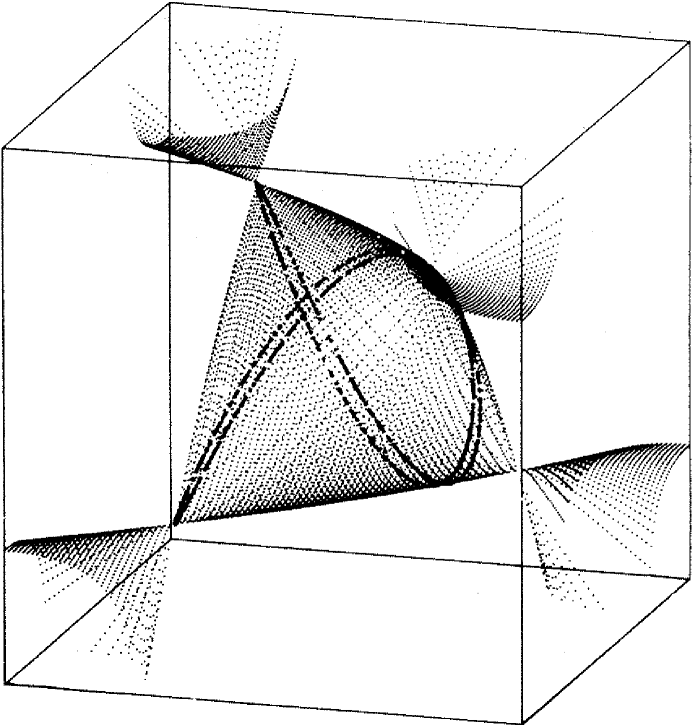
Figure 1: The invariant sheet $S=\{I(x,y,z)=0\}$ and an orbit of the trace map ($k=2,\ell=1$) lying also on the second invariant $H(x,y,z)$ which foliates $S$.

This could be expected from the close relationship of Eq. (3.4) to the period doubling map [32, 14, 33] where an analogous invariant exists. $H$ is different from $I$ and does in fact foliate the single invariant sheet $\{I(x,y,z)=0\}$, see Fig. 1.

A closer look shows that the 1D lines on $\{I=0\}$ are an immediate consequence of ${\mbox{\boldmath$R$}}_{\varrho}$ having an eigenvalue of modulus one. The motion of the dynamical system on $\{I=0\}$ is integrable and related to torus maps. But if there is a direction neither contracted nor expanded, one could expect another invariant of the trace map $F_{\varrho}$ which foliates at least the surface $\{I=0\}$ and, eventually, even the whole $\mbox{\mbox{\hskip 1.00006pt}\rule{0.39993pt}{6.88889pt}\mbox{}{\sf C}}^{3}$.

Now, our substitution matrix ${\mbox{\boldmath$R$}}_{\varrho}$ has eigenvalues $\lambda_{\pm}=\frac{1}{2}(\ell\pm\sqrt{\ell^{2}+4k})$. If they are rational numbers, they are automatically integers. This happens if and only if

$$k=m\cdot\ell+m^{2}$$ (3.6)

with $m$ integer, where we find $\lambda_{+}=\ell+m$ and $\lambda_{-}=-m$. Eq. (3.4) corresponds to $m=1$, and it turns out that it is not a singular case. Indeed, for $k=\ell+1$ in Eq. (3.2), we find the amazingly simple invariant

$$H(x,y,z)=U_{\ell+1}(x)\cdot y-U_{\ell}(x)\cdot z.$$ (3.7)

This is a generalization of Eq. (3.5), for a proof one needs the identities $U_{\ell}^{2}-U_{\ell-1}U_{\ell+1}\equiv 1$ and $U_{\ell}U_{\ell-1}-U_{\ell+1}U_{\ell-2}\equiv U_{1}$. Also for the case $m=-(\ell+1)$, Eq. (3.7) gives the right answer, only $\lambda_{+}$ and $\lambda_{-}$ are interchanged.

The remaining cases are $m=-1$ and $m=1-\ell$. Both result in $k=1-\ell$ and are equivalent. From the extension of the recursion, Eq. (3.2), to negative indices, we know that $U_{-(n+2)}=-U_{n}$ for $n\in\mbox{\sf Z\mbox{}Z}$. By means of the identity $U_{l-1}^{2}-U_{l}U_{l-2}\equiv 1$ one can show the invariance of the polynomial

$$\tilde{H}(x,y,z)=U_{\ell-1}(x)\cdot y-U_{\ell-2}(x)\cdot z=-(U_{-\ell-1}(x)\cdot y-U_{-\ell}(x)\cdot z).$$ (3.8)

This again is a very simple expression and resembles that of Eq. (3.7). We think that no further invariants exist in the class of models investigated here but could not finally settle this question. We can combine the two examples shown formulating $k=1\pm\ell$ and $H^{(\pm)}(x,y,z)=\pm(U_{\pm(\ell+1)}(x)\cdot y-U_{\pm\ell}(x)\cdot z)$. This covers all cases in the class of generalized Fibonacci chains where the corresponding torus map has a unimodular eigenvalue.

Let us close this section with a short remark why invariants are important. The mappings are three dimensional and could show the dynamics of 3D discrete dynamical systems. If an invariant exists, they locally look like 2D systems and inherit the well understood properties of them like period doubling routes to chaos etc., compare the Appendix of [22].

Now, the Fricke character is an invariant precisely for the trace maps of automorphisms, but many interesting trace maps do not stem from automorphisms. Nevertheless, period doubling can occur (as in the so-called period doubling map). The existence of invariants like $H$ or $\tilde{H}$ can explain why — and a further investigation is in progress.

4 Electronic spectra and gap labeling

Amongst the applications of trace maps to physical systems, that to electronic spectra is perhaps the most widespread one [2, 34]. The transfer matrices attached to the different intervals describe the propagation of the amplitudes of the wave function through the chain. In the case of the continuous Schrödinger equation, the transfer matrices for plane waves belong to SU(1,1) [6, 35, 36]. The corresponding trace map acts in $\mbox{\mbox{\hskip 1.00006pt}\rule{0.39993pt}{6.88889pt}\mbox{}{\sf R}}^{3}$ and allows the description of the spectrum, while the underlying matrix system can be used to identify the states. The best way to proceed is to tackle the full Schrödinger equation

$$(-\frac{\hbar^{2}}{2m}\Delta+V(x))\Psi(x)=E\Psi(x)$$ (4.1)

where $V(x)$ is the potential on the chain. But things are a little bit complicated because several quantities become energy dependent. Especially the very invariant $I(x,y,z)$ shows a significant dependence on the energy of the incident wave. Therefore, most authors restrict themselves to the tight-binding case, where Eq. (4.1) is replaced by the discrete version (in suitable units)

$$({\mbox{\boldmath$\cal H$}}\Psi)_{n}=\Psi_{n+1}+\Psi_{n-1}+V_{n}\Psi_{n}=E\Psi_{n},$$ (4.2)

where $I(x,y,z)=\frac{1}{4}(V_{2}-V_{1})^{2}$. $V_{1},V_{2}$ are the potentials on the two different intervals. Although one misses some typical features of the continuous case [6], many generic properties of the spectra remain the same, e.g., in both cases many spectra are Cantor sets with zero Lebesgue measure (see [17] for a criterion). The price one has to pay for going from the full Schrödinger equation to the tight-binding approximation is that in the latter case one needs a whole one parameter set of Hamiltonians which correspond to the single Hamiltonian in the Schrödinger equation [37].

Nevertheless, looking at the gap labeling of the spectra, we can make the restriction to the tight-binding case for simplicity without loss of information. We emphasize that all results can be extended to the continuous equation, compare [37]. For the tight-binding Hamiltonian of Eq. (4.2), the transfer matrices read:

$${\mbox{\boldmath$T$}}_{i}=\left(\begin{array}[]{cr}E-V_{i}&-1\\ 1&0\end{array}\right),$$ (4.3)

and, therefore,

$$\begin{array}[]{cclcl}x&=&\frac{1}{2}\mbox{tr}({\mbox{\boldmath$T$}}_{1})&=&\frac{1}{2}(E-V_{1})\\ &&&&\\ y&=&\frac{1}{2}\mbox{tr}({\mbox{\boldmath$T$}}_{2})&=&\frac{1}{2}(E-V_{2})\\ &&&&\\ z&=&\frac{1}{2}\mbox{tr}({\mbox{\boldmath$T$}}_{2}\cdot{\mbox{\boldmath$T$}}_{1})&=&\frac{1}{2}(E-V_{1})(E-V_{2})-1.\end{array}$$ (4.4)

One could now think of a specific substitution rule $\varrho$ and investigate the spectra by iterative techniques.

Here, we want to follow a slighty different path. First we want to present the famous gap labeling theorem formulated by Bellissard and coworkers. Because it uses non-trivial mathematics we will interpret it in simple words and apply the more concrete version to the well-known case of the generalized Fibonacci sequences. Afterwards, we will give an intuitive way of understanding how the gap labeling theorem works.

Bellissard and coworkers proved the following theorem using techniques of $C^{*}$ algebras and K-Theory [17]:

Let $\cal H$ be a Hamiltonian as in (4.2) with a bounded potential and ${\cal A}_{\mbox{\boldmath$\cal H$}}$ the $C^{*}$ algebra generated by the family of operators obtained from $\cal H$ by translation. The possible values of the Integrated Density of States (IDOS) on the gaps of the spectrum are given by the image of the $K_{0}$ group of the $C^{*}$ algebra ${\cal A}_{\mbox{\boldmath$\cal H$}}$ of the Hamiltonian $\cal H$ under the trace per unit volume, $\tau_{*}(K_{0}({\cal A}_{\mbox{\boldmath$\cal H$}}))$.

This is a general result no matter what the dimension $D$ is. Thinking of the 1D case (4.2) with a potential that takes on only finitely many different values, the gap labeling theorem tells us that the possible values of the IDOS on the gaps are given by all possible frequencies of all possible words in the infinite chain of the substitution $\varrho$. But one can express all these frequencies of words with length greater than one by the frequencies of the words of length one and two. This leads to the ”concrete” gap labeling theorem [17]:

Let $\cal H$ be a Hamiltonian as in (4.2) with the potential given by a primitive substitution, $\varrho$, on a finite alphabet, $A$. The possible values of the IDOS on the gaps in the spectrum are given by the $\mbox{\sf Z\mbox{}Z}(\lambda^{-1})$ module (resp. the part contained in [0,1]), constructed by the components of the normalized eigenvectors $v^{(1)}$ and $v^{(2)}$ to the maximal common eigenvalue $\lambda$ of the substitution matrix for one-letter words ${\mbox{\boldmath$M$}}^{(1)}_{\varrho}$ and for two-letter words ${\mbox{\boldmath$M$}}^{(2)}_{\varrho}$.

The substitution $\varrho$ is called irreducible if, for any pair of letters $a,b$ from the alphabet $A$, the word $\varrho^{k}(a)$ contains $b$ for some $k$. If $k$ can be chosen independently of the letters $a,b$, then $\varrho$ is called primitive. To guarantee the existence of a (half-)infinite word as a fixed point of $\varrho$, one considers a substitution which generates an infinite chain from every letter of the alphabet $A$. There must be at least one letter, $b\in A$ say, so that $\varrho(b)$ begins with $b$, and this letter $b$ must appear in every possible chain.

Let us now apply this theorem. For the calculation of ${\mbox{\boldmath$M$}}^{(1)}_{\varrho}$ and ${\mbox{\boldmath$M$}}^{(2)}_{\varrho}$, we need the substitution of all two-letter words. Let $\varrho(w)=a_{0}a_{1}a_{2}...a_{n}$ be a substitution of a word $w$, then (with the usual notation, cf. [17])

$$\varrho_{N}(w)=(a_{0}a_{1}...a_{N-1})(a_{1}a_{2}...a_{N})...(a_{m-1}a_{m}...a_{m+N-2})$$ (4.5)

is the substitution of an $N$-letter word ($m$ being the total length of $\varrho(a_{0})$ obtained by the powercounting described in Sec. 2). In particular, the two-letter substitution is: $\varrho_{2}(w)=(a_{0}a_{1})(a_{1}a_{2})...(a_{m-1}a_{m})$. Our example is the recursion

$$\begin{array}[]{ccl}a&\rightarrow&b\\ b&\rightarrow&b^{\ell}a^{k}\\ \end{array},$$ (4.6)

which leads to the matrix sytem: ${\mbox{\boldmath$T$}}_{n+1}={\mbox{\boldmath$T$}}_{n-1}^{k}\cdot{\mbox{\boldmath$T$}}_{n}^{\ell}$, compare [6, 12]. The matrix ${\mbox{\boldmath$M$}}_{\varrho}^{(1)}$ is nothing but the transpose of the substitution matrix ${\mbox{\boldmath$R$}}_{\varrho}$, i.e.,

$${\mbox{\boldmath$M$}}_{\varrho}^{(1)}=\left(\begin{array}[]{cc}0&k\\ 1&\ell\end{array}\right),\hskip 14.22636pt\begin{array}[]{l}m_{a}=1\\ m_{b}=k+\ell\end{array}$$ (4.7)

with eigenvalues

$$\lambda_{\pm}=\frac{1}{2}(\ell\pm\sqrt{\ell^{2}+4k}).$$ (4.8)

Let us introduce $D=k(k+\ell-1)$ and exclude the case $D=0$ ($\varrho$ is reducible for $k=0$ and does not increase the length of any word for $k+\ell=1$). Then, we can write the normalized eigenvector to $\lambda_{+}$ as

$$v^{(1)}=\frac{1}{D}\left(\begin{array}[]{ccc}k(k+\ell)&-&k\lambda_{+}\\ -k&+&k\lambda_{+}\end{array}\right).$$ (4.9)

Here, normalization is a statistical one, i.e., $\sum_{i}v_{i}=1$. Also, ${\mbox{\boldmath$M$}}_{\varrho}^{(2)}$ is easy to calculate. We find

$$\begin{array}[]{ccc}aa&\rightarrow&bb\\ ab&\rightarrow&b^{\ell+1}a^{k}\\ ba&\rightarrow&b^{\ell}a^{k}b\\ bb&\rightarrow&b^{\ell}a^{k}b^{\ell}a^{k}\end{array}\hskip 14.22636pt\Rightarrow\hskip 14.22636pt\begin{array}[]{ccl}\varrho(aa)&\rightarrow&(bb)\\ \varrho(ab)&\rightarrow&(bb)\\ \varrho(ba)&\rightarrow&(bb)^{\ell-1}(ba)(aa)^{k-1}(ab)\\ \varrho(bb)&\rightarrow&(bb)^{\ell-1}(ba)(aa)^{k-1}(ab)\end{array}$$ (4.10)

which means

$${\mbox{\boldmath$M$}}_{\varrho}^{(2)}=\left(\begin{array}[]{cccc}0&0&k-1&k-1\\ 0&0&1&1\\ 0&0&1&1\\ 1&1&\ell-1&\ell-1\end{array}\right).$$ (4.11)

The eigenvalues are

$$\lambda\in\{0,0,\frac{1}{2}(\ell\pm\sqrt{\ell^{2}+4k})\}.$$ (4.12)

The (statistically) normalized eigenvector to $\lambda_{+}$ reads

$$v^{(2)}=\frac{1}{D}\left(\begin{array}[]{ccc}(k+\ell)(k-1)&-&(k-1)\lambda_{+}\\ (k+\ell)&-&\lambda_{+}\\ (k+\ell)&-&\lambda_{+}\\ -(2k+\ell)&+&(k+1)\lambda_{+}\end{array}\right),$$ (4.13)

because of $1/\lambda_{+}=(\lambda_{+}-\ell)/k$, and $\lambda_{+}^{2}=k+\ell\lambda_{+}$.

Now the calculation of the frequency module has to be done. This requires some care. First, we observe that the components of $v^{(1)}$ can be obtained by integral linear combinations of components of $v^{(2)}$, and the latter are all of the form $\frac{1}{D}[(m((k+\ell)-\lambda_{+})+n(-(2k+\ell)+(k+1)\lambda_{+})],\hskip 2.84526ptm,n\in\mbox{\sf Z\mbox{}Z}$. This can be rewritten as

$$\frac{1}{D}(\tilde{\mu}+\tilde{\nu}\lambda_{+}),\hskip 14.22636pt\tilde{\mu},\tilde{\nu}\in\mbox{\sf Z\mbox{}Z}$$ (4.14)

but now with the additional constraints

$$\begin{array}[]{ccc}\tilde{\mu}+\tilde{\nu}&\equiv&0\hskip 2.84526pt(D)\\ \tilde{\mu}+(k+\ell)\tilde{\nu}&\equiv&0\hskip 2.84526pt(D)\end{array}.$$ (4.15)

This is necessary to guarantee $m,n\in\mbox{\sf Z\mbox{}Z}$ in the preceeding expression. Remember that $1/\lambda_{+}=(\lambda_{+}-\ell)/k$. It is easy to check that multiplication with $(\lambda_{+}-\ell)$ leads to new numbers $\tilde{\mu}^{\prime},\tilde{\nu}^{\prime}$ which also fulfil Eq. (4.15). Consequently, the $\mbox{\sf Z\mbox{}Z}(\lambda_{+}^{-1})$ module turns out to be

$$\tau_{*}(K_{0}({\cal A}_{\mbox{\boldmath$\cal H$}}))=\{\frac{1}{D}\frac{\tilde{\mu}+\tilde{\nu}\lambda_{+}}{k^{p}}\mbox{\hskip 5.69054pt}|\mbox{\hskip 5.69054pt}\tilde{\mu},\tilde{\nu},p\in\mbox{\sf Z\mbox{}Z},\;\;\begin{array}[]{ccc}\tilde{\mu}+\tilde{\nu}&\equiv&0\hskip 2.84526pt(D)\\ \tilde{\mu}+(k+\ell)\tilde{\nu}&\equiv&0\hskip 2.84526pt(D)\end{array}\}.$$ (4.16)

for the continuous Schrödinger equation and $\tau_{*}(K_{0}({\cal A}_{\mbox{\boldmath$\cal H$}}))\cap[0,1]$ for the tight-binding case.

One has to keep in mind that these are only all possible values the IDOS can take. The gap labeling theorem does not tell us whether all gaps are really open. The most prominent example where gaps are closed systematically is the Thue-Morse sequence [32, 38]. But there, the eigenvalues $\lambda_{\pm}$ are integers, and one has to check whether the frequency module really requires all linear combinations of the components of $v^{(1)}$ and $v^{(2)}$ or not. The analogous question arises for the generalized Fibonacci chains with Eq. (3.6) as condition, but we cannot go into details here.

The special subclass of the metallic Fibonacci sequences $(k=1,\ell\in\mbox{\mbox{\hskip 1.00006pt}\rule{0.39993pt}{6.88889pt}\mbox{}{\sf N}})$ has the module

$$\{\frac{1}{\ell}(\tilde{\mu}+\tilde{\nu}\lambda_{+})\mbox{\hskip 5.69054pt}|\mbox{\hskip 5.69054pt}\tilde{\mu},\tilde{\nu}\in\mbox{\sf Z\mbox{}Z},\hskip 14.22636pt\tilde{\mu}+\tilde{\nu}\equiv 0\hskip 2.84526pt(\ell)\},$$ (4.17)

whereas the largest eigenvalues of the substitution matrices are given by the metallic means:

$$\lambda_{+}=\frac{1}{2}(\ell+\sqrt{\ell^{2}+4})=[\ell;\ell,\ell,\ell,...].$$ (4.18)

Looking at these chains one is able to give a more heuristic but intuitive way of understanding how the gap labeling theorem works.

Let us introduce the generalized Fibonacci numbers, $f_{n}^{(\ell)}$, by

$$f_{n+1}^{(\ell)}=\ell\cdot f_{n}^{(\ell)}+f_{n-1}^{(\ell)},\hskip 14.22636ptf_{0}^{(\ell)}=0,\hskip 8.53581ptf_{1}^{(\ell)}=1.$$ (4.19)

This choice of initial conditions will prove useful shortly. We observe that two consecutive numbers are coprime because the greatest common divisor obeys gcd$(f_{n}^{(\ell)},f_{n+1}^{(\ell)})=\mbox{gcd}(f_{n}^{(\ell)},\ell\cdot f_{n}^{(\ell)}+f_{n-1}^{(\ell)})=\mbox{gcd}(f_{n}^{(\ell)},f_{n-1}^{(\ell)})$, i.e., coprimality is inherited from the initial conditions.

If we now consider the series of periodic approximants starting from $b$, i.e., $b\rightarrow b^{\ell}a\rightarrow(b^{\ell}a)^{\ell}b$ etc., we know that these approximants are optimal in the following sense: a given approximant of length $g_{n}^{(\ell)}$, where

$$g_{n}^{(\ell)}=f_{n}^{(\ell)}+f_{n-1}^{(\ell)},$$ (4.20)

is closer to the limit structure than any given other approximant of length $L\leq g_{n}^{(\ell)}$. One therefore expects that the structure of the IDOS of this approximant is as close to the limit IDOS as possible with approximants up to that length. In particular, the values of the IDOS on the gaps converge rapidly.

It is tempting to select series of IDOS plateaus in the sequence of approximants in such a way that the corresponding gaps belong to each other (by quantum numbers, strength, symmetry, etc.). Then, if one can find a labeling, the limit $n\rightarrow\infty$ should reproduce the result of the general theorem described above. The chains with the metallic means facilitate this procedure. Here, gaps in consecutive approximants can be attached to one another by the following simple rule. Given a gap in the $n$-th approximant. Then, in the step from $n$ to $n+1$, one always grabs the closest IDOS value possible. If this is not unique (which happens only occasionally) one takes both possibilities as two branches. One branch will actually correspond to a new series of gaps, but that is hard to see in general and does not matter for the limit.

Now comes the trick: the gaps in the $n$-th approximant lead to IDOS values of the form

$$\frac{m}{f_{n}^{(\ell)}+f_{n-1}^{(\ell)}},\hskip 14.22636pt0\leq m\leq f_{n}^{(\ell)}+f_{n-1}^{(\ell)},$$ (4.21)

which is an exact result from Bloch theory for the periodic approximants. But, $m$ can be written as

$$m=\mu\cdot f_{n}^{(\ell)}+\nu\cdot f_{n-1}^{(\ell)},\hskip 14.22636pt\mu,\nu\in\mbox{\sf Z\mbox{}Z},$$ (4.22)

because $f_{n}^{(\ell)}$ and $f_{n-1}^{(\ell)}$ are coprime. Taking $(\mu,\nu)$ as label, it turns out that Eq. (4.22) selects series of IDOS plateaus — and hence gaps — that follow the rule mentioned before! Furthermore, it is easy to see that neither possible gaps are missed nor index pairs are missing (as long as $\mu\cdot f_{n}^{(\ell)}+\nu\cdot f_{n-1}^{(\ell)}\in[0,f_{n}^{(\ell)}+f_{n-1}^{(\ell)}]$). It now is straightforward to calculate the limit points which gives the set

$$\{\frac{\lambda_{+}-1}{\ell}(\mu+\nu\frac{1}{\lambda_{+}})\mbox{\hskip 5.69054pt}|\mbox{\hskip 5.69054pt}\mu,\nu\in\mbox{\sf Z\mbox{}Z}\}\cap[0,1].$$ (4.23)

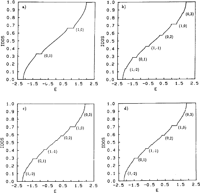
Figure 2: The approximants of the octonacci chain, $k=1,\ell=2$, with length a) 3, b) 7, c) 17, d) 41 and the gap labels, $(\mu,\nu)$, starting with the 3- and the 7-approximant.

A similar argument was recently given for the original Fibonacci chain [39] where this procedure is most simple. A simple substitution shows that Eq. (4.23) precisely reproduces the result obtained above in Eq. (4.17), including the modulo condition. The labels obtained from Eq. (4.23) are slightly handier as can be seen in Fig. 2, where, as an example, we show the IDOS of the first approximants of the ’octonacci’ chain, ($k=1,\ell=2$), and the index pairs $(\mu,\nu)$ starting with the approximants of length 3 and 7.

Let us finally remark that the coincidence of the abstract and the concrete approach has a strong consequence: As far as we calculated, all gaps of the approximants involved here are open (for suitable choices of potentials). But from the second approach, it is meaningful to conjecture that all gaps are open for the class of metallic Fibonacci chains. For a proof, one could try pertubative arguments along the lines of [32] because these chains are quasiperiodic with embedding dimension 2, compare [6]. This will be given elsewhere.

5 Some properties of kicked two-level systems

As already mentioned in the Introduction, matrices and trace maps derived from two-letter substitution rules find applications in a variety of problems. Here, we briefly describe the case of SU(2) dynamics. The latter appears naturally in the solution of Schrödinger’s equation for an electron or another particle with spin $s=1/2$ in a magnetic field $\vec{B}$ [40].

$$i\hbar\dot{\Psi}=\mu_{B}\vec{B}{\vec{\mbox{\boldmath$\sigma$}}}\Psi$$ (5.1)

with Bohr’s magneton $\mu_{B}=\frac{\hbar}{2m_{0}}$, Pauli’s spin matrices ${\mbox{\boldmath$\sigma$}}_{i}$, a spinor $\Psi$ of two components, and

$$\vec{B}{\vec{\mbox{\boldmath$\sigma$}}}=\left(\begin{array}[]{cc}B_{3}&B_{1}-iB_{2}\\ B_{1}+iB_{2}&-B_{3}\end{array}\right).$$ (5.2)

We have written the time-dependent equation in Eq. (5.1) because the stationary case with constant magnetic field is completely integrable [40] and hence less interesting than the truly time-dependent one. Here we are interested in a special class of time-dependent fields that allow the application of the recursive transfer matrix techniques, where transfer is now in time.

Rewriting Eq. (5.1) slightly, we obtain the structural core as

$$\dot{\Psi}=-i{\mbox{\boldmath$\cal H$}}(t)\Psi$$ (5.3)

with hermitian and traceless operator ${\mbox{\boldmath$\cal H$}}(t)$. The (formal) solution is

$$\Psi(t)={\mbox{\boldmath$U$}}(t,t_{0})\Psi(t_{0})$$ (5.4)

with

$${\mbox{\boldmath$U$}}(t,t_{0})=\mbox{T}[\exp{(-i\int_{t_{0}}^{t}{\mbox{\boldmath$\cal H$}}(\tau)d\tau)}].$$ (5.5)

The time evolution operator $U$ is a time-dependent SU(2) matrix, and T denotes time-odering [41].

Let us now think of a time sequence following the generalized Fibonacci chain, cf. (4.6). With ${\mbox{\boldmath$U$}}_{n}:={\mbox{\boldmath$U$}}(t_{n},t_{0})$ we obtain

$${\mbox{\boldmath$U$}}_{n+1}={\mbox{\boldmath$U$}}_{n-1}^{k}\cdot{\mbox{\boldmath$U$}}_{n}^{\ell}$$ (5.6)

for the SU(2) dynamics. The treatment of this matrix system gives full information but goes beyond the scope of the present article. For a summary of what can be done with that we refer to [18]. Here, we follow [11] and consider the trace systems only which gives insight into the behaviour of certain observables. Let us formulate it for the Fibonacci case ($k=\ell=1$), the extension to the other examples is immediate.

To be explicit in the formulas, we will consider $\delta$-kicks on the time intervals, more precisely, at the beginning of them. Any SU(2) matix $A$ can be written in the form

$${\mbox{\boldmath$A$}}=\exp{(-ia{\vec{n}}{\vec{\mbox{\boldmath$\sigma$}}})}=\cos{(a)}\mbox{{\sf 1}\mbox{}\rule{0.39993pt}{6.6736pt}\mbox{\hskip 1.00006pt}}-i\sin{(a)}{\vec{n}}{\vec{\mbox{\boldmath$\sigma$}}}$$ (5.7)

with $a\in\mbox{\mbox{\hskip 1.00006pt}\rule{0.39993pt}{6.88889pt}\mbox{}{\sf R}}^{+}$ and ${\vec{n}}$ a unit vector (hence, $({\vec{n}}{\vec{\mbox{\boldmath$\sigma$}}})^{2}=\mbox{{\sf 1}\mbox{}\rule{0.39993pt}{6.6736pt}\mbox{\hskip 1.00006pt}}$). From the relation

$$[{\vec{n}}{\vec{\mbox{\boldmath$\sigma$}}},{\vec{n}}^{\prime}{\vec{\mbox{\boldmath$\sigma$}}}]=2i\epsilon_{k\ell m}n_{k}n_{\ell}^{\prime}{\mbox{\boldmath$\sigma$}}_{m}$$ (5.8)

we can conclude that transfer matrices of the elementary intervals certainly commute if the kicks are in the same direction. But then, the real traces run on $\{I=0\}$ and stay bounded, $|x|\leq 1,|y|\leq 1,|z|\leq 1$. The orbit belongs to the pseudo Anosov system, compare [31, 22]. The question now is what happens off this surface.

Consider the kicks $\delta(t)a_{j}{\vec{n}}_{j}{\vec{\mbox{\boldmath$\sigma$}}},\hskip 2.84526ptj=0,1$ for the two elementary time intervals. We find

$${\mbox{\boldmath$U$}}^{(j)}=\exp{(-i\int_{0}^{t_{j}}\delta(t)a_{j}{\vec{n}}_{j}{\vec{\mbox{\boldmath$\sigma$}}}dt)}=\cos{(a_{j})}\mbox{{\sf 1}\mbox{}\rule{0.39993pt}{6.6736pt}\mbox{\hskip 1.00006pt}}-i\sin{(a_{j})}{\vec{n}}_{j}{\vec{\mbox{\boldmath$\sigma$}}}$$ (5.9)

with

$$({\vec{n}}_{0}{\vec{\mbox{\boldmath$\sigma$}}})\cdot({\vec{n}}_{1}{\vec{\mbox{\boldmath$\sigma$}}})=({\vec{n}}_{0}{\vec{n}}_{1})\mbox{{\sf 1}\mbox{}\rule{0.39993pt}{6.6736pt}\mbox{\hskip 1.00006pt}}+i({\vec{n}}_{0}\times{\vec{n}}_{1}){\vec{\mbox{\boldmath$\sigma$}}}.$$ (5.10)

We can work out the product ${\mbox{\boldmath$U$}}^{(2)}={\mbox{\boldmath$U$}}^{(0)}{\mbox{\boldmath$U$}}^{(1)}$ and obtain

$${\mbox{\boldmath$U$}}^{(2)} = \{\cos{(a_{0})}\cos{(a_{1})}-\sin{(a_{0})}\sin{(a_{1})}{\vec{n}}_{0}{\vec{n}}_{1}\}\mbox{{\sf 1}\mbox{}\rule{0.39993pt}{6.6736pt}\mbox{\hskip 1.00006pt}}$$

$$+i\{{\vec{n}}_{0}\times{\vec{n}}_{1}\sin{(a_{0})}\sin{(a_{1})}-{\vec{n}}_{0}\sin{(a_{0})}\cos{(a_{1})}-{\vec{n}}_{1}\cos{(a_{0})}\sin{(a_{1})}\}{\vec{\mbox{\boldmath$\sigma$}}}$$

This gives the initial conditions for the traces as

$$\begin{array}[]{l}x_{0}=\cos{(a_{0})},\hskip 11.38109ptx_{1}=\cos{(a_{1})},\\ x_{2}=\cos{(a_{0})}\cos{(a_{1})}-\sin{(a_{0})}\sin{(a_{1})}({\vec{n}}_{0}{\vec{n}}_{1}).\end{array}$$ (5.12)

With some further calculations one can establish the formula

$$I(x_{0},x_{1},x_{2})=[({\vec{n}}_{0}{\vec{n}}_{1})^{2}-1]\cdot(\sin{(a_{0})}\sin{(a_{1})})^{2}$$ (5.13)

which shows $-1\leq I\leq 0$, as it must be for SU(2).

One can now start from $I=-1$ and go to $I=0$ by an adiabatic change of parameters. This way, one could try to follow (for the Fibonacci case, say,) the period doubling route to chaos, described recently in [22]. It is an interesting question whether one could experimentally find the conservative feigenvalues predicted theoretically.

6 Classical 1D Ising model with non-commuting transfer matrices

Let us consider a linear chain of $N$ Ising spins $\sigma_{j}\in\{\pm 1\}$, $j=1,\ldots,N$, with the energy of a configuration $\sigma=(\sigma_{1},\sigma_{2},\ldots,\sigma_{N})$ being given by [42]

$$E(\sigma)\;\;=\;\;-\sum_{j=1}^{N}\left(J_{j,j+1}\sigma_{j}\sigma_{j+1}\>+\>H_{j}\sigma_{j}\right),$$ (6.1)

where we choose periodic boundary conditions, i.e., $\sigma_{N+1}=\sigma_{1}$. The canonical partition function $Z^{(N)}$ of this system is obtained as a sum over all possible configurations $\sigma$ as follows

$$Z^{(N)}\;\;=\;\;\sum_{\sigma}\prod_{j=1}^{N}\exp\left(K_{j,j+1}\sigma_{j}\sigma_{j+1}+h_{j}\sigma_{j}\right)$$ (6.2)

with $K_{j,j+1}=J_{j,j+1}/k_{B}T$ and $h_{j}=H_{j}/k_{B}T$. Here, $T$ is the temperature and $k_{B}$ denotes Boltzmann’s constant. The corresponding free energy per site $F^{(N)}$ is given by $F^{(N)}=-\frac{1}{N}\log Z^{(N)}$ where we absorbed the factor $1/(k_{B}T)$ into the definition in order to obtain a dimensionless quantity.

Eq. (6.2) can be rewritten in the following way (see [42])

$$Z^{(N)} = \sum_{\sigma}\;{\mbox{\boldmath$\cal T$}}^{(1,2)}(\sigma_{1},\sigma_{2})\>{\mbox{\boldmath$\cal T$}}^{(2,3)}(\sigma_{2},\sigma_{3})\>\cdots{\mbox{\boldmath$\cal T$}}^{(N,1)}(\sigma_{N},\sigma_{1})$$

$$= \mbox{tr}\left({\mbox{\boldmath$\cal T$}}^{(1,2)}{\mbox{\boldmath$\cal T$}}^{(2,3)}\cdots{\mbox{\boldmath$\cal T$}}^{(N,1)}\right)$$

$$= \mbox{tr}\left({\mbox{\boldmath$\cal T$}}^{(N)}\right)$$

where the elementary transfer matrix ${\mbox{\boldmath$\cal T$}}^{(j,j+1)}$ is given by the $2\!\times\!2$ matrix [42]

$${\mbox{\boldmath$\cal T$}}^{(j,j+1)}\;\;=\;\;\left(\begin{array}[]{ll}\exp\left(K_{j,j+1}+\frac{h_{j}+h_{j+1}}{2}\right)&\exp\left(-K_{j,j+1}\right)\\ \exp\left(-K_{j,j+1}\right)&\exp\left(K_{j,j+1}-\frac{h_{j}+h_{j+1}}{2}\right)\end{array}\right)\;\;,$$ (6.4)

while ${\mbox{\boldmath$\cal T$}}^{(N)}$ denotes the transfer matrix of $N$ sites. Note that the transfer matrices at different sites in general do not commute and therefore cannot be diagonalized simultaneously.

So far we have not specified the coupling constants $K_{j,j+1}$ and the magnetic fields $h_{j}$. A particularly interesting case is that of coupling constants $K_{j,j+1}=1$ and quasiperiodic fields $h_{j}$. The ground state properties have recently been analyzed exactly [43]. Here, we now want to consider non-periodic chains where $K_{j,j+1}$ and $h_{j}$ are modulated according to the two-letter substitution rule $\varrho^{(k,\ell)}$ (3.1) but taking only two possible values. To be more precise, consider a particular word $w_{n}$ ($w_{0}=a$, $w_{1}=b$, $w_{n+1}=\varrho^{(k,\ell)}(w_{n})$) with length $N_{n}=f^{(k,\ell)}_{n}+kf^{(k,\ell)}_{n-1}$, where the $f^{(k,\ell)}_{n}$ are defined (generalizing Eq. (4.19)) by

$$f^{(k,\ell)}_{n+1}\;\;=\;\;\ell f^{(k,\ell)}_{n}\>+\>kf^{(k,\ell)}_{n-1}\hskip 28.45274ptf_{0}^{(k,\ell)}=0,\hskip 14.22636ptf_{1}^{(k,\ell)}=1\;.$$ (6.5)

To $w_{n}$ we associate an Ising spin chain with $N_{n}=N_{n}^{(k,\ell)}$ sites in the following way: We choose $K_{j,j+1}=K^{(i)}$ and $h_{j}=h^{(i)}$ ($i=0,1$) where $i=0$ if the $j^{\mbox{th}}$ letter in the word $w_{n}$ is an $a$ and $i=1$ otherwise. Hence the chains we consider are characterized by four real parameters $K^{(i)}$ and $h^{(i)}$, $i=0,1$, and the two numbers $k,\ell\in\mbox{\sf Z\mbox{}Z}$ which determine the substitution rule. Denoting the transfer matrix of the chain associated with the word $w_{n}$ by ${\mbox{\boldmath$\cal T$}}_{n}$, one has the following recursive equation for the transfer matrices

$${\mbox{\boldmath$\cal T$}}_{n+1}\;\;=\;\;{\mbox{\boldmath$\cal T$}}_{n}^{\,\ell}\>{\mbox{\boldmath$\cal T$}}_{n-1}^{\,k}$$ (6.6)

with initial conditions

$${\mbox{\boldmath$\cal T$}}_{i}\;\;=\;\;\left(\begin{array}[]{ll}\exp\left(K^{(i)}+h^{(i)}\right)&\exp\left(-K^{(i)}\right)\\ \exp\left(-K^{(i)}\right)&\exp\left(K^{(i)}-h^{(i)}\right)\end{array}\right)\hskip 28.45274pti=0,1$$ (6.7)

corresponding to the words $w_{0}=a$ and $w_{1}=b$.

Now, we are almost in the position to use the trace map (3.2) to obtain a recursive relation for the partition function and hence for the free energy of our chains. In order to do so, we define unimodular matrices $\tilde{\mbox{\boldmath$\cal T$}}_{n}=\frac{1}{d_{n}}{\mbox{\boldmath$\cal T$}}_{n}$ where $d_{n}=\sqrt{\det{\mbox{\boldmath$\cal T$}}_{n}}$ and use the trace map (3.2) for

$$x_{n}\;\;=\;\;\frac{1}{2}\mbox{tr}\left(\tilde{\mbox{\boldmath$\cal T$}}_{n}\right)\;\;=\;\;\frac{1}{2d_{n}}Z_{n}$$ (6.8)

which yields a recursion relation for the partition function $Z_{n}=\mbox{tr}({\mbox{\boldmath$\cal T$}}_{n})$ of the chain associated with the word $w_{n}$, compare [44] for an equivalent formulation with a nested iteration. The determinants are simply given by (see Eq. (6.5))

$$d_{n+1} = d_{n}d_{n-1}$$ (6.9)

$$= (d_{0})^{kf^{(k,\ell)}_{n-1}}(d_{1})^{f^{(k,\ell)}_{n}}$$

with $d_{i}=\sqrt{2\sinh(2K^{(i)})}$, $i=0,1$. In particular, all $d_{n}$ are non-zero if $d_{0}$ and $d_{1}$ are different from zero, i.e. if both coupling constants $K^{(i)}$, $i=0,1$, do not vanish. Thus the trick we used to be able to apply the trace map (3.2) to the transfer matrices of the Ising chain was to split the recursion relation (6.6) for the transfer matrices into two parts: one for the trace of the transfer matrices and a rather trivial one for their determinant.

Explicitly, the trace map (3.2) becomes

$$\left(\begin{array}[]{c}x_{n}\\ y_{n}\\ z_{n}\end{array}\right)\hskip 11.38109pt\longrightarrow\hskip 11.38109pt\left(\begin{array}[]{c}x_{n+1}\\ y_{n+1}\\ z_{n+1}\\ \end{array}\right)\hskip 5.69054pt=\hskip 5.69054pt\left(\begin{array}[]{c}y_{n}\\ g(x_{n},y_{n},z_{n})\\ h(x_{n},y_{n},z_{n})\\ \end{array}\right),$$ (6.10)

compare Eq. (3.2), with starting values

$$x_{0} = \frac{\mbox{tr}\left({\mbox{\boldmath$\cal T$}}_{0}\right)}{2d_{0}}\hskip 11.38109pt=\hskip 11.38109pt\frac{\exp K^{(0)}\cosh h^{(0)}}{\left(2\sinh(2K^{(0)})\right)^{1/2}}$$

$$y_{0} = \frac{\mbox{tr}\left({\mbox{\boldmath$\cal T$}}_{1}\right)}{2d_{1}}\hskip 11.38109pt=\hskip 11.38109pt\frac{\exp K^{(1)}\cosh h^{(1)}}{\left(2\sinh(2K^{(1)})\right)^{1/2}}$$ (6.11)

$$z_{0} = \frac{\mbox{tr}\left({\mbox{\boldmath$\cal T$}}_{0}{\mbox{\boldmath$\cal T$}}_{1}\right)}{2d_{0}d_{1}}$$

$$= \frac{\exp(K^{(0)}+K^{(1)})\cosh(h^{(0)}+h^{(1)})+\exp(-(K^{(0)}+K^{(1)}))}{2\left(\sinh(2K^{(0)})\sinh(2K^{(1)})\right)^{1/2}}.$$

Iterating the trace map thus corresponds to performing the thermodynamic limit $n\rightarrow\infty$.

In this way the trace map (3.2) provides an efficient way to compute the free energy in the infinite size limit numerically. Unfortunately, an analytic solution to the recursion relation is only known for the case that the starting point lies on the invariant variety ${\cal M}_{0}=\{(x,y,z)\in\mbox{\mbox{\hskip 1.00006pt}\rule{0.39993pt}{6.88889pt}\mbox{}{\sf C}}^{3}\mbox{\hskip 5.69054pt}|\mbox{\hskip 5.69054pt}I(x,y,z)=0\}$ which turns out to be equivalent to the requirement that the transfer matrices ${\mbox{\boldmath$\cal T$}}_{0}$ and ${\mbox{\boldmath$\cal T$}}_{1}$ commute. For this case, the solution is trivial since one only counts the relative frequencies of the two different couplings in the chain.

It should be added that recursion relations for the magnetization (one-point function) can be derived by similar means. So far, we have not been able to extend this procedure to higher correlation functions. A renormalization group analysis (see [45]) of the field-free case ($h^{(0)}=h^{(1)}=0$) gives the substitution matrix as linearization at the zero-temperature fixed point and hence the thermal exponent $\alpha=1$ as one would expect. Further work along these directions is in progress.

7 Concluding remarks

Having described structure and applications of trace maps of two-letter substitution rules, we will briefly address further developments. It seems that the mathematical aspects are understood fairly well. Nevertheless, the trace maps as dynamical systems on their own right show interesting features that deserve further exploration: orbit structure, nontrivial symmetries, reversibility, period-doubling, and pseudo Anosov structure, compare [22] for some results.

The physical applications could still profit from simply soaking up known exact results. A prominent example is the gap labeling where the combination of algebraic methods, generalized Bloch theory and pertubation theory improves the understanding of spectra and wave functions. For the latter, the extension to matrix maps should also be studied in more detail. A similar remark holds true of the other applications. Kicked two-level systems and spin systems are not yet brought to the understanding possible.

Another, rather restrictive point is the treatment of two-letter rules: more than that is desirable. Several results are known for $n$-letter substitution rules, compare [17, 9, 30, 46, 47], but the generality of the findings is lacking. Many simple properties do not extend, e.g., trace maps are higher dimensional and investigation of invariants is much more complicated. Only the gap labeling theorem still applies in full generality, wherefore further work in this direction will be needed.

Appendix

If $F_{\varrho}$ is the trace map of a two-letter substitution rule $\varrho\in\mbox{Hom}(F_{2})$, then there is a uniquely defined transformation polynomial $P_{\varrho}\in\mbox{\sf Z\mbox{}Z}[x,y,z]$ such that the Fricke character $I(x,y,z)=x^{2}+y^{2}+z^{2}-2xyz-1$ shows the transformation law

$$I(F_{\varrho}(x,y,z))=P_{\varrho}(x,y,z)\cdot I(x,y,z)$$ (A.1)

Here, the standard basis is used, i.e., $x=\frac{1}{2}\mbox{tr}({\mbox{\boldmath$A$}}),y=\frac{1}{2}\mbox{tr}({\mbox{\boldmath$B$}}),z=\frac{1}{2}\mbox{tr}({\mbox{\boldmath$A$}}{\mbox{\boldmath$B$}})$ with ${\mbox{\boldmath$A$}},{\mbox{\boldmath$B$}}\in\mbox{Sl}(2,\mbox{\mbox{\hskip 1.00006pt}\rule{0.39993pt}{6.88889pt}\mbox{}{\sf C}})$. Instead of the complex numbers, one can also use any other algebraically complete field.

For the proof of this remarkable equation, the variety ${\cal M}_{0}=\{(x,y,z)\in\mbox{\mbox{\hskip 1.00006pt}\rule{0.39993pt}{6.88889pt}\mbox{}{\sf C}}^{3}\mbox{\hskip 5.69054pt}|\mbox{\hskip 5.69054pt}I(x,y,z)=0\}$ plays an important role. We first observe that

$$\mbox{tr}({\mbox{\boldmath$K$}}({\mbox{\boldmath$A$}},{\mbox{\boldmath$B$}})-\mbox{{\sf 1}\mbox{}\rule{0.39993pt}{6.6736pt}\mbox{\hskip 1.00006pt}})=4\cdot I(x,y,z)$$ (A.2)

for unimodular 2x2-matrices, where ${\mbox{\boldmath$K$}}({\mbox{\boldmath$A$}},{\mbox{\boldmath$B$}})={\mbox{\boldmath$A$}}{\mbox{\boldmath$B$}}{\mbox{\boldmath$A$}}^{-1}{\mbox{\boldmath$B$}}^{-1}$ is the group commutator. This follows straightforwardly from the Cayley-Hamilton theorem. We observe next that any triple $(x,y,z)\in{\cal M}_{0}$ can be seen as traces of diagonal matrices since we can simply choose ${\mbox{\boldmath$A$}}=\mbox{diag}(\alpha,\alpha^{-1}),\hskip 5.69054pt{\mbox{\boldmath$B$}}=\mbox{diag}(\beta^{\varepsilon},\beta^{-\varepsilon})$, with $\alpha=x+\sqrt{x^{2}+1},\hskip 5.69054pt\beta=y+\sqrt{y^{2}+1}$, and $\varepsilon=\pm 1$. Then, we find from the condition $I(x,y,z)=0$ (a quadratic equation in $z$), the relation $2z=\alpha\beta^{\varepsilon}+1/(\alpha\beta^{\varepsilon})$, i.e., $z=\frac{1}{2}\mbox{tr}({\mbox{\boldmath$A$}}{\mbox{\boldmath$B$}})$. The two choices of $\varepsilon$ cover the two possible solutions of the quadratic equation.

Observing that $[{\mbox{\boldmath$A$}},{\mbox{\boldmath$B$}}]=0$ implies ${\mbox{\boldmath$K$}}({\mbox{\boldmath$A$}},{\mbox{\boldmath$B$}})=\mbox{{\sf 1}\mbox{}\rule{0.39993pt}{6.6736pt}\mbox{\hskip 1.00006pt}}$, we see from Eq. (A.2) that $I(x,y,z)=0$ implies $I(F_{\varrho}(x,y,z))=0$. On the other hand, we know that

$$P_{\varrho}(x,y,z)=\frac{I(F_{\varrho}(x,y,z))}{I(x,y,z)}=\frac{\mbox{tr}({\mbox{\boldmath$K$}}(\varrho({\mbox{\boldmath$A$}}),\varrho({\mbox{\boldmath$B$}}))-\mbox{{\sf 1}\mbox{}\rule{0.39993pt}{6.6736pt}\mbox{\hskip 1.00006pt}})}{\mbox{tr}({\mbox{\boldmath$K$}}({\mbox{\boldmath$A$}},{\mbox{\boldmath$B$}})-\mbox{{\sf 1}\mbox{}\rule{0.39993pt}{6.6736pt}\mbox{\hskip 1.00006pt}})}.$$ (A.3)

Thus, $P_{\varrho}$ is the quotient of two polynomials with integral coefficients. The denominator, $I(x,y,z)$, is irreducible in $\mbox{\sf Z\mbox{}Z}[x,y,z]$, and the numerator polynomial vanishes at least on the set ${\cal M}_{0}$. From this, we can conclude that the denominator divides the numerator. Since this can been seen in an elementary way, we will briefly give the argument.

Consider a polynomial $Q\in\mbox{\mbox{\hskip 1.00006pt}\rule{0.39993pt}{6.88889pt}\mbox{}{\sf C}}[x,y,z]$ that vanishes at least on ${\cal M}_{0}$. If $Q$ is of less than second order in $x,y$, or $z$, we can only have $Q\equiv 0$. To show this, assume, without loss of generality, $Q$ linear in $z$, i.e., $Q=\xi(x,y)+\eta(x,y)\cdot z$ with polynomials $\xi$ and $\eta$. For arbitrary $x,y\in\mbox{\mbox{\hskip 1.00006pt}\rule{0.39993pt}{6.88889pt}\mbox{}{\sf C}}$ we can find $z_{\pm}=z_{\pm}(x,y)$ so that $(x,y,z_{+})\in{\cal M}_{0}$ and $(x,y,z_{-})\in{\cal M}_{0}$. Consequently, $Q$ must also vanish on these points, which gives

$$z_{+}\cdot\eta(x,y)=z_{-}\cdot\eta(x,y).$$ (A.4)

But we can choose $(x,y)$ such that $z_{+}(x,y)\not=z_{-}(x,y)$ wherefore $\eta(x,y)=0$. Furthermore, there is a whole $\varepsilon$-disc in $\mbox{\mbox{\hskip 1.00006pt}\rule{0.39993pt}{6.88889pt}\mbox{}{\sf C}}^{2}$ around $(x,y)$ with $z_{+}(x,y)\not=z_{-}(x,y)$. On this disc, $\eta$ vanishes due to Eq. (A.4). Thus $\eta\equiv 0$ on $\mbox{\mbox{\hskip 1.00006pt}\rule{0.39993pt}{6.88889pt}\mbox{}{\sf C}}^{2}$ and, from $Q(x,y,z_{+})=0$, also $\xi\equiv 0$. Hence, $Q\equiv 0$ under the conditions stated.

Let us now consider $Q=I(F_{\varrho}(x,y,z))$, which vanishes at least on ${\cal M}_{0}$. If $Q$ is only linear (or less) in $z$, say, the above argument applies and we have $Q\equiv 0$ — giving $P_{\varrho}\equiv 0$ as well. But, if $Q$ is at least quadratic in $z$, we can apply Euler’s division algorithm because the ring $\mbox{\sf Z\mbox{}Z}[x,y,z]$ is factorial [48] and the denominator starts with $z^{2}$. We find

$$Q=P_{\varrho}\cdot I+r$$ (A.5)

with $r$ a polynomial of degree $\leq 1$ in $z$. But $r$ obviously vanishes at least on ${\cal M}_{0}$, wherefore we must have $r\equiv 0$ according to the above given argument.

We have thus rigorously and completely established that $I(x,y,z)$ devides $I(F_{\varrho}(x,y,z))$. Now, it remains to be stated that $\mbox{\sf Z\mbox{}Z}[x,y,z]$ is factorial wherefore $P_{\varrho}$ is again a polynomial with integral coefficients. This proves Eq. (A.1).

Figures

References

- [1]
- [2] M. Kohmoto, L. P. Kadanoff, and C. Tang, Phys. Rev. Lett. 50 (1983) 1870
- [3] S. Ostlund, R. Pandit, D. Rand, H.-J. Schellnhuber, and E. D. Siggia, Phys. Rev. Lett. 50 (1983) 1873
- [4] M. Kohmoto, Int. J. Mod. Phys. B 1 (1987) 31
- [5] B. Iochum and D. Testard, J. Stat. Phys. 65 (1991) 715
- [6] M. Baake, D. Joseph, and P. Kramer, Phys. Lett. A 168 (1992) 199, and J. Non-cryst. Solids, to appear
- [7] J. Bellissard, in ”Lecture Notes in Physics 257”, Springer, New York (1986)
- [8] J. M. Luck, H. Orland, and U. Smilansky, J. Stat. Phys. 53 (1988) 551
- [9] R. Graham, Europhys. Lett. 8 (1988) 717
- [10] J. M. Luck, Europhys. Lett. 2 (1986) 257
- [11] B. Sutherland, Phys. Rev. Lett. 57 (1986) 770
- [12] J. Q. You, X. Zeng, T. Xie, and J. R. Yan, Phys. Rev. B 44 (1991) 713
- [13] J.-P. Allouche and J. Peyrière, C. R. Acad. Sci. Paris 302(II) (1986) 1135
- [14] M. Kolar and M. K. Ali, Phys. Rev. A 42 (1990) 7112
- [15] J. Peyrière, J. Stat. Phys. 62 (1991) 411
- [16] K. Iguchi, Phys. Rev. B 43 (1991) 5915 and 5919
- [17] J. Bellissard, preprint Marseille CPT-90/P.2426, J. Bellissard, A. Bovier, and J.-M. Ghez, preprint Marseille CPT-91/PE.2545, preprint Marseille (1992)
- [18] P. Kramer, J. Phys. A, in press, and in: ”Symmetries in Science VI”, eds. B. Gruber, H. D. Doebner, and F. Iachello, Plenum (1992), in press
- [19] F. Wijnands, J. Phys. A 22 (1989) 3267
- [20] C. Sire, J. Phys. A 24 (1991) 5137, C. Sire and R. Mosseri, J. Phys. France 50 (1989) 3447, and 51 (1990) 1569
- [21] M. Holzer, Phys. Rev. B 38 (1988) 5756
- [22] M. Baake and J. A. G. Roberts, preprint Tübingen (1992)
- [23] B. Simon, Adv. Appl. Math. 3 (1982) 463
- [24] R. Fricke and F. Klein, in ”Vorlesungen über automorphe Funktionen”, Vol. 1, Teubner Verlag, Leipzig (1897) 365-370
- [25] W. Magnus, A. Karrass, and D. Solitar, ”Combinatorial Group Theory”, Dover, New York (1976)
- [26] J. Nielsen, Math. Ann. 91 (1924) 169
- [27] B. H. Neumann, Math. Ann. 107 (1933) 367
- [28] J. Nielsen, Math. Ann. 78 (1918) 385
- [29] M. Abramowitz and I. A. Stegun, ”Handbook of Mathematical Functions”, Dover, New York (1965)
- [30] J. Peyrière, Wen Zhi-ying, and Wen Zhi-xiong, preprint Univ. Paris-Sud 91-72
- [31] J. Llibre and R. S. MacKay, Warwick preprint 70/1991
- [32] J. M. Luck, Phys. Rev. B 39 (1989) 5834
- [33] J. Bellissard, A. Bovier, and J.-M. Ghez, Commun. Math. Phys. 135 (1991) 379
- [34] T. Fujiwara and H. Tsunetsugu, in ”Quasicrystals: The state of the art”, ed. D. P. DiVincenzo and P. J. Steinhardt, World Scientific, Singapore (1991)
- [35] D. Würtz, M. P. Soerensen, and T. Schneider, Helv. Phys. Acta 61 (1988) 345
- [36] J. Kollar and A. Süto, Phys. Lett. A 117 (1986) 203
- [37] J. Bellissard, A. Formoso, R. Lima, and D. Testard, Phys. Rev. B 26 (1982) 3024
- [38] J. Bellissard, in ”Number Theory in Physics”, ed. J.-M. Luck, P. Moussa, and M. Waldschmidt, Springer, Berlin (1991)
- [39] Y. Liu, J. Non-cryst. Solids, to appear
- [40] H. Haken and H. C. Wolf, ”Atom- und Quantenphysik”, 3. Aufl., Springer, Berlin (1987)
- [41] C. Itzykson and J.-B. Zuber, ”Quantum Field Theory”, McGraw-Hill, Singapore (1985)
- [42] R. J. Baxter, ”Exactly Solved Models in Statistical Mechanics”, Academic Press, London (1982)
- [43] C. Sire, this volume
- [44] J. M. Luck, J. Phys. A 20 (1987) 1259
- [45] D. R. Nelson and M. E. Fisher, Ann. Phys. 91 (1975) 226
- [46] J. M. Luck, C. Godrèche, A. Janner, and T. Janssen, Saclay preprint SPhT/92/103
- [47] F. Gähler, in preparation
- [48] S. Lang, ”Algebra”, 2nd ed., Addison-Wesley, Menlo Park (1984)
- [49]