Universality and scaling of correlations between zeros on complex manifolds

Abstract.

We study the limit as $N\to\infty$ of the correlations between simultaneous zeros of random sections of the powers $L^{N}$ of a positive holomorphic line bundle $L$ over a compact complex manifold $M$, when distances are rescaled so that the average density of zeros is independent of $N$. We show that the limit correlation is independent of the line bundle and depends only on the dimension of $M$ and the codimension of the zero sets. We also provide some explicit formulas for pair correlations. In particular, we provide an alternate derivation of Hannay’s limit pair correlation function for ${\operatorname{SU}}(2)$ polynomials, and we show that this correlation function holds for all compact Riemann surfaces.

Introduction

This paper is concerned with the local statistics of the simultaneous zeros of $k$ random holomorphic sections $s_{1},\dots,s_{k}\in H^{0}(M,L^{N})$ of the $N^{\rm th}$ power $L^{N}$ of a positive Hermitian holomorphic line bundle $(L,h)$ over a compact Kähler manifold $M$ (where $k\leq m=\dim M$). The terms ‘random’ and ‘statistics’ are with respect to a natural Gaussian probability measure $d\nu_{N}$ on $H^{0}(M,L^{N})$ which we define below. In the special case where $M={\mathbb{C}}{\mathbb{P}}^{m}$ and $L$ is the hyperplane section bundle $\mathcal{O}(1)$, sections of $L^{N}$ correspond to holomorphic polynomials of degree $N$, and $(H^{0}({\mathbb{C}}{\mathbb{P}}^{m},\mathcal{O}(N)),d\nu_{N})$ is known as the ensemble of ${\operatorname{SU}}(m+1)$ polynomials in the physics literature. To obtain local statistics, we expand a ball $U$ around a given point $z^{0}$ by a factor $\sqrt{N}$ so that the average density of simultaneous scaled zeros is independent of $N$. We then ask whether the simultaneous scaled zeros behave as if thrown independently in $\sqrt{N}U$ or how they are correlated. Correlations between (unscaled) zeros are measured by the so-called $n$-point zero correlation function $K_{nk}^{N}(z^{1},\dots,z^{n})$, and those between scaled zeros are measured by the scaled correlation function $K_{nk}^{N}(\frac{z^{1}}{\sqrt{N}},\dots,\frac{z^{n}}{\sqrt{N}})$. Our main result is that the large $N$ limits of the scaled $n$-point correlation functions $K_{nk}^{N}(\frac{z^{1}}{\sqrt{N}},\dots,\frac{z^{n}}{\sqrt{N}})$ exist and are universal, i.e. are independent of $M,\ L$ and $h$ as well as the point $z^{0}$. Moreover, the scaling limit correlation functions can be calculated explicitly. We find that the limit correlations are short range, i.e. that simultaneous scaled zeros behave quite independently for large distances. On the other hand, nearby zeros exhibit some degree of repulsion.

To state our problems and results more precisely, we begin with provisional definitions of the correlation functions $K_{nk}^{N}(z^{1},\dots,z^{n})$ and of the scaling limit. (See §§1–2 for the complete definitions and notation.) In order to provide a standard yardstick for our universality results, we give $M$ the Kähler metric $\omega$ given by the (positive) curvature form of $h$. The metrics $h$ and $\omega$ then induce a Hilbert space inner product on the space $H^{0}(M,L^{N})$ of holomorphic sections of $L^{N}$, for each $N\geq 1$. In the spirit of [SZ] we use this $\mathcal{L}^{2}$-norm to define a Gaussian probability measure $d\nu_{N}$ on $H^{0}(M,L^{N})$. When we speak of a random section, we mean a section drawn at random from this ensemble. More generally, we can draw $k$ sections $(s_{1},\dots,s_{k})$ independently and at random from this ensemble. Let $Z_{(s_{1},\dots,s_{k})}$ denote their simultaneous zero set and let $|Z_{(s_{1},\dots,s_{k})}|$ denote the “delta measure” with support on $Z_{(s_{1},\dots,s_{k})}$ and with density given by the natural Riemannian volume $(2m-2k)$-form defined by the metric $\omega$. To define the $n$-point zero correlation measure $K_{nk}^{N}(z^{1},\dots,z^{n})$ we form the product measure

$$|Z_{(s_{1},\dots,s_{k})}|^{n}=\big{(}\underbrace{|Z_{(s_{1},\dots,s_{k})}|\times\cdots\times|Z_{(s_{1},\dots,s_{k})}|}_{n}\big{)}\quad\mbox{on}\quad M^{n}:=\underbrace{M\times\cdots\times M}_{n}\,.$$

To avoid trivial self-correlations, we puncture out the generalized diagonal in $M^{n}$ to get the punctured product space

$$M_{n}=\{(z^{1},\dots,z^{n})\in M^{n}:z^{p}\neq z^{q}\ \ {\rm for}\ p\neq q\}\,.$$

We then restrict $|Z_{(s_{1},\dots,s_{k})}|^{n}$ to $M_{n}$ and define $K_{nk}^{N}(z^{1},\dots,z^{n})$ to be the expected value $E(|Z_{(s_{1},\dots,s_{k})}|^{n})$ of this measure with respect to $\nu_{N}$. When $k=m$, the simultaneous zeros almost surely form a discrete set of points and so this case is perhaps the most vivid. Roughly speaking, $K_{nk}^{N}(z^{1},\dots,z^{n})$ gives the probability density of finding simultaneous zeros at $(z^{1},\dots,z^{n})$.

The first correlation function $K_{1kN}$ just gives the expected distribution of simultaneous zeros of $k$ sections. In a previous paper [SZ] by two of the authors, it was shown (among other things) that the expected distribution of zeros is asymptotically uniform; i.e.

$$K_{1k}^{N}(z^{0})=c_{mk}N^{k}+O(N^{k-1})\,,$$

for any positive line bundle (see [SZ, Prop. 4.4]). The question then arises of determining the higher correlation functions. As was first observed by [BBL] and [Han] for ${\operatorname{SU}}(2)$ polynomials and by [BD] for real polynomials in one variable, the zeros of a random polynomial are non-trivially correlated, i.e. the zeros are not thrown down like independent points. We will prove the same for all ${\operatorname{SU}}(m+1)$ polynomials and hence, by universality of the scaling limit, for any $M,L,h$.

To introduce the scaling limit, let us return to the case $k=m$ where the simultaneous zeros form a discrete set of points. Since an $m$-tuple of sections of $L^{N}$ will have $N^{m}$ times as many zeros as $m$-tuples of sections of $L$, it is natural to expand $U$ by a factor of $\sqrt{N}$ to get a density of zeros that is independent of $N$. That is, we choose coordinates $\{z_{q}\}$ for which $z^{0}=0$ and $\omega(z^{0})=\frac{i}{2}\sum_{q}dz_{q}\wedge d\bar{z}_{q}$ and then rescale $z\mapsto\frac{z}{\sqrt{N}}$. Were the zeros thrown independently and at random on $U$, the conditional probability density of finding a simultaneous zero at a point $w$ given a zero at $z$ would be a constant independent of $(z,w)$. Non-trivial correlations (for any codimension $k\in\{1,\dots,m\}$) are measured by the difference between $1$ and the (normalized) $n$-point scaling limit zero correlation function

$$\widetilde{K}_{nkm}^{\infty}(z^{1},\dots,z^{n})=\lim_{N\to\infty}\left(c_{mk}N^{k}\right)^{-n}{K_{nk}^{N}\left(\frac{z^{1}}{\sqrt{N}},\dots,\frac{z^{n}}{\sqrt{N}}\right)}\,,\qquad(z^{1},\dots,z^{n})\in U_{n}\,.$$

Our main result (Theorem 3.4) is universality of the scaling limit correlation functions:

The $n$-point scaling limit zero correlation function $\widetilde{K}_{nkm}^{\infty}(z^{1},\dots,z^{n})$ is given by a universal rational function, homogeneous of degree $0$, in the values of the function $e^{i\Im(z\cdot\bar{w})-{\frac{1}{2}}|z-w|^{2}}$ and its first and second derivatives at the points $(z,w)=(z^{p},z^{p^{\prime}})$, $1\leq p,p^{\prime}\leq n$. Alternately it is a rational function in $z^{p}_{q},\bar{z}^{p}_{q},e^{z^{p}\cdot\bar{z}^{p^{\prime}}}$

The function $e^{i\Im(z\cdot\bar{w})-{\frac{1}{2}}|z-w|^{2}}$ which appears in the universal scaling limit is (up to a constant factor) the Szegö kernel $\Pi_{1}^{\mathbf{H}}(z,w)$ of level one for the reduced Heisenberg group ${\bf H}^{n}_{\rm red}$ (cf. §1). Its appearance here owes to the fact that the correlation functions can be expressed in terms of the Szegö kernels $\Pi_{N}(x,y)$ of $L^{N}$. I.e., let $X$ denote the circle bundle over $M$ consisting of unit vectors in $L^{*}$; then $\Pi_{N}(x,y)$ is the kernel of the orthogonal projection $\Pi_{N}:\mathcal{L}^{2}(X)\to\mathcal{H}^{2}_{N}(X)\approx H^{0}(M,L^{N})$. Indeed we have (Theorem 2.4):

The $n$-point correlation $\widetilde{K}_{nk}^{N}(z^{1},\dots,z^{n})$ is given by the above universal rational function, applied this time to the values of the Szegö kernel $\Pi_{N}$ and its first and second derivatives at the points $(z^{p},z^{p^{\prime}})$.

In view of this relation between the correlation functions and the Szegö kernel, it suffices for the proof of the universality theorem 3.4 to determine the scaling limit of the Szegö kernel $\Pi_{N}$ and to show its universality. Indeed we shall show (Theorem 3.1) that:

Let $(z_{1},\dots,z_{m},\theta)$ denote local coordinates in a neighborhood $\widetilde{U}\approx U\times S^{1}$ of a point $(z^{0},\lambda)\in X$ (where $(z_{1},\dots,z_{m})$ are the above local coordinates about $z_{0}\in M$). We then have

$$N^{-m}\Pi_{N}\left(\frac{z}{\sqrt{N}},\frac{\theta}{N};\frac{z^{\prime}}{\sqrt{N}},\frac{\theta^{\prime}}{N}\right)=\Pi^{\mathbf{H}}_{1}(z,\theta;z^{\prime},\theta^{\prime})+O(N^{-1/2})\;.$$

The fact that the correlation functions can be expressed in terms of the Szegö kernel may be explained in (at least) two ways. The first is that the correlation functions may be expressed in terms of the joint probability density $D_{nk}^{N}(x,\xi;z)dxd\xi$ of the (vector-valued) random variable

$$(x,\xi)=\big{[}x^{p},\xi^{p}\big{]}_{1\leq p\leq n}\;,\qquad x^{p}=(s_{1}(z^{p}),\dots,s_{k}(z^{p})),\quad\xi^{p}=(\nabla s_{1}(z^{p}),\dots,\nabla s_{k}(z^{p}))$$

given by the values of the $k$ sections and of their covariant derivatives at the $n$ points $\{z^{p}\}$. Our method of computing the correlation functions is based on the following probabilistic formula (Theorem 2.1):

For $N$ sufficiently large so that the density $D_{nk}^{N}(x,\xi;z)$ is given by a continuous function, we have

$$K_{nk}^{N}(z)=\int d\xi\,D_{nk}^{N}(0,\xi;z)\prod_{p=1}^{n}\det\left(\xi^{p}_{j}\xi^{p*}_{j^{\prime}}\right)_{1\leq j,j^{\prime}\leq k}\,,\quad z=(z^{1},\dots,z^{n})\in M_{n}\,,$$

where $\xi=(\xi^{1},\dots,\xi^{n})$ and $\xi^{p*}_{j}:L^{N}_{z^{p}}\to T_{M,z^{p}}$ denotes the adjoint to $\xi^{p}_{j}:T_{M,z^{p}}\to L^{N}_{z^{p}}$.

This formula, which is valid in a more general setting, is based on the approach of Kac [Ka] and Rice [Ri] (see also [EK]) for zeros of functions on ${\mathbb{R}}^{1}$, and of [Hal] for zeros of (real) Gaussian vector fields. Since our probability measure $d\nu_{N}$ (on the space of sections) is Gaussian, it follows that $D_{nk}^{N}$ is also a Gaussian density. It will be proved in §2.3 that the covariance matrix of this Gaussian may be expressed entirely in terms of $\Pi_{N}$ and its covariant derivatives. This type of formula for the correlation function of zeros was previously used in [BD], [Han] and the works cited above. We believe that this formula will have interesting applications in geometry.

A second link between correlation functions and Szegö kernels is given by the Poincaré-Lelong formula. In fact, this was our original approach to computing the correlation functions in the codimension 1 case. For the sake of brevity, we will not discuss this approach here; instead we refer the reader to our companion article [BSZ].

From the universality of our answers, it follows that the scaling limit pair correlation functions depend only on the distance between points:

$$\widetilde{K}^{\infty}_{2km}(z^{1},z^{2})=\kappa_{km}(r)\,,\qquad r=|z^{1}-z^{2}|\,,$$

where $\kappa_{km}$ depends only on the dimension $m$ of $M$ and the codimension $k$ of the zero set. In §4, we give explicit formulas for the limit pair correlation functions $\kappa_{km}$ in some special cases. Our calculation uses the Heisenberg model, which (although noncompact) is the most natural one since the scaled Szegö kernels are all equal to $\Pi_{1}$, and there is no need in this case to take a limit. We also discuss the hyperplane section bundle $\mathcal{O}(1)\to{\mathbb{C}}{\mathbb{P}}^{m}$, which is the most studied, since the sections of its powers are the ${\operatorname{SU}}(m+1)$ polynomials—homogeneous polynomials in $m+1$ variables—and the case $m=1$ (the ${\operatorname{SU}}(2)$ polynomials) appears frequently in the physics literature (e.g., [BBL, FH, Han, KMW, PT]). We give expressions for the zero correlations $K^{N}_{nk}$ for the ${\operatorname{SU}}(m+1)$ polynomials and by letting $N\to\infty$, we obtain an alternate derivation of our universal formula for the scaling limit correlation.

We show (Theorem 4.1) that $\kappa_{km}(r)=1+O(r^{4}e^{-r^{2}})$ as $r\to+\infty$, and hence these correlations are short range in that they differ from the case of independent random points by an exponentially decaying term. We observe that when $\dim M=1$, there is a strong repulsion between nearby zeros in the sense that $\kappa_{11}(r)\to 0$ as $r\to 0$, as was noted by Hannay [Han] and Bogomolny-Bohigas-Leboeuf [BBL] for the case of ${\operatorname{SU}}(2)$ polynomials. These asymptotics are illustrated by the following graph (see also [Han]):

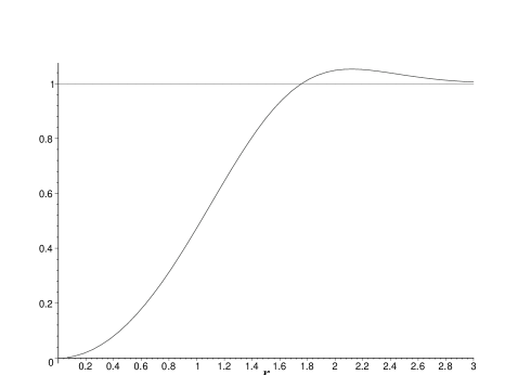
Figure 1. The 1-dimensional limit pair correlation function $\kappa_{11}$

For $\dim M=2$, the simultaneous scaled zeros of a random pair $(s_{1},s_{2})$ of sections still exhibit a mild repulsion ($\lim_{r\to 0}\kappa_{22}(r)=\frac{3}{4}$), as illustrated in Figure 2 below.

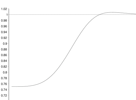
Figure 2. The limit pair correlation function $\kappa_{22}$

The function $\kappa_{mm}(r)$ can be interpreted as the normalized conditional probability of finding a zero near a point $z^{1}$ given that there is a zero at a second point a scaled distance $r$ from $z^{1}$ (in the case of discrete zeros in $m$ dimensions). The above graphs show that for dimensions 1 and 2, there is a unique scaled distance where this probability is maximized. It would be interesting to explore the dependence of the correlations on the dimension. To ask one concrete question, do the simultaneous scaled zeros in the point case become more and more independent in the sense that $\kappa_{mm}(r)\to 1$ as the dimension $m\to\infty$?

When $k<m$, the zero sets are subvarieties of positive dimension $m-k$; in this case the expected volume of the zero set in a small spherical shell of radius $r$ and thickness $\varepsilon$ about a point in the zero set must be $\sim\varepsilon r^{2m-2k-1}$. Hence we have $\kappa_{km}(r)\sim r^{-2k}$, for small $r$. The graph of the limit correlation function for the case $m=2,k=1$ is given in Figure 3 below.

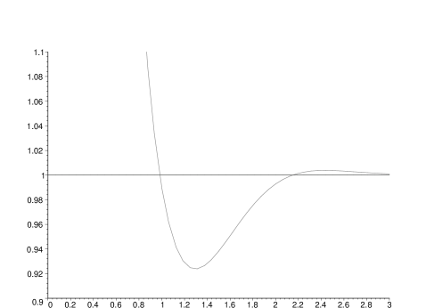
Figure 3. The limit pair correlation function $\kappa_{12}$

To end this introduction, we would like to link our methods and results at least heuristically to a long tradition of (largely heuristic) results on universality and scaling in statistical mechanics (cf. [FFS]). One may view the rescaling transformation on $U$ as generating a renormalization group. The intuitive picture in statistical mechanics is that the renormalization group should carry a given system (read “$L\to M$”) to the fixed point of the renormalization group, i.e. to the scale invariant situation. We observe that the local rescaling of $U$ is nothing other than the Heisenberg dilations $\delta_{\sqrt{N}}$ on ${\bf H}^{m}_{\rm red}$. Since these dilations are automorphisms of the (unreduced) Heisenberg group, the Szegö kernel of ${\bf H}^{m}$ is invariant under these dilations; i.e., it is the fixed point of the renormalization group. As predicted by this intuitive picture, we find that in the scaling limit all the invariants of the line bundle, in particular its zero-point correlation functions, are drawn to their values for the fixed point system (read “Heisenberg model”).

1. Notation

We begin with some notation and basic properties of sections of holomorphic line bundles, their zero sets, Szegö kernels, and Gaussian measures. We also provide two examples that will serve as model cases for studying correlations of zeros of sections of line bundles in the high power limit.

1.1. Sections of holomorphic line bundles

In this section, we introduce the basic complex analytic objects: holomorphic sections and the currents of integration over their zero sets. We also introduce Gaussian probability measures on spaces of holomorphic sections. For background in complex geometry, we refer to [GH].

Let $M$ be a compact complex manifold and let $L\to M$ be a holomorphic line bundle with a smooth Hermitian metric $h$; its curvature 2-form $\Theta_{h}$ is given locally by

(1) $$\Theta_{h}=-\partial\bar{\partial}\log\|e_{L}\|_{h}^{2}\;,$$

where $e_{L}$ denotes a local holomorphic frame (= nonvanishing section) of $L$ over an open set $U\subset M$, and $\|e_{L}\|_{h}=h(e_{L},e_{L})^{1/2}$ denotes the $h$-norm of $e_{L}$. We say that $(L,h)$ is positive if the (real) 2-form $\omega=\frac{\sqrt{-1}}{2}\Theta_{h}$ is positive, i.e., if $\omega$ is a Kähler form. We henceforth assume that $(L,h)$ is positive, and we give $M$ the Hermitian metric corresponding to the Kähler form $\omega$ and the induced Riemannian volume form

(2) $$dV_{M}=\frac{1}{m!}\omega^{m}\;.$$

Since $\frac{1}{\pi}\omega$ is a de Rham representative of the Chern class $c_{1}(L)\in H^{2}(M,{\mathbb{R}})$, the volume of $M$ equals $\frac{\pi^{m}}{m!}c_{1}(L)^{m}$.

The space $H^{0}(M,L^{N})$ of global holomorphic sections of $L^{N}=L\otimes\cdots\otimes L$ is a finite dimensional complex vector space. (Its dimension, given by the Riemann-Roch formula for large $N$, grows like $N^{m}$. By the Kodaira embedding theorem, the global sections of $L^{N}$ give an embedding into a projective space for $N\gg 0$, and hence $M$ is a projective algebraic manifold.) The metric $h$ induces Hermitian metrics $h^{N}$ on $L^{N}$ given by $\|s^{\otimes N}\|_{h^{N}}=\|s\|_{h}^{N}$. We give $H^{0}(M,L^{N})$ the Hermitian inner product

(3) $$\langle s_{1},s_{2}\rangle=\int_{M}h^{N}(s_{1},s_{2})dV_{M}\quad\quad(s_{1},s_{2}\in H^{0}(M,L^{N})\,)\;,$$

and we write $|s|=\langle s,s\rangle^{1/2}$.

We now explain our concept of a “random section.” We are interested in expected values and correlations of zero sets of $k$-tuples of holomorphic sections of powers $L^{N}$. Since the zeros do not depend on constant factors, we could suppose our sections lie in the unit sphere in $H^{0}(M,L^{N})$ with respect to the Hermitian inner product (3), and we pick random sections with respect to the spherical measure. Equivalently, we could suppose that $s$ is a random element of the projectivization ${\mathbb{P}}H^{0}(M,L^{N})$. Another equivalent approach is to use Gaussian measures on the entire space $H^{0}(M,L^{N})$. We shall use the third approach, since Gaussian measures seem the best for calculations. Precisely, we give $H^{0}(M,L^{N})$ the complex Gaussian probability measure

(4) $$d\nu_{N}(s)=\frac{1}{\pi^{m}}e^{-|c|^{2}}dc\,,\qquad s=\sum_{j=1}^{d_{N}}c_{j}S_{j}^{N}\,,$$

where $\{S_{j}^{N}\}$ is an orthonormal basis for $H^{0}(M,L^{N})$ and $dc$ is $2d_{N}$-dimensional Lebesgue measure. This Gaussian is characterized by the property that the $2d_{N}$ real variables $\Re c_{j},\Im c_{j}$ ($j=1,\dots,d_{N}$) are independent random variables with mean 0 and variance ${\frac{1}{2}}$; i.e.,

$${\mathbf{E}}\,c_{j}=0,\quad{\mathbf{E}}\,c_{j}c_{k}=0,\quad{\mathbf{E}}\,c_{j}\bar{c}_{k}=\delta_{jk}\,.$$

Here and throughout this paper, ${\mathbf{E}}\,$ denotes expectation.

In general, a complex Gaussian measure (with mean 0) on a finite dimensional complex vector space $V$ is a measure $\nu$ of the form (4), where the $c_{j}$ are the coordinates with respect to some basis. Explicitly, the complex Gaussian measures on ${\mathbb{C}}^{m}$ are the probability measures of the form

(5) $$\frac{e^{-\langle\Delta^{-1}z,z\rangle}}{\pi^{m}\det\Delta}dz$$

where $\Delta=(\Delta^{j}_{k})$ is a positive definite Hermitian matrix and

$$\langle\zeta,z\rangle=\zeta\cdot\bar{z}=\sum_{q=1}^{m}\zeta_{q}\bar{z}_{q}$$

denotes the standard Hermitian inner product in ${\mathbb{C}}^{m}$. For the Gaussian measure (5), we have

(6) $${\mathbf{E}}\,(z_{j}z_{k})=0,\qquad{\mathbf{E}}\,(z_{j}\bar{z}_{k})=\Delta^{j}_{k}\,.$$

If $\nu$ is a complex Gaussian on $V$ and $\tau:V\to\widetilde{V}$ is a surjective linear transformation, then $\tau_{*}\nu$ is a complex Gaussian on $\widetilde{V}$. In particular, if $\widetilde{V}={\mathbb{C}}^{m}$, then, $\tau_{*}\nu$ is of the form (5), where the covariance matrix $\Delta$ is given by (6) with $z_{j}=z_{j}\circ\tau:V\to{\mathbb{C}}$.

We shall consider the space $\mathcal{S}=H^{0}(M,L^{N})^{k}$ ($1\leq k\leq m$) with the probability measure $d\mu=d\nu\times\cdots\times d\nu$, which is also Gaussian. Picking a random element of $\mathcal{S}$ means picking $k$ sections of $H^{0}(M,L^{N})$ independently and at random. For $s=(s_{1},\dots,s_{k})\in\mathcal{S}$, we let

$$Z_{s}=\{z\in M:s_{1}(z)=\cdots=s_{k}(z)=0\}$$

denote the zero set of $s$. Note that if $N$ is sufficiently large so that $L^{N}$ is base point free, then for $\mu$-a.a. $s\in\mathcal{S}$, we have ${\operatorname{codim\,}}Z_{s}=k$. (Indeed, the set of $s$ where ${\operatorname{codim\,}}Z_{s}<k$ is a proper algebraic subvariety of $H^{0}(M,L^{N})^{k}$. In fact, by Bertini’s theorem, the $Z_{s}$ are smooth submanifolds of complex dimension $m-k$ for almost all $s$, provided $N$ is large enough so that the global sections of $L^{N}$ give a projective embedding of $M$, but we do not need this fact here.) For these $s$, we let $|Z_{s}|$ denote Riemannian $(2m-2k)$-volume along the regular points of $Z_{s}$, regarded as a measure on $M$:

(7) $$(|Z_{s}|,\varphi)=\int_{Z_{s}^{\rm reg}}\varphi d{\operatorname{Vol}}_{2m-2k}=\frac{1}{(m-k)!}\int_{Z_{s}^{\rm reg}}\varphi\omega^{m-k}\,.$$

It was shown by Lelong [Le] (see also [GH]) that the integral in (7) converges. (In fact, $|Z_{s}|$ can be regarded as the total variation measure of the closed current of integration over $Z_{s}$.) We regard $|Z_{s}|$ as a measure-valued random variable on the probability space $(\mathcal{S},d\mu)$; i.e., for each test function $\varphi\in\mathcal{C}^{0}(M)$, $(|Z_{s}|,\varphi)$ is a complex-valued random variable.

1.2. Szegö kernels

As in [Ze, SZ] we now lift the analysis of holomorphic sections over $M$ to a certain $S^{1}$ bundle $X\to M$. This is a useful approach to the asymptotics of powers of line bundles and goes back at least to [BG].

We let $L^{*}$ denote the dual line bundle to $L$, and we consider the circle bundle $X=\{\lambda\in L^{*}:\|\lambda\|_{h^{*}}=1\}$, where $h^{*}$ is the norm on $L^{*}$ dual to $h$. Let $\pi:X\to M$ denote the bundle map; if $v\in L_{z}$, then $\|v\|_{h}=|(\lambda,v)|$, $\lambda\in X_{z}=\pi^{-1}(z)$. Note that $X$ is the boundary of the disc bundle $D=\{\lambda\in L^{*}:\rho(\lambda)>0\}$, where $\rho(\lambda)=1-\|\lambda\|^{2}_{h^{*}}$. The disc bundle $D$ is strictly pseudoconvex in $L^{*}$, since $\Theta_{h}$ is positive, and hence $X$ inherits the structure of a strictly pseudoconvex CR manifold. Associated to $X$ is the contact form $\alpha=-i\partial\rho|_{X}=i\bar{\partial}\rho|_{X}$. We also give $X$ the volume form

(8) $$dV_{X}=\frac{1}{m!}\alpha\wedge(d\alpha)^{m}=\alpha\wedge\pi^{*}dV_{M}\,.$$

The setting for our analysis of the Szegö kernel is the Hardy space $\mathcal{H}^{2}(X)\subset\mathcal{L}^{2}(X)$ of square-integrable CR functions on $X$, i.e., functions that are annihilated by the Cauchy-Riemann operator $\bar{\partial}_{b}$ (see [St, pp. 592–594]) and are $\mathcal{L}^{2}$ with respect to the inner product

(9) $$\langle F_{1},F_{2}\rangle=\frac{1}{2\pi}\int_{X}F_{1}\overline{F_{2}}dV_{X}\,,\quad F_{1},F_{2}\in\mathcal{L}^{2}(X)\,.$$

Equivalently, $\mathcal{H}^{2}(X)$ is the space of boundary values of holomorphic functions on $D$ that are in $\mathcal{L}^{2}(X)$. We let $r_{\theta}x=e^{i\theta}x$ ($x\in X$) denote the $S^{1}$ action on $X$ and denote its infinitesimal generator by $\frac{\partial}{\partial\theta}$. The $S^{1}$ action on $X$ commutes with $\bar{\partial}_{b}$; hence $\mathcal{H}^{2}(X)=\bigoplus_{N=0}^{\infty}\mathcal{H}^{2}_{N}(X)$ where $\mathcal{H}^{2}_{N}(X)=\{F\in\mathcal{H}^{2}(X):F(r_{\theta}x)=e^{iN\theta}F(x)\}$. A section $s$ of $L$ determines an equivariant function $\hat{s}$ on $L^{*}$ by the rule $\hat{s}(\lambda)=\left(\lambda,s(z)\right)$ ($\lambda\in L^{*}_{z},z\in M$). It is clear that if $\tau\in{\mathbb{C}}$ then $\hat{s}(z,\tau\lambda)=\tau\hat{s}$. We henceforth restrict $\hat{s}$ to $X$ and then the equivariance property takes the form $\hat{s}(r_{\theta}x)=e^{i\theta}\hat{s}(x)$. Similarly, a section $s_{N}$ of $L^{N}$ determines an equivariant function $\hat{s}_{N}$ on $X$: put

$$\hat{s}_{N}(\lambda)=\left(\lambda^{\otimes N},s_{N}(z)\right)\,,\quad\lambda\in X_{z}\,,$$

where $\lambda^{\otimes N}=\lambda\otimes\cdots\otimes\lambda$; then $\hat{s}_{N}(r_{\theta}x)=e^{iN\theta}\hat{s}_{N}(x)$. The map $s\mapsto\hat{s}$ is a unitary equivalence between $H^{0}(M,L^{N})$ and $\mathcal{H}^{2}_{N}(X)$. (This follows from (8)–(9) and the fact that $\alpha=d\theta$ along the fibers of $\pi:X\to M$.)

We let $\Pi_{N}:\mathcal{L}^{2}(X)\rightarrow\mathcal{H}^{2}_{N}(X)$ denote the orthogonal projection. The Szegö kernel $\Pi_{N}(x,y)$ is defined by

(10) $$\Pi_{N}F(x)=\int_{X}\Pi_{N}(x,y)F(y)dV_{X}(y)\,,\quad F\in\mathcal{L}^{2}(X)\,.$$

It can be given as

(11) $$\Pi_{N}(x,y)=\sum_{j=1}^{d_{N}}\widehat{S}_{j}^{N}(x)\overline{\widehat{S}_{j}^{N}(y)}\,,$$

where $S_{1}^{N},\dots,S_{d_{N}}^{N}$ form an orthonormal basis of $H^{0}(M,L^{N})$. Pick a local holomorphic frame $e_{L}$ for $L$ over an open subset $U\subset M$, let $e_{L}^{*}$ denote the dual frame, and write $h(z)=h(e_{L}(z),e_{L}(z))=\|e_{L}\|_{h}^{2}$. The map $(z,e^{i\theta})\mapsto e^{i\theta}h(z)^{1/2}e_{L}^{*}(z)$ gives an isomorphism $U\times S^{1}\approx\pi^{-1}(U)\subset X$, and we use the coordinates $(z,\theta)$ to identify points of $\pi^{-1}(U)$. For $s\in H^{0}(M,L^{N})$, we have

(12) $$\hat{s}(z,\theta)=\left\langle s(z),e^{iN\theta}h(z)^{N/2}e^{*}_{L}(z)\right\rangle=e^{iN\theta}h(z)^{N/2}f(z),\quad s=fe_{L}^{\otimes N}\,.$$

Although the Szegö kernel is defined on $X$, its absolute value is well-defined on $M$ as follows: writing $S_{j}^{N}=f^{N}_{j}e_{L}^{\otimes N}$, we have

(13) $$\Pi_{N}(z,\theta;w,\varphi)=e^{iN(\theta-\varphi)}\Pi_{N}(z,0;w,0)=e^{iN(\theta-\varphi)}h(z)^{N/2}h(w)^{N/2}\sum_{j=1}^{d_{N}}f^{N}_{j}(z)\overline{f^{N}_{j}(w)}\,,$$

for $z,w\in U$. (Here we may take $U$ to be the disjoint union of connected neighborhoods of $z$ and $w$, if $z$ is not close to $w$.) Thus we can write

$$|\Pi_{N}(z,w)|=|\Pi_{N}(z,0;w,0)|\,,$$

which is independent of the choice of local frame $e_{L}$. On the diagonal we have

$$\Pi_{N}(z,z)=\Pi_{N}(z,\theta;z,\theta)=\sum_{j=1}^{d_{N}}\|S_{j}^{N}(z)\|_{h^{N}}\,.$$

The Hermitian connection $\nabla$ on $L$ induces the decomposition $T_{X}=T_{X}^{H}\oplus T_{X}^{V}$ into horizontal and vertical components, and we let $t^{H}$ denote the horizontal lift (to $X$) of a vector field $t$ in $M$. We consider the horizontal operators on $X$:

$$d_{z_{q}}^{H}\buildrel\operatorname{def}\over{=}d_{(\partial/\partial z_{q})^{H}}\,,\quad d_{\bar{z}_{q}}^{H}\buildrel\operatorname{def}\over{=}d_{(\partial/\partial\bar{z}_{q})^{H}}\,,$$

where $z_{1},\dots,z_{m},\theta$ denote local coordinates on $X$. We note that

(14) $$d_{z_{q}}^{H}\hat{s}=(\nabla^{N}_{z_{q}}s)\raisebox{2.0pt}{$\widehat{\ }$}\;,\quad s\in H^{0}(M,L^{N})\,,$$

where $\nabla^{N}$ is the induced connection on $L^{N}$. We then have

$$d^{H}_{z_{q}}\Pi_{N}(z,\theta;w,\varphi) = \sum_{j=1}^{d_{N}}\left(\nabla^{N}_{z_{q}}S_{j}^{N}\right)\raisebox{2.0pt}{$\widehat{\ }$}(x)\overline{\widehat{S}_{j}^{N}(y)}$$

$$= e^{iN(\theta-\varphi)}h(z)^{N/2}h(w)^{N/2}\sum_{j=1}^{d_{N}}f^{N}_{j;q}(z)\overline{f^{N}_{j}(w)}\,,$$

$$d^{H}_{z_{p}}d^{H}_{\bar{w}_{q}}\Pi_{N}(z,\theta;w,\varphi) = \sum_{j=1}^{d_{N}}\left(\nabla^{N}_{z_{p}}S_{j}^{N}\right)\raisebox{2.0pt}{$\widehat{\ }$}(x)\overline{\left(\nabla^{N}_{w_{q}}S_{j}^{N}\right)\raisebox{2.0pt}{$\widehat{\ }$}(y)}$$

$$= e^{iN(\theta-\varphi)}h(z)^{N/2}h(w)^{N/2}\sum_{j=1}^{d_{N}}f^{N}_{j;p}(z)\overline{f^{N}_{j;q}(w)}\,,$$

$$\qquad\nabla^{N}_{z_{q}}=\nabla^{N}_{\partial/\partial z_{q}}\,,\quad f^{N}_{j;q}=\frac{\partial f}{\partial z_{q}}+Nf^{N}_{j}h^{-1}\frac{\partial h}{\partial z_{q}}\,.$$

We can also use (12) and (14) to describe the horizontal lift in local coordinates:

(16) $$d^{H}_{z_{q}}=\frac{\partial}{\partial z_{q}}-\frac{i}{2}\frac{\partial\log h}{\partial z_{q}}\frac{\partial}{\partial\theta}\,.$$

1.3. Model examples

In two special cases we can work out the Szegö kernels and their derivatives explicitly, namely for the hyperplane section bundle over ${\mathbb{C}}{\mathbb{P}}^{m}$ and for the Heisenberg bundle over ${\mathbb{C}}^{m}$, i.e. the trivial line bundle with curvature equal to the standard symplectic form on ${\mathbb{C}}^{m}$. These cases will be important after we have proven universality, since scaling limits of correlation functions for all line bundles coincide with those of the model cases.

In fact, the two models are locally equivalent in the CR sense. In the case of ${\mathbb{C}}{\mathbb{P}}^{m}$, the circle bundle $X$ is the $2m+1$ sphere $S^{2m+1}$, which is the boundary of the unit ball $B^{2m+2}\subset{\mathbb{C}}^{m+1}$. In the case of ${\mathbb{C}}^{m}$, the circle bundle is the reduced Heisenberg group ${\bf H}^{m}_{\rm red}$, which is a discrete quotient of the simply connected Heisenberg group ${\mathbb{C}}^{m}\times{\mathbb{R}}$. As is well-known, the latter is equivalent (in the CR and contact sense) to the boundary of $B^{2m+2}$ ([St]).

1.3.1. ${\operatorname{SU}}(m+1)$-polynomials

For our first example, we let $M={\mathbb{C}}{\mathbb{P}}^{m}$ and take $L$ to be the hyperplane section bundle $\mathcal{O}(1)$. Sections $s\in H^{0}({\mathbb{C}}{\mathbb{P}}^{m},\mathcal{O}(1))$ are linear functions on ${\mathbb{C}}^{m+1}$; the zero divisors $Z_{s}$ are projective hyperplanes. The line bundle $\mathcal{O}(1)$ carries a natural metric $h_{{\operatorname{FS}}}$ given by

(17) $$\|s\|_{h_{{\operatorname{FS}}}}([w])=\frac{|(s,w)|}{|w|}\;,\quad\quad w=(w_{0},\dots,w_{m})\in{\mathbb{C}}^{m+1}\;,$$

for $s\in{\mathbb{C}}^{m+1*}\equiv H^{0}({\mathbb{C}}{\mathbb{P}}^{m},\mathcal{O}(1))$, where $|w|^{2}=\sum_{j=0}^{m}|w_{j}|^{2}$ and $[w]\in{\mathbb{C}}{\mathbb{P}}^{m}$ is the complex line through $w$. The Kähler form on ${\mathbb{C}}{\mathbb{P}}^{m}$ is the Fubini-Study form

(18) $$\omega_{{\operatorname{FS}}}=\frac{\sqrt{-1}}{2}\Theta_{h_{{\operatorname{FS}}}}=\frac{\sqrt{-1}}{2}\partial\bar{\partial}\log|w|^{2}\,.$$

The dual bundle $L^{*}=\mathcal{O}(-1)$ is the affine space ${\mathbb{C}}^{m+1}$ with the origin blown up, and $X=S^{2m+1}\subset{\mathbb{C}}^{m+1}$. The $N$-th tensor power of $\mathcal{O}(1)$ is denoted $\mathcal{O}(N)$. Elements $s_{N}\in H^{0}({\mathbb{C}}{\mathbb{P}}^{m},\mathcal{O}(N))$ are homogeneous polynomials on ${\mathbb{C}}^{m+1}$ of degree $N$, and $\hat{s}_{N}=s_{N}|_{S^{2m-1}}$. The monomials

(19) $$s^{N}_{J}=\left[\frac{(N+m)!}{\pi^{m}j_{0}!\cdots j_{m}!}\right]^{\frac{1}{2}}z^{J}\,,\quad z^{J}=z_{0}^{j_{0}}\cdots z_{m}^{j_{m}},\quad\quad J=(j_{0},\ldots,j_{m}),\ |J|=N$$

form an orthonormal basis for $H^{0}({\mathbb{C}}{\mathbb{P}}^{m},\mathcal{O}(N))$. (See [SZ, §4.2]; the extra factor $\left(\frac{m!}{\pi^{m}}\right)^{1/2}$ in (19) comes from the fact that here ${\mathbb{C}}{\mathbb{P}}^{m}$ has the usual volume $\frac{\pi^{m}}{m!}$, whereas in [SZ], the volume of ${\mathbb{C}}{\mathbb{P}}^{m}$ is normalized to be 1.) Hence the Szegö kernel for $\mathcal{O}(N)$ is given by

(20) $$\Pi_{N}(x,y)=\sum_{J}\frac{(N+m)!}{\pi^{m}j_{0}!\cdots j_{m}!}x^{J}\bar{y}^{J}=\frac{(N+m)!}{\pi^{m}N!}\langle x,y\rangle^{N}\,.$$

Note that

$$\Pi(x,y)=\sum_{N=1}^{\infty}\Pi_{N}(x,y)=\frac{m!}{\pi^{m}}(1-\langle x,y\rangle)^{-(m+1)}=2\pi\times[\mbox{classical Szeg\"{o} kernel on}\ S^{2m+1}]\,.$$

(The factor $2\pi$ is due to our normalization (9).)

1.3.2. The Heisenberg model

Our second example is the linear model ${\mathbb{C}}^{m}\times{\mathbb{C}}\to{\mathbb{C}}^{m}$ for positive line bundles $L\to M$ over Kähler manifolds and their associated Szegö kernels. It is most illuminating to consider the associated principal $S^{1}$ bundle ${\mathbb{C}}^{m}\times S^{1}\to{\mathbb{C}}^{m}$, which may be identified with the boundary of the disc bundle $D\subset L^{*}$ in the dual line bundle. This $S^{1}$ bundle is the reduced Heisenberg group ${\bf H}_{\rm red}^{m}$ (cf. [Fo], p. 23).

Let us recall its definition and properties. We start with the usual (simply connected) Heisenberg group ${\bf H}^{m}$ (cf. [Fo] [St]; note that different authors differ by factors of $2$ and $\pi$ in various definitions). It is the group ${\mathbb{C}}^{m}\times{\mathbb{R}}$ with group law

$$(\zeta,t)\cdot(\eta,s)=(\zeta+\eta,t+s+\Im(\zeta\cdot\bar{\eta})).$$

The identity element is $(0,0)$ and $(\zeta,t)^{-1}=(-\zeta,-t)$. Abstractly, the Lie algebra of ${\bf H}_{m}$ is spanned by elements $Z_{1},\dots,Z_{m},\bar{Z}_{1},\dots,\bar{Z}_{m},T$ satisfying the canonical commutation relations $[Z_{j},\bar{Z}_{k}]=-i\delta_{jk}T$ (all other brackets zero). Below we will select such a basis of left invariant vector fields.

${\bf H}^{m}$ is a strictly convex CR manifold which may be embedded in ${\mathbb{C}}^{m+1}$ as the boundary of a strictly pseudoconvex domain, namely the upper half space $\mathcal{U}^{m}:=\{z\in{\mathbb{C}}^{m+1}:\Im z_{m+1}>{\frac{1}{2}}\sum_{j=1}^{m}|z_{j}|^{2}\}$. The boundary of $\mathcal{U}^{m}$ equals $\partial\mathcal{U}^{m}=\{z\in{\mathbb{C}}^{m+1}:\Im z_{m+1}={\frac{1}{2}}\sum_{j=1}^{m}|z_{j}|^{2}\}$. ${\bf H}^{m}$ acts simply transitively on $\partial\mathcal{U}^{m}$ (cf. [St], XII), and we get an identification of ${\bf H}^{m}$ with $\partial\mathcal{U}^{m}$ by:

$$[\zeta,t]\to(\zeta,t+i|\zeta|^{2})\in\partial\mathcal{U}^{m}.$$

The Szegö projector of ${\bf H}^{m}$ is the operator $\Pi:\mathcal{L}^{2}({\bf H}^{m})\to\mathcal{H}^{2}({\bf H}^{m})$ of orthogonal projection onto boundary values of holomorphic functions on $\mathcal{U}^{m}$ which lie in $\mathcal{L}^{2}$. The kernel of $\Pi$ is given by (cf. [St], XII §2 (29))

$$\Pi(x,y)=K(y^{-1}x),\;\;\;\;\;\;\;K(x)=-C_{m}\frac{\partial}{\partial t}[t+i|\zeta|^{2}]^{-m}\in\mathcal{D}^{\prime}({\mathbf{H}}^{m})\,.$$

The linear model for the principal $S^{1}$ bundle described in §1.2 is the so-called reduced Heisenberg group ${\bf H}^{m}_{\rm red}={\bf H}^{m}/\{(0,2\pi k):k\in{\mathbb{Z}}\}={\mathbb{C}}^{m}\times S^{1}$ with group law

$$(\zeta,e^{it})\cdot(\eta,e^{is})=(\zeta+\eta,e^{i(t+s+\Im(\zeta\cdot\bar{\eta}))}).$$

It is the principal $S^{1}$ bundle over ${\mathbb{C}}^{m}$ associated to the line bundle $L_{\mathbf{H}}={\mathbb{C}}^{m}\times{\mathbb{C}}$. The metric on $L_{\mathbf{H}}$ with curvature $\Theta=\partial\bar{\partial}|z|^{2}$ is given by setting $h_{\mathbf{H}}(z)=e^{-|z|^{2}}$; i.e., $|f|_{h_{\mathbf{H}}}=|f|e^{-|z|^{2}/2}$. The reduced Heisenberg group ${\bf H}^{m}_{\rm red}$ may be viewed as the boundary of the dual disc bundle $D\subset L^{*}_{\mathbf{H}}$ and hence is a strictly pseudoconvex CR manifold.

It seems most natural to approach the analysis of the Szegö kernels on ${\bf H}^{m}_{\rm red}$ from the representation-theoretic point of view. Let us begin with the case $N=1$. We thus consider the space $\mathcal{V}_{1}\subset\mathcal{L}^{2}({\bf H}^{m}_{\rm red})$ of functions $f$ satisfying $\frac{1}{i}\frac{\partial}{\partial\theta}f=f$, which forms a (reducible) representation of ${\bf H}^{m}_{\rm red}$ with central character $e^{i\theta}$. By the Stone-von Neumann theorem there exists a unique (up to equivalence) representation $(V_{1},\rho_{1})$ with this character and by the Plancherel theorem, $\mathcal{V}_{1}\cong V_{1}\otimes V_{1}^{*}$.

The space of CR functions in $\mathcal{V}_{1}$ is an irreducible invariant subspace. Here, by CR functions we mean the functions satisfying the left-invariant Cauchy-Riemann equations $\bar{Z}^{L}_{q}f=0$ on ${\bf H}^{m}_{\rm red}$. Here, $\{\bar{Z}^{L}_{q}\}$ denotes a basis of the left-invariant anti-holomorphic vector fields on ${\bf H}^{m}_{\rm red}$. Let us recall their definition: we first equip ${\bf H}^{m}_{\rm red}$ with its left-invariant contact form $\alpha^{L}=\sum_{q}(u_{q}dv_{q}-v_{q}du_{q})+d\theta$ ($\zeta=u+iv$). The left-invariant CR holomorphic (resp. anti-holomorphic) vector fields $Z_{q}^{L}$ (resp. $\bar{Z}_{q}^{L}$) are the horizontal lifts of the vector fields $\frac{\partial}{\partial z_{q}}$ (resp. $\frac{\partial}{\partial\bar{z}_{q}}$) with respect to $\alpha^{L}$. They span the left-invariant CR structure of ${\bf H}^{m}_{\rm red}$ and the $Z_{q}^{L}$ obviously have the form $Z_{q}^{L}=\frac{\partial}{\partial z_{q}}+A\frac{\partial}{\partial\theta}$ where the coefficient $A$ is determined by the condition $\alpha^{L}(Z_{q}^{L})=0$. An easy calculation gives:

$$Z_{q}^{L}=\frac{\partial}{\partial z_{q}}+\frac{i}{2}\bar{z}_{q}\frac{\partial}{\partial\theta},\;\;\;\;\bar{Z}^{L}_{q}=\frac{\partial}{\partial\bar{z}_{q}}-\frac{i}{2}z_{q}\frac{\partial}{\partial\theta}.$$

The vector fields $\{\frac{\partial}{\partial\theta},Z_{q}^{L},\bar{Z}_{q}^{L}\}$ span the Lie algebra of ${\bf H}^{m}_{\rm red}$ and satisfy the canonical commutation relations above.

We then define the Hardy space $\mathcal{H}^{2}({\bf H}^{m}_{\rm red})$ of CR holomorphic functions, i.e. solutions of $\bar{Z}_{q}^{L}f=0$, which lie in $\mathcal{L}^{2}({\bf H}^{m}_{\rm red})$. We also put $\mathcal{H}^{2}_{1}=\mathcal{V}_{1}\cap\mathcal{H}^{2}({\bf H}^{m}_{\rm red}).$ The group ${\bf H}^{m}_{\rm red}$ acts by left translation on $\mathcal{H}^{2}_{1}$. The generators of this representation are the right-invariant vector fields $Z_{q}^{R},\bar{Z}_{q}^{R}$ together with $\frac{\partial}{\partial\theta}$. They are horizontal with respect to the right-invariant contact form $\alpha^{R}=\sum_{q}(u_{q}dv_{q}-v_{q}du_{q})-d\theta$ and are given by:

$$Z_{q}^{R}=\frac{\partial}{\partial z_{q}}-\frac{i}{2}\bar{z}_{q}\frac{\partial}{\partial\theta},\;\;\;\;\bar{Z}^{R}_{q}=\frac{\partial}{\partial\bar{z}_{q}}+\frac{i}{2}z_{q}\frac{\partial}{\partial\theta}\,.$$

In physics terminology, $Z_{q}^{R}$ is known as an annihilation operator and $\bar{Z}_{q}^{R}$ is a creation operator.

The representation $\mathcal{H}^{2}_{1}$ is irreducible and may be identified with the Bargmann-Fock space of entire holomorphic functions on ${\mathbb{C}}^{m}$ which are square integrable relative to $e^{-|z|^{2}}$ (or equivalently, holomorphic sections of the trivial line bundle $L_{\mathbf{H}}={\mathbb{C}}^{m}\times{\mathbb{C}}$ mentioned above, with hermitian metric $h_{\mathbf{H}}=e^{-|z|^{2}}$). The identification goes as follows: the function $\varphi_{0}(z,\theta):=e^{i\theta}e^{-|z|^{2}/2}$ is CR holomorphic and is also the ground state for the right invariant “annihilation operator;” i.e., it satisfies

$$\bar{Z}^{L}_{q}\varphi_{0}(z,\theta)=0=Z_{q}^{R}\varphi_{0}(z,\theta)\,.$$

Any element $F(z,\theta)$ of $\mathcal{H}^{2}_{1}$ may be written in the form $F(z,\theta)=f(z)\varphi_{0}.$ Then $\bar{Z}^{L}_{q}F=(\frac{\partial}{\partial\bar{z}_{q}}f)\varphi_{0}$, so that $F$ is CR if and only if $f$ is holomorphic. Moreover, $F\in\mathcal{L}^{2}({\bf H}^{m}_{\rm red})$ if and only if $f$ is square integrable relative to $e^{-|z|^{2}}$.

The Szegö kernel $\Pi_{1}^{\mathbf{H}}(z,\theta,w,\varphi)$ of ${\bf H}^{m}_{\rm red}$ is by definition the orthogonal projection from $\mathcal{L}({\bf H}^{m}_{\rm red})$ to $H^{2}_{1}.$ As will be seen below, $\Pi_{1}^{\mathbf{H}}(z,\theta,w,\varphi)=\frac{1}{\pi_{m}}e^{i(\theta-\varphi)}e^{(z\cdot\bar{w}-{\frac{1}{2}}|z|^{2}-{\frac{1}{2}}|w|^{2})}$, which is the left translate of $\varphi_{0}$ by $(-w,-\varphi)$. In the physics terminology it is the coherent state associated to the phase space point $w.$

So far we have set $N=1$, but the story is very similar for any $N$. We define $\mathcal{H}^{2}_{N}$ as the space of square- integrable CR functions transforming by $e^{iN\theta}$ under the central $S^{1}$. By the Stone-von Neumann theorem there is a unique irreducible $V_{N}$ with this central character. The main difference to the case $N=1$ is that $\mathcal{H}^{2}_{N}$ is of multiplicity $N^{m}$. The Szegö kernel $\Pi_{N}^{\mathbf{H}}(x,y)$ is the orthogonal projection to $\mathcal{H}^{2}_{N}$ and is given by the dilate of $\Pi^{\mathbf{H}}_{1}$. Thus,

$$\Pi_{N}^{\mathbf{H}}(x,y)=\frac{1}{\pi^{m}}N^{m}e^{iN(\theta-\varphi)}e^{N(z\cdot\bar{w}-{\frac{1}{2}}|z|^{2}-{\frac{1}{2}}|w|^{2})}.$$

To prove these formulae for the Szegö kernels, we observe that the reduced Szegö kernels are obtained by projecting the Szegö kernel on ${\bf H}^{m}$ to ${\bf H}_{\rm red}^{m}$ as an automorphic kernel, i.e.

$$\Pi^{\mathbf{H}}(x,y)=\sum_{n\in{\mathbb{Z}}}\Pi(x,y\cdot(0,2\pi n)).$$

Let us write $x=(z,\theta),y=(w,\varphi)$. Then the $N$-th Fourier component $\Pi^{\mathbf{H}}_{N}(x,y)$ of $\Pi^{\mathbf{H}}$, i.e. the projection onto square integrable holomorphic sections of $L^{N}$, is given by:

$$\Pi^{\mathbf{H}}_{N}(x,y) = \int_{{\mathbb{R}}}e^{-iNt}\Pi(e^{it}x,y)dt\ =\ \int_{{\mathbb{R}}}e^{-iNt}K(e^{it}y^{-1}x)dt$$

$$= \int_{{\mathbb{R}}}e^{-iNt}K(z-w,e^{i(\theta-\varphi+t+\Im(z\cdot\bar{w})})dt\,.$$

Here we abbreviated the element $(0,e^{it})$ by $e^{it}$. Change variables $t\mapsto t-\theta+\varphi-\Im(z\cdot\bar{w})$ to get

$$\begin{array}[]{l}\Pi^{\mathbf{H}}_{N}(x,y)=e^{iN(\theta-\varphi)}e^{iN\Im(z\cdot\bar{w}})\int_{{\mathbb{R}}}e^{-iNt}K(z-w,t)dt\\ \\ =e^{iN(\theta-\varphi)}e^{iN\Im(z\cdot\bar{w})}\hat{K}_{t}(z-w,N)\end{array}$$

where $\hat{K}_{t}$ is the Fourier transform of $K$ with respect to the $t$ variable. By [St, p. 585], the full ${\mathbb{R}}^{2m}\times{\mathbb{R}}$ Fourier transform of $K$ is given by $\hat{K}(z,N)=C^{\prime}_{m}e^{-|z|^{2}/2N}$, so by taking the inverse Fourier transform in the $z$ variable we get the Fourier transform just in the $t$ variable:

(21) $$\Pi^{\mathbf{H}}_{N}(x,y)=\frac{1}{\pi^{m}}N^{m}e^{iN(\theta-\varphi)}e^{iN\Im(z\cdot\bar{w})}e^{-{\frac{1}{2}}N|z-w|^{2}}.$$

(Our constant factor $\frac{1}{\pi^{m}}$ in (21) is determined by the condition that $\Pi_{N}^{\mathbf{H}}$ is an orthogonal projection.)

In our study of the correlation functions, we will need explicit formulae for the horizontal derivatives of the Szegö kernel. The left-invariant derivatives are given by

$$N^{-m}Z^{L}_{q}\Pi_{N}^{\mathbf{H}}(z,\theta;w,\varphi) = \,N(\bar{w}_{q}-\bar{z}_{q})\Pi_{N}^{\mathbf{H}}(z,\theta;w,\varphi)\,,$$

$$N^{-m}Z^{L}_{q}\bar{W}^{L}_{q^{\prime}}\Pi_{N}^{\mathbf{H}}(z,\theta;w,\varphi) = N^{2}(z_{q^{\prime}}-w_{q^{\prime}})(\bar{w}_{q}-\bar{z}_{q})\Pi_{N}^{\mathbf{H}}(z,\theta;w,\varphi)+N\delta_{qq^{\prime}}\Pi_{N}^{\mathbf{H}}(z,\theta;w,\varphi)\,.$$

Comparing the definitions of the horizontal vector fields with (14), using $h_{\mathbf{H}}=e^{-|z|^{2}}$, we see that $d^{H}_{z_{q}}=Z^{L}_{q}$, as expected, since $\alpha^{L}$ agrees with the contact form $\alpha$ for $L_{\mathbf{H}}$ (as defined in §1.2). We will see later that our formulas for computing correlations are valid with any connection, and thus it is sometimes useful to also consider the right invariant derivatives:

$$N^{-m}Z^{R}_{q}\Pi_{N}^{\mathbf{H}}(z,\theta;w,\varphi) = \,N\bar{w}_{q}\Pi_{N}^{\mathbf{H}}(z,\theta;w,\varphi)\,,$$

$$N^{-m}Z^{R}_{q}\bar{W}^{R}_{q^{\prime}}\Pi_{N}^{\mathbf{H}}(z,\theta;w,\varphi) = N^{2}z_{q^{\prime}}\bar{w}_{q}\Pi_{N}^{\mathbf{H}}(z,\theta;w,\varphi)+N\delta_{qq^{\prime}}\Pi_{N}^{\mathbf{H}}(z,\theta;w,\varphi)\,.$$

Remark: Recall that the metric on $\mathcal{O}(N)\to{\mathbb{C}}{\mathbb{P}}^{m}$ is given by $h^{N}(z)=(1+|z|^{2})^{-N}$ using the coordinates and local frame from Example 1.3.1. Since

$$h^{N}(z/\sqrt{N})\to h_{\mathbf{H}}(z)\,,$$

the Heisenberg bundle can be regarded as the scaling limit of $\mathcal{O}(N)$. (Of course, in the same way $L_{\mathbf{H}}$ is the scaling limit of $L^{N}$, for any positive line bundle $L\to M$.)

2. Correlation functions

This section begins with a generalization to arbitrary dimension and codimension a formula of [Han] and [BD] for the “correlation density function” in the one-dimensional case. In fact, our formula (Theorem 2.1) applies to a general class of probability spaces of $k$-tuples of (real or complex) functions. We then specialize to the case where the space of sections has a Gaussian measure. Finally, we show how the correlations of the zeros of $k$-tuples of sections of the $N$-th power of a holomorphic line bundle are given by a rational function in the Szegö kernel $\Pi_{N}$ and its derivatives (Theorem 2.4).

2.1. General formula for zero correlations

For our general setting, we let $(V,h)$ be a Hermitian holomorphic vector bundle on an $m$-dimensional Hermitian complex manifold $(M,g)$. (Here, we make no curvature assumptions.) Suppose that $\mathcal{S}$ is a finite dimensional subspace of the space $H^{0}(M,V)$ of global holomorphic sections of $V$, and let $d\mu$ be a probability measure on $\mathcal{S}$ given by a semi-positive $\mathcal{C}^{0}$ volume form that is strictly positive in a neighborhood of $0\in\mathcal{S}$. (We shall later apply our results to the case where $V=L^{N}\oplus\cdots\oplus L^{N}$, for a holomorphic line bundle $L$ over a compact complex manifold $M$, and $\mathcal{S}=H^{0}(M,V)$ with a Gaussian measure $d\mu$. Our formulation involving general vector bundles allows us to reduce the study of $n$-point correlations to the case $n=1$, i.e., to expected densities of zeros.)

As in the introduction, we introduce the punctured product

$$M_{n}=\{(z^{1},\dots,z^{n})\in\underbrace{M\times\cdots\times M}_{n}:z^{p}\neq z^{q}\ \ {\rm for}\ p\neq q\}\,,$$

and we write

$$s(z)=(s(z^{1}),\dots,s(z^{n}))\,,\ \nabla s(z)=(\nabla s(z^{1}),\dots,\nabla s(z^{n}))\,,\quad z=(z^{1},\dots,z^{n})\in M_{n}\,,$$

where $\nabla s(\zeta)\in T^{*}_{\zeta}\otimes V_{\zeta}$ is the covariant derivative with respect to the Hermitian connection on $V$. We define the map

$$\mathcal{J}:M_{n}\times\mathcal{S}\to\big{[}({\mathbb{C}}\oplus T^{*}_{M})\otimes V\big{]}^{n}\,,\quad\mathcal{J}(z,s)=(s(z),\nabla s(z))\,;$$

i.e., $\mathcal{J}(z,s)$ is the 1-jet of $s$ at $z\in M_{n}$.

We write $g=\Re\sum g_{qq^{\prime}}dz_{q}\otimes d\bar{z}_{q^{\prime}},h_{jj^{\prime}}=h(e_{j},e_{j,})$, where $\{z_{1},\dots,z_{m}\}$ are local coordinates in $M$ and $\{e_{1},\dots,e_{k}\}$ is a local frame in $V$ ($m=\dim M,\ k={\rm rank}\,V$). We let $G=\det(g_{qq^{\prime}})$, $H=\det(h_{jj^{\prime}})$. We let

$$d\zeta=\frac{1}{m!}\omega^{m}_{\zeta}=G(\zeta)\prod_{j=1}^{m}d\Re\zeta_{j}d\Im\zeta_{j}\,,\quad\zeta\in M$$

denote Riemannian volume in $M$, and we write

(24) $$x^{p}=\sum_{j}b^{p}_{j}e_{j}(z^{p}),\quad dx^{p}=H(z^{p})\prod_{j}d\Re b^{p}_{j}d\Im b^{p}_{j}\quad x^{p}\in V_{z^{p}}\,,$$

$$\xi^{p}=\sum_{j,q}a^{p}_{jq}dz_{q}\otimes e_{j}|_{z^{p}},\quad d\xi^{p}=G(z^{p})^{-k}H(z^{p})^{m}\prod_{j,q}d\Re a^{p}_{jq}d\Im a^{p}_{jq}\quad\xi_{j}\in(T^{*}_{M}\otimes V)_{z^{p}}\,.$$

The quantities $dx^{p},\;d\xi^{p}$ are the intrinsic volume measures on $V_{z^{p}}$ and $(T^{*}_{M}\otimes V)_{z^{p}}$, respectively, induced by the metrics $g,h$.

Definition: Suppose that $\mathcal{J}$ is surjective. We define the $n$-point density $D_{n}(x,\xi,z)dxd\xi dz$ of $\mu$ by

(25) $$\mathcal{J}_{*}(dz\times d\mu)=D_{n}(x,\xi,z)dxd\xi dz\,,\quad x=(x^{1},\dots,x^{n})\in V_{z^{1}}\times\dots\times V_{z^{n}}\,,$$

$$\xi=(\xi^{1},\dots,\xi^{n})\in(T^{*}_{M}\otimes V)_{z^{1}}\times\dots\times(T^{*}_{M}\otimes V)_{z^{n}}\,,\ z=(z^{1},\dots,z^{n})\in M_{n}\,,$$

$$dx=dx^{1}\cdots dx^{n}\,,\quad d\xi=d\xi^{1}\cdots d\xi^{n}\,,\quad dz=dz^{1}\cdots dz^{n}\,.$$

In this case, for each $z\in M_{n}$, the (vector-valued) random variable $(s(z),\nabla s(z))$ has (joint) probability distribution $D_{n}(x,\xi,z)dxd\xi$.

Remark: If we let $n=1$ and fix a point $z\in M$, then the measure $D(x,\xi,z)dxd\xi$ is intrinsically defined as a measure on the space $J^{1}_{z}(M,V)$ of 1-jets of sections of $V$ at $z$. Taking a section to its $1$-jet at $z$ defines a map $\mathcal{J}_{z}:\mathcal{S}\to J^{1}_{z}(M,V)$ and hence induces a measure $\mathcal{J}_{z*}\mu$ on $J^{1}_{z}(M,V)$ independently of any choices of connections, coordinates or metrics. Similarly for $n>1$, $D(x,\xi,z)dxd\xi$ is an intrinsic measure on $\prod_{p=1}^{n}J^{1}_{z_{p}}(M,V)$.

For a vector-valued 1-form $\xi\in T^{*}_{M,z}\otimes V_{z}={\rm Hom}(T_{M,z},V_{z})$, we let $\xi^{*}\in{\rm Hom}(V_{z},T_{M,z})$ denote the adjoint to $\xi$ (i.e., $\langle\xi^{*}v,t\rangle=\langle v,\xi t\rangle\,$), and we consider the endomorphism $\xi\xi^{*}\in{\rm Hom}(V_{z},V_{z})$. In terms of local frames, if

$$\xi=\sum_{j}\xi_{j}\otimes e_{j}=\sum_{j,q}a_{jq}dz_{j}\otimes e_{j}\,,$$

then

$$\xi^{*}=\sum_{j,q}\alpha_{jq}\frac{\partial}{\partial z_{q}}\otimes e_{j}^{*}\,,\qquad\alpha_{jq}=\sum_{j^{\prime},q^{\prime}}h_{jj^{\prime}}\gamma_{q^{\prime}q}\bar{a}_{j^{\prime}q^{\prime}}\,,$$

where $\big{(}\gamma_{qq^{\prime}}\big{)}=\big{(}g_{qq^{\prime}}\big{)}^{-1}$; hence we have

(26) $$\xi\xi^{*}=\sum_{j,j^{\prime},j^{\prime\prime},q,q^{\prime}}h_{j^{\prime}j^{\prime\prime}}a_{jq}\gamma_{q^{\prime}q}\bar{a}_{j^{\prime\prime}q^{\prime}}\,e_{j}\otimes e_{j^{\prime}}^{*}\,.$$

Its determinant is given by

(27) $$\det(\xi\xi^{*})=H\det\left(\sum_{q,q^{\prime}}a_{jq}\gamma_{q^{\prime}q}\bar{a}_{j^{\prime}q^{\prime}}\right)_{1\leq j,j^{\prime}\leq k}=H\det\langle\xi_{j},\xi_{j^{\prime}}\rangle=H\|\xi_{1}\wedge\dots\wedge\xi_{k}\|^{2}\,.$$

Remark: The measure $\det(\xi\xi^{*})D(0,\xi,z)d\xi dz$ will play a fundamental role in our study of correlation functions. We observe here that it depends only on the metric $\omega$ on $M$, and in the case where the zero sets are points ($k=m$), it is independent of the choice of metric on $M$ as well. Indeed, as mentioned in the previous remark, $D(x,\xi,z)dxd\xi$ is well-defined on $J^{1}_{z}(M,V)$. The conditional density $D(0,\xi,z)d\xi$ equals $\mathcal{J}_{z*}\mu/dx|_{x=0}$ and thus depends only on the choice of volume forms $dx^{p}$ on $V_{z^{p}}$. Since $dz/dx$ transforms in the opposite way to $\det\xi\xi^{*}$ it follows that $\det(\xi\xi^{*})D(0,\xi,z)d\xi dz$ is an invariantly defined measure on $(T^{*}_{M}\otimes V)^{n}$.

Recall that for $s\in\mathcal{S}$ so that ${\operatorname{codim\,}}Z_{s}=k$, we let $|Z_{s}|$ denote Riemannian $(2m-2k)$-volume along the regular points of $Z_{s}$, regarded as a measure on $M$.

Definition: For $s\in\mathcal{S}$ so that ${\operatorname{codim\,}}Z_{s}=k$, we consider the product measure on $M_{n}$,

$$|Z_{s}|^{n}=\big{(}\underbrace{|Z_{s}|\times\cdots\times|Z_{s}|}_{n}\big{)}\,.$$

Its expectation ${\mathbf{E}}\,|Z_{s}|^{n}$ is called the $n$-point zero correlation measure.

We shall use the following general formula to compute the correlations of zeros and to show universality of the scaling limit:

Theorem 2.1.

Let $M,V,\mathcal{S},d\mu$ be as above, and suppose that $\mathcal{J}$ is surjective and the volumes $|Z_{s}|$ are locally uniformly bounded above. Then

(28) $${\mathbf{E}}\,|Z_{s}|^{n}=K_{n}(z)dz\,,\quad K_{n}(z)=\int d\xi\,D_{n}(0,\xi;z)\prod_{p=1}^{n}\det\left(\xi^{p}\xi^{p*}\right)\,.$$

The function $K_{n}(z^{1},\dots,z^{n})$, which is continuous on $M_{n}$ is called the $n$-point zero correlation function. For $k<m$, (28) holds on all of the $n$-fold product $M\times\cdots\times M$, including the diagonal, and $K_{n}$ is locally integrable on $M\times\cdots\times M$ (and is infinite on the diagonal). In the case $k=m$, when the zero sets are discrete, the zero correlation measure on $M\times\cdots\times M$ is the sum of the absolutely continuous measure $K_{n}(z)dz$ plus a measure supported on the diagonal.

Proof of Theorem 2.1: Consider the Hermitian vector bundle $V_{n}=\bigoplus_{p=1}^{n}\pi_{p}^{*}V\longrightarrow M_{n}$, where $\pi_{p}:M_{n}\to M$ denotes the projection onto the $p$-th factor. By replacing $V\to M$ with $V_{n}\to M_{n}$ and $s\in H^{0}(M,V)$ with

$$\tilde{s}(z^{1},\dots,z^{n})=(s(z^{1}),\dots,s(z^{n}))\in H^{0}(M_{n},V_{n})\,,$$

and noting that $T_{M_{n},z}=\prod_{p}T_{M,z^{p}}$ and $|Z_{s}|^{n}=|Z_{\tilde{s}}|$, we can assume without loss of generality that $n=1$.

It follows from the above remarks that $D(0,\xi;z)$ does not depend on the choice of connection on $V$. We can also verify this in terms of local coordinates: write $s=\sum b_{j}e_{j}$, $\nabla s=\sum a_{jq}dz_{q}\otimes e_{j}$ as in (25); we have $a_{jq}=\frac{\partial b_{j}}{\partial z_{q}}+\sum_{k}b_{k}\theta^{k}_{jq}$. Then if we write $a^{0}_{jq}=\frac{\partial b_{j}}{\partial z_{q}}$, we have

$$\frac{\partial(a_{jq},b_{j})}{\partial(a^{0}_{jq},b_{j})}=1\,.$$

Hence $D(0,\xi;z)$ is unchanged if we substitute the (local) flat connection given by $a^{0}_{jq}$.

We now restrict to a coordinate neighborhood $U\subset M$ where $V$ has a local frame $\{e_{j}\}$. By hypothesis, we can suppose that the $e_{j}$ are restrictions of sections in $\mathcal{S}$. We write $s=\sum s_{j}e_{j}$, and by the above we may assume that $\nabla s=\sum ds_{j}\otimes e_{j}$. We use the notation

$$|\!|\!|\xi|\!|\!|=\sqrt{\det(\xi\xi^{*})}\,,\quad{\rm for}\ \xi\in T^{*}_{M,z}\otimes V_{z}={\rm Hom}(T_{M,z},V_{z})\,.$$

Then by (27),

$$|\!|\!|\nabla s|\!|\!|^{2}=H\|ds_{1}\wedge\cdots\wedge ds_{k}\|^{2}=\|\Psi\|\,,$$

where $\Psi$ is the $(k,k)$-form on $U$ given by:

$$\Psi=H\left(\frac{i}{2}ds_{1}\wedge\overline{ds_{1}}\right)\wedge\cdots\wedge\left(\frac{i}{2}ds_{k}\wedge\overline{ds_{k}}\right)\,.$$

Thus, by the Leray formula,

(29) $$|Z_{s}|=\|ds_{1}\wedge\cdots\wedge ds_{k}\|^{2}\left.\frac{dz}{\frac{i}{2}ds_{1}\wedge d\bar{s}_{1}\cdots\wedge\frac{i}{2}ds_{k}\wedge d\bar{s}_{k}}\right|_{Z_{s}}=|\!|\!|\nabla s|\!|\!|^{2}\left.\frac{dz}{\Psi}\right|_{Z_{s}}\,,$$

Define the measure $\lambda$ on $M\times\mathcal{S}$ by

(30) $$(\lambda,\varphi)=\int_{\mathcal{S}}\left(|Z_{s}|,\varphi(z,s)\right)d\mu(s)\,.$$

Then

$$\pi_{*}\lambda={\mathbf{E}}\,|Z_{s}|^{n}\,,$$

where $\pi:M\times\mathcal{S}\to M$ is the projection. Hence,

(31) $$\lambda=\int_{\mathcal{S}}d\mu(s)\;|Z_{s}|=\int_{\mathcal{S}}d\mu(s)\left.\left(|\!|\!|\nabla s|\!|\!|^{2}\frac{dz}{\Psi}\right)\right|_{Z_{s}}\,.$$

For (almost all) $x\in{\mathbb{C}}^{k}$, let $I(s,x)$ be the measure on $U$ given by

$$(I(s,x),\varphi)=\int_{s(z)=\sum x_{j}e_{j}(z)}\varphi(z)d{\operatorname{Vol}}_{(2m-2k)n}(z)=\int_{s(z)=\sum x_{j}e_{j}(z)}|\!|\!|\nabla s|\!|\!|^{2}\frac{dz}{\Psi}\varphi(z)\,,\ \varphi\in\mathcal{C}^{0}(U)\,,$$

where the second equality is by (29) applied to $s-\sum x_{j}e_{j}(z)$. Then

(32) $$\int I(s,x)dx=|\!|\!|\nabla s(z)|\!|\!|^{2}dz\,.$$

Now let $\lambda_{x}$ be the measure on $U$ given by

$$(\lambda_{x},\varphi)=\int_{\mathcal{S}}(I(s,x),\varphi)d\mu(s)\,.$$

Claim: The map $x\mapsto(\lambda_{x},\varphi)$ is continuous.

To prove this claim, we first note that the hypothesis that $|Z_{s}|$ is locally uniformly bounded implies that $(I(s,x),\varphi)\leq C<+\infty$ uniformly in $s,x$. Thus we can assume without loss of generality that $\mu$ has compact support in $\mathcal{S}$. By hypothesis, the map

$$\sigma:U\times\mathcal{S}\to{\mathbb{C}}^{k},\qquad\sigma(z,s)=(s_{1}(z),\dots,s_{k}(z))$$

is a submersion. We can now write $\lambda_{x}$ as a fiber integral of a compactly supported $\mathcal{C}^{0}$ form:

$$\lambda_{x}=\frac{1}{(m-k)!}\int_{\sigma^{-1}(x)}\varphi(z)\omega^{m-k}(z)\wedge d\mu(s)\,,$$

and thus $\lambda_{x}$ is continuous, verifying the claim.

We note that $\lambda_{0}=\lambda|_{U}$. Hence, to complete the proof, we must show that

$$\pi_{*}\lambda_{0}=K_{1}(z)dz|_{U}\,.$$

By (25) and (32), for a test function $\varphi(x,\xi,z)$,

$$\int\varphi(x,\xi,z)|\!|\!|\xi|\!|\!|^{2}D_{1}(x,\xi,z)dxd\xi dz = \int d\mu(s)\int\varphi(\mathcal{J}(z,s))|\!|\!|\nabla s(z)|\!|\!|^{2}dz$$

$$= \int dx\int(I(s,x),{\varphi\circ\mathcal{J}})d\mu(s)$$

$$= \int(\lambda_{x},\varphi\circ\mathcal{J})dx\,.$$

By choosing $\varphi(x,\xi,z)=\rho_{\varepsilon}(x)\psi(z)$, where $\rho_{\varepsilon}$ is an approximate identity, and letting $\varepsilon\to 0$, we conclude that

$$\int\psi(z)K_{1}(z)dz=\int\psi(z)|\!|\!|\xi|\!|\!|^{2}D_{1}(0,\xi,z)d\xi dz=(\lambda_{0},\psi(z))\,.$$

∎

We note the following analogous formula for real manifolds:

Theorem 2.2.

Let $V$ be a $\mathcal{C}^{\infty}$ real vector bundle over a $\mathcal{C}^{\infty}$ Riemannian manifold $M$, and let $\mu$ be a probability measure on a finite dimensional vector space $\mathcal{S}$ of $\mathcal{C}^{\infty}$ sections of $V$ given by a semi-positive volume form that is strictly positive at $0$. Suppose that the volumes $|Z_{s}|$ are locally uniformly bounded above. Let $D_{n}(x,\xi,z)dxd\xi dz$ denote the $n$-point density of $\mu$. Then

(33) $${\mathbf{E}}\,|Z_{s}|^{n}=K_{n}(z)dz\,,\quad K_{n}(z)=\int d\xi\,D_{k}(0,\xi,z)\prod_{p=1}^{n}\sqrt{\det(\xi^{p}\xi^{p*})}\,.$$

The proof is similar to that of Theorem 2.1, except that (29) is replaced by the Leray formula

(34) $$|Z_{s}|=\|ds_{1}\wedge\cdots\wedge ds_{k}\|\left.\frac{d\zeta}{ds_{1}\wedge\cdots\wedge ds_{k}}\right|_{Z_{s}}$$

in the real case.

2.2. Formula for Gaussian densities

We now specialize our formula from Theorem 2.1 to the case where $\mu$ is a Gaussian measure. Fix $z=(z^{1},\dots,z^{n})\in M_{n}$ and choose local coordinates $\{z^{p}_{q}\}$ and local frames $\{e^{p}_{j}\}$ near $z^{p}$, $p=1,\dots,n$. We consider the random variables $b^{p}_{j},\ a^{p}_{jq}$ given by

(35) $$s(z^{p})=\sum_{j=1}^{k}b^{p}_{j}e^{p}_{j},\quad\nabla s(z^{p})=\sum_{j=1}^{k}\sum_{q=1}^{m}a^{p}_{jq}dz^{p}_{q}\otimes e^{p}_{j},\qquad p=1,\dots,n.$$

By (4)–(5) and (24)–(25) the $n$-point density

$$D_{n}(x,\xi,z)dxd\xi dz=D_{n}\left[\prod_{p=1}^{n}G(z^{p})^{-k}H(z^{p})^{m}\right]dbdadz$$

is given by:

(36) $$D_{n}(b,a;z)=\frac{\exp\langle-\Delta_{n}^{-1}v,v\rangle}{\pi^{kn(1+m)}\det\Delta_{n}}\;,\qquad v=\begin{pmatrix}b\\ a\end{pmatrix}\,,$$

where

(37) $$\Delta_{n}=\left(\begin{array}[]{cc}A_{n}&B_{n}\\ B^{*}_{n}&C_{n}\end{array}\right)$$

$$A_{n}=\big{(}A^{jp}_{j^{\prime}p^{\prime}}\big{)}=\big{(}\,{\mathbf{E}}\,b^{p}_{j}\bar{b}^{p^{\prime}}_{j^{\prime}}\,\big{)},\quad B_{n}=\big{(}B^{jp}_{j^{\prime}p^{\prime}q^{\prime}}\big{)}=\big{(}\,{\mathbf{E}}\,b^{p}_{j}\bar{a}^{p^{\prime}}_{j^{\prime}q^{\prime}}\,\big{)},\quad C_{n}=\big{(}C^{jpq}_{j^{\prime}p^{\prime}q^{\prime}}\big{)}=\big{(}\,{\mathbf{E}}\,a^{p}_{jq}\bar{a}^{p^{\prime}}_{j^{\prime}q^{\prime}}\,\big{)};$$

$$j,j^{\prime}=1,\dots,k;\quad p,p^{\prime}=1,\dots,n;\quad q,q^{\prime}=1,\dots,m.$$

(We note that $A_{n},\ B_{n},\ C_{n}$ are $kn\times kn,\ kn\times knm,\ knm\times knm$ matrices, respectively; $j,p,q$ index the rows, and $j^{\prime},p^{\prime},q^{\prime}$ index the columns.)

The function $D_{n}(0,a;z)$ is a Gaussian function, but it is not normalized as a probability density. It can be represented as

(38) $$D_{n}(0,a;z)=Z_{n}(z)D_{\Lambda_{n}}(a;z),$$

where

(39) $$D_{\Lambda_{n}}(a;z)=\frac{1}{\pi^{knm}\det\Lambda_{n}}\exp\left(-{\langle\Lambda^{-1}_{n}a,a\rangle}\right)$$

is the Gaussian density with covariance matrix

(40) $$\Lambda_{n}=C_{n}-B^{*}_{n}A^{-1}_{n}B_{n}=\left(C^{jpq}_{j^{\prime}p^{\prime}q^{\prime}}-\sum_{j_{1},p_{1},j_{2},p_{2}}\bar{B}_{jpq}^{j_{1}p_{1}}\Gamma^{j_{1}p_{1}}_{j_{2}p_{2}}B^{j_{2}p_{2}}_{j^{\prime}p^{\prime}q^{\prime}}\right)\qquad(\Gamma=A_{n}^{-1})$$

and

(41) $$Z_{n}(z)=\frac{\det\Lambda_{n}}{\pi^{kn}\det\Delta_{n}}=\frac{1}{\pi^{kn}\det A_{n}}\,.$$

This reduces formula (28) to

(42) $$K_{n}(z)=\frac{1}{\pi^{kn}\det A_{n}}\left\langle\prod_{p=1}^{n}\det\left(a^{p*}\gamma^{p}a^{p}\right)\right\rangle_{\Lambda_{n}}$$

where $\langle\cdot\rangle_{\Lambda_{n}}$ stands for averaging with respect to the Gaussian density $D_{\Lambda_{n}}(a;z)$, and $(\gamma^{p}_{qq^{\prime}})=(g^{p}_{qq^{\prime}})^{-1}$, $g^{p}_{qq^{\prime}}=g_{qq^{\prime}}(z^{p})$.

2.3. Densities and the Szegö kernel

We return to our positive Hermitian line bundle $(L,h)$ on a compact complex manifold $M$ with Kähler form $\omega=\frac{i}{2}\Theta_{h}$. We now apply formulas (37)–(42) to the vector bundle

$$V=\underbrace{L^{N}\oplus\cdots\oplus L^{N}}_{k}$$

and space of sections

$$\mathcal{S}=H^{0}(M,V)=H^{0}(M,L^{N})^{k}$$

with the Gaussian measure $\mu=\nu_{N}\times\cdots\times\nu_{N}$, where $\nu_{N}$ is the standard Gaussian measure on $H^{0}(M,L^{N})$ given by (4). We denote the resulting $n$-point density by $D_{nk}^{N}$, and we also write $\Delta_{n}=\Delta_{nk}^{N},\ A_{n}=A_{nk}^{N}$, etc.

As above, we fix $z=(z^{1},\dots,z^{n})\in M_{n}$ and choose local coordinates $\{z^{p}_{q}\}$ near $z^{p}$, $p=1,\dots,n$. We also choose local frames $\{e^{p}_{L}\}$ for $L$ near the points $z^{p}$ so that

$$\|e^{p}_{L}(z^{p})\|_{h}=1\,.$$

For $s\in\mathcal{S}$, we write

(43) $$s(z^{p})=\left(\begin{array}[]{c}s_{1}(z^{p})\\ \vdots\\ s_{k}(z^{p})\end{array}\right)=\left(\begin{array}[]{c}b^{p}_{1}\\ \vdots\\ b^{p}_{k}\end{array}\right)(e^{p}_{L}(z^{p}))^{\otimes N}\,,$$

(44) $$\nabla_{N}s_{j}(z^{p})=\sum_{q=1}^{m}a^{p}_{jq}dz^{p}_{q}\otimes(e^{p}_{L}(z^{p}))^{\otimes N}\,.$$

Since the $s_{j}$ are independent and have identical distributions, we have

(45) $$A_{nk}^{N}=\big{(}A^{jp}_{j^{\prime}p^{\prime}}\big{)}=\big{(}\delta_{jj^{\prime}}{\mathbf{E}}\,(b^{p}_{1}\bar{b}^{p^{\prime}}_{1})\big{)}\,,\quad B_{nk}^{N}=\big{(}B^{jp}_{j^{\prime}p^{\prime}q^{\prime}}\big{)}=\big{(}\delta_{jj^{\prime}}{\mathbf{E}}\,(b^{p}_{1}\bar{a}^{p^{\prime}}_{1q^{\prime}})\big{)}\,,$$

$$C_{nk}^{N}=\big{(}C^{jpq}_{j^{\prime}p^{\prime}q^{\prime}}\big{)}=\big{(}\delta_{jj^{\prime}}{\mathbf{E}}\,(a^{p}_{1q}\bar{a}^{p^{\prime}}_{1q^{\prime}})\big{)}\,.$$

We write

$$s_{1}=\sum_{\alpha=1}^{d_{N}}c_{\alpha}S^{N}_{\alpha}=\left(\sum_{\alpha=1}^{d_{N}}c_{\alpha}f^{p}_{\alpha}\right)(e^{p}_{L})^{\otimes N}\,,$$

where $\{S^{N}_{\alpha}\}$ is an orthonormal basis for $H^{0}(M,L^{N})$. Using the local coordinates $(z^{p},\theta)$ in $X$ as described in §1.1, we have by (45) and (13) (noting that $h(z^{p})=0$ by the above choice of local frames),

(46) $$A^{jp}_{j^{\prime}p^{\prime}}=\delta_{jj^{\prime}}\sum_{\alpha,\beta=1}^{d_{N}}{\mathbf{E}}\,(c_{\alpha}\bar{c}_{\beta})f^{p}_{\alpha}(z^{p})\overline{f^{p^{\prime}}_{\beta}(z^{p^{\prime}})}=\delta_{jj^{\prime}}\sum_{\alpha=1}^{d_{N}}f^{p}_{\alpha}(z^{p})\overline{f^{p^{\prime}}_{\alpha}(z^{p^{\prime}})}=\delta_{jj^{\prime}}\Pi_{N}(z^{p},0;z^{p^{\prime}},0)\,.$$

Similarly,

(47) $$B^{jp}_{j^{\prime}p^{\prime}q^{\prime}}=\delta_{jj^{\prime}}\sum_{\alpha=1}^{d_{N}}f^{p}_{\alpha}(z^{p})\overline{f^{p^{\prime}}_{\alpha;q^{\prime}}(z^{p^{\prime}})}=\delta_{jj^{\prime}}d^{H}_{\bar{w}_{q^{\prime}}}\Pi_{N}(z^{p},0;z^{p^{\prime}},0)\,,$$

(48) $$C^{jpq}_{j^{\prime}p^{\prime}q^{\prime}}=\delta_{jj^{\prime}}\sum_{\alpha=1}^{d_{N}}f^{p}_{\alpha;q}(z^{p})\overline{f^{p^{\prime}}_{\alpha;q^{\prime}}(z^{p^{\prime}})}=\delta_{jj^{\prime}}d^{H}_{z_{q}}d^{H}_{\bar{w}_{q^{\prime}}}\Pi_{N}(z^{p},0;z^{p^{\prime}},0)\,.$$

Lemma 2.3.

There is a positive integer $N_{0}=N_{0}(M,n)$ such that

$$\det\big{(}\Pi_{N}(z^{p},0;z^{p^{\prime}},0)\big{)}_{1\leq p,p^{\prime}\leq n}\neq 0\,,$$

for distinct points $z^{1},\dots,z^{n}$ of $M$ and for all $N\geq N_{0}$.

Proof.

It is a well-known consequence of the Kodaira Vanishing Theorem (see for example, [GH]) that we can find $N_{0}$ such that if $N\geq N_{0}$ and $x_{1},\dots,x_{n}\in M$ with $x_{p}\neq x_{1}$ for $2\leq p\leq n$, then there is a section $s\in H^{0}(M,L^{N})$ with $s(x_{1})\neq 0$ and $s(x_{p})=0$ for $2\leq p\leq n$.

We write $\widetilde{A}_{pp^{\prime}}=\Pi_{N}(z^{p},0;z^{p^{\prime}},0)$. Suppose on the contrary that $\det(\widetilde{A}_{pp^{\prime}})=0$, and chose a nonzero vector $v=(v_{1},\dots,v_{n})$ such that $\sum_{p}v_{p}\widetilde{A}_{pp^{\prime}}=0$. Then recalling (11), we have

(49) $$0=\sum_{p,p^{\prime}}v_{p}\widetilde{A}_{pp^{\prime}}\bar{v}_{p^{\prime}}=\sum_{p,p^{\prime},\alpha}v_{p}\widehat{S}^{N}_{\alpha}(z^{p},0)\overline{\widehat{S}^{N}_{\alpha}(z^{p^{\prime}},0)v_{p^{\prime}}}=\sum_{\alpha=1}^{d_{N}}|x_{\alpha}|^{2}\,,$$

where $x_{\alpha}=\sum_{p}v_{p}\widehat{S}^{N}_{\alpha}(z^{p},0)$. Since the $S^{N}_{\alpha}$ span $H^{0}(M,L^{N})$, it follows that for all $s\in H^{0}(M,L^{N})$, we have $\sum_{p}v_{p}\hat{s}(z^{p})=0$. But this contradicts the fact that, choosing $p_{0}$ with $v_{p_{0}}\neq 0$, we can find a section $s\in H^{0}(M,L^{N})$ with $s(z^{p_{0}})\neq 0$ and $s(z^{p})=0$ for $p\neq p_{0}$. ∎

Thus we see that the $n$-point correlation functions depend only on the Szegö kernel, as follows:

Theorem 2.4.

Let $(L,h)$ be a positive Hermitian line bundle on an $m$-dimensional compact complex manifold $M$ with Kähler form $\omega=\frac{i}{2}\Theta_{h}$, let $\mathcal{S}=H^{0}(M,L^{N})^{k}$ ($k\geq 1$), and give $\mathcal{S}$ the standard Gaussian measure $\mu$ described above. Let $n\geq 1$ and suppose that $N$ is sufficiently large so that $\mathcal{J}$ is surjective. Let $z=(z^{1},\dots,z^{n})\in M_{n}$ and choose local coordinates $(\zeta_{1},\dots,\zeta_{m})$ at each point $z^{p}$ such that $\Theta_{h}(z^{p})=\sum_{q}d\zeta_{q}\wedge d\bar{\zeta}_{q}$, $1\leq p\leq n$. Then the $n$-point correlation $K_{nk}^{N}(z)$ is given by a universal rational function, homogeneous of degree $0$, in the values of $\Pi_{N}$ and its first and second derivatives at the points $(z^{p},z^{p^{\prime}})$. Specifically,

(50) $$K_{nk}^{N}(z)=\frac{\mathcal{P}_{nkm}\big{(}\Pi_{N}(z^{p},z^{p^{\prime}}),d^{H}_{\bar{w}_{q}}\Pi_{N}(z^{p},z^{p^{\prime}}),d^{H}_{z_{q}}\Pi_{N}(z^{p},z^{p^{\prime}}),d^{H}_{z_{q}}d^{H}_{\bar{w}_{q^{\prime}}}\Pi_{N}(z^{p},z^{p^{\prime}})\big{)}}{\pi^{kn}\left[\det\big{(}\Pi_{N}(z^{p},z^{p^{\prime}})\big{)}_{1\leq p,p^{\prime}\leq n}\right]^{k(n+1)}}$$

($1\leq p,p^{\prime}\leq n,\ 1\leq q,q^{\prime}\leq m$), where $\mathcal{P}_{nkm}$ is a universal homogeneous polynomial of degree $kn(n+1)$ with integer coefficients depending only on $n,k,m$.

Proof.

The $n$-point zero correlation $K_{nk}^{N}(z)$ is given by equation (42) with $\gamma^{p}_{qq^{\prime}}=\delta_{qq^{\prime}}$. By the Wick formula ([Si, (I.13)]), the expectation

$$\left\langle\prod_{p=1}^{n}\det\left(a^{p*}a^{p}\right)\right\rangle_{\Lambda_{n}}$$

in (42) is a homogeneous polynomial (over ${\mathbb{Z}}$) of degree $kn$ in the coefficients of $\Lambda_{n}$. By (40) and (46), the coefficients of $\det\big{(}\Pi_{N}(z^{p},z^{p^{\prime}})\big{)}\Lambda_{n}$ are homogeneous polynomials of degree $n+1$ in the coefficients of $A_{n},B_{n},C_{n}$. The conclusion then follows from (46)–(48). ∎

Remark: In the statement of Theorem 2.4, we wrote $\Pi_{N}(z,w)$ for $\Pi_{N}(z,\theta;w,\varphi)$. Since the expression is homogeneous of degree 0, it is independent of $\theta$ and $\varphi$. Alternately, we could regard $\Pi_{N}(z,w)$ as functions on $M\times M$ having values in $L_{z}\otimes\overline{L_{w}}$ (replacing the horizontal derivatives with the corresponding covariant derivatives); again the degree 0 homogeneity makes the expression a scalar. Furthermore, since Theorem 2.1 is valid for all connections, we can replace the horizontal derivatives in (50) with the derivatives with respect to an arbitrary connection.

2.4. Zero correlation for ${\operatorname{SU}}(m+1)$-polynomials

In this section, we use our methods to describe the zero correlation functions for ${\operatorname{SU}}(m+1)$-polynomials. We do not carry out the computations in complete detail, since we are primarily interested in the scaling limits, which we shall compute in §4.

The ${\operatorname{SU}}(m+1)$-polynomials are random homogeneous polynomials of degree $N>0$ on ${\mathbb{C}}^{m+1}$,

(51) $$s(z)=s(z_{0},z_{1},\dots,z_{m})=\sum_{|J|=N}\sqrt{N!/J!}\,{c_{J}}z^{J},\quad z^{J}=z_{0}^{j_{0}}\cdots z_{m}^{j_{m}},\quad J!=j_{0}!\cdots j_{m}!,$$

where the coefficients $c_{J}$ are complex independent Gaussian random variables with mean 0 and variance 1:

(52) $${\mathbf{E}}\,c_{J}=0;\qquad{\mathbf{E}}\,c_{J}\overline{c_{K}}=\delta_{JK},\quad\delta_{JK}=\delta_{j_{0}k_{0}}\dots\delta_{j_{m}k_{m}};\qquad{\mathbf{E}}\,c_{J}c_{K}=0.$$

Then $s(z)$ is a Gaussian random polynomial on ${\mathbb{C}}^{N+1}$ with first and second moments given by

(53) $${\mathbf{E}}\,s(z)=0;\qquad{\mathbf{E}}\,s(z)\overline{s(w)}=\langle z,w\rangle^{N}=\left(\sum_{q=0}^{m}z_{q}\overline{w_{q}}\right)^{N};\qquad{\mathbf{E}}\,s(z)s(w)=0.$$

This implies that the probability distribution of $s(z)$ is invariant with respect to the map $s(z)\to s(Uz)$ for all $U\in{\operatorname{SU}}(m+1)$.

Let $(\mathcal{S}_{N},\mu_{N})$ denote the Gaussian probability space of independent $k$-tuples ($k\leq m$) of ${\operatorname{SU}}(m+1)$-polynomials of degree $N$. For $s=(s_{1},\dots,s_{k})\in\mathcal{S}_{N}$, the zero set

$$Z_{s}=\{z:s_{1}(z)=\dots=s_{k}(z)=0\}\,.$$

is an algebraic variety in the complex projective space ${\mathbb{C}}{\mathbb{P}}^{m}$. We will assume that ${\mathbb{C}}{\mathbb{P}}^{m}$ is supplied with the Fubini-Study Hermitian metric $\omega$, which is ${\operatorname{SU}}(m+1)$-invariant. In the affine coordinates $z=(1,z_{1},\dots,z_{m})$,

(54) $$\omega=\frac{\sqrt{-1}}{2}\partial\bar{\partial}\log\left(1+\sum|z_{q}|^{2}\right)=\frac{\sqrt{-1}}{2}\left[\frac{\sum dz_{q}\wedge\overline{dz_{q}}}{1+\sum|z_{q}|^{2}}-\frac{\left(\sum\overline{z_{q}}dz_{q}\right)\wedge\left(\sum z_{q}\overline{dz_{q}}\right)}{\left(1+\sum|z_{q}|^{2}\right)^{2}}\right]\,;$$

i.e.,

(55) $$\omega=\frac{\sqrt{-1}}{2}\sum g_{qq^{\prime}}dz_{q}\wedge dz_{q^{\prime}}\,,\quad g_{qq^{\prime}}=\frac{(1+|z|^{2})\delta_{qq^{\prime}}-\bar{z}_{q}z_{q^{\prime}}}{(1+|z|^{2})^{2}}\,.$$

To simplify our computations, we consider only points $z^{p}$ with finite affine coordinates, $z^{p}=(1,z^{p}_{1},\dots,z^{p}_{m}),\;p=1,\dots,n$, and we regard the ${\operatorname{SU}}(m+1)$-polynomials $s_{j}$ as polynomials of degree $\leq N$ on ${\mathbb{C}}^{m}$; i.e., we regard the $s_{j}$ as sections of the trivial line bundle on ${\mathbb{C}}^{m}$ with the flat metric $h=1$ (so that the covariant derivatives coincide with the usual derivatives of functions).

As above, we consider the random variables

$$b^{p}_{j}=s_{j}(z^{p}),\;a^{p}_{jq}=\frac{\partial s_{j}}{\partial z_{q}}(z^{p})\,,$$

and we denote their joint distribution by

(56) $$\begin{array}[]{rl}D_{nk}^{N}(b,a;z)db\,da,&b=\left(b^{1},\dots,b^{n}\right),\quad b^{p}=(b^{p}_{j})_{j=1,\dots,k};\\ &\\ &a=\left(a^{1},\dots,a^{n}\right),\quad a^{p}=\left(a^{p}_{jq}\right)_{j=1,\dots,k;\;q=1,\dots,m}\,.\end{array}$$

(Here, the $n$-point density is with respect to Lebesgue measure $db=\prod db^{p}_{j}d\bar{b}^{p}_{j},\;da=\prod da^{p}_{jq}d\bar{a}^{p}_{jq}$.) We assume that $N>nm$ to ensure that $\mu_{N}$ possesses a continuous $n$-point density. Since $\mu_{N}$ is Gaussian, the density $D_{nk}^{N}(b,a;z)$ is Gaussian as well, and it is described by the covariance matrix

(57) $$\Delta_{nk}^{N}=\left(\begin{array}[]{cc}A_{nk}^{N}&B_{nk}^{N}\\ B_{nk}^{N*}&C_{nk}^{N}\end{array}\right)$$

where

(58) $$\begin{array}[]{l}A_{nk}^{N}=\left(\,{\mathbf{E}}\,s_{j}(z^{p})\overline{s_{j^{\prime}}(z^{p^{\prime}})}\,\right),\\ B_{nk}^{N}=\left(\,{\mathbf{E}}\,s_{j}(z^{p})\overline{\frac{\partial s_{j^{\prime}}}{\partial z_{q^{\prime}}}(z^{p^{\prime}})}\,\right),\\ C_{nk}^{N}=\left(\,{\mathbf{E}}\,\frac{\partial s_{j}}{\partial z_{q}}(z^{p})\overline{\frac{\partial s_{j^{\prime}}}{\partial z_{q^{\prime}}}(z^{p^{\prime}})}\,\right);\\ j,j^{\prime}=1,\dots,k;\quad p,p^{\prime}=1,\dots,n;\quad q,q^{\prime}=1,\dots,m.\end{array}$$

By (58) and (53),

(59) $$\begin{array}[]{ll}A_{nk}^{N}=\left(\delta_{jj^{\prime}}S_{N}(z^{p},z^{p^{\prime}})\right)\,,&\displaystyle S_{N}(z,w)=\left(1+\sum_{r=1}^{m}z_{r}\overline{w_{r}}\right)^{N},\\ B_{nk}^{N}=\left(\delta_{jj^{\prime}}S_{Nq^{\prime}}(z^{p},z^{p^{\prime}})\right)\,,&\displaystyle S_{Nq^{\prime}}(z,w)=Nz_{q^{\prime}}\left(1+\sum_{r=1}^{m}z_{r}\overline{w_{r}}\right)^{N-1}\,,\\ C_{nk}^{N}=\left(\delta_{jj^{\prime}}S_{Nqq^{\prime}}(z^{p},z^{p^{\prime}})\right)\,,&\displaystyle S_{Nqq^{\prime}}(z,w)=N(N-1)\overline{w_{q}}z_{q^{\prime}}\left(1+\sum_{r=1}^{m}z_{r}\overline{w_{r}}\right)^{N-2}\\ &\displaystyle\qquad+\delta_{qq^{\prime}}N\left(1+\sum_{r=1}^{m}z_{r}\overline{w_{r}}\right)^{N-1}\end{array}$$

The $n$-point zero correlation functions $K_{nk}^{N}$ for the ${\operatorname{SU}}(m+1)$-polynomial $k$-tuples $\mathcal{S}_{N}$ can be computed by substituting (59) into formulas (40) and (42). (Alternately, we can compute the zero correlation functions with respect to the Euclidean volume on ${\mathbb{C}}^{m}$ by setting $\gamma^{p}=$Id in (42).)

Remark: Note that the one-point correlation function, or the zero-density function, is constant, since it is invariant with respect to the group ${\operatorname{SU}}(m+1)$. Indeed, by Bézout’s theorem and (7),

(60) $$|Z_{s}|(1)={\operatorname{Vol}}(V_{s})=\int_{V_{s}}{\textstyle\frac{1}{(m-k)!}}\omega^{m-k}=\Omega_{2m-2k}\deg V_{s}=\Omega_{2m-2k}N^{k}\;,$$

where

(61) $$\Omega_{2\ell}={\operatorname{Vol}}\,{\mathbb{C}}{\mathbb{P}}^{\ell}=\frac{\pi^{\ell}}{\ell!}\,.$$

Hence,

(62) $$K_{1k}^{N}(z)=\frac{{\operatorname{Vol}}\,Z_{s}}{{\operatorname{Vol}}\,{\mathbb{C}}{\mathbb{P}}^{m}}=\frac{N^{k}\Omega_{2m-2k}}{\Omega_{2m}}=\frac{N^{k}m!}{(m-k)!\pi^{k}}\,.$$

We can also use our formulas to compute $K_{1k}^{N}$ directly: By (59),

(63) $$A_{1k}^{N}=\Big{(}\delta_{jj^{\prime}}(1+|z|^{2})^{N}\Big{)}\,,\quad B_{1k}^{N}=\Big{(}\delta_{jj^{\prime}}Nz_{q^{\prime}}(1+|z|^{2})^{N-1}\Big{)}\,,$$

$$C_{1k}^{N}=\Big{(}\delta_{jj^{\prime}}N[(N-1)\bar{z}_{q}z_{q^{\prime}}+(1+|z|^{2})\delta_{qq^{\prime}}](1+|z|^{2})^{N-2}\Big{)}\,.$$

Hence by (40),

(64) $$\Lambda_{1k}^{N}=\Big{(}\delta_{jj^{\prime}}N[(1+|z|^{2})\delta_{qq^{\prime}}-\bar{z}_{q}z_{q^{\prime}}](1+|z|^{2})^{N-2}\Big{)}=\Big{(}\delta_{jj^{\prime}}N(1+|z|^{2})^{N}g_{qq^{\prime}}(z)\Big{)}\,.$$

In the hypersurface case ($k=1$), we compute

$$K_{11}^{N}=\frac{1}{\pi(1+|z|^{2})^{N}}\left.\left\langle\sum_{q,q^{\prime}=1}^{m}\bar{a}_{1q}\gamma_{qq^{\prime}}a_{1q^{\prime}}\right\rangle\right|_{\Lambda_{11}^{N}}=\frac{N}{\pi}\sum_{q,q^{\prime}=1}^{m}\gamma_{qq^{\prime}}g_{q^{\prime}q}=\frac{Nm}{\pi}\,,$$

as expected. For $k>1$, we have $\Lambda_{1k}^{N}(0)=NI$ where $I$ is the unit matrix, and (42) yields

$$K_{1k}^{N}(0)=\frac{N^{k}}{\pi^{k}}\left\langle\det\left(\sum_{q=1}^{m}\bar{a}_{jq}{a_{j^{\prime}q}}\right)_{j,j^{\prime}=1,\dots,k}\right\rangle_{I}=\frac{N^{k}m!}{(m-k)!\pi^{k}}\,,$$

which agrees with (62).

3. Universality and scaling

Our goal is to derive scaling limits of the $n$-point correlations between the zeros of random $k$-tuples of sections of powers of a positive line bundle over a complex manifold. We expect the scaling limits to exist and to be universal in the sense that they should depend only on the dimensions of the algebraic variety of zeros and the manifold. Our plan is the following. We first describe scaling in the Heisenberg model, which we use to provide the universal scaling limit for the Szegö kernel (Theorem 3.1). Together with Theorem 2.4, this demonstrates the universality of the scaling-limit zero correlation in the case of powers of any positive line bundle on any complex manifold.

3.1. Scaling of the Szegö kernel in the Heisenberg group

Our model for scaling is the Szegö kernel for the reduced Heisenberg group described in §1.3.2. Recall that for the simply-connected Heisenberg group ${\bf H}^{m}$, the scaling operators (or Heisenberg dilations)

$$\delta_{r}(\zeta,t)=(r\zeta,r^{2}t)\,,\quad r\in{\mathbb{R}}^{+}$$

are automorphisms of ${\bf H}^{m}$ ([Fo] [St]). Since the Szegö kernel $\Pi$ of ${\bf H}^{m}$ is the unique self-adjoint holomorphic reproducing kernel, it follows that it must be invariant (up to a multiple) under these automorphisms. In fact, one has ([St, p. 538]):

(65) $$\Pi(\delta_{r}x,\delta_{r}y)=r^{-2m-2}\Pi(x,y)$$

The condition for a dilation $\delta_{r}$ to descend to the quotient group ${\bf H}_{\rm red}^{m}$ is that $r^{2}{\mathbb{Z}}\subset{\mathbb{Z}}$, or equivalently, $r=\sqrt{N}$ with $N\in{\mathbb{Z}}^{+}$. Note however that $\delta_{\sqrt{N}}$ is not an automorphism of ${\bf H}^{m}_{\rm red}$ and there is no well-defined dilation by $\sqrt{N}^{-1}$.

The scaling identity (65) descends to ${\bf H}^{m}_{\rm red}$ in the form

(66) $$\Pi^{\mathbf{H}}_{N}(x,y)=N^{m}\Pi^{\mathbf{H}}_{1}(\delta_{\sqrt{N}}\,x,\delta_{\sqrt{N}}\,y)$$

with

(67) $$\Pi^{\mathbf{H}}_{1}(x,y)=\frac{1}{\pi^{m}}e^{i(\theta-\varphi)}e^{i\Im(z\cdot\bar{w})}e^{-{\frac{1}{2}}|z-w|^{2}}\,,\quad x=(z,\theta)\,,\ y=(w,\varphi)\,.$$

(Recall (21).) Informally, we may say that the scaling limit of $\Pi^{\mathbf{H}}_{N}$ equals $\Pi^{\mathbf{H}}_{1}$. Since scaling by $\sqrt{N}^{-1}$ is not well-defined on ${\bf H}_{\rm red}^{m}$ it is more correct to say that $\Pi^{\mathbf{H}}_{N}$ is the $\sqrt{N}$ scaling of the scaling limit kernel.

3.2. Scaling limit of a general Szegö kernel

We now show that $\Pi^{\mathbf{H}}_{1}$ is the scaling limit of the $N$-th Szegö kernel $\Pi_{N}$ of an arbitrary positive line bundle $L\to M$ in the sense of the following “near-diagonal asymptotic estimate for the Szegö kernel.”

Theorem 3.1.

Let $z_{0}\in M$ and choose local coordinates in a neighborhood of $z_{0}$ so that $\Theta_{h}(z_{0})=\sum dz_{j}\wedge d\bar{z}_{j}$. Then

$$N^{-m}\Pi_{N}(z_{0}+\frac{u}{\sqrt{N}},\frac{\theta}{N};z_{0}+\frac{v}{\sqrt{N}},\frac{\varphi}{N}) = \frac{1}{\pi^{m}}e^{i(\theta-\varphi)+i\Im(u\cdot\bar{v})-{\frac{1}{2}}|u-v|^{2}}+O(N^{-1/2})$$

$$= \Pi^{\mathbf{H}}_{1}(u,\theta;v,\varphi)+O(N^{-1/2})\;.$$

To prove Theorem 3.1, we need to recall the Boutet de Monvel-Sjostrand parametrix construction:

Theorem 3.2.

[BS, Th. 1.5 and §2.c] Let $\Pi(x,y)$ be the Szegö kernel of the boundary $X$ of a bounded strictly pseudo-convex domain $\Omega$ in a complex manifold $L$. Then: there exists a symbol $s\in S^{n}(X\times X\times{\mathbb{R}}^{+})$ of the type

$$s(x,y,t)\sim\sum_{k=0}^{\infty}t^{n-k}s_{k}(x,y)$$

so that

$$\Pi(x,y)=\int_{0}^{\infty}e^{it\psi(x,y)}s(x,y,t)dt$$

where the phase $\psi\in C^{\infty}(X\times X)$ is determined by the following properties:

$\bullet$ $\psi(x,x)=\frac{1}{i}\rho(x)$ where $\rho$ is the defining function of $X$.

$\bullet$ $\bar{\partial}_{x}\psi$ and $\partial_{y}\psi$ vanish to infinite order along the diagonal.

$\bullet$ $\psi(x,y)=-\bar{\psi}(y,x)$.

The integral is defined as a complex oscillatory integral and is regularized by taking the principal value (see [BS]). The phase is determined only up to a function which vanishes to infinite order at $x=y$ and its Taylor expansion at the diagonal is given by

(68) $$\psi(x+u,x+v)=\frac{1}{i}\sum\frac{\partial^{\alpha+\beta}\rho}{\partial z^{\alpha}\partial\bar{z}^{\beta}}(x)\frac{u^{\alpha}}{\alpha!}\frac{\bar{v}^{\beta}}{\beta!}.$$

The Szegö kernels $\Pi_{N}$ are Fourier coefficients of $\Pi$ and hence may be expressed as:

(69) $$\Pi_{N}(x,y)=\int_{0}^{\infty}\int_{0}^{2\pi}e^{-iN\theta}e^{it\psi(r_{\theta}x,y)}s(r_{\theta}x,y,t)d\theta dt$$

where $r_{\theta}$ denotes the $S^{1}$ action on $X$. Changing variables $t\mapsto Nt$ gives

(70) $$\Pi_{N}(x,y)=N\int_{0}^{\infty}\int_{0}^{2\pi}e^{iN(-\theta+t\psi(r_{\theta}x,y))}s(r_{\theta}x,y,tN)d\theta dt\,.$$

We now fix $z_{0}$ and consider the asymptotics of

(71) $$\begin{array}[]{l}\displaystyle\Pi_{N}(z_{0}+\frac{u}{\sqrt{N}},0;z_{0}+\frac{v}{\sqrt{N}},0)\\[14.0pt] \displaystyle\quad\quad=N\int_{0}^{\infty}\int_{0}^{2\pi}e^{iN(-\theta+t\psi(z_{0}+\frac{u}{\sqrt{N}},\theta;z_{0}+\frac{v}{\sqrt{N}},0))}s(z_{0}+\frac{u}{\sqrt{N}},\theta;z_{0}+\frac{v}{\sqrt{N}},0),tN)d\theta dt\,.\end{array}$$

In our setting the phase takes the following concrete form: We let $h(z,\bar{w})$ be the almost analytic function on $M\times M$ satisfying $h(z,\bar{z})=\|e_{L}\|^{-2}_{h}(z)$. The function $h(z,\bar{w})$ is defined by

(72) $$h(z_{0}+u,\bar{z}_{0}+\bar{v})=\sum\frac{\partial^{\alpha+\beta}h(z,\bar{z})}{\partial z^{\alpha}\partial\bar{z}^{\beta}}(z_{0})\frac{u^{\alpha}}{\alpha!}\frac{\bar{v}^{\beta}}{\beta!}.$$

We consider the complex manifold $Y=L^{*}$ and we let $(z,\lambda)$ denote the coordinates of $\xi\in Y$ given by $\xi=\lambda(e_{L}^{*})_{z}$. In the associated coordinates $(x,y)=(z,\lambda,w,\mu)$ on $Y\times Y$, we have:

(73) $$\rho(z,\lambda)=1-h(z,\bar{z})|\lambda|^{2},\;\;\;\;\psi(z,\lambda,w,\mu)=\frac{1}{i}(1-h(z,\bar{w})\lambda\bar{\mu})\;.$$

We consider $\Omega=\{\rho<0\}$ and $X=\partial\Omega=\{\rho=0\}$. We may assume without loss of generality that $h(z,\bar{w})=\bar{h}(w,\bar{z})$ since $h(z,\bar{z})$ is real so we could replace $h$ by $\frac{1}{2}h(z,\bar{w})+{\frac{1}{2}}\bar{h}(w,\bar{z})$. On $X$ we have $h(z,\bar{z})|\lambda|^{2}=1$ so we may write $\lambda=h(z,\bar{z})^{-{\frac{1}{2}}}e^{i\varphi}$, and similarly for $\mu$. So for $(x,y)=(z,\varphi,w,\varphi^{\prime})\in X\times X$ we have

(74) $$\psi(z,\varphi,w,\varphi^{\prime})=\frac{1}{i}\left[1-\frac{h(z,\bar{w})}{\sqrt{h(z,\bar{z})}\sqrt{h(w,\bar{w})}}e^{i(\varphi-\varphi^{\prime})}\right]\;.$$

It follows that

(75) $$\begin{array}[]{l}\displaystyle\psi(z_{0}+\frac{u}{\sqrt{N}},\theta;z_{0}+\frac{v}{\sqrt{N}},0)\\[14.0pt] \displaystyle\quad\quad=\frac{1}{i}\left[1-\frac{h(z_{0}+\frac{u}{\sqrt{N}},\bar{z_{0}}+\frac{\bar{v}}{\sqrt{N}})}{\sqrt{h(z_{0}+\frac{u}{\sqrt{N}},\bar{z_{0}}+\frac{\bar{u}}{\sqrt{N}})}\sqrt{h(z_{0}+\frac{v}{\sqrt{N}},\bar{z_{0}}+\frac{\bar{v}}{\sqrt{N}})}}e^{i\theta}\right].\end{array}$$

We now assume that $e_{L}$ is a normal frame centered at $z_{0}$. By definition, this means that

(76) $$h(z_{0})=1,\quad\partial h|_{z_{0}}=\bar{\partial}h|_{z_{0}}=0.$$

We furthermore assume that our coordinates $\{z_{j}\}$ are chosen so that the Levi form of $h$ is the identity at $z_{0}$:

(77) $$\frac{\partial^{2}h}{\partial z^{\alpha}\partial z^{\beta}}(z_{0},\bar{z}_{0})=\delta_{\alpha\beta}\,.$$

(This is equivalent to specifying that $\omega(z_{0})=\frac{i}{2}\sum_{j}dz_{j}\wedge d\bar{z}_{j}$.) Then by (72),

(78) $$h(z_{0}+\frac{u}{\sqrt{N}},\bar{z}_{0}+\frac{\bar{v}}{\sqrt{N}})=\frac{1}{N}u\cdot\bar{v}+O(N^{-3/2}).$$

Now let us return to the phase. It is given by

(79) $$t\left[1-\frac{h(z_{0}+\frac{u}{\sqrt{N}},\bar{z}_{0}+\frac{\bar{v}}{\sqrt{N}})}{h(z_{0}+\frac{u}{\sqrt{N}},\bar{z}_{0}+\frac{\bar{u}}{\sqrt{N}})^{{\frac{1}{2}}}h(z_{0}+\frac{v}{\sqrt{N}},\bar{z}_{0}+\frac{\bar{v}}{\sqrt{N}})^{{\frac{1}{2}}}}e^{i\theta}\right]-i\theta.$$

By (78), the phase (79) has the form:

(80) $$(t[1-e^{i\theta}]-i\theta)+\frac{t}{N}\left[u\cdot\bar{v}-{\frac{1}{2}}|u|^{2}-{\frac{1}{2}}|v|^{2}\right]e^{i\theta}+O(N^{-3/2}).$$

It is now evident that $\Pi_{N}(z_{0}+\frac{u}{\sqrt{N}},0;z_{0}+\frac{v}{\sqrt{N}},0)$ is given by an oscillatory integral with phase $(t[1-e^{i\theta}]-i\theta)$; the latter two terms can be absorbed into the amplitude.

Thus we have:

(81) $$\begin{array}[]{l}\Pi_{N}(z_{0}+\frac{u}{\sqrt{N}},0;z_{0}+\frac{v}{\sqrt{N}},0)\\[14.0pt] \quad=N\int_{0}^{\infty}\int_{0}^{2\pi}e^{iN(t[1-e^{i\theta}]-i\theta)}e^{t[u\cdot\bar{v}-{\frac{1}{2}}|u|^{2}-{\frac{1}{2}}|v|^{2}]+O(N^{-1/2})}s(z_{0}+\frac{u}{\sqrt{N}},\theta;z_{0}+\frac{v}{\sqrt{N}},0),tN)d\theta dt.\end{array}$$

We may then evaluate the integral asymptotically by the stationary phase method as in [Ze]. The phase is precisely the same as occurs in $\Pi_{N}(x,x)$, and as discussed in [Ze], the single critical point occurs at $t=1,\theta=0$. We may also Taylor-expand the amplitude to determine its contribution to the asymptote. Precisely as in the calculation of the stationary phase expansion in [Ze], we get:

(82) $$\Pi_{N}(z_{0}+\frac{u}{\sqrt{N}},0;z_{0}+\frac{v}{\sqrt{N}},0)=\frac{N^{m}}{\pi^{m}}e^{u\cdot\bar{v}-{\frac{1}{2}}|u|^{2}-{\frac{1}{2}}|v|^{2}}+O(N^{m-{\frac{1}{2}}}).$$

Finally, we note that

$$u\cdot\bar{v}-{\frac{1}{2}}|u|^{2}-{\frac{1}{2}}|v|^{2}=-{\frac{1}{2}}|u-v|^{2}+i\Im(u\cdot\bar{v})\,,$$

which completes the proof of Theorem 3.1.∎

3.3. Universality of the scaling limit of correlations of zeros

We are now ready to pass to the scaling limit as $N\to\infty$ of the correlation functions of sections of powers $L^{N}$ of our line bundle. To explain this notion, let us consider the case $k=m$ where the zeros are (almost surely) discrete. An $m$-tuple of sections of $L^{N}$ will have $N^{m}$ times as many zeros as $m$-tuples of sections of $L$. Hence we must expand our neighborhood (or contract our “yardstick”) by a factor of $N^{m/2}$. Let $z^{0}\in M$ and choose a coordinate neighborhood $U\in M$ with coordinates $\{z_{j}\}$ for which $z^{0}=0$ and $\omega(z^{0})=\frac{i}{2}\sum_{q}dz_{q}\wedge d\bar{z}_{q}$. We define the $n$-point scaling limit zero correlation function

$$K_{nkm}^{\infty}(z)=\lim_{N\to\infty}\frac{1}{N^{nk}}K_{nk}^{N}\left(\frac{z}{\sqrt{N}}\right)\,,\quad z=(z^{1},\dots,z^{n})\in({\mathbb{C}}^{m})_{n}\,.$$

We show below (Theorem 3.4) that this limit exists and that $K_{nkm}^{\infty}$ is universal by passing to the limit in Theorem 2.4, using Theorem 3.1. First, we need the following fact:

Lemma 3.3.

Let $z^{1},\dots,z^{n}$ be distinct points of ${\mathbb{C}}^{m}$. Then

$$\det\left(\Pi^{\mathbf{H}}_{1}(z^{p},0;z^{p^{\prime}},0)\right)=e^{-\sum|z^{p}|^{2}}\det\left(e^{z^{p}\cdot\bar{z}^{p^{\prime}}}\right)\neq 0\;.$$

Proof.

We consider the first Szegö projector on the reduced Heisenberg group

(83) $$\Pi^{\mathbf{H}}_{1}:\mathcal{L}^{2}({\mathbf{H}}^{m}_{\rm red})\to\mathcal{H}^{2}_{1}({\mathbf{H}}^{m}_{\rm red})\approx\mathcal{L}^{2}({\mathbb{C}}^{m},e^{-|z|^{2}})\cap\mathcal{O}({\mathbb{C}}^{m})\,,$$

where

$$\mathcal{L}^{2}({\mathbb{C}}^{m},e^{-|z|^{2}})=\left\{f\in\mathcal{L}^{2}_{\rm loc}({\mathbb{C}}^{m}):{\textstyle\int_{{\mathbb{C}}^{m}}}|f|^{2}e^{-|z|^{2}}dz<+\infty\right\}\,.$$

(See the remark at the end of §1.3.2.) Its kernel can be written in the form

(84) $$\Pi^{\mathbf{H}}_{1}(z,\theta;w,\varphi)=e^{i(\theta-\varphi)}\sum_{\alpha=1}^{\infty}f_{\alpha}(z)\overline{f_{\alpha}(w)}\,,$$

where the $f_{\alpha}$ form a complete orthonormal basis for $\mathcal{L}^{2}({\mathbb{C}}^{m},e^{-|z|^{2}})\cap\mathcal{O}({\mathbb{C}}^{m})$. (E.g., $\{f_{\alpha}\}$ can be taken to be the set of monomials $\left\{c_{j_{1}\cdots j_{m}}z_{1}^{j_{1}}\cdots z_{m}^{j_{m}}\right\}$. In fact, $\Pi^{\mathbf{H}}_{1}(z,0;w,0))$ is just a “weighted Bergman kernel” on ${\mathbb{C}}^{m}$.) We now mimic the proof of Lemma 2.3, except this time we have an infinite sum over the index $\alpha$; this sum converges uniformly on bounded sets in ${\mathbb{C}}^{m}\times{\mathbb{C}}^{m}$ since the sup norm over a bounded set is dominated by the Gaussian-weighted $\mathcal{L}^{2}$ norm (by the same argument as in the case of the ordinary Bergman kernel on a bounded domain). We then obtain a nonzero vector $(v_{1},\dots,v_{n})\in{\mathbb{C}}^{m}$ such that $\sum_{p}v_{p}f_{\alpha}(z^{p})=0$ for all $\alpha$. But then $\sum_{p}v_{p}f(z^{p})=0$ for all polynomials $f$ on ${\mathbb{C}}^{m}$, a contradiction. ∎

We can now show the universality of the scaling limit of the zero correlation functions:

Theorem 3.4.

Let $(L,h)$ be a positive Hermitian line bundle on an $m$-dimensional compact complex manifold $M$ with Kähler form $\omega=\frac{i}{2}\Theta_{h}$, let $\mathcal{S}=H^{0}(M,L^{N})^{k}$ ($k\geq 1$), and give $\mathcal{S}$ the standard Gaussian measure $\mu$. Then

$$\frac{1}{N^{nk}}K_{nk}^{N}\left(\frac{z^{1}}{\sqrt{N}},\dots,\frac{z^{n}}{\sqrt{N}}\right)=K_{nkm}^{\infty}(z^{1},\dots,z^{n})+O\left(\frac{1}{\sqrt{N}}\right)\,,$$

where $K_{nkm}^{\infty}(z^{1},\dots,z^{n})$ is given by a universal rational function in the quantities $z^{p}_{q},\bar{z}^{p}_{q},e^{z^{p}\cdot\bar{z}^{p^{\prime}}}$, and the error term has $\ell^{th}$ order derivatives $\leq\frac{C_{S,\ell}}{\sqrt{N}}$ on each compact subset $S\subset({\mathbb{C}}^{m})_{n}$, for all $\ell\geq 0$.

Proof.

By taking the scaling limit of (50), we obtain

(85) $$K_{nkm}^{\infty}(z)=\frac{\mathcal{P}_{nkm}\big{(}\Pi^{\mathbf{H}}_{1}(z^{p},z^{p^{\prime}}),d^{H}_{\bar{w}_{q}}\Pi^{\mathbf{H}}_{1}(z^{p},z^{p^{\prime}}),d^{H}_{z_{q}}\Pi^{\mathbf{H}}_{1}(z^{p},z^{p^{\prime}}),d^{H}_{z_{q}}d^{H}_{\bar{w}_{q^{\prime}}}\Pi^{\mathbf{H}}_{1}(z^{p},z^{p^{\prime}})\big{)}}{\pi^{kn}\left[\det\big{(}\Pi^{\mathbf{H}}_{1}(z^{p},z^{p^{\prime}})\big{)}_{1\leq p,p^{\prime}\leq n}\right]^{k(n+1)}}\,.$$

Indeed, since the coefficients of $\Lambda_{n}$ are either of degree 1 in the coefficients of $C_{n}$ or of degree 2 in the coefficients of $B_{n}$, we see by the proof of Theorem 2.4, using (LABEL:dPiNH), (47)–(48) and Theorem 3.1, that the leading term of the asymptotic expansion of $K_{nk}^{N}$ is $N^{nk}$ times the right side of (85). The bound on the error term follows from Theorem 3.1 and Lemma 3.3.

Substituting into (85) the values of $\Pi^{\mathbf{H}}_{1}(z^{p},z^{p^{\prime}})$ and its horizontal derivatives obtained from (LABEL:dPiNHleft) (with $N=1$) and (67) and canceling out common factors of $e^{-|z^{p}|^{2}/2}$ and $\pi$, we obtain

$$K_{nkm}^{\infty}(z) = \frac{\mathcal{P}_{nkm}\big{(}e^{z^{p}\cdot\bar{z}^{p^{\prime}}},(z^{p}_{q}-z^{p^{\prime}}_{q})e^{z^{p}\cdot\bar{z}^{p^{\prime}}},(\bar{z}^{p^{\prime}}_{q}-\bar{z}^{p}_{q})e^{z^{p}\cdot\bar{z}^{p^{\prime}}},[(z^{p}_{q^{\prime}}-z^{p^{\prime}}_{q^{\prime}})(\bar{z}^{p^{\prime}}_{q}-\bar{z}^{p}_{q})+\delta_{qq^{\prime}}]e^{z^{p}\cdot\bar{z}^{p^{\prime}}}\big{)}}{\pi^{kn}\left[\det\big{(}e^{z^{p}\cdot\bar{z}^{p^{\prime}}}\big{)}_{1\leq p,p^{\prime}\leq n}\right]^{k(n+1)}}$$

$$= \frac{\mathcal{Q}_{nkm}\big{(}z^{p}_{q},\bar{z}^{p}_{q},e^{z^{p}\cdot\bar{z}^{p^{\prime}}}\big{)}}{\pi^{kn}\left[\det\big{(}e^{z^{p}\cdot\bar{z}^{p^{\prime}}}\big{)}\right]^{k(n+1)}}\,,$$

where $\mathcal{Q}_{nkm}$ is a universal polynomial (homogeneous of degree $k(n+1)$ in each of the variables $e^{z^{p}\cdot\bar{z}^{p^{\prime}}}$ and with integer coefficients). ∎

Remark: As we remarked previously, formula (85) is valid for any connection, so we can replace the left invariant vector fields with their right-invariant counterparts to obtain

(87) $$K_{nkm}^{\infty}(z)=\frac{\mathcal{P}_{nkm}\big{(}e^{z^{p}\cdot\bar{z}^{p^{\prime}}},z^{p}_{q}e^{z^{p}\cdot\bar{z}^{p^{\prime}}},\bar{z}^{p^{\prime}}_{q}e^{z^{p}\cdot\bar{z}^{p^{\prime}}},(z^{p}_{q^{\prime}}\bar{z}^{p^{\prime}}_{q}+\delta_{qq^{\prime}})e^{z^{p}\cdot\bar{z}^{p^{\prime}}}\big{)}}{\pi^{kn}\left[\det\big{(}e^{z^{p}\cdot\bar{z}^{p^{\prime}}}\big{)}_{1\leq p,p^{\prime}\leq n}\right]^{k(n+1)}}\,.$$

4. Formulas for the scaling limit zero correlation function

We now apply the formulas from §§2.2–2.3 to transform (87) into explicit formulas for $K_{nkm}^{\infty}$. We use the right-invariant connection $\alpha^{R}$ so that $d^{H}_{z_{q}}=Z_{q}^{R}.$ Indeed, by the proofs of Theorems 2.4 and 3.4 (which use formulas (40), (42), (46)–(48)), formula (87) becomes

(88) $$K_{nkm}^{\infty}(z^{1},\dots,z^{n})=\frac{1}{\pi^{kn}\det A_{nkm}}\left\langle\prod_{p=1}^{n}\det(a^{p}a^{p*})\right\rangle_{\Lambda_{nkm}}\,,$$

where

(89) $$\Lambda_{nkm}=C_{nkm}-B^{*}_{nkm}A^{-1}_{nkm}B_{nkm}$$

with

(90) $$\begin{array}[]{ll}A_{nkm}=\left(\delta_{jj^{\prime}}S(z^{p},z^{p^{\prime}})\right)\,,&\displaystyle S(z,w)=\exp\left(\sum_{r=1}^{m}z_{r}\overline{w_{r}}\right),\\ B_{nkm}=\left(\delta_{jj^{\prime}}S_{q^{\prime}}(z^{p},z^{p^{\prime}})\right)\,,&\displaystyle S_{q^{\prime}}(z,w)=z_{q^{\prime}}\exp\left(\sum_{r=1}^{m}z_{r}\overline{w_{r}}\right)\,,\\ C_{nkm}=\left(\delta_{jj^{\prime}}S_{qq^{\prime}}(z^{p},z^{p^{\prime}})\right)\,,&\displaystyle S_{qq^{\prime}}(z,w)=(\delta_{qq^{\prime}}+\overline{w_{q}}z_{q^{\prime}})\exp\left(\sum_{r=1}^{m}z_{r}\overline{w_{r}}\right)\\ j,j^{\prime}=1,\dots,k;\quad p,p^{\prime}=1,\dots,n;&\displaystyle q,q^{\prime}=1,\dots,m.\end{array}$$

The metric tensor $g^{p}$ in (42) becomes a unit tensor in the scaling limit, so there is no $\gamma^{p}$ on the right in (88).

Because $\Pi_{1}^{\mathbf{H}}$ is invariant with respect to unitary transformations and equivariant with respect to translations (i.e., $\Pi_{1}^{\mathbf{H}}(z+u,w+u)=e^{i\Im(z\cdot\bar{u})}e^{-i\Im(w\cdot\bar{u})}\Pi_{1}^{\mathbf{H}}(z,w)$), the scaling limit zero correlation $K_{nkm}^{\infty}$ is invariant with respect to the group of isometric transformations—unitary transformations and translations—of ${\mathbb{C}}^{m}$.

In particular, the limit one-point zero correlation, or the zero-density function, is constant, since it is invariant under translation. Indeed by (90), $A_{1km}=e^{|z|^{2}}I_{k}$ and $\Lambda_{1km}=e^{|z|^{2}}I_{km}$, where $I_{k}$, resp. $I_{km}$, denotes the unit $k\times k$, resp. $(km)\times(km)$, matrix. Thus by (88) and the Wick formula,

(91) $$K_{1km}^{\infty}(z)=\frac{1}{\pi^{k}e^{k|z|^{2}}}\left\langle\det\left(\sum_{q=1}^{m}\bar{a}_{jq}{a_{j^{\prime}q}}\right)_{j,j^{\prime}=1,\dots,k}\right\rangle_{e^{|z|^{2}}I_{km}}=\frac{m!}{\pi^{k}(m-k)!}\,.$$

Thus we define the normalized n-point scaling limit zero correlation function

(92) $$\widetilde{K}^{\infty}_{nkm}(z)=(K^{\infty}_{1km})^{-n}K^{\infty}_{nkm}(z)=\left(\frac{\pi^{k}(m-k)!}{m!}\right)^{n}K^{\infty}_{nkm}(z)\,.$$

Remark: These formulas also follow from §2.4. For example, equation (91) is a consequence of (62) since

$$K_{1km}^{\infty}(z)=\frac{1}{N^{k}}K_{1k}^{N}(z)\,.$$

Furthermore, using the notation of §2.4, we observe that

(93) $$\begin{array}[]{ll}&\displaystyle\lim_{N\to\infty}S_{N}\left(\frac{z}{\sqrt{N}},\frac{w}{\sqrt{N}}\right)=\lim_{N\to\infty}\left(1+N^{-1}\sum_{r=1}^{m}z_{r}\overline{w_{r}}\right)^{N}=S(z,w)\,,\\ &\displaystyle\lim_{N\to\infty}N^{-1/2}S_{Nq^{\prime}}\left(\frac{z}{\sqrt{N}},\frac{w}{\sqrt{N}}\right)=S_{q^{\prime}}(z,w)\,,\\ &\displaystyle\lim_{N\to\infty}N^{-1}S_{Nqq^{\prime}}\left(\frac{z}{\sqrt{N}},\frac{w}{\sqrt{N}}\right)=S_{qq^{\prime}}(z,w)\,.\end{array}$$

Equations (93) provide an alternate derivation of (90).

4.1. Decay of correlations

Explicit formulas for the correlation functions $\widetilde{K}^{\infty}_{nkm}$ can be obtained from (88), (90) and the Wick formula. We shall illustrate these computations for the cases $n=2,\ k=1,2$ in §§4.2–4.3 below. We now note that the limit correlations are “short range” in the following sense:

Theorem 4.1.

The correlation functions satisfy the estimate

$$\widetilde{K}^{\infty}_{nkm}(z^{1},\dots,z^{n})=1+O(r^{4}e^{-r^{2}})\quad{\rm as}\ r\to\infty\,,\quad r=\min_{p\neq p^{\prime}}|z^{p}-z^{p^{\prime}}|\,.$$

Proof.

We use formula (85), which comes from (88)–(89) as in the proof of Theorem 3.4. To determine the matrices $A,B,C$, we let $d^{H}_{z_{q}}=Z^{L}_{q},\ d^{H}_{\bar{w}_{q}}=\bar{W}^{L}_{q}$ (instead of the right-invariant vector fields we used above). Recalling (LABEL:dPiNHleft), we have:

$$A^{jp}_{j^{\prime}p^{\prime}} = \delta_{jj^{\prime}}A^{p}_{p^{\prime}}\,,\qquad A^{p}_{p^{\prime}}=\pi^{m}\Pi_{1}^{\mathbf{H}}(z^{p},0;z^{p^{\prime}},0)\,,$$

(94) $$B^{jp}_{j^{\prime}p^{\prime}q^{\prime}} = \delta_{jj^{\prime}}(z^{p}_{q^{\prime}}-z^{p^{\prime}}_{q^{\prime}})A^{p}_{p^{\prime}}\,,$$

$$C^{jpq}_{j^{\prime}p^{\prime}q^{\prime}} = \delta_{jj^{\prime}}\big{(}\delta_{qq^{\prime}}+(\bar{z}^{p^{\prime}}_{q}-\bar{z}^{p}_{q})(z^{p}_{q^{\prime}}-z^{p^{\prime}}_{q^{\prime}})\big{)}A^{p}_{p^{\prime}}\,.$$

By (67),

$$A^{p}_{p^{\prime}} = \left\{\begin{array}[]{ll}1&p=p^{\prime}\\ O(e^{-r^{2}/2})&p\neq p^{\prime}\end{array}\right.\,,$$

$$B = O(re^{-r^{2}/2})\,,$$

$$C = I+O(r^{2}e^{-r^{2}/2})\,,\qquad C^{jpq}_{jpq}=1\,.$$

Recalling (40), we have

(96) $$\Lambda=I+O(r^{2}e^{-r^{2}/2})\,,\qquad\Lambda^{jpq}_{jpq}=1+O(r^{2}e^{-r^{2}})\,.$$

We now apply formula (88); note that the Wick formula involves terms that are products of diagonal elements of $\Lambda$, and products that contain at least two off-diagonal elements of $\Lambda$. The former terms are of the form $1+O(r^{2}e^{-r^{2}})$, and the latter are $O(r^{4}e^{-r^{2}})$. Similarly, $\det A=1+O(r^{4}e^{-r^{2}})$. The desired estimate then follows from (92). ∎

We shall see from our computations of the pair correlation below that Theorem 4.1 is sharp. The theorem can be extended to estimates of the connected correlation functions (called also truncated correlation functions, cluster functions, or cumulants), as follows. The $n$-point connected correlation function is defined as (see, e.g., [GJ, p. 286])

(97) $$\widetilde{T}^{\infty}_{nkm}(z^{1},\dots,z^{n})=\sum_{G}(-1)^{l+1}(l-1)!\prod_{j=1}^{l}\widetilde{K}^{\infty}_{n_{j}km}(z^{i_{1}},\dots,z^{i_{n_{j}}}),$$

where the sum is taken over all partitions $G=(G_{1},\dots,G_{l})$ of the set $(1,\dots,n)$ and $G_{j}=(i_{1},\dots,i_{n_{j}})$. In particular, recalling that $\widetilde{K}^{\infty}_{1km}\equiv 1$,

$$\widetilde{T}^{\infty}_{1km}(z^{1}) = \widetilde{K}^{\infty}_{1km}(z^{1})=1\,,$$

$$\widetilde{T}^{\infty}_{2km}(z^{1},z^{2}) = \widetilde{K}^{\infty}_{2km}(z^{1},z^{2})-\widetilde{K}^{\infty}_{1km}(z^{1})\widetilde{K}^{\infty}_{1km}(z^{2})\ =\ \widetilde{K}^{\infty}_{2km}(z^{1},z^{2})-1\,,$$

$$\widetilde{T}^{\infty}_{3km}(z^{1},z^{2},z^{3}) = \widetilde{K}^{\infty}_{3km}(z^{1},z^{2},z^{3})-\widetilde{K}^{\infty}_{2km}(z^{1},z^{2})\widetilde{K}^{\infty}_{1km}(z^{3})-\widetilde{K}^{\infty}_{2km}(z^{1},z^{3})\widetilde{K}^{\infty}_{1km}(z^{2})$$

$$\ -\ \widetilde{K}^{\infty}_{2km}(z^{2},z^{3})\widetilde{K}^{\infty}_{1km}(z^{1})+2\widetilde{K}^{\infty}_{1km}(z^{1})\widetilde{K}^{\infty}_{1km}(z^{2})\widetilde{K}^{\infty}_{1km}(z^{3})$$

$$= \widetilde{K}^{\infty}_{3km}(z^{1},z^{2},z^{3})-\widetilde{K}^{\infty}_{2km}(z^{1},z^{2})-\widetilde{K}^{\infty}_{2km}(z^{1},z^{3})-\widetilde{K}^{\infty}_{2km}(z^{2},z^{3})+2\,,$$

and so on. The inverse of (97) is

(98) $$\widetilde{K}^{\infty}_{nkm}(z^{1},\dots,z^{n})=\sum_{G}\prod_{j=1}^{l}\widetilde{T}^{\infty}_{n_{j}km}(z^{i_{1}},\dots,z^{i_{n_{j}}})$$

(Moebius’ theorem). The advantage of the connected correlation functions is that they go to zero if at least one of the distances $|z^{i}-z^{j}|$ goes to infinity (see Corollary 4.3 below). In our case the connected correlation functions can be estimated as follows. Define

(99) $$d(z^{1},\dots,z^{n})=\max_{\mathcal{G}}\prod_{l\in L}|z^{i(l)}-z^{f(l)}|^{2}e^{-|z^{i(l)}-z^{f(l)}|^{2}/2}.$$

where the maximum is taken over all oriented connected graphs $\mathcal{G}=(V,L,i,f)$ such that $V=(z^{1},\dots,z^{n})$ and for every vertex $z^{j}\in V$ there exist at least two edges emanating from $z^{j}$. Here $V$ denotes the set of vertices of $\mathcal{G}$, $L$ the set of edges, and $i(l)$ and $f(l)$ stand for the initial and final vertices of the edge $l$, respectively. Observe that the maximum in (99) is achieved at some graph $\mathcal{G}$, because $te^{-t/2}\leq 2/e<1$ and therefore the product in (99) is less or equal $(2/e)^{|L|}$ which goes to zero as $|L|\to\infty$.

Theorem 4.2.

The connected correlation functions satisfy the estimate

$$\widetilde{T}^{\infty}_{nkm}(z^{1},\dots,z^{n})=O(d(z^{1},\dots,z^{n}))\quad{\rm as}\ \max_{p,q}|z^{p}-z^{q}|\to\infty\,,$$

provided that $\min_{p,q}|z^{p}-z^{q}|\geq c>0$.

This theorem implies Theorem 4.1 because of the inversion formula (98). To prove the theorem let us remark that we can rewrite (88) (using the Wick theorem) as a sum over Feynman diagrams. Namely, for the normalized correlation functions $\widetilde{K}^{\infty}_{nkm}(z^{1},\dots,z^{n})$ we have that

(100) $$\widetilde{K}^{\infty}_{nkm}(z^{1},\dots,z^{n})={[(m-k)!/m!]^{n}\over\det A_{nkm}}\sum_{\mathcal{F}}A_{\mathcal{F}}(z^{1},\dots,z^{n})\,,$$

where the sum is taken over all graphs $\mathcal{F}=(V,L,i,f)$ (Feynman diagrams) such that $V=(z^{1},\dots,z^{n})$ and the edges $l\in L$ connect the paired variables $a^{i(l)}_{jq},\;a^{f(l)*}_{j^{\prime}q^{\prime}}$ in a given term of the Wick sum for $\widetilde{K}^{\infty}_{nkm}(z^{1},\dots,z^{n})$. The function $A_{\mathcal{F}}(z^{1},\dots,z^{n})$ is a sum over all terms in the Wick sum with a fixed Feynman diagram $\mathcal{F}$. In other words, to get $A_{\mathcal{F}}(z^{1},\dots,z^{n})$ we fix pairings $(a^{p}_{jq},a^{p^{\prime}*}_{j^{\prime}q^{\prime}})$ prescribed by $\mathcal{F}$ and sum up in the Wick formula over all indices $j,q$ at every $a^{p}$. A remarkable property of the connected correlation functions is that they are represented by the sum over connected Feynman diagrams (see, e.g., [GJ]),

(101) $$\widetilde{T}^{\infty}_{nkm}(z^{1},\dots,z^{n})={[(m-k)!/m!]^{n}\over\det A_{nkm}}{\sum_{\mathcal{F}}}^{\rm conn}A_{\mathcal{F}}(z^{1},\dots,z^{n})\,.$$

Since $\det A_{nkm}\geq c_{1}>0$ and $|\Lambda^{jpq}_{j^{\prime}p^{\prime}q^{\prime}}|\leq c_{2}<+\infty$ when $\min_{p,q}|z^{p}-z^{q}|\geq c>0$, we conclude from (40), (4.1) and (67) that for all connected Feynman diagrams $\mathcal{F}$,

(102) $$A_{\mathcal{F}}(z^{1},\dots,z^{n})=O(d)\,,$$

where $d=d(z^{1},\dots,z^{n})$ is defined in (99). Summing up over $\mathcal{F}$, we prove Theorem 4.2.∎

Corollary 4.3.

The connected correlation functions satisfy the estimate

$$\widetilde{T}^{\infty}_{nkm}(z^{1},\dots,z^{n})=O(R^{2}e^{-R^{2}/2})\quad{\rm as}\ R\to\infty\,,\quad R=\max_{p,q}|z^{p}-z^{q}|\,,$$

provided that $\min_{p,q}|z^{p}-z^{q}|\geq c>0$.

4.2. Hypersurface pair correlation

We now give an explicit formula [(111)] for pair correlations in codimension 1 ($k=1,\ n=2$). The case $m=1$ of this formula coincides, as it must, with the formula given by [Han] and [BBL] for the universal scaling limit pair correlation for ${\operatorname{SU}}(2)$ polynomials. In another paper [BSZ], we gave a different proof of (111) using the Poincaré-Lelong formula.

Since the scaling-limit pair correlation function $K_{2km}^{\infty}(z^{1},z^{2})$ is invariant with respect to the group of isometries of ${\mathbb{C}}^{m}$, it depends only on the distance $r=|z^{1}-z^{2}|$, so we can set $z^{1}=0$ and $z^{2}=(r,0,\dots,0)$. To simplify notation, we shall henceforth write $A=A_{2km},\;B=B_{2km},\;C=C_{2km},\;\Lambda=\Lambda_{2km}$.

In this case, (90) reduces to

(103) $$\begin{array}[]{lll}A=\left(\begin{array}[]{ll}1&1\\ 1&e^{r^{2}}\end{array}\right);\\ B=(B^{p}_{p^{\prime}q});&\ (B^{p}_{p^{\prime}1})=\left(\begin{array}[]{ll}0&0\\ r&re^{r^{2}}\end{array}\right);&\quad(B^{p}_{p^{\prime}q})=\left(\begin{array}[]{ll}0&0\\ 0&0\end{array}\right),\quad q\geq 2;\\ C=(C^{pq}_{p^{\prime}q^{\prime}});&\ (C^{p1}_{p^{\prime}1})=\left(\begin{array}[]{ll}1&1\\ 1&(1+r^{2})e^{r^{2}}\end{array}\right);&\quad(C^{pq}_{p^{\prime}q^{\prime}})=\delta_{qq^{\prime}}\left(\begin{array}[]{ll}1&1\\ 1&e^{r^{2}}\end{array}\right),\quad q,q^{\prime}\geq 2.\end{array}$$

The matrix

(104) $$\Lambda=(\Lambda^{pq}_{p^{\prime}q^{\prime}})=C-B^{*}A^{-1}B$$

is given by

(105) $$\Lambda^{p1}_{p^{\prime}1}=\left(\begin{array}[]{ll}\displaystyle\frac{e^{u}-1-u}{e^{u}-1}&\displaystyle\frac{e^{u}-1-ue^{u}}{e^{u}-1}\\ \displaystyle\frac{e^{u}-1-ue^{u}}{e^{u}-1}&\displaystyle\frac{e^{2u}-e^{u}-ue^{u}}{e^{u}-1}\end{array}\right);\quad\Lambda^{pq}_{p^{\prime}q^{\prime}}=\delta_{qq^{\prime}}\left(\begin{array}[]{ll}1&1\\ 1&e^{u}\end{array}\right),\ q,q^{\prime}\geq 2\,,$$

where $u=r^{2}=|z^{1}-z^{2}|^{2}$. By (88), (92) and the formula for $A$ in (103), we have

(106) $$\widetilde{K}^{\infty}_{21m}(z^{1},z^{2})=\frac{1}{m^{2}(e^{u}-1)}\left\langle\left(\sum_{q=1}^{m}a^{1}_{q}\overline{a^{1}_{q}}\right)\left(\sum_{q^{\prime}=1}^{m}a^{2}_{q^{\prime}}\overline{a^{2}_{q^{\prime}}}\right)\right\rangle_{\Lambda}$$

By the Wick formula (see for example, [Si, (I.13)]),

(107) $$\begin{array}[]{lll}\widetilde{K}^{\infty}_{21m}(z^{1},z^{2})&=&\displaystyle\frac{1}{m^{2}(e^{u}-1)}\left[\left(\sum_{q=1}^{m}\langle a^{1}_{q}\overline{a^{1}_{q}}\rangle_{\Lambda_{2}}\right)\left(\sum_{q^{\prime}=1}^{m}\langle a^{2}_{q^{\prime}}\overline{a^{2}_{q^{\prime}}}\rangle_{\Lambda_{2}}\right)+\sum_{q,q^{\prime}=1}^{m}\langle a^{1}_{q}\overline{a^{2}_{q^{\prime}}}\rangle_{\Lambda_{2}}\langle\overline{a^{1}_{q}}a^{2}_{q^{\prime}}\rangle_{\Lambda_{2}}\right]\\[14.0pt] &=&\displaystyle\frac{1}{m^{2}(e^{u}-1)}\left[\left(\sum_{q=1}^{m}\Lambda^{1q}_{1q}\right)\left(\sum_{q^{\prime}=1}^{m}\Lambda^{2q^{\prime}}_{2q^{\prime}}\right)+\sum_{q,q^{\prime}=1}^{m}\Lambda^{1q}_{2q^{\prime}}\Lambda^{2q^{\prime}}_{1q}\right]\,.\end{array}$$

Substituting the values of $\Lambda^{pq}_{p^{\prime}q^{\prime}}$ given by (105), we obtain

(108) $$\begin{array}[]{lll}\widetilde{K}^{\infty}_{21m}(z^{1},z^{2})&=&\displaystyle\frac{1}{m^{2}(e^{u}-1)}\left[\left(\frac{e^{u}-1-u}{e^{u}-1}+m-1\right)\left(\frac{e^{2u}-e^{u}-ue^{u}}{e^{u}-1}+(m-1)e^{u}\right)\right.\\[14.0pt] &&\quad\displaystyle\left.+\left(\frac{e^{u}-1-ue^{u}}{e^{u}-1}\right)^{2}+(m-1)\right]\,,\qquad u=|z^{1}-z^{2}|^{2}\,.\end{array}$$

After simplification,

(109) $$\widetilde{K}^{\infty}_{21m}(z^{1},z^{2})=\frac{u^{2}(e^{2u}+e^{u})-2u(e^{2u}-e^{u})+m^{2}(e^{u}-1)^{2}e^{u}+m(e^{u}-1)^{2}}{m^{2}(e^{u}-1)^{3}}\,.$$

Putting $u=2t$ and writing

(110) $$\widetilde{K}^{\infty}_{21m}(z^{1},z^{2})=\kappa_{1m}(|z^{1}-z^{2}|)\,,$$

we then obtain

(111) $$\kappa_{1m}(r)=\frac{\left[\frac{1}{2}(m^{2}+m)\sinh^{2}t+t^{2}\right]\cosh t-(m+1)t\sinh t}{m^{2}\sinh^{3}t}+\frac{(m-1)}{2m},\quad t=\frac{r^{2}}{2}\,.$$

The case $m=1$ of formula (111) was obtained by Bogomolny-Bohigas-Leboeuf [BBL] and Hannay [Han].

As $r\to\infty$,

(112) $$\kappa_{1m}(r)=1+\frac{r^{4}-2(m^{2}+1)r^{2}+m(3m+1)}{m^{2}}e^{-r^{2}}+O(r^{4}e^{-2r^{2}})\,.$$

The following expansion of the correlation function was obtained from (111) using Maple^TM:

$$\kappa_{1m} = \frac{m-1}{2m}t^{-1}+\frac{m-1}{2m}+\frac{1}{6}\,{\frac{\left(m+2\right)\left(m+1\right)}{{m}^{2}}}t-{\frac{1}{90}}\,{\frac{\left(m+4\right)\left(m+3\right)}{{m}^{2}}}{t}^{3}$$

$$\ +{\frac{1}{945}}\,{\frac{\left(m+6\right)\left(m+5\right)}{{m}^{2}}}{t}^{5}-{\frac{1}{9450}}\,{\frac{\left(m+8\right)\left(m+7\right)}{{m}^{2}}}{t}^{7}$$

$$+{\frac{1}{93555}}\,{\frac{\left(m+10\right)\left(m+9\right)}{{m}^{2}}}{t}^{9}-{\frac{691}{638512875}}\,{\frac{\left(m+12\right)\left(m+11\right)}{{m}^{2}}}{t}^{11}$$

$$+{\frac{2}{18243225}}\,{\frac{\left(m+14\right)\left(m+13\right)}{{m}^{2}}}{t}^{13}-\cdots\;.$$

In particular, in the one-dimensional case we have

(113) $$\kappa_{11}(r)=\frac{1}{2}r^{2}-\frac{1}{36}r^{6}+\frac{1}{720}r^{10}-\frac{1}{16800}r^{14}+\cdots\;.$$

4.3. Pair correlation in higher codimension

Next we compute the two-point correlation functions for the case $k=2$. For $k>1$, we have

(114) $$A=(A^{jp}_{j^{\prime}p^{\prime}})=(\delta_{jj^{\prime}}A^{p}_{p^{\prime}})\,,\quad B=(B^{jp}_{j^{\prime}p^{\prime}q^{\prime}})=(\delta_{jj^{\prime}}B^{p}_{p^{\prime}q^{\prime}})\,,\quad C=(C^{jpq}_{j^{\prime}p^{\prime}q^{\prime}})=(\delta_{jj^{\prime}}C^{pq}_{p^{\prime}q^{\prime}})\,,$$

where $A^{p}_{p^{\prime}},B^{p}_{p^{\prime}q^{\prime}},C^{pq}_{p^{\prime}q^{\prime}}$ are given by (103). It follows that

(115) $$\Lambda=(\Lambda^{jpq}_{j^{\prime}p^{\prime}q^{\prime}})=(\delta_{jj^{\prime}}\Lambda^{pq}_{p^{\prime}q^{\prime}})\,,$$

where $\Lambda^{pq}_{p^{\prime}q^{\prime}}$ is given by (105).

By (88),

(116) $$K^{\infty}_{2km}(z^{1},z^{2})=\frac{1}{\pi^{2k}(e^{u}-1)^{k}}\left\langle\det\left|a_{j}^{1}\overline{a_{j^{\prime}}^{1}}\right|_{j,j^{\prime}=1,\dots,k}\det\left|a_{j}^{2}\overline{a_{j^{\prime}}^{2}}\right|_{j,j^{\prime}=1,\dots,k}\right\rangle_{\Lambda},\quad a_{j}^{p}\overline{a_{j^{\prime}}^{p}}=\sum_{q=1}^{m}a^{p}_{jq}\overline{a^{p}_{j^{\prime}q}}\,,$$

where $u=r^{2}=|z^{1}-z^{2}|^{2}$ as before. Observe that the random variables $a^{p}_{jq}$ and $\overline{a^{p^{\prime}}_{j^{\prime}q^{\prime}}}$ are independent if either $j\not=j^{\prime}$ or $q\not=q^{\prime}$.

Recalling (92), we write

(117) $$\widetilde{K}^{\infty}_{2km}(z^{1},z^{2})=\kappa_{km}(|z^{1}-z^{2}|)\,.$$

When $k=2$, (116) reduces to the following

(118) $$\kappa_{2m}(r)=\frac{\left\langle\left[(a^{1}_{1}\overline{a^{1}_{1}})(a^{1}_{2}\overline{a^{1}_{2}})-(a^{1}_{1}\overline{a^{1}_{2}})(a^{1}_{2}\overline{a^{1}_{1}})\right]\left[(a^{2}_{1}\overline{a^{2}_{1}})(a^{2}_{2}\overline{a^{2}_{2}})-(a^{2}_{1}\overline{a^{2}_{2}})(a^{2}_{2}\overline{a^{2}_{1}})\right]\right\rangle_{\Lambda}}{m^{2}(m-1)^{2}(e^{u}-1)^{2}}\,.$$

By the Wick formula,

(119) $$\kappa_{2m}(r)=\frac{d_{11}-d_{21}-d_{12}+d_{22}}{m^{2}(m-1)^{2}(e^{u}-1)^{2}}\,,$$

where

(120) $$\begin{array}[]{rl}d_{11}=&\displaystyle\left\langle(a^{1}_{1}\overline{a^{1}_{1}})(a^{1}_{2}\overline{a^{1}_{2}})(a^{2}_{1}\overline{a^{2}_{1}})(a^{2}_{2}\overline{a^{2}_{2}})\right\rangle_{\Lambda}=\sum_{\alpha,\beta,\gamma,\delta}\left\langle a^{1}_{1\alpha}\overline{a^{1}_{1\alpha}}a^{1}_{2\beta}\overline{a^{1}_{2\beta}}a^{2}_{1\gamma}\overline{a^{2}_{1\gamma}}a^{2}_{2\gamma}\overline{a^{2}_{2\gamma}}\right\rangle_{\Lambda}\\ =&\displaystyle\sum_{\alpha,\beta,\gamma,\delta}\Lambda^{1\alpha}_{1\alpha}\Lambda^{1\beta}_{1\beta}\Lambda^{2\gamma}_{2\gamma}\Lambda^{2\delta}_{2\delta}\ +2\sum_{\alpha,\beta,\gamma}\Lambda^{1\alpha}_{1\alpha}\Lambda^{1\beta}_{2\beta}\Lambda^{2\beta}_{1\beta}\Lambda^{2\gamma}_{2\gamma}\ +\sum_{\alpha,\beta}\Lambda^{1\alpha}_{2\alpha}\Lambda^{2\alpha}_{1\alpha}\Lambda^{1\beta}_{2\beta}\Lambda^{2\beta}_{1\beta}\\ =&\left[\left(\sum_{q}\Lambda^{1q}_{1q}\right)\left(\sum_{q}\Lambda^{2q}_{2q}\right)\ +\sum_{q}\Lambda^{1q}_{2q}\Lambda^{2q}_{1q}\right]^{2}\,;\end{array}$$

similarly,

(121) $$\begin{array}[]{rl}d_{12}=&\displaystyle\left\langle(a^{1}_{1}\overline{a^{1}_{1}})(a^{1}_{2}\overline{a^{1}_{2}})(a^{2}_{1}\overline{a^{2}_{2}})(a^{2}_{2}\overline{a^{2}_{1}})\right\rangle_{\Lambda}\\ =&\left(\sum_{q}\left[\Lambda^{2q}_{2q}\right]^{2}\right)\left(\sum_{q}\Lambda^{1q}_{1q}\right)^{2}+2\left(\sum_{q}\Lambda^{2q}_{2q}\Lambda^{2q}_{1q}\Lambda^{1q}_{2q}\right)\left(\sum_{q}\Lambda^{1q}_{2q}\right)+\sum_{q}\left[\Lambda^{2q}_{1q}\Lambda^{1q}_{1q}\right]^{2}\,,\end{array}$$

(122) $$\begin{array}[]{rl}d_{21}=&\displaystyle\left\langle(a^{1}_{1}\overline{a^{1}_{2}})(a^{1}_{2}\overline{a^{1}_{1}})(a^{2}_{1}\overline{a^{2}_{1}})(a^{2}_{2}\overline{a^{2}_{2}})\right\rangle_{\Lambda}\\ =&\left(\sum_{q}\left[\Lambda^{1q}_{1q}\right]^{2}\right)\left(\sum_{q}\Lambda^{2q}_{2q}\right)^{2}+2\left(\sum_{q}\Lambda^{1q}_{1q}\Lambda^{2q}_{1q}\Lambda^{1q}_{2q}\right)\left(\sum_{q}\Lambda^{2q}_{2q}\right)+\sum_{q}\left[\Lambda^{2q}_{1q}\Lambda^{1q}_{2q}\right]^{2}\,,\end{array}$$

(123) $$\begin{array}[]{rl}d_{22}=&\displaystyle\left\langle(a^{1}_{1}\overline{a^{1}_{2}})(a^{1}_{2}\overline{a^{1}_{1}})(a^{2}_{1}\overline{a^{2}_{2}})(a^{2}_{2}\overline{a^{2}_{1}})\right\rangle_{\Lambda}\\ =&\left(\sum_{q}\left[\Lambda^{1q}_{1q}\right]^{2}\right)\left(\sum_{q}\left[\Lambda^{2q}_{2q}\right]^{2}\right)+2\sum_{q}\Lambda^{1q}_{1q}\Lambda^{2q}_{2q}\Lambda^{2q}_{1q}\Lambda^{1q}_{2q}+\left(\sum_{q}\Lambda^{2q}_{1q}\Lambda^{1q}_{2q}\right)^{2}\,.\end{array}$$

Substituting the values of the matrix elements of $\Lambda$ we then obtain

(124) $$\begin{array}[]{ll}\kappa_{2m}(r)&=\displaystyle\frac{(m^{2}-m)e^{2u}+2(m-1)e^{u}+2}{(e^{u}-1)^{2}m(m-1)}-\frac{4ue^{u}[(m-1)e^{u}+1](m+1)}{(e^{u}-1)^{3}(m-1)m^{2}}\\ &\\ &\displaystyle+\frac{2u^{2}e^{u}[(m-1)e^{2u}+2me^{u}+1]}{(e^{u}-1)^{4}(m-1)m^{2}},\qquad u=r^{2}.\end{array}$$

As $r\to\infty$,

(125) $$\kappa_{2m}=1+\frac{2[r^{4}-2(m+1)r^{2}+m(m+1)]e^{-r^{2}}}{m^{2}}+O(r^{4}e^{-2r^{2}})\,.$$

As $r\to 0$,

(126) $$\begin{array}[]{rl}\kappa_{2m}(r)&\displaystyle=\frac{m-2}{m}\,r^{-4}+\frac{m-2}{m}\,r^{-2}+\frac{5m^{2}-7m+12}{12(m-1)m}+\frac{(m-2)(m+2)(m+1)}{12(m-1)m^{2}}\,r^{2}\\ &\\ &\displaystyle+\frac{(m+3)(m+2)}{240(m-1)m}\,r^{4}-\frac{(m-2)(m+4)(m+3)}{720(m-1)m^{2}}\,r^{6}+\dots\end{array}$$

When $m=2$ the asymptotics reduce to

(127) $$\kappa_{22}(r)=\frac{3}{4}+\frac{r^{4}}{24}-\frac{r^{8}}{288}+\frac{r^{12}}{4800}-\frac{r^{16}}{96768}+\dots,$$

and in this case $\kappa_{22}$ is a series in $r^{4}$.

References

- [BD] P. Bleher and X. Di, Correlations between zeros of a random polynomial, J. Stat. Phys. 88 (1997), 269–305.
- [BSZ] P. Bleher, B. Shiffman, and S. Zelditch, Poincaré-Lelong approach to universality and scaling of correlations between zeros, e-print (1999), http://xxx.lanl.gov/abs/math-ph/9903012.
- [BBL] E. Bogomolny, O. Bohigas, and P. Leboeuf, Quantum chaotic dynamics and random polynomials, J. Stat. Phys. 85 (1996), 639–679.
- [BG] L. Boutet de Monvel and V. Guillemin, The Spectral Theory of Toeplitz Operators, Ann. Math. Studies 99, Princeton Univ. Press (1981).
- [BS] L. Boutet de Monvel and J. Sjostrand, Sur la singularité des noyaux de Bergman et de Szegö, Asterisque 34-35 (1976), 123-164.
- [EK] A. Edelman and E. Kostlan, How many zeros of a random polynomial are real? Bull. Amer. Math. Soc. 32 (1995), 1–37.
- [FFS] R. Fernandez, J. Frohlich, and A. D. Sokal, Random Walks, Critical Phenomena, and Triviality in Quantum Field Theory, Texts and Monographs in Physics, Springer-Verlag, New York (1992).
- [Fo] G. B. Folland, Harmonic Analysis in Phase Space, Princeton University Press, Princeton (1989).
- [FH] P. J. Forrester and G. Honner, Exact statistical properties of the zeros of complex random polynomials, e-print (1998), http://xxx.lanl.gov/abs/cond-mat/9812388.
- [GJ] J. Glimm and A. Jaffe, Quantum Physics. A Functional Integral Point of View, 2nd ed., Springer-Verlag, New York (1987).
- [GH] P. Griffiths and J. Harris, Principles of Algebraic Geometry, Wiley-Interscience, New York (1978).
- [Hal] B. I. Halperin, Statistical mechanics of topological defects, in: Physics of Defects, Les Houches Session XXXV, North-Holland (1980).
- [Han] J. H. Hannay, Chaotic analytic zero points: exact statistics for those of a random spin state, J. Phys. A: Math. Gen. 29 (1996), 101–105.
- [Ka] M. Kac, On the average number of real roots of a random algebraic equation, Bull. Amer. Math. Soc. 49 (1943), 314–320.
- [KMW] H. J. Korsch, C. Miller, and H. Wiescher, On the zeros of the Husimi distribution, J. Phys. A: Math. Gen. 30 (1997), L677–L684.
- [LS] P. Leboeuf and P. Shukla, Universal fluctuations of zeros of chaotic wavefunctions, J. Phys. A: Math. Gen. 29 (1996), 4827-4835.
- [Le] P. Lelong, Intégration sur un ensemble analytique complexe, Bull. Soc. Math. France 85 (1957), 239–262.
- [NV] S. Nonnenmacher and A. Voros, Chaotic eigenfunctions in phase space, J. Stat. Phys. 92 (1998), 431–518.
- [PT] Prosen and Tomaž, Parametric statistics of zeros of Husimi representations of quantum chaotic eigenstates and random polynomials, J. Phys. A: Math. Gen. 29 (1996), 5429–5440.
- [Ri] S. O. Rice, Mathematical analysis of random noise, Bell System Tech. J. 23 (1944), 282–332, and 24 (1945), 46–156; reprinted in: Selected papers on noise and stochastic processes, Dover, New York (1954), pp. 133–294.
- [SZ] B. Shiffman and S. Zelditch, Distribution of zeros of random and quantum chaotic sections of positive line bundles, Commun. Math. Phys. 200 (1999), 661–683.
- [Si] B. Simon, The Euclidean (Quantum) Field Theory, Princeton Univ. Press (1974).
- [St] E. M. Stein, Harmonic Analysis, Princeton University Press, Princeton (1993).
- [Ti] G. Tian, On a set of polarized Kähler metrics on algebraic manifolds, J. Diff. Geometry 32 (1990), 99–130.
- [Ze] S. Zelditch, Szegö kernels and a theorem of Tian, Int. Math. Res. Notices 6 (1998), 317–331.