Abstract

The diffraction of stochastic point sets, both Bernoulli and Markov, and of random tilings with crystallographic symmetries is investigated in rigorous terms. In particular, we derive the diffraction spectrum of 1D random tilings, of stochastic product tilings built from cuboids, and of planar random tilings based on solvable dimer models, augmented by a brief outline of the diffraction from the classical 2D Ising lattice gas. We also give a summary of the measure theoretic approach to mathematical diffraction theory which underlies the unique decomposition of the diffraction spectrum into its pure point, singular continuous and absolutely continuous parts.

Keywords: Diffraction Theory, Stochastic Point Sets, Random Tilings, Quasicrystals

Introduction

The diffraction theory of crystals is a subject with a long history, and one can safely say that it is well understood [20, 12]. Even though the advent of quasicrystals, with their sharp diffraction images with perfect non-crystallographic symmetry, seemed to question the general understanding, the diffraction theory of perfect quasicrystals, in terms of the cut and project method, is also rather well understood by now, see [26, 27] and references therein. It should be noted though that this extension was by no means automatic, and required a good deal of mathematics to clear up the thicket. More recently, this has found a general extension to the setting of locally compact Abelian groups [52, 53] which can be seen as a natural frame for mathematical diffraction theory and covers quite a number of interesting new cases [6].

Another area with a wealth of knowledge is the diffraction theory of imperfect crystals and amorphous bodies [20, 58], but the state of affairs here is a lot less rigorous, and many results and features seem to be more or less folklore. For example, the diffraction of simple stochastic systems, as soon as they are not bound to a lattice, is only in its infancy, see [4] for some recent addition to its rigorous treatment. This does not mean that one would not know what to expect. However, one can often only find a qualitative argument in the literature, but no proof. May this be acceptable from a practical angle, it seems rather unsatisfactory from a more fundamental point of view. In other words, the answer to the question which distributions of matter diffract is a lot less known than one would like to believe, compare the discussion in [26, Sec. 6] and also [51, 57].

Note that this question contains several different aspects. On the one hand, one would like to know, in rigorous terms, under which circumstances the diffraction image is well defined in the sense that it has a unique infinite volume limit. This is certainly the case if one can refer to the ergodicity of the underlying distribution of scatterers [15, 26, 53], in particular, if their positional arrangement is linearly repetitive [40]. However, this is often difficult to assess in situations without underlying ergodicity properties, see [5] for an example. On the other hand, even if the image is uniquely defined, one still wants to know whether it contains Bragg peaks or not, or if there is any diffuse scattering present in it.

This situation certainly did not improve with the more detailed investigation of quasicrystals, e.g. their less perfect versions, and in particular with the study of the so-called random tilings [16, 23, 47]. Again, there is a good deal of folklore available, and a careful reasoning based upon scaling arguments (compare [32, 23]) seems to give convincing and rather consistent results on their diffraction properties. However, various details, and in particular the exact nature of the diffraction spectrum, have always been the topic of ongoing discussion, so that a more rigorous treatment is desirable. It is the aim of this contribution to go one step into this direction, and to extend the analysis of [4] on generalized lattice gases to the case of certain Markov type systems as they appear in the theory of random tilings. We will not be able to answer the real questions concerning those tilings relevant for quasicrystals, but we still think that the results derived below are a worth-while first step. Even this requires a bunch of methods and results which are scattered over rather different branches of mathematics and mathematical physics. It is thus also one of our aims to recollect the essential aspects and references, tailored for what we need here and for future work in this direction.

Let us summarize how the article is organized. We start with a recapitulation of the measure theoretic setup needed for mathematical diffraction theory, where we essentially follow Hof [26, 27], but adapt and extend it to our needs. We will be a little bit more explicit here than needed for an audience with background in mathematics or mathematical physics, because we hope that the article becomes more self-contained that way, and hence more readable for physicists and crystallographers who usually do not approach problems of diffraction theory in these more rigorous terms. We consider this as part of an attempt to penetrate the communication barrier. We then investigate several 1D systems, notably Markov systems and 1D random tilings, and derive their spectral properties. This is followed by an intermediate discussion of stochastic product tilings in arbitrary dimensions which already indicates that the appearance of mixed spectra with pure point, singular continuous and absolutely continuous parts is generic, though it also shows that its meaning in more than one dimension will have many facets.

The next Section then deals with the main results of this article, the derivation of the diffraction spectrum of certain crystallographic random tilings in the plane, namely the domino and the rhombus (or lozenge) tiling. This requires some adaptation of results from the theory of Gibbs states to special hard-core lattice systems. Again, we explain that in slightly more detail than necessary from the point of view of mathematical physics in order to enhance self-containedness and readability. In both cases, the basic input of the explicit result has long been known in statistical mechanics, but the interest in the diffraction issue is rather recent. We also briefly comment on the diffraction of an interactive lattice gas based upon the classical 2D Ising model and its implications. The discussion addresses some open questions and what one should try to achieve next.

Recollections from mathematical diffraction theory

Diffraction problems have many facets, but one important question certainly is which distributions of atoms lead to well-defined diffraction images, and if so, to what kind of images. This is a difficult problem, far from being solved. So, one often starts, as we will also do here, by looking at “diffraction at infinity” from single-scattering where it essentially reduces to questions of Fourier analysis [2, Sec. 6]. This is also called kinematic diffraction in the Fraunhofer picture [12], and we are looking into the more mathematical aspects of that now. Mathematical diffraction theory, in turn, is concerned with spectral properties of the Fourier transform of the autocorrelation measure of unbounded complex measures. Let us therefore first introduce and discuss the notions involved. Here, we start from the presentation in [26, 27] where the linear functional approach to measures is taken, compare [14] for details and background material. We also introduce our notation this way.

Let ${\cal K}$ be the space of complex-valued continuous functions with compact support. A (complex) measure $\mu$ on $\mathbb{R}^{n}$ is a linear functional on ${\cal K}$ with the extra condition that for every compact subset $K$ of $\mathbb{R}^{n}$ there is a constant $a_{K}$ such that

$$|\mu(f)|\;\leq\;a_{K}\,\|f\|$$ (1)

for all $f\in{\cal K}$ with support in $K$; here, $\|f\|=\sup_{x\in K}|f(x)|$ is the supremum norm of $f$. If $\mu$ is a measure, the conjugate of $\mu$ is defined by the mapping $f\to\overline{\mu(\bar{f})}$. It is again a measure and denoted by $\bar{\mu}$. A measure $\mu$ is called real (or signed), if $\bar{\mu}=\mu$, or, equivalently, if $\mu(f)$ is real for all real-valued $f\in{\cal K}$. A measure $\mu$ is called positive if $\mu(f)\geq 0$ for all $f\geq 0$. For every measure $\mu$, there is a smallest positive measure, denoted by $|\mu|$, such that $|\mu(f)|\leq|\mu|(f)$ for all non-negative $f\in{\cal K}$, and this is called the absolute value (or the total variation) of $\mu$.

A measure $\mu$ is bounded if $|\mu|(\mathbb{R}^{n})$ is finite (with obvious meaning, see below), otherwise it is called unbounded. Note that a measure $\mu$ is continuous on ${\cal K}$ with respect to the topology induced by the norm $\|.\|$ if and only if it is bounded [14, Ch. XIII.20]. In view of this, the vector space of measures on $\mathbb{R}^{n}$, ${\cal M}(\mathbb{R}^{n})$, is given the vague topology, i.e. a sequence of measures $\{\mu_{n}\}$ converges vaguely to $\mu$ if $\lim_{n\to\infty}\mu_{n}(f)=\mu(f)$ in $\mathbb{C}$ for all $f\in{\cal K}$. This is just the weak-* topology on ${\cal M}(\mathbb{R}^{n})$, in which all the “standard” linear operations on measures are continuous, compare [46, p. 114] for some consequences of this. The measures defined this way are, by proper decomposition [14, Ch. XIII.2 and Ch. XIII.3] and an application of the Riesz-Markov representation theorem, see [46, Thm. IV.18] or [8, Thm. 69.1], in one-to-one correspondence with the regular Borel measures on $\mathbb{R}^{n}$, wherefore we identify them. In particular, we write $\mu(A)$ (measure of a set) and $\mu(f)$ (measure of a function) for simplicity.

For any function $f$, define $\tilde{f}$ by $\tilde{f}(x):=\overline{f(-x)}$. This is properly extended to measures via $\tilde{\mu}(f):=\overline{\mu(\tilde{f})}$. Recall that the convolution $\mu*\nu$ of two measures $\mu$ and $\nu$ is given by $\mu*\nu(f):=\int f(x+y)\mu(dx)\nu(dy)$ which is well-defined if at least one of the two measures has compact support. For $R>0$, let $B_{R}$ denote the closed ball of radius $R$ with centre 0, and ${\rm vol}(B_{R})$ its volume. The characteristic function of a subset $A\subset\mathbb{R}^{n}$ is denoted by $1_{A}$. Let $\mu_{R}$ be the restriction of a measure $\mu$ to the ball $B_{R}$. Since $\mu_{R}$ then has compact support,

$$\gamma^{R}\;:=\;\frac{1}{{\rm vol}(B_{R})}\,\mu_{R}*\tilde{\mu}_{R}$$ (2)

is well defined. Every vague point of accumulation of $\gamma^{R}$, as $R\to\infty$, is called an autocorrelation of $\mu$, and as such it is, by definition, a measure. If only one point of accumulation exists, the autocorrelation is unique, and it is called the natural autocorrelation. It will be denoted by $\gamma$ or by $\gamma_{\mu}$ to stress the dependence on $\mu$. One way to establish the existence of the limit is through the pointwise ergodic theorem, compare [15], if such methods apply. If not, explicit convergence proofs will be needed, as is apparent from known examples [5] and counterexamples [40].

Note that Hof [26] uses cubes rather than balls in his definition of $\gamma^{R}$. This simplifies some of his proofs technically, but they also work for balls which are more natural objects in a physical context. This is actually not important for our purposes here. One should keep in mind, however, that the autocorrelation will, in general, depend on the shape of the volume over which the average is taken — with obvious meaning for the experimental situation where the shape corresponds to the aperture. To get rid of this problem, one often restricts the class of models to be considered and defines the limits over van Hove patches, thus demanding a stricter version of uniqueness [50, Sec. 2.1].

The space of complex measures is much too general for our aims, and we have to restrict ourselves to a natural class of objects now. A measure $\mu$ is called translation bounded [1] if for every compact set $K\subset\mathbb{R}^{n}$ there is a constant $b_{K}$ such that

$$\sup_{x\in\mathbb{R}^{n}}|\mu|(K+x)\;\leq\;b_{K}\,.$$ (3)

For example, if $\Lambda$ is a point set of finite local complexity, i.e. if the set $\Delta=\Lambda-\Lambda$ of difference vectors is discrete and closed, the weighted Dirac comb

$$\omega_{\Lambda}\;:=\;\sum_{x\in\Lambda}w(x)\delta_{x}\,,$$ (4)

where $\delta_{x}$ is Dirac’s measure at point $x$, is certainly translation bounded if the $w(x)$ are complex numbers with $\sup_{x\in\Lambda}|w(x)|<\infty$. This is so because $\Delta$ discrete and closed implies that $0\in\Delta$ is isolated and the points of $\Lambda$ are separated by a minimal distance, hence $\Lambda$ is uniformly discrete. Translation bounded measures $\mu$ have the property that all $\gamma^{R}$ are uniformly translation bounded, and if the natural autocorrelation exists, it is clearly also translation bounded [26, Prop. 2.2]. This is a very important property, upon which a fair bit of our later analysis rests. Note that such a restriction is neither necessary, nor even desirable (it would exclude the treatment of gases and liquids), but it is fulfilled in all our examples and puts us into a good setting in all cases where we cannot directly refer to pointwise ergodic theorems. Let us finally mention that different measures can lead to the same natural autocorrelation, namely if one adds to a given measure $\mu$ a sufficiently “meager” measure $\nu$, see [26, Prop. 2.3] for details. In particular, adding or removing finitely many points from $\Lambda$, or points of density 0, does not change $\gamma$, if it exists.

Let us focus on the Dirac comb $\omega=\omega_{\Lambda}$ from (4), with $\Lambda$ of finite local complexity, and let us assume for the moment that its natural autocorrelation $\gamma_{\omega}$ exists and is unique (Lagarias and Pleasants construct an example where this is not the case [40]). A short calculation shows that $\tilde{\omega}_{\Lambda}=\sum_{x\in\Lambda}\overline{w(x)}\delta_{-x}$. Since $\delta_{x}*\delta_{y}=\delta_{x+y}$, we get

$$\gamma_{\omega}\;=\;\sum_{z\in\Delta}\nu(z)\delta_{z}\,,$$ (5)

where the autocorrelation coefficient $\nu(z)$, for $z\in\Delta$, is given by the limit

$$\nu(z)\;=\;\lim_{R\to\infty}\frac{1}{{\rm vol}(B_{R})}\sum_{\stackrel{{\scriptstyle\scriptstyle y\in\Lambda_{R}}}{{\scriptstyle z-y\in\Lambda}}}w(y)\,\overline{w(z-y)}\,,$$ (6)

where $\Lambda_{R}=\Lambda\cap B_{R}$. Conversely, if these limits exist for all $z\in\Delta$, the natural autocorrelation exists, too, because $\Delta$ is discrete and closed by assumption, and (5) thus uniquely defines a translation bounded measure of positive type. This is one advantage of using sets of finite local complexity.

We now have to turn our attention to the Fourier transform of unbounded measures on $\mathbb{R}^{n}$ which ties the previous together with the theory of tempered distributions [54], see [1, 53] for extensions to other locally compact Abelian groups.

Let ${\cal S}(\mathbb{R}^{n})$ be the space of rapidly decreasing functions [54, Ch. VII.3], also called Schwartz functions. By the Fourier transform of a Schwartz function $\phi\in{\cal S}(\mathbb{R}^{n})$ we mean

$$({\cal F}\phi)(k)\;=\;\hat{\phi}(k)\;:=\;\int_{\mathbb{R}^{n}}e^{-2\pi ik\cdot x}\,\phi(x)dx$$ (7)

which is again a Schwartz function [54, 46]. Here, $k\cdot x$ is the Euclidean inner product of $\mathbb{R}^{n}$. The inverse operation is given by

$$\check{\psi}(x)\;=\;\int_{\mathbb{R}^{n}}e^{2\pi ix\cdot k}\,\psi(k)dk\,.$$ (8)

The Fourier transform $\cal F$ is thus a linear bijection from ${\cal S}(\mathbb{R}^{n})$ onto itself, and is bicontinuous [46, Thm. IX.1]. Our definition (with the factor $2\pi$ in the exponent) results in the usual properties, such as $\check{\hat{\phi}\,}=\phi$ and $\hat{\check{\psi}\,}=\psi$. The convolution theorem takes the simple form $\widehat{\phi_{1}*\phi_{2}}=\hat{\phi}_{1}\cdot\hat{\phi}_{2}$ where convolution is defined by

$$\phi_{1}*\phi_{2}\,(x)\;:=\;\int_{\mathbb{R}^{n}}\phi_{1}(x-y)\phi_{2}(y)dy\,.$$ (9)

Let us also mention that $\cal F$ has a unique extension to the Hilbert space $L^{2}(\mathbb{R}^{n})$, often called the Fourier-Plancherel transform, which turns out to be a unitary operator of fourth order, i.e. ${\cal F}^{4}=\mbox{Id}$. This is so because $({\cal F}^{2}\phi)(x)=\phi(-x)$, see [49] for details.

Finally, the matching definition of the Fourier transform of a tempered distribution [54] $T\in{\cal S}^{\prime}(\mathbb{R}^{n})$ is

$$\hat{T}(\phi)\;:=\;T(\hat{\phi})$$ (10)

for all Schwartz functions $\phi$, as usual. The Fourier transform is then a linear bijection of ${\cal S}^{\prime}(\mathbb{R}^{n})$ onto itself which is the unique weakly continuous extension of the Fourier transform on ${\cal S}(\mathbb{R}^{n})$ [46, Thm. IX.2]. This is important, because it means that weak convergence of a sequence of tempered distributions, $T_{n}\to T$ as $n\to\infty$, implies weak convergence of their Fourier transforms, i.e. $\hat{T}_{n}\to\hat{T}$.

Let us give three examples here, which will reappear later. First, the Fourier transform of Dirac’s measure at $x$ is given by

$$\hat{\delta}_{x}\;=\;e^{-2\pi ik\cdot x}$$ (11)

where the right hand side is actually the Radon-Nikodym density, and hence a function of the variable $k$, that represents the corresponding measure (we will not distinguish a measure from its density, if misunderstandings are unlikely). Second, consider the Dirac comb $\omega_{\Gamma}=\sum_{x\in\Gamma}\delta_{x}$ of a lattice $\Gamma\subset\mathbb{R}^{n}$ (i.e. a discrete subgroup of $\mathbb{R}^{n}$ such that the factor group $\mathbb{R}^{n}/\Gamma$ is compact). Then, one has

$$\hat{\omega}_{\Gamma}\;=\;{\rm dens}(\Gamma)\cdot\omega_{\Gamma^{*}}\,,$$ (12)

where ${\rm dens}(\Gamma)$ is the density of $\Gamma$, i.e. the number of lattice points per unit volume, and $\Gamma^{*}$ is the dual (or reciprocal) lattice,

$$\Gamma^{*}\;:=\;\{y\in\mathbb{R}^{n}\mid x\cdot y\in\mathbb{Z}\mbox{ for all }x\in\Gamma\}\,.$$ (13)

This is Poisson’s summation formula for distributions [54, p. 254] and will be central for the determination of the Bragg part of the diffraction spectrum. Finally, putting these two pieces together, we also get the formula

$$\sum_{x\in\Gamma}e^{-2\pi ik\cdot x}\;=\;{\rm dens}(\Gamma)\cdot\sum_{y\in\Gamma^{*}}\delta_{y}\,,$$ (14)

to be understood in the distribution sense.

If a measure $\mu$ defines a tempered distribution $T_{\mu}$ by $T_{\mu}(\phi)=\mu(\phi)$ for all $\phi\in{\cal S}(\mathbb{R}^{n})$, the measure is called a tempered measure. A sufficient condition for a measure to be tempered is that it increases only slowly, in the sense that $\int(1+|x|)^{-\ell}|\mu|(dx)<\infty$ for some $\ell\in\mathbb{N}$, see [54, Thm. VII.VII]. Consequently, every translation bounded measure is tempered – and such measures form the right class for our purposes. We will usually not distinguish between a measure and the corresponding distribution, i.e. we will write $\hat{\mu}$ for $\hat{T}_{\mu}$. The Fourier transform of a tempered measure is a tempered distribution, but it need not be a measure. However, if $\mu$ is of positive type (also called positive definite) in the sense that $\mu(\phi*\tilde{\phi})\geq 0$ for all $\phi\in{\cal S}(\mathbb{R}^{n})$, then $\hat{\mu}$ is a positive measure by the Bochner-Schwartz Theorem [46, Thm. IX.10]. Every autocorrelation $\gamma$ is, by construction, a measure of positive type, so that $\hat{\gamma}$ is a positive measure. This explains why this is a natural approach to kinematic diffraction, because the observed intensity pattern is represented by a positive measure that tells us which amount of intensity is present in a given volume.

Also, taking Lebesgue’s measure as a reference, positive measures $\mu$ admit a unique decomposition into three parts,

$$\mu\;=\;\mu_{pp}+\mu_{sc}+\mu_{ac}\,,$$ (15)

where $pp$, $sc$ and $ac$ stand for pure point, singular continuous and absolutely continuous, see [46, Sec. I.4] for background material. The set $P=\{x\mid\mu(\{x\})\neq 0\}$ is called the set of pure points of $\mu$, which supports the so-called Bragg part $\mu_{pp}$ of $\mu$. Note that $P$ is at most a countable set. The rest, i.e. $\mu-\mu_{pp}$, is the “continuous background” of $\mu$, and this is the unambiguous and mathematically precise formulation of what such terms are supposed to mean. Depending on the context, one also writes

$$\mu\;=\;\mu_{pp}+\mu_{cont}\;=\;\mu_{sing}+\mu_{ac}\,,$$ (16)

where $\mu_{cont}=\mu_{sc}+\mu_{ac}=\mu-\mu_{pp}$ is the continuous part of $\mu$ (see above) and $\mu_{sing}=\mu_{pp}+\mu_{sc}$ is the singular part, i.e. $\mu_{sing}(S)=0$ for some set $S$ whose complement has vanishing Lebesgue measure (in other words, $\mu_{sing}$ is concentrated to a set of vanishing Lebesgue measure). Finally, the absolutely continuous part, which is called diffuse scattering [31] in crystallography, can be represented by its Radon-Nikodym density [46, Thm. I.19] which is often very handy. Examples for the various spectral types can easily be constructed by different substitution systems, see [45] and references therein for details. Later on, we shall meet a simple example in the context of stochastic product tilings where all three spectral types are present, though their meaning will need a careful discussion.

Hof discusses a number of properties of Fourier transforms of tempered measures [26, 27]. Important for us is the observation that temperedness of $\mu$ together with positivity of $\hat{\mu}$ implies translation boundedness of $\hat{\mu}$ [26, Prop. 3.3]. So, if $\mu$ is a translation bounded measure whose natural autocorrelation $\gamma_{\mu}$ exists, then $\gamma_{\mu}$ is also translation bounded (see above), hence tempered, and thus the positive measure $\hat{\gamma}_{\mu}$ is also both translation bounded and tempered. This is the situation we shall meet throughout the article.

In what follows, we shall restrict ourselves to the spectral analysis of measures $\mu$ that are concentrated on uniformly discrete point sets. They are seen as an idealization of pointlike scatterers at uniformly discrete positions, in the infinite volume limit. The rationale behind this is as follows. If one understands these cases well, one can always extend both to measures with extended local profiles (e.g. by convolution of $\omega$ with a smooth function of compact support or with a Schwartz function) and to measures that describe diffraction at positive temperatures (e.g. by using Hof’s probabilistic treatment [28]). The treatment of gases or liquids might need some additional tools, but we focus on situation that stem from solids with long-range order and different types of disorder, because we feel that this is where the biggest gaps in our understanding are at present.

Illustrative results in one dimension

The simplest cases to be understood are those in one dimension. We start with some examples obtained from stationary stochastic processes and then derive in detail the diffraction properties of 1D random tilings. The language and methods of this section closely follow those of classical ergodic theory because very good literature is available here [44].

Bernoulli and Markov systems

Let us start with a Bernoulli system, i.e. with a lattice gas without interaction.

Proposition 1

Consider the stochastic Dirac comb $\omega=\sum_{m\in\mathbb{Z}}\eta(m)\delta_{m}$ where $\eta(m)$ is a family of i.i.d. random variables that can take any of the $n$ complex numbers $h_{1},\ldots,h_{n}$ (assumed pairwise different), with attached probabilities $p_{1},\ldots,p_{n}$, $p_{i}>0$.

Then, the autocorrelation $\gamma_{\omega}$ of $\omega$ exists with probabilistic certainty and has the form $\gamma_{\omega}=\sum_{m\in\mathbb{Z}}\nu(m)\delta_{m}$ with autocorrelation coefficients

$$\nu(m)\;=\;\begin{cases}\langle|\boldsymbol{h}|^{2}\rangle\,,&\text{if $m=0$},\\ |\langle\boldsymbol{h}\rangle|^{2}\,,&\text{if $m\neq 0$},\end{cases}$$ (17)

where $\langle|\boldsymbol{h}|^{2}\rangle=\sum_{i=1}^{n}p_{i}|h_{i}|^{2}$ and $\langle\boldsymbol{h}\rangle=\sum_{i=1}^{n}h_{i}p_{i}$. Consequently, the diffraction measure is, with probability one, $\mathbb{Z}$-periodic and given by

$$\hat{\gamma}_{\omega}\;=\;\left(|\langle\boldsymbol{h}\rangle|^{2}\sum_{m\in\mathbb{Z}}\delta_{m}\right)\;+\;\left(\,\langle|\boldsymbol{h}|^{2}\rangle-|\langle\boldsymbol{h}\rangle|^{2}\,\right)\,.$$ (18)

Proof: This is a straight-forward application of Birkhoff’s pointwise ergodic theorem [44, Thm. 2.3], applied to the case of a Bernoulli system as described in [44, Sec. 1.2 C]. One identifies the possible Dirac combs with the corresponding bi-infinite sequences $\boldsymbol{x}=(x_{i})_{i\in\mathbb{Z}}$ of the Bernoulli process given above. Then, $\nu(m)$ is the orbit average of the function $f(\boldsymbol{x})=\bar{x}_{0}x_{m}$ under the action of the shift which almost surely exists and equals the average of $f$ over the invariant measure, because the process is ergodic. $\square$

The diffraction thus consists of a pure point part (Bragg peaks) that is the one of the regular lattice $\mathbb{Z}$ multiplied by the absolute square of the average scattering strength and an absolutely continuous part (diffuse scattering) which is constant in this case (hence it is “white noise”), as one would expect for a Bernoulli process. Note that the entropy density of this ensemble is given by $s=-\sum_{i=1}^{n}p_{i}\log(p_{i})$, see [44, Ch. 5.3, Ex. 3.4]. One could, alternatively, refer to the strong law of large numbers, under slightly different assumptions. This would then also give a generalization to higher dimensions, and to regular point sets beyond lattices, see [4] for a detailed account of this.

Let us now turn our attention to stochastic systems with interaction. Let $M$ be a Markov (or stochastic) matrix, i.e. $M=(M_{ij})_{1\leq i,j\leq n}$ with $M_{ij}\geq 0$ and $\sum_{j=1}^{n}M_{ij}=1$. We assume that $M$ is primitive, so some power of $M$ has strictly positive entries only. As a consequence, the Perron-Frobenius (PF) eigenvalue $\lambda_{1}=1$ is unique, and all other eigenvalues $\lambda_{i}$ of $M$ have absolute value $|\lambda_{i}|<1$. The corresponding right eigenvector is $(1,1,\ldots,1)^{t}$, while the left eigenvector $\boldsymbol{p}=\boldsymbol{p}M$, $\boldsymbol{p}=(p_{1},\ldots,p_{n})$, defines the stationary state. Due to the primitivity of $M$, we can choose $p_{i}>0$ and statistical normalization, $\sum_{i=1}^{n}p_{i}=1$. Let $\Pi=\mbox{diag}(p_{1},\ldots,p_{n})$ which is thus invertible.

In view of the applications we have in mind, we want to consider a Markov process that gives the same result for an operation in reverse direction. That is to say we restrict ourselves to reversible processes, i.e. to stochastic matrices $M$ with

$$\Pi M\;=\;M^{t}\Pi\,.$$ (19)

Since $M$ is also primitive, all $p_{i}>0$ and $P=\Pi^{1/2}$ is well defined and non-singular, $P=\mbox{diag}(\sqrt{p_{1}},\ldots,\sqrt{p_{n}}\,)$. Now, $S=PMP^{-1}$ is a real symmetric matrix and can thus be diagonalized by an orthogonal matrix. The eigenvalues of $S$ and $M$ coincide and are real; we denote them by $\lambda_{1}=1,\lambda_{2},\ldots,\lambda_{n}$, where $|\lambda_{i}|<1$ for all $i\geq 2$. If $\{\boldsymbol{b}_{i}\}_{1\leq i\leq n}$ is the corresponding orthonormal basis, the spectral decomposition of $S$ is

$$S\;=\;|\boldsymbol{b}_{1}\rangle\langle\boldsymbol{b}_{1}|\oplus\sum_{i=2}^{n}|\boldsymbol{b}_{i}\rangle\lambda_{i}\langle\boldsymbol{b}_{i}|\;=\;S_{0}\oplus S_{1}\,,$$ (20)

where we use Dirac’s bra-ket notation for the standard Hermitian scalar product of $\mathbb{C}^{n}$. We embed $\mathbb{R}^{n}$ into $\mathbb{C}^{n}$ because we deal with complex scattering strengths later. Note that the decomposition on the right hand side of (20) is into a projector (first term, $S_{0}$) and a contraction, i.e.  $|S_{1}\boldsymbol{x}|<|\boldsymbol{x}|$ for all $\boldsymbol{x}\in\mathbb{C}^{n}$. Also, we have $S_{0}S_{1}=S_{1}S_{0}=0$ and, in the standard basis of $\mathbb{C}^{n}$, $S_{0}$ is explicitly given by $S_{0}=(\sqrt{p_{i}p_{j}}\,)_{1\leq i,j\leq n}$.

Proposition 2

Consider the stochastic Dirac comb $\omega=\sum_{m\in\mathbb{Z}}\eta(m)\delta_{m}$ where $\eta(m)$ is a family of random variables that take values out of the $n$ complex numbers $h_{1},\ldots,h_{n}$ (assumed pairwise different), subject to a primitive, reversible Markov process defined by a matrix $M$ with left-PF-eigenvector $\boldsymbol{p}$ as described above.

Then, the autocorrelation $\gamma_{\omega}$ of $\omega$ exists with probabilistic certainty and has the form $\gamma_{\omega}=\sum_{m\in\mathbb{Z}}\nu(m)\delta_{m}$ with non-negative autocorrelation coefficients

$$\nu(m)\;=\;\langle\boldsymbol{h}|\Pi M^{|m|}|\boldsymbol{h}\rangle$$ (21)

for $m\in\mathbb{Z}$. In particular, $\nu(0)=\langle|\boldsymbol{h}|^{2}\rangle=\sum_{i=1}^{n}p_{i}|h_{i}|^{2}$.

Proof: This is another application of Birkhoff’s pointwise ergodic theorem [44, Thm. 2.3], this time applied to the case of an ergodic Markov system as described in [44, Sec. 1.2 D]. The setup is parallel to that of the Bernoulli system, only the invariant measure (defined via cylinder sets) is different, and this accounts for the different ensemble average. The latter is calculated as (for $m\geq 0$ say)

$$\nu(m)\;=\;\sum_{i_{0},i_{1},\ldots,i_{m}}\bar{h}_{i_{0}}p_{i_{0}}M_{i_{0}i_{1}}M_{i_{1}i_{2}}\cdot\ldots\cdot M_{i_{m-1}i_{m}}h_{i_{m}}\;=\;\langle\boldsymbol{h}|\Pi M^{m}|\boldsymbol{h}\rangle\,.$$

Due to (19), we also have

$$\langle\boldsymbol{h}|\Pi M^{m}|\boldsymbol{h}\rangle\;=\;\langle\boldsymbol{h}|(M^{t})^{m}\Pi|\boldsymbol{h}\rangle\;=\;\langle\boldsymbol{h}|(\Pi M^{m})^{\dagger}|\boldsymbol{h}\rangle\;=\;\overline{\langle\boldsymbol{h}|\Pi M^{m}|\boldsymbol{h}\rangle}\,,$$

which shows that $\overline{\nu(m)}=\nu(m)$, so $\nu(m)$ is real. The case $m<0$ is analogous. But we also have

$$\nu(m)\;=\;\langle\,\boldsymbol{h}\mid\frac{1}{2}(\Pi M^{|m|}+(M^{t})^{|m|}\Pi)\mid\boldsymbol{h}\,\rangle\;\geq\;0\,,$$ (22)

because it represents a quadratic form with a non-negative real symmetric (hence Hermitian) matrix. Finally, $m=0$ gives the result for $\nu(0)$. $\square$

From the last Proposition, it is possible to derive the diffraction. Observe that, with $\boldsymbol{c}=P\boldsymbol{h}$ and $r>0$, we have

$$\nu(r)\;=\;\langle\boldsymbol{c}|S^{r}|\boldsymbol{c}\rangle\;=\;\langle\boldsymbol{c}|S_{0}^{r}|\boldsymbol{c}\rangle+\langle\boldsymbol{c}|S_{1}^{r}|\boldsymbol{c}\rangle\,,$$ (23)

and that $S_{0}$ is a projector, i.e. $S_{0}^{r}=S_{0}$. With the explicit form of $S_{0}$ given above, we thus obtain ($r>0$)

$$\nu(r)\;=\;\left|\sum_{i=1}^{n}p_{i}h_{i}\right|^{2}+\langle\boldsymbol{c}|S_{1}^{r}|\boldsymbol{c}\rangle\;=\;|\langle\boldsymbol{h}\rangle|^{2}+\langle\boldsymbol{c}|S_{1}^{r}|\boldsymbol{c}\rangle\,.$$ (24)

With $\nu(0)=\langle|\boldsymbol{h}|^{2}\rangle=|\langle\boldsymbol{h}\rangle|^{2}+(\langle|\boldsymbol{h}|^{2}\rangle-|\langle\boldsymbol{h}\rangle|^{2})$, the autocorrelation gets the form

$$\gamma_{\omega}\;=\;|\langle\boldsymbol{h}\rangle|^{2}\sum_{m\in\mathbb{Z}}\delta_{m}+(\langle|\boldsymbol{h}|^{2}\rangle-|\langle\boldsymbol{h}\rangle|^{2})\delta_{0}+\sum_{r=1}^{\infty}\langle\boldsymbol{c}|S_{1}^{r}|\boldsymbol{c}\rangle(\delta_{r}+\delta_{-r})\,.$$ (25)

Before we continue, let us point out that the Bernoulli case is a special case of this, namely $M_{ij}=1/n$, hence $p_{1}=\ldots=p_{n}=1/n$, $S_{0}=M$ and $S_{1}=0$. In this limit, (25) gives back the corresponding result of Proposition 1. Also, one can treat more general cases of Markov chains, compare [17, vol. 1, Ch. XV] for details, and Markov chains of higher order (or depth). This becomes technically more involved, but we think that the essential flavour is obvious from the situation discussed here. It should also be clear how to make the other examples of the crystallographic literature, see [31], rigorous this way. Finally, let us remark that the similarity of the (binary) Markov chain to the 1D Ising model is anything but accidental, and that the form of the autocorrelation is closely related to the solution of the Ising model by means of transfer matrices, see [58] and [19, Ch. 3.2].

The three terms on the right hand side of (25) can now easily be Fourier transformed. The first, by means of Poisson’s summation formula (13), gives the Bragg part. The second results in a constant continuous background, $\langle|\boldsymbol{h}|^{2}\rangle-|\langle\boldsymbol{h}\rangle|^{2}$, as in our previous example. To calculate the Fourier transform of the third term, we can employ Neumann’s series [46, p. 191] twice, because with $S_{1}$ also $\exp(\pm 2\pi ik)S_{1}$ is a contraction, for arbitrary $k\in\mathbb{R}$. This gives an absolutely continuous contribution which depends on the wave number $k$. Observing $\langle|\boldsymbol{h}|^{2}\rangle=\langle\boldsymbol{h}|P^{2}|\boldsymbol{h}\rangle$, one can combine the $k$-dependent part with the first term of the constant part. This finally gives

Theorem 1

The diffraction spectrum of the Markov system of Proposition 2 exists with probabilistic certainty and is given by the formula

$$\hat{\gamma}_{\omega}\;=\;|\langle\boldsymbol{h}\rangle|^{2}\cdot\omega_{\mathbb{Z}}\;+\;(\hat{\gamma}_{\omega})_{ac}\,,$$ (26)

where $\omega_{\mathbb{Z}}=\sum_{k\in\mathbb{Z}}\delta_{k}$ is the Dirac comb of the integer lattice. The absolutely continuous part $(\hat{\gamma}_{\omega})_{ac}$ is represented by the $\mathbb{Z}$-periodic continuous (hence bounded) function

$$f(k)\;=\;\langle\boldsymbol{h}\mid P\,\frac{1-S_{1}^{2}}{1-2\cos(2\pi k)S_{1}+S_{1}^{2}}\;P\mid\boldsymbol{h}\rangle\;-\;|\langle\boldsymbol{h}\rangle|^{2}\,,$$ (27)

with obvious meaning of the quotient. $\square$

Let us add that an explicit calculation of $f(k)$ is easily done by means of the orthonormal eigenbasis of $S$. If $P\boldsymbol{h}=\sum_{i=1}^{n}\beta_{i}\boldsymbol{b}_{i}$, one finds $|\beta_{1}|^{2}=|\langle\boldsymbol{h}\rangle|^{2}$ and hence

$$f(k)\;=\;\sum_{j=2}^{n}\frac{|\beta_{j}|^{2}\,(1-\lambda_{j}^{2})}{1-2\cos(2\pi k)\lambda_{j}+\lambda_{j}^{2}}\;\geq\;0\,,$$ (28)

which, for $n=2$, coincides with the result of [31, 58]. Note that the diffuse background corresponds to a positive entropy density which is given by $s=-\sum_{i,j}\,p_{i}M_{ij}\log(M_{ij})$, see [44, Ch. 5.3, Ex. 3.5]. Let us also mention that (27) can also be rewritten as

$$f(k)\;=\;\langle\boldsymbol{h}\mid P\,\frac{1-S_{1}^{2}-S_{0}}{1-2\cos(2\pi k)S_{1}+S_{1}^{2}}\;P\mid\boldsymbol{h}\rangle\,,$$ (29)

from which $f(k)\geq 0$ can easily be seen also in operator form.

For a graphical illustration of the diffraction, we refer to [58]. The important observation is that, in the presence of an interaction, the (now structured) diffuse background is attracted or repelled by the Bragg peaks according to the interaction being attractive or repulsive. This is a general qualitative feature of diffuse scattering, and will reappear in our later examples.

1D random tilings

Let us now change our point of view and consider a Bernoulli system not in the scattering strength $h$ but rather in the distances. To keep things simple, consider the case of placing two intervals, of length $u$ and $v$ (both $>0$), with probabilities $p$ and $q=1-p$ (hence, the entropy density per interval is $s=-p\log(p)-q\log(q)$), and assume that we have a unit point mass always at the left endpoint of each interval. Here, we have to distinguish the cases where $\alpha=u/v$ is rational or irrational.

Proposition 3

Consider the ensemble of binary random tilings of intervals of length $u$ and $v$, with probabilities $p$ and $q=1-p$, $pq>0$. Let, for each such random tiling, $\Lambda$ be the point set defined through the left endpoints of the intervals. Then, the natural density of $\Lambda$ exists with probabilistic certainty and is given by $d=(pu+qv)^{-1}$.

If $\omega=\omega_{\Lambda}=\sum_{x\in\Lambda}\delta_{x}$ denotes the corresponding stochastic Dirac comb, the autocorrelation $\gamma_{\omega}$ of $\omega$ also exists with probabilistic certainty. It is a pure point measure that is supported on the set

$$\Delta\;=\;\{mu+nv\mid m,n\in\mathbb{Z}\mbox{ and }mn\geq 0\}\,,$$ (30)

and, with $z_{m,n}:=mu+nv$, it is given by

$$\gamma_{\omega}\;=\;d\;\sum_{N=-\infty}^{\infty}\sum_{\ell=0}^{|N|}\binom{|N|}{\ell}p^{\ell}q^{|N|-\ell}\,\delta_{{\rm sgn}(N)z_{\ell,|N|-\ell}}\,.$$ (31)

For $\alpha=u/v$ irrational, it is of the form $\gamma_{\omega}=\sum_{z\in\Delta}\nu(z)\delta_{z}$, where $z\in\Delta$ has a unique representation $z=z_{m,n}=mu+nv$ with $m,n\in\mathbb{Z}$ and $mn\geq 0$. The corresponding autocorrelation coefficient is then given by

$$\nu(z_{m,n})\;=\;d\,\binom{|n|\!+\!|m|}{|m|}\,p^{|m|}q^{|n|}\,.$$ (32)

Proof: Let $\Lambda$ be a random point set according to the assumptions. If $u=v$, $\omega_{\Lambda}$ is the Dirac comb of a lattice and the statement is trivial. So, let us henceforth assume that $u\neq v$.

If we view the random tiling ensemble as a Bernoulli system in the symbols $u,v$ with attached probabilities $p,q$, each tiling is a sequence $\boldsymbol{x}=(x_{i})_{i\in\mathbb{Z}}$ with $x_{i}\in\{u,v\}$. Since $u,v$ also code the length of the intervals, the average distance between two consecutive points of the corresponding point set $\Lambda$ is the limit of $\frac{1}{2n+1}\sum_{i=-n}^{n}x_{i}$ as $n\to\infty$ which almost surely exists and, again by Birkhoff’s pointwise ergodic theorem, is given by $(pu+qv)$. The density $d$ is then clearly the inverse of this, as stated.

The possible differences between two points of $\Lambda$ are clearly given by $\Delta$ of Eq. (30), and this set is discrete and closed. To establish the existence of the autocorrelation, it is thus sufficient to show that its coefficients exist. Let $z=mu+nv$ be in $\Delta$. Although the representation of $z$ need not be unique (e.g. if $\alpha$ is rational), there is no other representation with $N=m+n$ intervals because we have excluded the case $u=v$. So, starting from an arbitrary point $x\in\Lambda$, $N+1$ different points can be reached by adding $N$ intervals (to the left or to the right, according to the sign of $z$), and the corresponding probabilities follow a binomial distribution, because the system is Bernoulli. If we pick a single sequence, and determine the average frequency to reach the point $x+z$ from $x$ in $N$ steps, the strong law of large numbers [17, vol. 1, Ch. X.1] tells us that this frequency, almost surely, converges to the corresponding probability, i.e. we find the limiting frequency

$$\binom{|n|+|m|}{|m|}p^{|m|}q^{|n|}\,.$$

Here, we have averaged over the number $M$ of starting points $x$ in a finite piece of the sequence $\Lambda$, and considered the limit $M\to\infty$. The corresponding contribution to the autocorrelation coefficient, however, is defined as a volume-averaged limit. This gives a prefactor that is the average number of points of $\Lambda$ per unit volume which is the density $d$. It exists with probability one as shown above. This establishes (31).

The full autocorrelation coefficient is now given by

$$\nu(z)\;=\;\lim_{r\to\infty}\frac{1}{2r}\sum_{\stackrel{{\scriptstyle\scriptstyle x\in\Lambda,\,|x|\leq r}}{{\scriptstyle x+z\in\Lambda}}}1\;=\;d\sum_{\stackrel{{\scriptstyle\scriptstyle m,n\in\mathbb{Z},\,mn\geq 0}}{{\scriptstyle mu+nv=z}}}\binom{|n|+|m|}{|m|}p^{|m|}q^{|n|}\,,$$ (33)

which clearly also exists with probability one. This shows the existence of $\gamma_{\omega}$.

Let us finally assume $\alpha\not\in\mathbb{Q}$. Then, $z_{m,n}=z_{m^{\prime},n^{\prime}}$ implies $m=m^{\prime}$ and $n=n^{\prime}$, so that the only possibility to fill this distance is by $m$ intervals of length $u$ and $n$ of length $v$, the remaining freedom just being the order in which this is done. So, the sum in the previous equation reduces to one term, the one given in (32). $\square$

Let us add two remarks. First, the autocorrelation could also be worked out by means of the renewal theorem [17, vol. 2, Ch. 11]. This would have the advantage of also being applicable to gases. However, for our case, one has to pay attention to convergence questions wherefore the derivation is not shorter. Second, the argument given for the existence of the average distance between two consecutive points of $\Lambda$ can easily be modified to calculate that the average distance bridged by $N$ consecutive intervals is given by $N(pu+qv)$, because the system is Bernoulli. This average, however, can now also be calculated as the weighted sum over the possibilities to fill $N$ steps by $m$ intervals of type $u$ and $N-m$ of type $v$, i.e. we obtain the identity

$$\sum_{\ell=0}^{N}\binom{N}{\ell}p^{\ell}q^{N-\ell}\,(\ell u+(N-\ell)v)\;=\;N\,(pu+qv)$$ (34)

which can also be checked explicitly by induction. It rests upon $p+q=1$, and the binomial formula for $(p+q)^{N}$. It can also be understood from the first moment of the binomial distribution, calculated as derivative of its generating function.

To understand the diffraction, we have to determine the Fourier transform of $\gamma_{\omega}$. To do so, it is advantageous to write the tempered measure $\gamma_{\omega}$ as a weak limit of tempered measures with compact support, i.e. to write $\gamma_{\omega}=\lim_{N\to\infty}\mu_{N}$ where

$$\mu_{N}\;=\;d\;\sum_{n=-N}^{N}\sum_{m=0}^{|n|}\binom{|n|}{m}p^{m}q^{|n|-m}\,\delta_{{\rm sgn}(n)z_{m,|n|-m}}\,,$$ (35)

with $z_{m,n}=mu+nv$ as before. It is evident that this sequence of measures converges weakly to $\gamma_{\omega}$ of (31), and the support of $\mu_{N}$ is certainly contained in the interval $[-w,w]$ where $w=N\max(u,v)$. So, due to the Paley-Wiener theorem [46, Thm. IX.12], the Fourier transform $\hat{\mu}_{N}$ is naturally represented by an entire analytic function, $g_{N}(k)$. Also, since the Fourier transform is continuous, the convergence of $\mu_{N}\to\mu=\gamma_{\omega}$ implies that of $\hat{\mu}_{N}\to\hat{\mu}=\hat{\gamma}_{\omega}$. Note, however, that the $\mu_{N}$ are, in general, not measures of positive type, whence the $\hat{\mu}_{N}$ are not positive measures. They are signed measures though, as we shall see shortly, and one could decompose them as $\hat{\mu}_{N}=\hat{\mu}^{+}_{N}-\hat{\mu}^{-}_{N}$ with $\hat{\mu}^{\pm}_{N}=\frac{1}{2}(|\hat{\mu}_{N}|\pm\hat{\mu}_{N})$. Then, $\hat{\mu}^{+}_{N}\to\hat{\gamma}_{\omega}$ and $\hat{\mu}^{-}_{N}\to 0$ as $N\to\infty$, but later calculations would be more complicated wherefore we prefer to work with the signed measures $\hat{\mu}_{N}$ rather than with the positive measures $\hat{\mu}^{+}_{N}$.

Theorem 2

Under the assumptions of Proposition 3, the diffraction spectrum consists, with probabilistic certainty, of a pure point (Bragg) part and an absolutely continuous part, so $\hat{\gamma}_{\omega}=(\hat{\gamma}_{\omega})_{pp}+(\hat{\gamma}_{\omega})_{ac}$. If $\alpha=u/v$, the pure point part is

$$(\hat{\gamma}_{\omega})_{pp}\;=\;d^{2}\cdot\begin{cases}\delta_{0}&\text{if $\alpha\not\in\mathbb{Q}$},\\ \sum_{k\in\frac{1}{\xi}\mathbb{Z}}\delta_{k}&\text{if $\alpha\in\mathbb{Q}$},\end{cases}$$ (36)

where, if $\alpha\in\mathbb{Q}$, we set $\alpha=a/b$ with coprime $a,b\in\mathbb{Z}$ and define $\xi=u/a=v/b$.

The absolutely continuous part $(\hat{\gamma}_{\omega})_{ac}$ can be represented by the continuous function

$$g(k)\;=\;\frac{d\cdot pq\sin^{2}(\pi k(u-v))}{p\sin^{2}(\pi ku)+q\sin^{2}(\pi kv)-pq\sin^{2}(\pi k(u-v))}\,,$$ (37)

which is well defined for $k(u-v)\not\in\mathbb{Z}$. It has a smooth continuation to the excluded points. If $\alpha$ is irrational, this is $g(k)=0$ for $k(u-v)\in\mathbb{Z}$ with $k\neq 0$ and

$$g(0)\;=\;\frac{d\cdot pq(u-v)^{2}}{pu^{2}+qv^{2}-pq(u-v)^{2}}\;=\;d\,\frac{\,pq(u-v)^{2}}{(pu+qv)^{2}}\,.$$ (38)

For $\alpha=a/b\in\mathbb{Q}$ as above, it is $g(k)=0$ for $k(u-v)\in\mathbb{Z}$, but $ku\not\in\mathbb{Z}$ (or, equivalently, $kv\not\in\mathbb{Z}$), and

$$g(k)\;=\;d\,\frac{\,pq(a-b)^{2}}{(pa+qb)^{2}}$$ (39)

for the case that also $ku\in\mathbb{Z}$.

Proof: We employ the sequence of measures $\mu_{N}$ introduced above which converges weakly to $\gamma_{\omega}$. A direct calculation shows that the tempered measure $\hat{\mu}_{N}$ is represented by the analytic function

$$g_{N}(k)\;=\;d\,\sum_{n=-N}^{N}\left(pe^{-{\rm sgn}(n)2\pi iku}+qe^{-{\rm sgn}(n)2\pi ikv}\right)^{|n|}\,.$$ (40)

If we define $r(k)=pe^{-2\pi iku}+qe^{-2\pi ikv}$, it is clear that this is a complex number inside the (closed) unit circle, i.e. $r(k)=Re^{i\phi}$ with $0\leq R\leq 1$ and $\phi\in[0,2\pi)$. This results in

$$g_{N}(k)\;=\;d\,\left(1+2\,\sum_{m=1}^{N}R^{m}\cos(m\phi)\right)\,,$$ (41)

which shows that $g_{N}(k)$ represents a sequence of signed (or real), but not necessarily positive, measures. Their limit, however, is positive.

Let us first check where the sequence of functions converges pointwise. We have $r(-k)=\overline{r(k)}$. Then, by the triangle inequality, $|r(k)|\leq p+q=1$. Also, we have $|r(k)|^{2}=1-4pq\sin^{2}(\pi k(u-v))$, and thus $|r(k)|^{2}=1$ if and only if $p=0$, $p=1$, or $k(u-v)\in\mathbb{Z}$. We have excluded the trivial cases $p=0$ and $q=0$ by our assumptions (they correspond to periodic chains, up to defects of density zero). So, if $k(u-v)\not\in\mathbb{Z}$, the geometric series in (40) actually converges, with limit

$$g(k)\;=\;d\;\frac{1-|r(k)|^{2}}{|1-r(k)|^{2}}\,,$$ (42)

which immediately gives the expression in (37). In particular, the denominator is always different from 0 for $k(u-v)\not\in\mathbb{Z}$.

It is not difficult to check that $g(k)$ has a continuation to points $k$ with $k(u-v)\in\mathbb{Z}$. Consider first the case $\alpha$ irrational. Then, for $k\neq 0$, the denominator of (37) is never 0, and $g(k)=0$ is the correct continuation. The case $k=0$ requires twice the application of de l’Hospital’s rule, and gives the value of $g(0)$ of (38). Next, let $\alpha=a/b$ with coprime $a,b\in\mathbb{Z}$. If $k(u-v)\in\mathbb{Z}$, then $ku\in\mathbb{Z}$ if and only if $kv\in\mathbb{Z}$. So, if $ku\not\in\mathbb{Z}$, we are back to the case where $g(k)=0$ is the correct continuation, while $ku\in\mathbb{Z}$, again with de l’Hospital’s rule, gives the extension stated in (39). This in particular demonstrates that $g(k)$, with the appropriate continuation, is a continuous function. It is also a positive function, as can easily be checked, and thus represents an absolutely continuous positive measure.

So, we have shown that $g_{N}(k)-g(k)$ tends pointwise to 0, as $N\to\infty$, for all $k$ with $k(u-v)\not\in\mathbb{Z}$. The convergence is actually uniform on each compact interval that does not contain any of the exceptional points, as is clear from (42). The latter form a 1D lattice of spacing $1/(u-v)$, and any singular part of $\hat{\gamma}_{\omega}$ must thus be concentrated to this set. Since the latter is uniformly discrete, the singular part cannot be singular continuous, but at most consist of point measures.

We now have to check what happens with $g_{N}(k)$ for $k(u-v)\in\mathbb{Z}$, where the sequence of functions does not converge. First, let $\alpha$ be irrational, but $k\neq 0$. Then, it is impossible to have $r(k)=1$, because this would imply $ku\in\mathbb{Z}$ and hence $kv\in\mathbb{Z}$ – a contradiction to $\alpha\not\in\mathbb{Q}$. But then, with $r(-k)=\overline{r(k)}$ and $|r(k)|\leq 1$, we get

$$\frac{1}{d}\,|g_{N}(k)| \leq 1+2\,\left|\sum_{n=1}^{N}r(k)^{n}\right|\;=\;1+2\,\frac{|r(k)|\,|1-r(k)^{N}|}{|1-r(k)|}$$

$$\leq 1+2\,\frac{1+|r(k)|^{N}}{|1-r(k)|}\;\leq\;1+\frac{4}{|1-r(k)|}$$

$$= 1+\frac{2}{\sqrt{p\sin^{2}(\pi ku)+q\sin^{2}(\pi kv)-pq\sin^{2}(\pi k(u-v))}}$$

which, for each fixed $k\neq 0$, has a denominator $\neq 0$. So, the sequence $g_{N}(k)$, and hence (40), stays bounded in this case, even though it does not converge. With the previous result on $g$, this means that the sequence $g_{N}$ is uniformly bounded on each closed interval that does not include $0$. Hence, $\hat{\gamma}_{\omega}$ cannot be singular at the exceptional points $k$ with $k(u-v)\in\mathbb{Z}$ unless $k=0$. The analogous argument applies if $\alpha=a/b\in\mathbb{Q}$, as long as $ku\not\in\mathbb{Z}$: the sequence $g_{N}$ is uniformly bounded on each closed interval that does not include any of the exceptional points with $ku\in\mathbb{Z}$, which we will call singular from now on.

So, the remaining cases are $k=0$ for $\alpha$ irrational resp. $ku\in\mathbb{Z}$ for $\alpha$ rational. For such singular $k$, (40) gives

$$g_{N}(k)\;=\;d(2N+1)\,,$$ (44)

and this means that $g_{N}(k)$ diverges for these $k$, always with the same rate, and the divergence is proportional to the system size. To make this precise, consider first $\alpha=a/b$ with coprime $a,b\in\mathbb{Z}$. The singular points are then $k=\ell a/u=\ell b/v$ for $\ell\in\mathbb{Z}$. Define $L(N)=\lfloor N(pa+qb)\rfloor$, where $\lfloor x\rfloor$ denotes the integer part of a positive $x$, and set

$$h_{N}(k)\;=\;d^{2}\xi\sum_{m=-L(N)}^{L(N)}e^{-2\pi ikm\xi}$$ (45)

with $\xi=u/a=v/b$. Clearly, $h_{N}(k)=d(2N+1)+{\cal O}(1)$ for all singular $k$. The form of $h_{N}(k)$ is fixed by the requirement that both the height and the width of the finite approximations to the point measures at the singular points equals that of $g_{N}(k)$, up to lower order terms. One can now show (though we will skip the details here) that $g_{N}(k)-h_{N}(k)$ is bounded on each compact interval even if it does contain singular values of $k$. On the other hand, we know from (14) that

$$\lim_{N\to\infty}h_{N}(k)\;=\;d^{2}\xi\sum_{x\in\xi\mathbb{Z}}e^{-2\pi ikx}\;=\;d^{2}\sum_{y\in\frac{1}{\xi}\mathbb{Z}}\delta_{y}\,.$$ (46)

This then proves that $g_{N}(k)$ converges to a point measure concentrated on $\frac{1}{\xi}\mathbb{Z}$ plus the $ac$ measure derived above. Similarly, one deals with the case $\alpha$ irrational, but $k=0$ (e.g. by taking a suitable sequence of rational cases while letting $\xi\to 0$).

So, for all singular $k$, the structure factor converges to $d^{2}$, i.e. $(\hat{\gamma}_{\omega})_{pp}(\{k\})\;=\;d^{2}$, and we obtain the result given in Eq. (36).

Consequently, the positive measure $\hat{\gamma}_{\omega}$ has the decomposition claimed, and the absolutely continuous part can be represented by the continuous function $g(k)$ (with the appropriate continuation to all $k$). This is the Radon-Nikodym density [46, Thm. I.19] which is uniquely determined almost everywhere. $\square$

Let us mention that the function $g(k)$ appears simpler than it is — if one tries a selection of different parameters and produces some plots, one quickly realizes that it actually shows some “spiky” structure (though it is smooth), and the way it does depends rather critically on the nature of $\alpha=u/v$. For example, if $\alpha=\tau$ (the golden ratio), a rather regular pattern emerges, and localized bell-shaped needles of increasing height appear at sequences of positions that scale with $\tau$. This is reminiscent of what happens in perfect Fibonacci model sets. If, however, $\alpha$ is transcendental (e.g. $\pi$), much more pronounced needles appear, but at rather irregular positions. This is a clear consequence of how these numbers can be approximated by rationals, and an analogous phenomenon is well known in the approximation of irrational numbers by finite continued fractions [11, Ch. VII].

We have discussed the case of a binary random tiling in detail, to make the structure as transparent as possible. It is clear that one can treat, with the same methods, also the case of a random tiling with $n$ tiles of length $(u_{1},\ldots,u_{n})=\boldsymbol{u}$, $u_{i}>0$, and attached frequencies $(p_{1},\ldots,p_{n})=\boldsymbol{p}$, $p_{i}>0$, $\sum_{i=1}^{n}p_{i}=1$. Let us state the results in an informal way, as they are extremely parallel to what we discussed above. Viewing this system again as a Bernoulli system in the symbols $u_{i}$ reveals that the mean free path between two consecutive points of $\Lambda$ is, almost surely, given by $\boldsymbol{p}\cdot\boldsymbol{u}$, and the density is then $d=1/(\boldsymbol{p}\cdot\boldsymbol{u})$. To simplify the following formulas, it is advantageous to adopt standard multi-index notation. So, $\boldsymbol{m}=(m_{1},\ldots,m_{n})$ is a vector of non-negative integers, $|\boldsymbol{m}|_{1}=m_{1}+\cdots+m_{n}$ its 1-norm, and $\boldsymbol{p}^{\boldsymbol{m}}=p_{1}^{m_{1}}\cdot\ldots\cdot p_{n}^{m_{n}}$. Also, we shall need the multinomial coefficient

$$\binom{N}{\boldsymbol{m}}\;=\;\frac{N!}{m_{1}!m_{2}!\cdot\ldots\cdot m_{n}!}$$ (47)

where $N=|\boldsymbol{m}|_{1}$.

Let $\Lambda$ be the vertex set of a random tiling of this kind. The natural autocorrelation of $\omega=\omega_{\Lambda}$ exists with probabilistic certainty, and has the form $\gamma_{\omega}=\sum_{z\in\Delta}\nu(z)\delta_{z}$ where $\Delta=\{\pm z\mid z=\boldsymbol{m}\cdot\boldsymbol{u}\}$ and the autocorrelation coefficient is given by

$$\nu(z)\;=\;d\sum_{\boldsymbol{m}\cdot\boldsymbol{u}=z}\binom{|\boldsymbol{m}|_{1}}{\boldsymbol{m}}\boldsymbol{p}^{\boldsymbol{m}}\,.$$ (48)

This is the previous result with the binomial structure replaced by a multinomial one. In particular, we also get an analogue of Eq. (34), namely

$$\sum_{|\boldsymbol{m}|_{1}=N}\binom{N}{\boldsymbol{m}}\boldsymbol{p}^{\boldsymbol{m}}\,(\boldsymbol{m}\cdot\boldsymbol{u})\;=\;N\,(\boldsymbol{p}\cdot\boldsymbol{u})\,.$$ (49)

The autocorrelation measure $\gamma_{\omega}$ can again be approximated by a weakly converging sequence of measures $\mu_{N}$, and their Fourier transform now reads

$$\hat{\mu}_{N}\;=\;d\cdot\sum_{m=-N}^{N}\left(\sum_{j=1}^{n}p_{j}e^{-{\rm sgn}(m)2\pi iku_{j}}\right)^{|m|}\,.$$ (50)

The analysis of pointwise convergence then reveals once again that the diffraction spectrum consists of a pure point part and an absolutely continuous part.

The absolutely continuous part of the diffraction, $(\hat{\gamma}_{\omega})_{ac}$, is represented by the continuous Radon-Nikodym density

$$g(k)\;=\;\frac{d\cdot\sum_{j<\ell}\,p_{j}p_{\ell}\sin^{2}(\pi k(u_{j}-u_{\ell}))}{\sum_{j}\,p_{j}\sin^{2}(\pi ku_{j})-\sum_{j<\ell}\,p_{j}p_{\ell}\sin^{2}(\pi k(u_{j}-u_{\ell}))}\,,$$ (51)

which is well defined as long as not all $k(u_{j}-u_{\ell})$ are integer. If they are, the continuation is to $g(k)=0$ if $k\boldsymbol{u}\not\in\mathbb{Z}^{n}$ and otherwise to

$$g(k)\;=\;\frac{d\cdot\sum_{j<\ell}\,p_{j}p_{\ell}(u_{j}-u_{\ell})^{2}}{\sum_{j}\,p_{j}u^{2}_{j}\,-\,\sum_{j<\ell}\,p_{j}p_{\ell}(u_{j}-u_{\ell})^{2}}\;=\;\frac{d\cdot\sum_{j<\ell}\,p_{j}p_{\ell}(u_{j}-u_{\ell})^{2}}{(\boldsymbol{p}\cdot\boldsymbol{u})^{2}}\,.$$ (52)

The Bragg part of the diffraction is determined by the condition that, whenever $k\boldsymbol{u}\in\mathbb{Z}^{n}$, $k$ is a pure point, and results in a contribution of $d^{2}\delta_{k}$ to $(\hat{\gamma}_{\omega})_{pp}$. Thus, if $\boldsymbol{u}=\xi(a_{1},\ldots,a_{n})$ with $a_{i}\in\mathbb{Z}$ and $\gcd(a_{1},\ldots,a_{n})=1$, the condition $k\boldsymbol{u}\in\mathbb{Z}^{n}$ is equivalent to $k\xi\in\mathbb{Z}$, and we get a 1D lattice Dirac comb,

$$(\hat{\gamma}_{\omega})_{pp}\;=\;d^{2}\cdot\sum_{k\in\frac{1}{\xi}\mathbb{Z}}\delta_{k}\,.$$ (53)

If, however, at least one quotient $u_{i}/u_{j}$ is irrational, we only get the trivial point part, $d^{2}\delta_{0}$, while all other peaks are extinct.

One reason for this rather detailed discussion will become apparent shortly when we use this to describe a class of very simple stochastic tilings in higher dimension.

Intermezzo: Stochastic product tilings

With the use of 1D random tilings one can construct a particularly simple class of stochastic tilings in higher dimension, by simply taking one 1D random tiling per Cartesian direction and considering the space filling by cuboids obtained that way. The prototiles are thus cuboids whose edges in direction $j$ is any of the possible lengths of the $j$th 1D random tiling used. Since the diffraction theory of these objects is essentially an exercise in direct products, but nevertheless quite useful and instructive, we describe the result in an informal way. Note, however, that the entropy density of these tilings is zero if $D>1$, so that they are no ordinary random tilings in the sense of [23] or [47].

Consider $D$ different 1D random tilings, and the corresponding point sets $\Lambda_{i}$, $1\leq i\leq D$, characterized by vectors of possible tile lengths $\boldsymbol{u}^{(i)}$ and frequency vectors $\boldsymbol{p}^{(i)}$. The total number of tiles in each case may be different, and is given by $n_{i}$. Let us now consider the Cartesian product

$$\Lambda\;=\;\Lambda_{1}\times\ldots\times\Lambda_{D}\;=\;\{(x_{1},\ldots,x_{D})\mid x_{i}\in\Lambda_{i}\}\,,$$ (54)

which is the vertex set of a stochastic tiling in $D$ dimensions whose prototiles are the $n_{1}\cdot\ldots\cdot n_{D}$ cuboids obtained as Cartesian products of the intervals $u^{(i)}_{j}$ with $1\leq i\leq D$ and $1\leq j\leq n_{i}$. The sets $\Lambda$ are thus all of finite local complexity, and we have

$$\Delta\;=\;\Lambda-\Lambda\;=\;\{\boldsymbol{z}=(z_{1},\ldots,z_{D})\mid z_{i}\in\Delta_{i}\}$$ (55)

with probability one, where $\Delta_{i}=\Lambda_{i}-\Lambda_{i}$. Also, the density of $\Lambda$ exists again with probabilistic certainty, and is given by $d=d_{1}\cdot\ldots\cdot d_{D}$ where $d_{i}=(\boldsymbol{p}^{(i)}\cdot\boldsymbol{u}^{(i)})^{-1}$ as derived in the previous Section.

The product structure of $\Lambda$ also implies that $\omega=\sum_{\boldsymbol{x}\in\Lambda}\delta_{\boldsymbol{x}}$ is a product measure (or, which is equivalent in this case, the tensor product of distributions, see [54, Chap. IV]), i.e. we have

$$\omega\;=\;\prod_{i=1}^{D}\omega^{(i)}\;=\;\prod_{i=1}^{D}\left(\sum_{x_{i}\in\Lambda_{i}}\delta^{(i)}_{x_{i}}\right)\,,$$ (56)

where $\delta^{(i)}$ is meant as a 1D Dirac measure acting in the space along the $i$th coordinate. It also follows, with probabilistic certainty, that the autocorrelation $\gamma_{\omega}$ exists and is a product measure, too. To prove the existence of the corresponding coefficients $\nu(\boldsymbol{z})$, it is easiest to take averages over cubes rather then balls, i.e. to use the definition of [26]. Here, this gives the same limit as our definition of the natural autocorrelation. One obtains $\nu(\boldsymbol{z})=\prod_{i=1}^{D}\nu^{(i)}(z_{i})$, where $\nu^{(i)}(z_{i})$ is the coefficient of the autocorrelation attached to $\Lambda_{i}$. So we have

$$\gamma_{\omega}\;=\;\prod_{i=1}^{D}\left(\sum_{z_{i}\in\Lambda_{i}}\nu^{(i)}(z_{i})\delta^{(i)}_{z_{i}}\right)\,.$$ (57)

Finally, let us consider the diffraction spectrum $\hat{\gamma}_{\omega}$. Since it is the Fourier transform of a product measure, it is a product measure itself [54, Thm. XIV], and we thus obtain

$$\hat{\gamma}_{\omega}\;=\;\prod_{i=1}^{D}\hat{\gamma}_{\omega^{(i)}}\;=\;\prod_{i=1}^{D}\left(\,(\hat{\gamma}_{\omega^{(i)}})_{pp}+(\hat{\gamma}_{\omega^{(i)}})_{ac}\,\right)\,,$$ (58)

where the $\hat{\gamma}_{\omega^{(i)}}$ are determined through Theorem 2. In particular, the absolutely continuous (pure point) part of $\hat{\gamma}_{\omega}$ is precisely the product of the $ac$ ($pp$) parts of the $\hat{\gamma}_{\omega^{(i)}}$, while all other combinations result in singular continuous components — though the meaning of this will require some thought. The $sc$ property can be seen from the fact that terms in the expanded product which contain at least one component of each kind are concentrated to a support of vanishing Lebesgue measure, but contain no pure points themselves — whence they must be singular continuous relative to Lebesgue measure. This also agrees with the common, intuitive scaling picture: a term with $m$ $ac$-components and $D-m$ $pp$-components would show intensities that stem from amplitudes (or Fourier-Bohr coefficients) which show a finite-size scaling with $L^{m/2}L^{D-m}=(L^{D})^{\beta}$ where $L$ is the linear system extension and

$$\frac{1}{2}\;\leq\;\beta=1-\frac{m}{2D}\;\leq\;1\,.$$ (59)

Here, $\beta=\frac{1}{2}$ and $\beta=1$ correspond to the cases of $ac$ and $pp$ part, respectively, compare the discussion in [26, Sec. 6] and [29].

However, this notion of singular continuity is to be taken with a grain of salt. All we have constructed here are product measures, and such objects would perhaps not qualify to be singular continuous in a “generic” sense. They do show up in liquid crystals though, compare the discussion on the nature of their long-range order in [22]. In particular, they appear in Danzer’s aperiodic prototile in 3-space [13, Sec. 4], which can be seen as a toy model of a smectic C^∗ liquid crystal. Nevertheless, these simple product tilings show that one has to expect a larger variety of spectral types in higher dimensions, and that already in planar cases the appearance of singular continuous components should be typical. Also, one can easily construct examples with all three spectral types present. More specific and genuine random tilings, however, might bypass this, as we shall see in the next Section, although that should not be considered generic.

Two-dimensional random tilings

Let us now move to planar systems, where we will mainly consider two illustrative examples, namely the classical random tilings consisting of dominoes and lozenges. Because of their symmetries, we call them crystallographic random tilings. Though still only two-dimensional, they are of practical relevance because of the existence of so-called T-phases (see [3] and references therein) which are irregular planar layers stacked periodically in the third direction due to a very anisotropic growth mechanism. It is thus appropriate to investigate the diffraction spectrum of a single layer obtaining then the complete spectrum once again as a product measure, compare the previous Section.

Unfortunately, already the treatment of planar systems is a lot more involved than in the 1D case. Although we will have to deal “only” with the action of $\mathbb{Z}^{2}$, we cannot directly apply standard results of ergodic theory as above, because we first have to establish the ergodicity of the measures involved. Even for the two simple systems we shall discuss below, the rigorous classification of invariant measures is only in its infancy, see [10] and the discussion in [37]. Fortunately, the investigation of invariant equilibrium states, which form a subclass, is well developed [19, 30, 55]. If combined with certain results of statistical mechanics [50], this allows for a determination of extremal states, which will be unique in our examples. They are ergodic and thus admit the application of Birkhoff’s pointwise ergodic theorem in its version for $\mathbb{Z}^{2}$-action, see e.g. [36, Thm. 2.1.5]. Let us summarize the key features in a way adapted to our later examples.

Preliminaries

A tiling $\omega$ of a region $\Lambda\subset\mathbb{R}^{d}$ (with positive volume ${\rm vol}(\Lambda)$) is a countable covering of $\Lambda$ by tiles, i.e. by bounded closed sets homeomorphic to balls, having pairwise disjoint interiors and non-vanishing overlap with the region $\Lambda$. In our case, the tiles are translates of finitely many prototiles. We deal with free boundary conditions in the sense that the tiles may protrude beyond the boundary. Thus, the boundary of $\Lambda$ does not impose any restrictions of the kind known from fixed boundary conditions or exact fillings of given patches, compare [38]. Two coverings of the same region $\Lambda$ are called equivalent if they are translates of one another. For further conceptual details, we refer to [47].

The examples discussed below belong to the class of polyomino tilings, where the prototiles are combinations of several elementary cells of a given periodic graph $G$. These tilings can be described as polymer models [47], and as dimer models in our case.

Figure 1: Representation of a random tiling on the dual cell complex.

A dimer is a diatomic molecule occupying two connected sites of a graph. A graph is close-packed if all sites are occupied precisely once. In Figure 1, the one-to-one correspondence between the tiling on a (periodic) graph and its close-packed dimer configuration on the dual cell complex (the so-called Delone complex) is illustrated for the domino tiling. The scatterers (Dirac unit measures) are placed in the centre of the tiles, resp. dimers.

In the space $\Omega$ of all tilings, two elements are close if they agree on a large neighbourhood of the origin. $\Omega$ is compact in this topology. The group $\mathbb{Z}^{2}$ of translations acts continuously on $\Omega$ (in an appropriate parametrization) because of the periodicity of the underlying graph.

We use a grand-canonical setup where we assign equal (zero) interaction energy and a finite chemical potential $\mu_{i}$ or activity $z_{i}=e^{\mu_{i}}$ to each of the $M$ different prototiles (setting the inverse temperature $\beta=1$). For fixed prototile numbers $n_{1},\dots,n_{M}$, let us denote the number of nonequivalent $\Lambda$-patches that use $n_{i}$ prototiles of type $i$ by $g_{\Lambda}(n_{1},\dots,n_{M})$. The grand-canonical partition function is given by the following configuration generating function ($\mu=(\mu_{1},\dots,\mu_{M})$)

$$\mathcal{Z}_{\Lambda}(\mu)\;=\;\sum_{n_{1},\dots,n_{M}}g_{\Lambda}(n_{1},\dots,n_{M})\,z_{1}^{n_{1}}\cdot\ldots\cdot z_{M}^{n_{M}}.$$ (60)

To adapt the usual language of statistical mechanics, let $\omega\in\Omega_{\Lambda}$ be a tiling of a finite region $\Lambda$ which is now positioned relative to a fixed lattice, $\mathbb{Z}^{2}$ say. An interaction is the translation invariant assignment of a continuous function $\Phi(\omega)\in C_{\omega}$ to every $\omega$, so that a shift of $\Lambda$ by $a\in\mathbb{Z}^{2}$ results in $\Phi(\omega+a)=(\tau_{a}\Phi)(\omega)$, where $\tau_{a}$ denotes the corresponding shift (cf. [50, 55]). To avoid repeated counting of contributions to the interaction energy, $\Phi$ represents only the basic interaction of tiles in $\omega$ that are not already included in the interaction of subsystems. For $\omega\subset\Omega_{\Lambda}$, we now define the Hamiltonian $H_{\Lambda}^{\Phi}(\omega)$ by

$$H_{\Lambda}^{\Phi}(\omega)\;=\;\sum_{\omega^{\prime}<\,\omega}\Phi(\omega^{\prime})\,,$$ (61)

where the sum runs over all sub-patches of $\omega$. This is well defined due to the restrictions on $\Phi$ mentioned before. Let $\mathcal{B}$ be the Banach space (with norm $\|.\|_{\infty}$) of interactions $\Phi$ subject to the restriction

$$|||\Phi|||\;:=\;\sum_{\omega\ni 0}\frac{\|\Phi(\omega)\|_{\infty}}{|\omega|}\;<\;\infty\,,$$ (62)

where the sum is over all tilings covering the origin and $|\omega|$ denotes the number of tiles (cf. also [30, App. B]). Let us now, for simplicity, assume that each tiling $\omega$ of $\Lambda$ has the same total number of tiles, $|\omega|=N_{\Lambda}$. The pressure (negative grand-canonical potential) per tile is then given by

$$p_{\Lambda}(\Phi)\;=\;\frac{1}{N_{\Lambda}}\sum_{\omega\in\Omega_{\Lambda}}e^{-H_{\Lambda}^{\Phi}(\omega)}\;=\;\frac{1}{N_{\Lambda}}\log\mathcal{Z}_{\Lambda}(\Phi)\,.$$ (63)

If the extra assumption is not fulfilled, $N_{\Lambda}$ is the average number of tiles. This is a reasonable definition as long as we take the limit $\Lambda\to\infty$ in the sense of van Hove, see [50] for details on this concept. But then, for $\Phi\in\mathcal{B}$, the thermodynamic limit $p(\Phi)=\lim_{\Lambda\to\infty}p_{\Lambda}(\Phi)$ exists and is a convex function of $\Phi$, compare [30, 50, 55]. The interaction in our models is simply the self-energy ($-\mu_{i}$ for prototiles of type $i$) and thus included in $\mathcal{B}$.

A state $\nu$ of the infinite system is a Borel probability measure on $\Omega$. A state $\nu$ is called invariant or translation invariant if it is invariant under the action of $\mathbb{Z}^{2}$. The set of all invariant measures, $\mathcal{M}^{I}$, is compact and forms a simplex.

Following Ruelle’s presentation [50, Ch. 7.3], let $D$ be the set of all $\Phi\in\mathcal{B}$ such that the graph of $p$ has a unique tangent plane at the point $(\Phi,p(\Phi))$. If $\Phi\in\mathcal{B}$, there exists a unique linear functional $\alpha^{\Phi}$ in the dual $\mathcal{B}^{*}$ of $\mathcal{B}$ such that

$$p(\Phi+\Psi)\;\geq\;p(\Phi)-\alpha^{\Phi}(\Psi)\,.$$ (64)

The mean densities $\rho_{i}^{\Lambda}(\mu)=\frac{\langle n_{i}\rangle_{\Lambda}}{{\rm vol}(\Lambda)}$, $i=1,\dots,M$, of the different prototiles in the ensemble can be computed as functional derivative of $p_{\Lambda}(\mu)$ with respect to $\mu$ ($\langle\,.\,\rangle_{\Lambda}$ denotes the finite-size average for given chemical potentials $\mu_{1},\dots,\mu_{M}$). For $\mu\in\mathcal{B}$ and $\Lambda\to\infty$ in the sense of van Hove, we have

$$\lim_{\Lambda\to\infty}\sum_{i=1}^{M}\rho_{i}^{\Lambda}(\mu)\tilde{\mu}_{i}\;=\;\alpha^{\mu}(\tilde{\mu})$$ (65)

for all $\tilde{\mu}\in\mathcal{B}$, and

$$\lim_{\Lambda\to\infty}\rho_{i}^{\Lambda}\;=\;\rho_{i}\;=\;\frac{\partial p(\mu_{1},\dots,\mu_{M})}{\partial\mu_{i}}\,,$$ (66)

with $\sum_{i=1}^{M}\rho_{i}=1$. Since the chemical potentials and also the conjugate (mean) densities do not form an independent set of macroscopical parameters, we may choose an independent subset $\rho_{1},\dots,\rho_{k}$ by setting $\mu_{k+1}=\dots=\mu_{M}=0$. This normalization of $p$ leaves the densities invariant.

The entropy per tile of a finite region tiling is defined as

$$s(\nu_{\Lambda})\;=\;-\frac{1}{N_{\Lambda}}\,\sum_{\omega\in\Omega_{\Lambda}}\nu_{\Lambda}(\omega)\log\nu_{\Lambda}(\omega)$$ (67)

where $\nu_{\Lambda}$ is the restriction of $\nu$ to $\Omega_{\Lambda}$. For translation invariant measures and $\mu\in\mathcal{B}$, the infinite volume limit exists, giving $\nu_{\Lambda}\to\nu$ for $\Lambda\to\infty$ taken in an appropriate way, and the functional $s$ is affine upper semicontinuous [50, Ch. 7.2]. According to Gibbs’ variational principle [50, Ch. 7.4], the pressure can then be calculated as

$$p(\mu)\;=\;\sup_{\nu\in\mathcal{M}^{I}}[s(\nu)-\nu(\mu)]\,.$$ (68)

The measure for which this supremum is attained is called equilibrium measure. We may formulate the weak Gibbs phase rule [50, Ch. 7.5].

Theorem 3

Let $D\subset\mathcal{B}$ defined as above.

1. If $\mu\in D$, the function $\nu\mapsto s(\nu)-\nu(\mu)$ reaches its maximum $p(\mu)$ at exactly one point $\nu^{\mu}\in\mathcal{M}^{I}$.

2. If $\mu\in D$ and $\alpha^{\mu}\in\mathcal{B}^{*}$ is defined by (64), then, for all $\tilde{\mu}\in\mathcal{B}$,

   $$\nu^{\mu}(\tilde{\mu})\;=\;\alpha^{\mu}(\tilde{\mu})$$ (69)

   so that $\nu^{\mu}$ is the infinite volume equilibrium state corresponding to the chemical potential $\mu$.

3. If $\mu\in D$, $\nu^{\mu}$ is a $\mathbb{Z}^{2}$-ergodic state and may thus be interpreted as pure thermodynamic phase. $\square$

In what follows, we calculate the ensemble average of the correlations. Since the diffraction image is taken from a single member of the ensemble, the above theorem ensures that the typical member is self-averaging as long as the pressure is differentiable (no first order phase transition).

Calculating the diffraction of our models consists essentially in calculating the corresponding dimers autocorrelation which we will base upon previous work of Fisher and Stephenson [18] and of Kenyon [37].

Kasteleyn [35] has shown that for any finite planar graph with even number of sites, and also for any periodic graph with a fundamental cell of an even number of sites, a Pfaffian can be constructed which is equal to the dimer generating function. For this, one has to orientate the graph in such a way that every configuration is counted with the correct sign. In addition, every bond is weighted with the corresponding dimer activity $z_{i}$. The configuration function is then given by the Pfaffian of the activity-weighted adjacency matrix $\boldsymbol{A}$. Although Kasteleyn’s proof applies to arbitrary graphs, the calculations simplify considerably when restricted to periodic simply connected graphs as in our case. If we define occupation variables for a bond between sites ${\boldsymbol{k}}$ and ${\boldsymbol{k}}^{\prime}$

$$\eta_{\boldsymbol{kk}^{\prime}}\;=\;\begin{cases}1,\qquad\text{bond (${\boldsymbol{k}},{\boldsymbol{k}}^{\prime}$) occupied,}\\ 0,\qquad\text{otherwise,}\end{cases}$$ (70)

we can state [18]

Proposition 4

Let $G$ be an infinite simply connected periodic graph with close-packed dimer configuration where each dimer orientation has density $\rho_{i}>0$. Let $\boldsymbol{A}$ be the invertible weighted adjacency matrix. If the dimer autocorrelation (joint occupation probability) exists, it is given by

$$P_{\alpha\beta} = \langle\eta_{\boldsymbol{k}_{\alpha}\boldsymbol{k}^{\prime}_{\alpha}}\eta_{\boldsymbol{k}_{\beta}\boldsymbol{k}^{\prime}_{\beta}}\rangle$$

$$= \langle\eta_{\boldsymbol{k}_{\alpha}\boldsymbol{k}^{\prime}_{\alpha}}\rangle\langle\eta_{\boldsymbol{k}_{\beta}\boldsymbol{k}^{\prime}_{\beta}}\rangle-A_{\boldsymbol{k}_{\alpha}\boldsymbol{k}^{\prime}_{\alpha}}A_{\boldsymbol{k}_{\beta}\boldsymbol{k}^{\prime}_{\beta}}(A^{-1}_{\boldsymbol{k}_{\alpha}\boldsymbol{k}_{\beta}}A^{-1}_{\boldsymbol{k}^{\prime}_{\alpha}\boldsymbol{k}^{\prime}_{\beta}}-A^{-1}_{\boldsymbol{k}_{\alpha}\boldsymbol{k}^{\prime}_{\beta}}A^{-1}_{\boldsymbol{k}^{\prime}_{\alpha}\boldsymbol{k}_{\beta}})\,.$$

Proof: Let $\bar{\eta}_{\boldsymbol{kk}^{\prime}}=1-\eta_{\boldsymbol{kk}^{\prime}}$. Obviously,

$$\langle\eta_{\boldsymbol{k}_{\alpha}\boldsymbol{k}^{\prime}_{\alpha}}\eta_{\boldsymbol{k}_{\beta}\boldsymbol{k}^{\prime}_{\beta}}\rangle\;=\;\langle\eta_{\boldsymbol{k}_{\alpha}\boldsymbol{k}^{\prime}_{\alpha}}\rangle\langle\eta_{\boldsymbol{k}_{\beta}\boldsymbol{k}^{\prime}_{\beta}}\rangle+\langle\bar{\eta}_{\boldsymbol{k}_{\alpha}\boldsymbol{k}^{\prime}_{\alpha}}\bar{\eta}_{\boldsymbol{k}_{\beta}\boldsymbol{k}^{\prime}_{\beta}}\rangle-\langle\bar{\eta}_{\boldsymbol{k}_{\alpha}\boldsymbol{k}^{\prime}_{\alpha}}\rangle\langle\bar{\eta}_{\boldsymbol{k}_{\beta}\boldsymbol{k}^{\prime}_{\beta}}\rangle\,.$$ (72)

The first term on the RHS of (72) depends only on the densities $\rho_{\alpha}$ resp. $\rho_{\beta}$ of the dimers that can occupy the bond $(\boldsymbol{k}_{\alpha}\boldsymbol{k}^{\prime}_{\alpha})$ resp. $(\boldsymbol{k}_{\beta}\boldsymbol{k}^{\prime}_{\beta})$. In the case of $\boldsymbol{k}_{\alpha}$ and $\boldsymbol{k}^{\prime}_{\alpha}$ being connected by a bond of type $i$ and only one bond of this type leading to each site, this would result in $\langle\eta_{\boldsymbol{k}_{\alpha}\boldsymbol{k}^{\prime}_{\alpha}}\rangle=\rho_{i}$, because we normalize with respect to the total number of dimers (and not to the number of sites or bonds as in [18]). It remains to prove the equivalence of the second terms of (4) and (72). This was shown in [18], so we will just give an outline here.

Here, $\langle\bar{\eta}_{\boldsymbol{k}_{\alpha}\boldsymbol{k}^{\prime}_{\alpha}}\rangle$ is the (weighted) sum of all dimer configurations where the bond $(\boldsymbol{k}_{\alpha}\boldsymbol{k}^{\prime}_{\alpha})$ is not occupied, divided by the total (weighted) sum of configurations $\mathcal{Z}$. Since $\mathcal{Z}=\text{Pf}(\boldsymbol{A})$, we define $\text{Pf}(\boldsymbol{\tilde{A}})=\text{Pf}(\boldsymbol{A}+\boldsymbol{E})$ as the “perturbed” Pfaffian counting precisely all configurations where $(\boldsymbol{k}_{\alpha}\boldsymbol{k}^{\prime}_{\alpha})$ is not occupied, i.e. all elements of $\boldsymbol{E}$ are zero except $E_{\boldsymbol{k}_{\alpha}\boldsymbol{k}^{\prime}_{\alpha}}=-E_{\boldsymbol{k}^{\prime}_{\alpha}\boldsymbol{k}_{\alpha}}=-A_{\boldsymbol{k}_{\alpha}\boldsymbol{k}^{\prime}_{\alpha}}$. Note that $\boldsymbol{A},\boldsymbol{\tilde{A}}$ and $\boldsymbol{E}$ are skew-symmetric matrices. So $\langle\bar{\eta}_{\boldsymbol{k}_{\alpha}\boldsymbol{k}^{\prime}_{\alpha}}\rangle=\text{Pf}(\boldsymbol{\tilde{A}})/\mathcal{Z}=\text{Pf}(\mathbb{I}+\boldsymbol{A}^{-1}\boldsymbol{E})=\text{Pf}(\boldsymbol{E})\;\text{Pf}(\boldsymbol{E}^{-1}+\boldsymbol{A}^{-1})$, where the last equality holds only if $\boldsymbol{E}$ is invertible, $\mathbb{I}$ denotes the unit matrix of appropriate dimension. The same applies to $\langle\bar{\eta}_{\boldsymbol{k}_{\alpha}\boldsymbol{k}^{\prime}_{\alpha}}\bar{\eta}_{\boldsymbol{k}_{\beta}\boldsymbol{k}^{\prime}_{\beta}}\rangle$ but with four nonvanishing elements of $\boldsymbol{E}$. The evaluation of the Pfaffian reduces to the calculation of a small determinant and yields the desired result. $\square$

The calculation of $\mathcal{Z}$ and ${\boldsymbol{A}}^{-1}$ can be simplified considerably by imposing periodic boundary conditions. Usually, for the partition function for a toroidal graph, one needs four determinants differing from that with free boundary only in exactly these boundary elements [34]. But in the infinite volume limit, these modifications do not change the value of a determinant (given by the product of the eigenvalues) as can be derived from the following result of Ledermann [41]

Lemma 1

If in a Hermitian matrix the elements of $r$ rows and their corresponding columns are modified in any way whatever, provided the matrix remains Hermitian, then the number of eigenvalues that lie in any given interval cannot increase or decrease by more than $2r$. $\square$

If $N=mn$ is the number of sites or elementary cells, the number of eigenvalues per unit length, which is $\mathcal{O}(N)$, changes only by $\mathcal{O}(\sqrt{N})$, which is negligible in the limit as $N\to\infty$ (for details see also [43]). The same argument holds for $\boldsymbol{A}^{-1}$.

How can we calculate the elements of $\boldsymbol{A}^{-1}$? Since $\boldsymbol{A}$ is the adjacency matrix of a graph made up of a periodic array of elementary cells with toroidal boundary conditions and is therefore cyclic, it can be reduced to the diagonal form $\boldsymbol{\Lambda}=\text{diag}\{\lambda_{\boldsymbol{j}}\}$ by a Fourier-type similarity transformation with matrix elements $S_{\boldsymbol{kk}^{\prime}}=(mn)^{-1/2}\exp(2\pi i(k_{1}k^{\prime}_{1}/m+k_{2}k^{\prime}_{2}/n))$. $\boldsymbol{A}^{-1}$ is now determined by

$$A^{-1}_{\boldsymbol{kk}^{\prime}}\;=\;\left(\boldsymbol{S\Lambda}^{-1}\boldsymbol{S}^{-1}\right)_{\boldsymbol{kk}^{\prime}}\;=\;\sum_{\boldsymbol{j}=(1,1)}^{(m,n)}S_{\boldsymbol{kj}}\lambda_{\boldsymbol{j}}^{-1}S^{\dagger}_{\boldsymbol{k}^{\prime}\boldsymbol{j}}\,.$$ (73)

In the infinite volume limit, the sums approach integrals (Weyl’s Lemma), and by introducing $\varphi_{1}=2\pi ij_{1}/m$ etc. we obtain

$$A^{-1}_{\boldsymbol{kk}^{\prime}}\;=\;\frac{1}{4\pi^{2}}\int_{0}^{2\pi}\int_{0}^{2\pi}\lambda^{-1}(\varphi_{1},\varphi_{2})e^{-i(\varphi_{1}(k^{\prime}_{1}-k_{1})+\varphi_{2}(k^{\prime}_{2}-k_{2}))}d\varphi_{1}d\varphi_{2}.$$ (74)

Let us illustrate this by two examples, see [25] for another case.

Domino tiling

A domino is a $2$ by $1$ or $1$ by $2$ rectangle, whose vertices have integer coordinates in the plane. A tiling of the plane with dominoes is equivalent to a close-packed dimer configuration on the square lattice $\mathbb{Z}^{2}$. This model exhibits no phase transition. We assume finite, positive activities in order to have non-vanishing tile densities. The degenerate case will be treated separately. Labelling the sites by $\boldsymbol{k}=(k_{1},k_{2})$, and adopting from the various equivalent possibilities (see [18] for details) the technically most convenient choice of complex weights, one obtains the weighted adjacency matrix

$$A(k_{1},k_{2};k_{1}+1,k_{2}) =-A(k_{1}+1,k_{2};k_{1},k_{2})=z_{1},$$

$$A(k_{1},k_{2};k_{1},k_{2}+1) =-A(k_{1},k_{2}+1;k_{1},k_{2})=iz_{2},$$ (75)

$$A(k_{1},k_{2};k_{1}^{\prime},k_{2}^{\prime}) =A_{\boldsymbol{kk}^{\prime}}=0,\qquad\text{otherwise},$$

with eigenvalues

$$\lambda(\varphi_{1},\varphi_{2})\;=\;2i\left(z_{1}\sin\varphi_{1}+iz_{2}\sin\varphi_{2}\right)\,.$$ (76)

After inserting in (74) and separating real and imaginary parts, one gets ($\boldsymbol{k}^{\prime}-\boldsymbol{k}={\boldsymbol{r}}=(x,y)\in\mathbb{Z}^{2}$)

$$A^{-1}_{\boldsymbol{kk}^{\prime}}\;=\;\frac{1}{2\pi^{2}}\int_{0}^{\pi}\int_{0}^{\pi}\frac{M(x,y|\varphi_{1},\varphi_{2})}{z_{1}^{2}\sin^{2}\varphi_{1}+z_{2}^{2}\sin^{2}\varphi_{2}}d\varphi_{1}d\varphi_{2}$$ (77)

with

$$M(x,y|\varphi_{1},\varphi_{2})\;=\;\begin{cases}0,&\text{($x,y$ same parity)}\\ -z_{1}\sin\varphi_{1}\sin x\varphi_{1}\cos y\varphi_{2},&\text{($x$ odd, $y$ even)}\\ -iz_{2}\sin\varphi_{2}\sin y\varphi_{2}\cos x\varphi_{1},&\text{($y$ odd, $x$ even)}\end{cases}$$ (78)

(compare with [18]). We introduce the abbreviation for the coupling function [37]

$$[x,y]\;=\;A^{-1}(k_{1},k_{2};k_{1}^{\prime},k_{2}^{\prime})\,,$$ (79)

obeying $[x,y]=-[-x,-y]$. We place the scatterers in the centres of the tiles or equivalently of the dimers. With (4) and (72), the joint occupation probability of two horizontal dimers with scatterers at distance ${\boldsymbol{r}}$ in the centre of an infinite lattice is given by

$$P_{11}({\boldsymbol{r}})\;=\;\frac{\rho_{1}^{2}}{4}+c_{11}(\boldsymbol{r})\;=\;\frac{\rho_{1}^{2}}{4}-z_{1}^{2}\left([x,y]^{2}-[x-1,y][x+1,y]\right)\,,$$ (80)

(similarly for $P_{22}$) where only $c_{11}(\boldsymbol{r})$ (resp. $c_{22}(\boldsymbol{r})$) depends on the distance ${\boldsymbol{r}}$. For a pair of mutually perpendicular dimers, the possible distance vectors of the scatterers ${\boldsymbol{r}}+{\boldsymbol{a}}$, ${\boldsymbol{a}}=(-1/2,1/2)^{t}$, are odd half-integer. The joint occupation probability is

$$P_{12}\left({\boldsymbol{r}}+{\boldsymbol{a}}\right) \;=\;P_{21}\left({\boldsymbol{r}}-{\boldsymbol{a}}\right)$$

$$\;=\;\frac{\rho_{1}\rho_{2}}{4}-iz_{1}z_{2}\left([x,y][x-1,y+1]-[x,y+1][x-1,y]\right)\,.$$ (81)

The non-constant part is $c_{12}(\boldsymbol{r})=c_{21}(\boldsymbol{r})$. Note that either the first or second part of the term in brackets vanishes because of the parity of $x$ and $y$. The full autocorrelation for the positions of the scatterers is thus given by

$$\gamma_{\omega}\;=\;\sum_{{\boldsymbol{r}}\in\mathbb{Z}^{2}}\left(P_{11}\left({\boldsymbol{r}}\right)+P_{22}\left({\boldsymbol{r}}\right)\right)\delta_{{\boldsymbol{r}}}+\delta_{\boldsymbol{a}}*\sum_{{\boldsymbol{r}}\in\mathbb{Z}^{2}}\left(P_{12}\left({\boldsymbol{r}}+{\boldsymbol{a}}\right)+P_{21}\left({\boldsymbol{r}}+{\boldsymbol{a}}\right)\right)\delta_{{\boldsymbol{r}}}\,.$$ (82)

Theorem 4

Under the above assumptions, with $\rho_{1}\rho_{2}>0$, the diffraction spectrum of the domino tiling exists with probabilistic certainty and consists of a pure point and an absolutely continuous part, i.e. $\hat{\gamma}_{\omega}=(\hat{\gamma}_{\omega})_{pp}+(\hat{\gamma}_{\omega})_{ac}$, with

$$\left(\hat{\gamma}_{\omega}\right)_{pp}\;=\;\frac{1}{4}\sum_{(h,k)\in\mathbb{Z}^{2}}\left(\rho_{1}+(-1)^{h+k}\rho_{2}\right)^{2}\delta_{(h,k)}\,.$$ (83)

In particular, there is no singular continuous part. Furthermore, $\hat{\gamma}_{\omega}$ is periodic with lattice of periods $\{(h,k)\in\mathbb{Z}^{2}\mid h+k\mbox{ even}\}$.

Proof: The point spectrum can be calculated directly by taking the Fourier transform of the constant part of (82). This requires Poisson’s summation formula and the convolution theorem, which leads to the phase factor $(-1)^{h+k}$ and to the periodicity claimed. The non-constant part of $\gamma_{\omega}$ is determined by $c_{11}$, $c_{12}$ and $c_{22}$. To establish our claim, we will show that the formal Fourier series $\sum_{\boldsymbol{r}\in\mathbb{Z}^{2}}c_{ij}(\boldsymbol{r})e^{-2\pi i\boldsymbol{k}\cdot\boldsymbol{r}}$ actually converge to $L^{1}$-functions and thus represent absolutely continuous measures.

The real coefficients $c_{ij}(\boldsymbol{r})$ are essentially products of the form $[x,y]^{2}$. One integration in (77) may be performed explicitly. With standard asymptotic methods involving the Laplace transform, see the Appendix of [60], one obtains the asymptotic behaviour in the limit of large $x$ and $y$ as

$$[x,y]\;\sim\;\begin{cases}-\frac{1}{\pi}\frac{z_{2}x}{(z_{2}x)^{2}+(z_{1}y)^{2}},&\text{($x$ odd, $y$ even)},\\ -\frac{i}{\pi}\frac{z_{1}y}{(z_{2}x)^{2}+(z_{1}y)^{2}},&\text{($y$ odd, $x$ even)}.\end{cases}$$ (84)

Thus, we obtain $0\leq c_{ij}(\boldsymbol{r})=\mathcal{O}\left(\frac{1}{(x^{2}+y^{2}+1)^{2}}\right)<\infty$, since $x$ and $y$ have different parity. Note that the implied constant still depends on $z_{1}$ and $z_{2}$. Now, e.g. by referring to Eqs. (6.1.126) and (6.1.32) of [21], one can see that $\sum_{y=0}^{\infty}\sum_{x=0}^{\infty}\frac{1}{(x^{2}+y^{2}+1)^{2}}$ converges (it actually is even less than 2 in value). Consequently, by Cauchy’s double series theorem, $\sum_{\boldsymbol{r}\in\mathbb{Z}^{2}}\left(c_{ij}(\boldsymbol{r})\right)^{2}$ converges absolutely. So, the $c_{ij}(\boldsymbol{r})$ can be seen as functions in $\ell^{2}(\mathbb{Z}^{2})$ and, by the Riesz-Fischer Theorem [24, Thm. 23.3], each of the Fourier series $\sum_{\boldsymbol{r}\in\mathbb{Z}^{2}}c_{ij}(\boldsymbol{r})e^{-2\pi i\boldsymbol{k}\boldsymbol{r}}$ converges to a function in $L^{2}(\mathbb{R}^{2}/\mathbb{Z}^{2})$ in the $L^{2}$-norm. The limit is independent of the order of summation, and convergence is actually also pointwise, almost everywhere. Hölder’s inequality gives $L^{2}\left(\mathbb{R}^{2}/\mathbb{Z}^{2}\right)\subset L^{1}\left(\mathbb{R}^{2}/\mathbb{Z}^{2}\right)$, and combining these periodic functions with the appropriate phase shifts as implied by (82) results in a function with lattice of periods $\Gamma=\{(h,k)\in\mathbb{Z}^{2}\mid h+k\mbox{ even}\}$ which is certainly in $L^{1}(\mathbb{R}^{2}/\Gamma)$, so the Radon-Nikodym theorem [46] leads to the result stated. $\square$

Remark: One may assign complex weights $h_{1},h_{2}$ to the scatterers on the two dominoes without changing the spectral type. This results in the pure point part

$$\left(\hat{\gamma}_{\omega}\right)_{pp}\;=\;\frac{1}{4}\sum_{(h,k)\in\mathbb{Z}^{2}}\left|\rho_{1}h_{1}+(-1)^{h+k}\rho_{2}h_{2}\right|^{2}\delta_{(h,k)}\,.$$ (85)

This applies analogously to the next example.

         

Figure 2: Typical tiling for $\rho_{2}=0.3$ (left) and its diffraction image (right). The scatterers are located at the centre of the tiles.

One has to be aware that the pure point part (82) does not display the correct (statistical) symmetry of the system. Away from the point of maximum entropy (which is $\rho_{1}=\rho_{2}=1/2$), the tiling is no longer fourfold symmetric, as still indicated by the point part, but the twofold symmetry is only displayed in the diffuse background. This can be seen in Figure 2. The $pp$ part is calculated from the exact expression and the Bragg peaks are represented by white circles with area proportional to the intensity. The $ac$ part was calculated numerically by means of standard FFT, because this is simpler than using the exact expression for the correlation functions.

In the special case of only one domino orientation remaining, the scatterers distribution is a Dirac comb on a rectangular lattice. Using Poisson’s summation formula, the diffraction spectrum is a Dirac comb on the reciprocal rectangular lattice. In such a limit, the diffuse background accumulates at the extra positions and converges vaguely to a point measure that completes the square lattice arrangement to the proper rectangular one.

Lozenge tiling

A lozenge is a rhombus with side 1, smaller angle $\pi/3$, and vertices in the triangular lattice $\Gamma=A_{2}/\sqrt{2}$ with minimal distance $1$. This tiling can be mapped on a dimer configuration on the honeycomb packing.

Figure 3: (a) Lozenge tiling and the dimer configuration of the honeycomb packing. (b) Elementary cell for the weighted adjacency matrix.

The different tile densities are nonvanishing if $z_{i}>|z_{j}-z_{k}|$, $i,j,k$ pairwise different [47]; at equality, the system undergoes a phase transition of Kasteleyn type [35] with only one lozenge orientation remaining. This trivial case shall be excluded in the sequel. With Dirac unit measures on the tile centres, the support of the scatterers is given by a Kagomé grid of minimal vertex distance $1/2$. The adjacency matrix then has entries that are $2$ by $2$ matrices themselves, describing the elementary cells of the packing (see Figure 3). By wrapping the graph on a torus, we may transform it to block diagonal form with elements

$$\boldsymbol{\lambda}(\varphi_{1},\varphi_{2})\;=\;\begin{pmatrix}0&-(z_{1}e^{-i\varphi_{1}}+z_{2}e^{-i\varphi_{2}}+z_{3})\\ z_{1}e^{i\varphi_{1}}+z_{2}e^{i\varphi_{2}}+z_{3}&0\end{pmatrix}\,.$$ (86)

If we introduce a coordinate system with $\hat{x}=(1,0)^{t}$ and $\hat{y}=1/2(1,\sqrt{3}\,)^{t}$, we can use the above notation for the difference vectors of the elementary cells. Denoting the left and right site of the elementary cell by $L$ and $R$ we see that $[x,y]_{LL}=[x,y]_{RR}=0$. In the infinite size limit, the remaining matrix elements are given by

$$[x,y|z_{1},z_{2},z_{3}]_{LR}\;=\;\frac{1}{4\pi^{2}}\int_{0}^{2\pi}\int_{0}^{2\pi}\frac{e^{i(\varphi_{1}x+\varphi_{2}y)}}{z_{1}e^{-i\varphi_{1}}+z_{2}e^{-i\varphi_{2}}+z_{3}}d\varphi_{1}d\varphi_{2}$$ (87)

(compare with [37]). Let $v=e^{-i\varphi_{1}}$ and $w=e^{-i\varphi_{2}}$. Then

$$[x,y|z_{1},z_{2},z_{3}]_{LR}\;=\;\frac{1}{4\pi^{2}}\int_{S^{1}\times S^{1}}\frac{v^{-x}w^{-y}}{z_{1}v+z_{2}w+z_{3}}\frac{dv}{iv}\frac{dw}{iw}\,.$$ (88)

As was already observed by Kenyon [37] for the isotropic case, the coupling function has all the symmetries of the graph: interchanging $v$ and $w$ or the substitution $(v,w)\to(w^{-1},vw^{-1})$ and combinations of these let the integral invariant, i.e.

$$\begin{array}[]{rcl}[x,y\mid z_{1},z_{2},z_{3}]_{LR}&=&[x,-x-y-1\mid z_{1},z_{3},z_{2}]_{LR}\\ =\;[y,x\mid z_{2},z_{1},z_{3}]_{LR}&=&[y,-x-y-1\mid z_{2},z_{3},z_{1}]_{LR}\\ =\;[-x-y-1,x\mid z_{3},z_{1},z_{2}]_{LR}&=&[-x-y-1,y\mid z_{3},z_{2},z_{1}]_{LR}\,.\end{array}$$ (89)

We evaluate one integration in (88) explicitly for $x\leq-1$. The other values can be obtained by (89). This is a direct generalization of [37] to the case of arbitrary activities. One gets

$$[x,y|z_{1},z_{2},z_{3}]_{LR}\;=\;\frac{i}{2\pi}(-z_{1})^{x}\int_{e^{i\varphi_{0}}}^{e^{i(2\pi-\varphi_{0})}}w^{-y-1}\left(z_{2}+z_{3}w\right)^{-x-1}dw,$$ (90)

with $\varphi_{0}=\arccos\frac{z_{1}^{2}-z_{2}^{2}-z_{3}^{2}}{2z_{2}z_{3}}$. One easily finds the possible distance vectors of the scatterers. Away from the phase transition points, we have for the constant part of the autocorrelation measure for the scatterers (one per lozenge)

$$\begin{split}\left(\gamma_{\omega}\right)_{const}\;=\;\frac{2}{\sqrt{3}}\sum_{(x,y)\in\Gamma}\Bigl{(}&\left(\rho_{1}^{2}+\rho_{2}^{2}+\rho_{3}^{2}\right)\delta_{(x,y)}\\ &+2\rho_{1}\rho_{2}\delta_{\left(\frac{2x+1}{2},\frac{2y+1}{2}\right)}+2\rho_{1}\rho_{3}\delta_{\left(\frac{2x+1}{2},y\right)}+2\rho_{2}\rho_{3}\delta_{\left(x,\frac{2y+1}{2}\right)}\Bigr{)}.\end{split}$$ (91)

The reciprocal lattice $\Gamma^{*}$ is spanned by the vectors $\left(1,-\frac{1}{\sqrt{3}}\right)^{t}$ and $\left(0,\frac{2}{\sqrt{3}}\right)^{t}$. Using (4) we can state

Theorem 5

Under the above assumptions, the diffraction spectrum of the lozenge tiling exists with probabilistic certainty and consists of a pure point and an absolutely continuous part, i.e. $\hat{\gamma}_{\omega}=(\hat{\gamma}_{\omega})_{pp}+(\hat{\gamma}_{\omega})_{ac}\,$, with

$$\left(\hat{\gamma}_{\omega}\right)_{pp}\;=\;\frac{4}{3}\sum_{(h,k)\in\Gamma^{*}}\left((-1)^{h}\rho_{1}+(-1)^{k}\rho_{2}+\rho_{3}\right)^{2}\delta_{(h,k)}.$$ (92)

There is no singular continuous part, and $\hat{\gamma}_{\omega}$ is periodic with lattice $2\Gamma^{*}$.

Proof: The pure point part is simply the Fourier transform of (91), again calculated by means of Poisson’s summation formula.

         

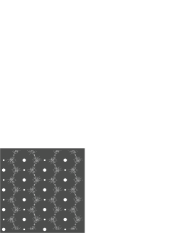
Figure 4: Typical tiling for $\rho_{2}=0.24$ and $\rho_{1}=\rho_{3}=0.38$ (left) and its diffraction image (right). The scatterers are located at the centres of the tiles.

As before, we will now show that the remaining part of $\hat{\gamma}_{\omega}$ converges to a periodic $L^{1}$-function and thus represents an absolutely continuous measure. Let us start with the case $x\leq-1$ (and $y$ arbitrary, but fixed) and show that $[x,y|z_{1},z_{2},z_{3}]_{LR}=\mathcal{O}\left({|x|^{-1}}\right)$ as $x\to-\infty$. The necessary extension to the complete asymptotic behaviour will later follow from Eq. (89). For now, and for fixed values of the activities in the admitted range, we have

$$I\;=\;\left|\,[x,y|z_{1},z_{2},z_{3}]_{LR}\,\right| \;\leq\;\frac{z_{1}^{x}}{2\pi}\int_{e^{i\varphi_{0}}}^{e^{i(2\pi-\varphi_{0})}}|z_{2}+z_{3}w|^{-x-1}|dw|$$

$$\;=\;\frac{z_{1}^{x}}{\pi}\int_{\varphi_{0}}^{\pi}\left(z_{2}^{2}+z_{3}^{2}+2z_{2}z_{3}\cos\vartheta\right)^{\frac{-x-1}{2}}d\vartheta.$$ (93)

We first bound $f(\vartheta)=(z_{2}^{2}+z_{3}^{2}+2z_{2}z_{3}\cos\vartheta)/z_{1}^{2}$ by a straight line $\tilde{f}(\vartheta)$, i.e. we look for $f(\vartheta)\leq\tilde{f}(\vartheta)$ on the interval $[\varphi_{0},\pi]$. Note that $f(\vartheta)$ can only have one flex point at $\vartheta=\pi/2$ in $[0,\pi]$. One has to distinguish two cases:

1. $\cos\varphi_{0}\geq(\pi-\varphi_{0})\sin\varphi_{0}-1$: Choose $\tilde{f}_{1}(\vartheta)=(\vartheta-\varphi_{0})f^{\prime}(\varphi_{0})+f(\varphi_{0})$. The condition on $\varphi_{0}$ implies $\tilde{f}_{1}(\pi)\geq f(\pi)$. Differentiating $f(\vartheta)-\tilde{f}_{1}(\vartheta)$ with respect to $\vartheta$ yields $f^{\prime}(\vartheta)-\tilde{f}_{1}^{\prime}(\vartheta)=f^{\prime}(\vartheta)-f^{\prime}(\varphi_{0})$ and this vanishes if $\vartheta=\varphi_{0}$ (maximum) or if $\vartheta=\pi-\varphi_{0}$ (minimum). Thus $f(\vartheta)\leq\tilde{f}_{1}(\vartheta)$.

2. $\cos\varphi_{0}<(\pi-\varphi_{0})\sin\varphi_{0}-1$: Choose $\tilde{f}_{2}(\vartheta)=\frac{f(\pi)-1}{\pi-\varphi_{0}}\vartheta+\frac{\pi-\varphi_{0}f(\pi)}{\pi-\varphi_{0}}$ (the line connecting $f(\varphi_{0})=1$ and $f(\pi)$). Obviously $\tilde{f}^{\prime}_{2}(\pi)\leq f^{\prime}(\pi)$. Because of the angle condition, we further have $f^{\prime}(\varphi_{0})\leq\tilde{f}^{\prime}_{2}(\varphi_{0})$. As there is only one flex point, we conclude that $f(\vartheta)\leq\tilde{f}_{2}(\vartheta)$.

Choose $f(\vartheta)$ as $f_{1}(\vartheta)$ or $f_{2}(\vartheta)$ according to the previous distinction. If $c=|\tilde{f}^{\prime}(\vartheta)|$, we get $0<c\leq\frac{1}{\pi-\varphi_{0}}\left(1-\frac{(z_{2}-z_{3})^{2}}{z_{1}^{2}}\right)<\frac{1}{\pi-\varphi_{0}}$. Consequently, we can estimate

$$\pi z_{1}I \;\leq\;\int_{\varphi_{0}}^{\pi}\left(1-c(\vartheta-\varphi_{0})\right)^{\frac{-x-1}{2}}d\vartheta$$

$$\;<\;\frac{1}{c}\int_{0}^{1}(1-t)^{\frac{-x-1}{2}}\,dt$$ (94)

$$\;=\;\frac{2}{c(1-x)}\;=\;\mathcal{O}\left(\frac{1}{|x|}\right).$$

Now, we can use the symmetry relations of (89) and obtain the asymptotic behaviour $[x,y|z_{1},z_{2},z_{3}]_{LR}=\mathcal{O}\left({(|x|+|y|)^{-1}}\right)$, whenever $|\boldsymbol{r}|\to\infty$, compare [37]. The rest of the argument is very similar to the domino case and need not be repeated here, the periodicity statement follows again constructively. $\square$

Let us remark that an analogous scenario, with the same type of result, occurs for the more complicated dart-rhombus random tiling, see [25] for details.

Addendum: The two-dimensional Ising model

For the sake of completeness, we add an application of the probably best analyzed model in statistical physics, the 2D Ising model without external field. It may be regarded as a lattice gas on $\mathbb{Z}^{2}$, compare [55], with scatterers of strength $s_{(i,j)}\in\{1,0\}$. The partition function in the spin-formulation ($\sigma_{(i,j)}\in\{+1,-1\}$) reads as follows

$$\mathcal{Z}\;=\;\sum_{\{\boldsymbol{\sigma}\}}\exp\left(\sum_{(i,j)}\sigma_{(i,j)}\left(K_{1}\sigma_{(i+1,j)}+K_{2}\sigma_{(i,j+1)}\right)\right)\,,$$ (95)

where we sum over all configurations $\{\boldsymbol{\sigma}\}$. We consider the ferromagnetic case with coupling constants $K_{i}=J_{i}/(k_{B}T)>0$, temperature $T$ and Boltzmann’s constant $k_{B}$. The model undergoes a phase transition at $k:=\left(\sinh(2K_{1})\sinh(2K_{2})\right)^{-1}=1$. It is common knowledge that in the regime with coupling constants smaller than the critical ones (corresponding to $T>T_{c}$) the ergodic equilibrium state with vanishing magnetization $m$ is unique, whereas above ($T<T_{c}$) there exist two extremal equilibrium states, which are thus ergodic [55, Ch. III.5]. In this case, we assume to be in the extremal state with positive magnetization $m=(1-k^{2})^{1/8}$.

The diffraction properties of the Ising model can be extracted from the known asymptotic behaviour [42, 59] of the autocorrelation coefficients. We first state the result for the isotropic case ($K_{1}=K_{2}=K$) and comment on the general case later.

Proposition 5

Away from the critical point, the diffraction spectrum of the Ising lattice gas almost surely exists, is $\mathbb{Z}^{2}$-periodic and consists of a pure point and an absolutely continuous part with continuous density. The pure point part reads

1. $T>T_{c}$: $(\hat{\gamma}_{\omega})_{pp}=\frac{1}{4}\sum_{\boldsymbol{k}\in\mathbb{Z}^{2}}\delta_{\boldsymbol{k}}$

2. $T<T_{c}$: $(\hat{\gamma}_{\omega})_{pp}=\rho^{2}\sum_{\boldsymbol{k}\in\mathbb{Z}^{2}}\delta_{\boldsymbol{k}}$,

where the density $\rho$ is the ensemble average of the number of scatterers per unit volume.

Proof: First, note that $s_{(i,j)}=(\sigma_{(i,j)}+1)/2$ and thus $\langle\sigma_{(i,j)}\rangle=m=2\rho-1$, so $\rho$ varies between $1$ and $1/2$. The asymptotic correlation function of two spins at distance $R=\sqrt{x^{2}+y^{2}}\,$ (as $R\to\infty$) is [42]

$$\langle\sigma_{(0,0)}\sigma_{(x,y)}\rangle\;\simeq\;\begin{cases}c_{1}\frac{e^{-R/c_{2}}}{\sqrt{R}},&T>T_{c}\\ m^{2}+c_{3}\frac{e^{-2R/c_{2}}}{R^{2}},\quad&T<T_{c},\end{cases}$$ (96)

with constants $c_{1},c_{2}$ and $c_{3}$ depending only on $K$ and $T$, see also [39, p. 51] and references given there for a summary. The pure point part $(\hat{\gamma}_{\omega})_{pp}$ results directly from the Fourier transform of the constant part of $\gamma_{\omega}$ as derived from the asymptotics of $\langle s_{(0,0)}s_{(x,y)}\rangle=(\langle\sigma_{(0,0)}\sigma_{(x,y)}\rangle+2m+1)/4$.

Here, already $\sum_{(x,y)\in\mathbb{Z}^{2}}e^{-R/c_{2}}/\sqrt{R}$ and $\sum_{(x,y)\in\mathbb{Z}^{2}}e^{-2R/c_{2}}/R^{2}$ converge absolutely, so we can view the corresponding correlation coefficients as functions in $L^{1}(\mathbb{Z}^{2})$. Their Fourier transforms (which are uniformly converging Fourier series) are continuous functions on $\mathbb{R}^{2}/\mathbb{Z}^{2}$, see [48, §1.2.3], which are then also in $L^{1}(\mathbb{R}^{2}/\mathbb{Z}^{2})$. Applying the Radon-Nikodym theorem finishes the proof. $\square$

Remark: At the critical point, the correlation function $\langle\sigma_{(0,0)}\sigma_{(x,y)}\rangle$ is asymptotically proportional to $R^{-1/4}$ as $R\to\infty$ [59, 39]. Again, taking out first the constant part of $\gamma_{\omega}$, we get the same pure point part as in Prop. 5 for $T>T_{c}$. However, for the remaining part of $\gamma_{\omega}$, both our previous arguments fail. Nevertheless, using a theorem of Hardy [9, p. 97], we can show that the corresponding Fourier series still converges for $\boldsymbol{k}\not\in\mathbb{Z}^{2}$ (a natural order of summation is given by shells of increasing radius).

For $\boldsymbol{k}\in\mathbb{Z}^{2}$, where the Bragg peaks reside, the series diverges. But this can neither result in further contributions to the Bragg peaks (the constant part of $\gamma_{\omega}$ had already been taken care of) nor in singular continuous contributions (because the points of divergence form a uniformly discrete set). So, even though the series diverges for $\boldsymbol{k}\in\mathbb{Z}^{2}$, it still represents (we know that $\hat{\gamma}_{\omega}$ exists) a function in $L^{1}(\mathbb{R}^{2}/\mathbb{Z}^{2})$ and hence the Radon-Nikodym density of an absolutely continuous background. On the diffraction image, we thus can see, for any temperature, Bragg peaks on the square lattice and a $\mathbb{Z}^{2}$-periodic, absolutely continuous background concentrated around the peaks (the interaction is attractive). At the critical point, the intensity of the diffuse scattering diverges when approaching the lattice positions of the Bragg peaks.

The same arguments hold in the anisotropic case, where the asymptotics still conforms to Eq. (96) and the above, if $R=R(x,y)$ is replaced by the formula given in [59, Eq. 2.6]. The pure point part is again that of Prop. 5 with fourfold symmetry, while (as in the case of the domino tiling) the continuous background breaks this symmetry if $K_{1}\neq K_{2}$. Let us finally remark that a different choice of the scattering strengths (i.e. $\pm 1$ rather than $1$ and $0$) would result in the extinction of the Bragg peaks in the disordered phase ($T>T_{c}$), but no choice does so in the ordered phase ($T<T_{c}$).

Outlook

The diffraction of crystallographic and of perfect quasi-crystallographic structures is well understood. The main aim of this article was to begin to counterbalance this into the direction of certain stochastic arrangements of scatterers, and to random tiling arrangements in particular. This requires a careful investigation of the diffuse background and clear concepts about absolutely versus singular continuous contributions. Such problems are naturally studied via spectral properties of unbounded complex measures which we did for a number of simple, but relevant examples.

While stochastic cuboid tilings would generically display a singular continuous contribution in the diffraction image, our results on the domino and the lozenge tilings show that no such contributions exist there. However, we do not think that this is a robust result. In fact, the natural next step would be an extension to planar random tilings with quasi-crystallographic symmetries such as 8-, 10- or 12-fold. Then, according to the folklore results, one should expect a purely continuous diffraction spectrum (except for the trivial Bragg peak at $\boldsymbol{k}=0$ which merely reflects the existing natural density of the scatterers). This spectrum should then split into an $ac$ and an $sc$ part.

But is the replacement of Bragg peaks by $sc$ peaks significant? Scaling arguments [23] and numerical calculations [33] indicate that the exponents of important $sc$ peaks can be extremely close to $1$ which means that their distinction from Bragg peaks is almost impossible in practice. Is it possible that this is one reason why structure refinement is so difficult for real decagonal quasicrystals? This certainly demands further thought, but it is not clear at the moment to what extent a rigorous treatment is possible.

Finally, except for Bernoulli type systems [4] and for extensions by means of products of measures, we have not touched the “real” diffraction issues in 3-space. One reason is that we presently do not know of any interesting model that can be solved exactly (let alone rigorously), another is that, for random tiling models relevant to real quasicrystals, one expects bounded fluctuations (again, due to heuristic scaling arguments, see [23] and references therein). Consequently, the diffraction spectra should typically show Bragg peaks plus an absolutely continuous background. We hope to report on some progress soon.

References

- [1] L. Argabright and J. Gil de Lamadrid, Fourier Analysis of Unbounded Measures on Locally Compact Abelian Groups, Memoirs of the AMS, vol. 145, AMS, Providence, RI (1974).
- [2] J. Arsac, Fourier Transforms and the Theory of Distributions, Prentice Hall, Englewood Cliffs (1966).
- [3] M. Baake, “A guide to mathematical quasicrystals”, in: Quasicrystals, eds. J.-B. Suck, M. Schreiber and P. Häußler, Springer, Berlin (2001), in press; math-ph/9901014.
- [4] M. Baake and R. V. Moody, “Diffractive point sets with entropy”, J. Phys. A31 (1998) 9023–39; math-ph/9809002.
- [5] M. Baake, R. V. Moody and P. A. B. Pleasants, “Diffraction from visible lattice points and th power free integers”, Discr. Math. 221 (2000) 3–42; math.MG/9906132.
- [6] M. Baake, R. V. Moody and M. Schlottmann, “Limit-(quasi-)periodic point sets as quasicrystals with -adic internal spaces” J. Phys. A31 (1998) 5755–65.
- [7] H. Bauer, Maß- und Integrationstheorie, 2nd ed., de Gruyter, Berlin (1992).
- [8] S. K. Berberian, Measure and Integration, Macmillan, New York (1965).
- [9] T. J. I’A. Bromwich, An Introduction to the Theory of Infinite Series, 2nd rev. ed., Macmillan, London (1965); reprint, Chelsea, New York (1991).
- [10] R. Burton and R. Pemantle, “Local characteristics, entropy and limit theorems for spanning trees and domino tilings via transfer-impedances”, Ann. Prob. 21 (1993) 1329–71.
- [11] J. W. S. Cassels, An Introduction to Diophantine Approximation, Cambridge University Press, Cambridge (1957).
- [12] J. M. Cowley, Diffraction Physics, 3rd ed., North-Holland, Amsterdam (1995).
- [13] L. Danzer, “A family of 3D-spacefillers not permitting any periodic or quasiperiodic tiling”, in: Aperiodic ’94, eds. G. Chapuis and W. Paciorek, World Scientific, Singapore (1995), pp. 11–7.
- [14] J. Dieudonné, Treatise of Analysis, vol. II, Academic Press, New York (1970).
- [15] S. Dworkin, “Spectral theory and -ray diffraction”, J. Math. Phys. 34 (1993) 2965–7.
- [16] V. Elser, “Comment on: Quasicrystals – A New Class of Ordered Structures”, Phys. Rev. Lett. 54 (1985) 1730.
- [17] W. Feller, An Introduction to Probability Theory and its Applications; vol. 1, 3rd ed., rev. printing, Wiley, New York (1970); vol. 2, 2nd ed., Wiley, New York (1991).
- [18] M. E. Fisher and J. Stephenson, “Statistical mechanics of dimers on a plane lattice. II. Dimer correlations and monomers”, Phys. Rev. 132 (1963) 1411–31.
- [19] H.-O. Georgii, Gibbs Measures and Phase Transitions, de Gruyter, Berlin (1988).
- [20] A. Guinier, -ray Diffraction in Crystals, Imperfect Crystals and Amorphous Bodies, Freeman, San Francisco (1963); reprinted as Dover, New York (1994).
- [21] E. R. Hansen, A table of series and products, Prentice Hall, Englewood Cliffs (1975).
- [22] O. J. Heilmann and E. H. Lieb, “Lattice models for liquid crystals”, J. Stat. Phys. 20 679–93.
- [23] C. L. Henley, “Random tiling models”, in: Quasicrystals - The State of the Art, eds. D. P. DiVincenzo and P. J. Steinhardt, World Scientific, Singapore (1991), pp. 429–524; 2nd ed. in preparation.
- [24] H. Heuser, Funktionalanalysis, 2nd ed., Teubner, Stuttgart (1986).
- [25] M. Höffe, “Diffraction of the dart-rhombus random tiling”, to appear in: Mat. Science Eng. A, in press; math-ph/9911014.
- [26] A. Hof, “On diffraction by aperiodic structures”, Commun. Math. Phys. 169 (1995) 25–43.
- [27] A. Hof, “Diffraction by aperiodic structures”, in: The Mathematics of Long-Range Aperiodic Order, ed. R. V. Moody, NATO ASI Series C 489, Kluwer, Dordrecht (1997), pp. 239–68.
- [28] A. Hof, “Diffraction by aperiodic structures at high temperatures”, J. Phys. A28 (1995) 57–62.
- [29] A. Hof, “On scaling in relation to singular spectra”, Commun. Math. Phys. 184 (1997) 567–77.
- [30] R. B. Israel, Convexity in the Theory of Lattice Gases, Princeton University Press, Princeton (1979).
- [31] H. Jagodzinski and F. Frey, “Disorder diffuse scattering of -rays and neutrons”, in: International Tables of Crystallography B, ed. U. Shmueli, 2nd ed., Kluwer, Dordrecht (1996), pp. 392–433.
- [32] M. V. Jarić and D. R. Nelson, “Diffuse scattering from quasicrystals”, Phys. Rev. B37 (1988) 4458–72.
- [33] D. Joseph, private communication (1998).
- [34] P. W. Kasteleyn, “The statistics of dimers on a lattice”, Physica 27 (1961) 1209–25.
- [35] P. W. Kasteleyn, “Dimer statistics and phase transitions”, J. Math. Phys. 4 (1963) 287–93.
- [36] G. Keller, Equilibrium States in Ergodic Theory, LMSST 42, Cambridge University Press, Cambridge (1998).
- [37] R. Kenyon, “Local statistics of lattice dimers”, Ann. Inst. H. Poincaré Prob. 33 (1997) 591–618.
- [38] R. Kenyon, “The planar dimer model with boundary: a survey”, preprint (1998); in: Directions in Mathematical Quasicrystals, eds. M. Baake and R. V. Moody, CRM Monograph Series, AMS, Providence, RI (2000), in press.
- [39] R. Kindermann and J. L. Snell, Markov Random Fields and their Applications, Contemp. Mathematics, vol. 1, AMS, Providence, RI (1980).
- [40] J. C. Lagarias and P. A. B. Pleasants, “Repetitive Delone sets and quasicrystals”, to appear in: Erg. Th. & Dyn. Syst.; math.DS/9909033.
- [41] W. Ledermann, “Asymptotic formulae relating to the physical theory of crystals”, Proc. Royal Soc. London A182 (1943-44) 362–77.
- [42] B. M. McCoy and T. T. Wu, The Two-Dimensional Ising Model, Harvard University Press, Cambridge, MA (1973).
- [43] E. W. Montroll, “Lattice Statistics”, in: Applied Combinatorial Mathematics, ed. E. F. Beckenbach, John Wiley, New York (1964), pp. 96–143.
- [44] K. Petersen, Ergodic Theory, Cambridge University Press, Cambridge (1983).
- [45] M. Queffélec, “Spectral study of automatic and substitutive sequences”, in: Beyond Quasicrystals, eds. F. Axel and D. Gratias, Springer, Berlin (1995), pp. 369–414.
- [46] M. Reed and B. Simon, Methods of Modern Mathematical Physics I: Functional Analysis, 2nd ed., Academic Press, San Diego (1980).
- [47] C. Richard, M. Höffe, J. Hermisson and M. Baake, “Random tilings – concepts and examples”, J. Phys. A31 (1998) 6385–408.
- [48] W. Rudin, Fourier Analysis on Groups, Wiley Interscience, New York (1962).
- [49] W. Rudin, Functional Analysis, 2nd ed., McGraw-Hill, New York (1991).
- [50] D. Ruelle, Statistical Mechanics: Rigorous Results, Addison Wesley, Redwood City (1969).
- [51] D. Ruelle, “Do turbulent crystals exist?”, Physica 113 A (1982) 619–23.
- [52] M. Schlottmann, “Cut-and-project sets in locally compact Abelian groups”, in: Quasicrystals and Discrete Geometry, ed. J. Patera, Fields Institute Monographs, vol. 10, AMS, Providence, RI (1998), pp. 247–64.
- [53] M. Schlottmann, “Generalized model sets and dynamical systems”, in: Directions in Mathematical Quasicrystals, eds. M. Baake and R. V. Moody, CRM Monograph Series, AMS, Providence, RI (2000), in press.
- [54] L. Schwartz, Théorie des Distributions, 3rd ed., Hermann, Paris (1998).
- [55] B. Simon, The Statistical Mechanics of Lattice Gases, Vol. 1, Princeton University Press, Princeton (1993).
- [56] C. J. Thompson, Mathematical Statistical Mechanics, Princeton University Press, Princeton (1972).
- [57] A. C. D. van Enter and J. Miȩkisz, “How should one define a (weak) crystal?”, J. Stat. Phys. 66 (1992) 1147–53.
- [58] T. R. Welberry, “Diffuse -ray scattering and models of disorder”, Rep. Prog. Phys. 48 (1985) 1543–93.
- [59] T. T. Wu, B. M. McCoy, C. A. Tracy and E. Barouch, “Spin-spin correlation functions for the two-dimensional Ising model: Exact theory in the scaling region”, Phys. Rev. B13 (1976) 316–74.
- [60] R. Youngblood, J. D. Axe and B. M. McCoy, “Correlations in ice-rule ferroelectrics”, Phys. Rev. B21 (1980) 5212–20.