The Rotor Model with spectral parameters and enumerations of Alternating Sign Matrices.

Luigi Cantini

In this paper we study the Rotor Model of Martins and Nienhuis. After introducing spectral parameters, a combined use of integrability, polynomiality of the ground state wave function and a mapping into the fully-packed $O(1)$-model allows us to determine the sum rule and a family of maximally nested components for different boundary conditions. We see in this way the appearance of 3-enumerations of Alternating Sign Matrices.

1 Introduction

In recent years it has become clear that some exactly integrable models present a deep and somehow unexpected combinatorial structure, related to various enumerations of alternating sign matrices (ASM). Such matrices appeared for the first time in the work of Mills, Robbins and Rumsey [1], and from that moment on they have played a fundamental role in modern developments of combinatorics [2]. An ASM is a matrix with only $0,1,-1$ entries, such that on each row and on each column $1$s and $-1$s appear alternately, possibly separated by zeroes and the sum on each row and each column is equal to $1$.

In a series of remarkable papers [3] Razumov and Stroganov noticed the appearance of various enumerations of ASMs in the components of the ground state of the XXZ spin chain at $\Delta=-1/2$. After [3] many other models with different boundary conditions have been object of investigation, leading to a plethora of conjectures (for a review see [4]).

A first step towards the proof of these conjectures was made by Di Francesco and Zinn-Justin in [7]. Their idea, first applied to the fully packed $O(1)$ loop-model [5, 6], was to introduce spectral parameters, so that the components of the ground state become polynomials in these. Then, making use of the integrability of the model, they were able to prove a set of equations satisfied by these polynomials, which were generalised and reinterpreted as qKZ equations [8, 9]. In that way they were not only able to prove a conjecture related to the sum rule, but they also discovered the deep role of algebraic geometry in the game [10].

In the present article we apply the idea of Di Francesco and Zinn-Justin to the study of a model introduced by Martins and Nienhuis [11] and called rotor model. In [12] Batchelor, de Gier and Nienhuis have computed numerically the components of the ground state of the rotor model for different boundary conditions. It turned out that these components could be normalised in such a way that they are all positive integers. Moreover, taking the greater common divisor equal to $1$, their sum was given by an enumeration of certain classes of ASMs with extra symmetry.

Motivated by these results, we study the rotor model with spectral parameters. As usual the value of the degree of the minimal polynomial solution is quite hard to derive. Here we make the assumption, justified by the explicit solutions for small sizes and a posteriori by the evaluation at the homogeneous point, that the degree is two times the degree of the corresponding fully packed $O(1)$ model.

Then we find on one hand that the polynomial sum rules are quite easy to derive, using a mapping to the $O(1)$ model. On the other hand contrarily to the $O(1)$ model, where the smallest component is given by a product of degree-one terms, for the rotor model there are no completely factorized components. Nonetheless we are able to compute explicitly a whole family of terms which we call maximally nested components and which in most cases contains the smallest component. We see in this context the appearance of $3-$enumerations of alternating sign matrices.

The plan of the article is as follows: in Sect. 2 we give a brief description of the rotor model with different boundary conditions. In Sect. 3 we introduce the spectral parameters. We find a mapping of our model to the fully packed $O$(1) model, which will allow us to derive most of the recursion relations we need. We write also the exchange equation. Then in Sect. 4 we come to the main results of our paper: the sum rules and the maximally nested components for periodic and open boundary conditions.

2 The rotor model

The rotor model [11, 12] is defined on a square lattice. In the interior of a face there are four lines that can be thought as the paths followed by four cars coming from different directions at a crossroad, under the condition that each car turns right or left and no two cars go in the same direction. Under this restriction there are only the four possible configurations for a face called $R,L,A,D$. Each configuration appears with probability respectively $\omega_{R},\omega_{L},\omega_{A},\omega_{D}$.

Configurations.

Once all the faces of the lattice are assigned, one gets a global configuration consisting of closed loops and, in presence of boundaries, open curves connecting points on the boundary. We are interested in geometries where the lattice is semi-infinite in one direction (the vertical one) and finite in the other. Let us label the rows ascending from 1 to $\infty$ and the columns from left to right in such a way that each face is labelled by a pair $(i,j)$. Now, depending on the parity of $i+j$, let us colour the lines of our configurations in red and green in the following way

Coloration for $i+j$ even.

Coloration for $i+j$ odd.

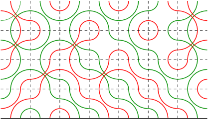
Figure 1: An example of the result of the coloration on a sample configuration

As one can see from fig. 1 red (green) lines join only red (green) lines and lines of different colours can cross (inside a $D$ face), while lines of the same colour cannot. The points on the boundary can be connected only if they have the same colour, and looking at each colour separately we will have a link pattern of non-crossing lines like in the fully packed $O(1)$ case. For example, the connectivities of fig. 1 give the link pattern of fig. 2

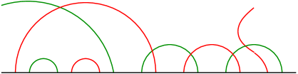
Figure 2: Link pattern corresponding to the sample of fig. 1

In the horizontal direction we always choose boundary conditions which respect the colouration. They can be periodic (PBC) or closed (CBC). The periodic boundary conditions for lattice of even size of course preserve the coloration. In the case of a lattice of odd size we have to introduce a vertical seam that exchanges the colours in the horizontal direction. We are interested in the connectivities, hence each configuration corresponds to a pair of non-intersecting link patterns (red and green) which for the periodic lattice can be draw a disk. Actually for even period lattices we could also take trace of the presence of the hole in the cylinder, in this case we call the boundary conditions PBC+$\infty$ and each configuration is mapped to two link patterns on a punctured disk.

The closed boundary conditions are defined in the following way: take the four points on the right boundary of a pair of rows $2i-1,2i$ and connect them in a way consistent with the colouration (do the same on the left). Here the connectivities can be drawn on the upper-half plane.

Closed boundary conditions.

We are interested in the probability of having a certain connectivity of the base points or, in the light of what we have said above, of having a pair of link patterns $(\pi_{G},\pi_{R})$.

The standard technique to deal with this kind of problems makes use of the transfer matrix $T$, whose effect is that of adding one (or two for CBC) more rows to the cylinder. The link patterns probability has to be stationary under this action. This simply means that it forms an eigenvector of $T$ with eigenvalue 1.

Having given the general setting, we restrict our attention to the choice of the weights that gives an integrable system. Let us introduce the $R-$matrix

in terms of which the one-row transfer matrix for periodic lattices reads

For CBC the double-row transfer matrix is given in terms of the $R-$matrix introduced above and the boundary $K-$matrix, which in our case has the simple effect of inverting the spectral parameter

In [11] Martins and Nienhius have solved the Yang-Baxter equation for the previous R-matrix, finding three classes of solutions. Here, following [12], we consider only what in [11] is called class II

$$\omega_{R}(z,w)=\omega_{L}(z,w)\leavevmode\nobreak\ =\leavevmode\nobreak\ (w-z)(z+qw);$$ (1)

$$\omega_{D}(z,w)\leavevmode\nobreak\ =\leavevmode\nobreak\ q(w-qz)(z+qw)$$ (2)

$$\omega_{A}(z,w)\leavevmode\nobreak\ =\leavevmode\nobreak\ (w-z)(w+qz)$$ (3)

where $q=e^{2\pi i/3}$ and $z,w$ are spectral parameters.

Notice that we have not normalised the sum of the $\omega_{i}$ to be $1$, but $\omega_{R}+\omega_{L}+\omega_{A}+\omega_{D}=qz^{2}-w^{2}$

What Batchelor et al. have done in [12] is to compute the probabilities of link-patterns for different boundary conditions and different lattice size. In terms of the eigenvector of the transfer matrix they have found that one can choose a normalisation such that all the components are integers and the GCD equals 1. In particular they were able to identify the sum $S$ of the components and in case of a odd size lattice with CBC the smallest component:

• PBC - Even: $S(2n)=3^{\theta_{n}}A(n;1)$;

• PBC - Odd: $S(2n+1)=3^{3n}A_{V}(2n-1;3)^{2}$;

• PBC+$\infty$ -: $S(2n)=3^{n^{2}}A_{HT}(2n)$;

• CBC - Even: $S(2n)=3^{2\theta_{n}}A_{V}(2n+1)$;

• CBC - Odd: $S(2n-1)=3^{(n-1)^{2}}\mathscr{N}_{8}(2n)$;

where $\theta_{n}=\lfloor(n-1)(n+2)/3\rfloor$ and the other quantities will be defined in the following.

In the present paper we not only prove these conjectures but we also determine the value of a family of components having maximally nested arcs. This family, in all cases except for CBC and even size, contains the smallest component.

In the case of lattices of size $2n$ with PBC, each MNC is given by the product of two 3-enumerations of ASMs $A(m;3)A(k;3)$, where $m$ and $k$ represent the relative orientation of the red and green link patterns. The smallest component is then given by $A(\lfloor n/2\rfloor;3)A(\lfloor(n+1)/2\rfloor;3)$.

For periodic systems in which we keep track of the hole in the cylinder we give a Pfaffian formula for the values of the MNCs, but we have not been able to recognise these numbers as enumerations of some known objects.

In the case of closed boundary conditions, we have computed the smallest component for odd size, and found $A_{V}(2n+1;3)$ (this in fact is the only value predicted in [12]). For lattices of even size we have computed the MNC with all arcs parallel (which is not the smallest one), and found again $A_{V}(2n+1;3)$.

3 Spectral parameters

Up to now the probabilities $\omega_{R},\omega_{L},\omega_{A},\omega_{D}$ were independent of the face position. The key idea of Di Francesco and Zinn-Justin [7] was to generalise the problem considering different spectral parameters $z_{i}$ for each vertical line. In the following we will explicitly treat the case of PBC and even size lattice, the other cases being completely analogous. At the proper moment we will point out the differences.

In presence of spectral parameters the transfer matrix $T(t|z_{1},\dots,z_{2n})$ becomes

$$T(t|z_{1},\dots,z_{2n})={\rm Tr}R(z_{1},t)R(z_{2},t)\dots R(z_{2n},t)$$ (4)

Because of the normalisation, the eigenvector equation we have to study assumes the form

$$T(t|z_{1},\dots,z_{2n})\Psi(z_{1},\dots,z_{2n})=\prod_{i=1}^{2n}(qz_{i}^{2}-t^{2})\leavevmode\nobreak\ \Psi(z_{1},\dots,z_{2n})$$ (5)

Introducing a basis of of pairs of link patterns (red and green) $|\pi_{R}\rangle\otimes|\pi_{G}\rangle$, we write

$$\Psi(z_{1},\dots,z_{2n})=\sum_{\pi_{R},\pi_{G}}\Psi_{\pi_{R},\pi_{G}}(z_{1},\dots,z_{2n})|\pi_{R}\rangle\otimes|\pi_{G}\rangle$$ (6)

where, if we normalise the sum to be $1$, $\Psi_{\pi_{R},\pi_{G}}(z_{1},\dots,z_{2n})$ is the probability of having the link pattern configuration $\pi_{R},\pi_{G}$.

A couple of remarks are in order.

• The fact that $\Psi$ doesn’t depend on $t$ is a trivial consequence of the commutativity of the transfer matrices for different values of the parameter $t$.

  $$[T(t|z_{1},\dots,z_{2n}),T(t^{\prime}|z_{1},\dots,z_{2n})]=0.$$

• It is easy to see that the transpose of the transfer matrix has a very simple eigenvector of eigenvalue $\Lambda=\prod_{i=1}^{2n}(qz_{i}^{2}-t^{2})$, namely

  $$\langle\Omega|:=\left(\sum_{\pi_{R}}\langle\pi_{R}|\right)\otimes\left(\sum_{\pi_{G}}\langle\pi_{G}|\right).$$ (7)

  It is simply the functional which gives 1 on each link configuration.

• The solution of eq.(4) can be normalised to be a homogeneous polynomial. We require it to be of minimum degree.

Let us introduce the matrix $\check{R}$

$$\check{R}_{i}(z,w)=q(w-qz)(qw+z){\rm Id}+(w-z)(w+qz)E_{i}+(w-z)(qw+z)(R_{i}+L_{i})$$ (8)

The operators $E_{i},R_{i},L_{i}$ for $i=1,\dots,N$ satisfy the following relations

$$\begin{split}&E_{i}=R_{i}L_{i}=L_{i}R_{i},\leavevmode\nobreak\ \leavevmode\nobreak\ \leavevmode\nobreak\ \leavevmode\nobreak\ \leavevmode\nobreak\ \leavevmode\nobreak\ R_{i}^{2}=R_{i}\leavevmode\nobreak\ \leavevmode\nobreak\ \leavevmode\nobreak\ \leavevmode\nobreak\ \leavevmode\nobreak\ \leavevmode\nobreak\ L_{i}^{2}=L_{i}\\ &L_{i}R_{i\pm 1}L_{i}=L_{i},\leavevmode\nobreak\ \leavevmode\nobreak\ \leavevmode\nobreak\ \leavevmode\nobreak\ \leavevmode\nobreak\ \leavevmode\nobreak\ R_{i}L_{i\pm 1}R_{i}=L_{i},\leavevmode\nobreak\ \leavevmode\nobreak\ \leavevmode\nobreak\ \leavevmode\nobreak\ \leavevmode\nobreak\ \leavevmode\nobreak\ [R_{i},R_{i\pm 1}]=[L_{i},L_{i\pm 1}]=0\\ &[R_{i},R_{j}]=[L_{i},L_{j}]=[R_{i},L_{j}]=0\leavevmode\nobreak\ \leavevmode\nobreak\ \leavevmode\nobreak\ \leavevmode\nobreak\ |i-j|\geq 2\end{split}$$ (9)

and have the following graphical representation

The $R-$matrix/$\check{R}-$matrix and the $K-$matrix, besides the Yang-Baxter and the boundary Yang-Baxter equation, satisfy the unitarity property

and the inversion relation

3.1 Mapping to the $O(1)$ model

As described above, the vector space of configurations of the rotor model can be seen as a tensor product of two copies of the vector space of the $O(1)$ model. Tracing on one of the two colours (say tracing on green) is equivalent to mapping the rotor model on the $O(1)$ model. It is very easy to realise the effect of the trace $\mathscr{T}=\sum\langle\pi_{G}|$ on the transfer matrix or on the $\check{R}$ matrix

$$\mathscr{T}T(t|z_{1},\dots,z_{2n})=T_{O(1)}(t^{2}|z_{1}^{2},\dots,z_{2n}^{2})\mathscr{T},\leavevmode\nobreak\ \leavevmode\nobreak\ \leavevmode\nobreak\ \leavevmode\nobreak\ \leavevmode\nobreak\ \leavevmode\nobreak\ \mathscr{T}\check{R}(z_{i},z_{j})=\check{R}_{O(1)}(z_{i}^{2},z_{j}^{2})\mathscr{T}.$$ (10)

In particular this means that for the eigenvectors is valid the following

$$\mathscr{T}\Psi(z_{1},\dots,z_{2n})\propto\Psi_{O(1)}(z_{1}^{2},\dots,z_{2n}^{2}).$$ (11)

In this paper we make the assumption that the degree of $\Psi$ in each variable is two times the degree of $\Psi_{O(1)}$. Hence we can choose the normalisation of $\Psi$ in such a way that the proportionality in eq.(11) becomes an equality.

3.2 Exchange equations

As a consequence of the Yang-Baxter equation we have the following

Proposition 1

The transfer matrices $T(t;\dots,z_{i},z_{i+1},\dots)$ and $T(t;\dots,z_{i+1},z_{i},\dots)$ are intertwined by $\check{R}_{i,i+1}(z_{i},z_{i+1})$, i.e.

$$T(t;..,z_{i},z_{i+1},..)\check{R}_{i,i+1}(z_{i},z_{i+1})=\check{R}_{i,i+1}(z_{i},z_{i+1})T(t;..,z_{i+1},z_{i},..).$$ (12)

From proposition (1) it follows

$$\check{R}_{i,i+1}(z_{i},z_{i+1})\Psi(..,z_{i+1},z_{i},..)=\alpha_{i}(z_{1},..,z_{i},z_{i+1},..,z_{2n})\Psi(..,z_{i},z_{i+1},..)$$ (13)

where $\alpha_{i}$ is a polynomial which can be determined using the projection to the $O(1)$ model

$$\alpha_{i}(..,z_{i},z_{i+1},..)=\alpha(z_{i},z_{i+1})=(qz_{i+1}^{2}-z_{i}^{2}).$$

Alternatively, for even PBC one can derive $\alpha_{i}$ without making use of the projection. From the unitarity condition it follows

$$\alpha_{i}(z_{1},..,z_{i},z_{i+1},..,z_{2n})\alpha_{i}(z_{1},..,z_{i+1},z_{i},..,z_{2n})=q^{2}(z_{i}^{2}-q^{2}z_{i+1}^{2})(z_{i+1}^{2}-q^{2}z^{2}_{i}),$$ (14)

then we notice that the left eigenvalue defined in eq.(7) satisfies

$$\langle\Omega|\check{R}_{i,i+1}(z_{i},z_{i+1})=q(z_{i+1}+qz_{i})(z_{i+1}-qz_{i})\langle\Omega|$$ (15)

Hence

$$\begin{split}\prod_{i=1}^{2n-1}(qz_{2n}^{2}-z_{i}^{2})\leavevmode\nobreak\ \leavevmode\nobreak\ &\langle\Omega|\Psi(z_{2n},z_{1},..,z_{2n-1})\rangle\\ =\langle\Omega|\check{R}_{2n-1}(z_{2n},z_{2n-1})\dots\check{R}_{2}(z_{2n},z_{2})&\check{R}_{1}(z_{2n},z_{1})\Psi(z_{2n},z_{1},..,z_{2n-1})\rangle\\ =\left(\prod_{i=1}^{2n-1}\tilde{\alpha}_{i}\right)\leavevmode\nobreak\ \leavevmode\nobreak\ &\langle\Omega|\Psi(z_{1},z_{2},..,z_{2n})\rangle.\\ \end{split}$$ (16)

Where $\tilde{\alpha}_{i}=\alpha(z_{1},..,z_{i-1},z_{2n},z_{i+1},..,z_{2n-1},z_{i})$. But the invariance of the system under discrete translation in the horizontal direction tells us that $\langle\Omega|\Psi(z_{1},z_{2},..,z_{2n})\rangle=\langle\Omega|\Psi(z_{2n},z_{1},..,z_{2n-1})\rangle$, then $\prod_{i=1}^{2n-1}(qz_{2n}^{2}-z_{i}^{2})=\prod_{i=1}^{2n-1}\tilde{\alpha}_{i}$. This, combined with eq.(14) fixes $\alpha_{i}(z_{1},..,z_{2n})=q(z_{i+1}+qz_{i})(z_{i+1}-qz_{i})$.

Eq.(13) will be one of our main tools to analyse $\Psi(z_{1},..,z_{i},z_{i+1},..,z_{2n})$. Let us write it in components.

• First let $\Psi_{\pi_{0},\pi^{\prime}_{0}}$ be a component which has no little arcs connecting $i$ and $i+1$, then

  $$q(z_{i+1}-qz_{i})(qz_{i}+z_{i+1})\Psi_{\pi_{0},\pi^{\prime}_{0}}(..,z_{i},z_{i+1},..)=q(z_{i+1}-qz_{i})(qz_{i+1}+z_{i})\Psi_{\pi_{0},\pi^{\prime}_{0}}(..,z_{i+1},z_{i},..)$$ (17)

  This means that $\Psi_{\pi_{0},\pi^{\prime}_{0}}(..,z_{i},z_{i+1},..)=(z_{i}+qz_{i+1})\tilde{\Psi}_{\pi_{0},\pi^{\prime}_{0}}(..,z_{i},z_{i+1},..)$, where
  $\tilde{\Psi}_{\pi_{0},\pi^{\prime}_{0}}(..,z_{i},z_{i+1},..)$ is symmetric under exchange of $z_{i}$ and $z_{i+1}$.

  In general if we consider a component with no arcs (of any colour) in between $i$ and $j$ (with respect to the ordering), then we can write

  $$\Psi_{\pi_{0},\pi^{\prime}_{0}}(..,z_{i},..,z_{j},..)=\prod_{i\leq l<m\leq j}(z_{l}+qz_{m})\tilde{\Psi}_{\pi_{0},\pi^{\prime}_{0}}(..,z_{i},..,z_{j},..),$$ (18)

  where $\tilde{\Psi}_{\pi_{0},\pi^{\prime}_{0}}(..,z_{i},..,z_{j},..)$ is symmetric under exchange of $z_{l}$ and $z_{m}$ with $i\leq l<m\leq j$.

• Let now $\Psi_{\pi_{c},\pi^{\prime}_{0}}$ be a component which has a little red arc connecting $i$ and $i+1$ and no green arc, then

  $$\begin{split}q(z_{i+1}-qz_{i})(z_{i+1}+qz_{i})\Psi_{\pi_{c},\pi^{\prime}_{0}}(..,z_{i},z_{i+1},..)\\ =q(z_{i}+qz_{i+1})(z_{i}-qz_{i+1})\Psi_{\pi_{c},\pi^{\prime}_{0}}(..,z_{i+1},z_{i},..)\\ +\sum_{(\pi_{0},\pi^{\prime}_{0})}(z_{i+1}-z_{i})(qz_{i}+z_{i+1})\Psi_{\pi_{0},\pi^{\prime}_{0}}(..,z_{i+1},z_{i},..)\end{split}$$ (19)

  where the sum is over all the diagrams that have no arcs connecting $i$ and $i+1$ and are mapped to the pair $(\pi_{c},\pi^{\prime}_{0})$ under the action of $R_{i}$ or $L_{i}$.

• If $\Psi_{\pi_{c},\pi^{\prime}_{c}}$ is a component which has both a red and a green arcs connecting $i$ and $i+1$, then

  $$\begin{split}q(z_{i+1}-qz_{i})(z_{i+1}+qz_{i})\left(\Psi_{\pi_{c},\pi^{\prime}_{c}}(..,z_{i},z_{i+1},..)-\Psi_{\pi_{c},\pi^{\prime}_{c}}(..,z_{i+1},z_{i},..)\right)\\ =q^{2}(z_{i}^{2}-z_{i+1}^{2})\left(\sum_{(\pi_{c},\pi_{o})}\Psi_{\pi_{c},\pi^{\prime}_{o}}(..,z_{i+1},z_{i},..)+\sum_{(\pi_{o},\pi_{c})}\Psi_{\pi_{o},\pi^{\prime}_{c}}(..,z_{i+1},z_{i},..)\right)\\ +(z_{i+1}-z_{i})(z_{i}+qz_{i+1})\sum_{(\pi_{o},\pi^{\prime}_{o})}\Psi_{\pi_{o},\pi^{\prime}_{o}}(..,z_{i+1},z_{i},..).\end{split}$$ (20)

  The first and second sums are over diagrams which have a single arc connecting $i$ and $i+1$ and are mapped to $(\pi_{c},\pi^{\prime}_{c})$ by $E_{i}$ and $R_{i}$ or $L_{i}$. The third sum is over diagrams which have no arcs connecting $i$ and $i+1$ and are mapped to $(\pi_{c},\pi^{\prime}_{c})$ by $E_{i}$.

We see from the previous remarks that for $z_{i+1}=-\leavevmode\nobreak\ q^{2}z_{i}$ we have

$$\check{R}_{i}(z_{i},-q^{2}z_{i})=(q^{2}-1)z_{i}^{2}E_{i}\leavevmode\nobreak\ \leavevmode\nobreak\ ,$$ (21)

hence

$$\Psi(..,z_{i},-q^{2}z_{i},..)=E_{i}\Psi(..,-q^{2}z_{i},z_{i},..).$$ (22)

This means that $\Psi_{\pi_{R},\pi_{G}}(..,z_{i},-q^{2}z_{i},..)=0$ whenever both $\pi_{R}$ and $\pi_{G}$ have no arcs connecting points $i$ and $i+1$.

While for $z_{i+1}=qz_{i}$

$$\check{R}_{i}(z_{i},qz_{i})=(q^{2}-q)(2E_{i}-R_{i}-L_{i})\leavevmode\nobreak\ \leavevmode\nobreak\ ,$$ (23)

hence

$$(2E_{i}-R_{i}-L_{i})\Psi(..,z_{i},qz_{i},..)=0.$$ (24)

Since $(E_{i}-R_{i})$ and $(E_{i}-L_{i})$ are orthogonal projectors we have both

$$(E_{i}-R_{i})\Psi(..,z_{i},qz_{i},..)=0\leavevmode\nobreak\ \leavevmode\nobreak\ \leavevmode\nobreak\ \leavevmode\nobreak\ \leavevmode\nobreak\ \leavevmode\nobreak\ {\rm and}\leavevmode\nobreak\ \leavevmode\nobreak\ \leavevmode\nobreak\ \leavevmode\nobreak\ \leavevmode\nobreak\ \leavevmode\nobreak\ (E_{i}-L_{i})\Psi(..,z_{i},qz_{i},..)=0.$$ (25)

When written in components, eq.(25) implies that for $z_{i+1}=qz_{i}$ looking at the configurations whose points $i$ and $i+1$ are not connected by a red arc one finds far all green $\pi_{G}$

$$\sum_{\begin{subarray}{c}\pi^{\prime}_{G}\\ e_{i}\pi^{\prime}_{G}\leavevmode\nobreak\ =\leavevmode\nobreak\ e_{i}\pi_{G}\end{subarray}}\Psi_{\pi_{R},\pi^{\prime}_{G}}(..,z_{i},qz_{i},..)=0,$$ (26)

Where $e_{i}$ is the usual Temperley-Lieb generator acting on link patterns. An analogous statement is of course valid for red and green exchanged.

3.3 Recursion relations

We want to write now a recursion relation for the components of the ground state. This is possible because the vector space of configurations of the rotor model on a lattice of size $N$ can be mapped to the vector space of configurations of size $N+2$ in a trivial way, simply adding both a green and a red arc in between points $i-1$ and $i$.

Let us call this map $\phi_{i}$, then as a simple consequence of the unitarity and the inversion relation, we have the following

$$T_{N}(z_{1},..,z_{i},z_{i+1}=-q^{2}z_{i},..,z_{N})\phi_{i}\leavevmode\nobreak\ \propto\leavevmode\nobreak\ \phi_{i}T_{N-2}(z_{1},..,\hat{z}_{i},\hat{z}_{i+1}..,z_{N}).$$ (27)

Using eq.(27) and eq.(22) we conclude that

$$\Psi^{(N)}(z_{1},..,z_{i},z_{i+1}=-q^{2}z_{i},..,z_{N})\propto\phi_{i}\Psi^{(N-2)}(z_{1},..,\hat{z}_{i},\hat{z}_{i+1},..,z_{N}).$$ (28)

Both eq.(27) and eq.(28) are of course valid independently of the specific boundary conditions we choose. What changes is the proportionality factor in eq.(28), which can be derived using the mapping to the $O(1)$ model given in section 3. For the periodic even lattice it reads

$$\begin{split}\mathscr{T}\leavevmode\nobreak\ \Psi^{(2n)}(z_{1},..,z_{i},z_{i+1}=-q^{2}z_{i},..,z_{2n})=\Psi^{(2n)}_{O(1)}(z_{1}^{2},..,z_{i}^{2},z_{i+1}^{2}=qz_{i}^{2},..,z_{2n}^{2})\\ =\prod_{j\neq i,i+1}q(z_{i+1}^{2}-q^{2}z_{j}^{2})\phi_{i}\Psi^{2(n-1)}_{O(1)}(z_{1}^{2},..,\hat{z}_{i},\hat{z}_{i+1},..,z_{2n}^{2})\\ =\prod_{j\neq i,i+1}q(z_{i+1}^{2}-q^{2}z_{j}^{2})\mathscr{T}\phi_{i}\Psi^{2(n-1)}(z_{1},..,\hat{z}_{i},\hat{z}_{i+1},..,z_{2n}),\end{split}$$ (29)

where $\phi_{i}$ in the second line is intended to act on configurations of the $O(1)$ model, adding an arc joining $i-1$ and $i$. Actually for the periodic even lattice we can recover the previous result without recurring to the projection; in facts we can argue that if we set $z_{i+1}=-q^{2}z_{i}$ and $z_{i+2}=-q^{2}z_{i+1}$ we must have $\Psi^{(2n)}(z_{i+1}=-q^{2}z_{i})$ in the image of both $E_{i}$ and $E_{i+1}$. This is compatible only with $\Psi^{(2n)}(z_{1},..,z_{i},z_{i+1}=-q^{2}z_{i},z_{i+2}=qz_{i},..,z_{2n})=0.$ Using repeatedly eq.(13) we find $\Psi^{(2n)}(z_{1},..,z_{i},z_{i+1}=-q^{2}z_{i},..,z_{j}=qz_{i},..,z_{2n})=0$. If instead we set $z_{i+1}=-q^{2}z_{i}$ and $z_{i+2}=qz_{i+1}$ we must have $\Psi^{(2n)}(z_{1},..,z_{i},z_{i+1}=-q^{2}z_{i},z_{i+2}=-z_{i},..,z_{2n})$ in the image of $E_{i}$ and in the kernel of both $(E_{i+1}-R_{i+1})$ and $(E_{i+1}-L_{i+1})$. Again this is compatible only with $\Psi=0$ and using repeatedly eq.(13) we get $\Psi^{(2n)}(z_{1},..,z_{i},z_{i+1}=-q^{2}z_{i},..,z_{j}=-z_{i},..,z_{2n})=0$. Coming back to eq.(28) what we have found implies

$$\Psi^{(2n)}(z_{1},..,z_{i},z_{i+1}=-q^{2}z_{i},..,z_{2n})=\kappa\prod_{j\neq i,i+1}q(z_{i+1}^{2}-q^{2}z_{j}^{2})\phi_{i}\Psi^{(2n-2)}(z_{1},..,\hat{z}_{i},\hat{z}_{i+1},..,z_{2n}).$$ (30)

Since the degrees of both sides match, $\kappa$ is a pure number that we can fix to $1$ We have proved the following recursion relation

$$\Psi^{(2n)}(..,z_{i},z_{i+1}=-q^{2}z_{i},..)=\prod_{j\neq i,i+1}q(z_{i+1}^{2}-q^{2}z_{j}^{2})\phi_{i}\Psi^{(2n-2)}(..,\hat{z}_{i},\hat{z}_{i+1},..).$$ (31)

We can now pass to the computation of the sum of the components and of the of the maximally nested components.

4 Sums and Maximally Nested Components

4.1 PBC even

Sum of the components

Let us denote the sum of the components of $\Psi^{(2n)}$ by ${\rm Sum}_{2n}(z_{1},..,z_{2n})=\langle\Omega_{2n}|\Psi^{(2n)}(z_{1},..,z_{2n})\rangle$. It can be easily derived using the projection to the $O(1)$ model [7]

$${\rm Sum}_{2n}(z_{1},z_{2},..,z_{2n})={\rm Sum}^{O(1)}_{2n}(z_{1}^{2},z_{2}^{2},..,z_{2n}^{2})=S_{Y_{n}}(z_{1}^{2},z_{2}^{2},..,z_{2n}^{2}),$$ (32)

where $S_{Y_{n}}(z_{1},z_{2},..,z_{2n})$ is the Schur function corresponding to the Young diagram $Y_{n}$ with two rows of length $n-1$, two rows of length $n-2$, .., two rows of length $2$ and two rows of length $1$.

Notice that the first equality in eq.(32) remains valid for every boundary condition. Specialising eq.(32) to $z_{i}=1$ we obtain [7, 14, 15]

$$\begin{split}{\rm Sum}_{2n}(1,..,1)=S_{Y_{n}}(1,..,1)=3^{\frac{n(n-1)}{2}}A(n;1)=\leavevmode\nobreak\ \leavevmode\nobreak\ \leavevmode\nobreak\ \leavevmode\nobreak\ \leavevmode\nobreak\ \leavevmode\nobreak\ \leavevmode\nobreak\ \leavevmode\nobreak\ \leavevmode\nobreak\ \leavevmode\nobreak\ \leavevmode\nobreak\ \leavevmode\nobreak\ \leavevmode\nobreak\ \leavevmode\nobreak\ \leavevmode\nobreak\ \\ 3^{\frac{n(n-1)}{2}}\prod_{i=1}^{n}\frac{(3i-2)!}{(n+i-1)!}=1,\leavevmode\nobreak\ \leavevmode\nobreak\ 3\cdot 2,\leavevmode\nobreak\ \leavevmode\nobreak\ 3^{3}\cdot 7,\leavevmode\nobreak\ \leavevmode\nobreak\ 3^{6}\cdot 42,\leavevmode\nobreak\ \leavevmode\nobreak\ 3^{10}\cdot 429,\leavevmode\nobreak\ \leavevmode\nobreak\ 3^{15}\cdot 7436,...\end{split}$$ (33)

$A(n;1)$ is the enumeration of alternating sign matrices of size $n$.

The maximally nested components

The recursion relation in eq.(31) allows us to derive explicitly the components corresponding to the maximally nested configurations. Let us first consider the parallel one, which has arcs of both colours connecting the pairs $(i,2n-i+1)$.

This configuration has no arcs of any colour in between points $1$ and $n$ and in between points $n+1$ and $2n$. Hence, calling the corresponding component $\Psi_{0,n}$, from eq.(18) we can write

$$\Psi_{0,n}(z_{1},..,z_{2n})=\!\prod_{1\leq i<j\leq n}\!(qz_{j}+z_{i})\!\!\!\prod_{n+1\leq i<j\leq 2n}\!\!\!(-q^{2}z_{j}-qz_{i})\leavevmode\nobreak\ \tilde{\Psi}_{0,n}(z_{1},..,z_{2n}),$$ (34)

where $\tilde{\Psi}_{0,n}$ is a homogeneous polynomial of total degree $n(n-1)$, $n-1$ in each variable and symmetric separately in $z_{1},\dots,z_{n}$ and $z_{n+1},\dots,z_{2n}$.

Combining the definition of $\tilde{\Psi}_{0,n}$ from eq.(34) with eq.(31), we find the following recursion relation for $\tilde{\Psi}_{0,n}$

$$\tilde{\Psi}_{0,n}(z_{1},..,z_{2n}=-qz_{1})=\prod_{j=2}^{n}q(z_{1}-qz_{j})\prod_{j=n+1}^{2n-1}q(z_{1}+qz_{j})\tilde{\Psi}_{0,n-1}(z_{2},..,z_{2n-1})$$ (35)

The recursion relation eq.(35) has a unique solution with initial condition $\tilde{\Psi}_{0,1}=1$, degree $n-1$ in each variable and with the same symmetries of $\tilde{\Psi}_{0,n}$, namely

$$\tilde{\Psi}_{0,n}(z_{1},..,z_{n},z_{n+1},..,z_{2n})=q^{2n(n-1)}S_{Y_{n}}(z_{1},..,z_{n},-z_{n+1},..,-z_{2n}),$$ (36)

hence for $\Psi_{0,n}$ we get

$$\Psi_{0,n}=q^{2n(n-1)}\prod_{1\leq i<j\leq n}(qz_{j}+z_{i})\!\!\!\prod_{n+1\leq i<j\leq 2n}\!\!\!(-q^{2}z_{j}-qz_{i})\leavevmode\nobreak\ S_{Y_{n}}(z_{1},..,z_{n},-z_{n+1},..,-z_{2n}).$$ (37)

In particular if we specialise to all $z_{i}=1$ we obtain

$$\Psi_{0,n}(1,..,1,..,1)=(-1)^{\frac{n(n-1)}{2}}S_{n}(1,..,1,-1,..,-1).$$ (38)

In order to recognise the right-hand side of eq.(38), we recur to the well known one-to-one correspondence between ASM’s and $6-$vertex configurations with domain wall boundary conditions. If the weights of the vertex configurations are given by

with $a=qx-q^{2}y,\leavevmode\nobreak\ b=qy-q^{2}x,\leavevmode\nobreak\ c=(q^{2}-q)(xy)^{1/2}$ and $q=e^{2\pi i/3}$, then the partition function of the model is given by [16, 14, 15]

$$Z_{n}(q=e^{\frac{2\pi i}{3}}|x_{1},..,x_{n};y_{1},..,y_{n})=(-1)^{\frac{n(n-1)}{2}}(q^{2}-q)^{n}\prod_{j=1}^{n}x_{j}^{1/2}\prod_{j=1}^{n}y_{j}^{1/2}S_{Y_{n}}(x_{1},..,x_{n};y_{1},..,y_{n}).$$ (39)

If we now set $x_{1}=..=x_{n}=1$ and $y_{1}=..=y_{n}=-1$ we see that configurations (a) and (b) have weight $\pm 1$ (the sign actually doesn’t matter since it can be proved that these weights appear in the partition function with an even power); the configurations (c) have weight $\sqrt{3}$. This, in terms of ASM consists of considering what is called the $3-$enumeration $A(n;3)$, i.e. an enumeration in which each matrix has a weight $3^{\#(-1)}$ ($\#(-1)$ is the number of $-1$ present in the matrix). The result is

$$(-1)^{\frac{n(n-1)}{2}}S_{Y_{n}}(1,..,1,-1,..,-1)=A(n;3).$$ (40)

The explicit formula for the $3-$enumeration is [18, 19]

$$\begin{split}A(2n+1;3)&=3^{n(n+1)}\left(\prod_{i=1}^{n}\frac{(3i-1)!}{(n+i)!}\right)^{2}\\ A(2n;3)&=3^{n-1}\frac{(3n-1)!(n-1)!}{(2n-1)!^{2}}A(2n-1;3).\end{split}$$ (41)

$$\Psi_{0,n}(1,..,1)=A(n;3)=1,2,9,90,2025,102060,11573604,...$$ (42)

The ratio of eq.(38) and eq.(33) gives the probability of formation of the maximally nested diagram, which is in accord with the numerical values computed in the first few cases.

Let us pass to the other maximally nested components. First we fix the notation: for us a MNC of kind $m,k$ is made of two diagrams of nested arcs. The first one has arcs connecting the pairs $(i,1-i)$ while the second one has arcs connecting the pairs $(m+i,m+1-i)$ (with the periodic identification $i\sim i+2(m+k)$).

For convenience we rename our spectral parameters in the following way: for $1\leq i\leq m$ $z_{i}=y_{i}$ and $z_{i+m+k}=\tilde{y}_{m+1-i}$, while for $1\leq i\leq k$ $z_{i+m}=x_{k+1-i}$ and $z_{i+k+2m}=\tilde{x}_{i}$. We call the corresponding component $\Psi^{(0)}_{m,k}(x_{1},..,x_{k};\tilde{x}_{1},..,\tilde{x}_{k};y_{1},..,y_{m};\tilde{y}_{1},..,\tilde{y}_{m};)$. The role of the superscript $(0)$ will be apparent in a moment. In order to determine such a component we use the exchange equation to derive from eq.(31) a recursion relation in $k$ (or equivalently in $m$), which is easily solved once one knows the solution of eq.(35).

Let us introduce a slightly more general family of objects which we call $\Psi^{(j)}_{m,k}$. They are defined for each value of the superscript $0\leq j\leq m$ and, for a given $j$, $\Psi^{(j)}_{m,k}$ corresponds to the component made of a pair of diagrams where the first has arcs connecting the pairs $(i,2(m+k)-i+1)$, while the second has an arc connecting $m-j$ and $m-j+1$, arcs connecting the pairs $(m+i,m+1-i)$ for $m+j+1<i\leq m+2k$, and for $0<i\leq j$ arcs connecting the pairs $(m+1-i,m+2-i)$. The choice of the variables is made as in the following picture

The exchange equation allows us to write $\Psi^{(j)}_{m,k}(..,x_{k};..y_{m-j},..)$ in terms of the same quantity with $x_{k}$ and $y_{m-j}$ exchanged and of $\Psi^{(j\pm 1)}_{m,k}$

$$\begin{split}q(x_{k}-qy_{m-j})(x_{k}+qy_{m-j})\Psi^{(j)}_{m,k}(..,x_{k};..y_{m-j},..)&\\ =q(y_{m-j}+qx_{k})(y_{m-j}-qx_{k})\Psi^{(j)}_{m,k}(..,y_{m-j}&;..x_{k},..)\\ +(x_{k}-y_{m-j})(qx_{k}+y_{m-j})\Psi^{(j+1)}_{m,k}(..,x_{k}&;..y_{m-j},..)\\ +(x_{k}-y_{m-j})(qx_{k}+y_{m-j})\Psi^{(j-1)}_{m,k}(..,y_{m-j+1};..y_{m-j-1},x_{k}&,y_{m-j},..),\end{split}$$ (43)

this is nothing else than a particular case of eq.(19).

If we now set $\tilde{x}_{k}=-qx_{k}$ we have that the term $\Psi^{(j)}_{m,k}$ with $x_{k}$ and $y_{m-j}$ exchanged and the term $\Psi^{(j-1)}_{m,k}$ are zero. Then precisely at the point $\tilde{x}_{k}=-qx_{k}$ we have the simplification

$$\Psi^{(j)}_{m,k}(..,x_{k};..y_{m-j},..)=\frac{(x_{k}-y_{m-j})(qx_{k}+y_{m-j})}{q(x_{k}-qy_{m-j})(x_{k}+qy_{m-j})}\Psi^{(j+1)}_{m,k}(..,x_{k};..y_{m-j},..),$$ (44)

hence we can write $\Psi^{(0)}_{m,k}$ in terms of $\Psi^{(m)}_{m,k}$

$$\Psi^{(0)}_{m,k}(..,\tilde{x}_{k}=-qx_{k};..)=\frac{\prod_{j=1}^{m}(x_{k}-y_{j})(qx_{k}+y_{j})}{\prod_{j=1}^{m}q(x_{k}-qy_{j})(x_{k}+qy_{j})}\Psi^{(m)}_{m,k}(..,\tilde{x}_{k}=-qx_{k};..).$$ (45)

But now we notice that we can apply to $\Psi^{(m)}_{m,k}(..,\tilde{x}_{k}=-qx_{k};..)$ the recursion relation in eq.(31)

$$\Psi^{(m)}_{m,k}(..,\tilde{x}_{k}=-qx_{k};..)=\prod_{z\neq x_{k},\tilde{x}_{k}}q(x_{k}-qz)(x_{k}+qz)\Psi^{(0)}_{m,k-1}(..,\hat{\tilde{x}}_{k};..,\hat{x}_{k};..)$$ (46)

Combining eq.(45) and eq.(46) we get to

$$\Psi^{(0)}_{m,k}(..,\tilde{x}_{k}=-qx_{k};..)=\prod_{j=1}^{m}(x_{k}-y_{j})(qx_{k}+y_{j})\prod_{z\neq x_{k},\tilde{x}_{k},y_{i}}q(x_{k}-qz)(x_{k}+qz)\Psi^{(0)}_{m,k-1}(..,\hat{\tilde{x}}_{k};..,\hat{x}_{k};..)$$ (47)

which is the recursion relation searched.

Since in the following we will be concerned only with $\Psi^{(j)}_{m,k}$ with $j=0$, we will no longer write the superscript $(0)$, intending $\Psi_{m,k}=\Psi^{(0)}_{m,k}$ . To proceed further we extract from $\Psi_{m,k}$ the trivial factors introducing the function $\tilde{\Psi}_{m,k}$

$$\begin{split}\Psi_{m,k}(x;\tilde{x};y;\tilde{y})=\prod_{0<i<j\leq k}(x_{j}+qx_{i})(\tilde{x}_{i}+q\tilde{y}_{j})\prod_{0<i<j\leq m}(y_{i}+qy_{j})(\tilde{y}_{j}+q\tilde{y}_{i})\\ \times\prod_{\begin{subarray}{c}0<i\leq k\\ 0<j\leq m\end{subarray}}(x_{i}+q\tilde{y}_{j})(y_{j}+qx_{i})(\tilde{x}_{i}+qy_{j})(y_{j}+q\tilde{x}_{i})\leavevmode\nobreak\ \tilde{\Psi}_{m,k}(x;\tilde{x};y;\tilde{y}).\end{split}$$ (48)

$\tilde{\Psi}_{m,k}$ is a polynomial separately symmetric in the $x$, $\tilde{x}$, $y$ and $\tilde{y}$. It is of degree at most $k-1$ in each $x$ or $\tilde{x}$, while its degree in each $y$ or $\tilde{y}$ is at most $m-1$. The recursion relation in terms of $\tilde{\Psi}_{m,k}$ is very simple

$$\tilde{\Psi}_{m,k}(..,\tilde{x}_{k}=-qx_{k};..)=\prod_{0<i<k}q(x_{k}-qx_{i})(x_{k}+q\tilde{x}_{i})\tilde{\Psi}_{m,k-1}(..,\hat{x}_{k};..\hat{\tilde{x}}_{k};..).$$ (49)

It has the same form of eq.(35) and the $y$ and $\tilde{y}$ play a spectator role, hence the solution has a simple factorized form

$$\tilde{\Psi}_{m,k}(x;\tilde{x};y;\tilde{y})=q^{2k(k-1)}S_{Y_{k}}(x_{1},..,x_{k},-\tilde{x}_{1},..,-\tilde{x}_{k})q^{2m(m-1)}S_{Y_{m}}(y_{1},..,y_{m},-\tilde{y}_{1},..,-\tilde{y}_{m}).$$ (50)

Reinserting the trivial factors and evaluating at the homogeneous point we find

$$\Psi_{m,k}(1;1;1;1)=A(m;3)A(k;3),$$ (51)

which again is in accord with the numerical calculation of the eigenvector for small sizes. We notice that among the $\Psi_{m,k}$ with $m+k=n$ is the smallest component $\Psi_{\lfloor n/2\rfloor,\lfloor(n+1)/2\rfloor}$ of the eigenvector for the system of size $2n$, hence we have not only proved the conjecture of Batchelor, de Gier and Nienhuis [12], but we have also determined the value of a whole family of components which contains the smallest one.

4.2 Other periodic boundary conditions

We consider now systems on a cylinder (PBC) of odd or even size, where loops wrapping around the cylinder are not allowed to contract.Since these two cases are quite similar in structure we treat them together and use an uniform notation. A maximally nested component will be denoted by $\Psi^{*}_{m,k}$, where $m+k=2n+1$ or $2n$ depending on the size of the system. In the first case the MNC has red arches connecting points $i$ and $1-i$, from the point $(m+k+1)/2=n+1$ starts an unmatched red line; while the green arches connect points $m+i$ and $m+1-i$, and there is a green unmatched lines emanating from the point $m+n+1$ (with always the identification $i\sim 2n+1+i$). For the system of size $m+k=2n$, the MNC consists of red arcs joining points $i$ and $1-i$, green arches joining points $m+i$ and $m+1-i$, and the puncture (i.e. the hole of the cylinder) lies in the region delimited by the red arc from $n$ to $n+1$, the green arc from $m+n$ to $m+n+1$, and the boundary of the disk.

The values of these MNCs are obtained exactly by the technique used before in the case of even size: one derives a recursion relation for the components using the projection and the known recursions of the $O(1)-$model [13, 20]. Here again we stress that the derivation of the recurrence relies on the assumption that the degrees of the components of the rotor model are two times the degree for the corresponding fully packed $O(1)$ model. This means that the components of the eigenvector of the lattice of size $2n+1$ have total degree $2n(2n+1)$, and $4n$ in each variable $z_{i}$. In the case of size $2n$ the total degree is $2n(2n-1)$, and the degree in each variable is $4n-2$.

Before coming to the MNCs let quickly go through the sum rule, which is simply given by the corresponding $O(1)$ sum [13, 20] with the variables squared

$${\rm Sum}_{2n+1}(z_{1},z_{2},..,z_{2n+1})=S_{Y_{n}}(z_{1}^{2},z_{2}^{2},..,z_{2n+1}^{2})S_{Y^{\prime}_{n}}(z_{1}^{2},z_{2}^{2},..,z_{2n+1}^{2}).$$ (52)

$${\rm Sum}^{(+\infty)}_{2n}(z_{1},z_{2},..,z_{2n})=S_{Y_{n}}(z_{1}^{2},z_{2}^{2},..,z_{2n}^{2})S_{Y^{\prime}_{n}}(z_{1}^{2},z_{2}^{2},..,z_{2n}^{2}).$$ (53)

Here $S_{Y_{n}}$ and $S_{Y^{\prime}_{n}}$ are Schur functions. $Y_{n}$ is the Young diagram having two rows of length $n-1$, two rows of length $n-2$, .., two rows of length $2$ and two rows of length $1$. $Y^{\prime}_{n}$ is obtained from $Y_{n}$ by adding one row of length $n$.

At the homogeneous point the sums become

$${\rm Sum}_{2n+1}(1,1,..,1)=3^{n^{2}}A_{HT}(2n+1)=3^{n^{2}}\prod_{j=0}^{n}\frac{4}{3}\left(\frac{(3j)!j!}{(2j)!^{2}}\right)^{2},$$ (54)

$${\rm Sum}^{(+\infty)}_{2n}(1,1,..,1)=3^{n(n-1)}A_{HT}(2n)=3^{n(n-1)}\prod_{j=0}^{n-1}\frac{3j+2}{3j+1}\left(\frac{(3j+1)!}{(n+j)!}\right)^{2}.$$ (55)

$$\begin{split}{\rm Sum}_{2n+1}=1,\leavevmode\nobreak\ 3\cdot 3,\leavevmode\nobreak\ 3^{4}\cdot 25,\leavevmode\nobreak\ 3^{9}\cdot 588,\dots{\\ }{\rm Sum}^{(+\infty)}_{2n}=2,\leavevmode\nobreak\ 3^{2}\cdot 10,\leavevmode\nobreak\ 3^{6}\cdot 140,\dots;\end{split}$$ (56)

We return now to the MNCs and as before we begin by deriving the parallel one, which in our notation is $\Psi^{*}_{0,k}$. In order to obtain the MNC, we first extract all the trivial factors using eq.(18).

$$\Psi^{*}_{0,k}(z_{1},..,z_{k})=\prod_{1\leq i<j\leq k}(z_{i}+qz_{j})\leavevmode\nobreak\ \tilde{\Psi}^{*}_{0,k}(z_{1},..,z_{2n+1});$$ (57)

The remaining nontrivial factors are symmetric polynomials whose degree in each $z_{i}$ are $k-1$. Then, using the recursion relation for the full component, we find a recursion relation for the nontrivial factors; these read in the two cases

$$\tilde{\Psi}^{*}_{0,k}(z_{1}=-q^{2}z_{k},..,z_{k})=\frac{q^{-k}}{q-q^{2}}z_{k}\prod_{j=2}^{k-1}(q^{2}z_{k}^{2}-z_{j}^{2})\tilde{\Psi}^{*}_{0,k-2}(z_{2},..,z_{k-1})$$ (58)

Eq.(58) allows for a unique solution of given degree. In the case PBC+$\infty$, i.e. $k=2n$, the solution is

$$\tilde{\Psi}^{*}_{0,2n}(z_{1},..,z_{2n})=(3q)^{-n}\frac{\prod_{i\neq j}(z_{i}+qz_{j})}{\prod_{i<j}(z_{i}-z_{j})}\leavevmode\nobreak\ {\rm\Large Pf}\leavevmode\nobreak\ \left[\frac{z_{i}^{2}-z_{j}^{2}}{(z_{i}+qz_{j})(z_{j}+qz_{i})}\right]_{i,j};$$ (59)

while the odd case, $\tilde{\Psi}^{*}_{0,2n+1}$ is obtained from $\tilde{\Psi}^{*}_{0,2n+2}$

$$\tilde{\Psi}^{*}_{0,2n+1}(z_{1},..,z_{2n+1})=(-q)^{-n}\lim_{z_{2n+2}\to\infty}\frac{\tilde{\Psi}^{*}_{0,2n+2}(z_{1},..,z_{2n+2})}{(z_{2n+2})^{2n+1}}.$$ (60)

Unfortunately we are not able to recognise these polynomials as partition functions of some inhomogeneous vertex model. Nonetheless when we consider the full components at the homogeneous point ($z_{i}=1$), they give

$$\begin{split}\Psi^{*}_{0,2n+1}(1,..,1)&=\leavevmode\nobreak\ 1,\leavevmode\nobreak\ \frac{5}{3},\leavevmode\nobreak\ \frac{127}{3^{2}},\leavevmode\nobreak\ \frac{16364}{3^{3}},\leavevmode\nobreak\ \dots\leavevmode\nobreak\ \leavevmode\nobreak\ \\ \Psi^{*}_{0,2n}(1,..,1)&=\leavevmode\nobreak\ \frac{2}{3},\leavevmode\nobreak\ \frac{22}{3^{2}},\leavevmode\nobreak\ \frac{1244}{3^{3}},\leavevmode\nobreak\ \frac{358312}{3^{4}},\leavevmode\nobreak\ \dots\leavevmode\nobreak\ \leavevmode\nobreak\ \end{split}$$ (61)

It is not difficult to compute, in the same way as done in the previous paragraph, all the other maximally nested components $\Psi^{*}_{m,k}$. One finds that, once all the trivial factors are eliminated, the remaining polynomials are symmetric separately in $m$ and $k$ variables and satisfy again a recursion relation which is easily solved and has a factorised form

$$\tilde{\Psi}^{*}_{m,k}(z_{1},..,z_{m},z_{m+1},..,z_{m+k})=\tilde{\Psi}^{*}_{0,m}(z_{1},..,z_{m})\tilde{\Psi}^{*}_{0,k}(z_{m+1},..,z_{m+k}).$$ (62)

This remains true for the full components in the homogeneous limit

$$\Psi^{*}_{m,k}(1,..,1)=\Psi^{*}_{0,m}(1,..,1)\Psi^{*}_{0,k}(1,..,1).$$ (63)

Notice that our numerical values are not integers, but this is a consequence of our choice of normalization of the recurrence relation. Of course what matters are ratios (or we could renormalise everything just multiplying by appropriate powers of $3$) and the results are in accord with the numerical computations.

4.3 Closed boundary conditions

In the case of closed boundary conditions, the boundary Yang-Baxter equation allows to show that each transformation $z_{1}\to 1/z_{1}$ and $z_{N}\to 1/z_{N}$ preserves the eigenvector of the double-row transfer matrix, which is called $\Phi$ in order to distinguish it from the eigenvector of the periodic system. Since we assume the components to be polynomials of degree $4(\lceil N/2\rceil-1)$ in each variable, in order to maintain the polynomiality we must have

$$\Phi(z_{1},\dots,z_{N})=z_{1}^{8(\lceil N/2\rceil-1)}\Phi(z_{1}^{-1},\dots,z_{N})$$ (64)

and the same for $z_{N}\to 1/z_{N}$

Let us come now to the evaluation of the sum of the components. As in the previous sections the mapping to the $O(1)-$model gives straightforwardly the result [21, 22].

$${\rm Sum}^{\rm CBC}_{N}(z_{1},..,z_{N})={\rm Sum}^{\rm CBC-O(1)}_{N}(z_{1}^{2},..,z_{N}^{2})=\chi_{N}(z_{1},..,z_{N})$$ (65)

where $\chi_{N}$ is a character of the symplectic group and is defined as follows

$$\chi_{N}(z_{1},..,z_{N})=\left(\prod_{i=1}^{N}z_{i}^{4(\lceil N/2\rceil-1)}\right)\frac{\det(z_{i}^{j+\lceil j/2\rceil-1}-z_{i}^{-j-\lceil j/2\rceil+1})_{1\leq i,j\leq N}}{\det(z_{i}^{j}-z_{i}^{-j})_{1\leq i,j\leq N}}$$ (66)

For lattices of even size [20]

$${\rm Sum}^{\rm CBC}_{2n}(z_{1},..,z_{2n})=\chi_{2n}(z_{1}^{2},..,z_{2n}^{2})=Z^{\rm VASM}_{n}(z^{2}_{1},..,z^{2}_{2n})$$ (67)

where $Z^{\rm VASM}_{n}$ is the partition function of the inhomogeneous six-vertex model with DWBC and vertical symmetry, which at the homogeneous point reduces to the enumeration of vertically symmetric ASM [20, 19],

$$Z^{\rm VASM}_{n}(1,..,1)=3^{n(n-1)}A_{V}(n;1)=3^{n(n-1)}\prod_{j=0}^{n-1}(3j+2)\frac{(2j+1)!(6j+3)!}{(4j+2)!(4j+3)!}=$$ (68)

$$1,\leavevmode\nobreak\ \leavevmode\nobreak\ 3^{2}\cdot 3,\leavevmode\nobreak\ \leavevmode\nobreak\ 3^{6}\cdot 26,\leavevmode\nobreak\ \leavevmode\nobreak\ 3^{12}\cdot 646,\leavevmode\nobreak\ \leavevmode\nobreak\ 3^{20}\cdot 45885,\leavevmode\nobreak\ \leavevmode\nobreak\ 3^{30}\cdot 9304650,$$

For systems of odd size we get [21]

$${\rm Sum}^{\rm CBC}_{2n+1}(1,..,1)=\chi_{2n+1}(1,..,1)=3^{(n-1)^{2}}\mathscr{N}_{8}(2n)=3^{(n-1)^{2}}\prod_{j=0}^{n-1}(3j+1)\frac{(2j)!(6j)!}{(4j)!(4j+1)!}=$$ (69)

$$1,6,891,3346110,319794090309$$

where $\mathscr{N}_{8}$ is the number of cyclically symmetric transpose complement plane partitions.

We discuss now two three kinds of maximally nested components. When the size of the system is $2n$, the MNC $\Phi_{2n}$ has arcs of both colours joining points $i$ and $2n+1-i$.

For odd lattice size $2n+1$ we consider two kinds of MNC. First $\Phi_{2n+1}^{(a)}$ which has arcs of both colours joining the pair $(i,2n+1-i)$ and two unmatched lines emanating from the rightmost point $2n+1$.

Then $\Phi_{2n+1}^{(s)}$ which has red arcs joining $(i,2n+1-i)$, green arcs joining $(i+1,2n+2-i)$, a red line emanating from $2n+1$ and a green line emanating from $1$.

This last component is also conjectured to be the smallest one for the ground state of the system with odd size [12].

The polynomials corresponding to this components contain a lot of trivial factors, determined not only by the exchange relation as before, but also by the transformation properties under $z_{1}\to 1/z_{1}$ and $z_{N}\to 1/z_{N}$ (with $N=2n,2n+1$)

$$\Phi_{2n}(z_{1},..,z_{2n})=\!\!\!\!\!\prod_{1\leq i<j\leq n}\!\!\!\!\!(z_{i}+qz_{j})(1+qz_{i}z_{j})\!\!\!\!\!\!\!\prod_{n+1\leq i<j\leq 2n}\!\!\!\!\!\!\!(z_{i}+qz_{j})(z_{i}z_{j}+q)\leavevmode\nobreak\ \tilde{\Phi}_{2n}(z_{1},..,z_{2n})$$ (70)

$$\Phi_{2n+1}^{(a)}(z_{1},..,z_{2n+1})=\!\!\!\!\!\prod_{1\leq i<j\leq n}\!\!\!\!\!(z_{i}+qz_{j})(1+qz_{i}z_{j})\!\!\!\!\!\!\!\!\!\!\prod_{n+1\leq i<j\leq 2n+1}\!\!\!\!\!\!\!\!\!\!(z_{i}+qz_{j})(z_{i}z_{j}+q)\leavevmode\nobreak\ \tilde{\Phi}_{2n+1}^{(a)}(z_{1},..,z_{2n+1})$$ (71)

$$\Phi_{2n+1}^{(s)}(z_{1},..,z_{2n+1})=\!\!\!\!\!\prod_{1\leq i<j\leq n+1}\!\!\!\!\!(z_{i}+qz_{j})(1+qz_{i}z_{j})\!\!\!\!\!\!\!\!\!\!\prod_{n+1\leq i<j\leq 2n+1}\!\!\!\!\!\!\!\!\!\!(z_{i}+qz_{j})(z_{i}z_{j}+q)\leavevmode\nobreak\ \tilde{\Phi}_{2n+1}^{(s)}(z_{1},..,\hat{z}_{n+1},z_{2n+1})$$ (72)

The nontrivial factors $\tilde{\Phi}_{2n}$ and $\tilde{\Phi}_{2n+1}^{(a)}$ are polynomial of degree $2(\lceil N/2\rceil-1)$ in each variable, separately symmetric in the first $n$ and second $n$ (or $n+1$) variables. The polynomial $\Phi_{2n+1}^{(s)}$ instead, has become independent of the variable $z_{n+1}$. It is of degree $n-1$ in each variables and separately symmetric in the first and last $n$ variables, exactly as $\tilde{\Phi}_{2n}$. Moreover all these polynomials inherit from the respective $\Phi$ the behaviour under the change $z_{1}\to 1/z_{1}$ and $z_{N}\to 1/z_{N}$.

Let us analyse first the even case. It is no surprise that we can write a recursion relation for $\Phi$ and hence for $\tilde{\Phi}$

$$\tilde{\Phi}_{2n}(z_{n+1}=-q^{2}z_{n})=q^{n-1}\prod_{i=1}^{n-1}(qz_{n}-z_{i})(qz_{n}z_{i}-1)\prod_{i=n+2}^{2n}(qz_{n}+z_{i})(qz_{n}z_{i}+1)\tilde{\Phi}_{2n-2}(..,\hat{z}_{n};\hat{z}_{n+1},..)$$ (73)

The unique solution of this equation of degree $2(\lceil N/2\rceil-1)$ is

$$\chi_{2n}(-z_{1},..,-z_{n},z_{n+1},..,z_{2n}).$$ (74)

This allows us to identify the homogeneous limit of the MNC. One finds again a $3-$enumeration, but this time of vertically symmetric ASMs

$$\begin{split}\chi_{2n}(-1,..,-1,1,..,1)=Z^{\rm VASM}_{n}(-1,..,-1,1,..,1)=A_{V}(2n+1;3)=\\ \frac{3^{\frac{n(n-3)}{2}}}{2^{n}}\prod^{n}_{j=1}\frac{(j-1)!(3j)!}{j(2j-1)!^{2}}=1,5,126,16038,10320453,..\end{split}$$ (75)

$A_{V}(2n+1;3)$ is the $3$-enumeration of VASM.

In the odd case, we derive the recursion relation for $\Phi_{2n+1}^{(s)}$ using first the exchange equation in order to reduce to a configuration with two arcs of different colours joining $n$ and $n+1$, and then the usual recursion relation.

Then we notice that the recursion relation so obtained has exactly the same form as the one for $\Phi_{2n+1}^{(s)}$, simply relabelling the last $n$ variables $z_{i}\to z_{i+1}$, i.e.

$$\tilde{\Phi}_{2n+1}^{(s)}(z_{n+2}=-q^{2}z_{n})=q^{n-1}\prod_{i=1}^{n-1}(qz_{n}-z_{i})(qz_{n}z_{i}-1)\prod_{i=n+3}^{2n+1}(qz_{n}+z_{i})(qz_{n}z_{i}+1)\tilde{\Phi}_{2n-1}(..,\hat{z}_{n};\hat{z}_{n+2}...)$$ (76)

Hence the solution is simply

$$\tilde{\Phi}_{2n+1}^{(s)}(z_{1},..,z_{n};z_{n+2},..,z_{2n+1})=\chi_{2n}(-z_{1},..,-z_{n},z_{n+2},..,z_{2n+1})$$ (77)

and the homogeneous limit again $A_{V}(2n+1;3)$, as stated in the conjecture of Batchelor et al.

It remains to treat the component $\tilde{\Phi}_{2n+1}^{(a)}$. We can again write for it a recursion relation, completely analogous to eq.(73). Its unique solution is

$$\chi_{2n+1}(-z_{1},..,-z_{n},z_{n+1},..,z_{2n},z_{2n+1})$$

In the homogeneous limit it reduces to

$$\begin{split}\chi_{2n+1}(-1,..,-1,1,..,1)=\frac{3^{\frac{n(n-1)}{2}}}{2^{n}(2n+1)!}\prod^{n}_{j=1}\frac{j!(3j+1)!}{j\leavevmode\nobreak\ (2j-1)!^{2}}\end{split}$$ (78)

But now notice something unexpected, namely that

$$\frac{1}{2^{n}(2n+1)!}\prod^{n}_{j=1}\frac{j!(3j+1)!}{j\leavevmode\nobreak\ (2j-1)!^{2}}=\prod^{n+1}_{j=1}\frac{(3j-2)!}{(n+j)!}=A(n+1;1),$$ (79)

hence we get

$$\Phi^{(2n+1)}_{\rm MNC}(1,..,1)=3^{\frac{n(n-1)}{2}}A(n+1;1)=1,\leavevmode\nobreak\ 2,\leavevmode\nobreak\ 3\cdot 7,\leavevmode\nobreak\ 3^{3}\cdot 42,\leavevmode\nobreak\ 3^{6}\cdot 429,\leavevmode\nobreak\ 3^{10}\cdot 7436$$ (80)

5 Conclusions

In this paper we have considered the rotor model of Martins and Nienhuis with different boundary conditions and spectral parameters in, the spirit of Di Francesco and Zinn-Justin. A combined use of integrability, polynomiality of the ground state wave function and a mapping into the fully-packed $O(1)$ model has allowed us to write a recursion relation for the components of the ground state in the basis of pairs of link patterns. The main difference with respect to the $O(1)$ case is that no component is completely factorized in trivial terms. Nonetheless we have been able to solve the recursion relations for what we have called the maximally nested components. In the homogeneous limit (all the spectral parameters $z_{i}$ equal to $1$) the sum rule for different boundary conditions gives again different $1-$enumeration of ASMs exactly as in the $O(1)$ case. On the other hand we see the appearance of another type of enumerations namely the $3-$enumeration, when considering the maximally nested components. In the case of a lattice of even horizontal size with periodic boundary conditions the maximally nested components are given by a product of two $3-$enumerations of ASMs. This bilinear structure remain valid for periodic systems in which we keep track of the hole in the cylinder, but in that case we are not able to give a combinatorial meaning to the factors. This we think deserves further analysis. For the case of closed boundary conditions, we have computed the smallest component for systems of odd size, and the parallel MNC for even size, obtaining in both cases the $3-$enumeration of VASMs.

It would be interesting to find out some other family of components. For that purpose we think one should further study the exchange relations, maybe generalizing it to a qKZ equation, letting the parameter $q$ be generic. A problem we see with generic $q$ is that the mapping to the $O(1)$ model is no longer valid. In the paper we have in different occasions mentioned a derivation of some results which do not rely on the mapping to the $O(1)$ model and hence are valid also for the qKZ equation. This allows for example to determine the recursion relation satisfied by the solution of the qKZ equation, obtained deforming the exchange equation of the even periodic system. In such case one is also able to derive the level the solution.

References

- [1] W. H. Mills, D. P. Robbins and H. Rumsey, J. Combin. Theory Ser. A 34 (1983), 340-359.
- [2] D. Bressoud, Proofs and confirmations. The story of the alternating sign matrix conjecture, Cambridge University Press (1999).
- [3] A. V. Razumov, Yu. G. Stroganov, J.Phys. A34 (2001) 3185, arXiv.org:cond-mat/0012141. A. V. Razumov, Yu. G. Stroganov, J.Phys. A34 (2001) 5335-5340, arXiv.org:cond-mat/0102247.
- [4] J. de Gier, Discr. Math. 298 (2005) 365-388, arXiv.org:math.CO/0211285.
- [5] A. V. Razumov, Yu. G. Stroganov, Theor. Math. Phys. 138 (2004) 333-337; Teor. Mat. Fiz. 138 (2004) 395-400, arXiv.org:math.CO/0104216. A. V. Razumov, Yu. G. Stroganov, Theor. Math. Phys. 142 (2005) 237-243; Teor. Mat. Fiz. 142 (2005) 284-292, arXiv.org:cond-mat/0108103.
- [6] M. T. Batchelor, J. de Gier and B. Nienhuis, J. Phys. A 34 (2001) L265-L270, arXiv.org:cond-mat/0101385.
- [7] P. Di Francesco and P. Zinn-Justin, E. J. Combi. 12 (1)(2005), R6, arXiv.org:math-ph/0410061.
- [8] V. Pasquier, Ann. H. Poincaré, 7, 3, (2006) 397-421, arXiv.org:cond-mat/0506075.
- [9] P. Di Francesco and P. Zinn-Justin, J. Phys. A 38 (2005) L815-L822, arXiv.org:math-ph/0508059.
- [10] A. Knutson and P. Zinn-Justin, arXiv.org:math.AG/0503224.
- [11] M. J. Martins and B. Nienhuis, J. Phys. A Math. Gen. 43 (1998) 723-729, arXiv.org:cond-mat/9807221.
- [12] M. T. Batchelor, J. de Gier and B. Nienhuis, Int. J. Mod. Phys. B 16 (2002) 1883-1890, arXiv.org:math-ph/0204002.
- [13] P. Di Francesco, P. Zinn-Justin and J.-B. Zuber, J. Stat. Mech. (2006) P08011, arXiv.org:math-ph/0603009.
- [14] S. Okada, J. Algebr. Comb. (2006) 23, arXiv.org:math.CO/0408234.
- [15] Yu. G. Stroganov, arXiv:math-ph/0204042; Yu. G. Stroganov, arXiv.org:math-ph/0409072
- [16] A. Izergin, Sov. Phys. Dokl. 32 (1987) 878-879.
- [17] V. Korepin, Comm. Math. Phys. 86 (1982) 391-418.
- [18] G. Kuperberg, Int. Math. Research Notes (1996) 139-150, arXiv.org:math.CO/9712207.
- [19] G. Kuperberg, Ann. of Math. (2) 156 (2002), no. 3, 835-866, arXiv.org:math.CO/0008184.
- [20] P. Di Francesco, J. Phys. A: Math. Gen. 38 6091 (2005), arXiv.org:math-ph/0504032.
- [21] P. Di Francesco, J. Stat. Mech. P11003 (2005), arXiv.org:math-ph/0509011.
- [22] P. Zinn-Justin, J. Stat. Mech. P01007 (2007), arXiv.org:math-ph/0610067.