Radon transform on the cylinder and tomography of a particle on the circle

Abstract

The tomographic probability distribution on the phase space (cylinder) related to a circle or an interval is introduced. The explicit relations of the tomographic probability densities and the probability densities on the phase space for the particle motion on a torus are obtained and the relation of the suggested map to the Radon transform on the plane is elucidated. The generalization to the case of a multidimensional torus is elaborated and the geometrical meaning of the tomographic probability densities as marginal distributions on the helix discussed.

I Introduction

The Radon transform Rad1917 is the key mathematical tool to reconstruct the tomographic map of both the Wigner quasidistribution Wig32 ; Moyal ; Hillary84 of a quantum state Ber-Ber ; Vog-Ris ; Mancini95 and the probability distribution on the phase space of a classical particle Olga97 ; ManMenPhysD . In the quantum case, this subject not only motivated refined theoretical approaches based on the maximum likelihood estimation, in order to extract the maximum reliable information theory , but also interesting experiments with photonic states SBRF93 , photon number distributions torino and (helium) atoms konst , focusing in particular on the reconstruction of the transversal motional states. A scheme has been also proposed in order to obtain the tomographic map associated with the longitudinal motion of a neutron wave packet reconstruct06 . Recent progress on the quantum aspects has been driven by modern experimental techniques and good reviews on these topics can be found in Jardabook .

The tomographic map provides the symplectic tomography dariano96 of quantum states connected with the symplectic transform on the phase space (the plane $\mathbb{R}^{2}$ for one degree of freedom) and this map can be considered as a specific tomographic version of the star-product quantization MarmoJPA ; MarmoPhysScr . Notice that this interpretation of the Radon transform differs from the original motivation for the Radon transform in a essential way. The genuine Radon transform was introduced as an integral transform defined over submanifolds of the configuration space, more specifically geodesics (i.e., straight lines in $\mathbb{R}^{2}$), whereas in symplectic tomography it is rather associated to Lagrangian submanifolds of phase space. Therefore, although we consider motion, this is instrumental for the identification of the relevant phase space, but the actual motions (the solutions of the associated Hamilton equations) do not appear in the definition of the Radon transform.

If we consider the classical motion of a particle on a circle and its trajectory in phase space (a cylinder of radius $R$), the motion is described by the time dependence of the coordinate $q(t)=R\phi(t)$, where $\phi(t)$ is the angle defining the point on the circle. The angular momentum $J$ is the longitudinal coordinate of this motion in the phase space. In the presence of fluctuations, the particle state is not determined by the two coordinates $q$ and $p$ (or $\phi$ and $J$), but rather by their probability distribution function $f(q,p)$ (or $f(\phi,J)$) on the phase space. The invertible tomographic map of this distribution onto the tomographic probability distribution enables one to determine the state of the classical particle by means of the probability density $\omega_{f}(X,\mu,\nu)$, that depends on a random variable $X$ and two parameters $\mu$ and $\nu$. The parameters $\mu$ and $\nu$ label the reference frame in the phase space, when the random position $X$ of the particle is measured. The reference frame is obtained from the initial one by first squeezing the axis $q\rightarrow q^{\prime}=sq$, $p\rightarrow p^{\prime}=s^{-1}p$, and then performing the rotation $q^{\prime}\rightarrow q^{\prime\prime}=q^{\prime}\cos\theta+p^{\prime}\sin\theta$, $p^{\prime}\rightarrow p^{\prime\prime}=-q^{\prime}\sin\theta+p^{\prime}\cos\theta$ (see formulae below). Thus the real parameters $\mu$ and $\nu$ are expressed in terms of the squeezing $s$ and rotation $\theta$ as $\mu=s\cos\theta$ and $\nu=s^{-1}\sin\theta$. The tomographic Radon transform maps the probability density, that depends on two random variables—position and momentum—onto the tomographic probability distribution of only one random variable.

The case of the motion on the circle can be viewed in the limiting case $R\to\infty$ as the motion on the line. Since the tomographic map for the classical motion on the line is known (and it is very similar to the standard Radon transform), it is interesting to address the question of whether it is possible to describe the classical motion on the circle by an analogous probability density distribution depending on one random variable and some extra parameters. The motion that we consider is purely instrumental in order to identify the phase space and does not provide us with specific trajectories on which we integrate to perform a Radon transform. In fact, not only we will discuss the Radon transform of functions depending on points on the cylinder (which, to the best of our knowledge, has never been presented in the literature), but also intend to study how to construct the map of the positive probability density distributions living on the phase space onto the family of the positive probability distributions of random variables living on the helices. We will address only the classical motion since the quantized version of the map, that is known for the motion on the line, needs additional consideration for the motion on the circle, due to specific properties of compactification in one dimension when one goes from the plane to the cylinder. The analysis carried out in this paper might be therefore very relevant for tomography in quantum mechanics, where we would like to integrate on Lagrangian submanifolds to have marginals on the transversal Lagrangian leaf and therefore it becomes relevant for us to understand what is the space of all Lagrangian submanifolds and the transversal ones.

The aim of this work is to introduce an invertible tomographic map of probability distributions on phase space of a particle moving on the circle onto the probability marginal distributions on the helix of the cylinder (tomograms). The paper is organized as follows. In Section II we review the symplectic tomographic approach for a free particle moving on the line. Section III introduces the tomographic map for functions on the phase space (cylinder) of the free particle moving on the circle. We consider an explicit example in Section IV. The multidimensional generalization is considered in Section V. In Section VI we look at the limit of the tomographic map for the particle moving on the torus when the radii of the circles tend to infinity and show that in this limit we get the symplectic tomographic map corresponding to the standard Radon transform. Perspectives and conclusions are presented in Section VII.

II Symplectic tomography

Let us consider a function $f(q,p)$ on the phase space $(q,p)\in\mathbb{R}^{2}$ of a particle moving on the line $q\in\mathbb{R}$. The Radon transform as originally formulated solves the following problem: to reconstruct a function of two variables, say $f(p,q)$, if its integrals over arbitrary lines are given.

In the $(q,p)$ plane, a line is given by the equation

$$X-\mu q-\nu p=0.$$ (1)

By using the homogeneity we may write

$$\tilde{X}-\cos\theta q-\sin\theta p=0.$$ (2)

Thus, the family of lines has the manifold structure $\mathbb{R}\times\mathbb{S}$, with $\mathbb{S}$ the unit circle, $\tilde{X}\in\mathbb{R}$ and $\theta\in[0,2\pi]$. There is another way to recover this manifold structure which turns out to be useful for generalizations to higher dimensions. The Euclidean group $\mathrm{E}(2)$ acts transitively on the set of lines in the plane with a stability group given by the translations along the line itself. Therefore the family of lines is given by $\mathrm{E}(2)/\mathbb{R}$, i.e. $\mathbb{R}\times\mathbb{S}$.

The action of $\mathbb{R}\times\mathbb{S}$ may be visualized in the following way: a fiducial line passing through the origin may be translated along the normal to the line to generate a family of parallel lines. See Fig. 1. Afterwards, by using the rotation group we may rotate this family of parallel lines into any other family of parallel lines. As the two actions commute, we may also rotate first and then translate. Thus, we may consider the set of all lines passing through the origin and parametrized by the angle and then translate each one along the normal.

It is interesting to observe that

$$\mathbb{R}^{2}=\mathrm{E}(2)/\mathbb{S},\qquad\mathbb{R}\times\mathbb{S}=\mathrm{E}(2)/\mathbb{R}.$$ (3)

The Radon transform maps $\mathcal{F}(\mathbb{R}^{2})$ into $\mathcal{F}(\mathbb{R}\times\mathbb{S})$, where $\mathcal{F}$ is a suitable class of functions that depends on the physical setting (for our purposes, $L^{1}$ is enough). The set of lines can be parametrized by two numbers: the distance from the origin, $d\in\mathbb{R}$, and the angle with respect to the $p=0$ axis, $\theta\in[0,2\pi)$. Any point in $\mathbb{R}^{2}$ can be then parametrized by

$$(q,p)=(s\cos\theta,s\sin\theta)+(-d\sin\theta,d\cos\theta),$$ (4)

where $s$ is the parameter running along the line defined by $d$ and $\theta$. See Fig. 1.

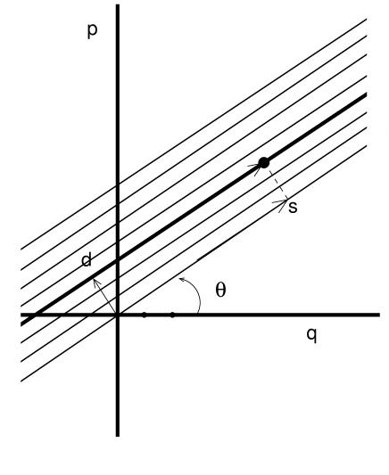
Figure 1: Tomography on the plane.

The Radon transform is defined by

$$F(d,\theta)=\int_{-\infty}^{+\infty}f(s\cos\theta-d\sin\theta,s\sin\theta+d\cos\theta)ds.$$ (5)

The inversion formula, as given by Radon, amounts to consider first the average value of $F$ on all lines tangent to the circle of center $P=(q,p)$ and radius $r$, namely,

$$F_{P}(r)=\frac{1}{2\pi}\int_{0}^{2\pi}F(q\cos\theta+p\sin\theta+r,\theta)d\theta$$ (6)

and then

$$f(q,p)=-\frac{1}{\pi}\int\frac{F^{\prime}_{P}(r)}{r}dr.$$ (7)

The Radon transform maps a (suitable) function on the plane into a function on the cylinder. Some conditions that guarantee the invertibility and continuity of the map were studied by Radon himself Rad1917 , John John , Helgason Helgason and Strichartz Strichartz .

It is possible to write the Radon transform in the affine language (the so-called tomographic map) Rad1917 ; Gelf

$$\omega_{f}(X,\mu,\nu) = \left\langle\delta(X-\mu q-\nu p)\right\rangle$$ (8)

$$= \int_{\mathbb{R}^{2}}f(q,p)\delta(X-\mu q-\nu p)dqdp,$$

where $\delta$ is the Dirac function and the parameters $X,\mu,\nu\in\mathbb{R}$. We notice that

$$\left(\begin{array}[]{cc}\mu&\nu\\ \end{array}\right)\left(\begin{array}[]{cc}1&0\\ 0&1\\ \end{array}\right)\left(\begin{array}[]{c}q\\ p\\ \end{array}\right)=\mu q+\nu p,$$ (9)

but also

$$\left(\begin{array}[]{cc}-\nu&\mu\\ \end{array}\right)\left(\begin{array}[]{cc}0&-1\\ 1&0\\ \end{array}\right)\left(\begin{array}[]{c}q\\ p\\ \end{array}\right)=\mu q+\nu p.$$ (10)

This means that the argument in the Dirac delta function may be considered either as a Euclidean product or as a symplectic product. Equivalently, one might consider the Euclidean or symplectic Fourier transforms.

Another remark is the following. The full linear inhomogeneous group acts transitively on the family of lines on $\mathbb{R}^{2}$. Instead of $\mathrm{E}(2)$ as a privileged group, we may consider

$$\mathrm{SL}(2,\mathbb{R})\equiv\mathrm{Sp}(2,\mathbb{R})\equiv\mathrm{IGL}(2,\mathbb{R})/(\mathbb{R}^{2}\times\mathbb{R}),$$ (11)

where SL, Sp and IGL are the special linear, symplectic and inhomogeneous linear groups, respectively. The $\mathbb{R}$-group in the “denominator” gives dilations while $\mathbb{R}^{2}$ gives translations. Because $\mathrm{Sp}(2,\mathbb{R})$ is not abelian, it can be generated by two types of transformations: rotations

$$\left(\begin{array}[]{cc}\cos\theta&\sin\theta\\ -\sin\theta&\cos\theta\\ \end{array}\right),$$ (12)

and “squeezing” transformations

$$\left(\begin{array}[]{cc}s&0\\ 0&s^{-1}\\ \end{array}\right).$$ (13)

The action of the “squeezing” transformation maps lines into lines, while preserving the area of the triangle. The further action of the rotation group will change the angle formed with the $q$ axis. One may show that the Radon transform is equivariant with respect to the action of $\mathrm{SL}(2,\mathbb{R})$ or $\mathrm{E}(2)$; both of them preserve the measure on $\mathbb{R}^{2}$.

The inverse transform of (8) reads Rad1917 ; Gelf

$$f(q,p) = \int_{\mathbb{R}^{3}}\omega_{f}(X,\mu,\nu)e^{i(X-\mu q-\nu p)}\frac{dXd\mu d\nu}{(2\pi)^{2}}.\quad$$ (14)

In polar coordinates, $\mu=r\cos\theta$, $\nu=r\sin\theta$, the inversion formula takes the form of the standard inverse Radon transform:

$$f(q,p)=\int_{\mathbb{R}}\int_{0}^{2\pi}\omega_{f}(X,\cos\theta,\sin\theta)K(\theta,q,p)\frac{dXd\theta}{(2\pi)^{2}},$$ (15)

with

$$K(\theta,q,p)=\sin\theta\int_{0}^{\infty}e^{-iqr\cos\theta-ipr\sin\theta}rdr$$ (16)

and where we made use of the homogeneity of $\omega_{f}(X,\mu,\nu)$

$$\omega_{f}(\lambda X,\lambda\mu,\lambda\nu)=\frac{1}{|\lambda|}\omega_{f}(X,\mu,\nu),$$ (17)

that is a direct consequence of (8). If the function $f(q,p)$ is a probability density distribution on the phase space of a classical particle, i.e.

$$f(q,p)\geq 0,\quad\int_{\mathbb{R}^{2}}f(q,p)dqdp=1,$$ (18)

also the function $\omega_{f}(X,\mu,\nu)$ is nonnegative and is called a symplectic tomogram or the “Radon component” of the distribution function $f(q,p)$ (analogously to the Fourier component of a function). The Radon component contains the same information on the state of the particle evolving on the phase space as the initial distribution function. Summarizing:

$$\omega_{f}(X,\mu,\nu)\geq 0,\quad\int_{\mathbb{R}}\omega_{f}(X,\mu,\nu)dX=1,\quad\forall\mu,\nu,$$ (19)

the family of tomograms depends on the two real parameters $\mu$ and $\nu$.

III Tomography on the circle

In order to extend the preceding tomographic analysis to particles confined to compact domains there are two alternative definitions, following two different strategies.

III.1 First definition: tomography on the strip

Let us choose for definiteness an interval of width $2\pi$. The configuration space

$$I=[0,2\pi)$$ (20)

yields the phase space $I\times\mathbb{R}$ (a strip). To consider this case it is convenient to deal with the parametrization of lines given by $\mathbb{S}\times\mathbb{R}$, where $\mathbb{R}$ is the translation along the normal to the line. If we consider the intersection of the lines with the selected strip, it is still possible to consider the treatment of the planar situation, where in addition the measure $dqdp$ is multiplied by the characteristic function of the strip.

The state of a classical particle moving in the interval in the presence of fluctuations is associated with a distribution function $f(q,p)\geq 0$, satisfying the normalization condition

$$\int_{I\times\mathbb{R}}f(q,p)dqdp=1.$$ (21)

In this case, the symplectic tomogram (8) specializes to

$$\omega_{f}(X,\mu,\nu)=\int_{I\times\mathbb{R}}f(q,p)\delta(X-\mu q-\nu p)dqdp,$$ (22)

with $X,\mu,\nu\in\mathbb{R}$. One easily checks nonnegativity and normalization like in Eq. (19):

$$\omega_{f}(X,\mu,\nu)\geq 0,\quad\int_{\mathbb{R}}\omega_{f}(X,\mu,\nu)dX=1,\quad\forall\mu,\nu.$$ (23)

The inverse transform, still given by (14), yields a function

$$f(q,p)=\chi_{I}(q)f(q,p)$$ (24)

($\chi_{I}$ being the characteristic function), that vanishes identically outside the strip, i.e. $f(q,p)=0$ for $q\notin I$.

On the other hand, a function $f$ on the strip $I\times\mathbb{R}$ can be extended to a periodic function $f_{2\pi}$ over the whole plane $\mathbb{R}^{2}$ defined by

$$f_{2\pi}(q,p) = \sum_{k\in\mathbb{Z}}f(q-2\pi k,p)$$ (25)

$$= \sum_{k\in\mathbb{Z}}f(q-2\pi k,p)\chi_{I+2\pi k}(q),$$

where the periodicity, $f_{2\pi}(q+2\pi,p)=f_{2\pi}(q,p)$, is apparent and we used Eq. (24) in the second equality.

The phase space has become a cylinder $\mathbb{S}\times\mathbb{R}$, where $\mathbb{S}=\mathbb{R}/(2\pi\mathbb{Z})$ is the unit circle. In order to emphasize this change of geometry, we will denote the position of a particle on the circle by the angle $\phi$ and its angular momentum by $J$. The state of a classical particle moving on the circle in the presence of fluctuations is associated with the distribution function (25) $f(\phi,J)=f_{2\pi}(q=\phi,p=J)$, satisfying the normalization condition

$$\int_{\mathbb{S}\times\mathbb{R}}d\phi dJf(\phi,J)=1.$$ (26)

Due to the periodicity $f(\phi+2k\pi,J)=f(\phi,J)$ ($k\in\mathbb{Z}$), in the inversion formula (14), the Fourier integral over $\mu$ will be replaced by a Fourier series. Therefore, it follows that, in order to reconstruct $f(\phi,J)$, in (22) only the tomograms $\omega_{f}(X,m,\nu)$ with $m\in\mathbb{Z}$ are really needed. Thus, we define

$$\omega_{f}^{(0)}(X,m,\nu)=\langle\delta(X-m\phi-\nu J)\rangle$$

$$\quad=\int_{I\times\mathbb{R}}d\phi dJf(\phi,J)\delta(X-m\phi-\nu J),$$ (27)

where $X,\nu\in\mathbb{R}$ and $m\in\mathbb{Z}$. In Eq. (27) one integrates along the family of one-step segments of helices: $X=m\phi+\nu J$ with $0<\phi<2\pi$ and $X/\nu-2m\pi/\nu<J<X/\nu$. The choice of this family implies the choice of one particular fiber of the cylinder along which each segment is discontinuous. In fact, observe that if the $\phi$-domain of integration in (27) is changed, say to

$$I_{\alpha}=I+\alpha=[\alpha,2\pi+\alpha),$$ (28)

one gets different families of tomograms labeled by a gauge $\alpha$,

$$\omega_{f}^{(\alpha)}(X,m,\nu)=\int_{I_{\alpha}\times\mathbb{R}}d\phi dJf(\phi,J),$$ (29)

which are related to (27) by

$$\omega_{f}^{(\alpha)}(X,m,\nu)=\omega_{\tau_{\alpha}f}^{(0)}(X-m\alpha,m,\nu),$$ (30)

where $\tau_{\alpha}f(q,p)=f(q+\alpha,p)$ is a horizontal translation of $f$. Notice that, due to the periodicity of $f$, the horizontal tomogram, with $m=0$, is gauge invariant, namely $\omega_{f}^{(\alpha)}(X,0,\nu)=\omega_{f}^{(0)}(X,0,\nu)$. Moreover, all families are obtained by restricting $\alpha\in[0,2\pi)$. In fact one gets

$$\omega_{f}^{(\alpha+2\pi k)}(X,m,\nu)=\omega_{f}^{(\alpha)}(X-2\pi mk,m,\nu),$$ (31)

for $k\in\mathbb{Z}$. The gauge $\alpha$ is the anomaly of the chosen fiber of the cylinder $\mathbb{S}\times\mathbb{R}$. See Fig. 2(a). One easily checks nonnegativity and normalization in the form

$$\omega_{f}^{(\alpha)}(X,m,\nu)\geq 0,\quad\int_{\mathbb{R}}\omega_{f}^{(\alpha)}(X,m,\nu)dX=1,$$

$$\qquad\qquad\forall m,\nu,\alpha.$$ (32)

Let us emphasize again that in these formulas, unlike in Eqs. (19) and (23), $m\in\mathbb{Z}$.

Figure 2: Tomography on the circle: (a) strip; (b) cylinder.

The inverse transform is

$$f(\phi,J)=\sum_{m\in\mathbb{Z}}\int_{\mathbb{R}^{2}}\omega_{f}^{(\alpha)}(X,m,\nu)e^{i(X-m\phi-\nu J)}\frac{dXd\nu}{(2\pi)^{2}}.$$ (33)

Indeed, by making use of the Poisson formula

$$\sum_{m\in\mathbb{Z}}e^{im\phi}=2\pi\sum_{m\in\mathbb{Z}}\delta(\phi-2m\pi)=2\pi\,\delta_{2\pi}(\phi),$$ (34)

where $\delta_{T}$ is the $T$-periodic delta function,

$$\delta_{T}(t)=\delta(t\;(\mathrm{mod}\,T))=\left\{\begin{array}[]{ll}\sum_{k\in\mathbb{Z}}\delta(t-kT),&T\neq 0\\ &\\ \delta(t),&T=0\end{array}\right.,$$ (35)

one gets

$$\sum_{m\in\mathbb{Z}}\int_{\mathbb{R}^{2}}\frac{dXd\nu}{(2\pi)^{2}}e^{i(X-m\phi-\nu J)}\omega_{f}^{(\alpha)}(X,m,\nu)$$ (36)

$$= \int_{I_{\alpha}\times\mathbb{R}}d\psi dKf(\psi,K)\sum_{m\in\mathbb{Z}}\int_{\mathbb{R}^{2}}\frac{dXd\nu}{(2\pi)^{2}}$$

$$\times e^{i(X-m\phi-\nu J)}\delta(X-m\psi-\nu K)$$

$$= \int_{I_{\alpha}\times\mathbb{R}}d\psi dKf(\psi,K)\sum_{m\in\mathbb{Z}}\frac{e^{im(\psi-\phi)}}{2\pi}\delta(K-J)$$

$$= \int_{I_{\alpha}\times\mathbb{R}}d\psi dKf(\psi,K)\delta_{2\pi}(\psi-\phi)\delta(K-J)$$

$$= f(\phi,J),$$

as required.

III.2 Second definition: tomography on the cylinder

When we restrict our attention to periodic functions, we are identifying the line at $0$ with the line at $2\pi$. In this way lines become helices. In this situation, however, a new phenomenon takes place: translations along the “normal” will map the helix into itself, for translations which are integer multiples of $2\pi\tan\theta$ (See Fig. 3). The set of different helices is, therefore, parametrized by an angle $\theta\in(-\pi,0)$ and the intercept $\phi\in[0,2\pi)$. Notice that the value $\theta=0$ does not correspond to an helix but to an infinite family of circles “parallel” to the base circle. Thus, the set of helices is a trivial bundle with fiber $\mathbb{S}$ and base manifold $\mathbb{S}\backslash\{0\}$. where we can use as coordinates the slope and intercept $(\theta,\phi)$ or the slope and the shift with respect to the helix crossing the origin i.e. $(\theta,r(\phi,\theta))$ with $r(\phi,\theta)=(2\pi-\phi)\tan\theta$ .

Figure 3: Phase space and relevant variables for the tomography on the strip.

Thus, in this setting we would define the Radon transform as going from functions on $[0,2\pi]\times\mathbb{R}$ to functions on $\mathbb{S}\times(\mathbb{S}\backslash\{0\})$ . It seems clear that only specific applications may suggest to use one or the other. For X-ray tomography the integration along “segments” may be appropriate. For quantum tomography we may want to integrate along maximal Lagrangian submanifolds to get the marginals along transversal Lagrangian submanifolds out of the Wigner function on the full phase space.

For these reasons we introduce a different tomographic probability distribution: let

$$\tilde{\omega}_{f}(X,m,\nu)=\langle\delta_{2\pi m}(X-m\phi-\nu J)\rangle$$

$$=\int_{\mathbb{S}_{1}\times\mathbb{R}}d\phi dJf(\phi,J)\delta_{2\pi m}(X-m\phi-\nu J),$$ (37)

where $X,\nu\in\mathbb{R}$, $m\in\mathbb{Z}$ and $\mathbb{S}_{1}=\mathbb{S}$ is the unit circle. Observe that (37) is independent of the $\phi$-domain of integration, due to the periodicity of the integrand. By plugging (35) into (37) we get for $m\in\mathbb{Z}\backslash\{0\}$ (and an arbitrary $\alpha\in\mathbb{R}$)

$$\tilde{\omega}_{f}(X,m,\nu) = \int_{I_{\alpha}\times\mathbb{R}}d\phi dJ$$ (38)

$$\times f(\phi,J)\sum_{k\in\mathbb{Z}}\delta(X-m\phi-\nu J-2\pi mk)$$

$$= \sum_{k\in\mathbb{Z}}\int_{(I_{\alpha}+2\pi k)\times\mathbb{R}}d\phi dJ$$

$$\times f(\phi-2\pi k,J)\delta(X-m\phi-\nu J)$$

$$= \int_{\mathbb{R}^{2}}d\phi dJf(\phi,J)\delta(X-m\phi-\nu J),$$

while, for $m=0$,

$$\tilde{\omega}_{f}(X,0,\nu)=\int_{\mathbb{S}_{1}\times\mathbb{R}}d\phi dJf(\phi,J)\delta(X-\nu J).$$ (39)

In conclusion, here we integrate over the whole helix, while the previous Eq. (29) was integrated on a single step of it. Notice also that translations along the line $X-m\phi-\nu J$ preserve the measure. By using the homogeneity in Eq. (37) we may consider the quantity $X/m-\phi-(\nu/m)J$ that implies $2\pi m$-periodicity of $\tilde{\omega}_{f}$,

$$\tilde{\omega}_{f}(X+2\pi m,m,\nu)=\tilde{\omega}_{f}(X,m,\nu).$$ (40)

Therefore, the tomogram lives on a family of cylinders labeled by the integer $m$. See Fig. 2(b).

The inverse transform is given by

$$f(\phi,J)=\sum_{m\in\mathbb{Z}}\int_{\mathbb{S}_{m}\times\mathbb{R}}\tilde{\omega}_{f}(X,m,\nu)e^{i(X-m\phi-\nu J)}\frac{dXd\nu}{(2\pi)^{2}},$$ (41)

where $\mathbb{S}_{-m}=\mathbb{S}_{m}=\mathbb{R}/(2\pi m\mathbb{Z})$ is the circle of radius $|m|$ and $\mathbb{S}_{0}=\mathbb{R}$ the real line. When $f$ is nonnegative and normalized as in (26), one easily obtains

$$\tilde{\omega}_{f}(X,m,\nu)\geq 0,\quad\int_{\mathbb{S}_{m}}\tilde{\omega}_{f}(X,m,\nu)dX=1,\quad\forall m,\nu.\$$ (42)

The proof of Eq. (41) goes as follows

$$\sum_{m\in\mathbb{Z}}\int_{\mathbb{S}_{m}\times\mathbb{R}}\frac{dXd\nu}{(2\pi)^{2}}e^{i(X-m\phi-\nu J)}\tilde{\omega}_{f}(X,m,\nu)$$ (43)

$$= \int_{\mathbb{S}_{1}\times\mathbb{R}}d\psi dKf(\psi,K)\sum_{m\in\mathbb{Z}}\int_{\mathbb{S}_{m}\times\mathbb{R}}\frac{dXd\nu}{(2\pi)^{2}}$$

$$\times e^{i(X-m\phi-\nu J)}\delta_{2\pi m}(X-m\psi-\nu K)$$

$$= \int_{\mathbb{S}_{1}\times\mathbb{R}}d\psi dKf(\psi,K)$$

$$\times\sum_{m\in\mathbb{Z}}\int_{\mathbb{R}^{2}}\frac{dXd\nu}{(2\pi)^{2}}e^{i(X-m\phi-\nu J)}\delta(X-m\psi-\nu K)$$

$$= \int_{\mathbb{S}_{1}\times\mathbb{R}}d\psi dKf(\psi,K)\sum_{m\in\mathbb{Z}}\frac{e^{im(\psi-\phi)}}{2\pi}\delta(K-J)$$

$$= \int_{\mathbb{S}_{1}\times\mathbb{R}}d\psi dKf(\psi,K)\delta_{2\pi}(\psi-\phi)\delta(K-J)$$

$$= f(\phi,J),$$

where we made use of Poisson formula (34) and of the equality

$$\sum_{m\in\mathbb{Z}}\int_{\mathbb{S}_{m}}dXe^{i(X-m\phi-\nu J)}\delta_{2\pi m}(X-m\psi-\nu K)$$ (44)

$$= \sum_{m\in\mathbb{Z}}\int_{\mathbb{R}}dXe^{i(X-m\phi-\nu J)}\delta(X-m\psi-\nu K).$$

It is easy to see how the transforms (29) and (37) are related. Indeed, for $m\in\mathbb{Z}\backslash\{0\}$ we get from (38)

$$\tilde{\omega}_{f}(X,m,\nu)=\sum_{r\in\mathbb{Z}}\omega_{f}^{(\alpha)}(X-2\pi mr,m,\nu),$$ (45)

while, from (39)

$$\tilde{\omega}_{f}(X,0,\nu)=\omega_{f}^{(\alpha)}(X,0,\nu).$$ (46)

Incidentally, this relation can be used to give an alternative proof of the inversion formula (41). In fact, from the equality

$$\int_{\mathbb{S}_{m}}\tilde{\omega}_{f}(X,m,\nu)e^{iX}dX$$ (47)

$$= \sum_{r\in\mathbb{Z}}\int_{[\alpha,\alpha+2\pi m)}\omega_{f}^{(\alpha)}(X-2\pi mr,m,\nu)e^{iX}dX$$

$$= \int_{\mathbb{R}}\omega_{f}(X,m,\nu)e^{iX}dX,$$

which is trivially valid for $m=0$, the inversion formula (33) translates into (41).

III.3 A few comments

A few comments are in order. If the configuration space is an interval, the phase space will be a strip and a “free” particle bouncing back and forth will move on a rectangle. If we impose periodic boundary conditions we get circles parallel to the base. Clearly, if we want to consider the quantum case, we have to integrate the Wigner function on Lagrangian subspaces and get the marginals, out of which we should be able to “reconstruct” the function. As we know, we need a “large” family of such marginals, perhaps parametrized by the symplectic group, to be able to reconstruct the “state,” i.e. the original Wigner function Wig32 ; Moyal ; Hillary84 ; Marmoopen ; MarmoPL . This viewpoint differs from the original Radon formulation based on the set of geodesic lines of the plane $\mathbb{R}^{2}$ as Riemannian space (for the two dimensional case), whereas in our case the relevant lines are the Lagrangian lines of the symplectic plane as phase space of the one dimensional particle. In the Radon case the picture is dynamical while in the symplectic case is purely kinematical.

In our “classical” setting, we asked a similar question, i.e. how to reconstruct a classical distribution function on phase space by means of its integrals on a family of one-dimensional subspaces. In some sense the fact that the family is parametrized by two numbers appears as a necessary condition for the reconstruction to be possible.

Finally, it appears that the two ansatz considered in this section yield two different phase spaces. It is reasonable to expect that what is a suitable function in one situation, need not be suitable for the other one. Therefore the two proposals may coexist, once it is clear that they represent different physical situations. In general, they will yield different results. In a way, physics will decide which transform better matches the problem at hand.

IV Gaussian example

Let us consider as an illustration the particular case

$$f(\phi,J)=\frac{1}{(2\pi)^{3/2}}e^{-J^{2}/2},$$ (48)

which is properly normalized, $\int_{\mathbb{S}\times\mathbb{R}}f=1$. The Radon transform (27) yields for $m\neq 0$

$$\omega_{f}^{(\alpha)}(X,m,\nu) = \int_{I_{\alpha}\times\mathbb{R}}\frac{d\phi\,dJ}{(2\pi)^{3/2}}\,e^{-\frac{J^{2}}{2}}\delta(X-m\phi-\nu J)$$ (49)

$$= \frac{1}{|\nu|}\int_{I_{\alpha}}\frac{d\phi}{(2\pi)^{3/2}}\exp\left(-\frac{(m\phi-X)^{2}}{2\nu^{2}}\right)$$

$$= \frac{1}{4\pi|m|}\frac{2}{\sqrt{\pi}}\int_{\frac{|m|}{\sqrt{2}|\nu|}\left(\alpha-\frac{X}{m}\right)}^{\frac{|m|}{\sqrt{2}|\nu|}\left(\alpha-\frac{X}{m}+2\pi\right)}dx\;e^{-x^{2}}$$

$$= \frac{1}{4\pi|m|}\left[\mathrm{erf}\left(\frac{|m|}{\sqrt{2}|\nu|}\left(\alpha-\frac{X}{m}+2\pi\right)\right)\right.$$

$$\left.-\mathrm{erf}\left(\frac{|m|}{\sqrt{2}|\nu|}\left(\alpha-\frac{X}{m}\right)\right)\right],$$

where $\mathrm{erf}(x)$ is the error function. On the other hand, if $m=0$,

$$\omega_{f}^{(\alpha)}(X,0,\nu) = \int_{I_{\alpha}\times\mathbb{R}}\frac{d\phi\,dJ}{(2\pi)^{3/2}}\,e^{-\frac{J^{2}}{2}}\delta(X-\nu J)$$ (50)

$$= \frac{1}{(2\pi)^{1/2}|\nu|}\exp\left(-\frac{X^{2}}{2\nu^{2}}\right).$$

It is easy to verify that the inverse Radon transform (33) permits to recover the original function (48).

On the other hands, the tomograms along the helices read ($m\neq 0$)

$$\tilde{\omega}_{f}(X,m,\nu) = \int_{\mathbb{S}_{1}\times\mathbb{R}}\frac{d\phi\,dJ}{(2\pi)^{3/2}}\,e^{-\frac{J^{2}}{2}}\delta_{2\pi}(X-m\phi-\nu J)$$ (51)

$$= \int_{\mathbb{R}^{2}}\frac{d\phi\,dJ}{(2\pi)^{3/2}}\,e^{-\frac{J^{2}}{2}}\delta(X-m\phi-\nu J)$$

$$= \frac{1}{|\nu|}\int_{\mathbb{R}}\frac{d\phi}{(2\pi)^{3/2}}\exp\left(-\frac{(m\phi-X)^{2}}{2\nu^{2}}\right)$$

$$= \frac{1}{2\pi|m|},$$

while, for $m=0$ it coincides with (50), $\tilde{\omega}_{f}(X,0,\nu)=\omega_{f}^{(\alpha)}(X,0,\nu)$. Note that Eqs. (49) and (51) satisfy (45).

It is clear from this example that the two transforms are different. As we stressed before, both being mathematically legitimate, a choice should be motivated on physical grounds.

V Torus tomography

The generalization to many particles is straightforward. Let us consider $N>1$ classical particles, each moving on its own circle. The system state is described by a probability distribution function $f(\vec{\phi},\vec{J})\geq 0$ satisfying the normalization condition

$$\int_{\mathbb{T}^{N}\times\mathbb{R}^{N}}d\vec{\phi}d\vec{J}f(\vec{\phi},\vec{J})=1,$$ (52)

with coordinates $\vec{\phi}=(\phi_{1},\ldots,\phi_{N})\in\mathbb{T}^{N}=\left(\mathbb{S}\right)^{N}$ on the $N-$torus and angular momenta $\vec{J}=(J_{1},\ldots,J_{N})\in\mathbb{R}^{N}$.

The tomogram of the torus is defined by

$$\omega_{f}^{(0)}(\vec{X},\vec{m},\vec{\nu})=\left\langle\prod_{k=1}^{N}\delta(X_{k}-m_{k}\phi_{k}-\nu_{k}J_{k})\right\rangle$$

$$=\int_{I^{N}\times\mathbb{R}^{N}}\!\!\!\!d\vec{\phi}d\vec{J}f(\vec{\phi},\vec{J})\prod_{k=1}^{N}\delta(X_{k}-m_{k}\phi_{k}-\nu_{k}J_{k}),\qquad$$ (53)

with $\vec{X},\vec{\nu}\in\mathbb{R}^{N}$ and $\vec{m}\in\mathbb{Z}^{N}$. The inverse transform reads

$$f(\vec{\phi},\vec{J}) = \sum_{\vec{m}\in\mathbb{Z}^{N}}\int_{\mathbb{R}^{2N}}\frac{d\vec{X}d\vec{\nu}}{(2\pi)^{2N}}$$ (54)

$$\quad\times\omega_{f}^{(0)}(\vec{X},\vec{m},\vec{\nu})\prod_{k=1}^{N}e^{i(X_{k}-m_{k}\phi_{k}-\nu_{k}J_{k})}.\quad$$

The tomograms $\omega^{(\vec{\alpha})}(\vec{X},\vec{m},\vec{\nu})$ and $\tilde{\omega}(\vec{X},\vec{m},\vec{\nu})$ are obtained analogously, as $N$ dimensional generalizations of (29) and (37).

VI Limit to the standard Radon transform

Let us discuss now how the formulas for the Radon transform (and its inverse) of a function defined on a cylinder tend to those of the standard Radon transform of a function defined on the plane in the limit of infinite radius of the cylinder. To this end, let us first recall how the Fourier series of a periodic function $f_{R}(q)$ with period $R$ and normalization $\int_{-R/2}^{R/2}f_{R}(q)dq=1$ becomes the Fourier integral when $R\to\infty$. The Fourier series reads

$$f_{R}(q)=\sum_{m\in\mathbb{Z}}C_{k_{m}}e^{-ik_{m}q},\qquad k_{m}=\frac{2\pi}{R}\,m,\qquad(m\in\mathbb{Z})$$ (55)

and its coefficients are given by

$$C_{k_{m}}(R)=\frac{1}{R}\int_{-R/2}^{R/2}f_{R}(q)e^{i2\pi mq/R}\,dq.$$ (56)

For $R\to\infty$ the Fourier series becomes the Fourier integral representation of the function $f(q)=\lim_{R\to\infty}f_{R}(q)$ defined on the line. Thus Eq. (55) becomes

$$f(q) = \lim_{R\to\infty}\sum_{m\in\mathbb{Z}}\Delta k\frac{R}{2\pi}\,C_{k_{m}}e^{-ik_{m}q}$$ (57)

$$= \int_{-\infty}^{\infty}C(k)e^{-ikq}\,dk,$$

where $\Delta k=k_{m+1}-k_{m}=2\pi/R$, and $C(k)=\lim C_{k_{m}}R/2\pi$. On the other hand, Eq. (56) takes the form

$$C(k)=\lim_{R\to\infty}\frac{R}{2\pi}\,C_{k_{m}}=\frac{1}{2\pi}\int_{-\infty}^{\infty}f(q)e^{ikq}\,dq.$$ (58)

Using these well known limiting relations one can get the limit of the tomographic map formulae for the particle moving on the circle. For definiteness we will look at the tomogram (27); the procedure is analogous for the other tomograms. We first replace Eq. (27) by a formula that takes into account the radius $R$ of the circle. Given a probability density $f(\phi,J)\geq 0$ on the cylinder, by introducing the new variables $q=\phi R/2\pi$ and $p=J$ and setting

$$f_{R}(q,p)=\frac{2\pi}{R}f\left(\frac{2\pi q}{R},p\right),$$ (59)

we have the tomogram (27) in the form

$$\omega_{f}^{(0)}(X,\mu_{m},\nu)=\langle\delta(X-\mu_{m}q-\nu p)\rangle$$

$$=\int_{-R/2}^{R/2}\int_{-\infty}^{\infty}f_{R}(q,p)\delta(X-\mu_{m}q-\nu p)\,dq\,dp,\quad$$ (60)

where $\mu_{m}=2\pi m/R$ with a correctly normalized probability density

$$\int_{-R/2}^{R/2}\int_{-\infty}^{\infty}f_{R}(q,p)\,dq\,dp=1.$$ (61)

The inverse formula (33) reads

$$f_{R}(q,p)=\sum_{m\in\mathbb{Z}}\Delta\mu\int_{\mathbb{R}^{2}}\omega_{f}^{(0)}(X,\mu_{m},\nu)e^{i(X-\mu_{m}q-\nu p)}\frac{dXd\nu}{(2\pi)^{2}},$$ (62)

with $\Delta\mu=2\pi/R$. In the limit $R\to\infty$, we get formulae (8) and (14) and the tomographic map on the circle yields the Radon transform on the plane.

VII Conclusions and perspectives

We have shown that one can map the probability distribution density $f(\phi,J)$, defined on a cylinder in terms of two random variables (position $\phi$ and angular momentum $J$), onto a family of probability distribution densities depending on one random variable $X$, which is a continuous coordinate on the helix. The family of helices is labelled by the integer number $m$ and the real number $\nu$. The map is obtained by means of the Radon transform extended to the case of a cylinder.

The Radon transform is closely related to the Fourier transform. We pointed out an important specific property of the Radon transform, that is valid both for tomographic maps of functions defined on the plane and on the cylinder: in contrast to the Fourier transform, for which the Fourier component of the probability density is not a probability density, the Radon component of the probability density (given on the plane or the cylinder) is again a probability density and depends on some extra parameters.

We have also straightforwardly extended the Radon transform construction to the classical motion on a multidimensional torus and shown that the tomographic map of probability densities on cylinder becomes the tomographic map of probability density on the plane. This implies that the two corresponding Radon transforms are related to each other, in close analogy to the relation between Fourier series and Fourier integrals for functions on a circle and functions on a line. One difference should be stressed though: while in the Fourier case the limit is taken in $L^{2}$, in the Radon case it is (obviously) taken in $L^{1}$. This is apparent in the manipulations of Sec. VI.

The quantum extension of the tomographic map for the free motion on a circle requires additional investigation, due to the well-known ambiguities in the definition of the analogues of the conjugate observables angle and angular momentum hradilangle . Similarly, the extension of Radon transforms for curved manifolds in the present and related contexts deserves additional study Helgason .

- (1) J. Radon, Über die bestimmung von funktionen durch ihre integralwerte längs dewisse mannigfaltigkeiten, Breichte Sachsische Akademie der Wissenschaften, Leipzig, Mathematische-Physikalische Klasse, 69 S. 262 (1917).
- (2) E. P. Wigner, Phys. Rev. 40, 749 (1932).
- (3) J Moyal, Proc. Camb. Phil. Soc. 45, 99 (1949).
- (4) M. Hillary, R. F. O’Connell, M. O. Scully, and E. Wigner, Phys. Rep. 106, 121 (1984).
- (5) J. Bertrand and P. Bertrand, Found. Phys. 17, 397 (1987).
- (6) K. Vogel and H. Risken, Phys. Rev. A 40, 2847 (1989).
- (7) S. Mancini, V. I. Man’ko and P. Tombesi, Quantum Semiclass. Opt. 7, 615 ( 1995).
- (8) O. V. Man’ko and V. I. Man’ko, J. Russ. Laser Res. 18, 407 (1997).
- (9) V. I. Man’ko and R. V. Mendes, Physica D 145, 222 (2000).
- (10) P. Banáš, J. Řeháček, and Z. Hradil, Phys. Rev. A 74, 014101 (2006); Z. Hradil, D. Mogilevtsev, and J. Řeháček, Phys. Rev. Lett. 96, 230401 (2006).
- (11) D. T. Smithey, M. Beck, M. G. Raymer, and A. Faridani, Phys. Rev. Lett. 70, 1244 (1993).
- (12) G. Zambra, A. Andreoni, M. Bondani, M. Gramegna, M. Genovese, G. Brida, A. Rossi, and M. G. A. Paris, Phys. Rev. Lett. 95, 063602 (2005); M. Genovese, G. Brida, M. Gramegna, M. Bondani, G. Zambra, A. Andreoni, A.R. Rossi, M.G.A. Paris, Laser Physics 16, 385 (2006); G. Brida, M. Genovese, F. Piacentini, Matteo G. A. Paris, Optics Letters, 31, 3508 (2006).
- (13) C. Kurtsiefer, T. Pfau, and J. Mlynek, Nature 386, 150 (1997).
- (14) G. Badurek, et al, Physical Review A 73, 032110 (2006).
- (15) Quantum State Estimation, Lecture Notes in Physics Vol. 649, edited by M. G. A. Paris and J. Řeháček (Springer, Berlin, 2004).
- (16) G. M. D’Ariano, S. Mancini, V. I. Man’ko and P. Tombesi, Quantum Semiclass. Opt. 8, 1017 (1996).
- (17) O. V. Man’ko, V. I. Man’ko and G. Marmo, J. Phys. A: Math. Gen. 35, 699 (2002).
- (18) O. V. Man’ko, V. I. Man’ko and G. Marmo, Phys. Scr. 62, 446 (2000).
- (19) F. John, Plane waves and spherical means: Applied to Partial Differential Equations (Wiley Interscience, New York, 1955).
- (20) S. Helgason, Ann. of Math. 98, 451 (1973); Groups and Geometric Analysis (Academic Press, Orlando, 1984); The Radon Transform (Birkhauser, Boston, 1980).
- (21) R. S. Strichartz, American Mathematical Monthly 89, 377 (1982).
- (22) I. M. Gel’fand and G. E. Shilov, Generalized Functions: Properties and Operations, Vol. 5 (Academic Press, 1966)
- (23) V. I. Man’ko, G. Marmo, A. Simoni and F. Ventiglia, Open Sys. & Information Dyn. 13, 239 (2006).
- (24) V. I. Man’ko, G. Marmo, A. Simoni, A. Stern and E.C.G. Sudarshan, Phys. Lett. A 35, 351 (2005).
- (25) Z. Hradil, J. Rehacek, Z. Bouchal, R. Celechovsky, and L. L. Sanchez-Soto, Phys. Rev. Lett. 97, 243601 (2006).