Classical and quantum three-dimensional
integrable systems with axial symmetry
M. Gadella∗, J. Negro∗ and G. P. Pronko†
∗Departamento de Física Teórica, Atómica y
Óptica
Universidad de Valladolid, E-47005, Valladolid, Spain
†Institute of High Energy Physics, Protvino,
Moscow Region, 148280, Russia.
Institute of Nuclear Physics, NCSR, “Demokritos”, Athens, Greece.
Abstract
We study the most general form of a three dimensional classical integrable system with axial symmetry and invariant under the axis reflection. We assume that the three constants of motion are the Hamiltonian, , with the standard form of a kinetic part plus a potential dependent on the position only, the -component of the angular momentum, , and a Hamiltonian-like constant, , for which the kinetic part is quadratic in the momenta. We find the explicit form of these potentials compatible with complete integrability. The classical equations of motion, written in terms of two arbitrary potential functions, is separated in oblate spheroidal coordinates. The quantization of such systems leads to a set of two differential equations that can be presented in the form of spheroidal wave equations.
1 Introduction
This is a paper on integrability of three dimensional systems, both classical and quantum. Apart from being interesting by itself, this study can be extremely interesting for a field, which is rather far away from the present subject, the theory of the continuous media: gas, fluid and plasma. Those are mechanical systems with an infinite number of degrees of freedom and certainly much more difficult than the mechanics of a particle in three dimensions. However, in the theory of continuous media, we can pose a problem of the existence of solitons: the steady solution with time-independent field with density and velocities . It could exist in the non dissipative case only, as we neglect the viscosity. In this latter case, the particles which constitute the media should move in a self consistent potential along its trajectories, which should be closed. Although this potential is the result of interparticle interaction, each single particle moves in an effective potential that provides the closed trajectory. From the analysis of the equations of motion in continuous media ([1]), it follows that the simplest shape of solution is a toroid. Thus, we have to look for a three dimensional single particle integrable system including a toroidal shape. One of the goals of the present paper is to make a first step in this direction, as we describe all completely integrable systems with axial symmetry. The next step would be to select among all the completely integrable systems those sharing some specific properties.
2 The axial coordinates
Let us consider a three dimensional classical system with the canonical coordinates , , where the commutators are defined by the usual Poisson brackets , the sum being understood over repeated indexes. The evolution of the system is described by the Hamiltonian
| (2.1) |
where is a potential term. Let us assume the existence of two additional integrals of motion for this system, all of them in involution. The first one will be chosen as the angular momentum along the direction fixed by the unit vector :
| (2.2) |
As for the second one we require to be quadratic in momentum and commuting with both, and . Then, it is straightforward to show that, provided we include also the reflection with respect to the -axis as a discrete symmetry of our system, it must take the general expression:
| (2.3) |
where the quadratic term has the ‘metric’
| (2.4) |
being a real constant that we take positive. The quadratic term in the momenta can be written as
| (2.5) |
where is the perpendicular component of to the -axis, and . Here we must point out that the operators (2.2) and (2.5) determine the prolate-oblate spheroidal coordinates that separate the Laplacian operator [9].
The commutation of with and restrict the form of their potential terms
| (2.6) |
while the commutation of and leads to the equations
| (2.7) |
In order to deal with (2.7) we diagonalize the matrix . Its eigenvalues and eigenvectors are obtained from the matrix equation
| (2.8) |
We get the solutions
| (2.9) |
The corresponding eigenvectors can be expressed in the following way:
| (2.10) |
where is the azimutal angle around the -axis. Let us write here some useful identities of these eigenvalue functions for future calculations,
| (2.11) |
Since the eigenvectors (2.10) are orthogonal, it is natural to adopt as new orthogonal coordinates the set , which are essentially the oblate spheroidal coordinates [9]. We turn to eq. (2.7) for the potentials, now expressed in the new coordinate system. Taking into account that due to the geometric symmetry, (2.2), and do not depend on , (2.7) becomes
| (2.12) |
where stand for . Now, as is diagonal in the new coordinate basis , this equation decouples in
| (2.13) |
or
| (2.14) |
This means that
| (2.15) |
where and are arbitrary functions. The minus sign in the front of (2.15) intends that the next equations, derived from (2.15), can be written in a symmetric form with respect to the variables and . These equations give an expression for the potentials as follows:
| (2.16) |
These are the most general expressions for the potentials and compatible with .
3 Separation of variables
3.1 The momentum as a gradient
Now we will recall here a property for a classical system in three dimensions having three integrals of motion (including the Hamiltonian) , , in involution, thus being integrable:
| (3.17) | |||
| (3.18) |
If we assume that the determinant of the matrix is nonvanishing, the inverse function theorem gives from (3.17) the expression of the momenta as functions of coordinates, at least locally:
| (3.19) |
so that
| (3.20) |
Taking partial derivatives of this equation, we obtain
| (3.21) | |||
| (3.22) | |||
| (3.23) |
Note that the second identity in (3.22) comes after condition (3.18). According to our hypothesis, the determinant of the matrix vanishes, so that the last relation can be simplified:
| (3.24) |
From (3.21) and (3.24) we have
| (3.25) |
hence
| (3.26) |
This means that the vector field, in the variable , has vanishing rotational, i.e.,
| (3.27) |
Therefore, if is sufficiently regular, there exists a function , locally defined, such that
| (3.28) |
In conclusion, we have shown that if there are three integrals of motion (3.17) in involution, the momentum will be the gradient of the function :
| (3.29) |
These could be considered as a first class constraints. The function is the characteristic function in the Hamilton-Jacobi approach. Note that this is a general property, valid for any dimension .
3.2 The separation of
We can apply the above results to our system by making the identification , , . The next step is to show the separability of the function in the variables introduced in the previous section. Then, if we apply the chain rule to (3.28) and make use of (2.10), we have
| (3.30) |
Since the vector fields in (2.10) are mutually orthogonal, multiplying both sides of the above expression by , we obtain
| (3.31) |
where is the value of the integral of motion corresponding to the angular momentum around . We conclude that
| (3.32) |
and therefore taking the square modulus in (3.32), we have that
| (3.33) |
where is the value of the constant of motion . We recall that the expression (3.32) for the momentum vector field has been obtained in the basis that diagonalizes the metric matrix of components . In this basis and from (3.32), we straightforwardly compute:
| (3.34) |
where is the value of .
Next, we multiply equation (3.33) by , (3.34) by and sum. Next we make the same procedure with instead. Finally, we get the following two expressions:
| (3.35) |
Taking into account the definition (2.9) of , the next formulas are easily obtained:
| (3.37) |
We finally have
| (3.38) |
Now, let us observe that in the right hand side of (3.38) the combination cannot depend on . At the same time, will not depend on . Note that a similar behavior have arosen in (2.14). Hence, since and depends only on and , respectively, while the dependence on was given by (3.31), we conclude that we have managed to obtain the separation of in the variables , i.e.,
| (3.39) |
Later, we shall find an explicit form for in terms of a different set of variables.
3.3 The integration of the equations of motion
Our next objective is the integration of the following equations of motion:
| (3.40) |
In other words, our goal is finding the explicit dependence of the variables and with time, i.e., the functions and . From (3.38) and (3.39), it is clear that
| (3.43) |
where the dot denotes time derivative, as usual. Therefore,
| (3.44) |
From the first two equations in (3.44),
| (3.45) |
we can get three expressions separated in , and :
| (3.46) |
If the potentials (2.16) are known, e.g., the functions and are chosen, then the functions and will be also explicitly known. Thus, integrating over time (3.46) we obtain the following crude expressions:
| (3.47) |
These relations constitute an implicit form of the integration of the equations of motion. To obtain the coordinates , and as explicit functions of time we should invert such relations, a task which is not often simple and that will depend on each particular choice of the functions and .
3.4 The function in terms of oblate spheroidal coordinates
From the definition (2.9) is always positive meanwhile the values of lie on the interval , depending on the scalar product . Thus, we suggest the following change of coordinates:
| (3.48) |
Therefore we have
| (3.49) |
where are the usual oblate spherical coordinates [5]-[9]. Here, we shall see how the dependence of in terms of , and gives a new insight into the above discussion. If we take time derivative in (3.48), we obtain:
| (3.50) |
From (3.48), one readily obtains
| (3.51) | |||||
| (3.52) |
Now, we compare the expressions given in (3.43) and (3.48) for and use (3.51) to conclude that
| (3.53) |
An analogous manipulation shows that
| (3.54) |
Using the last formula in (3.44) and (3.48), we find the expression for the time derivative of as
| (3.55) |
Since the functions and depend respectively of and only, they can be written as functions of and , respectively. As and are, in principle, arbitrary, we could denote these functions as and respectively. Thus, (2.15) can be written as (except for an irrelevant change on the sign):
| (3.57) | |||||
| (3.58) |
so that, we finally get the following expressions for the derivatives of and :
| (3.59) | |||||
| (3.60) | |||||
where obviously,
| (3.63) |
where is a constant with respect to time (obviously, it depends on and ). Another constant of motion can be obtained as follows: First, we write (3.55) as
| (3.65) |
From (3.65), we obtain
| (3.66) |
which shows that
| (3.67) |
is a constant of motion.
| (3.68) |
which obviously yields after integration
| (3.69) |
The function can now be written in terms of the variables . Since and are functions of and alone, respectively, formula (3.39) can be written as
| (3.70) |
where
| (3.71) |
This gives the final expression for as
| (3.72) |
Time invariants and can be written in terms of certain partial derivatives of as we can easily show. In fact, using the expressions for and in (3.61) and (3.62), we have that
| (3.73) |
as it can be easily checked. Then, the function can be written as
| (3.74) |
where and are dependent on , and , but they are time independent.
4 Quantum systems
From the point of view of quantum mechanics, the Hamiltonian as well as the integrals of motion and are hermitian operators obtained simply by replacing , , in (2.1), (2.2) and (2.3), respectively (we have taken along this section). Formal hermiticity follows from the fact that the operators , and are symmetric in the usual cartesian coordinates. The kinetic parts of and are nonsingular quadratic expressions on positions and momenta and they are self adjoint ([11]). In addition, we assume that the potentials and satisfy sufficient conditions so that both and be self adjoint (as for example that the conditions in the Kato Rellich theorem be satisfied [12]).
The conditions (2.4) on the metric , and (2.6)-(2.7) on the potential terms guarantee the commutation relations for these operators:
| (4.75) |
We will look for the simultaneous eigenfunctions of the three operators
| (4.76) |
or equivalently
| (4.77) |
where
| (4.78) |
Now, we will express these differential operators in terms of the coordinates in order to rewrite the eigen-equations in the form
| (4.79) |
Taking into account that
| (4.80) |
and also (2.14), equations (4.79) can be written in a separated form,
| (4.81) |
where and appear in the first and second equation in (4.81) respectively. Therefore we can look for a factorized solution for the eigenfunctions as follows:
| (4.82) |
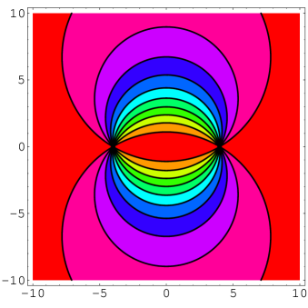
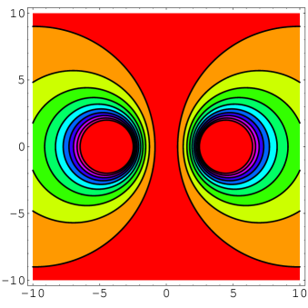
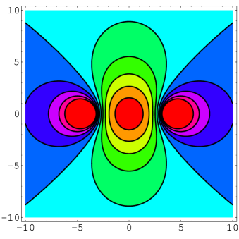
We can go back to the change of coordinates given by (3.48). This change of coordinates is also suggested by the formulas below, as we shall see. Now, it is time for choosing explicit forms for the functions and in (2.15). For , we shall choose the function that vanish identically. For , we choose , where is a constant. Then, the following expressions arise:
| (4.83) |
Or, in cartesian coordinates,
| (4.84) |
Now, we carry (3.48) and (4.83) into (4.81) to get the following set of two differential equations in the variables and :
| (4.85) | |||
| (4.86) |
This is a special type of equations already studied in the literature that we briefly analyze in the next section.
5 Study of the equations and their solutions.
First of all, it seems convenient to simplify equations (4.85-4.86). In order to fulfil this goal, let us choose the following new coordinates:
| (5.87) |
Let us introduce the following parameters:
| (5.89) | |||
| (5.90) |
We observe that in the case of and only in this case, these equations can be reduced to equations of hypergeometric type, which can be solved in terms of hypergeometric functions. However, this is not the most general case, let us consider the following differential equation:
| (5.91) |
where , and are real parameters ( may be positive or negative depending on the use of prolate or oblate coordinates respectively). This is called the spheroidal wave equation [10]. It is very simple to show that both equations (5.89) and (5.90) are versions of the spheroidal wave equation. In fact, (5.90) can be written as
| (5.92) |
with and . If we apply the change of variables given by , equation (5.89) becomes
| (5.93) |
where again and we have kept the notation .
Solutions of the spheroidal wave equation (5.91) and therefore of (5.92) and (5.93) have been studied in [10]. The origin is a regular point of the equation and therefore, we can find two linearly independent functions in terms of powers series on the variable . These series converges on the open circle centered at the origin and radius equal to one, since are singular points for the equation. On this open circle, one can find one even and one odd solution of (5.91) of the form and respectively, which are linearly independent. These series do not converge at the singular points . As they do converge on the open interval , the wave function solution of equation (4.86) is periodic on the real axis with singularities at the points . There exists another type of linearly independent even and odd solutions on a neighborhood of the origin that may converge at the singular points , provided that a relation is satisfied between the coefficients , and in (5.91) (and its corresponding translation in terms of the coefficients in (5.92) and (5.93)) [10]. In any case, the solutions of (4.86) on the real axis are periodic and therefore, not square integrable.
With respect to equation (5.91), are regular singular points with indices equal to . Being an integer, the two linearly independent solutions on a neighborhood of are and with and , where and are power series on . These power series have radii of convergence equal to 2. On a neighborhood of , similar solutions can be found. Power series never truncate.
There is another singular point at . This singular point is irregular. Solutions on a neighborhood of the infinite have the form , where is a complex number depending on the equation parameters. In order to simplify the recurrence relations for the coefficients , it is customary to choose this solution as . The condition that the Laurent series converges in gives a relation between and [10]. These solutions are of the form
| (5.94) |
where
| (5.95) |
with , , and , being and the Bessel functions of first, second and third class respectively. Any two of the set of solutions (5.94) are linearly independent provided that be not a half odd integer.
Solutions of (5.89) and (5.90) can be obtained without resorting to the standard study of the spheroidal wave function. For instance, if we use the change of variables given by in (5.89), this equation is transformed into
| (5.96) |
Now, the singular regular points lie at and it is not difficult to obtain solutions in form of power series on a neighborhood of these points. For example, for the characteristic exponents are and giving respective linearly independent solutions of (5.96) of the form and . Recurrence relations for the coefficients depend on four coefficients, except the first and second relations which depend on the two and three first coefficients respectively (which is compatible with the fact that and should be the only independent coefficients). On a neighborhood of the singular point , two linearly independent solutions can be found of the form and . These series make sense provided that compatibility relations exists between the parameters , and in complete agreement with the general study of the solutions of spheroidal wave functions in [10].
6 Conclusions and remarks.
We have studied the conditions of integrability of a classical or quantum system having a symmetry axis. As in a three dimensional integrable system, we have found three independent observables such that their respective Poisson brackets are zero, in the classical case, or commute in the quantum case. The chosen symmetry forces one of the observables to be the component of the angular momentum in the direction of the symmetry axis. The other two can be written in Hamiltonian form as a sum of a kinetic term plus a potential.
In the classical case, we have obtained the most general form of the potentials corresponding to both Hamiltonians in terms of oblate spheroidal coordinates, that depends on two arbitrary functions depending on one coordinate only. We have written the equations of motion in terms of this coordinates and show that the Hamilton-Jacobi characteristic function can be written as a sum of three functions each one depending on one coordinate only. Then, we have obtained the explicit form for these three functions.
The quantum case is obtained by direct canonical quantization of the classical case. The condition of integrability yields to two Schrödiger type equations in which with separate variables. Then, a reasonable choice on the functions that determine the potentials yields to new equations that are shown to be of the spheroidal type. We finish the discussion with some comments on the solutions of this kind of equations.
Acknowledgments
We are grateful to Profs. M. Ioffe, L.P. Lara and M. Santander for useful comments. Partial financial support is acknowledged to the Junta de Castilla y León Project VA013C05, the Ministry of Education and Science of Spain projects MTM2005-09183 and FIS2005-03988 and Grant SAB2004-0169 and the Russian Science Foundation Grant 04-01-00352.
References
- [1] G.P. Pronko, Thoeretical and Mathematical Physics, 146, (2006) 85.
- [2] L.P. Eisenhart, Ann. Math. 35 (1934) 284; Phys. Rev. 74 87.
- [3] N.W. Evans, Phys. Rev. 41 (1990) 5666; Phys. Lett. 147A (1990) 483; J. Math. Phys. 32 (1991) 3369.
- [4] A.A. Makarov, Ya. Smorodinsky, K. Valiev and P. Winternitz, Nuovo Cim. 52, 1061 (1967)
- [5] J.A. Stratton et al., Spheroidal Wave Functions, Technology Press of M.I.T. and John Wiley & Sons, New York, 1956.
- [6] C. Flammer, Spheroidal Wave Functions, Stanford Univ. Press, Stanford, Calif., 1957.
- [7] J. Meixner and F.W. Schäfke, Mathieusche Funktionen und Sphäroidfunktionen (Mathieu Functions and Spheroidal Functions), Springer- Verlag, Berlin, 1954. J. Meixner, F.W. Schäfke, and G. Wolf, Mathieu Functions and Spheroidal Functions and Their Mathematical Foundations, Springer- Verlag, 1980.
- [8] A. Erd lyi et al., Higher Transcendental Functions, Vol. 3, McGraw-Hill, New York, 1953; reprint edition, Krieger Publishing Co., Malabar, Fla., 1981.
- [9] W. Miller Jr, Symmetry and separation of variables, Addison-Wesley, 1977.
- [10] F.M. Arscott, Periodic Differential Equations, (Pergamon, Oxford, UK 1964).
- [11] M. Gadella, J.M. Gracia Bondía, L.M. Nieto, J.C. Varilly, J. Phys. A: Math. Gen., 22, 2709, (1989).
- [12] M. Reed, B. Simon, Fourier Analysis. Self Adjointness, Academic Press, New York, 1975.