Growth of polyhedral crystals
from supersaturated vapor

Abstract

We examine the growth of crystals from vapor. We assume that the Wulff shape is a prism with a hexagonal base. The Gibbs-Thomson correction on the crystal surface is included in the model. Assuming that the-initial crystal has an admissible shape we show local in time existence of solutions.

Keywords: Free boundary problem; Crystal growth; Gibbs - Thomson relation; Epitaxy

1 Introduction

The main result of this paper is a mathematical study of crystals grown from supersaturated vapor. We assume that evolving crystal $\Omega$ is a prism with $N$-gonal base. We assume that the number $N$ is constant. Let us stress that our crystal $\Omega$ has not to be a convex set (see Figure 1 in the case $N=54$). Such kind of ice crystals are formed in the atmosphere. Our activity is motivated by Gonda and Gomi results, [14], and also by Giga and Rybka [9]. The authors of the paper [9] assumed that the Wulff shape is a fixed cylinder and also that the process was slow, i.e. they considered quasi-steady approximation of  the diffusion equation (diffusion is much faster than the evolution of free boundary). Giga and Rybka obtained results for quasi-steady approximation system (see [10], [11], [12], [13]).

In this paper we do not assume that the crystal evolves slowly. Namely, we assume that supersaturation $\sigma$ fulfills diffusion equation with a drift

$$\varepsilon\frac{\partial}{\partial t}\sigma=\Delta\sigma+f\cdot\nabla\sigma$$ (1)

outside of crystal $\Omega$. For simplicity of notation we assume that $\varepsilon=1$. We are not going to examine the properties of the solution when we change the parameter $\varepsilon$. In the above equation $f$ is a velocity of vapor. We assume that $f$ is given. In fact, velocity $f$ should satisfy an addition equation.

We assume that the supersaturation $\sigma$ has a specific value at infinity, i.e.

$$\lim_{|x|\rightarrow\infty}\sigma(x)=\sigma^{\infty}.$$ (2)

We require that mass conservation law on the crystal surface is fulfilled. Namely,

$$g=\frac{\partial\sigma}{\partial\nu},$$ (3)

where $\nu$ is the outer normal. This condition is very natural in the epitaxy model. See Eliot and Gurtin paper [6]. Let us stress that it could be better to discussed the system with replaced $g$ by $V$ in (3), where $V$ is the velocity of the growing crystal. Namely, $V=\frac{\partial\sigma}{\partial\nu}$. This is the so-called Stefan condition. Our method can not be applied to this case. This problem will be examined in the forthcoming article [15].

The value of the supersaturation $\sigma$ at the surface satisfies Gibbs-Thomson law, namely,

$$-\sigma=-div_{S}\xi-\beta V,$$ (4)

where $\beta$ is the kinetic coefficient and $\xi$ is a Cahn-Hoffman vector field (see [18]). We denote by $V$ the velocity of the growing crystal. We also assume that the velocity $V$ is constant on each side of the crystal. Our model does not include bending and breaking of surface $\partial\Omega$. Roughly speaking the above relation says the supersaturation on the crystal surface is proportional to the curvature of surface ($-div_{S}\xi$), and to the velocity of the evolving crystal. Let us discuss the properties of the Cahn-Hoffman vector field $\xi$. Let $\gamma$ be surface energy density (Finsler metric, see [27]), i.e. $\gamma:\mathbb{R}^{3}\rightarrow\mathbb{R}$ is a $1$-homogeneous, convex and Lipschitz continuous function. If the surface of the crystal $\partial\Omega$ and the surface energy density $\gamma$ are smooth, then

$$\xi(x)=\nabla\gamma(\nu(x)).$$ (5)

If we do not assume that $\gamma$ and $\partial\Omega$ are smooth then the above expression may not make sense (see [8]). Instead $\nabla\gamma$ we can write subdifferential $\partial\gamma$, which is defined everywhere. In this case $\partial\gamma$ is a nonempty convex set (not necessarily singleton). The condition (5) can be replaced by the following relation

$$\xi(x)\in\partial\gamma(\nu(x)).$$

We are not going to discuss the properties of the Cahn-Hoffman vector field. In preliminaries section we show a "nice" property of the averaged divergence of the Cahn-Hoffman field $\xi$, namely

$$-\kappa_{i}\mathcal{H}^{2}(S_{i})=\int_{S_{i}}div_{S}\xi\,d\mathcal{H}^{2}(x),$$

where $\kappa_{i}$ is a crystalline curvature (see next section). Let us stress that the LHS of the above expression is independent of $\xi$.

In this paper we assume that the Frank diagram $F_{\gamma}$ (see [18] or next section) is a sum of two regular pyramids having a common base. Hence, the Wulff shape $W_{\gamma}$ is a prism with a hexagonal base. We assume that the crystal is an admissible shape, i.e. the set of outer normal vectors to $\partial\Omega$ coincides with the set of outer normal vectors to $W_{\gamma}$. Let us notice that $\Omega$ need not be a convex set. Let us stress that we could apply our analysis to more general Wulff shape. Namely, we could assume that $W_{\gamma}$ is a prism with regular $k$-gonal base, where $k\geq 3$. But only hexagonal symmetry is intersting from pysical point of view (see Figure 1).

In order to simplify our system (1), (2), (3), (4) we will consider averaged Gibbs-Thomson law. Taking into account the above considerations and the assumption that the velocity $V$ is constant on each side of the crystal we obtain

$$-\int_{S_{i}}\sigma d\mathcal{H}^{2}=\kappa_{i}\mathcal{H}^{2}(S_{i})-\beta_{i}V_{i}\mathcal{H}^{2}(S_{i}).$$ (6)

Let us mention that averaged Gibbs-Thomson is not new condition. Namely, this equation has appeared in [19] and [21].

Our main aim is to show the local in time existence of solutions to (1), (2), (3), (6). We show this in a few steps. Let us notice that we can look at this system as parabolic equation coupled with ordinary differential equation for the evolving sides of crystal (the signed distance side from $S_{i}(t)$ to $S_{i}(0)$). Next, we transform our problem to the system in the fixed set, in this case it is outside the initial crystal. In this domain we solve our system. Subsequently, we examine the linear problem and here we apply the analytic semigroup theory (see [1], [2], [4], [7], [20], [23]). Next we construct an approximating sequence and apply Ascoli’s Theorem. Let us notice that we work in an unbounded domain and the standard Rellich-Kondrachov compactness theorem does not work. We have to show additional properties of the approximating sequence. Our method is similar to the method presented in [28].

The paper is organized as follows. First, we introduce notations, recall definitions, show some facts about crystalline curvature and formulate the problem. Next, we show the main result. The last section (Appendix) contains useful result.

At the end of this section, let us comment on the mathematical literature. In the smooth case, i.e. assuming that the surface of the crystal is differentiable manifold and for the two phase Stefan problem this model was solved in the class of smooth function (see Chen and Reitich [5]). Independently, Radkevich (see [26]) showed local in time existence of a smooth solution to the problem considered by Chen and Reitich. The advantage of Radkevich is that the author allows a slightly more general form of the diffusion equation. The problem for $\beta=0$ and smooth interfaces was studied by Luckhaus [22] and in greater generality by Almgren-Wang [3]. In particular, they showed that uniqueness fails. Let us stress that these authors have worked in bounded domain. Quasi-steady approximation in the case when the crystal is a cylinder and a domain is unbounded was discussed by Giga and Rybka [9]. Let us mention that these authors discussed the system with replaced $g$ by $V$ in (3), i.e. the so-called Stefan condition. Our method can not be applied to this case.

Notation. We use the following convention, whenever we see the inequality $\mathbb{A}\leq c\mathbb{B}$ we tacitly understand that it holds with some positive constant $c$ independent of $\mathbb{A}$ and $\mathbb{B}$.

2 Preliminaries

Let us denote an evolving crystal by $\Omega(t)$, and its exterior by $\Omega(t)^{c}=\mathbb{R}^{3}\setminus\Omega(t)$. Let $S(t)=\partial\Omega(t)$ its surface. We assume that crystal $\Omega(t)$ is a prism at all times. To be more precise we write

$$\Omega(t)=\{(\tilde{x_{1}},\tilde{x_{2}},\tilde{x_{3}})\in\mathbb{R}^{3}:L_{B}(t)\leq\tilde{x_{3}}\leq L_{T}(t),(\tilde{x_{1}},\tilde{x_{2}})\in W(t)\}.$$

Where $W(t)$ is an $N$-gon in the plane.

Let us divide the surface into $N+2$ pieces, i.e.

$$S_{i}(t)=\left\{(\tilde{x_{1}},\tilde{x_{2}},\tilde{x_{3}}):(\tilde{x_{1}},\tilde{x_{2}})\in L_{i}(t),L_{B}(t)\leq\tilde{x_{3}}\leq L_{T}(t)\right\},$$

$$S_{T}(t)=\{(\tilde{x_{1}},\tilde{x_{2}},\tilde{x_{3}}):(\tilde{x_{1}},\tilde{x_{2}})\in W(t),\tilde{x_{3}}=L_{T}(t)\},$$

$$S_{B}(t)=\{(\tilde{x_{1}},\tilde{x_{2}},\tilde{x_{3}}):(\tilde{x_{1}},\tilde{x_{2}})\in W(t),\tilde{x_{3}}=L_{B}(t)\},$$

where $i=1,2,...,N$ (we also use the notation $N+1=T$ and $N+2=B$). The sets $S_{i}$ shall be called facets. In order to understand this convention it is better to look at Figure 2.

Let us denote by $L(t)$ the boundary in the plane of $N$-gon $W(t)$, namely

$$L(t)=\partial W(t)=\bigcup_{i=1}^{N}L_{i}(t),$$

where $L_{i}(t)$ are edges. Let us additionally write $\Omega_{0}=\Omega(0)$, and the coordinate systems will be presented as follows

$$(\tau,x_{1},x_{2},x_{3})\in\mathbb{R}_{+}\times\Omega^{c}_{0}$$

$$(t,\tilde{x_{1}},\tilde{x_{2}},\tilde{x_{3}})\in\{t\}\times\Omega^{c}(t).$$

We denote by $n$ the outer normal vector to the boundary $\Omega_{0}^{c}$ and by $\nu$ the outer normal to $\Omega^{c}(t)$.

We denote the coordinates of vertices of $\Omega_{0}$ by

$$\left(x_{1}^{i},x_{2}^{i},\frac{L}{2}\right)\text{ and }\left(x_{1}^{i},x_{2}^{i},-\frac{L}{2}\right),$$

where $i=1,...,N$ and $L$ is the height of $\Omega_{0}$. Through the paper we shall assume that $0\in\Omega(0)$. Analogously, we denote the coordinates of the vertices of $\Omega(t)$, i.e.

$$\left(x_{1}^{i}(t),x_{2}^{i}(t),L_{T}(t)\right),\left(x_{1}^{i},x_{2}^{i},L_{B}(t)\right),\text{ where }i=1,...,N.$$

Next, we denote by $z_{i}(t)$ the signed distance between $i$-th face of $\Omega(0)$ and $i$-th face of $\Omega(t)$, i.e.

$$z_{i}(t) = \begin{cases}dist(S_{i}(t),S_{i}(0)),\quad\text{if}\,\left(x_{1}^{i}(t)-x_{1}^{i}(0),x_{2}^{i}(t)-x_{2}^{i}(0),L_{T}(t)-L_{T}(0)\right)\cdot\nu_{i}>0,\\ -dist(S_{i}(t),S_{i}(0)),\quad\text{if}\,\left(x_{1}^{i}(t)-x_{1}^{i}(0),x_{2}^{i}(t)-x_{2}^{i}(0),L_{T}(t)-L_{T}(0)\right)\cdot\nu_{i}<0.\end{cases}$$

Making not difficult but boring and long calculations one can examine what is the dependence between $z_{i}(t)$, $x_{j}(t)$ and $x_{k}$. We will summarize them. We use the following convention $x_{j}=x_{j}(t)$. Namely, let us denote by

$$c_{i}=x_{2}^{i}-x_{2}^{i+1}\text{, }\>e_{i}=x_{1}^{i}(0)-x_{1}^{i},$$

$$d_{i}=x_{1}^{i}-x_{1}^{i+1}\text{, }\>f_{i}=x_{2}^{i}(0)-x_{2}^{i}.$$

Next, we denote by

$$k_{i}=\left(\begin{array}[]{cc}d_{i}\\ c_{i}\end{array}\right),w_{i}=\left(\begin{array}[]{cc}e_{i}\\ f_{i}\end{array}\right)$$

We can assume that $x_{1}^{i}\neq x_{1}^{i+1}$ for $i=1,...,N$. Hence, the normal vector has the form

$$n_{i}=\frac{|x_{1}^{i}-x_{2}^{i}|}{\sqrt{(c_{i})^{2}+(d_{i})^{2}}}\left[\frac{c_{i}}{d_{i}},1\right]=[a_{i},b_{i}].$$

Finally, we can state the following lemma.

Lemma 1.

$$x_{1}^{i}(t)=\frac{x_{1a_{i}}(t)}{m_{i}(t)},\>\>x_{2}^{i}(t)=\frac{x_{2a_{i}}(t)}{m_{i}(t)},$$

where

$$x_{1ai}(t)=(x_{1}^{i}+a_{i-1}z_{i-1})(c_{i-1}+b_{i-1}z_{i-1})(d_{i}+a_{i}z_{i})-(x_{1}^{i+1}+a_{i}z_{i})(c_{i}+b_{i}z_{i})(d_{i-1}+a_{i-1}z_{i-1})+$$

$$-(x_{2}^{i}+b_{i-1}z_{i-1})(d_{i}+a_{i}z_{i})(d_{i-1}+a_{i-1}z_{i-1})+(x_{2}^{i+1}+b_{i}z_{i})(d_{i}+a_{i}z_{i})(d_{i-1}+a_{i-1}z_{i-1}),$$

$$x_{2ai}(t)=(x_{1}^{i}+a_{i-1}z_{i-1})(c_{i}+b_{i}z_{i})(c_{i-1}+b_{i-1}z_{i-1})-(x_{1}^{i+1}+a_{i}z_{i})(c_{i}+b_{i}z_{i})(c_{i-1}+b_{i-1}z_{i-1})+$$

$$+(x_{2}^{i+1}+b_{i}z_{i})(d_{i}+a_{i}z_{i})(c_{i-1}+b_{i-1}z_{i-1})-(x_{2}^{i}+b_{i-1}z_{i-1})(d_{i-1}+a_{i-1}z_{i-1})(c_{i}+b_{i}z_{i}),$$

$$m_{i}(t)=(c_{i-1}+b_{i-1}z_{i-1})(d_{i}+a_{i}z_{i})-(c_{i}+b_{i}z_{i})(d_{i-1}+a_{i-1}z_{i-1}).$$

Proof.

We leave those straightforward calculations to the interested reader.
∎

In our problem evolution is determined by normal vectors to the boundary of the initial crystal. It means that facets can move parallel to the facets of $\Omega_{0}$. We assume that the set of normal vectors of $\Omega_{0}$ coincides with the set of normal vectors of a prism with a hexagonal base. Such $\Omega_{0}$ we shall call an admissible shape. Let us notice that we need $N+2$ parameters, in order to describe the evolution of crystals, i.e. distance between facets $z_{i}$. In our problem there appears surface divergence $div_{S}\xi$. We define this quantity as follows

$$div_{S}\xi(x):=tr((Id-n(x)\otimes n(x))\nabla\xi(x)),$$

where $n(x)$ is the unit vector orthogonal to tangent space $T_{x}S$ (see [29]).

2.1 Crystalline curvature and surface energy

Let us recall the basic objects from crystalline geometry, i.e. Wulff shape $W_{\gamma}$ and Frank diagram $F_{\gamma}$. Let $\gamma$ be a surface energy density, i.e. $\gamma:\mathbb{R}^{3}\rightarrow\mathbb{R}$ is a $1$-homogeneous, convex and Lipschitz continuous function. Then the Wulff shape and Frank diagram (see [18]) are defined as follows:

$$W_{\gamma}=\left\{x\in\mathbb{R}^{3}:\forall n\in\mathbb{R}^{3},|n|=1,x\cdot n\leq\gamma(n)\right\}$$

$$F_{\gamma}=\{x\in\mathbb{R}^{3}:\gamma(x)\leq 1\}.$$

In our paper we assume that the Wulff crystal $W_{\gamma}$ is a prism with a hexagonal base. This assumption is consistent with physical experiments (see [25] and Figure 1). Then, it is not hard to see that the Frank diagram $F_{\gamma}$ is a sum of two regular pyramids having a common base.

Let us formulate the following

Lemma 2.

Let us assume $T_{6}\in SO(2)$, i.e.

$$T_{6}=\left(\begin{array}[]{ll}cos\frac{2\pi}{6}&-sin\frac{2\pi}{6}\\ sin\frac{2\pi}{6}&cos\frac{2\pi}{6}\end{array}\right)$$

and $\gamma(1,0,0)=\gamma_{L}$. Let us also assume $T_{6}(1,0)^{T}=(x_{1}^{\prime},x_{2}^{\prime})^{T}$ and

$$\gamma_{1}(\tilde{x}_{1},\tilde{x}_{2})=\gamma_{L}\left(\tilde{x}_{1}-\left(\frac{x_{1}^{\prime}}{x_{2}^{\prime}}-\frac{1}{x_{2}^{\prime}}\right)\tilde{x}_{2}\right)$$

and

$$\gamma(x_{1},x_{2},x_{3})=\gamma_{1}\left(T_{6}^{-(i-1)}(x_{1},x_{2})\right)+|x_{3}|\gamma_{T}\text{ if }(x_{1},x_{2})\in A_{i},$$

where $A_{i}$ is $i$-th sector ($i=1,2,...6$), see Figure 3. Then $F_{\gamma}$ is a sum of two regular pyramid.

Proof.

In this relatively easy calculation homogenity of function $\gamma$ and elementary geometry have been used. The details we left to the reader. ∎

Let us recall that the surface energy $E(S)$ is expressed by the formula:

$$E(S)=\int_{S}\gamma(n(x))d\mathcal{H}^{2}(x),$$

where $\mathcal{H}^{2}$ is two dimensional Hausdorff measure.

The crystalline curvature $\kappa_{i}$ is defined as (see [32]):

$$\kappa_{i}=-\lim_{a\rightarrow 0}\frac{\Delta E}{\Delta V},$$

where $a$ is the amount of motion of $S_{i}$ in the direction of the outer normal to $S$, $\Delta E$ is the resulting change of surface energy, and $\Delta V$ is the change of volume. Let us denote by $\alpha_{i}$ the angle between $i$-th and $i+1$-th facet. Now, we show the following lemma.

Lemma 3.

The crystalline curvature is given by expressions:

$$\kappa_{T}=\kappa_{B}=-\frac{\sum_{j=1}^{N}l_{j}\gamma(n_{j})}{\mathcal{H}^{2}(S_{T})}$$

$$\kappa_{j}=-\frac{1}{l_{j}}\Big{(}ctg(\alpha_{j})+ctg(\alpha_{j+1})\Big{)}\gamma(n_{j})-\frac{1}{l_{j}}\frac{1}{\sin(\alpha_{j})}\gamma(n_{j-1})-\frac{1}{l_{j}}\frac{1}{sin(\alpha_{j+1})}\gamma(n_{j+1})+\frac{2}{l}\gamma(n_{T})$$

Where $l_{j}=|L_{j}|$ and $l=|L|$, $j=1,...,N$.

Proof.

It is a straightforward calculation. It is not hard to see that:

$$\Delta E_{T}=\sum_{j=1}^{N}l_{j}a\gamma(n_{j})$$

$$\Delta V_{T}=a\mathcal{H}^{2}(S_{T})$$

$$\Delta E_{j}=la\Big{(}ctg(\alpha_{j})+ctg(\alpha_{j+1})\Big{)}\gamma(n_{j})+$$

$$+\frac{la}{sin(\alpha_{j})}\gamma(n_{j-1})+\frac{la}{sin(\alpha_{j}+1)}\gamma(n_{j+1})+a\Big{(}2l_{j}+a\big{(}ctg(\alpha_{j})+ctg(\alpha_{j+1})\big{)}\Big{)}\gamma(n_{T})$$

$$\Delta V_{j}=\frac{a}{2}\Big{(}2l_{j}+a\big{(}ctg(\alpha_{j})+ctg(\alpha_{j+1})\big{)}\Big{)}l,$$

where $j=1,...,N$. From those formulas the claim follows. ∎

We finish this section with a theorem which let us average Gibbs-Thompson law.

Theorem 1.

The following equality is true:

$$\kappa_{i}=-\frac{1}{\mathcal{H}^{2}(S_{i})}\int_{S_{i}}div_{S}\xi d\mathcal{H}^{2}(x).$$

Proof.

It is a similar calculation to the proof of Proposition 2.1 from [12], where the Gauss formula was the main tool. We leave this to the reader. ∎

Finally, we will work with the system

$$\frac{\partial}{\partial t}\sigma=\Delta\sigma+f\cdot\nabla\sigma\text{ in }\Omega^{c}(t)$$

$$g=\frac{\partial\sigma}{\partial\nu}\text{ on }\partial\Omega^{c}(t)$$ (9)

$$\frac{1}{\mathcal{H}^{2}(S_{i}(t))}\int_{S_{i}(t)}\sigma(x)\mathcal{H}^{2}(x)=-\kappa_{i}(t)+\beta_{i}V_{i},$$

where $g=(g_{1},...,g_{N+2})$ is given.

3 The existence of a solution - preparation

Let us mention that we can assume that $\sigma^{\infty}=0$. At the beginning we transform the system to the one with homogeneous boundary conditions. From Lemma 10 (see Appendix) we know that there exists a family of functions $h_{i}$, where $i=1,2...,N+2$ with compact supports, such that

$$\frac{\partial h_{i}}{\partial\nu_{j}}\Big{|}_{{S_{j}(0)}}=\delta_{i,j}.$$

Subsequently, let us introduce the notation

$$G=\sum_{i=1}^{N+2}h_{i}g_{i},$$

and $u=\sigma-G$. Now we obtain the system for $u$ with homogeneous boundary conditions. Namely, we will deal with the following final problem

$$\frac{\partial u}{\partial t}=\Delta u+f\cdot\nabla u+\left(\Delta+f\cdot\nabla-\frac{\partial}{\partial t}\right)G\text{ in }\Omega^{c}(t),$$

$$\frac{\partial u}{\partial\nu}=0\text{ on }\partial\Omega^{c}(t),$$ (10)

$$\frac{1}{\mathcal{H}^{2}(S_{i}(t))}\int_{S_{i}(t)}\big{(}u(x)+G\big{)}\,d\mathcal{H}^{2}(x)=-\kappa_{i}(t)+\beta_{i}V_{i},$$

$$u(0)=u_{0},\,z(0)=0.$$

We assume that $f\in L^{\infty}(\mathbb{R}^{3}\times\mathbb{R}_{+})$.

3.1 Transformation of the system to the fixed domain

In this subsection we transform our problem into a system in a fixed domain. In this case it is the outside of the initial crystal $\Omega_{0}$. We have to construct a family of diffeomorphisms from $\Omega^{c}$ to $\Omega^{c}(t)$, i.e.

$$\Lambda:\Omega^{c}\rightarrow\Omega^{c}(t).$$

Let us notice, that $\Omega^{c}(t)$ depends on $z(t)$, namely $\Omega^{c}(t)=\Omega^{c}(z(t))=\Omega^{c}(z)$. We have the following main theorem of this section.

Theorem 2.

There exists a family of diffeomorphisms $\Lambda_{z}$ of $C^{2+\alpha}$ class ($\alpha>0$) transforming $\Omega^{c}(0)$ on $\Omega^{c}(z)$. Additionally, the family has the following property, if $|x_{1},x_{2},x_{3}|>10\hbox{ diam}(\Omega^{c}(z))$ then $\Lambda_{z}=Id$. In addition, the dependence upon $z$ is smooth.

Before we go to the proof we make some comments.

Remark 1.

If we make a cross-section parallel to $S_{T}$, then one of the problems is to find a diffeomorphism transforming the exterior of $N$-gon onto exterior another $N$-gon. It seems that we could use complex analysis methods and apply Riemann Theorem. But here we meet the following problem, namely we work in nonsimplyconnected domain. There exist the so-called Christoffel-Schwarz expressions transforming half plane onto interior of $N$-gon. The second problem is the requirement of smoothness of $\Lambda$ with respect to $t$.

Remark 2.

The number $10$ in formulation of the theorem is not substantial. We could take any number greater than $1$.

Remark 3.

During the examination of the transformed system we use the property that $\Lambda_{z}$ is identity far from $S(z)$.

Proof.

We divide the construction into two steps, namely

$$\Phi:\Omega^{c}\rightarrow\Sigma(z)$$

$$\Psi:\Sigma(z)\rightarrow\Omega^{c}(z),$$

where $\Sigma(z)$ is defined as follows:

$$\Sigma(z)=\big{\{}(x_{1},x_{2},x_{3})\in\mathbb{R}^{3}:L_{B}(z)\leq x_{3}\leq L_{T}(z),(x_{1},x_{2})\in W(0)\big{\}}^{c}.$$

We define the map $\Lambda$ in the following way

$$\Lambda=\Psi\circ\Phi.$$

First we define transformation $\Phi$ as follows

$$\Phi(x_{1},x_{2},x_{3})=\left\{\begin{array}[]{ll}\Big{(}x_{1},x_{2},L_{T}(z)+\left(x_{3}-\frac{L}{2}\right)\left(\frac{L_{T}(z)-L_{B}(z)}{L}\right)\Big{)}&\textrm{ if }x_{3}\in\left[-\frac{L}{2}-\delta,\frac{L}{2}+\delta\right]\\ \big{(}x_{1},x_{2},x_{3}+L_{T}(z)\big{)}&\textrm{ if }x_{3}\in\left[\frac{L}{2}+2\delta,\infty\right)\\ \big{(}x_{1},x_{2},x_{3}-L_{B}(z)\big{)}&\textrm{ if }x_{3}\in\left(-\infty,-\frac{L}{2}-2\delta\right]\\ \big{(}x_{1},x_{2},\phi_{1}(x_{3})\big{)}&\textrm{ if }x_{3}\in\left[\frac{L}{2}+\delta,\frac{L}{2}+2\delta\right]\\ \big{(}x_{1},x_{2},\phi_{2}(x_{3})\big{)}&\textrm{ if }x_{3}\in\left[-\frac{L}{2}-2\delta,-\frac{L}{2}-\delta\right],\end{array}\right.$$

where $\delta>0$ is a fixed number and $\phi_{1},\phi_{2}$ are smooth and one-to-one functions such that $\Phi$ is smooth. Let us notice that $\Phi$ for $x_{3}$ close to facets is scaling in direction $x_{3}$.

Now, we start to construct the map $\Psi$. The idea comes from differential geometry and is similar to exponential map $exp$ (see also construction of Lie algebra $\mathfrak{g}$ of Lie group G), we refer interested reader to the textbook [31]. We construct a vector field $\Upsilon$ which transforms the domain $\Sigma(z)$ onto $\Omega^{c}(z)$. Next we integrate this vector field and we obtain the flow. This flow gives us our diffeomorphism.

Let us define the smooth map $\eta$

$$\eta:\mathbb{R}^{2}\rightarrow[0,1].$$

We require that

$$\eta(x_{1},x_{2})=\left\{\begin{array}[]{ll}1&\textrm{ if }(x_{1},x_{2})\notin W(0)\textrm{ or }dist\big{(}(x_{1},x_{2}),\partial W(0)\big{)}<\frac{\varepsilon}{3}\\ 0&\textrm{ if }(x_{1},x_{2})\in W(0)\textrm{ and }dist\big{(}(x_{1},x_{2}),\partial W(0)\big{)}>\frac{2\varepsilon}{3}.\end{array}\right.$$

We will need it below.

Subsequently, let us define the map $\tilde{t}$ as follows

$$\tilde{t}(x_{1},x_{2})=\frac{\alpha_{i}^{\prime}(x_{1},x_{2})}{\alpha^{\prime}_{i}(x_{1},x_{2})+\alpha_{i}(x_{1},x_{2})},$$

where $\alpha_{i}$ and $\alpha^{\prime}_{i}$ are explained in Figure 4.

Figure 4:

Next let us take a smooth map:

$$\chi:[0,1]\rightarrow[0,1],$$

such that $\chi_{[0,\frac{1}{3})}=0$, $\chi_{(\frac{2}{3},1]}=1$ and $\chi^{\prime}(0)=\chi^{\prime}(1)=0$. Let us define $\tau$ in the following way $\tau=\chi\circ\tilde{t}$. Let us notice that we can not take simply $\tau=\tilde{t}$. Our vector field would have required the properties without lines determined by directions $w_{i}$.

Subsequently, we define the map $\xi_{i}$ as follows

$$\xi_{i}=\big{(}1-\tau(x_{1},x_{2})\big{)}w_{i}+\tau(x_{1},x_{2})w_{i+1}.$$

Our diffeomorphism must fulfil the condition: the boundary of $N$-gon is transformed onto boundary of $N$-gon. Now, we have to construct the vector filed $\Upsilon$ in a smooth way. Namely,

$$\Upsilon(x_{1},x_{2},x_{3})=\begin{cases}\xi_{i}&\text{ if }(x_{1},x_{2})\in\Delta_{i}(z)\text{ and }x_{3}\in\big{(}L_{B}(z),L_{T}(z)\big{)},\\ \eta(x_{1},x_{2})\xi_{i}&\text{ if }(x_{1},x_{2})\in\Delta_{i}(z)\cup O_{i}(\varepsilon)\text{ and }x_{3}\notin\big{(}L_{B}(t),L_{T}(z)\big{)},\\ 0&\text{ in another cases}.\end{cases}$$

Where $\Delta_{i}(z)$ is $i$-th sector (see Figure 5)

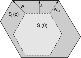
Figure 5:

and

$$O_{i}(\varepsilon)=(L_{i}(0))_{\varepsilon}\setminus(a_{i}(z)\cup b_{i}(z))$$

where $(A)_{\varepsilon}$ is the $\varepsilon$ - envelope of set $A$, i.e.

$$(A)_{\varepsilon}=\{x:dist(x,A)\leq\varepsilon\}.$$

The sets $a_{i}(z)$ and $b_{i}(z)$ are explained in Figure 6.

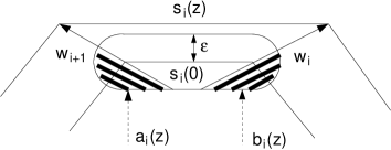
Figure 6:

Thus we have obtained a smooth vector field. Integrating this vector field we obtain the flow $\Upsilon^{t}(x_{1},x_{2},x_{3})$. We define transformation $\Psi$ as follows

$$\Psi(x_{1},x_{2},x_{3})=\left(\begin{array}[]{cc}\Upsilon^{1}(x_{1},x_{2},x_{3})\\ x_{3}\end{array}\right).$$

Finally our diffeomorphism has the form:

$$\Lambda(x_{1},x_{2},x_{3})=\left(\begin{array}[]{cc}\Upsilon^{1}(x_{1},x_{2},x_{3})\\ \Phi_{3}(x_{3})\end{array}\right),$$

where $\Phi_{3}$ is the third component of $\Phi$. ∎

From the proof of the above theorem we obtain the following

Corollary 1.

Let $J$ be the absolute value of Jacobian of transformation $\Lambda$, then:
a) $J\in L_{\infty}$,
b) if $|z_{i}|\leq M$, where $i=1,...,N+2$, then there exist $l,L$ such that $0<l\leq J\leq L$,
c) $\Lambda$ is a function of $(x_{1},x_{2},x_{3})$ and $z_{i}(t)$.

Now, we write the system (3) in the new variables. It is not hard to see that

$$\nabla_{(\tilde{x_{1}},\tilde{x_{2}},\tilde{x_{3}})}=\left(\nabla_{(x_{1},x_{2},x_{3})}\Lambda(x_{1},x_{2},x_{3},\tau)\right)^{-1}\nabla_{(x_{1},x_{2},x_{3})}$$

$$\frac{\partial}{\partial t}=\frac{\partial}{\partial\tau}-\left(\frac{\partial\Lambda}{\partial\tau}\right)^{T}\left(\nabla_{(x_{1},x_{2},x_{3})}\Lambda(x_{1},x_{2},x_{3},\tau)\right)^{-1}\nabla_{(x_{1},x_{2},x_{3})}$$

$$\nu=\frac{\left(\nabla_{(x_{1},x_{2},x_{3})}\Lambda(x_{1},x_{2},x_{3},\tau)\right)^{-1}\bf{n}}{\left|\left(\nabla_{(x_{1},x_{2},x_{3})}\Lambda(x_{1},x_{2},x_{3},\tau)\right)^{-1}\bf{n}\right|}.$$

We will use the following notation:

$$u(x_{1},x_{2},x_{3},\tau):=u(\tilde{x_{1}},\tilde{x_{2}},\tilde{x_{3}},t)|_{(\tilde{x_{1}},\tilde{x_{2}},\tilde{x_{3}},t)=(\Lambda(x_{1},x_{2},x_{3},\tau),\tau)}.$$

Let us denote by $H(t)$ the transformed Laplace operator and

$$\tilde{H}(t,z,\dot{z})\nabla_{(x_{1},x_{2},x_{3})}=\left(\left(\frac{\partial\Lambda}{\partial\tau}\right)^{T}+f\right)\left(\nabla_{(x_{1},x_{2},x_{3})}\Lambda(x_{1},x_{2},x_{3},\tau)\right)^{-1}\nabla_{(x_{1},x_{2},x_{3})}.$$

The boundary operator is defined as follows

$$B_{0}(t)\sigma=\frac{\left(\nabla_{(x_{1},x_{2},x_{3})}\Lambda(x_{1},x_{2},x_{3},\tau)\right)^{-1}\bf{n}}{\left|\left(\nabla_{(x_{1},x_{2},x_{3})}\Lambda(x_{1},x_{2},x_{3},\tau)\right)^{-1}\bf{n}\right|}\cdot\big{(}A(t),B(t),C(t)\big{)}\sigma$$

where $A,B$ and $C$ are defined in the following way

$$A(\tau)=\frac{1}{Q}\left(\Lambda^{2}_{x_{2}}\Lambda^{3}_{x_{3}}\partial_{x_{1}}-\Lambda^{2}_{x_{1}}\Lambda^{3}_{x_{3}}\partial_{x_{2}}\right),$$

$$B(\tau)=\frac{1}{Q}\left(\Lambda^{1}_{x_{1}}\Lambda^{3}_{x_{3}}\partial_{x_{2}}-\Lambda^{1}_{x_{2}}\Lambda^{3}_{x_{3}}\partial_{x_{1}}\right),$$

$$C(\tau)=\frac{1}{Q}\left(\left(\Lambda^{1}_{x_{2}}\Lambda^{2}_{x_{3}}-\Lambda^{1}_{x_{3}}\Lambda^{2}_{x_{2}}\right)\partial_{x_{1}}+\left(\Lambda^{1}_{x_{3}}\Lambda^{2}_{x_{1}}-\Lambda^{1}_{x_{1}}\Lambda^{2}_{x_{3}}\right)\partial_{x_{2}}+\left(\Lambda^{1}_{x_{1}}\Lambda^{2}_{x_{2}}-\Lambda^{1}_{x_{2}}\Lambda^{2}_{x_{1}}\right)\partial_{x_{3}}\right),$$

$$Q=\Lambda^{3}_{x_{3}}(\Lambda^{1}_{x_{1}}\Lambda^{2}_{x_{2}}-\Lambda^{1}_{x_{2}}\Lambda^{2}_{x_{1}}).$$

We have used the notation $\Lambda^{i}_{x_{j}}=\frac{\partial\Lambda^{i}}{\partial x_{j}}$. Finally, system (3) takes the form

$$\frac{\partial}{\partial t}u=H\big{(}z(t)\big{)}u+\tilde{H}\big{(}z(t),\dot{z}(t)\big{)}\nabla u+\left(H(t)+\tilde{H}(t)\nabla-\frac{\partial}{\partial t}\right)G\text{ in }\Omega_{0}^{c},$$

$$B_{0}(t)u=0\text{ on }\partial\Omega_{0}^{c},$$ (13)

$$\frac{1}{\mathcal{H}^{2}(S_{i}(t))}\int_{S_{i}(0)}\big{(}u(x)+G\big{)}J\big{(}x,z(t)\big{)}\,d\mathcal{H}^{2}(x)=\kappa_{i}(t)+\beta_{i}V_{i},$$

$$u(0)=u_{0},\,z(0)=0.$$

where $f,G,u$ are old $f,G,u$ in new variables.

4 The existence of a solution - a linear theory

In this section we show solvability of the following problem

$$\frac{\partial}{\partial t}u=H(t)u-\delta u+f(t)\text{ in }\Omega_{0}^{c},$$

$$B_{0}(t)u=0\text{ on }\partial\Omega_{0}^{c},$$

$$u(0)=u_{0},$$

where $\delta$ will be specified later and $f$ is a Hölder continuous map.
Let us define an operator with the domain

$$H(t):D\big{(}H(t),\Omega^{c}\big{)}\rightarrow L^{2}(\Omega^{c})$$

$$D\big{(}H(t),\Omega^{c}\big{)}:=\left\{v\in H^{1}(\Omega^{c}):H(t)v\in L^{2}(\Omega^{c}),B_{0}(t)v|_{\partial\Omega^{c}}=0\right\}.$$

Where the norm is defined as follows

$$||u||_{D(H(t),\Omega^{c})}:=\left(||u||^{2}_{H^{1}(\Omega^{c})}+||H(t)u||^{2}_{L^{2}(\Omega^{c})}\right)^{\frac{1}{2}}.$$

Later we will need the following

Proposition 1.

$D(H(t),\Omega^{c})$ is Banach space for each $t\geq 0$.

Proof.

We know that $D(H(t),\Omega^{c})$ and $D(\Delta,\Omega^{c}(t))$ are isomorphic (see the proof of Corollary 3). Hence, it is enough to show that $D(\Delta,\Omega^{c}(t))$ is Banach space.

Let us take Cauchy sequence $\{u_{k}\}$ from $D(\Delta,\Omega^{c}(t))$. Subsequently, $D_{x_{i}}u_{k}$ and $\Delta u_{k}$ are Cauchy sequences in $L^{2}(\Omega^{c}(t))$. So $D_{x_{i}}u_{k}\rightarrow v_{i}$ and $\Delta u_{k}\rightarrow f$ in $L^{2}(\Omega^{c}(t))$. In particular $u_{k}\rightarrow u$ in $L^{2}(\Omega^{c}(t))$. Hence,

$$\int_{\Omega^{c}(t)}uD_{x_{i}}\phi dx\leftarrow\int_{\Omega^{c}(t)}u_{k}D_{x_{i}}\phi dx=(-1)\int_{\Omega^{c}(t)}D_{x_{i}}u_{k}\phi dx\rightarrow(-1)\int_{\Omega^{c}(t)}v_{i}\phi dx.$$

Analogously

$$\int_{\Omega^{c}(t)}u\Delta\phi dx\leftarrow\int_{\Omega^{c}(t)}u_{k}\Delta\phi dx=(-1)^{2}\int_{\Omega^{c}(t)}\Delta u_{k}\phi dx\rightarrow(-1)^{2}\int_{\Omega^{c}(t)}f\phi dx.$$

Hence, we obtain $D_{x_{i}}u=v_{i}$ and $\Delta u=f$. From trace theorem and $D(\Delta,\Omega^{c}(t))\subset H^{\frac{3}{2}+\varepsilon}(\Omega^{c}(t))$ (see [16]) we obtain

$$\left|\left|\frac{\partial(u_{l}-u_{k})}{\partial\nu}\right|\right|_{L^{2}(\partial\Omega^{c}(t))}\leq C||u_{l}-u_{k}||_{D(\Delta,\Omega^{c}(t))}.$$

Hence, we obtain the assertion of the proposition. ∎

Now, we show the following

Lemma 4.

If $u\in D(\Delta,\Omega)$ then there exists a sequence $\{R_{n}\}$, $R_{n}\rightarrow\infty$ such that

$$\lim_{R_{n}\rightarrow\infty}\int_{\partial B(0,R_{n})}\frac{\partial u}{\partial\nu}\bar{u}\,d\mathcal{H}^{2}=0$$

Proof.

From the integration by parts formula the following expression follows

$$\int_{\Omega^{c}\setminus B(0,R)}u\Delta udx+\int_{\Omega^{c}\setminus B(0,R)}|\nabla u|^{2}dx=\int_{\partial B(0,R)}\frac{\partial u}{\partial\nu}\bar{u}\,d\mathcal{H}^{2}.$$

But $u,\nabla u,\Delta u\in L^{2}(\Omega^{c})$. Hence there exists a sequence $R_{n}$ such that

$$\int_{\Omega^{c}\setminus B(0,R_{n})}u\Delta udx\rightarrow 0,$$

$$\int_{\Omega^{c}\setminus B(0,R_{n})}|\nabla u|^{2}dx\rightarrow 0$$

as $R_{n}\rightarrow\infty$.
From this the lemma follows. ∎

Now, we can go to the following result.

Theorem 3.

Each of the operators $-H(t)$, $t\geq 0$, generates an analytic semigroup.

Proof.

It is enough to show that $-H(t)$ is a sectorial operator (see [23] or [20]). First of all we examine the operator $H(0)$, i.e. $\Delta$. Namely, we show the following,

Lemma 5.

The operator $-\Delta$ with the domain $D(\Delta,\Omega^{c})$ is sectorial in $L^{2}(\Omega^{c})$.

Proof.

First of all we show that the operator $-\Delta$ is closed and densely defined. Indeed, since $C^{\infty}_{0}(\Omega)\subset D(\Delta,\Omega)$ and $C^{\infty}_{0}(\Omega)$ is dense in $L^{2}(\Omega)$, hence $D(\Delta,\Omega)$ is dense in $L^{2}(\Omega)$. Now, we show that $-\Delta$ is a closed operator.

We need the following estimate

$$||\nabla v||^{2}_{L^{2}(\Omega^{c})}\leq||v||_{L^{2}(\Omega^{c})}||\Delta v||_{L^{2}(\Omega^{c})}$$ (14)

for $v\in D(\Delta,\Omega^{c})$. In order to show inequality (14) we take the following equality

$$\Delta v=f$$

where $f\in L^{2}(\Omega^{c})$ and $v\in D(\Delta)$. We multiply both sides of the above equality by $v$ and after integration by parts we get,

$$||\nabla v||^{2}_{L^{2}(\Omega^{c})}=\int_{\Omega^{c}}vfdx\leq||v||_{L^{2}(\Omega^{c})}||f||_{L^{2}(\Omega^{c})}=||v||_{L^{2}(\Omega^{c})}||\Delta v||_{L^{2}(\Omega^{c})},$$

where we used Lemma 4 and Schwarz inequality.

Now, let us take a sequence $\{v_{k}\}_{k=1}^{\infty}\subset D(\Delta,\Omega^{c})$ such that:

$$v_{k}\rightarrow v$$

$$\Delta v_{k}\rightarrow f$$

in $L^{2}(\Omega^{c})$. From inequality (14) we obtain

$$||v_{k}-v_{l}||^{2}_{D(\Delta,\Omega^{c})}=||v_{k}-v_{l}||^{2}_{H^{1}(\Omega^{c})}+||\Delta v_{k}-\Delta v_{l}||^{2}_{L^{2}(\Omega^{c})}=$$

$$||v_{k}-v_{l}||^{2}_{L^{2}(\Omega^{c})}+||\nabla v_{k}-\nabla v_{l}||^{2}_{L^{2}(\Omega^{c})}+||\Delta v_{k}-\Delta v_{l}||^{2}_{L^{2}(\Omega^{c})}\leq$$

$$||v_{k}-v_{l}||^{2}_{L^{2}(\Omega^{c})}+||v_{k}-v_{l}||_{L^{2}(\Omega^{c})}||\Delta v_{k}-\Delta v_{l}||_{L^{2}(\Omega^{c})}+||\Delta v_{k}-\Delta v_{l}||^{2}_{L^{2}(\Omega^{c})}\leq$$

$$\left(||v_{k}-v_{l}||_{L^{2}(\Omega^{c})}+||\Delta v_{k}-\Delta v_{l}||_{L^{2}(\Omega^{c})}\right)^{2}.$$

Hence

$$||v_{k}-v_{l}||_{D(\Delta,\Omega^{c})}\leq||v_{k}-v_{l}||_{L^{2}(\Omega^{c})}+||\Delta v_{k}-\Delta v_{l}||_{L^{2}(\Omega^{c})}.$$

Subsequently, we obtain that $\{v_{k}\}_{k=1}^{\infty}$ is Cauchy sequence in $D(\Delta,\Omega^{c})$. Finally,

$$v_{k}\rightarrow v\text{ w }D(\Delta,\Omega^{c}).$$

Hence, $v\in D(\Delta,\Omega^{c})$ and $\Delta v_{k}\rightarrow\Delta v$.

Now, we show the estimate for a resolvent operator. We follow the method used in the book [20]. Let us consider the equation

$$\lambda u+\Delta u=f$$

where $f\in L^{2}$ and $u\in D(\Delta)$. Let us assume that $Re\lambda<0$.
Let us multiply the above equation by $\bar{u}$ and integrate:

$$\int_{\Omega^{c}}\lambda|u|^{2}+\bar{u}\Delta u=\int_{\Omega^{c}}\bar{u}f.$$

Integrating by parts we obtain

$$\int_{\Omega^{c}}\lambda|u|^{2}-|\nabla u|^{2}=\int_{\Omega^{c}}\bar{u}f,$$

where we applied Lemma 4.

Next, we take the real and imaginary part of above expression:

$$Re\lambda||u||^{2}_{L^{2}}-||\nabla u||^{2}_{L^{2}}=Re\int_{\Omega^{c}}\bar{u}f$$

$$-Im\lambda||u||^{2}_{L^{2}}=Im\int_{\Omega^{c}}\bar{u}f.$$

Hence,

$$Re\lambda||u||_{L^{2}(\Omega^{c})}\leq||f||_{L^{2}(\Omega^{c})}$$

$$|Im\lambda|\,||u||_{L^{2}(\Omega^{c})}\leq||f||_{L^{2}(\Omega^{c})}.$$

Subsequently, we take a sum of the above inequalities

$$|\lambda|\,||u||_{L^{2}(\Omega^{c})}\leq 2||f||_{L^{2}(\Omega^{c})}.$$

Next, for arbitrary $\lambda$ we behave in a standard way. It means, if $Re\lambda>0$ and $\phi\leq|\arg(\lambda)|\leq\pi$, let us denote $\lambda=a+ib$ we obtain $\tan\phi\leq\left|\frac{b}{a}\right|$. From the above estimates we obtain:

$$|b|\,||u||_{L^{2}(\Omega^{c})}\leq||f||_{L^{2}(\Omega^{c})}$$

and

$$|a|\,||u||_{L^{2}}\leq\frac{||f||_{L^{2}}}{tg\phi}.$$

Hence,

$$|\lambda|\,||u||_{L^{2}(\Omega^{c})}\leq\frac{1}{|\sin\phi|}||f||_{L^{2}(\Omega^{c})}.$$

This ends the proof of the lemma. ∎

Now, we show Theorem 3 for arbitrary $t>0$.

Using the same argument as proof of Lemma 5 one can show $-H(t)$ is densely defined. Subsequently, we show that the operator $-H(t)$ is closed. First of all we show the following inequalities

$$||\nabla u||^{2}_{L^{2}(\Omega^{c})}\leq c||H(t)u||_{L^{2}(\Omega^{c})}\,||u||_{L^{2}(\Omega^{c})},$$ (15)

where $u\in D(H(t),\Omega^{c})$. Indeed, let us consider the equation

$$H(t)u=f\text{ in }\Omega^{c}.$$

Changing the variables in the above equation we obtain the following one

$$\Delta u=f\text{ in }\Omega^{c}(t).$$

where $u$ and $f$ are old $u$ and $f$ in the new variables. Following the method presented in the proof of Lemma 5 and from Corollary 1 we obtain the inequality (15).

From inequality (15) closedness easily follows. Indeed, let us take any sequence $\{u_{k}\}\subset D(H(t),\Omega)$ such that $u_{k}\rightarrow u$ and $H(t)u_{k}\rightarrow f$ in $L^{2}(\Omega)$. Hence $u_{k}$ and $H(t)u_{k}$ are Cauchy sequences in $L^{2}(\Omega)$. Subsequently, from inequality (15) we obtain the following estimate

$$||\nabla u_{k}-\nabla u_{l}||^{2}_{L^{2}(\Omega^{c})}\leq c||H(t)(u_{k}-u_{l})||_{L^{2}(\Omega^{c})}\,||u_{k}-u_{l}||_{L^{2}(\Omega^{c})}$$

and this inequality finishes the closedness of the operator $H(t)$ (see proof the Lemma 5 for details).

Now, we show the estimate for the resolvent operator. Let us consider the equation

$$\lambda u+H(t)u=f\text{ in }\Omega^{c}.$$

where $f\in L^{2}$ and $u\in D(H(t),\Omega^{c})$. Changing the variables in the above equation we obtain the following equation

$$\lambda u+\Delta u=f\text{ in }\Omega^{c}(t),$$

where $u$ and $f$ are old $u$ and $f$ in the new variables.

From the proof of the Lemma 5 we obtain the inequality

$$|\lambda|\,||u||_{L^{2}(\Omega^{c}_{t})}\leq C||f||_{L^{2}(\Omega^{c}_{t})}.$$

After changing the variables we obtain

$$|\lambda|\int_{\Omega^{c}}|u|^{2}Jdx\leq C\int_{\Omega^{c}}|f|^{2}Jdx.$$

From Corollary 1 the following

$$|\lambda|\,||u||_{L^{2}(\Omega^{c})}\leq C\frac{L}{l}||f||_{L^{2}(\Omega^{c})}$$

holds.

From this the theorem follows. ∎

Before we state next result we recall the definition of some hypothesis (see [1] and [2]). Namely,

Hypothesis I. For each $t\in[0,T]$, $A(t):D(A(t))\subseteq L^{2}\rightarrow L^{2}$ is a closed linear operator and there exist $M>0$ and $\theta_{0}\in(\frac{\pi}{2},\pi]$ such that

$$\rho(A(t))\supseteq S_{\theta_{0}}=\{z\in\mathbb{C}:|\arg z|\leq\theta_{0}\}\text{ }\forall t\in[0,T],$$

$$||R(\lambda,A(t))||_{{\cal{L}}(L^{2})}\leq\frac{M}{1+|\lambda|}\text{ }\forall\lambda\in S_{\theta_{0}},\forall t\in[0,T].$$

Hypothesis II. There exist $B>0$, $k\in\mathbb{N}$, $\alpha_{1},...,\alpha_{k},\beta_{1},...,\beta_{k}$ with $0\leq\beta_{i}<\alpha_{i}\leq 2$, such that

$$||A(t)R(\lambda,A(t))[A(t)^{-1}-A(s)^{-1}]||_{{\cal{L}}(L^{2})}\leq B\sum_{i=1}^{k}(t-s)^{\alpha_{i}}|\lambda|^{\beta_{i}-1}\text{ }$$

$\forall\lambda\in S_{\theta_{0}}\setminus\{0\}$, $\forall 0\leq s\leq t\leq T$. Where $R(\lambda,A(t))$ is resolvent operator.

We have the following

Theorem 4.

There exists $\delta>0$ such that the operator

$$A(t)=H(t)-\delta Id$$

with a domain $D(A(t))=D(H(t))$ fulfills Hypothesis I and Hypothesis II.

Proof.

The proof of Hypothesis I is almost the same as the proof of Theorem 3.

Concerning Hypothesis II, if we set for$f\in L^{2}(\Omega^{c})$

$$v=A(s)^{-1}f,\text{ }u=R\big{(}\lambda,A(t)\big{)}\big{[}\lambda-A(s)\big{]}v,$$

then we have to estimate $L^{2}$-norm of

$$u-v=A(t)R\big{(}\lambda,A(t)\big{)}\left[A(t)^{-1}-A(s)^{-1}\right]f.$$

Now, $u$ and $v$ solve respectively,

$$\lambda u-A(t)u=\lambda v-f\text{ in }\Omega^{c}$$

$$B(t)u=0\text{ on }\partial\Omega^{c}$$

and

$$A(s)v=-f\text{ in }\Omega^{c}$$

$$B(s)v=0\text{ on }\partial\Omega^{c}.$$

Hence, $u-v$ solves

$$\lambda(u-v)+A(s)v-A(t)u=0\text{ in }\Omega^{c}$$

$$B(t)u=B(s)v\text{ on }\partial\Omega^{c}.$$

Next, using the similar methods as in the proof of Theorem 3 and from inequality

$$||\nabla v||_{L^{2}(\Omega^{c})}\leq c||f||_{L^{2}(\Omega^{c})}$$

and Lipschitz continuity of coefficients of the operator $A$ the proof follows. ∎

Now, from the above theorem and [1] the following holds.

Corollary 2.

If $f$ is a Hölder continuous map, then there exists unique solution of the following problem

$$\frac{\partial}{\partial t}u=A(t)u+f(t)\text{ on }\Omega_{0}^{c},$$

$$B_{0}(t)u=0\text{ in }\partial\Omega_{0}^{c},$$

$$u(0)=u_{0}.$$

It is given by the formula

$$u(t)=U(t,0)u_{0}+\int_{0}^{t}U(t,\sigma)f(\sigma)d\sigma.$$

5 Nonlinear theory

Before we state the main result we are going to present some facts.

In order to understand better interpolation spaces we show isomorphism theorem.

Corollary 3.

The following interpolation spaces are isomorphic

$$\left[L^{2}(\Omega^{c}_{t}),D(\Delta,\Omega^{c}_{t})\right]_{\theta}\backsimeq\left[L^{2}(\Omega^{c}),D(H(t),\Omega^{c})\right]_{\theta}.$$

Proof.

From Theorem 2 we know that there is a family of $C^{2+\alpha}$ diffeomorphisms $\Lambda_{t}:\Omega^{c}_{t}\rightarrow\Omega^{c}$. Let us denote by $\Lambda_{t_{*}}$ the pullback operator. Hence we can write the following diagram

So we obtain an isomorphism on the level of interpolation pairs. It is well known (see [33]) that interpolation is a functor from a category of Banach pairs into a category of interpolation spaces. Hence, from functoriality (see [30] or [24]) we obtain

Where $\theta$ is the interpolation functor. ∎

Corollary 4.

If $\beta>\frac{s}{\frac{3}{2}+\epsilon}$, $\epsilon$ is sufficiently small and $s<\frac{3}{2}+\epsilon$, then the following is true

$$\left[L^{2}(\Omega^{c}),D(H(t),\Omega^{c})\right]_{\beta}\hookrightarrow H^{s}(\Omega^{c}).$$

Proof.

It follows immediately from the properties of interpolation spaces and Grisvard theory (see [16] and [17]), see also [33]. ∎

Now, we show a compactness result.

Lemma 6.

Let us assume $\Omega\subset\mathbb{R}^{k}$ is bounded domain with Lipschitz boundary. Let us also assume that the sequence ${u_{n}}$ is bounded in $H^{\sigma}(\mathbb{R}^{k}\setminus\Omega)$ and $||u_{n}||_{H^{\sigma}(\mathbb{R}^{k}\setminus B(0,N))}\rightarrow 0$ as $N\rightarrow\infty$ uniformly with respect to $n$. Then there exists subsequence of $u_{n}$ convergence in $H^{\alpha}(\mathbb{R}^{k}\setminus\Omega)$ for $\alpha<\sigma$.

Proof.

We can assume that $\Omega\subset B(0,1)$. Let $\{u_{n}\}\subset H^{\sigma}(\mathbb{R}^{k}\setminus\Omega)$, then $\{u_{n}|_{B(0,N)}\}\subset H^{\sigma}(B(0,N)\setminus\Omega)$. Using Rellich - Kondrachov Theorem we can extract a sequence $\{u_{n_{1}}|_{B(0,1)}\}\subset H^{\sigma}(B(0,1)\cap\Omega)$ such that $\{u_{n_{1}}|_{B(0,1)}\}\rightarrow u_{1}$ in $H^{\alpha}(B(0,1)\setminus\Omega)$. Let us denote by $\tilde{u}_{1}$ extension of $u_{1}$ onto $\mathbb{R}^{k}\setminus\Omega$. So we have chosen a subsequence $\{u_{n_{1}}\}$ (we restrict the sequence to such that the following inequality is satisfied $||u_{n_{1}}-\tilde{u}_{1}||_{H^{\alpha}(B(0,1)\setminus\Omega)}\leq 1$). Analogously we work on ball $B(0,2)$, e.g. we subtract subsequence $\{u_{n_{1}}|_{B(0,2)}\}$, (we will denote it by $\{u_{n_{2}}|_{B(0,2)}\}$) such that $\{u_{n_{2}}|_{B(0,2)}\}\rightarrow u_{2}$. Denote extension by $\tilde{u}_{2}$ and we take only this terms such $||u_{n_{2}}-\tilde{u}_{2}||_{H^{\alpha}(B(0,2)\setminus\Omega)}\leq\frac{1}{2}$ end so on, namely
$u_{n_{1}}\rightarrow u_{1}$ in $H^{\alpha}(B(0,1)\setminus\Omega)$ and extension $\tilde{u}_{1}$
and such that $||u_{n_{1}}-\tilde{u}_{1}||_{H^{\alpha}(B(0,1)\setminus\Omega)}\leq 1$
$u_{n_{2}}\rightarrow u_{2}$ in $H^{\alpha}(B(0,2)\setminus\Omega)$ and extension $\tilde{u}_{2}$
and such that $||u_{n_{2}}-\tilde{u}_{2}||_{H^{\alpha}(B(0,2)\setminus\Omega)}\leq\frac{1}{2}$
$u_{n_{3}}\rightarrow u_{3}$ in $H^{\alpha}(B(0,3)\setminus\Omega)$ and extension $\tilde{u}_{3}$
and such that $||u_{n_{3}}-\tilde{u}_{3}||_{H^{\alpha}(B(0,3)\setminus\Omega)}\leq\frac{1}{3}$
.
.
.
$u_{n_{N}}\rightarrow u_{N}$ in $H^{\alpha}(B(0,N)\setminus\Omega)$ and extension $\tilde{u}_{N}$
and such that $||u_{n_{N}}-u_{N}||_{H^{\alpha}(B(0,N)\setminus\Omega)}\leq\frac{1}{N}$
where $u_{n_{N}}$ is subsequence of $u_{n_{M}}$ for $N>M$. We shall show that $\{\tilde{u}_{N}\}$ is convergent in $H^{\alpha}(\mathbb{R}^{k}\setminus\Omega)$. Indeed, we show that Cauchy condition is fulfilled

$$||\tilde{u}_{N}-\tilde{u}_{M}||_{H^{\alpha}(\mathbb{R}^{k}\setminus\Omega)}\leq||\tilde{u}_{N}-\tilde{u}_{M}||_{H^{\alpha}(\Omega\cap B(0,min\{N,M\})}+$$

$$||\tilde{u}_{N}||_{H^{\alpha}(\mathbb{R}^{k}\setminus B(0,min\{N,M\}))}+||\tilde{u}_{M}||_{H^{\alpha}(\mathbb{R}^{k}\setminus B(0,min\{N,M\}))}.$$

Hence, we obtain

$$\underset{N,M\rightarrow\infty}{\lim\sup}||\tilde{u}_{N}-\tilde{u}_{M}||_{H^{\alpha}(\mathbb{R}^{k}\setminus\Omega)}=0.$$

Let us denote the limit of this sequence by $u$. We show that $u_{n_{N}}$ converges to $u$ in $H^{\alpha}(\mathbb{R}^{k}\setminus\Omega)$. Namely,

$$||u_{n_{N}}-u||_{H^{\alpha}(\mathbb{R}^{k}\setminus\Omega)}\leq||u_{n_{N}}-u||_{H^{\alpha}(B(0,N)\setminus\Omega)}+$$

$$||u_{n_{N}}||_{H^{\alpha}(\mathbb{R}^{k}\setminus B(0,N))}+||u||_{H^{\alpha}(\mathbb{R}^{k}\setminus B(0,N))}.$$

These last two terms converge to $0$, and

$$||u_{n_{N}}-u||_{H^{\alpha}(B(0,N)\setminus\Omega)}\leq||u_{n_{N}}-\tilde{u}_{N}||_{H^{\alpha}(B(0,N)\setminus\Omega)}+||\tilde{u}_{N}-u||_{H^{\alpha}(B(0,N)\setminus\Omega)}$$

$$\leq\frac{1}{N}+||\tilde{u}_{N}-u||_{H^{\alpha}(\mathbb{R}^{3}\setminus\Omega)}.$$

This finishes the proof. ∎

Now, we can formulate the main result.

Theorem 5.

Let us assume $u_{0}\in D(A(0))$ and $g\in C^{1,\eta}((0,T);\mathbb{R}^{N+2})$, then there exists a solution of the problem

$$\frac{\partial u}{\partial t}=H\big{(}z(t)\big{)}u+\tilde{H}\big{(}z(t),\dot{z}(t)\big{)}\nabla u+\left(H(t)+\tilde{H}(t)\nabla-\frac{\partial}{\partial t}\right)G,$$

$$B_{0}(t)u=0,$$

$$\dot{z}_{i}=-\frac{1}{\beta_{i}}\kappa_{i}\big{(}z(t)\big{)}+\frac{1}{\beta_{i}\mathcal{H}^{2}(S_{i}(z))}\int_{S_{i}(0)}\big{(}u(x)+G\big{)}J\big{(}x,z(t)\big{)}d\mathcal{H}^{2}(x),$$

$$u(0)=u_{0},z(0)=0.$$

such that $u\in C^{\alpha}([0,T);H^{s}(\Omega^{c}))$ and $z\in(C^{1,\alpha}([0,T)))^{N+2}$. Where $1<s<\frac{3}{2}+\epsilon$ and $\alpha<min(1-(\frac{3}{2}+\epsilon)^{-1}s,\eta)$.

For the sake of simplicity of notation we shall write $L^{2}=L^{2}(\Omega^{c})$ and $H^{s}=H^{s}(\Omega^{c})$.

Proof.

We will apply the method of successive approximation. We set

$$u^{0}(t)=u_{0},\text{ }t\in[0,\infty)$$

and let $z_{i}^{0}$ be a solution of the following problem

$$\frac{d}{dt}{z_{i}}^{0}=\frac{1}{\beta_{i}}\kappa_{i}\big{(}z^{0}(t)\big{)}+\frac{1}{\beta_{i}\mathcal{H}^{2}(S_{i}(z))}\int_{S_{i}(0)}\big{(}u^{0}(x)+G\big{)}J\big{(}x,z(t)\big{)}d\mathcal{H}^{2}(x),$$

$$z_{i}^{0}=0,$$

on the maximal interval of existence $[0,T_{0})$. Next, we define $u^{n+1}$ as an unique solution (on interval  $[0,T_{n})$) of the following problem

$$\frac{\partial u^{n+1}}{\partial t}=H(t)u^{n+1}+\tilde{H}(t)\nabla u^{n+1}+\left(H(t)+\tilde{H}(t)\nabla-\frac{\partial}{\partial t}\right)G$$

$$B_{0}u^{n+1}=0$$ (16)

$$u^{n+1}(0)=u_{0}.$$

Subsequently, we define $z_{i}^{n+1}$ as a unique solution of

$$\frac{d}{dt}{z_{i}}^{n+1}=\frac{1}{\beta_{i}}\kappa_{i}\big{(}z^{n+1}(t)\big{)}+\frac{1}{\beta_{i}\mathcal{H}^{2}(S_{i}(z))}\int_{S_{i}(0)}\big{(}u^{n+1}(x)+G\big{)}J\big{(}x,z^{n+1}(t)\big{)}d\mathcal{H}^{2}(x),$$ (17)

$$z_{i}^{n+1}=0$$

on the maximal interval of existence $[0,T_{n+1})$, where $T_{n+1}\leq T_{n}$.

We shall show that sequences $u^{n}$ and $z^{n}$ are equibounded and equicontinuous.

We can solve the parabolic equation (5) using methods from previous section. Let as denote $H(t)=H(z(t))$ and $\tilde{H}(t)=\tilde{H}(z(t),\dot{z}(t))$.

We will show that the equation (5) has a unique solution. Indeed, let us denote by ${\cal T}$ an operator defined as follows

$${\cal T}w(t)=U(t,0)u_{0}+\int_{0}^{t}U(t,\sigma)\left(\delta w(\sigma)+\tilde{H}(\sigma)\nabla w(\sigma)+\left(H(\sigma)+\tilde{H}(\sigma)\nabla-\frac{\partial}{\partial\sigma}\right)G\right)d\sigma.$$

We will show that the operator ${\cal T}$ possesses exactly one fixed point. First of all we shall show that there exist $T_{n}>0$ and $\varepsilon_{n}>0$ such that

$$B(u_{0},\varepsilon_{n})\subset C([0,T_{n}];H^{s})$$

$${\cal T}:B(u_{0},\varepsilon_{n})\rightarrow B(u_{0},\varepsilon_{n}).$$

Let us notice

$$\sup_{s\in[0,T_{n-1}]}||\tilde{H}(s)||_{L_{\infty}(\Omega^{c})}\leq$$

$$\sup_{(z,v)\in B(\varepsilon_{0})\times B(\varepsilon_{0}^{\prime})}\left|\left|\left(\frac{\partial\Lambda}{\partial s}\right)^{T}\left(\nabla_{(x_{1},x_{2},x_{3})}\Lambda(x_{1},x_{2},x_{3},s)\right)^{-1}\right|\right|_{L_{\infty}(\Omega^{c})}+$$

$$+\sup_{s\in[0,T_{1}]}\left|\left|f\left(\nabla_{(x_{1},x_{2},x_{3})}\Lambda(x_{1},x_{2},x_{3},s)\right)^{-1}\right|\right|_{L_{\infty}(\mathbb{R}^{3}\times\mathbb{R}_{+})}\leq M_{1},$$

where $B(\varepsilon_{0})$ and $B(\varepsilon_{0}^{\prime})$ are balls in $C^{1}$ and $C^{\alpha}$ respectively, such that the solution $z_{i}^{0}$ is contained in $B(\varepsilon_{0})$ and $\dot{z}_{i}^{0}$ in $B(\varepsilon_{0}^{\prime})$.

Since $G$ has a compact support it is not hard to see that

$$\sup_{s\in[0,T_{n-1}]}\left|\left|\left(H(\sigma)+\tilde{H}(\sigma)\nabla-\frac{\partial}{\partial\sigma}\right)G\right|\right|_{L_{2}(\Omega^{c})}\leq M_{2}.$$

Using the above inequalities and Corollary 4 we can write

$$\big{|}\big{|}{\cal T}w(t)-u_{0}\big{|}\big{|}_{H^{s}}\leq c\int_{0}^{t}\big{|}\big{|}A(\sigma)U(\sigma,0)u_{0}\big{|}\big{|}_{\left[D(A(\sigma)),L_{2}\right]_{\beta}}d\sigma+c\int_{0}^{t}\big{|}\big{|}U(t,\sigma)\delta w(\sigma)\big{|}\big{|}_{\left[D(A(t)),L_{2}\right]_{\beta}}d\sigma+$$

$$c\int_{0}^{t}\big{|}\big{|}U(t,\sigma)\tilde{H}(\sigma)\nabla w(\sigma)\big{|}\big{|}_{[D(A(t)),L_{2}]_{\beta}}d\sigma+c\int_{0}^{t}\left|\left|U(t,\sigma)\left(H(\sigma)+\tilde{H}(\sigma)\nabla-\frac{\partial}{\partial\sigma}\right)G\right|\right|_{[D(A(t)),L_{2}]_{\beta}}d\sigma.$$

Using the methods from [23] one can show that the following inequalities

$$\big{|}\big{|}A(t)U(t,\sigma)u\big{|}\big{|}_{\left[D(A(t)),L_{2}\right]_{\beta}}\leq\frac{c}{(t-\sigma)^{1+\beta-\theta}}\big{|}\big{|}u\big{|}\big{|}_{\left[D(A(\sigma)),L_{2}\right]_{\theta}},$$

$$\left|\left|U(t,\sigma)u\right|\right|_{[D(A(t)),L_{2}]_{\beta}}\leq\frac{c}{(t-\sigma)^{\beta}}\left|\left|u\right|\right|_{L_{2}}$$

hold for $u\in D(A(\sigma))$. Next, we obtain

$$\big{|}\big{|}{\cal T}w(t)-u_{0}\big{|}\big{|}_{H^{s}}\leq c\int_{0}^{t}\frac{1}{\sigma^{1+\beta-\theta}}\big{|}\big{|}u_{0}\big{|}\big{|}_{[D(A(0)),L_{2}]_{\theta}}d\sigma+c\delta\int_{0}^{t}\frac{1}{(t-\sigma)^{\beta}}\big{|}\big{|}w(\sigma)\big{|}\big{|}_{L_{2}}d\sigma+$$

$$c\int_{0}^{t}\frac{1}{(t-\sigma)^{\beta}}\big{|}\big{|}\tilde{H}(\sigma)\nabla w(\sigma)\big{|}\big{|}_{L_{2}}d\sigma+c\int_{0}^{t}\frac{1}{(t-\sigma)^{\beta}}\left|\left|\left(H(\sigma)+\tilde{H}(\sigma)\nabla-\frac{\partial}{\partial\sigma}\right)G\right|\right|_{L_{2}}d\sigma\leq$$

$$cT_{n}^{\theta-\beta}||u_{0}||_{[D(A(0)),L_{2}]_{\theta}}+cT_{n}^{1-\beta}\left((\delta+M_{1})\sup_{\sigma\in[0,T_{n}]}||w(\sigma)||_{H^{s}}+M_{2}\right),$$

where $\theta>\beta$. But $w\in B(u_{0},\varepsilon_{n})$, hence, we choose $T_{n}$ and $\varepsilon_{n}$ such that

$$\sup_{t\in[0,T_{n}]}\big{|}\big{|}{\cal T}w(t)-u_{0}\big{|}\big{|}_{H^{s}}\leq cT_{n}^{\theta-\beta}\big{|}\big{|}u_{0}\big{|}\big{|}_{[D(A(0)),L_{2}]_{\theta}}+$$ (18)

$$cT_{n}^{1-\beta}\left((\delta+M_{1})\big{|}\big{|}w(\sigma)\big{|}\big{|}_{H^{s}}+M_{2}\right)+\varepsilon_{n}T_{n}^{1-\beta}(c\delta+M_{1}c)\leq\varepsilon_{n}.$$

Now, we show that the operator ${\cal T}$ is a contraction. Indeed,

$$\big{|}\big{|}{\cal T}u(t)-{\cal T}v(t)\big{|}\big{|}_{H^{s}}\leq c\delta\int_{0}^{t}\left|\left|U(t,\sigma)\big{(}u(\sigma)-v(\sigma)\big{)}\right|\right|_{[D(A(t)),L_{2}]_{\beta}}d\sigma+$$

$$c\int_{0}^{t}\big{|}\big{|}U(t,\sigma)\tilde{H}(\sigma)\big{(}\nabla u(\sigma)-\nabla v(\sigma)\big{)}\big{|}\big{|}_{[D(A(t)),L_{2}]_{\beta}}d\sigma\leq c\delta\int_{0}^{t}\frac{1}{(t-\sigma)^{\beta}}\big{|}\big{|}u(\sigma)-v(\sigma)\big{|}\big{|}_{L_{2}}d\sigma+$$

$$c\int_{0}^{t}\frac{1}{(t-\sigma)^{\beta}}\big{|}\big{|}\tilde{H}(\sigma)\big{(}\nabla u(\sigma)-\nabla v(\sigma)\big{)}\big{|}\big{|}_{{L^{2}}}d\sigma\leq(c\delta+cM_{1})T_{n}^{1-\beta}\sup_{\sigma\in[0,T_{n}]}\big{|}\big{|}u(\sigma)-v(\sigma)\big{|}\big{|}_{H^{s}}.$$

We find $\varepsilon_{n}$ and $T_{n}$ such that ${\cal T}$ is a contraction and the inequality (18) is satisfied. Hence, from Banach fixed point theorem we obtain that ${\cal T}$ has a unique fixed point. Let us notice that $\varepsilon_{n}=\varepsilon_{2}$ and $T_{n}=T_{2}$ for $n\geq 2$.

We will show the following

Lemma 7.

The sequence $u^{n}$ is equibounded and equicontinuous on $[0,T_{2}]$.

Proof.

Equiboundedness follows from previous considerations and construction of the sequence $u^{n}$. Let us denote by $a$ an upper bound of $u^{n}$, i.e.

$$\sup_{\sigma\in[0,T_{2}]}||u^{n}(\sigma)||_{H^{s}}\leq a.$$

Now, we show that the sequence $u^{n}$ is equicontinuous. Namely,

$$||u^{n+1}(t)-u^{n+1}(\tau)||_{H^{s}}\leq||U(t,0,)u_{0}-U(\tau,0)u_{0}||_{H^{s}}+$$

$$+\int_{0}^{t}\left|\left|\big{(}U(t,\sigma)-U(\tau,\sigma)\big{)}\left(\delta u^{n+1}(\sigma)+\tilde{H}(\sigma)\nabla u^{n+1}(\sigma)+\left(H(\sigma)+\tilde{H}(\sigma)\nabla-\frac{\partial}{\partial\sigma}\right)G\right)\right|\right|_{H^{s}}d\sigma+$$

$$+\int_{\tau}^{t}\left|\left|U(t,\sigma)\left(\delta u^{n+1}(\sigma)+\tilde{H}(\sigma)\nabla u^{n+1}(\sigma)+\left(H(\sigma)+\tilde{H}(\sigma)\nabla-\frac{\partial}{\partial\sigma}\right)G\right)\right|\right|_{H^{s}}d\sigma=$$

$$=I_{1}+I_{2}+I_{3}.$$

It is not hard to show the following estimate

$$I_{1}\leq c||u_{0}||_{[D(A(0)),L_{2}]_{\theta}}\,|t-\tau|^{\theta-\beta}.$$

Next,

$$I_{2}\leq$$

$$c\int_{0}^{\tau}\int_{\tau}^{t}\left|\left|A(\eta)U(\eta,\sigma)\left(\delta u^{n+1}(\sigma)+\tilde{H}(\sigma)\nabla u^{n+1}(\sigma)+\left(H(\sigma)+\tilde{H}(\sigma)\nabla-\frac{\partial}{\partial\sigma}\right)G\right)\right|\right|_{[D(A(\eta)),L_{2}]_{\beta}}d\eta d\sigma\leq$$

$$c_{1}\int_{0}^{\tau}\int_{\tau}^{t}\frac{1}{(\eta-\sigma)^{1+\beta}}\left(\delta||u^{n+1}(\sigma)||_{L^{2}}+||\tilde{H}(\sigma)\nabla u^{n+1}(\sigma)||_{L^{2}}+\left|\left|\left(H(\sigma)+\tilde{H}(\sigma)\nabla-\frac{\partial}{\partial\sigma}\right)G\right|\right|_{L_{2}}\right)d\eta d\sigma\leq$$

$$\big{(}(\delta+M_{1})a+M_{2}\big{)}c_{2}|t-\tau|^{1-\beta}.$$

Subsequently, we estimate the last term $I_{3}$:

$$I_{3}\leq c\int_{\tau}^{t}\left|\left|U(t,\sigma)\left(\delta u^{n+1}(\sigma)+\tilde{H}(\sigma)\nabla u^{n+1}(\sigma)+\left(H(\sigma)+\tilde{H}(\sigma)\nabla-\frac{\partial}{\partial\sigma}\right)G\right|\right|_{[D(A(t)),L_{2}]_{\beta}}\right)d\sigma\leq$$

$$c_{1}\int_{\tau}^{t}\frac{1}{(t-\sigma)^{\beta}}\left(\delta||u^{n+1}(\sigma)||_{L^{2}}+||\tilde{H}(\sigma)\nabla u^{n+1}(\sigma)||_{L^{2}}+||\left(H(\sigma)+\tilde{H}(\sigma)\nabla-\frac{\partial}{\partial\sigma}\right)G||_{L_{2}}\right)d\sigma\leq$$

$$\left((\delta+M_{1})a+M_{2}\right)c_{3}|t-\tau|^{1-\beta}.$$

Finally,

$$||u^{n+1}(t)-u^{n+1}(\tau)||_{H^{s}}\leq C\left(|t-\tau|^{\theta-\beta}+|t-\tau|^{1-\beta}\right).$$

∎

Now, we show the following

Lemma 8.

The sequence $u^{n}$ has the following properties

$$||u^{n}||_{H^{s}(\mathbb{R}^{3}\setminus B(0,N))}\rightarrow 0$$

as $N\rightarrow\infty$ uniformly with respect to $n$.

Proof.

Let us denote by $B^{c}_{N}=\mathbb{R}^{3}\setminus B(0,N)$. First of all we define the smooth map $\Phi_{N}:\Omega^{c}\rightarrow[0,1]$ as follows

$$\Phi_{N}(r)=\begin{cases}1&\textrm{ if }r\geq N\\ 0&\textrm{ if }r\leq\frac{N}{2},\end{cases}$$

where $r^{2}=x_{1}^{2}+x_{2}^{2}+x_{3}^{2}$. We require that function $\Phi_{N}$ fulfill the following condition

$$|\Phi^{(k)}(r)|\leq\frac{c}{N^{k}}.$$

Subsequently, we define the map $u^{n}_{N}:=\Phi_{N}u^{n}$. One can easily show that $u^{n}_{N}$ solves the problem

$$\frac{\partial u^{n}_{N}}{\partial t}=Hu^{n}_{N}+\tilde{H}\nabla(\Phi_{N}u^{n})-u^{n}\tilde{H}\nabla\Phi_{N}+\Phi_{N}\left(H+\tilde{H}\nabla-\frac{\partial}{\partial t}\right)G-$$

$$-H\Phi_{N}u^{n}-2(\tilde{H}-f)\nabla\Phi_{N}(\tilde{H}-f)\nabla u^{n}$$

with initial condition $u^{n}_{N}(0)=u_{0}^{N}=\Phi_{N}u_{0}$. It is enough to show that $||u_{N}^{n}||_{H^{s}(\Omega^{c})}\rightarrow 0$ as $N\rightarrow\infty$ uniformly with respect to $n$.

Let us notice that

$$||U(t,0)u^{N}_{0}||_{H^{s}(\Omega^{c})}\leq||u^{N}_{0}||_{H^{s}(\Omega^{c})}+c_{1}T_{2}^{\theta-\beta}||u^{N}_{0}||_{[D(A(0)),L_{2}]_{\theta}(\Omega^{c})}.$$

Now, we obtain the following estimate

$$\sup_{\sigma\in[0,T_{2}]}||u_{N}^{n}(\sigma)||_{H^{s}(\Omega^{c})}\leq c||u_{0}^{N}||_{H^{s}(\Omega^{c})}+cT_{2}^{\theta-\beta}||u^{N}_{0}||_{[D(A(0)),L_{2}]_{\theta}(\Omega^{c})}+$$

$$+cT_{2}^{1-\beta}\left(\sup_{\sigma\in[0,T_{2}]}||u^{n}_{N}(\sigma)||_{H^{s}(\Omega^{c})}+\sup_{\sigma\in[0,T_{2}]}||\left(H(\sigma)+\tilde{H}(\sigma)\nabla-\frac{\partial}{\partial\sigma}\right)G||_{L^{2}(B^{c}_{\frac{N}{2}})}\right)+$$

$$+\left(\frac{1}{N^{2}}+\frac{1}{N}\right)\sup_{\sigma\in[0,T_{2}]}||u^{n}(\sigma)||_{H^{s}(B^{c}_{\frac{N}{2}})}.$$

Hence,

$$\sup_{\sigma\in[0,T_{2}]}||u_{N}^{n}(\sigma)||_{H^{s}(\Omega^{c})}\leq c||u_{0}^{N}||_{H^{s}(\Omega^{c})}+c||u^{N}_{0}||_{[D(A(0)),L_{2}]_{\theta}(\Omega^{c})}+$$

$$+c\sup_{\sigma\in[0,T_{2}]}||\left(H(\sigma)+\tilde{H}(\sigma)\nabla-\frac{\partial}{\partial\sigma}\right)G||_{L^{2}(B^{c}_{\frac{N}{2}})}+\left(\frac{1}{N^{2}}+\frac{1}{N}\right)\sup_{\sigma\in[0,T_{2}]}||u^{n}(\sigma)||_{H^{s}(B^{c}_{\frac{N}{2}})}.$$

From above inequality and $\sup_{\sigma\in[0,T_{2}]}||u^{n}(\sigma)||_{H^{s}}\leq a$ the lemma follows. ∎

Now, we examine the properties of the sequence $z^{n}$. Let us recall that $z^{n+1}$ is a solution of the problem

$$\frac{d}{dt}{z_{i}}^{n+1}=\frac{1}{\beta_{i}}\kappa_{i}(z^{n+1}(t))+\frac{1}{\beta_{i}\mathcal{H}^{2}(S_{i}(z))}\int_{S_{i}(0)}\Big{(}G+u^{n+1}(x)\Big{)}J(x,z^{n+1}(t))d\mathcal{H}^{2}(x),$$

$$z_{i}^{n+1}=0.$$

First of all we show that the above problem has a unique solution. We define the operator ${\cal F}$ as follows

$${\cal F}z_{i}(t)=\frac{1}{\beta_{i}}\int_{0}^{t}\kappa_{i}(z(s))ds+\int_{0}^{t}\frac{1}{\beta_{i}\mathcal{H}^{2}(S_{i}(z))}\int_{S_{i}(0)}\Big{(}G+u^{n+1}(x)\Big{)}J(x,z)(t))d\mathcal{H}^{2}(x)ds.$$

We will show that there exist $\varepsilon_{n+1}$ and $T_{n+1}$ such that

$$B(0,\varepsilon_{n+1})\subset C\left([0,T_{n+1});\mathbb{R}^{N+2}\right)$$

$${\cal F}:B(0,\varepsilon_{n+1})\rightarrow B(0,\varepsilon_{n+1})$$

and $F$ is a contraction on $B(0,\varepsilon_{n+1})$. Let us compute

$$|{\cal F}z(t)-0|\leq\frac{1}{\beta_{i}}\int_{0}^{T_{n+1}}\Big{|}\kappa_{i}(z(s))\Big{|}ds+\frac{K}{\beta_{i}}\int_{0}^{T_{n+1}}\frac{1}{\mathcal{H}^{2}(S_{i}(z))}\int_{S_{i}(0)}\Big{|}u^{n+1}(x)+G\Big{|}d\mathcal{H}^{2}(x)ds$$

$$\leq\frac{T_{n+1}}{\beta}\left(c_{1}+\frac{K}{k}\gamma\mathcal{H}^{2}(\partial\Omega^{c})a\leavevmode\nobreak\ +\frac{K}{k}b\right),$$

where

$$c_{1}=\sup_{1\leq i\leq N+2}\sup_{z\in B(0,\varepsilon_{2})}|\kappa_{i}(z)|,$$

$$\beta=\inf_{1\leq i\leq N+2}\beta_{i},$$

$$K=\sup_{x\in\partial\Omega^{c}}\sup_{z\in B(0,\varepsilon_{2})}|J(x,z)|,$$

$$k=\inf_{1\leq i\leq N+2}\inf_{z\in B(0,\varepsilon_{2})}\mathcal{H}^{2}(S_{i}(z)),$$

$$b=\sup_{1\leq i\leq N+2}\sup_{z\in B(0,\varepsilon_{2})}\int_{S_{i}(0)}|G|d\mathcal{H}^{2}(x)$$

and $\gamma$ is the constant from the trace theorem.

Now, we show that ${\cal F}$ is contraction on $B(0,\varepsilon_{n+2})$.

$$\Big{|}{\cal F}z(t)-{\cal F}\tilde{z}(t)\Big{|}\leq\frac{1}{\beta}\int_{0}^{T_{n+1}}\Big{|}\kappa_{i}(z(s))-\kappa_{i}(\tilde{z}(s))\Big{|}ds+$$

$$+\frac{1}{\beta}\int_{0}^{T_{n+1}}\int_{S_{i}(0)}\left|(u^{n+1}(x)+G)\left(\frac{J(z(s))}{\mathcal{H}^{2}(S_{i}(z))}-\frac{J(\tilde{z}(s))}{\mathcal{H}^{2}(S_{i}(\tilde{z}))}\right)\right|\leq$$

$$\frac{1}{\beta}\left(c+kc_{2}\gamma a+c_{2}b\right)T_{n+1}\sup_{s\in[0,T_{n+1}]}|z(s)-\tilde{z}(s)|.$$

Hence, form contraction principle the solvability of our problem follows. Let us notice that $\varepsilon_{n}=\varepsilon_{2}$ and $T_{n}=T_{2}$ for $n\geq 2$.

We have the following

Lemma 9.

The sequences $z^{n}$ and $\dot{z}^{n}$ are equibounded and equicontinuous.

Proof.

From above consideration follows that $z^{n}$ is equibounded. We show that it is equicontinuous. Namely,

$$\Big{|}z^{n+1}(t)-z^{n+1}(\sigma)\Big{|}\leq\frac{1}{\beta}\int_{\sigma}^{t}\Big{|}\kappa_{i}(z(s))\Big{|}ds+$$

$$+\frac{1}{\beta}\int_{\sigma}^{t}\frac{1}{\mathcal{H}^{2}(S_{i}(z^{n+1}))}\int_{S_{i}(0)}\Big{|}u^{n+1}(x)J(x,z)(t)\Big{|}d\mathcal{H}^{2}(x)ds+$$

$$+\frac{1}{\beta}\int_{\sigma}^{t}\frac{1}{\mathcal{H}^{2}(S_{i}(z^{n+1}))}\int_{S_{i}(0)}\Big{|}GJ(x,z)(t)\Big{|}d\mathcal{H}^{2}(x)ds\leq\frac{1}{\beta}\left(c_{1}+\frac{K}{k}\gamma a+\frac{K}{k}b\right)|t-\sigma|.$$

Subsequently, we show that $\dot{z}_{n+1}$ is equibounded,

$$\left|\dot{z}^{n+1}\right|\leq\frac{1}{\beta}\left(c_{1}+\frac{K}{k}\gamma a+\frac{K}{k}b\right).$$

Next, equicontinuouity follows from the estimate

$$\left|\dot{z}^{n+1}(t)-\dot{z}^{n+1}(\sigma)\right|\leq\frac{1}{\beta}\left|\kappa_{i}(z^{n+1}(t))-\kappa_{i}(z^{n+1}(\sigma))\right|+$$

$$+\frac{1}{\beta}\int_{S_{i}(0)}\left|(u^{n+1}(t)+G(t))\frac{J(z^{n+1}(t))}{\mathcal{H}^{2}(S_{i}(z^{n+1}))}-\left(u^{n+1}(\sigma)+G(\sigma)\right)\frac{J(z^{n+1}(\sigma))}{\mathcal{H}^{2}(S_{i}(z^{n+1}))}\right|d\mathcal{H}^{2}\leq c|t-\sigma|^{\alpha},$$

where we applied Lipschitz continuity of $z$ and Hölder continuity of $u^{n+1}$. ∎

From the above three lemmas, Lemma 6 and Ascoli Theorem the proof follows. ∎

6 Summary

In this paper we have considered the system modelling evolution of crystals 3-D from supersaturated vapor. We have shown local in time existence of solutions. Let us mention that we could not expect global in time existence of solutions (topological catastrophe could occur). Let us stress that uniqueness of solutions is still an open problem. In the forthcoming article (see [15]) we will show local in time existence of solutions to the problem with Stefan conditions. In this problem we shall apply Galerkin method and we shall obtain less regular solutions.

Acknowledgement.

Author would like to thank Professor Piotr Rybka for his invaluable comments, suggestions and reading preliminary version of this paper. He would also like to thank his wife Małgosia for drawing figures contained in this paper. The author was in part supported by KBN grant 1 P03A 37 28.

7 Appendix

This section contains an auxiliary and technical result.

Lemma 10.

Let us assume that $\Omega$ is an admissible shape, i.e. $\Omega=W\times[-L,L]$. Then there exist continuous maps $h_{i}$ ($i=1,2,...,N+2$) with compact support such that $\frac{\partial h_{i}}{\partial x_{l}}$ and $\frac{\partial^{2}h_{i}}{\partial x_{k}\partial x_{l}}$ exist a.e. and $\frac{\partial h_{i}}{\partial x_{l}},\frac{\partial^{2}h_{i}}{\partial x_{k}\partial x_{l}}\in L^{2}(\Omega^{c})$ ($i=1,2,...,N+2$ and $k,l=1,2,3$). Moreover the following is true

$$\frac{\partial h_{i}}{\partial\nu_{j}}\Big{|}_{{S_{j}(0)}}=\delta_{i,j}.$$

Proof.

It is enough to construct maps $h_{i}$ for $i=2,T,B$.

Let us introduce $N+2$ cut-off maps $\eta_{i}\in C^{\infty}_{0}(\mathbb{R}^{3})$, $0\leq\eta_{i}\leq 1$. The following positions of lateral facets are possible (see Figure 7)

Let us denote $\delta=10diam(\Omega)$. For $i=1,2,...,N$ we define cut-off function as follows

$$\eta_{i}(x_{1},x_{2},x_{3})=\left\{\begin{array}[]{ll}0&\textrm{ if $(x_{1},x_{2})\notin(L_{i})_{4\varepsilon}$ or $|(x_{1},x_{2},x_{3})|\geq\delta$}\\ 1&\textrm{ if $(x_{1},x_{2})\in(L_{i})_{\varepsilon}$ and $|x_{3}|\leq\frac{\delta}{2}$,}\end{array}\right.$$

where $\varepsilon$ is sufficiently small. Subsequently

$$\eta_{T}(x_{1},x_{2},x_{3})=\begin{cases}0&\textrm{if $x_{3}\geq 0$ or $|(x_{1},x_{2},x_{3})|\geq\delta$}\\ 1&\textrm{ if $x_{3}\in[L-\varepsilon,L+\varepsilon]$ and $|(x_{1},x_{2})|\leq\frac{\delta}{2}$}\end{cases}$$

and $\eta_{B}(x_{1},x_{2},x_{3})=\eta_{T}(x_{1},x_{2},-x_{3})$. Next we denote

$$h_{T}(x_{1},x_{2},x_{3})=\eta_{T}(x_{1},x_{2},x_{3})x_{3},$$

$$h_{B}(x_{1},x_{2},x_{3})=\eta_{B}(x_{1},x_{2},x_{3})x_{3}.$$

and

$$h_{2}(x_{1},x_{2},x_{3})=\begin{cases}x_{2}\eta_{2}(x_{1},x_{2},x_{3})&\textrm{ if }(x_{1},x_{2})\in A_{2}\\ x_{2}\eta_{2}(x_{1},x_{2},x_{3})\phi_{2}(x_{1})&\textrm{ if }(x_{1},x_{2})\in B_{2}\\ x_{2}\eta_{2}(x_{1},x_{2},x_{3})\phi_{2}^{\prime}(x_{1})&\textrm{ if }(x_{1},x_{2})\in C_{2},\end{cases}$$

where the sets $A_{2},B_{2}$ and $C_{2}$ are explained in Figure 8.

where $\phi_{2}(x_{1})$ and $\phi_{2}^{\prime}(x_{1})$ are chosen in such a way that the required properties are fulfilled.

∎

References

- [1] Acquistapace, P. (1988) Evolution operators and strong solutions of abstract linear parabolic equations, Differential and Integral Equations, 1, 433-457.
- [2] Acquistapace, P. and Terreni, B. (1987) A unified approach to abstract linear nonautonomous parabolic equations, Rend. Sem. Mat. Univ. Padova, 78, 47-107.
- [3] Almgren, F. and Wang, L. (2000) Mathematical existence of crystal growth with Gibbs-Thomson curvature effects, J. Geom. Anal. 10, 1-100.
- [4] Amann, H. (1995) Linear and Quasilinear Parabolic Problems, vol. 1, Birkhäuser Verlag.
- [5] Chen, X. and Reitich, F. (1992) Local existece and uniqueness of solutions of the Stefan problem with surface tension and kinetic undercooling, Journal of Mathematical Analysis and Applications 164, 350-362.
- [6] Eliot, F. and Gurtin, M. E. (2003) The role of the configurational force balance in the nonequilibrium epitaxy of films, J. Mech. Phys. Solids 51, 487-517.
- [7] Engel, K.J. and Nagel, R. (2000) One-parameter Semigroups for Linear Evolution Equations, Graduate Texts in Mathematics, 194. Springer-Verlag, New York.
- [8] Giga, Y., Paolini, M. and Rybka, P. (2001) On the motion by singular interfacial energy, Japan J. Indust. Appl. Math. 18, 231-248.
- [9] Giga, Y. and Rybka, P. (2002) Quasi-static evolution of 3-D crystals grown from supersaturated vapor, Diff. Integral Eqs, 15, 1-15.
- [10] Giga, Y. and Rybka, P. (2003) Berg’s Effect, Adv. Math. Sci. Appl., 13, 625-637.
- [11] Giga, Y. and Rybka, P. (2004) Existence of self-similar evolution of crystals grown from supersaturated vapor, Interfaces Free Bound. 6, 405-421.
- [12] Giga, Y. and Rybka, P. (2005) Stability od facets of self-similar motion of a crystal, Adv. Differential Equations, 10, 601-634.
- [13] Giga, Y. and Rybka, P. (2006) Stability of facets of crystals growing from vapor, Discrete Contin. Dyn. Syst., 14, 689-706.
- [14] Gonda, T. and Gomi, H. (1985)Morphological instability of polyhedral ice crystals in air at low temperature, Ann. Glaciology, 6, 761-782.
- [15] Górka, P. Evolution of 3-D from supersaturated vapor with modified Stefan condition: Galerkin method approach, forthcoming.
- [16] Grisvard, P. (1985) Elliptic Problems in Nonsmooth Domains, London, Pitman.
- [17] Grisvard, P. (1992) Singularities in Boundary Value Problems, Masson, Paris.
- [18] Gurtin, M. (1993) Thermomechanics of Evolving Phase Boundaries in the Plane, Clarendon Press, Oxford.
- [19] Gurtin, M. and Matias, J. (1995) Thermomechanics and the formulation of the Stefan problem for fully faceted interfaces, Quart. Appl. Math., 53, 761-782.
- [20] Henry, D. (1981) Geometric Theory of Semilinear Parabolic Equations, Lecture Notes in Mathematics 840, Springer, Berlin.
- [21] Herring, C. (1951) Surface tension as a motivation for sintering, The Physics of Pwder Metallurgy (ed. W. E. Kingston) McGraw-Hill, New York.
- [22] Luckhaus, S. (1990) Solution for the phase Stefan problem with the Gibbs-Thomson law for the melting temperature, European J. Appl. Math. 1, 101-111.
- [23] Lunardi, A. ( 1995) Analytic Semigroups and Optimal Regularity in Parabolic Problems, Birkhäuser Verlag.
- [24] MacLane, S. (1998) Categories for the Working Mathematician, Graduate Texts in Math. 5 Springer 2nd ed.
- [25] Petrenko, V. F. and Whitworth, R. W. (2002) Physics of Ice, Oxford University Press, Oxford.
- [26] Radkevich, E.V. (1991) The Gibbs-Thomson correction and condition for the existence of classical solution of the modified Stefan problem, Soviet Math. Dokl., 43, 274-278.
- [27] Rund, H. (1959) The Differential Geometry of Finsler Spaces, Springer-Verlag, Berlin-Göttingen-Heidelberg.
- [28] Rybka, P. (1998) Crystalline version of the Stefan problem with Gibbs-Thompson law and kinetic undercooling. Adv. Differential Equations 3, 687-713.
- [29] Simon, L. (1983) Lectures on Geometric Measure Theory, Proc. Centre for Math. Anal., Australian Nat. Univ. 3.
- [30] Spanier, E. (1966) Algebraic Topology, McGraw-Hill Book Co., New York.
- [31] Sternberg, S. (1964) Lectures on Differential Geometry, Prentice Hall, Inc. Englewood Cliffs, N.J..
- [32] Taylor, J.E. (1993) Motion of curves by crystalline curvature, including triple junctions and boundary points, in Differential Geometry: Partial Differential Equations on Manifolds, Proc. Symp. Pure Math. 54, AMS, Providence, RI, 417-438.
- [33] Triebel, H. (1978) Interpolation Theory, Fnction Spaces, Differential Operators, North Holland, Amsterdam.