Electromagnetic wormholes and virtual magnetic monopoles

Abstract

We describe new configurations of electromagnetic (EM) material parameters, the electric permittivity $\epsilon$ and magnetic permeability $\mu$, that allow one to construct from metamaterials objects that function as invisible tunnels. These allow EM wave propagation between two points, but the tunnels and the regions they enclose are not detectable to EM observations. Such devices function as wormholes with respect to Maxwell’s equations and effectively change the topology of space vis-a-vis EM wave propagation. We suggest several applications, including devices behaving as virtual magnetic monopoles.

Introduction - New custom designed electromagnetic (EM) media, or metamaterials, have inspired plans to create invisibility, or cloaking, devices that would render objects located within invisible to observation by exterior measurements of EM waves Le ; PSS1 ; PSS2 ; LP ; GKLU . Such a device is theoretically described by means of an “invisibility coating”, consisting of material whose EM material parameters (the electric permittivity $\epsilon$ and magnetic permeability $\mu$) are designed to manipulate EM waves in a way that is not encountered in nature. Mathematically, these constructions have their origin in singular changes of coordinates ; similar analysis in the context of electrostatics (or its mathematical equivalent) is already in LTU ; GLU1 ; GLU2 . A version for elasticity is in MBW . Physically, cloaking has now been implemented with respect to microwaves in SMJCPSS , with the invisibility coating consisting of metamaterials fabricated and assembled to approximate yield the desired ideal $\epsilon$ and $\mu$ at 8.5 GHz.

Mathematically, this type of cloaking construction has its origins in a singular transformation of space in which an infinitesimally small hole has been stretched to a ball (the boundary of which is the cloaking surface). An object can then be inserted inside the hole so created and made invisible to external observations. We call this process blowing up a point. The cloaking effect of such singular transformations was justified in Le ; PSS1 both on the level of the chain rule on the exterior of the cloaking surface, where the transformation is smooth, and on the level of ray-tracing on the exterior. However, to fully justify this construction, one needs to study physically meaningful, i.e., finite energy, solutions of the resulting degenerate Maxwell’s equations on all of space, including the cloaked region and particularly at the cloaking surface itself. This was carried out in GKLU and it was shown that the original cloaking constructions in dimension 3 are indeed valid; furthermore, EM active objects may be cloaked as well, if the cloaking surface is appropriately lined. However, although the analysis works at all frequencies $k$, the cloaking effect should be considered as essentially monochromatic, or at least narrow-band, using current technology, since the metamaterials needed to physically implement these ideal constructions are subject to significant dispersion PSS1 . These same considerations hold for the wormhole constructions described here; the full mathematical analysis will appear elsewhere.

In this Letter, we show that more elaborate geometric ideas enable the construction of devices, i.e., the specification of $\epsilon$ and $\mu$, that function as EM wormholes, allowing the passage of waves between possibly distant points while most of the region of propagation remains invisible. At a noncloaking frequency, the resulting construction appears (roughly) as a solid cylinder with flared ends, but at frequencies $k$ for which $\epsilon$ and $\mu$ are designed, the wormhole device has the effect of changing the topology of space. EM waves propagate as if $\mathbb{R}^{3}$ has a handlebody attached to it (Fig. 1); any object inside the handlebody is only visible to waves which enter from one of the ends; conversely, EM waves propagating from an object inside the wormhole can only leave through the ends. A magnetic dipole situated near one end of the wormhole thus would appear to an external observer as a magnetic monopole. Already on the level of ray-tracing, the wormhole construction gives rise to interesting effects (Fig. 2). We will conclude by describing other possible applications of wormhole devices.

The wormhole manifold $M$ - First we explain what we mean by a wormhole. The concept is familiar from cosmology T1 ; T2 , but here we define a wormhole as an object obtained by stretching and gluing together pieces of Euclidian space. We start by describing the mathematical idealization of this process; afterwards, we explain how this can be effectively realized vis-a-vis EM wave propagation using metamaterials. Let us start by making two holes in the Euclidian space $\mathbb{R}^{3}=\{(x,y,z)|x,y,z\in\mathbb{R}\}$, say by removing the open ball $B_{1}=B({\it O},1)$ with center at the origin ${\it O}$ and of radius 1, and also the open ball $B_{2}=B(P,1)$, where $P=(0,0,L)$ is a point on the $z$-axis having the distance $L>3$ to the origin. We denote by $M_{1}$ the region so obtained, $M_{1}=\mathbb{R}^{3}\setminus(B_{1}\cup B_{2})$, which is the first component we need to construct a wormhole. Note that $M_{1}$ is a 3-dimensional manifold with boundary, the boundary of $M_{1}$ being $\partial M_{1}=\partial B_{1}\cup\partial B_{2}$, the disjoint union of two two-spheres. I.e., $\partial M_{1}$ can be considered as $\mathbb{S}^{2}\cup\mathbb{S}^{2}$, where we will use ${\mathbb{S}}^{2}$ to denote various copies of the two-dimensional unit sphere.

\psfrag{1}{$M$}\includegraphics[width=227.62204pt]{wormhole3.eps}

Figure 1: Schematic figure: a wormhole manifold is glued from two components, the “handle” and space with two holes. In the actual construction, components are 3-dimensional.

The second component is a $3-$dimensional cylinder, $M_{2}={\mathbb{S}}^{2}\times[0,1]$. This cylinder can be constructed by taking the closed unit cube $(0,1)^{3}$ in $\mathbb{R}^{3}$ and, for each value of $0<s<1$, gluing together, i.e., identifying, all of the points on the boundary of the cube with $z=s$. Note that we do not glue points at the top of the boundary, at $z=1$, or at the bottom, at $z=0$. We then glue together the boundary $\partial B({\it O},1)$ of the ball $B({\it O},1)$ with the lower end ${\mathbb{S}}^{2}\times\{0\}$ of $M_{2}$ and the boundary $\partial B(P,1)$ with the upper end ${\mathbb{S}}^{2}\times\{1\}$. In doing so we glue the point $(0,0,1)\in\partial B({\it O},1)$ with the point $NP\times\{0\}$ and the point $(0,0,L-1)\in\partial B(P,1)$ with the point $NP\times\{1\}$, where $NP$ is the north pole on ${\mathbb{S}}^{2}$.

The resulting domain $M$ no longer lies in $\mathbb{R}^{3}$, but rather has the shape of the Euclidian space with a $3-$dimensional handle attached. Mathematically, $M$ is a three dimensional manifold (without boundary) that is the connected sum of the components $M_{1}$ and $M_{2}$, see Fig. 1. Note that adding this handle makes it possible to travel from one point in $M_{1}$ to another point in $M_{1}$ not only along curves lying in $M_{1}$ but also those in $M_{2}$.

To consider Maxwell’s equations on $M$, we start with Maxwell’s equations on $\mathbb{R}^{3}$ at frequency $k\in\mathbb{R}$, given by

$$\nabla\times E=ikB,\ \nabla\times H=-ikD,\ D=\varepsilon E,\ B=\mu H.$$ (1)

Here $E$ and $H$ are the electric and magnetic fields, $D$ and $B$ are the electric displacement field and the magnetic flux density, $\varepsilon$ and $\mu$ are matrices corresponding to permittivity and permeability. As the wormhole is topologically different from the Euclidian space $\mathbb{R}^{3}$, we need to use Maxwell’s equations corresponding to a general Riemannian metric, $g=g_{jk}$, rather than the Euclidian metric $g_{0}=\delta_{ij}$. For our purposes, as in KLS ; GKLU we use $\varepsilon,\mu$ which are conformal, i.e., proportional by scalar fields, to the metric $g$. In this case, Maxwell’s equations can be written, in the coordinate invariant form, as

$$dE=ikB,\ dH=-ikD,\quad D=\epsilon E,\ B=\mu H,$$ (2)

in $M$, where $E,H$ are 1-forms, $D,B$ are 2-forms, $d$ is the exterior derivative, and $\epsilon$ and $\mu$ are scalar functions times the Hodge operator of $(M,g)$, which maps 1-forms to the corresponding 2-forms Frankel ; Bossavit . In local coordinates these equations are written in the same form as Maxwell’s equations in Euclidian space with matrix valued $\varepsilon$ and $\mu$. For simplicity, we choose a metric on the wormhole manifold $M$ which is Euclidian on $M_{1}$, and on $M_{2}$ is the product of a given metric $g_{0}$ on ${\mathbb{S}}^{2}$ and the metric $\delta^{2}\,dx^{2}$ on $[0,1]$ where $\delta>0$ is the “length” of the wormhole. For $\delta<<1$, the end of the wormhole would resemble a fisheye lens or a mirror ball, with the image in the mirror being from the other end of the wormhole; for $\delta\gtrsim 1$, multiple images and further distortion occur. In Fig. 2 we give examples of how ends of wormholes would appear. Below we will show how to construct, by specifying the appropriate $\epsilon,\mu$, a device in $\mathbb{R}^{3}$ that functions as a wormhole.

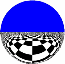
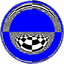
Figure 2: Ray tracing simulations how the ends of wormholes appear when the other ends are above an infinite chess board under a blue sky. On left figure, $\delta<<1$. On right figure, $\delta\approx 1$. Note that the blue is used for clarity; the wormhole construction is monochromatic.

Construction of a wormhole device $N$ in $\mathbb{R}^{3}$ - We next explain how to build a “device” $N$ in $\mathbb{R}^{3}$ which affects the propagation of electromagnetic waves in the same way as the presence of the handle $M_{2}$ in the wormhole manifold $M$. We emphasize that we do not tear and glue “pieces of space”, but instead prescribe a configuration of metamaterials which make the waves behave as if there were an invisible tube attached to the Euclidian space making the distance between points in $M_{1}$ shorter. In the other words, as far as EM observations of the wormhole device are concerned, if appears as if the topology of space has been changed.

We use cylindrical coordinates $(\theta,r,z)$ corresponding to a point $(r\cos\theta,r\sin\theta,z)$ in $\mathbb{R}^{3}$. The wormhole device is built around an obstacle $K\subset\mathbb{R}^{3}$. To define $K$, let $S$ be the two-dimensional finite cylinder $\{\theta\in[0,2\pi],r=2,\ 0\leq z\leq L\}\subset\mathbb{R}^{3}$. The open region $K$ consists of all points in $\mathbb{R}^{3}$ that have distance less than one to $S$ and has the shape of a long, thick-walled tube with smoothed corners.

\psfrag{1}{$A$}\psfrag{2}{$B$}\psfrag{3}{$C$}\psfrag{4}{$D$}\psfrag{5}{$A^{\prime}$}\psfrag{6}{$B^{\prime}$}\psfrag{7}{$C^{\prime}$}\psfrag{8}{$D^{\prime}$}\psfrag{9}{}\includegraphics[width=227.62204pt]{mapf5B.eps}

Let us first introduce a deformation map $F$ from $M$ to $N=\mathbb{R}^{3}\setminus K$ or, more precisely, from $M\setminus\gamma$ to $N\setminus\Sigma$, where $\gamma$ is a closed curve in $M$ to be described shortly and $\Sigma=\partial K$. We will define $F$ separately on $M_{1}$ and $M_{2}$ denoting the corresponding parts by $F_{1}$ and $F_{2}$.

To describe $F_{1}$, let $\gamma_{1}$ be the line segment on the $z-$axis connecting $\partial B({\it O},1)$ and $\partial B(P,1)$ in $M_{1}$, namely, $\gamma_{1}=\{r=0,\ z\in[1,L-1]\}$. Let $F_{1}(r,z)=(\theta,R(r,z),Z(r,z)),$ be such that $(R(r,z),Z(r,z))$, shown in the Figure above, transforms in the $(r,z)$ coordinates the semicircles $AB$ and $CD$ in the left picture to the vertical line segments $A^{\prime}B^{\prime}=\{r\in[0,1],z=0\}$ and $C^{\prime}D^{\prime}=\{r\in[0,1],z=L\}$ in the right picture and the cut $\gamma_{1}$ on the left picture to the curve $B^{\prime}C^{\prime}$ on the right picture. This gives us a map $F_{1}:M_{1}\setminus\gamma_{1}\to N_{1}\setminus\Sigma,$ where the closed region $N_{1}$ in $\mathbb{R}^{3}$ is obtained by rotation of the region exterior to the curve $A^{\prime}B^{\prime}C^{\prime}D^{\prime}$ around the $z-$axis. We can choose $F_{1}$ so that it is the identity map in the domain $U=\mathbb{R}^{3}\setminus\{-2\leq z\leq L+2,\ 0\leq r\leq 4\}$.

To describe $F_{2}$, consider the line segment, $\gamma_{2}=\{NP\}\times[0,1]$ on $M_{2}$ . The sphere without the north pole can be ”flattened” and stretched to an open disc with radius one which, together with stretching $[0,1]$ to $[0,L]$, gives us a map $F_{2}$ from $M_{2}\setminus\gamma_{2}$ to $N_{2}\setminus\Sigma$. The region $N_{2}$ is the $3-$dimensional cylinder, $N_{2}=\{\theta\in[0,2\pi],r\in[0,1],z\in[0,L]\}$. When flattening ${\mathbb{S}}^{2}\setminus NP$, we do it in such a way that $F_{1}$ on $\partial B({\it O},1)$ and $\partial B(P,1)$ coincides with $F_{2}$ on $({\mathbb{S}}^{2}\setminus NP)\times\{0\}$ and $({\mathbb{S}}^{2}\setminus NP)\times\{1\}$, respectively. Thus, $F$ maps $M\setminus\gamma$, where $\gamma=\gamma_{1}\cup\gamma_{2}$ is a closed curve in $M$, onto $N\setminus\Sigma$; in addition, $F$ is the identity on the region $U$.

Next we define the electromagnetic material parameter tensors on $N$. We define the permittivity to be

$$\widetilde{\varepsilon}=F_{*}\varepsilon(y)=\left.\frac{(DF)(x)\cdotp\varepsilon(x)\cdotp(DF(x))^{t}}{\hbox{det}(DF)}\right|_{x=F^{-1}(y)},$$ (3)

where $DF$ is the derivative matrix of $F$, and similarly the permeability to be $\widetilde{\mu}=F_{*}\mu$. These deformation rules are based on the fact that permittivity and permeability are conductivity type tensors, see KLS .

Maxwell’s equations are invariant under smooth changes of coordinates. This means that, by the Chain Rule, any solution to Maxwell’s equations in $M\setminus\gamma$ endowed with material parameters $\varepsilon,\mu$ becomes, after transformation by $F$, a solution to Maxwell’s equations in $N\setminus\Sigma$ with material parameters $\widetilde{\varepsilon}$ and $\widetilde{\mu}$, and vice versa. However, when considering the fields on the entire spaces $M$ and $N$, these observations are not enough, due to the singularities of $\widetilde{\varepsilon}$ and $\widetilde{\mu}$ near $\Sigma$; the significance of this for cloaking has been analyzed in GKLU . In the following, we will show that the physically relevant class of solutions to Maxwell’s equations, namely the (locally) finite energy solutions, remains the same, with respect to the transformation $F$, in $(M;\varepsilon,\mu)$ and $(N;\widetilde{\varepsilon},\widetilde{\mu}).$ One can analyze the rays in $M$ and $N$ endowed with the electromagnetic wave propagation metrics $g=\sqrt{\varepsilon\mu}$ and $\widetilde{g}=\sqrt{\widetilde{\varepsilon}\widetilde{\mu}}$, respectively. Then the rays on $M$ are transformed by $F$ into the rays in $N$. As almost all the rays on $M$ do not intersect with $\gamma$, therefore, almost all the rays on $N$ do not approach $\Sigma$. This was the basis for Le ; PSS1 and was analyzed further in PSS2 ; see also MBW for a similar analysis in the context of elasticity. Thus, heuristically one is led to conclude that the electromagnetic waves on $(M;\varepsilon,\mu)$ do not feel the presence of $\gamma$, while those on $(N;\widetilde{\varepsilon},\widetilde{\mu})$ do not feel the presence of $K$, and these waves can be transformed into each other by the map $F$.

Although the above considerations are mathematically rigorous, on the level both of the Chain Rule and of high frequency limits, i.e., ray tracing, in the exteriors $M\setminus\gamma$ and $N\setminus\Sigma$, they do not suffice to fully describe the behavior of physically meaningful solution fields on $M$ and $N$. However, by carefully examining the class of the finite-energy waves in $M$ and $N$ and analyzing their behavior near $\gamma$ and $\Sigma$, respectively, we can give a complete analysis, justifying the conclusions above. Let us briefly explain the main steps of the analysis using methods developed for theory of invisibility (or cloaking) at frequency $k>0$ GKLU and at frequency $k=0$ in GLU1 ; GLU2 ; full details will be given elsewhere. First, to guarantee that the fields in $N$ are finite energy solutions and do not blow up near $\Sigma$, we have to impose at $\Sigma$ the appropriate boundary condition, namely, the Soft-and-Hard (SH) condition, see HLS ; Ki2 ,

$$e_{\theta}\,\cdotp E|_{\Sigma}=0,\quad e_{\theta}\,\cdotp H|_{\Sigma}=0,$$ (4)

where $e_{\theta}$ is the angular direction. Secondly, the map $F$ can be considered as a smooth coordinate transformation on $M\setminus\gamma$; thus, the finite energy solutions on $M\setminus\gamma$ transform under $F$ into the finite energy solutions on $N\setminus\Sigma$, and vice versa. Thirdly, the curve $\gamma$ on $M$ has Hausdorff dimension equal to one. This implies that the possible singularities of the finite energy electromagnetic fields near $\gamma$ are removable KKM , that is, the finite energy fields in $M\setminus\gamma$ are exactly the restriction to $M\setminus\gamma$ of the fields defined on all of $M$.

Combining these steps we can see that measurements of the electromagnetic fields on $(M;\varepsilon,\mu)$ and on $(\mathbb{R}^{3}\setminus K;\widetilde{\varepsilon},\widetilde{\mu})$ coincide in $U$. In the other words, if we apply any current on $U$ and measure the radiating electromagnetic fields it generates, then the fields on $U$ in the wormhole manifold $(M;\varepsilon,\mu)$ coincide with the fields on $U$ in $(\mathbb{R}^{3}\setminus K;\widetilde{\varepsilon},\widetilde{\mu})$, $3$-dimensional space equipped with the wormhole device construction.

Summarizing our constructions, the wormhole device consists of the metamaterial coating of the obstacle $K$. This coating should have the permittivity $\widetilde{\varepsilon}$ and permeability $\widetilde{\mu}$. In addition, we should impose the SH boundary condition on $\Sigma$, which may be realized by making the obstacle $K$ from a perfectly conducting material with parallel corrugations on its surface HLS ; Ki2 .

The permittivity $\widetilde{\varepsilon}$ and and permeability $\widetilde{\mu}$ may described in a rather simple form. For some potential applications, it is desirable to allow for a solid cylinder around the axis of the wormhole to be consist of a vacuum or air, and it is possible to provide for that using a slightly different construction than was described above, starting with flattened spheres. A physical approximation to the mathematical idealization of the material parameters needed for either of these designs can be implemented using carefully designed concentric rings as in the experimental implementation of cloaking at a microwave frequency SMJCPSS .

Applications - Finally, we consider applications of wormhole devices. The current rapid development of metamaterials designed for microwave and optical frequencies SMJCPSS ; Soukoulis indicates the potential for physical applications of the wormhole construction, which are numerous:

Optical cables. A wormhole device functions as an invisible optical tunnel or cable. In particular, a wormhole device, considered as an invisible tunnel, could be useful in making measurements of electromagnetic fields without disturbing those fields; these tunnels do not radiate energy to the exterior except from their ends.

Virtual magnetic monopoles. Consider a very long invisible tunnel. Assume that one end of the tunnel is located in a region where a magnetic field enters the wormhole. Then the other end of the tunnel behaves like a magnetic monopole, see Frankel .

Optical computers. Wormholes could be used in optical computers. For instance, active components could be located inside wormholes devices having only visible “exits” for input and output.

3D video displays. Divide a cube in $\mathbb{R}^{3}$ to $N\times N\times N$ voxels (three dimensional pixels) and put an end of a invisible tunnel into each voxel. Assume that the end of each tunnel is much smaller than the voxel, so that from the exterior of the cube, all ends of the invisible tunnels are directly visible along any line that does not intersect the other ends of the wormholes. Then, by inserting light from the other ends of these $N^{3}$ invisible tunnels, one could direct light separately to each of the voxels. This creates a device acting as a “three dimensional video display”.

Scopes for MRI devices. We can modify construction of $M_{1}$ and $M_{2}$ by deforming the sphere ${\mathbb{S}}^{2}$ so that it is flat near the south pole $SP$ and the north pole $NP$ and making the tube $M_{2}$ longer; see the supporting online material. This then allows the permittivity $\widetilde{\varepsilon}$ and permeability $\widetilde{\mu}$ in $N$ to be constant near the $z$-axis. This means that inside the wormhole there could be vacuum or air. Thus, for instance, in Magnetic Resonance Imaging (MRI) we could use a wormhole to build a tunnel that would not disturb the homogeneous magnetic field needed for the imaging. Through such a tunnel, or “scope”, magnetic metals and other materials or components can be transported to the imaged area without disturbing the fields. Such tunnels could be useful in medical operations using simultaneous MRI imaging.

Wormholes for beam collimation. Consider a wormhole with a metric that at a point $(y,s)\in{\mathbb{S}}^{2}\times[0,1]$ is the warped product of the standard metric of sphere ${\mathbb{S}}^{2}_{r(s)}$ of radius $r(s)$ and the standard metric of $[0,1]$. Making $r(s)$ very small in the middle of the wormhole produces an approximate cloaking effect GLU1 ; GLU2 , so that only the light rays that travel almost parallel to the axis of the wormhole can pass through it; other rays return back to the same end from which they entered. Thus, a simple configuration of a wormhole and lenses could be used to collimate EM beams.

Acknowledgements: AG and GU are supported by US NSF, ML by Academy of Finland.

References

- (1) U. Leonhardt, Science 312, 1777 (23 June 2006).
- (2) J.B. Pendry, D. Schurig, D.R. Smith, Science 312, 1780 (23 June, 2006).
- (3) J.B. Pendry, D. Schurig, D.R. Smith, Opt. Exp. 14, 9794 (2006).
- (4) U. Leonhardt and T. Philbin, New J. Phys. 8. 247 (2006).
- (5) A. Greenleaf, Y. Kurylev, M. Lassas and G. Uhlmann, to appear in Comm. Math. Phys., Preprint: ArXiv/math.AP/0611185 (2006).
- (6) G. Milton, M. Briane, J. Willis, New J. Phys. 8, 248 (2006).
- (7) M. Lassas, M. Taylor and G. Uhlmann, Commun. Geom. Anal. 11, 207 (2003).
- (8) A. Greenleaf, M. Lassas and G. Uhlmann, Physiol. Meas. 24, 413 (2003).
- (9) A. Greenleaf, M. Lassas and G. Uhlmann, Math. Res. Lett. 10, 685 (2003).
- (10) A. Greenleaf, M. Lassas and G. Uhlmann, Commun. Pure App. Math. 56, 328 (2003).
- (11) D. Schurig et al., Science 314 977 (10 November 2006).
- (12) S. Hawking and G. Ellis, The Large Scale Structure of Space-Time, Camb. U. Pr., 1973.
- (13) M. Visser, Lorentzian Wormholes, AIP Press, 1997.
- (14) Y. Kurylev, M. Lassas, and E. Somersalo, J. Math. Pures et Appl. 86, 237 (2006).
- (15) T. Frankel, The geometry of physics, Camb. U. Pr., 1997.
- (16) A. Bossavit Électromagnètisme, en vue de la modèlisation. (Springer-Verlag, 1993).
- (17) T. Kilpeläinen, J. Kinnunen and O. Martio, Potential Anal. 12, 233 (2000).
- (18) I. Hänninen, I. Lindell and A. Sihvola, Prog. in Electromag. Res. 64, 317(2006).
- (19) P. S. Kildal, IEEE Trans. on Ant. and Propag. 10, 1537 (1990).
- (20) C. Soukoulis, S. Linden, and M. Wegener, Science 315, 47 ( 5 January 2007).