\catchline

Approximations of singular vertex couplings in quantum graphs

PAVEL EXNER Doppler Institute for Mathematical Physics and Applied Mathematics, Czech Technical University, Břehová 7, 11519 Prague, Czech Republic
exner@ujf.cas.cz
   ONDŘEJ TUREK Department of Mathematics, Faculty of Nuclear Sciences and Physical Engineering, Czech Technical University, Trojanova 13, 12000 Prague, Czech Republic
oturek@centrum.cz
((Day Month Year); (Day Month Year))
Abstract

We discuss approximations of the vertex coupling on a star-shaped quantum graph of $n$ edges in the singular case when the wave functions are not continuous at the vertex and no edge-permutation symmetry is present. It is shown that the Cheon-Shigehara technique using $\delta$ interactions with nonlinearly scaled couplings yields a $2n$-parameter family of boundary conditions in the sense of norm resolvent topology. Moreover, using graphs with additional edges one can approximate the ${n+1\choose 2}$-parameter family of all time-reversal invariant couplings.

keywords:
quantum graph, vertex conditions, approximations, point interactions
{history}
\ccode

Mathematics Subject Classification 2000: 81Q10

1 Introduction

The concept of quantum mechanics on a graph is more than half a century old having roots in modelling of aromatic hydrocarbons [1]. For many years, however, it was rather a curiosity, or maybe an interesting textbook example. The situation changed two decades ago with the advent of microfabrication techniques which allow us to produce tiny graph-shaped structures of semiconductor and other materials for which this is a useful and versatile model. This motivated a new theoretical attention to the subject – see, e.g., [2, 3]. Since then the literature on quantum graphs grew to a formidable volume, and we restrict ourselves here to mentioning recent reviews in [4, 5, 6] where an extensive bibliography can be found.

From the mathematical point of view the attractive feature of the model is that it deals with families of ordinary differential equations, the solutions of which have to be properly matched at the graph edge endpoints. Since the solutions are often explicitly known, the spectral analysis can be reduced to an algebraic problem.

The key point here are the boundary conditions through which the wave functions are matched. The Hamiltonian is typically a second-order differential operator, for instance, in the simplest case of a free spinless particle it acts on the $j$-th edge as $H\psi_{j}=-\psi^{\prime\prime}_{j}$. Thus the boundary conditions are linear relations coupling the values of the functions and their first derivatives at graph vertices; from the physical point of view it is usually sufficient to consider only local couplings which involve values at a single vertex only. Another general physical restriction is the self-adjointness of the Hamiltonian; it implies that a vertex joining $n$ graph edges may be characterized by boundary conditions involving $n^{2}$ real parameters [3].

This leaves a considerable freedom in the choice of a model to describe particular physical systems, and an understanding of the physical meaning of vertex coupling is needed to pick the appropriate operator from the class of admissible Hamiltonians. A natural way to approach this problem is through approximation, i.e. regarding the quantum graph in question as a limit of a family of more “realistic” systems with a less number of free parameters. One possibility is to approximate a graph by a family of “fat graphs” or similar manifolds equipped with the corresponding Laplace-Beltrami operators. The best studied case is the one where the approximated manifolds have Neumann boundary, or no boundary et all [7, 8, 9, 10, 11, 12], where unfortunately the limit yields – of the multitude of available boundary conditions – only the most simple ones. There are also fresh results [13, 14] on the case with Dirichlet boundary but in general the approach based on squeezed manifolds did not yield so far a satisfactory answer to the question.

Another, maybe less ambitious approach is to model vertex boundary conditions through families of interactions on the graph itself. Here two cases have to be distinguished. In the $n^{2}$-parameter family mentioned above the boundary conditions with wave functions continuous at the vertex form just one-parameter subfamily. These boundary conditions can be approximated by families of scaled potentials in analogy is analogy with one-dimensional $\delta$ interactions [15]. The remaining, more singular cases require a different approach. An inspiration may be derived from the approximation of one-dimensional $\delta^{\prime}$ interactions suggested, somewhat surprisingly, by Cheon and Shigehara in [16] and elaborated in a mathematically consistent way in [17, 18]. It is based on a family of $\delta$ interactions which approach each other being scaled in a particular nonlinear way. An analogous procedure for vertices of degree $n\geq 2$ was proposed in [19] in the case of the so-called $\delta^{\prime}_{s}$ coupling; the key element here was the symmetry with respect to permutation of the edges which allowed to reduce the analysis to a one-dimensional halfline problem. The same technique was afterwards in [20] applied to the class of all permutation-symmetric boundary conditions which form a two-parameter subfamily in the $n^{2}$-parameter set.

The main goal of the present paper is to explore whether the idea of [16] can be adapted to situations without a permutation symmetry and how wide class of boundary conditions can be in this way described. As in the work mentioned above we will consider a star graph with a single vertex and $n$ semi-infinite edges. For simplicity we will also assume that the motion on graphs edges is free; the obtained approximations extend easily to Schrödinger operators on the graph provided the potentials involved are sufficiently regular around the vertex. We are going to show that the Cheon-Shigehara technique can produce for $n>2$ at most a $2n$-parameter family of boundary conditions at the vertex. Furthermore, we will demonstrate that such an approximations, with two $\delta$ interaction at each edge, do indeed exist and that they converge in the norm resolvent topology.

The next question is how to extend the approximation to a wider class of couplings. A natural possibility is amend the star by extra edges supporting $\delta$ interactions which shrink to the “main” vertex with the parameter controlling the approximation. We devise such a scheme a show that it yields an ${n+1\choose 2}$-parameter family, generically all couplings which are time-reversal invariant. In this case, however, we restrict ourselves to deriving the boundary condition formally. We are convinced that the norm resolvent convergence could be verified as in the case mentioned but the argument would be extremely cumbersome. Notice that the idea of using additional edges to model singular couplings appeared already in [21]. In contrast to that paper, however, we keep here the number of added edges fixed.

Let us review briefly the contents of the paper. In the next section we gather the needed preliminary information. We review the quantum graph concept, recall different vertex couplings and review briefly the known approximations. In Section 3 we analyze a CS-type approximation to the vertex in a star graph based on adding $\delta$ interactions on star edges, the following section is devoted to the proof of norm-resolvent convergence. Finally, in Section 5 we will describe the mentioned more general approximation with extra edges added to the star graph.

2 Preliminaries

2.1 Quantum graphs

Let us first recall a few basic notions. A graph $\Gamma$ is an ordered pair $\Gamma=(V,E)$, where $V$ and $E$ are finite or countably infinite sets of vertices and edges, respectively. Without loss of generality we may identify $E$ with a family of two-element subsets in $V$, excluding thus loops and multiple edges, since in the opposite case we can simply add extra vertices. The vertex degree of $v\in V$ is the number of edges which have $v$ as its endpoint. $\Gamma$ is a metric graph if each of its edges can be equipped with a distance, i.e. identified with a finite or semi-infinite interval of length $\ell\in(0,+\infty]$; the endpoints “at infinity” are conventionally not counted as vertices. In particular a star graph has a finite number $n\geq 2$ of edges and a single centre which is the only vertex where all the edges (called also arms in this case) meet.

The subject of our interest is quantum mechanics on graphs. Given a metric graph $\Gamma$ with edges $J_{1},\dots,J_{n}$ we identify the orthogonal sum $\mathcal{H}=\bigoplus_{j=1}^{n}L^{2}(J_{j})$ with the state Hilbert space, i.e. the wave function of a spinless particle “living” on $\Gamma$ can be written as the column $\Psi=(\psi_{1},\psi_{2},\ldots,\psi_{n})^{T}$ with $\psi_{j}\in L^{2}(J_{j})$. In the absence of external fields the Hamiltonian $H$ acts as $(H_{\Gamma}\Psi)_{j}=-\psi^{\prime\prime}_{j}$, where as usual we put $\hbar=2m=1$. Its domain consists of functions from $W^{2,2}(\Gamma):=\bigoplus_{j=1}^{n}W^{2,2}(J_{j})$; since $H$ is required to be a self-adjoint operator they must satisfy appropriate boundary conditions at the vertices which we will recall below.

The meaning of these boundary condition is our main concern in this paper, therefore we restrict ourselves to graphs with a single vertex, namely star graphs with $n$ semi-infinite edges $J_{j}\simeq\mathbb{R}^{+},\>j=1,\dots,n$; we denote them as $\Gamma$ or $\Gamma_{n}$.

2.2 Vertex couplings

Since the Hamiltonian mentioned above is a second-order operator, the matching conditions involve boundary values of the functions in the vertex and of their first derivatives. Both regarded as one-sided limits, the derivatives are taken in the outward direction. We arrange them into column vectors $\Psi(0)$ and $\Psi^{\prime}(0)$. The self-adjointness of $H$, which in the physical language means conservation of probability current at the vertex, is expressed through a linear relation between these vectors,

$$A\Psi(0)+B\Psi^{\prime}(0)=0\,,$$ (1)

by [22] the operator $H$ is self-adjoint if and only if $A,B\in\mathbb{C}^{n,n}$ satisfy the conditions

$$\mathrm{rank}(A,B)=n\,,\quad AB^{*}\textrm{\;\;is self-adjoint},$$ (2)

where $(A,B)$ denotes the $n\times 2n$ matrix with $A,B$ forming the first and the second $n$ columns, respectively. This parametrization is obviously non-unique, since $A,B$ can be replaced by $CA,CB$ with any regular $n\times n$ matrix $C$. This defect can be corrected by choosing the matrices in the standard form [23, 24],

$$(U-I)\Psi(0)+\mathrm{i}(U+I)\Psi^{\prime}(0)=0\,,$$ (3)

where $U$ is an $n\times n$ unitary matrix; the Hamiltonian corresponding to this condition will be labelled as $H_{U}$. Elements of this family are labelled by $n^{2}$ real parameters which is, of course, the right number because all the $H_{U}$ are self-adjoint extensions of a common symmetric restriction with deficiency indices $(n,n)\,$ [3].

Let us next recall a few examples of the boundary conditions (3). As mentioned in the introduction, the requirement of continuity at the vertex selects a one-parameter subfamily corresponding to the so-called $\delta$ coupling,

$$\psi_{j}(0)=\psi_{k}(0)=:\psi(0)\,,\quad j,k\in\hat{n}\,,\qquad\sum^{n}_{j=1}\psi_{j}^{\prime}(0)=\alpha\psi(0)\,,$$ (4)

where $\alpha\in\mathbb{R}$ and for brevity we have introduced the symbol $\hat{n}:=\{1,2,\ldots,n\}$. We can add the case corresponding formally to $\alpha=\infty$, when the system decomposes into $n$ halflines with Dirichlet endpoints, however, it is not interesting as long as we are concerned with nontrivial vertex couplings. In the particular case $\alpha=0$ we speak about free boundary conditions since for the $\delta$ function on line, $n=2$, this corresponds to a free motion (sometimes the term Kirchhoff b.c., not very appropriate, is used). In terms of (3) the $\delta$ coupling corresponds to the matrix $U=\frac{2}{n+\mathrm{i}\alpha}\mathcal{J}-I$, where $\mathcal{J}$ denotes the $n\times n$ matrix whose all entries equal one.

The $\delta^{\prime}$ interaction on the line has two possible analogues for $n>2\,$ [25, 26]. One is a counterpart to (4) called $\delta^{\prime}_{s}$ coupling with the role of $\Psi(0),\,\Psi^{\prime}(0)$ interchanged,

$$\psi_{j}^{\prime}(0)=\psi_{k}^{\prime}(0)=:\psi^{\prime}(0)\,,\quad j,k\in\hat{n}\,,\qquad\sum^{n}_{j=1}\psi_{j}(0)=\beta\psi^{\prime}(0)\,,$$ (5)

where $\beta\in\mathbb{R}\cup\{+\infty\}$. It corresponds to $U=I-\frac{2}{n-\mathrm{i}\beta}\mathcal{J}$, in particular, the case $\beta=\infty$ refers to full Neumann decoupling. The other one, called $\delta^{\prime}$ coupling, is

$$\sum^{n}_{j=1}\psi_{j}^{\prime}(0)=0\,,\qquad\psi_{j}(0)-\psi_{k}(0)=\frac{\beta}{n}\left(\psi_{j}^{\prime}(0)-\psi_{k}^{\prime}(0)\right)\quad j,k\in\hat{n}\,,$$ (6)

with $\beta\in\mathbb{R}\cup\{+\infty\}$ which corresponds to $U=-\frac{n+\mathrm{i}\beta}{n-\mathrm{i}\beta}I+\frac{2}{n-\mathrm{i}\beta}\mathcal{J}$.

All the above examples have a common property, namely that the corresponding operators are invariant with respect to permutation of the edges, which is clear from the fact that matrices $U$ are not changed by a simultaneous permutations of the rows and columns. The most general family of $H_{U}$ with this property is characterized by two parameters, $U=aI+bJ$ with $|a|=1$ and $|a+nb|=1$, cf. [20], the corresponding boundary conditions being

$\displaystyle(a-1)\left(\psi_{j}(0)-\psi_{k}(0)\right)+\mathrm{i}(a+1)\left(\psi_{j}^{\prime}(0)-\psi_{k}^{\prime}(0)\right)$ $\displaystyle=$ $\displaystyle 0\,,\quad j,k\in\hat{n}\,,$
$\displaystyle(a-1+nb)\sum^{n}_{k=1}\psi_{k}(0)+\mathrm{i}(a+1+nb)\sum^{n}_{k=1}\psi_{k}^{\prime}(0)$ $\displaystyle=$ $\displaystyle 0\,.$

2.3 Approximation of $\delta$ couplings

Let us next recall briefly known results about approximations of vertex couplings starting from the $\delta$ coupling. The idea is the same as for $\delta$ interactions on the line.

Let $U_{\delta}(\alpha):=\frac{2}{n+\mathrm{i}\alpha}\mathcal{J}-I$ be the corresponding matrix of the condition (3). Given a family of real-valued functions $W=\{W_{j}:\>j\in\hat{n}\}$, for simplicity assumed to be compactly supported, we define scaled potentials at graph edges by

$$W_{\epsilon,j}\,:=\,\frac{1}{\epsilon}\,W_{j}\left(x\over\epsilon\right)\,,\quad j\in\hat{n}\,.$$ (8)

Starting from the free boundary conditions and choosing the family (8) we can approximate any nontrivial $\delta$ coupling as the following result shows.

Theorem 2.1.

Suppose that $W_{j}\in L^{1}(0,1)$ for $j\in\hat{n}$, then

$$H_{U_{\delta}(0)}+W_{\epsilon}\,\longrightarrow\,H_{U_{\delta}(\alpha)}\;\quad\mathrm{as}\quad\epsilon\to 0+$$ (9)

in the norm resolvent sense, where $\,\alpha:=\sum_{j=1}^{n}\int_{0}^{1}W_{j}(x)\,dx\,$.

For proof see [15] where a more general result of this type is derived, together with other extensions of the standard Sturm-Liouville theory to star graphs.

2.4 Approximation of singular permutation-invariant couplings

Consider further permutation-invariant couplings with wave functions discontinuous at the vertex. Denote the operator $H_{U}$ corresponding to $U=aI+bJ$ with $a,b$ satisfying the stated conditions as $H^{a,b}$. The approximating family can be constructed as follows: we start from the operator $H_{u,0}:=H_{U_{\delta}(u)}$ and pass to $H_{u,v}$ obtained by adding a $\delta$ interaction of strength $v$ on each edge at a distance $d$ from the centre. We will let the $\delta$’s approach the centre scaling properly $u,v$.

Theorem 2.2.

Fix a pair of complex numbers $a\neq-1$ and $b\neq 0$ such that $|a|=1$ and $|a+nb|=1$, and set

$$u(d):=\mathrm{i}\frac{n}{d^{2}}\left(\frac{a-1+nb}{a+1+nb}+\frac{a-1}{a+1}\right)^{-1}\,,\quad v(d):=-\frac{1}{d}-\mathrm{i}\frac{a-1}{a+1}\,.$$ (10)

Suppose that $a+1+nb\neq 0$ and $a(a+nb)\neq 1$, then the operators $H_{u(d),v(d)}$ converge to $H^{a,b}$ in the norm resolvent topology as $d\to 0+$. Moreover, the claim remains true in the two excluded cases, provided we replace the above $u(d)$ by $-nd^{-1}$ and $\zeta d^{-\nu}$ with $\mathbb{R}\ni\zeta\neq 0$ and $\nu>2$, respectively.

Proof can be found in [20], the particular case of $\delta^{\prime}_{s}$ coupling (5) in which $u(d)=-\beta d^{-2}$ and $v(d)=-d^{-1}$ was discussed in [19].

3 CS-type approximation of singular couplings

After the preliminaries let us turn to our proper task, namely approximations of singular couplings à la Cheon and Shigehara, i.e. by means of additional $\delta$ interactions, properly scaled, on edges of our star graph, without the requirement of permutation invariance.

3.1 The class of approximable couplings

The first question is how large is the class of operators $H_{U}$ which can can be treated in this way. We are going to answer it using the technique of [16], i.e. looking into convergence of the corresponding boundary conditions.

Proposition 3.1.

Let $\Gamma$ be a star graph with $n$ semi-infinite edges and $\Gamma(d)$ be a graph obtained from $\Gamma$ by adding a finite number of vertices at each edge. Consider a family $\left\{\Gamma(d):\>d\in\mathbb{R}^{+}\right\}$ of such graphs with the properties that the number of the added vertices at each edge is independent of $d$ and their distances from the centre are $\mathcal{O}(d)$ as $d\to 0_{+}$. Suppose that a family of functions $\Psi_{d}\in W^{2,2}\left(\Gamma\setminus(\{c\}\cup V_{d})\right)$, where $c$ is the centre of $\Gamma$ and $V_{d}$ is the set of added vertices, satisfies the conditions (4) with $d$-dependent parameters, and that it converges to $\Psi\in W^{2,2}\left(\Gamma\setminus\{c\}\right)$ which obeys the condition (1) with some $A,\,B$ satisfying the requirements (2). The family of the conditions (1) which can be obtained in this way depends on $2n$ parameters if $n>2$, and on three parameters for $n=2$.

Proof 3.2.

The $\delta$ coupling in the centre of $\Gamma$ is expressed by the condition (4). Consider first $\delta$ interactions on a halfline and look how the boundary values change when we pass between different sites. Suppose that at a point $x$ the function and its derivative have the right limits, and that $x+\epsilon$ is the site of a $\delta$ interaction, then the Taylor expansion gives

$$\psi(x+\epsilon_{-})=\psi(x_{+})+\epsilon\psi^{\prime}(x_{+})+\mathcal{O}(\epsilon^{2})\,,\quad\psi^{\prime}(x+\epsilon_{-})=\psi^{\prime}(x_{+})+\mathcal{O}(\epsilon)\,,$$

and the $\delta$ interaction is according to (4) described by

$$\psi(x+\epsilon_{+})=\psi(x+\epsilon_{-})=:\psi(x+\epsilon)\,,\qquad\psi^{\prime}(x+\epsilon_{+})-\psi^{\prime}(x+\epsilon_{-})=\alpha(\epsilon)\psi(x+\epsilon)\,,$$

where $\alpha(\epsilon)$ is the coupling parameter. The may be $\epsilon$-dependent but we suppose such a dependence that the error terms can be neglected as $\epsilon\to 0_{+}$; then we have

$\displaystyle\psi(x+\epsilon)$ $\displaystyle=\psi(x_{+})+\epsilon\psi^{\prime}(x_{+})+\mathcal{O}(\epsilon^{2})\,,$
$\displaystyle\psi^{\prime}(x+\epsilon_{+})$ $\displaystyle=\psi^{\prime}(x_{+})+\mathcal{O}(\epsilon)+\alpha(\epsilon)(\psi(x_{+})+\epsilon\psi^{\prime}(x_{+})+\mathcal{O}(\epsilon^{2}))=$
$\displaystyle=(1+\alpha(\epsilon)\epsilon)\psi^{\prime}(x_{+})+\alpha(\epsilon)\psi(x_{+})+\mathcal{O}(\epsilon)+\alpha(\epsilon)\mathcal{O}(\epsilon^{2})\,,$

so that $\psi(x+\epsilon)$ and $\psi^{\prime}(x+\epsilon_{+})$ depend on $\psi(x_{+})$ and $\psi^{\prime}(x_{+})$ linearly up to error terms. In case of a finite number of $\delta$ interactions on a halfline one can show in a similar way recursively that the function value and the right limit of the derivative at the site of the last $\delta$ depends, up to error terms, linearly on the function value and the right limit of the derivative for the first $\delta$ interaction.

Let us apply this conclusion to the edges of our star graph. We denote by $d_{j}$ the distance of the last $\delta$ interaction on the $j$-th halfline family of edges in $\Gamma(d)$; by assumption we have $d_{j}=\mathcal{O}(d)$. Then we have

$\displaystyle\tilde{f}^{(1)}_{j}(d)\psi_{j}(d_{j})$ $\displaystyle=$ $\displaystyle\tilde{g}^{(1)}_{j}(d)\psi(0)+\tilde{h}^{(1)}_{j}(d)\psi_{j}^{\prime}(0)+\tilde{r}^{(1)}_{j}(d)\,,$
$\displaystyle\tilde{f}^{(2)}_{j}(d)\psi_{j}^{\prime}({d_{j}}_{+})$ $\displaystyle=$ $\displaystyle\tilde{g}^{(2)}_{j}(d)\psi(0)+\tilde{h}^{(2)}_{j}(d)\psi_{j}^{\prime}(0)+\tilde{r}^{(2)}_{j}(d)$

for some $\tilde{f}^{(1)}_{j},\tilde{g}^{(1)}_{j},\tilde{h}^{(1)}_{j},\tilde{f}^{(2)}_{j},\tilde{g}^{(2)}_{j},\tilde{h}^{(2)}_{j}:\mathbb{R}^{+}\to\mathbb{R}$. The functions $\tilde{r}^{(1)}_{j}$ and $\tilde{r}^{(2)}_{j}(d)$ are error terms and we suppose that they can be neglected in the limit. We are interested in the situation when the last relations can be inverted and $\psi(0),\,\psi_{j}^{\prime}(0)$ can be expressed by means of $\psi_{j}(d_{j})$ and $\psi_{j}^{\prime}({d_{j}}_{+})$,

$\displaystyle\psi(0)$ $\displaystyle=$ $\displaystyle f^{(1)}_{j}(d)\psi_{j}(d_{j})+g^{(1)}_{j}(d)\psi_{j}^{\prime}({d_{j}}_{+})+\mathcal{R}(d)\,,\quad j\in\hat{n}\,,$ (11)
$\displaystyle\psi_{j}^{\prime}(0)$ $\displaystyle=$ $\displaystyle\tilde{f}^{(2)}_{j}(d)\psi_{j}(d_{j})+\tilde{g}^{(2)}_{j}(d)\psi_{j}^{\prime}({d_{j}}_{+})+\mathcal{R}(d)\,,\quad\;\,j\in\hat{n}\,,$ (12)

where we have introduced $\mathcal{R}(d)$ as the symbol for a generic remainder; we still assume that it can be neglected with respect to the other terms as $d\to 0_{+}$. The equations (11) yield for $j,k\in\hat{n}$ the conditions

$$f^{(1)}_{j}(d)\psi_{j}(d_{j})-f^{(1)}_{k}(d)\psi_{k}(d_{k})+g^{(1)}_{j}(d)\psi_{j}^{\prime}({d_{j}}_{+})-g^{(1)}_{k}(d)\psi_{k}^{\prime}({d_{k}}_{+})=\mathcal{R}(d)\,,\quad j,k\in\hat{n}$$ (13)

and from (12) together with the second one of the conditions (4) we get

$$\alpha\psi(0)=\sum^{n}_{k=1}\left(f^{(2)}_{k}(d)\psi_{k}(d_{k})+g^{(2)}_{k}(d)\psi_{k}^{\prime}({d_{k}}_{+})\right)+\mathcal{R}(d)\,.$$ (14)

We substitute for $\psi(0)$ from (11) and perform a repeated summation of (14) over $j$. After an easy rearrangement we get

$$\sum^{n}_{j=1}\left(\alpha f^{(1)}_{j}(d)-nf^{(2)}_{j}(d)\right)\psi_{j}(d_{j})+\sum^{n}_{j=1}\left(\alpha g^{(1)}_{j}(d)-ng^{(2)}_{k}(d)\right)\psi_{j}^{\prime}({d_{j}}_{+})=\mathcal{R}(d)\,.$$ (15)

Now we pass to the limit $d\to 0_{+}$ in the equations (13) and (15). Before that we multiply both sides by a power of $d$ such that the right-hand side tends to zero as $d\to 0_{+}$, while at least one coefficient at the left-hand side remains nonzero, in other words, we use the assumed existence of the limit in which the error terms can be neglected w.r.t. the leading ones. The equation (13) acquires then the form

$$c_{j}\psi_{j}(0)-c_{k}\psi_{k}(0)+t_{j}\psi_{j}^{\prime}(0_{+})-t_{k}\psi_{k}^{\prime}(0_{+})=0\,,\quad j,k\in\hat{n}$$ (16)

while (15) gives

$$\sum^{n}_{j=1}\gamma_{j}\psi_{j}(0)+\sum^{n}_{j=1}\tau_{j}\psi_{j}^{\prime}(0_{+})=0\,,$$ (17)

where $c_{j},\,t_{j},\,\gamma_{j},\,\tau_{j}$ are the appropriate limiting values of the functions involved. The obtained conditions can also be written in a matrix form,

$$\underbrace{\left(\begin{array}[]{ccccc}c_{1}&-c_{2}&0&\cdots&0\\ c_{1}&0&-c_{3}&\cdots&0\\ \vdots&&&\ddots&\\ c_{1}&0&0&\cdots&-c_{n}\\ \gamma_{1}&\gamma_{2}&\gamma_{3}&\cdots&\gamma_{n}\end{array}\right)}_{A}\Psi(0)+\underbrace{\left(\begin{array}[]{ccccc}t_{1}&-t_{2}&0&\cdots&0\\ t_{1}&0&-t_{3}&\cdots&0\\ \vdots&&&\ddots&\\ t_{1}&0&0&\cdots&-t_{n}\\ \tau_{1}&\tau_{2}&\tau_{3}&\cdots&\tau_{n}\end{array}\right)}_{B}\Psi^{\prime}(0)=0\,.$$ (18)

It is clear already now – from the fact that the coefficients $c_{j},\,t_{j},\,\gamma_{j},\,\tau_{j},\>j\in\hat{n}$ are real-valued – that the achievable number of parameters cannot exceed $4n$.

So far we have not brought the self-adjointness into the game. To find the true number of parameters we pass from $A,\,B$ to the unitary matrix $U$ of standard boundary conditions (3). This is achieved by multiplying the relation (18) from the left by a regular matrix $M$ such that $U-I=MA$ and $\mathrm{i}(U+I)=MB$. This determines $U$ since the last relations imply

$$U=\frac{1}{2}M(A-\mathrm{i}B)\,,\quad I=-\frac{1}{2}M(A+\mathrm{i}B)\,;$$

notice that $A+\mathrm{i}B$ is regular because $A$ and $B$ are real and the matrix $(A|B)$ has he full rank by assumption. Hence we have $M=-2(A+\mathrm{i}B)^{-1}$, which further gives

$$U=-(A+\mathrm{i}B)^{-1}\cdot(A-\mathrm{i}B)\,.$$

We shall apply the Gauss elimination method to get the chain of equivalences

$$\bigl{(}-(A+\mathrm{i}B)|(A-\mathrm{i}B)\bigr{)}\sim\cdots\sim\bigl{(}I|\underbrace{-(A+\mathrm{i}B)^{-1}\cdot(A-\mathrm{i}B)}_{U}\bigr{)}\,;$$

the explicit form of $A\pm iB$ is obtained from (18). We notice that the regularity of $A+iB$ implies the following facts: (i) there is at most one $j\in\hat{n}$ such that $c_{j}+\mathrm{i}t_{j}=0$ (and for such a $j$ it holds that $\gamma_{j}+\mathrm{i}\tau_{j}\neq 0$), (ii) there is at least one $j\in\hat{n}$ such that $\gamma_{j}+\mathrm{i}\tau_{j}\neq 0$. The matrix $\bigl{(}-(A+\mathrm{i}B)|(A-\mathrm{i}B)\bigr{)}$ equals to

$$\left(\begin{array}[]{cccc}-(c_{1}+\mathrm{i}t_{1})&c_{2}+\mathrm{i}t_{2}&\cdots&0\\ -(c_{1}+\mathrm{i}t_{1})&0&\cdots&0\\ \vdots&&\ddots&\\ -(c_{1}+\mathrm{i}t_{1})&0&\cdots&c_{n}+\mathrm{i}t_{n}\\ -(\gamma_{1}+\mathrm{i}\tau_{1})&-(\gamma_{2}+\mathrm{i}\tau_{2})&\cdots&-(\gamma_{n}+\mathrm{i}\tau_{n})\end{array}\vline\begin{array}[]{cccc}c_{1}-\mathrm{i}t_{1}&-(c_{2}-\mathrm{i}t_{2})&\cdots&0\\ c_{1}-\mathrm{i}t_{1}&0&\cdots&0\\ \vdots&&\ddots&\\ c_{1}-\mathrm{i}t_{1}&0&\cdots&-(c_{n}-\mathrm{i}t_{n})\\ \gamma_{1}-\mathrm{i}\tau_{1}&\gamma_{2}-\mathrm{i}\tau_{2}&\cdots&\gamma_{n}-\mathrm{i}\tau_{n}\end{array}\right)\,.$$

Suppose first that $c_{j}+\mathrm{i}t_{j}\neq 0$ for all $j\in\hat{n}$, then by equivalent row manipulations we pass to the matrix $(D|V)$, where

$\displaystyle D$ $\displaystyle=\left(\begin{array}[]{ccccc}-\left(\gamma_{1}+\mathrm{i}\tau_{1}+(c_{1}+\it_{1})\sum^{n}_{\ell=1}\frac{\gamma_{\ell}+\mathrm{i}\tau_{\ell}}{c_{\ell}+\mathrm{i}t_{\ell}}\right)&0&0&\cdots&0\\ 0&c_{2}+\mathrm{i}t_{2}&0&\cdots&0\\ 0&0&c_{3}+\mathrm{i}t_{3}&\cdots&0\\ \vdots&&&\ddots&\\ 0&0&0&\cdots&c_{n}+\mathrm{i}t_{n}\end{array}\right),$
$\displaystyle V$ $\displaystyle=\left(\begin{array}[]{cccc}(c_{1}-\mathrm{i}t_{1})S-2\mathrm{i}\frac{c_{1}\tau_{1}-\gamma_{1}t_{1}}{c_{1}+\mathrm{i}t_{1}}&-2\mathrm{i}\frac{c_{2}\tau_{2}-\gamma_{2}t_{2}}{c_{2}+\mathrm{i}t_{2}}&\cdots&-2\mathrm{i}\frac{c_{n}\tau_{n}-\gamma_{n}t_{n}}{c_{n}+\mathrm{i}t_{n}}\\ \frac{2\mathrm{i}}{S}\frac{c_{1}\tau_{1}-\gamma_{1}t_{1}}{c_{1}+\mathrm{i}t_{1}}&-c_{2}+\mathrm{i}t_{2}+\frac{2\mathrm{i}}{S}\frac{c_{2}\tau_{2}-\gamma_{2}t_{2}}{c_{2}+\mathrm{i}t_{2}}&\cdots&\frac{2\mathrm{i}}{S}\frac{c_{n}\tau_{n}-\gamma_{n}t_{n}}{c_{n}+\mathrm{i}t_{n}}\\ \vdots&&\ddots&\\ \frac{2\mathrm{i}}{S}\frac{c_{1}\tau_{1}-\gamma_{1}t_{1}}{c_{1}+\mathrm{i}t_{1}}&\frac{2\mathrm{i}}{S}\frac{c_{2}\tau_{2}-\gamma_{2}t_{2}}{c_{2}+\mathrm{i}t_{2}}&\cdots&-c_{n}+\mathrm{i}t_{n}+\frac{2\mathrm{i}}{S}\frac{c_{n}\tau_{n}-\gamma_{n}t_{n}}{c_{n}+\mathrm{i}t_{n}}\\ \end{array}\right),$

where we have denoted $S=\sum^{n}_{\ell=1}\frac{\gamma_{\ell}+\mathrm{i}\tau_{\ell}}{c_{\ell}+\mathrm{i}t_{\ell}}$. Since we used only equivalent manipulations, the diagonal matrix $D$ should have the same rank as $A+\mathrm{i}B$, hence it must be regular because none of its diagonal elements is zero. Consequently, we can divide each row of $(D|V)$ by the corresponding diagobal element of $D$. This yields $(I|U)$, where $U$ is the sought unitary matrix and its diagonal and off-diagonal elements are given by

$\displaystyle U_{jj}$ $\displaystyle=\frac{2\mathrm{i}(c_{j}\tau_{j}-t_{j}\gamma_{j})}{(c_{j}+\mathrm{i}t_{j})^{2}\sum^{n}_{\ell=1}\frac{\gamma_{\ell}+\mathrm{i}\tau_{\ell}}{c_{\ell}+\mathrm{i}t_{\ell}}}-\frac{c_{j}-\mathrm{i}t_{j}}{c_{j}+\mathrm{i}t_{j}}\,,$ (19)
$\displaystyle U_{jk}$ $\displaystyle=\frac{2i(c_{k}\tau_{k}-t_{k}\gamma_{k})}{(c_{j}+\mathrm{i}t_{j})(c_{k}+\mathrm{i}t_{k})\sum^{n}_{\ell=1}\frac{\gamma_{\ell}+\mathrm{i}\tau_{\ell}}{c_{\ell}+\mathrm{i}t_{\ell}}}\quad\;\mathrm{if}\quad j\neq k\,.$

The right-hand sides make sense due to the first of the conditions (2) and our assumptions about non-vanishing of all the expressions $c_{j}+it_{j}$.

So far we have not employed the second one of the requirements (2), namely the self-adjointness of the matrix $AB^{*}$. This is equivalent to unitarity of $U$, however, it is easier to check it in its original version. By a straightforward computation we find that the product $AB^{*}=AB^{T}$ equals

$$\left(\begin{array}[]{ccccccc}c_{1}t_{1}+c_{2}t_{2}&c_{1}t_{1}&c_{1}t_{1}&\cdots&&c_{1}t_{1}&c_{1}\tau_{1}-c_{2}\tau_{2}\\ c_{1}t_{1}&c_{1}t_{1}+c_{3}t_{3}&c_{1}t_{1}&\cdots&&c_{1}t_{1}&c_{1}\tau_{1}-c_{3}\tau_{3}\\ c_{1}t_{1}&c_{1}t_{1}&c_{1}t_{1}+c_{4}t_{4}&\cdots&&c_{1}t_{1}&c_{1}\tau_{1}-c_{4}\tau_{4}\\ \vdots&&&\ddots&&\vdots\\ c_{1}t_{1}&c_{1}t_{1}&c_{1}t_{1}&\cdots&&c_{1}t_{1}+c_{n}t_{n}&c_{1}\tau_{1}-c_{n}\tau_{n}\\ \gamma_{1}t_{1}-\gamma_{2}t_{2}&\gamma_{1}t_{1}-\gamma_{3}t_{3}&\gamma_{1}t_{1}-\gamma_{4}t_{4}&\cdots&&\gamma_{1}t_{1}-\gamma_{n}t_{n}&\gamma_{1}\tau_{1}+\gamma_{2}\tau_{2}+\cdots\gamma_{n}\tau_{n}\end{array}\right)\,,$$

hence $AB^{*}$ is self-adjoint if and only if $c_{1}\tau_{1}-c_{j}\tau_{j}=\gamma_{1}t_{1}-\gamma_{j}t_{j}$ holds for all $j=2,\ldots,n$, and therefore

$$c_{1}\tau_{1}-\gamma_{1}t_{1}=c_{2}\tau_{2}-\gamma_{2}t_{2}=c_{3}\tau_{3}-\gamma_{3}t_{3}=\cdots=c_{n}\tau_{n}-\gamma_{n}t_{n}\,.$$ (20)

We denote the common value $c_{j}\tau_{j}-\gamma_{j}t_{j}$ as $\kappa$ and recall that we have denoted $S=\sum^{n}_{\ell=1}\frac{\gamma_{\ell}+\mathrm{i}\tau_{\ell}}{c_{\ell}+\mathrm{i}t_{\ell}}$, then the matrix $U$ given by (19) can be simplified,

$$U=\left(\begin{array}[]{cccc}\frac{2\mathrm{i}\kappa}{(c_{1}+\mathrm{i}t_{1})^{2}S}-\frac{c_{1}-\mathrm{i}t_{1}}{c_{1}+\mathrm{i}t_{1}}&\frac{2\mathrm{i}\kappa}{(c_{1}+\mathrm{i}t_{1})(c_{2}+\mathrm{i}t_{2})S}&\cdots&\frac{2\mathrm{i}\kappa}{(c_{1}+\mathrm{i}t_{1})(c_{n}+\mathrm{i}t_{n})S}\\ \frac{2\mathrm{i}\kappa}{(c_{2}+\mathrm{i}t_{2})(c_{1}+\mathrm{i}t_{1})S}&\frac{2\mathrm{i}\kappa}{(c_{2}+\mathrm{i}t_{2})^{2}S}-\frac{c_{2}-\mathrm{i}t_{2}}{c_{2}+\mathrm{i}t_{2}}&\cdots&\frac{2\mathrm{i}\kappa}{(c_{2}+\mathrm{i}t_{2})(c_{n}+\mathrm{i}t_{n})S}\\ \vdots&&\ddots&\\ \frac{2\mathrm{i}\kappa}{(c_{n}+\mathrm{i}t_{n})(c_{1}+\mathrm{i}t_{1})S}&\frac{2\mathrm{i}\kappa}{(c_{n}+\mathrm{i}t_{n})(c_{2}+\mathrm{i}t_{2})S}&\cdots&\frac{2\mathrm{i}\kappa}{(c_{n}+\mathrm{i}t_{n})(c_{n}+\mathrm{i}t_{n})S}-\frac{c_{n}-\mathrm{i}t_{n}}{c_{n}+\mathrm{i}t_{n}}\end{array}\right)\,.$$

Let us show that the matrix  (19) can be parametrized by $2n$ real numbers. We rewrite the quantity $S$ introduced above in the following way,

$$S=\sum^{n}_{\ell=1}\frac{(\gamma_{\ell}+\mathrm{i}\tau_{\ell})(c_{\ell}-\mathrm{i}t_{\ell})}{c_{\ell}^{2}+t_{\ell}^{2}}=\sum^{n}_{\ell=1}\frac{c_{\ell}\gamma_{\ell}+t_{\ell}\tau_{\ell}}{c_{\ell}^{2}+t_{\ell}^{2}}+\mathrm{i}\kappa\sum^{n}_{\ell=1}\frac{1}{c_{\ell}^{2}+t_{\ell}^{2}}\,,$$

and make first several observations: (i) regarding (18) as a system of linear equations its solvability is not affected if the last one is multiplied by a nonzero number. At the same time, the value of $\kappa$ is directly proportional to $\gamma_{j}$, $\tau_{j}$, and consequently, one can suppose without loss of generality that $\kappa=1\,$ (the case $\kappa=0$ gives rise to the same situation as $c_{1}+\mathrm{i}t_{1}=0$ which we shall discuss below), (ii) if $\kappa=1$ the imaginary part of $S$ is determined only by the values of $c_{j},\,t_{j},\,j\in\hat{n}\,$, (iii) and finally, one can also suppose without loss of generality that $|c_{1}+\mathrm{i}t_{1}|=1$, since in the opposite case we can divide all but the last of the equations in the system (18) by $|c_{1}+\mathrm{i}t_{1}|$ which is nonzero by assumption.

With the above convention we can denote $c_{1}+\mathrm{i}t_{1}=:\mathrm{e}^{\mathrm{i}\theta}$ and $\mathrm{Re\,}S=:\rho$ so that

$$S=\rho+\mathrm{i}\left(1+\sum^{n}_{\ell=2}\frac{1}{c_{\ell}^{2}+t_{\ell}^{2}}\right)$$

and $U$ can be written explicitly as

$$U=\left(\begin{array}[]{cccc}\frac{2\mathrm{i}}{S}\ \mathrm{e}^{-2\mathrm{i}\theta}-\mathrm{e}^{-2\mathrm{i}\theta}&\frac{2\mathrm{i}}{(c_{2}+\mathrm{i}t_{2})S}\ \mathrm{e}^{-\mathrm{i}\theta}&\cdots&\frac{2\mathrm{i}}{(c_{n}+\mathrm{i}t_{n})S}\ \mathrm{e}^{-\mathrm{i}\theta}\\ \frac{2\mathrm{i}}{(c_{2}+\mathrm{i}t_{2})S}\ \mathrm{e}^{-\mathrm{i}\theta}&\frac{2\mathrm{i}}{(c_{2}+\mathrm{i}t_{2})^{2}S}-\frac{c_{2}-\mathrm{i}t_{2}}{c_{2}+\mathrm{i}t_{2}}&\cdots&\frac{2\mathrm{i}}{(c_{2}+\mathrm{i}t_{2})(c_{n}+\mathrm{i}t_{n})S}\\ \vdots&&\ddots&\\ \frac{2\mathrm{i}}{(c_{n}+\mathrm{i}t_{n})S}\ \mathrm{e}^{-\mathrm{i}\theta}&\frac{2\mathrm{i}}{(c_{n}+\mathrm{i}t_{n})(c_{2}+\mathrm{i}t_{2})S}&\cdots&\frac{2\mathrm{i}}{(c_{n}+\mathrm{i}t_{n})(c_{n}+\mathrm{i}t_{n})S}-\frac{c_{n}-\mathrm{i}t_{n}}{c_{n}+\mathrm{i}t_{n}}\end{array}\right)\,.$$ (21)

being dependent on $2n$ real parameters $\theta,c_{2},c_{3},\ldots,c_{n},t_{2},t_{3},\ldots t_{n},\rho$.

The above argument applies to any $n>2$. In the case $n=2$ the situation is somewhat different, because we have $n^{2}=2n=4$ but (21) does not give the whole family of unitary $2\times 2$ matrices; notice that the off-diagonal elements coincide. It is easy to show that the admissible $U$ can be for $n=2$ characterized by three real parameters. Indeed, writing $U={a\;b\choose b\;c}$ the unitarity requirement reads

$$|a|^{2}+|b|^{2}=1,\,\quad|b|^{2}+|c|^{2}=1,\,\quad a\bar{b}+b\bar{c}=0\,.$$

Knowing the modulus and phase of $a$, the modulus of $b$ is determined so one has to choose its phase. Furthermore, since we assume $b\neq 0$ the element $c$ is uniquely determined. Hence the matrix $U$ of (21) is described by three parameters which can be chosen, e.g., as the real parts of $U_{jj}$ and the phase of $U_{12}$.

Returning to the general case one can also write the conditions (1) explicitly in terms of the parameters. A straightforward way is to put $\tilde{A}=U-I,\,\tilde{B}=\mathrm{i}(U+I)$ with $U$ given by (21). To get a simpler expression one can pass from the system $\tilde{A}\Psi(0)+\tilde{B}\Psi^{\prime}(0)=0$ to an equivalent one multiplying it from the left by the matrix

$$\frac{1}{2}\left(\begin{array}[]{ccccc}-\mathrm{e}^{\mathrm{i}\theta}&c_{2}+\mathrm{i}t_{2}&0&\cdots&0\\ -\mathrm{e}^{\mathrm{i}\theta}&0&c_{3}+\mathrm{i}t_{3}&\cdots&0\\ \vdots&&&\ddots&\\ -\mathrm{e}^{\mathrm{i}\theta}&0&0&\cdots&c_{n}+\mathrm{i}t_{n}\\ \mathrm{e}^{\mathrm{i}\theta}&c_{2}+\mathrm{i}t_{2}&c_{3}+\mathrm{i}t_{3}&\cdots&c_{n}+\mathrm{i}t_{n}\end{array}\right)\,;$$

this yields an explicit parametrization of the conditions (1) with

$\displaystyle A$ $\displaystyle=\left(\begin{array}[]{ccccc}\cos\theta&-c_{2}&0&\cdots&0\\ \cos\theta&0&-c_{3}&\cdots&0\\ \vdots&&&\ddots&\\ \cos\theta&0&0&\cdots&-c_{n}\\ S\cos\theta-\frac{\mathrm{i}}{c_{1}+\mathrm{i}t_{1}}&Sc_{2}-\frac{\mathrm{i}}{c_{2}+\mathrm{i}t_{2}}&Sc_{3}-\frac{\mathrm{i}}{c_{3}+\mathrm{i}t_{3}}&\cdots&Sc_{n}-\frac{\mathrm{i}}{c_{n}+\mathrm{i}t_{n}}\end{array}\right)\,,$ (22)
$\displaystyle B$ $\displaystyle=\left(\begin{array}[]{ccccc}\sin\theta&-t_{2}&0&\cdots&0\\ \sin\theta&0&-t_{3}&\cdots&0\\ \vdots&&&\ddots&\\ \sin\theta&0&0&\cdots&-t_{n}\\ S\sin\theta+\frac{1}{c_{1}+\mathrm{i}t_{1}}&St_{2}+\frac{1}{c_{2}+\mathrm{i}t_{2}}&St_{3}+\frac{1}{c_{3}+\mathrm{i}t_{3}}&\cdots&St_{n}+\frac{1}{c_{n}+\mathrm{i}t_{n}}\end{array}\right)$

and concludes the argument in the generic case when $c_{j}+\mathrm{i}t_{j}\neq 0$ for all $j\in\hat{n}$.

It remains to deal with the case when the last mentioned requirement is violated; without loss of generality we may suppose that $c_{1}+\mathrm{i}t_{1}=0$. The matrix $\bigl{(}-(A+\mathrm{i}B)|(A-\mathrm{i}B)\bigr{)}$ has then the form

$$\left(\begin{array}[]{cccc}0&c_{2}+\mathrm{i}t_{2}&\cdots&0\\ \vdots&&\ddots&\\ 0&0&\cdots&c_{n}+\mathrm{i}t_{n}\\ -(\gamma_{1}+\mathrm{i}\tau_{1})&-(\gamma_{2}+\mathrm{i}\tau_{2})&\cdots&-(\gamma_{n}+\mathrm{i}\tau_{n})\end{array}\vline\begin{array}[]{cccc}0&-(c_{2}-\mathrm{i}t_{2})&\cdots&0\\ \vdots&&\ddots&\\ 0&0&\cdots&-(c_{n}-\mathrm{i}t_{n})\\ \gamma_{1}-\mathrm{i}\tau_{1}&\gamma_{2}-\mathrm{i}\tau_{2}&\cdots&\gamma_{n}-\mathrm{i}\tau_{n}\end{array}\right)$$

Using the Gauss elimination scheme we arrive at $(D|V)$ with a diagonal $D$ and upper-triangular $V$, and from here in the same way as above to $(I|U)$ with

$$U=\left(\begin{array}[]{ccccc}-\frac{\gamma_{1}-\mathrm{i}\tau_{1}}{\gamma_{1}+\mathrm{i}\tau_{1}}&\frac{2\mathrm{i}}{\gamma_{1}+\mathrm{i}\tau_{1}}\frac{c_{2}\tau_{2}-\gamma_{2}t_{2}}{c_{2}+\mathrm{i}t_{2}}&\frac{2\mathrm{i}}{\gamma_{1}+\mathrm{i}\tau_{1}}\frac{c_{3}\tau_{3}-\gamma_{3}t_{3}}{c_{3}+\mathrm{i}t_{3}}&\cdots&\frac{2\mathrm{i}}{\gamma_{1}+\mathrm{i}\tau_{1}}\frac{c_{n}\tau_{n}-\gamma_{n}t_{n}}{c_{n}+\mathrm{i}t_{n}}\\ 0&-\frac{c_{2}-\mathrm{i}t_{2}}{c_{2}+\mathrm{i}t_{2}}&0&\cdots&0\\ 0&0&-\frac{c_{3}-\mathrm{i}t_{3}}{c_{3}+\mathrm{i}t_{3}}&\cdots&0\\ \vdots&&&\ddots&\\ 0&0&0&\cdots&-\frac{c_{n}-\mathrm{i}t_{n}}{c_{n}+\mathrm{i}t_{n}}\end{array}\right)\,.$$

Furthermore, it follows from the condition (20) with $c_{1}=t_{1}=0$ that

$$c_{2}\tau_{2}-\gamma_{2}t_{2}=c_{3}\tau_{3}-\gamma_{3}t_{3}=\cdots=c_{n}\tau_{n}-\gamma_{n}t_{n}=0\,.$$

hence all the off-diagonal elements in the above matrix $U$ vanish which means that it is characterized by $n$ real parameters,

$$U=\mathrm{diag}\left\{\mathrm{e}^{\mathrm{i}\theta_{1}},\ldots,\mathrm{e}^{\mathrm{i}\theta_{n}}\right\}\,.$$

It is easy to rewrite the boundary conditions in the form (1) and check that they correspond to the fully separated case,

$$\sin\frac{\theta_{j}}{2}\cdot\psi_{j}(0)+\cos\frac{\theta_{j}}{2}\cdot\psi^{\prime}_{j}(0)=0\,,\quad j\in\hat{n}\,,$$ (23)

which is, of course, trivial for the viewpoint of quantum mechanics on $\Gamma$.

3.2 A concrete $2n$-parameter approximation

Knowing the maximum number of parameters in the boundary conditions (1) which can be achieved in this way, we are naturally lead to the idea of placing two $\delta$ interactions at each of the $n$ halflines. In this section we are going to concretize this proposal. We will concentrate at the matrix (21) in the generic case leaving out the trivial situation (23) mentioned at the end of the previous proof. We will also leave out the case $n=2$ which was discussed in the paper [27].

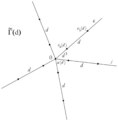
Let us specify the approximation arrangement. The $\delta$’s are placed as sketched on Fig. 1, all dependent on a parameter $d$ in terms of which the limit is performed:

  • there is a $\delta$ coupling with parameter $u(d)$ in the star centre

  • on each halfline there is a $\delta$ interaction with parameter $v_{j}(d)$, where $j$ is the halfline index, at a distance $D(d)$ from the centre (it will turn out in the following that we may choose $D(d)=d^{3}$)

  • furthermore, each halfline supports another $\delta$ interaction with parameter $w_{j}(d)$ at the distance $D(d)+d$ from the centre

Refer to caption
Figure 1: Scheme of a $2n$-parameter approximation

For the sake of brevity we will not indicate the $d$-dependence of the parameters $u,\,v_{j},\,w_{j}$ and the distance $D$ unless necessary. The boundary conditions which the functions $\psi_{1},\ldots,\psi_{n}$ on $\Gamma$ have to satisfy are

$\displaystyle\psi_{1}(0)=\psi_{2}(0)=\cdots=\psi_{n}(0)=:\psi(0)\,,\qquad\sum^{n}_{j=1}\psi_{j}^{\prime}(0_{+})=u\psi(0)$ (24)
$\displaystyle\psi_{j}(D_{+})=\psi_{j}(D_{-})=:\psi_{j}(D)\,,\quad\psi_{j}^{\prime}(D_{+})-\psi_{j}^{\prime}(D_{-})=v_{j}\psi_{j}(D)$ (25)
$\displaystyle\psi_{j}(D+d_{\pm})=:\psi_{j}(D+d)\,,\quad\psi_{j}^{\prime}(D+d_{+})-\psi_{j}^{\prime}(D+d_{-})=w_{j}\psi_{j}(D+d)\,.\phantom{A}$ (26)

Further relations which will in the following serve to determine the parameter dependence on $d$ are obtained from Taylor expansion of the respective wave functions,

$\displaystyle\psi_{j}(D)=\psi_{j}(0)+D\psi_{j}^{\prime}(0_{+})+\mathcal{O}(D^{2})\,,\qquad\psi_{j}^{\prime}(D_{-})=\psi_{j}^{\prime}(0_{+})+\mathcal{O}(D)\,,$ (27)
$\displaystyle\psi_{j}(D+d)=\psi_{j}(D)+d\psi_{j}^{\prime}(D_{+})+\mathcal{O}(d^{2})\,,\;\psi_{j}^{\prime}(D+d_{-})=\psi_{j}^{\prime}(D_{+})+\mathcal{O}(d)\phantom{AA}$ (28)

for $j\in\hat{n}$. We need to find relations between the values $\psi_{1}(D+d),\ldots,\psi_{n}(D+d)$ and $\psi_{1}^{\prime}(D+d_{+}),\ldots,\psi_{n}^{\prime}(D+d_{+})$. To this aim we express them first in terms of $\psi(0)$ and $\psi_{j}^{\prime}(0_{+})$. Using the relations (25) and (27) we get

$\displaystyle\psi_{j}^{\prime}(D_{+})$ $\displaystyle=\psi_{j}^{\prime}(0_{+})+\mathcal{O}(D)+v_{j}(\psi_{j}(0)+D\psi_{j}^{\prime}(0_{+})+\mathcal{O}(D^{2}))=$
$\displaystyle=v_{j}\psi(0)+(1+v_{j}D)\psi_{j}^{\prime}(0_{+})+\mathcal{O}(D)+v_{j}\mathcal{O}(D^{2})\,.$

Substituting into the first one of the relations (28) and using  (25) again we find

$$\psi_{j}(D+d)=(1+dv_{j})\psi(0)+\left(D+d(1+v_{j}D)\right)\psi_{j}^{\prime}(0_{+})\\ +\mathcal{O}(D^{2})+d\mathcal{O}(D)+dv_{j}\mathcal{O}(D^{2})+\mathcal{O}(d^{2})\,.$$ (29)

The already obtained expression for $\psi_{j}^{\prime}(D_{+})$ together with the second one of the relations  (28) give

$$\psi_{j}^{\prime}(D+d_{-})=v_{j}\psi(0)+(1+v_{j}D)\psi_{j}^{\prime}(0_{+})+\mathcal{O}(D)+v_{j}\mathcal{O}(D^{2})+\mathcal{O}(d)\,.$$

Substituting from here and (29) into the second one of the relations (26) we get after a simple rearrangement

$$\psi_{j}^{\prime}(D+d_{+})=\left(v_{j}+w_{j}(1+dv_{j})\right)\psi(0)+\left(1+v_{j}D+w_{j}\left(D+d(1+v_{j}D)\right)\right)\psi_{j}^{\prime}(0_{+})\phantom{A}\\ +\mathcal{O}(D)+v_{j}\mathcal{O}(D^{2})+\mathcal{O}(d)+w_{j}\left(\mathcal{O}(D^{2})+d\mathcal{O}(D)+dv_{j}\mathcal{O}(D^{2})+\mathcal{O}(d^{2})\right).$$ (30)

Next we eliminate $\psi_{j}^{\prime}(0_{+})$ (for simplicity we write $\psi_{j}^{\prime}(0)$) from the obtained relations (29) and (30), multiplying them by $1+v_{j}D+w_{j}\left(D+d(1+v_{j}D)\right)$ and $D+d(1+v_{j}D)$, respectively, and subtracting. In the resulting expression the coefficient at $\psi(0)$ equals one,

$$\left(1+v_{j}D+w_{j}\left(D+d(1+v_{j}D)\right)\right)\psi_{j}(D+d)\\ =\psi(0)+\left(D+d(1+v_{j}D)\right)\psi_{j}^{\prime}(D+d_{+})+\mathcal{R}_{j}\,,$$ (31)

with the remainder term

$$\mathcal{R}_{j}:=\left(1+v_{j}D+w_{j}\left(D+d(1+v_{j}D)\right)\right)(\mathcal{O}(D^{2})+d\mathcal{O}(D)+dv_{j}\mathcal{O}(D^{2})+\mathcal{O}(d^{2}))\\ -\left(D+d(1+v_{j}D)\right)\big{(}(\mathcal{O}(D)+v_{j}\mathcal{O}(D^{2})+\mathcal{O}(d)\\ +w_{j}\left(\mathcal{O}(D^{2})+d\mathcal{O}(D)+dv_{j}\mathcal{O}(D^{2})+\mathcal{O}(d^{2})\right)\big{)}\,.$$

So far the edge index has been kept fixed. Subtracting mutually the relations (31) for different values of $j,k\in\mathbb{N}$, we can eliminate $\psi(0)$,

$$\left(1+v_{j}D+w_{j}\left(D+d(1+v_{j}D)\right)\right)\psi_{j}(D+d)\\ -\left(1+v_{k}D+w_{k}\left(D+d(1+v_{k}D)\right)\right)\psi_{k}(D+d)\\ =\left(D+d(1+v_{j}D)\right)\psi_{j}^{\prime}(D+d_{+})-\left(D+d(1+v_{k}D)\right)\psi_{k}^{\prime}(D+d_{+})+\mathcal{R}_{j}-\mathcal{R}_{k}$$ (32)

Returning to the relations (29) and (30) we can eliminate from them $\psi(0)$ in a similar way as above arriving at the relation

$$(1+dv_{j})\psi_{j}^{\prime}(D+d_{+})-\left(v_{j}+w_{j}(1+dv_{j})\right)\psi_{j}(D+d)=\psi_{j}^{\prime}(0)-\tilde{\mathcal{R}}_{j}$$ (33)

with the remainder term

$$\tilde{\mathcal{R}}_{j}:=\left(v_{j}+w_{j}(1+dv_{j})\right)(\mathcal{O}(D^{2})+d\mathcal{O}(D)+dv_{j}\mathcal{O}(D^{2})+\mathcal{O}(d^{2}))-\\ -(1+dv_{j})\left((\mathcal{O}(D)+v_{j}\mathcal{O}(D^{2})+\mathcal{O}(d)+w_{j}\left(\mathcal{O}(D^{2})+d\mathcal{O}(D)+dv_{j}\mathcal{O}(D^{2})+\mathcal{O}(d^{2})\right)\right)\,.$$

Summing the above relations over $j\in\mathbb{N}$ and using  (24) we get

$$\sum^{n}_{j=1}(1+dv_{j})\psi_{j}^{\prime}(D+d_{+})-\sum^{n}_{j=1}\left(v_{j}+w_{j}(1+dv_{j})\right)\psi_{j}(D+d)=u\psi(0)-\sum^{n}_{j=1}\tilde{\mathcal{R}}_{j}\,.$$ (34)

The right-hand side can rewritten using the continuity condition (24) in combination with the relation (31),

$$u\psi(0)=\frac{u}{n}\sum^{n}_{j=1}\psi_{j}(0)=\frac{u}{n}\sum^{n}_{j=1}\big{(}\left(1+v_{j}D+w_{j}\left(D+d(1+v_{j}D)\right)\right)\psi_{j}(D+d)\\ -\left(D+d(1+v_{j}D)\right)\psi_{j}^{\prime}(D+d_{+})+\mathcal{R}_{j}\big{)}\,.$$

This allows us to cast (34) into a form which contains neither $\psi(0)$ nor $\psi_{j}^{\prime}(0)$,

$$\sum^{n}_{j=1}\left(v_{j}+w_{j}(1+dv_{j})+\frac{u}{n}\left(1+v_{j}D+w_{j}\left(D+d(1+v_{j}D)\right)\right)\right)\psi_{j}(D+d)=\\ =\sum^{n}_{j=1}\left(1+dv_{j}+\frac{u}{n}\left(D+d(1+v_{j}D)\right)\right)\psi_{j}^{\prime}(D+d_{+})+\sum^{n}_{j=1}\left(\tilde{\mathcal{R}}_{j}-\frac{u}{n}\mathcal{R}_{j}\right)\,.$$ (35)

The equations (32) and (35) are the sought relations between the function values and derivatives at the sites of the “outer” $\delta$’s with $\psi(0)$ and $\psi_{j}^{\prime}(0)$ eliminated.

In the next step we are going to choose the dependences $D=D(d),\,u=u(d),\,v_{j}=v_{j}(d)$ and $w_{j}=w_{j}(d)$ for $j\in\hat{n}$ in such a way that the limit $d\to 0_{+}$ will yield the ($2n$-parameter family of) boundary conditions (1) satisfying the requirement (2). It appears that a suitable choice is the following one,

$$\begin{split}D(d)&:=d^{3}\\ 1+v_{j}D&=\alpha_{j}d\,,\quad\text{i.e.}\quad v_{j}(d):=-\frac{1}{d^{3}}+\frac{\alpha_{j}}{d^{2}}\\ 1+w_{j}d&=\beta_{j}d\,,\quad\text{i.e.}\quad w_{j}(d):=-\frac{1}{d}+\beta_{j}\\ u(d)&:=\frac{\omega}{d^{4}}\end{split}$$ (36)

Indeed, in such a case the coefficients in (32) acquire the form

$$\begin{split}(1+v_{j}D)(1+w_{j}d)+w_{j}D&=(\alpha_{j}\beta_{j}-1)d^{2}+\beta_{j}d^{3}\,,\\ D+d(1+v_{j}D)&=\alpha_{j}d^{2}+d^{3}\end{split}$$ (37)

and a straightforward computation shows that the remainders are $\mathcal{R}_{j}=d^{2}\mathcal{O}(d)$, hence dividing (32) by $d^{2}$ we arrive at

$$\begin{split}(\alpha_{j}\beta_{j}-1+\beta_{j}d)\psi_{j}(d^{3}+d)-(\alpha_{k}\beta_{k}-1+\beta_{k}d)\psi_{k}(d^{3}+d)\\ =(\alpha_{j}+d)\psi_{j}^{\prime}(d^{3}+d_{+})-(\alpha_{k}+d)\psi_{k}^{\prime}(d^{3}+d_{+})+\mathcal{O}(d)\,.\end{split}$$

Taking the limit $d\to 0_{+}$ we have to realize that the condition $\psi_{j}\in W^{2,2}(\mathbb{R}^{+}),\,j\in\hat{n}$, requires that $\psi_{j}(d)=o(d^{-1/2})$ holds at the halfline endpoint, hence we have

$$(\alpha_{j}\beta_{j}-1)\psi_{j}(0)-(\alpha_{k}\beta_{k}-1)\psi_{k}(0)=\alpha_{j}\psi_{j}^{\prime}(0)-\alpha_{k}\psi_{k}^{\prime}(0)\,,\quad j,k\in\hat{n}\,.$$ (38)

In a similar way we proceed with the equation (35). We employ (37), then a straightforward computation gives for the coefficients at $\psi_{j}(D+d)$ and $\psi_{j}^{\prime}(D+d_{+})$ the following expressions

$\displaystyle v_{j}+w_{j}(1+dv_{j})+\frac{u}{n}\left(1+v_{j}D+w_{j}\left(D+d(1+v_{j}D)\right)\right)$
$\displaystyle\qquad=\left(-\beta_{j}+\frac{\omega}{n}(\alpha_{j}\beta_{j}-1)\right)\frac{1}{d^{2}}+\left(\alpha_{j}\beta_{j}-1+\frac{\omega}{n}\beta_{j}\right)\frac{1}{d}+\beta_{j}\,,$
$\displaystyle 1+dv_{j}+\frac{u}{n}\left(D+d(1+v_{j}D)\right)=\left(-1+\frac{\omega}{n}\alpha_{j}\right)\frac{1}{d^{2}}+\left(\alpha_{j}+\frac{\omega}{n}\right)\frac{1}{d}+1\,,$

and the remainder terms $\tilde{\mathcal{R}}_{j}$ and $\frac{u}{n}\mathcal{R}_{j}$ are both $d^{-2}\mathcal{O}(d)$. We substitute from here to (35), multiply the result by $d^{2}$ and pass to the limit $d\to 0_{+}$; this yields

$$\sum^{n}_{j=1}\left(-\beta_{j}+\frac{\omega}{n}(\alpha_{j}\beta_{j}-1)\right)\psi_{j}(0)=\sum^{n}_{j=1}\left(-1+\frac{\omega}{n}\alpha_{j}\right)\psi_{j}^{\prime}(0)\,,\quad j\in\hat{n}\,.$$ (39)

The relations (38) and (39) are the sought boundary conditions. It remains to express them as (1) and to find relations between the parameters contained in them to those of (21). The matrix form of (38) and (39) looks as follows,

$$\left(\begin{array}[]{cccc}\alpha_{1}\beta_{1}-1&-(\alpha_{2}\beta_{2}-1)&\cdots&0\\ \vdots&&\ddots&\\ \alpha_{1}\beta_{1}-1&0&\cdots&-(\alpha_{n}\beta_{n}-1)\\ \tilde{\gamma}_{1}&\tilde{\gamma}_{2}&\cdots&\tilde{\gamma}_{n}\end{array}\right)\Psi(0)+\left(\begin{array}[]{cccc}-\alpha_{1}&\alpha_{2}&\cdots&0\\ \vdots&&\ddots&\\ -\alpha_{1}&0&\cdots&\alpha_{n}\\ \tilde{\tau}_{1}&\tilde{\tau}_{2}&\cdots&\tilde{\tau}_{n}\end{array}\right)\Psi^{\prime}(0)=0\,,$$ (40)

where $\tilde{\gamma}_{j}:=\frac{\omega}{n}(\alpha_{j}\beta_{j}-1)-\beta_{j}$ and $\tilde{\tau}_{j}:=1-\frac{\omega}{n}\alpha_{j}$. We know that the corresponding matrix of (3) is given by $U=-(A+\mathrm{i}B)^{-1}\cdot(A-\mathrm{i}B)$, its matrix element being

$\displaystyle U_{jj}=$ $\displaystyle\frac{2\mathrm{i}}{(\alpha_{j}\beta_{j}-1-\mathrm{i}\alpha_{j})^{2}\left(\sum^{n}_{l=1}\frac{\beta_{l}(\alpha_{l}\beta_{l}-1)+\alpha_{l}}{(\alpha_{l}\beta_{l}-1)^{2}+\alpha_{l}^{2}}-\omega+\mathrm{i}\sum^{n}_{l=1}\frac{1}{(\alpha_{l}\beta_{l}-1)^{2}+\alpha_{l}^{2}}\right)}$
$\displaystyle\quad-\frac{\alpha_{j}\beta_{j}-1+\mathrm{i}\alpha_{j}}{\alpha_{j}\beta_{j}-1-\mathrm{i}\alpha_{j}}$

and

$$U_{jk}=\frac{2\mathrm{i}}{(\alpha_{j}\beta_{j}-1-\mathrm{i}\alpha_{j})(\alpha_{k}\beta_{k}-1-\mathrm{i}\alpha_{k})\left(\sum^{n}_{l=1}\frac{\beta_{l}(\alpha_{l}\beta_{l}-1)+\alpha_{l}}{(\alpha_{l}\beta_{l}-1)^{2}+\alpha_{l}^{2}}-\omega+\mathrm{i}\sum^{n}_{l=1}\frac{1}{(\alpha_{l}\beta_{l}-1)^{2}+\alpha_{l}^{2}}\right)}$$

for $j\neq k$. If the latter should correspond to  (21), it is sufficient to require

$$|\alpha_{1}\beta_{1}-1-\mathrm{i}\alpha_{1}|=1$$ (41)

and to set

$\displaystyle\sum^{n}_{l=1}\frac{\beta_{l}(\alpha_{l}\beta_{l}-1)+\alpha_{l}}{(\alpha_{l}\beta_{l}-1)^{2}+\alpha_{l}^{2}}-\omega=\rho\,,$ (42)
$\displaystyle\alpha_{j}\beta_{j}-1=c_{j}\,,\qquad-\alpha_{j}=t_{j}\,.$ (43)

For $\alpha_{1}=0$ the condition (41) is satified trivially, while for a nonzero value it is equivalent to $\alpha_{1}\left(\alpha_{1}(\beta_{1}^{2}+1)-2\beta_{1}\right)=0$, in other words we have to put

$$\alpha_{1}=\frac{2\beta_{1}}{\beta_{1}^{2}+1}\,.$$

In this way we have eliminated the parameter $\alpha_{1}$, and just $2n$ of them is left. The correspondence between the $2n$-tuples $\beta_{1},\beta_{2},\beta_{3},\ldots\beta_{n},\alpha_{2},\alpha_{3},\ldots,\alpha_{n},\omega$ and $\theta,c_{2},c_{3},\ldots c_{n},t_{2},t_{3},\ldots,t_{n},\rho$ looks as follows:

  • $\beta_{1}\longleftrightarrow\theta$: they are related by $\frac{\beta_{1}-\mathrm{i}}{\beta_{1}+\mathrm{i}}=\mathrm{e}^{\mathrm{i}\theta}$

  • $\alpha_{j},\beta_{j}\longleftrightarrow c_{j},t_{j}$, $j\in\{2,\ldots,n\}$: see (43),

  • $\omega\longleftrightarrow\rho$: see (42).

In what follows we will work with $\beta_{1},\beta_{2},\beta_{3},\ldots\beta_{n},\alpha_{2},\alpha_{3},\ldots\alpha_{n},\omega$, for simplicity we will use also $\alpha_{1}$ remembering that it is determined by $\beta_{1}$ and the relation (41).

4 Norm-resolvent convergence

The approximation worked out in the previous section was in the spirit of [16, 27] being expressed in terms of boundary conditions. One asks naturally what can be said about the relation between the corresponding operators. We denote the Hamiltonian with the coupling (40) in centre of the star as $H^{\omega,\vec{\alpha},\vec{\beta}}$, and $H^{u,\vec{v},\vec{w}}(d)$ will be the approximating family constructed above, with a pair of $\delta$ interactions added at each halfline. Our aim here is to demonstrate the following claim.

Theorem 4.1.

Let $u,\,v_{j},\,w_{j},\;j\in\hat{n}$, depend on $d$ according to (36), i.e.

$$u(d)=\frac{\omega}{d^{4}}\,,\quad v_{j}(d)=-\frac{1}{d^{3}}+\frac{\alpha_{j}}{d^{2}}\,,\quad w_{j}(d)=-\frac{1}{d}+\beta_{j}\,.$$

Then $H^{u,\vec{v},\vec{w}}(d)$ converges to $H^{\omega,\vec{\alpha},\vec{\beta}}$ in the norm-resolvent sense as $d\to 0_{+}$.

Proof 4.2.

We have to compare the resolvents $R_{H^{u,\vec{v},\vec{w}}(d)}(k^{2})$ and $R_{H^{\omega,\vec{\alpha},\vec{\beta}}}(k^{2})$ of the two operators for $k^{2}$ in the resolvent set. It is clearly sufficient to check the convergence in the Hilbert-Schmidt norm,

$$\left\|R_{H^{u,\vec{v},\vec{w}}(d)}(k^{2})-R_{H^{\omega,\vec{\alpha},\vec{\beta}}}(k^{2})\right\|_{2}\to 0_{+}\quad\text{ as }\>d\longrightarrow 0_{+}\,,$$

in other words, to show that the difference of the corresponding resolvent kernels denoted as $\mathcal{G}^{u,\vec{v},\vec{w}}_{k}$ and $\mathcal{G}^{\omega,\vec{\alpha},\vec{\beta}}_{k}$, respectively, tends to zero in $L^{2}((\mathbb{R}^{+})^{2n})$. Recall that these jernels, or Green functions, are in our case $n\times n$ matrix functions.

Let us construct first $\mathcal{G}^{\omega,\vec{\alpha},\vec{\beta}}_{k}$ for the star-graph Hamiltonian referring to the condition (1) in the centre. We begin with $n$ independent halflines with Dirichlet condition at its endpoints; Green’s function for each of them is well-known to be

$$\mathcal{G}_{\mathrm{i}\kappa}(x,y)=\frac{\sinh\kappa x_{<}\>\mathrm{e}^{-\kappa x_{>}}}{\kappa}\,,$$

where $x_{<}:=\min\{x,y\},\>x_{>}:=\max\{x,y\}$, and we put $\mathrm{i}\kappa=k$ assuming $\mathrm{Re\,}\kappa>0$. The sought Green’s function is then given by Krein’s formula [4, App. A],

$$R_{H^{A,B}}(k^{2})=R_{H}(k^{2})+\sum^{n}_{j,l=1}\lambda_{jl}(k^{2})\left(\phi_{l}\left(\overline{k^{2}}\right),\cdot\right)_{L^{2}((\mathbb{R}^{+})^{n})}\phi_{j}(k^{2})\,,$$ (44)

where $R_{H}(k^{2})$ acts on each halfline as an integral operator with the kernel $\mathcal{G}_{\kappa}$ and for $\phi_{j}(k^{2})$ one can choose any elements of the deficiency subspaces of the largest common restriction; we will work with $\left(\phi_{j}(k^{2})(x)\right)_{m}=\delta_{jm}\mathrm{e}^{-\kappa x}$.

To find the coefficients $\lambda_{jl}(k^{2})$ we apply  (44) to an arbitrary $\Psi\in\bigoplus_{j=1}^{n}L^{2}(\mathbb{R}^{+})$ and denote the components of the resulting vector as $h_{j}$; it yields

$$h_{j}(x_{j})=\int^{+\infty}_{0}\mathcal{G}_{\mathrm{i}\kappa}(x,y_{j})\psi_{j}(y_{j})\mathrm{d}y_{j}+\sum^{n}_{l=1}\lambda_{jl}(k^{2})\int^{+\infty}_{0}\\ e^{-\kappa y_{l}}\psi_{l}(y_{l})\mathrm{d}y_{l}\cdot\mathrm{e}^{-\kappa x_{j}}\,.$$

These functions have to satisfy the boundary conditions in the centre,

$$\sum^{n}_{m=1}A_{jm}h_{m}(0)+\sum^{n}_{m=1}B_{jm}h_{m}^{\prime}(0)=0\quad\text{for all }\;j\in\hat{n}\,.$$ (45)

Using the explicit form of $\mathcal{G}_{\mathrm{i}\kappa}(x,y)$ and $\left.\frac{\partial\mathcal{G}_{\kappa}(x_{m},y_{m})}{\partial x_{m}}\right|_{x_{m}=0}=\mathrm{e}^{-\kappa y_{m}}$ we find

$$h_{m}(0)=\sum^{n}_{l=1}\lambda_{ml}(k^{2})\int^{+\infty}_{0}\mathrm{e}^{-\kappa y_{l}}\psi_{l}(y_{l})\mathrm{d}y_{l}$$ (46)

and

$$h_{m}^{\prime}(0)=\int^{+\infty}_{0}\mathrm{e}^{-\kappa y_{m}}\psi_{m}(y_{m})\mathrm{d}y_{m}-\kappa\sum^{n}_{l=1}\lambda_{ml}(k^{2})\int^{+\infty}_{0}\mathrm{e}^{-\kappa y_{l}}\psi_{l}(y_{l})\mathrm{d}y_{l}\,.$$ (47)

Substituting from these relations into (45) we get a system of equations,

$$\sum^{n}_{l=1}\int^{+\infty}_{0}\left(\sum^{n}_{m=1}A_{jm}\lambda_{ml}(k^{2})+B_{jl}-\kappa\sum^{n}_{m=1}B_{jm}\lambda_{ml}(k^{2})\right)\mathrm{e}^{-\kappa y_{l}}\psi_{l}(y_{l})\mathrm{d}y_{l}=0\,,$$

with $j\in\hat{n}$. We require that the left-hand side vanishes for any $\psi_{1},\psi_{2},\ldots,\psi_{n}$; this yields the condition $A\Lambda+B-\kappa B\Lambda=0$. From here it is easy to find the coefficients $\lambda_{jl}(k^{2})$: we have $(A-\kappa B)\Lambda=-B$, and therefore

$$\lambda_{jl}(k^{2})=-\left[(A-\kappa B)^{-1}B\right]_{jl}\,.$$

Notice that the matrix $A-\kappa B$ is regular in view of the first conditions in (2); since $A,\,B$ are real and $\mathrm{Im\,}\kappa\neq 0$, the requirement $\mathrm{rank}(A,B)=n$ implies that we have also $\mathrm{rank}(A-\kappa B)=n$.

Let us now concentrate on the class of couplings for which we established in the previous section the boundary condition convergence. In this case $A-\kappa B$ equals

$$\left(\begin{array}[]{cccc}\alpha_{1}(\beta_{1}+\kappa)-1&-(\alpha_{2}(\beta_{2}+\kappa)-1)&\cdots&0\\ \vdots&&\ddots&\\ \alpha_{1}(\beta_{1}+\kappa)-1&0&\cdots&-(\alpha_{n}(\beta_{n}+\kappa)-1)\\ (\beta_{1}+\kappa)\left(\frac{\omega}{n}\alpha_{1}-1\right)-\frac{\omega}{n}&(\beta_{2}+\kappa)\left(\frac{\omega}{n}\alpha_{2}-1\right)-\frac{\omega}{n}&\cdots&(\beta_{n}+\kappa)\left(\frac{\omega}{n}\alpha_{n}-1\right)-\frac{\omega}{n}\end{array}\right),$$

and a tedious by straightforward computation yields an explicit form of the matrix $-(A-\kappa B)^{-1}B$, namely

$$\begin{split}\left[-(A-\kappa B)^{-1}B\right]_{jl}=&\frac{1}{\omega-\sum^{n}_{m=1}\frac{\beta_{m}+\kappa}{\alpha_{m}(\beta_{m}+\kappa)-1}}\cdot\frac{1}{(\alpha_{j}(\beta_{j}+\kappa)-1)(\alpha_{l}(\beta_{l}+\kappa)-1)}\\ &\hskip 199.16928pt\text{ for }j\neq l\,,\\ \left[-(A-\kappa B)^{-1}B\right]_{jj}=&\frac{1}{\omega-\sum^{n}_{m=1}\frac{\beta_{m}+\kappa}{\alpha_{m}(\beta_{m}+\kappa)-1}}\cdot\frac{1}{(\alpha_{j}(\beta_{j}+\kappa)-1)^{2}}+\frac{\alpha_{j}}{\alpha_{j}(\beta_{j}+\kappa)-1}\,.\end{split}$$

In this way we get the Green function $\mathcal{G}^{\omega,\vec{\alpha},\vec{\beta}}_{\mathrm{i}\kappa}$. As we have mentioned above, it is an $n\times n$ matrix-valued function the ($j,l$)-th element of which is given by

$$\begin{split}\mathcal{G}^{\omega,\vec{\alpha},\vec{\beta}}_{\mathrm{i}\kappa,jl}(x,y)=&\delta_{jl}\left(\frac{\sinh\kappa x_{<}\>\mathrm{e}^{-\kappa x_{>}}}{\kappa}+\mathrm{e}^{-\kappa(x+y)}\frac{\alpha_{j}}{\alpha_{j}(\beta_{j}+\kappa)-1}\right)+\\ +&\frac{1}{\omega-\sum^{n}_{m=1}\frac{\beta_{m}+\kappa}{\alpha_{m}(\beta_{m}+\kappa)-1}}\cdot\frac{1}{(\alpha_{j}(\beta_{j}+\kappa)-1)(\alpha_{l}(\beta_{l}+\kappa)-1)}\ \mathrm{e}^{-\kappa x}\mathrm{e}^{-\kappa y}\,;\end{split}$$

we use the convention that $x$ is from the $j$-th halfline and $y$ from the $l$-th one.

Next we will pass to resolvent construction for the approximating family of operators $H^{u,\vec{v},\vec{w}}(d)$. As a starting point we consider $n$ independent halflines with Dirichlet endpoints; we know that the appropriate Green’s function is $\mathcal{G}_{\mathrm{i}\kappa}(x,y)=\kappa^{-1}\sinh\kappa x_{<}\mathrm{e}^{-\kappa x_{>}}$. The sought resolvent kernel will be then found in several steps. Each of them represents an application of Krein’s formula. First we add the $\delta$ interaction with the parameter $v$ at the distance $d^{3}$ from the endpoint, then another one with the parameter $w$ at the distance $d+d^{3}$, again from the endpoint. This is done on each halfline separately. In the final step we find Green’s function for the star in which the Dirichlet ends are replaced by the $\delta$ coupling with the parameter $u$. That will require, of course, to distinguish the halflines by their indices.

The first step is rather standard [19] and resulting Green function is

$$\mathcal{G}_{\mathrm{i}\kappa}^{v}(x,y)=\mathcal{G}_{\mathrm{i}\kappa}(x,y)-\frac{v}{1+v\cdot\mathcal{G}_{\mathrm{i}\kappa}(d^{3},d^{3})}\ \mathcal{G}_{\mathrm{i}\kappa}(y,d^{3})\ \mathcal{G}_{\mathrm{i}\kappa}(x,d^{3})\,.$$ (48)

Adding another $\delta$ interaction at the distance $d$ from the previous one we seek the kernel in the form $R^{v,w}(k^{2})=R^{v}(k^{2})+\lambda(k^{2})\big{(}\phi(\overline{k^{2}}),\cdot\big{)}\phi(k^{2})$ where the first term is $R^{v}(k^{2}):=\mathcal{G}_{\mathrm{i}\kappa}^{v}$ and the deficiency-subspace element $\phi(k^{2})$ is chosen as

$$\phi(k^{2})(x):=\mathcal{G}^{v}_{\mathrm{i}\kappa}(x,d+d^{3})\,.$$

We apply this Ansatz to any $\psi\in L^{2}(\mathbb{R}^{+})$ and denote $h:=R^{v,w}(k^{2})\psi$. It is easy to check that $\overline{\mathcal{G}^{v}_{\mathrm{i}\bar{\kappa}}(x,y)}=\mathcal{G}^{v}_{\mathrm{i}\kappa}(x,y)$, hence we can write $h$ explicitly as

$$h(x)=\int^{+\infty}_{0}\mathcal{G}^{v}_{\mathrm{i}\kappa}(x,y)\psi(y)\,\mathrm{d}y+\lambda(k^{2})\int^{+\infty}_{0}\mathcal{G}^{v}_{\mathrm{i}\kappa}(y,d+d^{3})\psi(y)\,\mathrm{d}y\cdot\mathcal{G}^{v}_{\mathrm{i}\kappa}(x,d+d^{3})\,.$$

By definition this function this function belongs to the domain of the operator with two $\delta$ interactions, in particular, it has to satisfy the boundary conditions

$$\displaystyle h({d+d^{3}}_{+})=h({d+d^{3}}_{-})=:h(d+d^{3})\,,$$ (49)
$$\displaystyle h^{\prime}({d+d^{3}}_{+})-h^{\prime}({d+d^{3}}_{-})=w\cdot h(d+d^{3})\,.$$ (50)

Green’s function continuity implies (49). Furthermore, we have

$$h^{\prime}(x)=\int^{+\infty}_{0}\frac{\partial\mathcal{G}^{v}_{\mathrm{i}\kappa}(x,y)}{\partial x}\psi(y)\,\mathrm{d}y+\lambda(k^{2})\int^{+\infty}_{0}\mathcal{G}^{v}_{\mathrm{i}\kappa}(y,d+d^{3})\psi(y)\,\mathrm{d}y\cdot\frac{\partial\mathcal{G}^{v}_{\mathrm{i}\kappa}(x,d+d^{3})}{\partial x}\,,$$

which allows us to express $h^{\prime}(d+d^{3}_{+})-h^{\prime}(d+d^{3}_{-})$. The first term obviously does not contribute to the difference, while the contribution of the second one simplifies in view of $\left.\frac{\partial\mathcal{G}(x,y)}{\partial x}\right|_{y_{+}}-\left.\frac{\partial\mathcal{G}(x,y)}{\partial x}\right|_{y_{-}}=-1$ to the form

$$h^{\prime}(d+d^{3}_{+})-h^{\prime}(d+d^{3}_{-})=-\lambda(k^{2})\int^{+\infty}_{0}\mathcal{G}^{v}_{\mathrm{i}\kappa}(y,d+d^{3})\psi(y)\,\mathrm{d}y\,.$$

To satisfy (50) the coefficient $\lambda(k^{2})$ must obey the condition

$$\int^{+\infty}_{0}\left[\lambda(k^{2})+w+w\lambda(k^{2})\mathcal{G}^{v}_{\mathrm{i}\kappa}(d+d^{3},d+d^{3})\right]\mathcal{G}^{v}_{\mathrm{i}\kappa}(y,d+d^{3})\psi(y)\,\mathrm{d}y=0$$

for any $\psi\in L^{2}(\mathbb{R}^{+})$, where we have taken Green’s function symmetry with respect to the argument interchange into account. Consequently, the square bracket has to vanish and we get the formula for the kernel with two $\delta$ interactions,

$$\mathcal{G}_{\mathrm{i}\kappa}^{v,w}(x,y)=\mathcal{G}^{v}_{\mathrm{i}\kappa}(x,y)-\frac{w}{1+w\cdot\mathcal{G}^{v}_{\mathrm{i}\kappa}(d+d^{3},d+d^{3})}\ \mathcal{G}^{v}_{\mathrm{i}\kappa}(y,d+d^{3})\ \mathcal{G}^{v}_{\mathrm{i}\kappa}(x,d+d^{3})\,.$$ (51)

The remaining step will be more complicated because we are going to introduce a coupling between different halflines working this with matrix-valued functions. Our tool will be again Krein’s formula which now takes the form

$$R_{H^{u,\vec{v},\vec{w}}}(k^{2})=R_{H^{\vec{v},\vec{w}}}(k^{2})+\sum^{n}_{j,l=1}\lambda_{jl}(k^{2})\left(\phi_{l}(\overline{k^{2}}),\cdot\right)_{L^{2}((\mathbb{R}^{+})^{n})}\cdot\phi_{j}(k^{2})\,,$$

where the functions $\phi_{j}(k^{2})$ will be chosen as

$$\left(\phi_{j}(k^{2})(x)\right)_{m}=\delta_{jm}\cdot\left.\frac{\partial\mathcal{G}^{v_{m},w_{m}}_{\mathrm{i}\kappa}(x,y)}{\partial y}\right|_{y=0}\,.$$

We apply this Ansatz to an arbitrary $\Psi=\{\psi_{1},\ldots,\psi_{n}\}^{T}$ and denote the elements of the resulting vector as $h_{j}$, explicitly

$$\begin{split}h_{j}(x)=&\int^{+\infty}_{0}\mathcal{G}^{v_{j},w_{j}}_{\mathrm{i}\kappa}(x,y)\psi_{j}(y)\mathrm{d}y\ +\\ +&\sum^{n}_{l=1}\lambda_{jl}(k^{2})\int^{+\infty}_{0}\left.\frac{\partial\mathcal{G}^{v_{l},w_{l}}_{\mathrm{i}\kappa}(x,y)}{\partial x}\right|_{x=0}\psi_{l}(y)\,\mathrm{d}y\cdot\left.\frac{\partial\mathcal{G}^{v_{j},w_{j}}_{\mathrm{i}\kappa}(x,y)}{\partial y}\right|_{y=0}\,.\end{split}$$ (52)

where we have used Green’s function symmetry and the fact that its complex conjugation is equivalent to switching from $\kappa$ to $\bar{\kappa}$. As before the functions $h_{1},h_{2},\ldots,h_{n}$ have to satisfy the boundary conditions expressing the $\delta$ coupling in the star centre,

$$\displaystyle h_{1}(0)=h_{2}(0)=\cdots=h_{n}(0)=:h(0)\,,$$ (53)
$$\displaystyle h_{1}^{\prime}(0)+h_{2}^{\prime}(0)+\cdots+h_{n}^{\prime}(0)=u\cdot h(0)\,,$$ (54)

for any $\psi_{1},\ldots,\psi_{n}\in L^{2}(\mathbb{R}^{+})$. Let us first express $h_{j}(0)$. The first term in the above expression does not contribute since $\mathcal{G}^{v_{j},w_{j}}_{\mathrm{i}\kappa}(0,y)=\mathcal{G}_{\mathrm{i}\kappa}^{v}(0,y)=0$. The second one contains the value of Green’s function derivative which can be expressed using (51),

$\displaystyle\left.\frac{\partial\mathcal{G}^{v_{j},w_{j}}_{\mathrm{i}\kappa}(x,y)}{\partial y}\right|_{y=0}$ $\displaystyle=\left.\frac{\partial\mathcal{G}^{v}_{\mathrm{i}\kappa}(x,y)}{\partial y}\right|_{y=0}$
$\displaystyle-$ $\displaystyle\frac{w}{1+w\cdot\mathcal{G}^{v}_{\mathrm{i}\kappa}(d+d^{3},d+d^{3})}\cdot\left.\frac{\partial\mathcal{G}^{v}_{\mathrm{i}\kappa}(y,d+d^{3})}{\partial y}\right|_{y=0}\cdot\mathcal{G}^{v}_{\mathrm{i}\kappa}(x,d+d^{3})\,.$

The first term is obtained from (48) together with the explicit form of the “free” kernel $\mathcal{G}_{\mathrm{i}\kappa}(x,y)$: we have

$$\left.\frac{\partial\mathcal{G}^{v}_{\mathrm{i}\kappa}(x,y)}{\partial y}\right|_{y=0}=\mathrm{e}^{-\kappa x}-\frac{v}{1+v\cdot\mathcal{G}_{\mathrm{i}\kappa}(d^{3},d^{3})}\ \mathrm{e}^{-\kappa d^{3}}\ \cdot\mathcal{G}_{\mathrm{i}\kappa}(x,d^{3})\,,$$

in particular, $\left.\frac{\partial\mathcal{G}^{v}_{\mathrm{i}\kappa}(x,y)}{\partial y}\right|_{x=y=0}=1$. This further implies

$$\left.\frac{\partial\mathcal{G}^{v_{j},w_{j}}_{\mathrm{i}\kappa}(x,y)}{\partial y}\right|_{y=0}=\mathrm{e}^{-\kappa x}-\frac{v_{j}}{1+v_{j}\cdot\mathcal{G}_{\mathrm{i}\kappa}(d^{3},d^{3})}\ \mathrm{e}^{-\kappa d^{3}}\ \mathcal{G}_{\mathrm{i}\kappa}(x,d^{3})\\ -\frac{w_{j}}{1+w_{j}\cdot\mathcal{G}^{v_{j}}_{\mathrm{i}\kappa}(d+d^{3},d+d^{3})}\cdot\Big{(}\mathrm{e}^{-\kappa(d+d^{3})}\\ -\frac{v_{j}}{1+v_{j}\cdot\mathcal{G}_{\mathrm{i}\kappa}(d^{3},d^{3})}\ \mathrm{e}^{-\kappa d^{3}}\ \mathcal{G}_{\mathrm{i}\kappa}(d+d^{3},d^{3})\Big{)}\cdot\mathcal{G}^{v_{j}}_{\mathrm{i}\kappa}(x,d+d^{3})\,,$$ (55)

in particular, $\left.\frac{\partial\mathcal{G}^{v_{j},w_{j}}_{\mathrm{i}\kappa}(x,y)}{\partial y}\right|_{x=y=0}=1$. Putting these results together, we can simplify the expression for the boundary values $h_{j}(0)$ as follows,

$$h_{j}(0)=\sum^{n}_{l=1}\lambda_{jl}(k^{2})\int^{+\infty}_{0}\left.\frac{\partial\mathcal{G}^{v_{l},w_{l}}_{\mathrm{i}\kappa}(x,y)}{\partial x}\right|_{x=0}\psi_{l}(y)\,\mathrm{d}y\,.$$

Now we can find what is required to fulfill the conditions (53), i.e. $h_{j}(0)=h_{m}(0)$ for all $j,m\in\hat{n}$. This is true provided

$$\sum^{n}_{l=1}\left(\lambda_{jl}(k^{2})-\lambda_{ml}(k^{2})\right)\int^{+\infty}_{0}\left.\frac{\partial\mathcal{G}^{v_{l},w_{l}}_{\mathrm{i}\kappa}(x,y)}{\partial x}\right|_{x=0}\psi_{l}(y)\,\mathrm{d}y=0\,,$$

holds for any $n$-tuple of functions $\psi_{1},\ldots,\psi_{n}\in L^{2}(\mathbb{R}^{+})$ which is possible if

$$\lambda_{jl}(k^{2})=\lambda_{ml}(k^{2})\quad\text{ for all }j,m\in\hat{n},\;l\in\hat{n}\,,$$

thus we can simplify notation writing $\lambda_{l}:=\lambda_{jl}(k^{2})$ for a fixed $l\in\hat{n}$.

Values of the coefficients $\lambda_{1},\ldots,\lambda_{n}$ can be found from the remaining condition (54). To this aim we have to find explicit form of $h_{j}^{\prime}(0)$. It follows from the expression (52) for $h_{j}(x)$ that

$$\begin{split}h_{j}^{\prime}(0)=&\int^{+\infty}_{0}\left.\frac{\partial\mathcal{G}^{v_{j},w_{j}}_{\mathrm{i}\kappa}(x,y)}{\partial x}\right|_{x=0}\psi_{j}(y)\,\mathrm{d}y\ \\ +&\sum^{n}_{l=1}\lambda_{l}\int^{+\infty}_{0}\left.\frac{\partial\mathcal{G}^{v_{l},w_{l}}_{\mathrm{i}\kappa}(x,y)}{\partial x}\right|_{x=0}\psi_{l}(y)\,\mathrm{d}y\cdot\left.\frac{\mathrm{d}}{\mathrm{d}x}\left(\left.\frac{\partial\mathcal{G}^{v_{j},w_{j}}_{\mathrm{i}\kappa}(x,y)}{\partial y}\right|_{y=0}\right)\right|_{x=0}\,,\end{split}$$

The boundary condition (54) then requires that the expression

$$\begin{split}\sum^{n}_{l=1}\int^{+\infty}_{0}\left(1+\lambda_{l}\sum^{n}_{j=1}\left.\frac{\mathrm{d}}{\mathrm{d}x}\left(\left.\frac{\partial\mathcal{G}^{v_{j},w_{j}}_{\mathrm{i}\kappa}(x,y)}{\partial y}\right|_{y=0}\right)\right|_{x=0}-u\cdot\lambda_{l}\right)\\ \cdot\left.\frac{\partial\mathcal{G}^{v_{l},w_{l}}_{\mathrm{i}\kappa}(x,y)}{\partial x}\right|_{x=0}\psi_{l}(y)\,\mathrm{d}y\end{split}$$

vanishes for any $\psi_{1},\ldots,\psi_{n}$, and this in turn yields

$$\lambda_{l}=\left[u-\sum^{n}_{j=1}\left.\frac{\mathrm{d}}{\mathrm{d}x}\left(\left.\frac{\partial\mathcal{G}^{v_{j},w_{j}}_{\mathrm{i}\kappa}(x,y)}{\partial y}\right|_{y=0}\right)\right|_{x=0}\right]^{-1}\quad\text{ for all }l\in\hat{n}$$

showing, in particular, that $\lambda_{l}$ does not depend on $l$, which means that all the coefficients $\lambda_{jl}(k^{2})$ are the same and equal to the right-hand side of the last relation.

Before specifying the expression in the square bracket let us write down the formula for the ($j,l$)-th component of the sought Green function: we have

$$\mathcal{G}^{u,\vec{v},\vec{w}}_{\mathrm{i}\kappa,jl}(x,y)=\delta_{jl}\cdot\mathcal{G}^{v_{j},w_{j}}_{\mathrm{i}\kappa}(x,y)+\frac{\left.\frac{\partial\mathcal{G}^{v_{j},w_{j}}_{\mathrm{i}\kappa}(x,y)}{\partial y}\right|_{y=0}\cdot\left.\frac{\partial\mathcal{G}^{v_{l},w_{l}}_{\mathrm{i}\kappa}(x,y)}{\partial x}\right|_{x=0}}{u-\sum^{n}_{m=1}\left.\frac{\mathrm{d}}{\mathrm{d}x}\left(\left.\frac{\partial\mathcal{G}^{v_{m},w_{m}}_{\mathrm{i}\kappa}(x,y)}{\partial y}\right|_{y=0}\right)\right|_{x=0}}\,.$$ (56)

The first derivative in the numerator was found in (55) and by Green’s function symmetry the other one is given by the same expression, with $y$ replaced by $x$. The same relation allows us to compute $\frac{\mathrm{d}}{\mathrm{d}x}\left(\left.\frac{\partial\mathcal{G}^{v_{m},w_{m}}_{\mathrm{i}\kappa}(x,y)}{\partial y}\right|_{y=0}\right)$, in particular, to evaluate the quantity appearing in the square bracket above,

$$\left.\frac{\mathrm{d}}{\mathrm{d}x}\left(\left.\frac{\partial\mathcal{G}^{v_{m},w_{m}}_{\mathrm{i}\kappa}(x,y)}{\partial y}\right|_{y=0}\right)\right|_{x=0}=-\kappa-\frac{v_{m}}{1+v_{m}\cdot\mathcal{G}_{\mathrm{i}\kappa}(d^{3},d^{3})}\ \mathrm{e}^{-\kappa d^{3}}\ \cdot\mathrm{e}^{-\kappa d^{3}}\\ -\frac{w_{m}}{1+w_{m}\cdot\mathcal{G}^{v_{m}}_{\mathrm{i}\kappa}(d+d^{3},d+d^{3})}\cdot\Big{(}\mathrm{e}^{-\kappa(d+d^{3})}\\ -\frac{v_{m}}{1+v_{m}\cdot\mathcal{G}_{\mathrm{i}\kappa}(d^{3},d^{3})}\ \mathrm{e}^{-\kappa d^{3}}\ \mathcal{G}_{\mathrm{i}\kappa}(d+d^{3},d^{3})\Big{)}^{2}\,.$$ (57)

The relations (56) and (57) together with (55) and its mirror counterpart describe completely Green’s function $\mathcal{G}^{u,\vec{v},\vec{w}}_{\mathrm{i}\kappa}$ of the approximating operators.

After deriving explicit expressions for the resolvent we can pass to our proper goal which is to prove that the matrix-valued kernel $\mathcal{G}^{u,\vec{v},\vec{w}}_{\mathrm{i}\kappa}$ converges to $\mathcal{G}^{\omega,\vec{\alpha},\vec{\beta}}_{\mathrm{i}\kappa}$ as $d\to 0_{+}$ which in terms of their components can be written as

$$\lim_{d\to 0+}\left\|\mathcal{G}^{u,\vec{v},\vec{w}}_{\mathrm{i}\kappa,jl}-\mathcal{G}^{\omega,\vec{\alpha},\vec{\beta}}_{\mathrm{i}\kappa,jl}\right\|_{L^{2}(\mathbb{R}^{+}\times\mathbb{R}^{+})}=0\,.$$

Depending on the values $x,\,y$ the difference $\mathcal{G}^{u,\vec{v},\vec{w}}_{\mathrm{i}\kappa,jl}(x,y)-\mathcal{G}^{\omega,\vec{\alpha},\vec{\beta}}_{\mathrm{i}\kappa,jl}(x,y)$ takes different forms. Notice that one can suppose without loss of generality that $x\leq y$, and therefore there are six different situations to inspect, namely

  • $\;d+d^{3}\leq x\leq y$,

  • $\;d\leq x\leq d+d^{3}\leq y$,

  •  $\;0<x\leq d^{3}$, $d+d^{3}\leq y$,

  • $\;d^{3}\leq x\leq y\leq d+d^{3}$,

  •  $\;0<x\leq d^{3}\leq y\leq d+d^{3}$,

  •  $\;0<x\leq y\leq d^{3}$.

To express the kernel difference we employ Taylor expansion of $\mathcal{G}^{u,\vec{v},\vec{w}}_{\mathrm{i}\kappa,jl}(x,y)$. Let us start with expressions which appear in the formulae repeatedly. The first one is

$$\frac{v_{m}}{1+v_{m}\cdot\mathcal{G}_{\mathrm{i}\kappa}(d^{3},d^{3})}=\frac{-\frac{1}{d^{3}}+\frac{\alpha_{m}}{d^{2}}}{1+\left(-\frac{1}{d^{3}}+\frac{\alpha_{m}}{d^{2}}\right)\cdot\frac{\sinh\kappa d^{3}\>\mathrm{e}^{-\kappa d^{3}}}{\kappa}}=(*)$$

Using $\sinh(x)=x+\mathcal{O}(x^{2})$ and $\mathrm{e}^{x}=1+\mathcal{O}(x)$ we get

$$\frac{\sinh\kappa d^{3}\>\mathrm{e}^{-\kappa d^{3}}}{\kappa}=\frac{(\kappa d^{3}+\mathcal{O}(d^{6}))(1+\mathcal{O}(d^{3}))}{\kappa}=d^{3}(1+\mathcal{O}(d^{3}))\,,$$

and this in turn allows us to express (*) as follows,

$$(*)=-\frac{1}{d^{3}}\cdot\frac{1-\alpha_{m}d}{1+\left(-\frac{1}{d^{3}}+\frac{\alpha_{m}}{d^{2}}\right)\cdot(d^{3}(1+\mathcal{O}(d^{3})))}=-\frac{1}{d^{4}}\cdot\left(\frac{1}{\alpha_{m}}+\mathcal{O}(d)\right)\,.$$

The next frequent expression is $w_{m}\left(1+w_{m}\cdot\mathcal{G}^{v_{m}}_{\mathrm{i}\kappa}(d+d^{3},d+d^{3})\right)^{-1}$. We employ relation (48) with $v=v_{m}$ and the expansion $\mathrm{e}^{x}=1+x+\mathcal{O}(x^{2})$ together with the explicit form of $\mathcal{G}_{\mathrm{i}\kappa}$; this yields after a straightforward computation

$$\mathcal{G}^{v_{m}}_{\mathrm{i}\kappa}(d+d^{3},d+d^{3})=d\left(1-\kappa d-\frac{d}{\alpha_{m}}+\mathcal{O}(d^{2})\right)=\mathcal{G}_{\mathrm{i}\kappa}(d+d^{3},d+d^{3})-\frac{d^{2}}{\alpha_{m}}+\mathcal{O}(d^{3})\,,$$

and therefore

$$\frac{w_{m}}{1+w_{m}\cdot\mathcal{G}^{v_{m}}_{\mathrm{i}\kappa}(d+d^{3},d+d^{3})}=-\frac{1}{d^{2}}\left(\frac{1}{\beta_{m}+\kappa-\frac{1}{\alpha_{m}}}+\mathcal{O}(d)\right)\,.$$

Now we can expand the first term in $\mathcal{G}^{u,\vec{v},\vec{w}}_{\mathrm{i}\kappa,jl}(x,y)$. Using (51) for the parameters $v=v_{j},\,w=w_{j}$ together with the previous result we get

$$\begin{split}&\mathcal{G}_{\mathrm{i}\kappa}^{v_{j},w_{j}}(x,y)=\frac{\sinh\kappa x\>\mathrm{e}^{-\kappa y}}{\kappa}\\ &+\frac{1}{d^{2}}\left(\frac{1}{\beta_{m}+\kappa-\frac{1}{\alpha_{m}}}+\mathcal{O}(d)\right)\ \frac{\sinh\kappa(d+d^{3})\,\mathrm{e}^{-\kappa y}}{\kappa}\ \frac{\sinh\kappa(d+d^{3})\,\mathrm{e}^{-\kappa x}}{\kappa}\\ &=\frac{\sinh\kappa x\>\mathrm{e}^{-\kappa y}}{\kappa}+\frac{1}{\beta_{m}+\kappa-\frac{1}{\alpha_{m}}}\ \mathrm{e}^{-\kappa x}\ \mathrm{e}^{-\kappa y}\>\big{(}1+\mathcal{O}(d)\big{)}\end{split}$$

As for the second term in ((56)), we first expand the derivative in the denominator using $\mathcal{G}_{\mathrm{i}\kappa}(d+d^{3},d^{3})=d^{3}(1+\mathcal{O}(d))$ and (57). A direct computation yields

$$\left.\frac{\mathrm{d}}{\mathrm{d}x}\left(\left.\frac{\partial\mathcal{G}^{v_{m},w_{m}}_{\mathrm{i}\kappa}(x,y)}{\partial y}\right|_{y=0}\right)\right|_{x=0}=\frac{1}{d^{4}}\cdot\left(\frac{\beta_{m}+\kappa}{\alpha_{m}(\beta_{m}+\kappa)-1}+\mathcal{O}(d)\right)\,,$$

and therefore

$$\left(u-\sum^{n}_{m=1}\left.\frac{\mathrm{d}}{\mathrm{d}x}\left(\left.\frac{\partial\mathcal{G}^{v_{m},w_{m}}_{\mathrm{i}\kappa}(x,y)}{\partial y}\right|_{y=0}\right)\right|_{x=0}\right)^{-1}=d^{4}\left(\frac{1}{\omega-\sum^{n}_{m=1}\frac{\beta_{m}+\kappa}{\alpha_{m}(\beta_{m}+\kappa)-1}}+\mathcal{O}(d)\right)\,.$$

Next we expand the derivatives which appear in the numerator using the relation $\mathcal{G}_{\mathrm{i}\kappa}^{v_{m}}(x,d+d^{3})=d(1+\mathcal{O}(d))\,\mathrm{e}^{-\kappa x}$; it gives

$$\left.\frac{\partial\mathcal{G}^{v_{m},w_{m}}_{\mathrm{i}\kappa}(x,y)}{\partial y}\right|_{y=0}=\mathrm{e}^{-\kappa x}-\frac{v_{m}}{1+v_{m}\cdot\mathcal{G}_{\mathrm{i}\kappa}(d^{3},d^{3})}\ \mathrm{e}^{-\kappa d^{3}}\ \mathcal{G}_{\mathrm{i}\kappa}(x,d^{3})-\\ -\frac{w_{m}}{1+w_{m}\cdot\mathcal{G}^{v_{m}}_{\mathrm{i}\kappa}(d+d^{3},d+d^{3})}\ \cdot\\ =\frac{1}{d^{2}}\left(\frac{1}{\alpha_{m}(\beta_{m}+\kappa)-1}+\mathcal{O}(d)\right)\mathrm{e}^{-\kappa x}\,.$$

and the analogous expression for $\left.\frac{\partial\mathcal{G}^{v_{m},w_{m}}_{\mathrm{i}\kappa}(x,y)}{\partial x}\right|_{x=0}$ with $x$ replaced by $y$. This determines the behaviour of the second term at the right-hand side of ((56)) as $d\to 0_{+}$, and for the full kernel $\mathcal{G}^{u,\vec{v},\vec{w}}_{\mathrm{i}\kappa,jl}(x,y)$ we consequently have

$$\begin{split}&\mathcal{G}^{u,\vec{v},\vec{w}}_{\mathrm{i}\kappa,jl}(x,y)=\delta_{jl}\left(\frac{\sinh\kappa x\ \mathrm{e}^{-\kappa y}}{\kappa}+\frac{1+\mathcal{O}(d)}{\beta_{j}+\kappa-\frac{1}{\alpha_{j}}}\>\mathrm{e}^{-\kappa x}\ \mathrm{e}^{-\kappa y}\right)\ \\ &+\left(\frac{1}{\omega-\sum^{n}_{m=1}\frac{\beta_{m}+\kappa}{\alpha_{m}(\beta_{m}+\kappa)-1}}\cdot\frac{1}{\alpha_{j}(\beta_{j}+\kappa)-1}\cdot\frac{1}{\alpha_{l}(\beta_{l}+\kappa)-1}+\mathcal{O}(d)\right)\mathrm{e}^{-\kappa x}\mathrm{e}^{-\kappa y}\,.\end{split}$$

On the other hand, for $x\leq y$ we have

$$\begin{split}\mathcal{G}^{\omega,\vec{\alpha},\vec{\beta}}_{\mathrm{i}\kappa,jl}(x,y)=&\delta_{jl}\left(\frac{\sinh\kappa x\ \mathrm{e}^{-\kappa y}}{\kappa}+\mathrm{e}^{-\kappa(x+y)}\frac{\alpha_{j}}{\alpha_{j}(\beta_{j}+\kappa)-1}\right)+\\ +&\frac{1}{\omega-\sum^{n}_{m=1}\frac{\beta_{m}+\kappa}{\alpha_{m}(\beta_{m}+\kappa)-1}}\cdot\frac{1}{(\alpha_{j}(\beta_{j}+\kappa)-1)(\alpha_{l}(\beta_{l}+\kappa)-1)}\ \mathrm{e}^{-\kappa x}\mathrm{e}^{-\kappa y}\,,\end{split}$$

hence the Green function difference satisfies

$$\mathcal{G}^{u,\vec{v},\vec{w}}_{\mathrm{i}\kappa,jl}(x,y)-\mathcal{G}^{\omega,\vec{\alpha},\vec{\beta}}_{\mathrm{i}\kappa,jl}(x,y)=\mathcal{O}(d)\>\mathrm{e}^{-\kappa x}\mathrm{e}^{-\kappa y}\quad\textrm{as }\>d\to 0_{+}\,.$$

The same estimate is obviously valid also for $d<y<x$, hence there is a constant $K$ independent of $d,\,x$ and $y$ such that

$$\left|\mathcal{G}^{u,\vec{v},\vec{w}}_{\mathrm{i}\kappa,jl}(x,y)-\mathcal{G}^{\omega,\vec{\alpha},\vec{\beta}}_{\mathrm{i}\kappa,jl}(x,y)\right|<K\,d\>\mathrm{e}^{-\kappa x}\mathrm{e}^{-\kappa y}$$ (58)

holds for all $d<1,\>x\geq d+d^{3}$ and $y\geq d+d^{3}$. Now we are in position to estimate the Hilbert-Schmidt norm of the resolvent difference for the operators $H^{\omega,\vec{\alpha},\vec{\beta}}$ and $H^{u,\vec{v},\vec{w}}(d)$ which can be written explicitly as follows,

$$\begin{split}\left\|R_{H^{u,\vec{v},\vec{w}}(d)}(k^{2})-\right.&\left.R_{H^{\omega,\vec{\alpha},\vec{\beta}}}\right\|_{2}^{2}=\sum^{n}_{j,l=1}\int^{+\infty}_{0}\int^{+\infty}_{0}\left|\mathcal{G}^{u,\vec{v},\vec{w}}_{\mathrm{i}\kappa,jl}(x,y)-\mathcal{G}^{\omega,\vec{\alpha},\vec{\beta}}_{\mathrm{i}\kappa,jl}(x,y)\right|^{2}\,\mathrm{d}x\mathrm{d}y\\ =\sum^{n}_{j,l=1}&\left(\int^{+\infty}_{d+d^{3}}\int^{+\infty}_{d+d^{3}}\left|\mathcal{G}^{u,\vec{v},\vec{w}}_{\mathrm{i}\kappa,jl}(x,y)-\mathcal{G}^{\omega,\vec{\alpha},\vec{\beta}}_{\mathrm{i}\kappa,jl}(x,y)\right|^{2}\,\mathrm{d}x\mathrm{d}y\right.\\ &+\int^{d+d^{3}}_{d^{3}}\int^{+\infty}_{d+d^{3}}\left|\mathcal{G}^{u,\vec{v},\vec{w}}_{\mathrm{i}\kappa,jl}(x,y)-\mathcal{G}^{\omega,\vec{\alpha},\vec{\beta}}_{\mathrm{i}\kappa,jl}(x,y)\right|^{2}\,\mathrm{d}x\mathrm{d}y\\ &+\int^{+\infty}_{d+d^{3}}\int^{d+d^{3}}_{d^{3}}\left|\mathcal{G}^{u,\vec{v},\vec{w}}_{\mathrm{i}\kappa,jl}(x,y)-\mathcal{G}^{\omega,\vec{\alpha},\vec{\beta}}_{\mathrm{i}\kappa,jl}(x,y)\right|^{2}\,\mathrm{d}x\mathrm{d}y\\ &+\int^{d^{3}}_{0}\int^{+\infty}_{d+d^{3}}\left|\mathcal{G}^{u,\vec{v},\vec{w}}_{\mathrm{i}\kappa,jl}(x,y)-\mathcal{G}^{\omega,\vec{\alpha},\vec{\beta}}_{\mathrm{i}\kappa,jl}(x,y)\right|^{2}\,\mathrm{d}x\mathrm{d}y\\ &+\int^{+\infty}_{d+d^{3}}\int^{d^{3}}_{0}\left|\mathcal{G}^{u,\vec{v},\vec{w}}_{\mathrm{i}\kappa,jl}(x,y)-\mathcal{G}^{\omega,\vec{\alpha},\vec{\beta}}_{\mathrm{i}\kappa,jl}(x,y)\right|^{2}\,\mathrm{d}x\mathrm{d}y\\ &+\int^{d+d^{3}}_{d^{3}}\int^{d+d^{3}}_{d^{3}}\left|\mathcal{G}^{u,\vec{v},\vec{w}}_{\mathrm{i}\kappa,jl}(x,y)-\mathcal{G}^{\omega,\vec{\alpha},\vec{\beta}}_{\mathrm{i}\kappa,jl}(x,y)\right|^{2}\,\mathrm{d}x\mathrm{d}y\\ &+\int^{d^{3}}_{0}\int^{d+d^{3}}_{d^{3}}\left|\mathcal{G}^{u,\vec{v},\vec{w}}_{\mathrm{i}\kappa,jl}(x,y)-\mathcal{G}^{\omega,\vec{\alpha},\vec{\beta}}_{\mathrm{i}\kappa,jl}(x,y)\right|^{2}\,\mathrm{d}x\mathrm{d}y\\ &+\int^{d+d^{3}}_{d^{3}}\int^{d^{3}}_{0}\left|\mathcal{G}^{u,\vec{v},\vec{w}}_{\mathrm{i}\kappa,jl}(x,y)-\mathcal{G}^{\omega,\vec{\alpha},\vec{\beta}}_{\mathrm{i}\kappa,jl}(x,y)\right|^{2}\,\mathrm{d}x\mathrm{d}y\\ &\left.+\int^{d^{3}}_{0}\int^{d^{3}}_{0}\left|\mathcal{G}^{u,\vec{v},\vec{w}}_{\mathrm{i}\kappa,jl}(x,y)-\mathcal{G}^{\omega,\vec{\alpha},\vec{\beta}}_{\mathrm{i}\kappa,jl}(x,y)\right|^{2}\,\mathrm{d}x\mathrm{d}y\right)\,.\end{split}$$

The inequality (58) makes it possible to estimate the first one of the integrals,

$$\int^{+\infty}_{d+d^{3}}\int^{+\infty}_{d+d^{3}}\left|\mathcal{G}^{u,\vec{v},\vec{w}}_{\mathrm{i}\kappa,jl}(x,y)-\mathcal{G}^{\omega,\vec{\alpha},\vec{\beta}}_{\mathrm{i}\kappa,jl}(x,y)\right|^{2}\,\mathrm{d}x\mathrm{d}y\leq K^{2}d^{2}\>\left(\int^{+\infty}_{d+d^{3}}e^{-2(\mathrm{Re\,}\kappa)x}\,\mathrm{d}x\right)^{2}\\ =K^{2}d^{2}\frac{e^{-2(\mathrm{Re\,}\kappa)(d+d^{3})}}{2\mathrm{Re\,}\kappa}\leq\frac{K^{2}}{2\mathrm{Re\,}\kappa}\>d^{2}\,,$$

and it is obvious from this inequality that for $d\to 0_{+}$ the integral tends to zero for any $j,l\in\hat{n}$. In a similar way one can estimate each of the remaining eight integrals: using Taylor expansions of $\mathcal{G}^{u,\vec{v},\vec{w}}_{\mathrm{i}\kappa,jl}$ we get a bound for the integrand which shows that the integral vanishes as $d\to 0_{+}$. Since the argument repeats the procedure described above, we skip the details. Putting all this together, we conclude that

$$\lim_{d\to 0_{+}}\left\|R_{H^{u,\vec{v},\vec{w}}(d)}(k^{2})-R_{H^{\omega,\vec{\alpha},\vec{\beta}}}\right\|_{2}^{2}=0\,,$$

and therefore the resolvent difference tends to zero in Hilbert-Schmidt norm as $d\to 0_{+}$ which is what we set up to demonstrate.

5 Approximations with added edges

We have seen that a CS–type scheme can produce a $2n$-parameter family of (self-adjoint) couplings out of the whole set depending on $n^{2}$ real numbers. To get a wider class we have to add to the star graph $\Gamma$ not only vertices but edges as well.

5.1 Admissible couplings

The first question naturally is how many parameters can be achieved in this way. An upper bound on this number is given by the following statement.

Proposition 5.1.

Let $\Gamma$ be a star graph with $n$ semi-infinite edges and denote by $\left\{\tilde{\Gamma}(d):\>d\in\mathbb{R}^{+}\right\}$ a family of graphs obtained from $\Gamma$ by adding finite edges connecting pairwise the halflines; their number may be arbitrary finite but independent of $d$. Suppose that $\tilde{\Gamma}(d)$ supports only $\delta$ couplings and $\delta$ interactions, their number again independent of $d$, and that the distances between all their sites are $\mathcal{O}(d)$ as $d\to 0_{+}$. Suppose that a family of functions $\Psi_{d}\in W^{2,2}\left(\Gamma\setminus(\{c\}\cup V_{d})\right)$, where $c$ is the centre of $\Gamma$, and $V_{d}$ is the set of the vertices added on the halflines, satisfies the conditions (4) with $d$-dependent parameters, and that it converges to $\Psi\in W^{2,2}\left(\Gamma\setminus\{c\}\right)$ which obeys the condition (1) with some $A,\,B$ satisfying the requirements (2). The family of the conditions (1) which can be obtained in this way has real-valued coefficients, $A,B\in\mathbb{R}^{n,n}$, depending thus on at most ${n+1\choose 2}$ parameters.

Proof 5.2.

The $\delta$ coupling in the centre of $\tilde{\Gamma}(d)$, identified with centre of $\Gamma$, is expressed by the conditions (4). For any $j\in\hat{n}$ we denote by $d_{j}$ the coordinate of the most distant point on the $j$-th halfline which supports either a $\delta$ interaction or a $\delta$ coupling at the endpoint of an added edge. We arrange the function values at these points into the $n$-tuple $\Psi(d)$, and similarly $\Psi^{\prime}(d_{+})$ is the $n$-tuple of right derivatives. Let us stress that this a symbolic notation; the elements are $\psi_{j}(d_{j})$ and $\psi^{\prime}_{j}(d_{j+})$, respectively.

As in the proof of Proposition 3.1 we can use (4) to express these quantities through the common value $\psi(0)$ and the right derivatives $\Psi^{\prime}(0_{+})$ at the origin

$\displaystyle M_{1}(d)\Psi(d)$ $\displaystyle=$ $\displaystyle\psi(0)\cdot m_{2}(d)+M_{3}(d)\Psi^{\prime}(0)+\mathcal{R}(d)\,,$
$\displaystyle N_{1}(d)\Psi^{\prime}(d_{+})$ $\displaystyle=$ $\displaystyle\psi(0)\cdot n_{2}(d)+N_{3}(d)\Psi^{\prime}(0)+\tilde{\mathcal{R}}(d)$

for some $M_{1},M_{3},N_{1},N_{3}:\mathbb{R}^{+}\to\mathbb{R}^{n,n}$, $\>m_{2},n_{2}:\mathbb{R}^{+}\to\mathbb{R}^{n}$ and error terms $\mathcal{R},\tilde{\mathcal{R}}:\mathbb{R}^{+}\to\mathbb{R}^{n}$ supposed to be negligible as $d\to 0_{+}$; we may assume that $\mathcal{R},\,\tilde{\mathcal{R}}=o(1)$. The above system can be also written in a matrix form,

$$\left(\begin{array}[]{cccc}M_{1}(d)&0&-m_{2}(d)&-M_{3}(d)\\ 0&N_{1}(d)&-n_{2}(d)&-N_{3}(d)\\ 0&0&-\alpha&\begin{array}[]{cccc}1&1&\cdots&1\end{array}\end{array}\right)\left(\begin{array}[]{c}\Psi(d)\\ \Psi^{\prime}(d_{+})\\ \psi(0)\\ \Psi^{\prime}(0)\end{array}\right)=\left(\begin{array}[]{c}o(1)\\ o(1)\\ 0\end{array}\right)$$

To find an approximation in the described sense one has to find a relation between $\Psi(d)$ and $\Psi^{\prime}(d_{+})$ eliminating $\psi(0),\,\Psi^{\prime}(0)$. Since the former are determined by the latter we may suppose that the matrices $M_{1}(d)$ a $N_{1}(d)$ are regular; the elimination then leads to a system

$$A(d)\Psi(d)+B(d)\Psi^{\prime}(d_{+})=\breve{\mathcal{R}}(d)\,,$$

where the matrices $A(d)$, $B(d)$ are real for all $d\in\mathbb{R}^{+}$ and the right-hand side consists of an error term $\breve{\mathcal{R}}:\mathbb{R}^{+}\to\mathbb{R}^{n}$. We multiply the last equation by a power of $d$ such that the right-hand side is $o(1)$ as $d\to 0_{+}$ while the left-hand one has a nontrivial limit. It is clear that we can get in this way the condition (3) with real-valued coefficients, $A,B\in\mathbb{R}^{n,n}$.

5.2 A concrete approximation arrangement

The above discussion leaves open the question how such an approximation can be constructed to cover the mentioned ${n+1\choose 2}$-parameter family. Our aim here is to demonstrate a specific way to do that. We consider the coupling (3) with real $A,\,B$, and for simplicity we restrict our attention only to the generic case assuming that $B$ is regular so that the boundary conditions acquire the form

$$\Psi^{\prime}(0)=-B^{-1}A\Psi(0)$$

with a symmetric matrix $-B^{-1}A$. We can also write them as

$$\Psi^{\prime}(0)=(D+S)\Psi(0)\,,$$ (59)

where the real matrix $D$ is diagonal while $S$ is real symmetric with a vanishing diagonal; it is clear that $D$ and $S$ depend on $n$ and ${n\choose 2}$ real parameters, respectively.

To construct approximation of the corresponding operator $H^{A,B}$ we have find suitable family of graphs $\tilde{\Gamma}(d)$. The decomposition of the matrix in (59) into the diagonal and off-diagonal part inspires the following scheme:

  • the centre of $\Gamma$ supports a $\delta$ coupling with the parameter $u(d)$ the dependence of which on $d$ will be specified below

  • at each edge of $\Gamma$ we place a $\delta$ coupling at the distance $d$ from the centre; the corresponding parameter $v_{j}(d)$, to be again specified, will be related to the diagonal element $D_{jj}$ of the matrix $D$

  • the pairs of edges whose indices $j,k$ correspond to nonzero elements of the matrix $S$ we join by an additional edge, whose endpoints are the $\delta$ coupling sites mentioned above, and in the middle of this edge we place the $\delta$ interaction with a parameter $w_{\{j,k\}}(d)$ related to the value of $S_{jk}$

The metric on $\Gamma$ and $\tilde{\Gamma}(d)$ is intrinsic, nevertheless, it is useful to think of it as of induced by embedding of the graphs into a Euclidean space. Without loss of generality we may consider the original star $\Gamma$ as a planar graph and to construct as embedded into $\mathbb{R}^{3}$. In such a case, of course, we have to make sure that the added edges do not intersect. This can be achieved in the way sketched in Fig. 2.

Refer to caption
Figure 2: Approximating graph: a star amended by connections of the edges, with a $\delta$ coupling in the centre, one $\delta$ coupling at each edge and one $\delta$ interaction at each (broken) connection segment

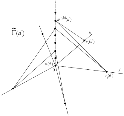
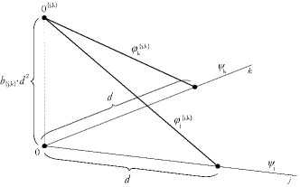
A possible way is to employ the bijection $b$ from the family of two-element subsets of $\{1,2,\ldots n\}$ to the set $\{1,2,\ldots\frac{n(n-1)}{2}\}$. The edge connecting the $j$-th and $k$-th halfline is formed by two segments connected in a V-shape. Its endpoints are at the $j$-th and $k$-th halfline, both at the distance $d$ from the centre. The tip of this $V$-graph is placed on the halfline starting from the centre of $\Gamma$ in the perpendicular direction to its plane – see Fig. 3 – at the distance $b_{jk}\cdot d^{2}$, so that the length of the connecting V-graph is $d\sqrt{1+(b_{jk}d)^{2}}$.

Refer to caption
Figure 3: The connecting edge between the $j$-th and $k$-th halfline

As before we denote by $\psi_{j}$ the wave function on the $j$-th halfline assuming that all the coordinates have zero in the centre of $\Gamma$. Furthermore, we denote by $\varphi^{\{j,k\}}_{j}$ and $\varphi^{\{j,k\}}_{k}$ the wave function on the line segment part of the connection between the $j$-th and $k$-th halfline which is attached by one of its endpoints to the $j$-th and $k$-th halfline, respectively; notice that the order of the upper indices is irrelevant. Such a connecting link is regarded as a star with two edges of the same length. For the sake of brevity we introduce also the set $N_{j}$ defined as

$$N_{j}=\{k\in\hat{n}:\>S_{jk}\neq 0\}\,;$$

its cardinality $\#N_{j}$ tells us how many nonzero elements are in the $j$-th row of the matrix $S$, in other words, how many V-shaped connecting edges sprout from the point $x_{j}=d$ on the $j$-th halfline.

Next we will write down the boundary conditions describing the involved $\delta$ couplings; for simplicity we will not indicate the dependence of the parameters $u,\,v_{j},\,w_{\{j,k\}}$ on the distance $d$. The $\delta$ coupling in the centre of $\Gamma$ means

$$\psi_{1}(0)=\psi_{2}(0)=\cdots=\psi_{n}(0)=:\psi(0)\,,\quad\sum^{n}_{j=1}\psi_{j}^{\prime}(0_{+})=u\psi(0)\,,$$ (60)

the $\delta$ interaction at the “tip” of the broken edge connecting the $j$-th and $k$-th halfline between the vertices added at the distance $d$ from the centre (of course, for $j,k\in\hat{n}$ such that $S_{jk}\neq 0$ only) is expressed through the conditions

$$\varphi^{\{j,k\}}_{j}(0)=\varphi^{\{j,k\}}_{k}(0)=:\varphi^{\{j,k\}}(0)\,,\;\;(\varphi^{\{j,k\}})_{j}^{\prime}(0_{+})+(\varphi^{\{j,k\}})_{k}^{\prime}(0_{+})=w_{\{j,k\}}\varphi^{\{j,k\}}(0)\,,$$ (61)

and finally, the $\delta$ coupling at the mentioned added vertices added requires

$$\begin{array}[]{c}\psi_{j}(d_{+})=\psi_{j}(d_{-})=\varphi^{\{j,k\}}_{j}\big{(}d\sqrt{1+(b_{jk}d)^{2}}\big{)}=:\psi_{j}(d)\,,\quad j\in\hat{n}\,,k\in N_{j}\\ \vspace{.5em}\psi_{j}^{\prime}(d_{+})-\psi_{j}^{\prime}(d_{-})-\sum_{k\in N_{j}}(\varphi^{\{j,k\}}_{j})^{\prime}\big{(}d\sqrt{1+(b_{jk}d)^{2}}_{-}\big{)}=v_{j}\psi_{j}(d)\,,\quad j\in\hat{n}\,.\end{array}$$ (62)

Further relations which will help us to find the parameter dependence on $d$ come from Taylor expansion,

$\displaystyle\psi_{j}(d)=\psi_{j}(0)+d\psi_{j}^{\prime}(0)+\mathcal{O})(d^{2})\,,\quad\psi_{j}^{\prime}(d_{-})=\psi_{j}^{\prime}(0_{+})+\mathcal{O}(d)\,,\quad j\in\hat{n}\,,$ (63)
$\displaystyle\begin{split}&\varphi^{\{j,k\}}_{j}\left(d\sqrt{1+(b_{jk}d)^{2}}\right)=\varphi^{\{j,k\}}(0)+d\sqrt{1+(b_{jk}d)^{2}}\,(\varphi^{\{j,k\}}_{j})^{\prime}(0_{+})+\mathcal{O}(d^{2})\,,\\ &(\varphi^{\{j,k\}}_{j})^{\prime}\left(d\sqrt{1+(b_{jk}d)^{2}}_{-}\right)=(\varphi^{\{j,k\}}_{j})^{\prime}(0_{+})+\mathcal{O}(d)\,,\quad j,k\in\hat{n}\,,\end{split}$ (64)

where we have used the fact that $\sqrt{1+(b_{jk}d)^{2}}=1+\mathcal{O}(d^{2})$. Now we employ the first of the relations (64) together with the continuity (62), which yields

$$d\sqrt{1+(b_{jk}d)^{2}}\>(\varphi^{\{j,k\}}_{j})^{\prime}(0_{+})=\psi_{j}(d)-\varphi^{\{j,k\}}(0)+\mathcal{O}(d^{2})\,.$$ (65)

The same relation holds with $j$ replaced by $k$, summing them together and using the second of the relations (61) we get

$$\left(2+d\sqrt{1+(b_{jk}d)^{2}}\>w_{\{j,k\}}\right)\varphi^{\{j,k\}}(0)=\psi_{j}(d)+\psi_{k}(d)+\mathcal{O}(d^{2})\,.$$

We express $\varphi^{\{j,k\}}(0)$ from here and substitute into (65) obtaining

$$d\sqrt{1+(b_{jk}d)^{2}}\>(\varphi^{\{j,k\}}_{j})^{\prime}(0_{+})=\psi_{j}(d)-\frac{\psi_{j}(d)+\psi_{k}(d)+\mathcal{O}(d^{2})}{2+d\sqrt{1+(b_{jk}d)^{2}}\cdot w_{\{j,k\}}}+\mathcal{O}(d^{2})\,.$$ (66)

The relations  (63) and (60) give

$$d\psi_{j}^{\prime}(0_{+})=\psi_{j}(d)-\psi(0)+\mathcal{O}(d^{2})\,,$$ (67)

and summing this over $j\in\hat{n}$ we arrive at the identity

$$d\sum^{n}_{j=1}\psi_{j}^{\prime}(0_{+})=\sum^{n}_{j=1}\psi_{j}(d)-n\psi(0)+\mathcal{O}(d^{2})\,.$$

The right-hand side of it can be rewritten using (60). This makes it possible to express $\psi(0)$; substituting it into (67) we get

$$d\psi_{j}^{\prime}(0_{+})=\psi_{j}(d)-\frac{\sum^{n}_{k=1}\psi_{k}(d)+\mathcal{O}(d^{2})}{n+du}+\mathcal{O}(d^{2})\,.$$ (68)

Next we use consecutively the second relations of (62), (63) and (64) to infer

$$\begin{split}\psi_{j}^{\prime}(d_{+})=&v_{j}\psi_{j}(d)+\sum_{k\in N_{j}}(\varphi^{\{j,k\}})_{k}^{\prime}\,\Big{(}d\sqrt{1+(b_{jk}d)^{2}}_{-}\Big{)}+\psi_{j}^{\prime}(d_{-})\\ =&v_{j}\psi_{j}(d)+\sum_{k\in N_{j}}(\varphi^{\{j,k\}})_{k}^{\prime}(0_{+})+\psi_{j}^{\prime}(0_{+})+\mathcal{O}(d)\,.\end{split}$$

Substituting into the last relation from (66) and (68) we get

$$\begin{split}\psi_{j}^{\prime}(d_{+})=&\left(v_{j}+\frac{1}{d}\left(\sum_{k\in N_{j}}\frac{1}{\sqrt{1+(b_{jk}d)^{2}}}+1\right)\right)\psi_{j}(d)\\ &-\frac{1}{d}\sum_{k\in N_{j}}\frac{1}{\sqrt{1+(b_{jk}d)^{2}}}\cdot\frac{\psi_{j}(d)+\psi_{k}(d)}{2+d\sqrt{1+(b_{jk}d)^{2}}\cdot w_{\{j,k\}}}\\ &-\frac{1}{d(n+du)}\left(\sum^{n}_{k=1}\psi_{k}(d)+\mathcal{O}(d^{2})\right)+\mathcal{O}(d)\,,\end{split}$$

where we have also employed the fact that $\mathcal{O}(d)\,[1+(b_{jk}d)^{2}]^{-1/2}=\mathcal{O}(d)$ holds as $d\to 0_{+}$ for all $j\neq k$, $j,k\in\hat{n}$.

Now we can finally ask about the parameter dependence on $d$. Since the last relation is supposed to yield in the limit $d\to 0_{+}$ the $j$-th row of the matrix condition (59), it would be sufficient to have the following requirements satisfied:

$$\lim_{d\to 0_{+}}\left(v_{j}+\frac{1}{d}\left(\sum_{k\in N_{j}}\frac{1}{\sqrt{1+(b_{jk}d)^{2}}}+1-\sum_{k\in N_{j}}\frac{1}{2+d\sqrt{1+(b_{jk}d)^{2}}w_{\{j,k\}}}\right)\right)=D_{j}$$ (69)

for all $j\in\hat{n}$,

$$\lim_{d\to 0_{+}}\frac{1}{d}\cdot\frac{1}{\sqrt{1+(b_{jk}d)^{2}}}\cdot\frac{-1}{2+d\sqrt{1+(b_{jk}d)^{2}}w_{\{j,k\}}}=S_{jk}$$ (70)

for all $j\neq k$, $j,k\in\hat{n}$, and finally

$$\frac{1}{d(n+du)}=\mathcal{O}(d)$$ (71)

as $d\to 0_{+}$. To fulfil (70) one can choose

$$w_{\{j,k\}}(d):=-\frac{1}{S_{jk}}\cdot\frac{1}{d^{2}}-\frac{2}{d}\,,$$ (72)

which makes sense because $S_{jk}\neq 0$ by assumption, since then the limit equals

$$\lim_{d\to 0_{+}}\frac{1}{1+\mathcal{O}(d^{2})}\cdot\frac{-1}{2d+(1+\mathcal{O}(d^{2}))\left(-\frac{1}{S_{jk}}-2d\right)}=S_{jk}\,.$$

With the choice (72) taken into account the condition (69) will be satisfied provided $v_{j}+\frac{1}{d}(\#N_{j}+1)-\sum_{k\in N_{j}}S_{jk}=D_{j}$, i.e.

$$v_{j}(d):=D_{j}-\frac{\#N_{j}+1}{d}-\sum_{k\in N_{j}}S_{jk}\,.$$ (73)

Finally, the last requirement will be satisfied, e.g., if the expression equals $d$ which is true if

$$u(d):=\frac{1}{d^{3}}-\frac{n}{d^{2}}\,.$$ (74)

Summarizing the argument we conclude that choosing the parameters in the described approximation according to (72)–(74) we get in the limit the generic boundary conditions (59). We conjecture that such an approximation would again converge in the norm-resolvent topology.

Acknowledgments

The research was supported by the Czech Academy of Sciences and Ministry of Education, Youth and Sports within the projects A100480501 and LC06002.

References

  • [1] K. Ruedenberg and C.W. Scherr, Free-electron network model for conjugated systems, I. Theory, J. Chem. Phys. 21 (1953), 1565–1581.
  • [2] N.I. Gerasimenko and B.S. Pavlov, Scattering problem on noncompact graphs, Teor. Mat. Fiz. 74 (1988), 345–359.
  • [3] P. Exner and P. Šeba, Free quantum motion on a branching graph, Rep. Math. Phys. 28 (1989), 7–26.
  • [4] S. Albeverio, F. Gesztesy, R. Høegh-Krohn and H. Holden, Solvable Models in Quantum Mechanics, 2nd edition (AMS Chelsea, 2005).
  • [5] P. Kuchment, Quantum graphs: I. Some basic structures, Waves in Random Media 14 (2004), S107–S128.
  • [6] G. Berkolaiko, R. Carlson, S. Fulling and P. Kuchment, eds., Quantum Graphs and Their Applications, Contemporary Math., vol. 415 (American Math. Society, Providence, R.I., 2006).
  • [7] M. Freidlin and A. Wentzell, Diffusion processes on graphs and the averaging principle, Ann. Prob. 21 (1993), 2215–2245.
  • [8] P. Kuchment and H. Zeng, Convergence of spectra of mesoscopic systems collapsing onto a graph, J. Math. Anal. Appl. 258 (2001), 671–700.
  • [9] J. Rubinstein and M. Schatzmann, Variational problems on multiply connected thin strips, I. Basic estimates and convergence of the Laplacian spectrum, Arch. Rat. Mech. Anal. 160 (2001), 271–308.
  • [10] T. Saito, Convergence of the Neumann Laplacian on shrinking domains, Analysis 21 (2001), 171–204.
  • [11] P. Exner and O. Post, Convergence of spectra of graph-like thin manifolds, J. Geom. Phys. 54 (2005), 77–115.
  • [12] O. Post, Spectral convergence of non-compact quasi-one-dimensional spaces, math-ph/0512081
  • [13] O. Post, Branched quantum wave guides with Dirichlet boundary conditions: the decoupling case, J. Phys. A: Math. Gen. 38 (2005), 4917–4931.
  • [14] S. Molchanov and B. Vainberg, Scattering solutions in a network of thin fibers: small diameter asymptotics, math-ph/0609021
  • [15] P. Exner: Weakly coupled states on branching graphs, Lett. Math. Phys. 38 (1996), 313–320.
  • [16] T. Cheon and T. Shigehara: Realizing discontinuous wave functions with renormalized short-range potentials, Phys. Lett. A243 (1998), 111–116.
  • [17] S. Albeverio and L. Nizhnik: Approximation of general zero-range potentials, Ukrainian Math. J. 52 (2000), 582–589.
  • [18] P. Exner, H. Neidhardt and V.A. Zagrebnov: Potential approximations to $\delta^{\prime}$: an inverse Klauder phenomenon with norm-resolvent convergence, Commun. Math. Phys. 224 (2001), 593–612.
  • [19] T. Cheon and P. Exner, An approximation to delta’ couplings on graphs, J. Phys. A: Math. Gen. 37 (2004), L329–335.
  • [20] P. Exner and O. Turek, Approximations of permutation-symmetric vertex couplings in quantum graphs, in Ref. [6], pp. 109–120.
  • [21] J.E. Avron, P. Exner, Y. Last, Periodic Schrödinger operators with large gaps and Wannier-Stark ladders, Phys. Rev. Lett. 72 (1994), 896–899.
  • [22] V. Kostrykin, R. Schrader, Kirchhoff’s rule for quantum wires, J. Phys. A: Math. Gen. 32 (1999), 595–630.
  • [23] M. Harmer, Hermitian symplectic geometry and extension theory, J. Phys. A: Math. Gen. 33 (2000), 9193–9203.
  • [24] V. Kostrykin, R. Schrader, Kirchhoff’s rule for quantum wires. II: The inverse problem with possible applications to quantum computers, Fortschr. Phys. 48 (2000), 703–716.
  • [25] P. Exner, Lattice Kronig-Penney models, Phys. Rev. Lett. 74 (1995), 3503–3506.
  • [26] P. Exner, Contact interactions on graph superlattices, J. Phys. A: Math. Gen. 29 (1996), 87–102.
  • [27] T. Shigehara, H. Mizoguchi, T. Mishima, T. Cheon T, Realization of a four parameter family of generalized one-dimensional contact interactions by three nearby delta potentials with renormalized strengths, IEICE Trans. Fund. Elec. Comm. Comp. Sci. E82-A (1999), 1708–1713.